Concentration inequalities for Paley-Wiener spaces

Abstract.

This article considers the question of how much of the mass of an element in a Paley-Wiener space can be concentracted on a given set. We seek bounds in terms of relative densities of the given set. We extend a result of Donoho and Logan from 1992 in one dimension and consider similar results in higher dimensions.

1. Introduction

Let $M$ be a convex body in $\mathbb{R}^{d}$, and let $\mathcal{B}_{p}(M)$, $1\leq p\leq\infty$, be the Paley-Wiener space of elements from $L^{p}(\mathbb{R}^{d})$ with distributional Fourier transform supported in $M$. The Fourier transform $\mathcal{F}f$ is given by

$$\mathcal{F}f(\varphi)=\int_{\mathbb{R}}\widehat{\varphi}(t)f(t)dt$$

for a Schwarz function $\varphi$. (We use $\widehat{\varphi}(t)=\int\varphi(x)e^{-2\pi ixt}dx$.) We write $\mathcal{B}_{p}(\tau)$ if $M$ is the ball with center at the origin and radius $\tau$.

Let $N$ and $W_{\delta}\subseteq\mathbb{R}^{d}$ be measurable and set $W_{\delta}(x)=x+W_{\delta}$. (In this article, $W_{\delta}$ is either a ball or a cube.) We consider the problem of finding a constant $C(M,\delta)>0$ such that

(1) $$\|G\chi_{N}\|_{1}\leq C(M,\delta)\sup_{x\in\mathbb{R}^{d}}|N\cap W_{\delta}(x)|\,\|G\|_{1}\text{ for all }G\in\mathcal{B}_{1}(M).$$

Here $|.|$ denotes Lebesgue measure and $\chi_{N}$ is the characteristic function of $N$. We emphasize that the constant is not allowed to depend on $N$.

This question was studied by Donoho and Logan [5] in dimension $d=1$ in connection with recovery of a bandlimited signal that is corrupted by noise. In their setting, an unknown noise $n\in L^{1}(\mathbb{R})$ is added to a known signal $F\in\mathcal{B}_{1}([-\tau,\tau])$, and they investigate sufficient conditions under which the best approximation $\widetilde{F}\in\mathcal{B}_{1}([-\tau,\tau])$ to $F+n$ satisfies $\widetilde{F}=F$, i.e., when $F$ can be perfectly recovered from knowledge of $F+n$ through best $L^{1}$-approximation.

Denoting now by $N$ the support of $n$, it is a remarkable fact that the concentration condition

(2) $$\frac{\|G\chi_{N}\|_{1}}{\|G\|_{1}}<\frac{1}{2}\textrm{ for all $G\in\mathcal{B}_{1}(M)$}$$

is sufficient to conclude that $F=\widetilde{F}$. The argument can be found in several places, e.g., Donoho and Stark [6, Section 6.2], who refer to it as Logan’s phenomenon. (Logan’s thesis [9] appears to contain the earliest record of this argument.) It was shown in [5, Theorem 7] that (1) holds for $W_{\delta}(x)=[x-\frac{\delta}{2},x+\frac{\delta}{2}]$ with

(3) $$C([-\tau,\tau],\delta)=\frac{\pi\tau}{\sin(\pi\tau\delta)},$$

and combining this with (2), it is evident that this gives $F=\widetilde{F}$ provided the relative density (or Nyquist density) of the support of the noise satisfies

$$\delta^{-1}\sup_{x\in\mathbb{R}}|N\cap[x,x+\delta]|<\frac{\sin(\pi\tau\delta)}{2\pi\tau\delta}.$$

We mention that conditions to recover an element of a closed subspace of an $L^{1}$ space that has been corrupted by a sparse $L^{1}$-noise have been investigated in many different settings, and concentration inequalities lead frequently to sufficient conditions. (This relies on the fact that if a set $N$ satisfies an analogue of (2) for all $G$ in a given closed subspace of an $L^{1}$-space, then the zero function is the closest element from the subspace to every $L^{1}$ function with support contained in $N$.) For interested readers we refer to Candès, Romberg, and Tao [3], Benyamini, Kroó, and Pinkus [2], Abreu and Speckbacher [1], and the references therein.

2. Results

There are two questions that this article seeks to address. First, it is clear that the shape of the bound in (3) requires $\delta\tau<1$. In contrast, it was shown for $p=2$ in [5, Theorem 4] that for any positive $\tau$ and $\delta$

$$\|G\chi_{N}\|_{2}^{2}\leq\left(\tau+\delta^{-1}\right)\sup_{x\in\mathbb{R}}\left|N\cap[x,x+\delta]\right|\,\|G\|_{2}^{2}$$

for all $G\in\mathcal{B}_{2}(\tau)$ (with constants adjusted due to the different normalization of the Fourier transform) which suggests that an inequality with constant $c(\tau+\delta^{-1})$ should also be true for $p=1$. Our first result confirms that this is the case.

Theorem 1.

Let $N$ be the support of $n\in L^{1}(\mathbb{R})$. Then for all $G\in\mathcal{B}_{1}(\tau)$

$$\|G\chi_{N}\|_{1}\leq C_{\tau,\delta}\sup_{x\in\mathbb{R}}\left|N\cap[x,x+\delta]\right|\,\|G\|_{1}.$$

where $C_{\tau,\delta}\leq\frac{80}{13}(\tau+\delta^{-1})$ for all positive $\tau$ and $\delta$. The bound may be improved to $C_{\tau,\delta}\leq\frac{5}{2}(\tau+\delta^{-1})$ for $\tau\delta\geq 2$. Moreover, $\lim_{\tau\delta\to\infty}C_{\tau,\delta}=2$.

As is usual with this method, the bounds only become effective when the density is a fraction of the reciprocal of the type $\tau$. If one is interested in bounds for $\|G\chi_{N}\|_{1}/\|G\|_{1}$ at larger densities, a version of the Logvinenko-Sereda theorem from O. Kovrijkine [8] gives non-trivial bounds whenever the density is smaller than $1$. The constants are not effective and don’t yield concrete bounds to decide when the quotient is $<1/2$.

Our second result deals with reconstruction in higher dimensions. We investigate the case when $M$ is a cube and $W_{\delta}(0)$ is a ball with center at the origin, and we indicate the obstructions that we encountered when taking $M$ to be a ball with center at the origin. We denote by $J_{\nu}$ the Bessel function of the first kind and by $j_{\nu}(k)$ its $k$th positive zero.

Theorem 2.

Let $d\in\mathbb{N}$ and let $N\subseteq\mathbb{R}^{d})$. If $\alpha\lambda<j_{d/2}(1)\,d^{-\frac{1}{2}},$ then for all $G\in\mathcal{B}_{1}([\lambda,\lambda]^{d})$

$$\|G\chi_{N}\|_{1} \leq\frac{(\sqrt{d}\lambda)^{d/2}}{\alpha^{d/2}J_{d/2}(2\pi\sqrt{d}\alpha\lambda)}\sup_{x\in\mathbb{R}^{d}}\left|N\cap B(x,\alpha)\right|\,\|G\|_{1}.$$

Analogously to dimension one, for a convex body $K$ we define the maximum Nyquist density of $N$ (relatively to $K$) by

$$\rho(N,K)=\frac{1}{|K|}\sup\limits_{u\in\mathbb{R}^{d}}|N\cap(u+K)|.$$

We compare the result of Theorem 2 to the case where the window $K$ is a hypercube of side length $\delta$, which is an extension of the $L_{1}$ reconstruction result by [5]. The zero $j_{p}(1)$ has an asymptotic expansion given in [4] by

$$j_{p}(1)\simeq\left(\frac{p}{2}+\frac{1}{4}\right)\pi.$$

Denote the ball of radius $r$ centered at origin by $B(0,r)$, and the volume of a ball with radius $\alpha$ in $d$-dimensions by $V_{d}(\alpha)$. It is given by $V_{d}(\alpha)=\frac{\pi^{d/2}}{\Gamma(d/2+1)}\alpha^{d}.$ When the window is a ball of radius $\alpha$, perfect reconstruction is possible if the maximum Nyquist density satisfies

$$\rho(N,B(0,\alpha))<\frac{\Gamma(d/2+1)J_{d/2}(2\pi\sqrt{d}\alpha\lambda)}{2(\pi\alpha\sqrt{d}\lambda)^{d/2}},$$

where $\alpha<\frac{j_{d/2}(1)}{2\pi\sqrt{d}\lambda}$. For $\lambda\delta<2\pi$, the corresponding density bound is

$$\rho(N,[-\delta/2,\delta/2]^{d})<\frac{1}{2}\left(\frac{\sin(\lambda\delta/2)}{\lambda\delta/2}\right)^{d}.$$

The support of the Fourier transform for both the problems is same, that is, $[-\lambda,\lambda]^{d}$. In the second case, we consider the ball just outside the cube such that the radius satisfies $\alpha=\frac{\delta\sqrt{d}}{2}$. Let $\delta=\frac{1}{2\pi^{2}}.$ For large $d$, the bound is asymptotically

$$\rho(T,B(0,\alpha),F) <\frac{\Gamma(d/2+1)J_{d/2}(d/2)}{2(d/4)^{d/2}}$$

$$\sim\frac{\sqrt{\pi d}\left(\frac{d}{2e}\right)^{d/2}}{2\left(\frac{d}{4}\right)^{d/2}}\frac{\Gamma(1/3)}{2^{1/3}\cdot 3^{1/6}\cdot\pi.d^{1/3}}$$

$$\sim d^{1/6}\left(\frac{2}{e}\right)^{d/2}$$

The Nyquist density for the cube window satisfies

$$\rho(T,[-\delta/2,\delta/2]^{d},F)<\frac{1}{2}\left(4\pi^{2}\sin(1/4\pi^{2})\right)^{d}.$$

The bound for the Nyquist density of the cube window remains larger than the bound for the Nyquist density of ball window for any $d$ in this case.

Third, we set the volume of the cube is equal to the volume of the ball. Then the radius $\alpha$ of the ball satisfies

$$\alpha=\delta\sqrt[d]{\frac{\Gamma(d/2+1)}{\pi^{d/2}}}.$$

Using Sterling’s approximation, we get

$$\alpha\simeq\delta\sqrt[d]{\left(\frac{d}{2\pi e}\right)^{d/2}(\pi d)^{1/2}}.$$

Let $\delta=\frac{\sqrt{2\pi e}}{4\pi^{2}}$. For large $d$, the Bessel function in the Nyquist density of the ball window satisfies

$$J_{d/2}(2\pi^{2}\sqrt{\alpha})=J_{d/2}(d\cdot\pi^{1/2d}\cdot d^{1/2d}/2)\rightarrow J_{d/2}(d/2),$$

since $\pi^{1/2d}\cdot d^{1/2d}\rightarrow 1$ for large $d$. The bound for the Nyquist density of the ball window is then

$$\rho(T,B(0,\alpha),F) <\frac{\Gamma(d/2+1)J_{d/2}(d/2)}{2\left(\pi^{2}\sqrt{d}\frac{\sqrt{2\pi e}}{4\pi^{2}\sqrt{\pi}}\sqrt[d]{\Gamma(d/2+1)}\right)}$$

$$\sim\frac{\Gamma(1/3).\pi^{1/4}}{2\cdot 2^{1/3}\cdot 3^{1/6}\cdot\pi}\left(\frac{4}{2e}\right)^{d/2}\frac{1}{d^{1/12}}$$

Tor the cube window, the sufficient bound for reconstruction is

$$\rho(T,[-\delta/2,\delta/2]^{d},F)<\frac{1}{2}\left(\frac{\sin(\sqrt{2\pi e}/8\pi)}{\sqrt{2\pi e}/8\pi}\right)^{d}.$$

In this case also, the Nyquist density for the cube window remains larger than the Nyquist density of ball window for any dimension $d$.

3. Proof of Theorem 1

We briefly review a general approach to prove inequalities of the above form introduced by Donoho and Logan in [5]. Construct a kernel $K(x,y)$ so that $f\mapsto Tf$ given by

$$Tf(y)=\int K(x,y)f(x)dx$$

defines a bounded invertible transformation when restricted to $\mathcal{B}_{1}(\tau)$. Then a change of integration order gives

$$\int_{N}|G(x)|dx \leq\int_{N}\int|K(x,y)|T^{-1}G(x)|dxdy$$

$$\leq\left(\sup_{x}\int_{N}K(x,y)dy\right)\|T^{-1}\|\|G\|_{1}.$$

If $K(x,y)=g(x-y)$ for some $g\in L^{\infty}$ with ${\rm supp}(g)\subseteq W_{\delta}(0)$, then the supremum may be further estimated by $\|g\|_{\infty}\sup_{x}|N\cap W_{\delta}(x)|$, where $T=T_{g}$ is now the convolution operator $T_{g}f=f*g$ restricted to $\mathcal{B}_{1}(\tau)$. For given $g$ the size of the constant depends then only on $\|g\|_{\infty}\|T_{g}^{-1}\|$, and (2) shows that we need

$$\sup_{x}|N\cap W_{\delta}(x)|<\frac{1}{2\|g\|_{\infty}\|T_{g}^{-1}\|}.$$

Thus, it is the task to construct $g$ as above where $\|g\|_{\infty}\|T_{g}^{-1}\|$ is as small as possible. The choice in [5] was $g=\chi_{[-\frac{\delta}{2},\frac{\delta}{2}]}$, which is optimal for $\delta\tau\leq\frac{1}{2}$, gives a non-optimal bound for $\frac{1}{2}<\delta\tau<1$, and fails to give a bound for $\delta\tau\geq 1$. This can be traced back to the fact that $\widehat{g}(\delta)=0$.

To create an auxiliary function $g$ with computable product $\|g\|_{\infty}\|T_{g}^{-1}\|$, Logan and Donoho observed that if $1/\widehat{g}$ is positive and convex up on an interval $I=[-a,a]$ with center at the origin, then the periodic extension of $1/\widehat{g}$ restricted to $I$ is the Fourier transform of a measure $\nu$ that acts as the inverse operator of convolution with $g$ on $\mathcal{B}_{1}(a)$ and has total variation $|\nu|=1/\widehat{g}(a)$. (In fact, $\nu$ is the minimal extrapolation of $1/\widehat{g}$ restricted to $I$ in the sense of Beurling.) Our choice of $g$ is based on this idea. We define for $\tau>0$ and real $x$ a function $g_{\tau}$, supported on $[-1,1]$, by

$$g_{\tau}(x)=-2(1-|x|)\frac{\cos 2\pi(\tau+1)x-\cos 2\pi\tau x}{4\pi^{2}x^{2}}\chi_{[-1,1]}(x).$$

The Fourier transform of $g_{\tau}$ has the useful property that the sum of its partials with respect to $t$ and $\tau$ has a simple integral representation.

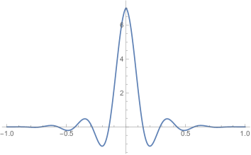
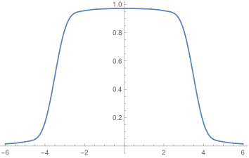
Figure 1. The transform pair $g_{4}(x)$ and $\widehat{g}_{4}(t)$

Proposition 1.

For any $t$ and $\tau$

$$\frac{\partial}{\partial t}\left(\widehat{g}_{\tau}(t)\right)+\frac{\partial}{\partial\tau}\left(\widehat{g}_{\tau}(t)\right)=\int_{2\pi(t+\tau)}^{2\pi(t+\tau+1)}\frac{\sin^{2}u}{u^{2}}du.$$

Proof.

For ease of notation we set $G(t,\tau)=\widehat{g}_{\tau}(t)$, and we denote first partials by $G_{t}$ and $G_{\tau}$. Writing

$$g_{\tau}(x)=2(1-|x|)\frac{\cos 2\pi(\tau+1)x-\cos 2\pi\tau x}{(-2\pi ix)^{2}}\chi_{[-1,1]}(x)$$

and using that $g_{\tau}(x)$ is even, we have

$$G_{t}(t,\tau) =\int_{-1}^{1}(-2\pi ix)g_{\tau}(x)e^{-2\pi ixt}dx$$

$$=\int_{-1}^{1}(-2\pi ix)g_{\tau}(x)(-i\sin(2\pi xt))dx$$

$$=\int_{-1}^{1}2(1-|x|)\frac{\cos(2\pi(\tau+1)x)-\cos(2\pi\tau x)}{2\pi x}\sin(2\pi xt)dx$$

$$=4\int_{0}^{1}(1-x)\frac{\cos(2\pi(\tau+1)x)-\cos(2\pi\tau x)}{2\pi x}\sin(2\pi xt)dx.$$

Similarly,

$$G_{\tau}(t,\tau) =\int_{-1}^{1}\frac{\partial}{\partial\tau}(g_{\tau}(x))e^{-2\pi ixt}dx$$

$$=4\int_{0}^{1}(1-x)\frac{\sin(2\pi(\tau+1)x)-\sin(2\pi\tau x)}{2\pi x}\cos(2\pi xt)dx.$$

The integrals have representations in terms of the sine-integral $\operatorname{Si}(u)=\int_{0}^{u}\sin(w)/wdw$. A direct calcuation gives

$$2\int_{0}^{1}\cos(2\pi ax)\frac{\sin(2\pi bx)}{x}dx =\operatorname{Si}(2\pi(a+b))-\operatorname{Si}(2\pi(a-b))$$

$$2\int_{0}^{1}\cos(2\pi ax)\sin(2\pi bx)dx =-\frac{b}{\pi(a-b)(a+b)}+\frac{\cos(2\pi(a-b))}{2\pi(a-b)}-\frac{\cos(2\pi(a+b))}{2\pi(a+b)}.$$

We obtain

$$G_{t}(t,\tau)+G_{\tau}(t,\tau) =\frac{2}{\pi^{2}}\left(\frac{\sin^{2}(\pi(t+\tau))}{(t+\tau)(t+\tau+1)}+\pi\operatorname{Si}(2\pi(t+\tau+1))-\pi\operatorname{Si}(2\pi(t+\tau)\right)$$

$$=\frac{2}{\pi}\int_{\pi(t+\tau)}^{\pi(t+\tau+1)}\left(-\frac{\partial}{\partial u}\frac{\sin^{2}u}{u}\right)du+\frac{2}{\pi}\int_{2\pi(t+\tau)}^{2\pi(t+\tau+1)}\frac{\sin w}{w}dw$$

$$=\frac{2}{\pi}\int_{\pi(t+\tau)}^{\pi(t+\tau+1)}\frac{\sin^{2}u}{u^{2}}du$$

after substituting $w=2u$ and combining the integrands. ∎

Corollary 1.

1. $\|g_{\tau}\|_{\infty}=g_{\tau}(0)=2\tau+1$.

2. The function $\tau\mapsto\widehat{g}_{\tau}(0)$ is positive, monotonically increasing, and has limit $1$ as $\tau\to\infty$. Moreover,

   $$\widehat{g}_{0}(0)>0.65,\qquad\widehat{g}_{1}(1)>0.8.$$

3. $t\mapsto\big{(}\widehat{g}_{\tau}(t)\big{)}^{-1}$ is positive and convex (up) on $[-\tau,\tau]$.

Proof.

Property (1) is obtained by direct calculation. For the proof of (2) it follows from symmetry of $t\mapsto\widehat{g}_{\tau}(t)$ that $\widehat{g}_{\tau}^{\prime}(0)=0$, and hence Proposition 1 gives $\partial/\partial\tau\widehat{g}_{\tau}(0)>0$. Direct calculations give the claimed bounds.

Regarding (3), we require an explicit representation of $\widehat{g}_{\tau}^{\prime\prime}(t)$. It follows from

$$g_{\tau}(x)=2(1-|x|)\frac{\cos 2\pi(\tau+1)x-\cos 2\pi\tau x}{(-2\pi ix)^{2}}\chi_{[-1,1]}(x)$$

that

(4) $$\begin{split}\widehat{g}_{\tau}^{\prime\prime}(t)&=\int_{-1}^{1}(-2\pi ix)^{2}g_{\tau}(x)e^{-2\pi ixt}dx\\ &=-\left(\frac{\sin\pi(t-\tau)}{\pi(t-\tau)}\right)^{2}-\left(\frac{\sin\pi(t+\tau)}{\pi(t+\tau)}\right)^{2}\\ &\qquad\qquad\qquad\qquad+\left(\frac{\sin\pi(t-\tau-1)}{\pi(t-\tau-1)}\right)^{2}+\left(\frac{\sin\pi(t+\tau+1)}{\pi(t+\tau+1)}\right)^{2}\\ &=\frac{\sin^{2}(\pi(t-\tau))(2(t-\tau)-1)}{(t-\tau)^{2}(t-\tau-1)^{2}}-\frac{\sin^{2}(\pi(t+\tau))(2(t+\tau)+1)}{(t+\tau)^{2}(t+\tau+1)^{2}}.\end{split}$$

Since the first term is negative for $t-\tau<1/2$ and the second term is positive for $t+\tau>-1/2$, it follows that

$$\widehat{g}_{\tau}^{\prime\prime}(t)<0\text{ for }-\tau-\tfrac{1}{2}<t<\tau+\frac{1}{2}.$$

Multivariate chain rule and Proposition 1 show that

$$\frac{\partial}{\partial\tau}\left(\widehat{g}_{\tau}(\tau)\right)>0,$$

and since $\widehat{g}_{0}(0)>0$, it follows that $\widehat{g}_{\tau}(\tau)>0$ for all $\tau$. Since $\widehat{g}_{\tau}$ is concave down on $[-\tau,\tau]$, it follows that $\widehat{g}_{\tau}(t)>0$ for $t\in[-\tau,\tau]$. It follows that the second derivative of $t\mapsto(\widehat{g}_{\tau}(t))^{-1}$ is positive for $|t|\leq\tau$. ∎

Proof of Theorem 1.

Setting $g_{\tau,\delta}(x)=g_{\tau\delta/2}(2x/\delta)$, we observe that $g_{\tau,\delta}$ is supported on $[-\delta/2,\delta/2]$, and

$$\widehat{g}_{\tau,\delta}(t)=\frac{\delta}{2}\widehat{g}_{\tau\delta/2}(\delta t/2).$$

It follows that $t\mapsto(\widehat{g}_{\tau,\delta}(t))^{-1}$ is positive and convex up for $|t|\leq\tau$. Let $a_{n}=a_{n}(\tau,\delta)$ be the Fourier coefficients satisfying

$$\frac{1}{\widehat{g}_{\tau,\delta}(t)}=\sum_{n\in\mathbb{Z}}a_{n}e^{\pi i\frac{t}{\tau}n}$$

for $|t|\leq\tau$. Positivity and convexity imply that $|a_{n}|=(-1)^{n}a_{n}$. Define a measure $\nu=\nu_{\tau,\delta}$ on $\mathbb{R}$ for any Borel set $A$ by

$$\nu(A)=\sum_{n\in\mathbb{Z}}a_{n}\delta_{n/(2\tau)}(A)$$

where $\delta_{b}$ is the Dirac measure at $b\in\mathbb{R}$. We observe that $\widehat{\nu}(t)=1/\widehat{g}_{\tau,\delta}(t)$ for $|t|\leq\tau$, and the total variation satisfies

$$|\nu|(\mathbb{R})=\sum_{n\in\mathbb{Z}}|a_{n}|=\sum_{n\in\mathbb{Z}}a_{n}(-1)^{n}=\frac{1}{\widehat{g}_{\tau\delta/2}(\tau\delta/2)}.$$

It follows that convolution with $\nu$ is the inverse operator of convolution with $g_{\tau,\delta}$ when restricted to $PW_{\tau}^{1}$. Moreover, for $g_{\tau,\delta}$ the choice of $\nu$ is optimal, since the value of the Fourier transform of $\nu$ is always a lower bound for the total variation.

It follows that

$$\|T_{g_{\tau,\delta}}^{-1}\|=\frac{1}{\widehat{g}_{\tau\delta/2}(\tau\delta/2)}.$$

We observe the identities

$$\frac{\|g_{\tau,\delta}\|_{\infty}}{\widehat{g}_{\tau,\delta}(\tau)}=\frac{2}{\delta}\frac{\|g_{\tau\delta/2}\|_{\infty}}{\widehat{g}_{\tau\delta/2}(\tau\delta/2)}=\frac{2\tau+2\delta^{-1}}{\widehat{g}_{\tau\delta/2}(\tau\delta/2)}.$$

For $\tau>0$ and $\delta>0$ we use the inequality $\widehat{g}_{\tau\delta/2}(\tau\delta/2)\geq\widehat{g}_{0}(0)>0.65$. For $\tau\delta\geq 2$, we may use the lower bound $\widehat{g}_{1}(1)>0.8$ instead. ∎

4. Proof of Theorem 2

As in the first section, the main task lies in computing a minimal extrapolation of $1/\widehat{g}$ restricted support of the Fourier transform for a suitably chosen function $g$. For $x\in\mathbb{R}^{d}$ we consider

$$g_{\alpha}(x)=\chi_{B(0,\alpha)}(x)$$

whose Fourier transform for $t\in\mathbb{R}^{d}$ is

$$\widehat{g}_{\alpha}(t)=\frac{\alpha^{d/2}J_{d/2}(2\pi\alpha|t|)}{|t|^{d/2}}.$$

To construct a minimal extrapolation of $1/\widehat{g}_{\alpha}$ restricted to $[-\tau,\tau]^{d}$, we need facts from the theory of Laguerre-Pólya entire functions. We follow [7]. An entire function $E$ belongs to the Laguerre-Pólya class $\mathcal{E}$ if and only if it has the form

$$E(s)=e^{cs^{2}+bs}\prod\limits_{k=1}^{\infty}\left(1-\frac{s}{a_{k}}\right)e^{\frac{s}{a_{k}}},$$

where $c\geq 0$, $b$, $a_{k}(k=1,2,\cdots)$ are real, and

$$\sum_{k=1}^{\infty}\frac{1}{a_{k}^{2}}<\infty.$$

Lemma 1.

There exists a non-negative, integrable function $G$ such that for $x\in(-j_{p}(1),j_{p}(1))$

$$\frac{x^{p}}{J_{p}(x)}=\int\limits_{-\infty}^{0}e^{-x^{2}t}G(t)dt.$$

Proof.

The Bessel function $J_{p}(x)$ has an infinite product representation [4, Section 10.21(iii)]. Dividing each side by $x^{p}$ gives us

$$\frac{J_{p}(x)}{x^{p}} =\frac{1}{2^{p}\Gamma(p+1)}\prod\limits_{k=1}^{\infty}\left(1-\frac{x^{2}}{j_{p,k}^{2}}\right)$$

$$=\frac{1}{2^{p}\Gamma(p+1)}\prod\limits_{k=1}^{\infty}\left(1-\frac{x}{j_{p,k}}\right)e^{x/j_{p,k}}\prod\limits_{k=1}^{\infty}\left(1+\frac{x}{j_{p,k}}\right)e^{-x/j_{p,k}}$$

Substituting $x=\sqrt{y}$ in the infinite product representation of $\frac{J_{p}(x)}{x^{p}}$ gives us

$$\frac{J_{p}(\sqrt{y})}{y^{p/2}}=\frac{1}{2^{p}\Gamma(p+1)}\prod\limits_{k=1}^{\infty}\left(1-\frac{y}{j_{p,k}^{2}}\right)$$

which is an entire function and belongs to class $\mathcal{E}$. Let $E(x)=\frac{J_{p}(x)}{x^{p}}$. Then by [7, Theorem 6.1] the function $1/E(\sqrt{y})$ has a Laplace transform representation given by

$$\frac{1}{E(\sqrt{y})}=\int\limits_{\mathbb{R}}e^{-yt}G(t)dt,$$

where $G(t)\in C^{\infty}$ is a nonnegative, integrable function and the integral converges in the largest vertical strip which contains the origin and is free of zeroes of $E(\sqrt{y})$, which is $-\infty<y<j_{p,1}^{2}$. Next, we want to determine the values of $t$ for which $G(t)>0$. This result is obtained using Corollary 3.1 (Chapter 5 in [7]). Note that $E(\sqrt{y})$ can be expressed as

$$E(\sqrt{y}) =\frac{1}{2^{p}\Gamma(p+1)}\prod\limits_{k=1}^{\infty}\left(1-\frac{y}{j_{p,k}^{2}}\right)$$

$$=\frac{1}{2^{p}\Gamma(p+1)}\frac{1}{e^{-\sum\limits_{k=1}^{\infty}(y/j_{p,k})}}\prod\limits_{k=1}^{\infty}\left(1-\frac{y}{j_{p,k}^{2}}\right)e^{(y/j_{p,k})}$$

The function $E(\sqrt{y})$ has no negative zeroes. Therefore, in the setting of Corollary 3.1, $\alpha_{1}=-\infty$ and $b=-\sum\limits_{k=1}^{\infty}\frac{1}{j_{p,k}}$. Therefore $G(t)>0$ if $t\in(-\infty,0))$ and $G(t)=0$ otherwise, giving us for $y\in(0,j_{p,1}^{2})$,

$$\frac{1}{E(\sqrt{y})}=\int\limits_{-\infty}^{0}e^{-yt}G(t)dt.$$

Substituting $y=x^{2}$ gives the claim. ∎

Let $\lambda>0$ and $\alpha>0$ with $2\pi\sqrt{d}\alpha\lambda<j_{d/2}(1)$. We construct a (signed) measure $\nu$ that is an inverse transform on $\mathcal{B}_{1}([-\lambda,\lambda]^{d})$ of convolution with $g_{\alpha}$ satisfying

$$\|f*\nu\|_{1}\leq\frac{(\sqrt{d}\lambda)^{d/2}}{\alpha^{d/2}J_{d/2}(2\pi\sqrt{d}\lambda\alpha)}\|f\|_{1},$$

and we show that the constant is best possible among all inverse transformations of convolution with $g_{\alpha}$ on $\mathcal{B}_{1}([-\lambda,\lambda]^{d})$. We expand $1/\widehat{g}_{\alpha}$ restricted to $[-\lambda,\lambda]^{d}$ into its Fourier series

$$\frac{1}{\widehat{g}_{\alpha}(t)}=\sum_{n\in\mathbb{Z}^{d}}H_{\alpha}(n)e^{2\pi int}$$

where

$$H_{\alpha}(n)=\left(\frac{1}{2\lambda}\right)^{d}\int_{[-\lambda,\lambda]^{d}}\frac{|x|^{d/2}}{\alpha^{d/2}J_{d/2}(2\pi\alpha|x|)}e^{-i\frac{\pi}{\lambda}nx}dx.$$

Lemma 2.

The coefficients satisfy

$$H(n_{1},...,n_{d})=(-1)^{n_{1}+...+n_{d}}|H(n_{1},...,n_{d})|$$

Proof.

The restrictions on $\alpha\lambda$ imply that the following integrals converge absolutely. Inserting the Schoenberg representation (LABEL:) gives with $n=(n_{1},...,n_{d})$

$$H_{\alpha}(n)=\left(\frac{1}{2\sqrt{2\pi}\alpha\lambda}\right)^{d}\int_{-\infty}^{0}G(t)\left(\prod_{j=1}^{d}\int_{[-\lambda,\lambda]}e^{-x_{j}^{2}t}e^{-i\frac{\pi}{\lambda}n_{j}x_{j}}dx_{j}\right)dt$$

Since $t<0$, the function $x_{j}\mapsto e^{-tx_{j}^{2}}$ is positive, symmetric, and convex up. Hence $e^{-i\frac{\pi}{\lambda}n_{j}x_{j}}$ may be replaced by $\cos(\frac{\pi}{\lambda}n_{j}x_{j})$. A short argument involving two integration by parts may be used to show that

$$(-1)^{n_{j}}\int_{[-\lambda,\lambda]}e^{-x_{j}^{2}t}\cos(\tfrac{\pi}{\lambda}n_{j}x_{j})dx_{j}\geq 0,$$

which implies the claim of the lemma. ∎

We define a measure $\nu_{\alpha}$ on $\mathbb{R}^{d}$ by

$$\nu_{\alpha}=\sum_{n\in\mathbb{Z}^{d}}H_{\alpha}(n)\delta_{\frac{n}{2\lambda}}$$

where $\delta_{x}$ is the point measure at $x$ with $\delta_{x}(\mathbb{R}^{d})=1$.

Lemma 3.

Let $\lambda$ and $\alpha$ be positive with $2\pi\sqrt{d}\lambda\alpha<j_{d/2}(1)$. Convolution with $\nu_{\alpha}$ is the inverse operator of convolution with $g_{\alpha}$ on $\mathcal{B}_{1}([-\lambda,\lambda]^{d}$ with

$$\|f*\nu_{\alpha}\|_{1}\leq\frac{(\sqrt{d}\lambda)^{d/2}}{\alpha^{d/2}J_{d/2}(2\pi\sqrt{d}\alpha\lambda)}\|f\|_{1}$$

for all $f\in\mathcal{B}_{1}([-\lambda,\lambda]^{d})$.

Proof.

By construction of $\nu_{\alpha}$ we have

$$\widehat{g}_{\alpha}(t)\widehat{\nu}_{\alpha}(t)=1$$

for all $t\in[-\lambda,\lambda]^{d}$, and we observe that the total variation measure $|\nu_{\alpha}|$ satisfies

$$|\nu_{\alpha}|(\mathbb{R}^{d})=\sum_{n\in\mathbb{Z}^{d}}|H_{\alpha}(n)|=\sum_{n\in\mathbb{Z}^{d}}H_{\alpha}(n)(-1)^{n_{1}+...+n_{d}}=\frac{1}{\widehat{g}_{\alpha}(\lambda,...,\lambda)},$$

and Minkowski’s inequality $\|f*\nu_{\alpha}\|_{1}\leq|\nu_{\alpha}|\,\|f\|_{1}$ shows that convolution with $\nu_{\alpha}$ defines a bounded operator on $\mathcal{B}_{1}([-\lambda,\lambda]^{d})$ that inverts convolution with $g_{\alpha}$. ∎

Lemma 3 gives a bound for the operator norm of the inverse of convolution with $g_{\alpha}$, and the calculation at the beginning of the proof of Theorem 1 may be used to complete the proof of Theorem 2.

References

[1]
L. D. Abreu and M. Speckbacher, Donoho-Logan large sieve principles for
modulation and polyanalytic Fock spaces, Bull. Sci. Math. 171
(2021), Paper No. 103032, 25. MR 4295117
[2]
Y. Benyamini, A. Kroó, and A. Pinkus, -approximation and
finding solutions with small support, Constr. Approx. 36 (2012),
no. 3, 399–431. MR 2996438
[3]
E. J. Candès, J. Romberg, and T. Tao, Robust uncertainty principles:
exact signal reconstruction from highly incomplete frequency information,
IEEE Trans. Inform. Theory 52 (2006), no. 2, 489–509. MR 2236170
[4]NIST Digital Library of Mathematical Functions,
http://dlmf.nist.gov/, Release 1.1.6 of 2022-06-30, F. W. J. Olver, A. B.
Olde Daalhuis, D. W. Lozier, B. I. Schneider, R. F. Boisvert, C. W. Clark,
B. R. Miller, B. V. Saunders, H. S. Cohl, and M. A. McClain, eds.
[5]
D. L. Donoho and B. F. Logan, Signal recovery and the large sieve, SIAM
J. Appl. Math. 52 (1992), no. 2, 577–591. MR 1154788
[6]
D. L. Donoho and P. B. Stark, Uncertainty principles and signal
recovery, SIAM J. Appl. Math. 49 (1989), no. 3, 906–931.
MR 997928
[7]
I. I. Hirschman and D. V. Widder, The convolution transform, Princeton
University Press, Princeton, N. J., 1955. MR 0073746
[8]
Oleg Kovrijkine, Some results related to the Logvinenko-Sereda
theorem, Proc. Amer. Math. Soc. 129 (2001), no. 10, 3037–3047.
MR 1840110
[9]
B. F. Logan, Properties of high-pass signals, Ph.D. thesis, Columbia
University, 1965.