Linear Regression with Centrality Measures

Abstract

This paper studies the properties of linear regression on centrality measures when network data is sparse – that is, when there are many more agents than links per agent – and when they are measured with error. We make three contributions in this setting: (1) We show that OLS estimators can become inconsistent under sparsity and characterize the threshold at which this occurs, with and without measurement error. This threshold depends on the centrality measure used. Specifically, regression on eigenvector is less robust to sparsity than on degree and diffusion. (2) We develop distributional theory for OLS estimators under measurement error and sparsity, finding that OLS estimators are subject to asymptotic bias even when they are consistent. Moreover, bias can be large relative to their variances, so that bias correction is necessary for inference. (3) We propose novel bias correction and inference methods for OLS with sparse noisy networks. Simulation evidence suggests that our theory and methods perform well, particularly in settings where the usual OLS estimators and heteroskedasticity-consistent/robust $t$-tests are deficient. Finally, we demonstrate the utility of our results in an application inspired by De Weerdt and Dercon (2006), in which we consider consumption smoothing and social insurance in Nyakatoke, Tanzania.

Keywords: networks, diffusion centrality, eigenvector centrality.

JEL Classification Codes: C18, C21, C81.

1 Introduction

A large and rapidly growing body of work documents the influence of networks in a wide range of economic outcomes: peer effects drive academic achievement, production networks shape shock propagation in the macroeconomy, social networks affect information- and risk-sharing with important implications for development (see Sacerdote 2011, Carvalho and Tahbaz-Salehi 2019 and Breza et al. 2019 for recent reviews). Many other examples abound.

One particular strand of research has fruitfully explored the relationship between an agent’s network position and their economic outcomes. For example, Hochberg et al. (2007) considers the network of venture capital firms and finds that better-networked firms successfully exit a greater proportion of their investments. Meanwhile, Cruz et al. (2017) examines the social networks in the Philippines and shows that more central families are disproportionately represented in political offices. Similarly, Banerjee et al. (2013) studies the problem of diffusing microfinance in India and establishes that seeding information to more central agents led to greater participation in the program.

In these papers, researchers often estimate linear models by ordinary least squares (OLS), using centrality measures as explanatory variables. Centrality measures are node-level statistics that capture notions of importance in a network. Since nodes can be important for many reasons, a variety of centrality measures exist, each capturing a particular aspect of network position. For example, the degree centrality of an agent reflects the number or intensity of their direct links, while eigenvector centrality is designed so that influence of agents is proportional to that of their connections. The correlation between an outcome variable and a particular centrality measure may be revealing about the types of interactions that drive a given economic phenomenon: an outcome that is well-predicted solely by degree is likely to be determined in an extremely local manner, whereas one that is more strongly associated with eigenvector centrality may involve non-linear interactions between agents that are further apart. As such, when researchers estimate these correlations and test their statistical significance, they frequently do so with the goal of drawing conclusions about the economic significance of various centrality measures and the implied mechanisms for outcome determination. Such an exercise is credible only if the OLS estimator is close to the estimand, and if the chosen test statistic (typically the heteroskedasticity-consistent/robust $t$-statistics) is well described by its asymptotic distribution (standard normal for $t$-statistics) in finite sample.

However, network data have two features that may threaten the statistical validity of OLS. Firstly, networks may be sparse, with many more agents than links per agent. This could happen because interactions are observed with low frequency, or because the interactions in question are rare. Chandrasekhar (2016) argues that many economic networks are sparse, providing evidence from commonly used social network data (e.g. AddHealth; Karnataka Villages (Banerjee et al. 2013); Harvard social network (Leider et al. 2009)). Sparsity poses a challenge to estimation and inference: if networks are largely empty, there might not be enough variation in centrality measures to identify the parameters of interest. Despite its importance, sparsity has received relatively little attention in the network econometrics literature.

Secondly, the observed network may differ from the true network of interest. Centrality measures are often calculated on data which are obtained by survey or constructed using some proxy for interaction between agents, though subsequent analysis would frequently treat the true network as known. Ignoring measurement error may thus lead to estimates that perform poorly. A growing literature works with networks that are assumed to be measured with error. However, they generally do not consider sparse settings. This is important since sparsity and measurement error are mutually reinforcing: sparser networks contain weaker signals, which are in turn more difficult to pick out from noisy measurements. The upshot is that OLS estimators computed on sparse, noisy networks may have particularly poor properties. Asymptotic theory that ignore these features will provide similarly poor approximations to their finite sample behavior. Consequently, estimation and inference procedures based on these theories may lead to invalid conclusions about the economic significance of centrality measures.

This paper studies the statistical properties of OLS on centrality measures in an asymptotic framework which features both measurement error and sparsity. Our analysis is centered on degree, diffusion and eigenvector centralities, which are among the most popular measures. Our contribution is threefold: (1) We characterize the amount of sparsity at which OLS estimators become inconsistent with and without measurement error, finding that this threshold varies depending on the centrality measure used. Specifically, regression on eigenvector centrality is less robust to sparsity than that on degree and diffusion. This suggests that researchers should be cautious about comparing regressions on different centrality measures, since they may differ in statistical properties in addition to economic significance. (2) We develop distributional theory for OLS estimators under measurement error and sparsity. We restrict ourselves to sparsity ranges under which OLS is consistent, but we find that asymptotic bias can be large even in this case. Furthermore, the bias may be of larger order than variance, in which case bias correction would be necessary for obtaining non-degenerate asymptotic distributions. Additionally, we find that under sparsity, the estimator converges at a slower rate than is reflected by the usual heteroskedasticity-consistent(hc)/robust standard errors, requiring a different estimator. (3) In view of the distributional theory, we propose novel bias-corrected estimators and inference methods for OLS with sparse, noisy networks. We also clarify the settings under which hc/robust $t$-statistics are appropriate for testing.

Our theoretical results are derived in an asymptotic framework where networks are modeled as realizations of sparse random graphs. As $n\to\infty$, the expected number of links per agent grows much more slowly than $n$. Because our statistical model captures important features of real world data, we expect our methods to be reliable for estimation and inference with sparse, noisy networks. We provide simulation evidence supporting this view. The utility of our results is also evident from an application inspired by De Weerdt and Dercon (2006), where we conduct a stylized study of consumption smoothing and social insurance in Nyakatoke, Tanzania.

Our choice of asymptotic framework poses technical challenges. Firstly, the eigenvectors and eigenvalues of sparse random graphs are difficult to characterize. We draw on recent advances in random matrix theory (Alt et al. 2021a; b; Benaych-Georges et al. 2019; 2020) to overcome this challenge. Secondly, spectral norms of random matrices concentrate slowly in sparse regimes. Instead, we develop bounds for moments of noisy adjacency matrices by relating them to counts of particular graphs, in the spirit of Wigner (1957) (see Chapter 2 of Tao 2012 more generally). Finally, in order for bias correction to improve mean-squared error, the bias needs to be estimated at a sufficiently fast rate. Because variance is of lower order than bias, a naive plug-in approach does not work for estimating higher order bias terms, although it is sufficient for the first order term. We leverage this fact to recursively construct good estimators for higher order terms.

Related Literature

Our work is most closely related to papers that study linear regression with centrality statistics. To our best knowledge, we are the first to study linear regression with diffusion centrality, though there exist prior work on eigenvector centrality. Le and Li (2020) studies linear regression on multiple eigenvectors of a network assuming the same type of measurement error as this paper. They focus on denser settings than we do and provide inference method only for the null hypothesis that the slope coefficient is $0$. We are concerned only with eigenvector centrality, which is the leading eigenvector, but our results cover the sparse case as well as tests of non-zero null hypotheses (more details in Remark 5). Our paper is also related to Cai et al. (2021), which proposes penalized regressions on the leading left and right singular vectors of a network. They consider networks that are as sparse as the ones we study, but their networks are observed with an additive, normally distributed error (more details in Remark 4). Outside of the linear regression setting, Cheng et al. (2021) considers inference on deterministic linear functionals of eigenvectors. They study symmetric matrices with asymmetric noise, proposing novel estimators that leverage asymmetry to improve performance when eigengaps are small. We focus on symmetric matrices with symmetric noise and study the plug-in estimator in which eigenvector is estimated using the noisy adjacency matrix in place of the true matrix.

Our paper also relates to a growing literature that considers sampling and measurement error in networks. Chandrasekhar and Lewis (2016) examines settings in which researchers have access to a panel of networks, but which are constructed using only a partial sample of nodes or edges. Thirkettle (2019) studies a similar missing data problem, but in a cross-sectional setting with only one network. It is concerned with forming bounds on centrality statistics and does not consider subsequent linear regression. Griffith (2022) considers the censoring in network data, which arises when agents are only allowed to list a fixed number of relationships during the sampling process. The above papers study missing data problems under the assumption that the observed network is without error. We assume that the entirety of one network is observed but with error. Lewbel et al. (2021) studies measurement error in peer effects regression, finding that 2SLS with friends-of-friends instruments is valid as long as measurement error is small. They do not discuss centrality regressions.

This paper is also connected to the nascent literature on the statistical properties of sparse networks. A strand of this literature is concerned with network formation models that can give rise to sparsity in the observed data. Dong et al. (2020) and Motalebi et al. (2021) consider modifications to the stochastic block model. A more general model takes the form of inhomogeneous Erdos-Renyi graph, which are generated by a graphon with a sparsity parameter that tends to zero in the limit (see for instacne Bollobás et al. 2007 and Bickel and Chen 2009). Our paper takes this approach. Yet another model for sparse graphs is based on graphex processes, which generalizes graphons by generating vertices through Poisson point processes (see Borgs et al. 2018, Veitch and Roy 2019 and references therein). Our choice of inhomogeneous Erdos-Renyi graphs is motivated by their prevalence in econometrics (Section 3 of De Paula 2017 and Section 6 of Graham 2020a provide many examples), as well as tractability considerations. To our best knowledge, few papers have tackled the challenges that sparse networks pose for regression. Two notable exceptions study network formation models, which take the form of edge-level logistic regressions (Jochmans 2018; Graham 2020b). A separate literature considers estimation of peer effects regressions involving sparse networks using panel data (Manresa 2016; Rose 2016; De Paula et al. 2020). Here, sparsity is an assumption used to justify regularization methods. We consider a node-level regression in a cross-sectional setting with one large network.

More generally, we contribute to the literature on measurement error models, in which economic outcomes are driven by unobserved latent variables, although proxies or noisy measurements of these variables exist. For recent reviews, see Hu (2017) and Schennach (2020). Classical measurement error is an additive noise that is (conditionally) independent of the unobserved regressor and has a long history (e.g. Adcock 1878). When the underlying network is noisily observed, centrality statistics face errors which are non-linear and non-separable. General non-classical measurement error problems have been studied in cross-sectional (e.g. Matzkin 2003; Chesher 2003; Evdokimov and Zeleneev 2022) and panel data settings (e.g. Griliches and Hausman 1986; Evdokimov 2010; Evdokimov and Zeleneev 2020). These papers typically assume that observations can be grouped into units across which the latent variable and measurement error are independent. This excludes our setting, since centrality statistics of any given agent depends on the entire network.

The rest of this paper is organized as follows. Section 2 describes the set-up of our paper. Section 3 presents the theoretical results. Simulation results are contained in Section 4. In Section 5, we apply our results to the social insurance network in Nyakatoke, Tanzania. Section 6 concludes the paper with our recommendations for empirical work. All proofs are contained in Appendix A.

2 Set-Up and Notation

In this section, we introduce notation before describing our econometric model and the asymptotic framework.

We use the following notation. When $X$ is a vector or matrix, $X_{i}$ and $X_{ij}$ refer the $i^{\text{th}}$ and $(i,j)^{\text{th}}$ component of $X$ respectively. Similarly, if $X_{i}$ or $X_{ij}$ are defined, we use $X$ to denote the full vector or matrix respectively. $X^{\prime}$ is the transpose of $X$. When $X$ is a square matrix, $\lambda_{j}(X)$ denotes the $j^{\text{th}}$ eigenvalue of $X$ while $v_{j}(X)$ denotes the corresponding eigenvector. When $f\in L^{2}([0,1]^{2})$ is a symmetric real function, $\lambda_{j}(f)$ denotes the $j^{\text{th}}$ eigenvalue of the corresponding Hillbert-Schmidt integral operator, $T(g)=\int f(x,y)g(y)dy$, while $\phi_{j}$ is the corresponding eigenfunction. For deterministic, monotone sequences $x_{n}$ and $y_{n}$, we write $x_{n}\succ z_{n}$ if $x_{n}/z_{n}\to\infty$ and $x_{n}\prec z_{n}$ if $x_{n}/z_{n}\to 0$. $x_{n}\approx z_{n}$ indicates that $x_{n}/z_{n}\to k$, where $0<k<\infty$. We write $x_{n}\succcurlyeq z_{n}$ to mean $\neg(x_{n}\prec z_{n})$ and similarly for $x_{n}\preccurlyeq z_{n}$. Let $\iota_{n}$ be the $n\times 1$ vector of $1$’s. For two $m\times n$ matrices $X$ and $Z$, let $X\circ Z$ denote their entrywise (Hadamard) product. Finally, $[n]$ denotes the set of integers from $1$ to $n$.

2.1 Econometric Framework

For simplicity, suppose that there are no covariates besides centrality. Suppose also that the data-generating process yields $\{(Y_{i},U_{i})\}_{i=1}^{n}$ which are independent and identically distributed. $Y_{i}$ is the observed outcome of interest. $U_{i}$ is an unobserved latent type that will be used to construct the network. In lieu of $U_{i}$, we observe either the true adjacency matrix $A$, or a noisy version, $\hat{A}$. $A$ is an $n\times n$ matrix whose $(i,j)^{\text{th}}$, $A_{ij}$, records the link intensities between agents $i$ and $j$. $\hat{A}$ is some estimate of $A$.

Consider the regression:

$$Y_{i}=\beta^{(d)}C^{(d)}_{i}+\varepsilon_{i}$$

where $C^{(d)}_{i}$ is a network centrality measure of type $d$. We do not observe $C^{(d)}_{i}$, it can be exactly computed using $A$, or estimated using $\hat{A}$. The parameter of interest is $\beta^{(d)}$. After defining the data-generating process for the latent and observed networks, Assumption 3 will provide conditions allowing us interpret $\beta^{(d)}$ as the slope coefficient in the linear conditional expectation function of $Y_{i}$ on $C_{i}^{(d)}$.

In the following, we describe (i) the data-generating process for $A$ and $\hat{A}$ via the $U_{i}$’s and (ii) the use of $A$ and $\hat{A}$ in computing/estimating centrality statistics for OLS estimation. Throughout our discussion, we motivate econometric framework through the example of consumption smoothing via informal insurance:

Example 1.

Suppose we are interested in the relationship between informal insurance and consumption smoothing. This is a question that has been studied by De Weerdt and Dercon (2006); Udry (1994); Kinnan and Townsend (2012) and Bourlès et al. (2021) among many others. Here, we might posit that agents which are more central in the informal insurance network can better smooth consumption. To test this hypothesis, we are interested in the regression where $Y_{i}$ is variance in $i$’s consumption and $C^{(d)}_{i}$ is centrality in the informal insurance network. $\beta^{(d)}$ is then the reduction in consumption variance associated with being more central. In the informal insurance network, $A_{ij}$ records the probability that $i$ lends money to $j$ or vice versa in the event of an adverse income shock. However, $A$ is hard to obtain by surveys. Instead, we observe the matrix of actual loans $\hat{A}$, which is a noisy measure of $A$.

Data-Generating Process for $A$ and $\hat{A}$

Let $A$ be an $n\times n$ symmetric adjacency matrix. We assume that the relationship between two agents in a network is solely determined by their unobserved latent types $U_{i}$ through the graphon $f$:

Assumption 1 (Graphon).

Suppose $U_{i}\sim U[0,1]$ and $f:[0,1]^{2}\mapsto[0,1]$ is such that:

$$\int_{[0,1]^{2}}f(u,v)\,du\,dv>0.$$

Let $p_{n}\in(0,1]$ and $j>i$, define:

$$A_{ij}=p_{n}f(U_{i},U_{j})~{}.$$

We set $A_{ji}=A_{ij}$ for $j<i$ and normalize $A_{ii}=0$ for all $i\in[n]$.

In this model, any two agents have a relationship that is between $0$ and $1$. We can think of this as a measure of intensity, reflecting factors such as duration of friendship, frequency of interaction, or similarity in personalities. Alternatively, it could be the probability with which a relationship is observed. $p_{n}$ is a parameter that we will let go to $0$ at various rates. As we will explain in Section 2.2, this is a theoretical device that will help us understand the behavior of the OLS estimator when the network is sparse. We restrict our attention to symmetric matrices because eigenvector centrality, one of the most popular network centrality measures, may not be well-defined when the adjacency is not symmetric. We also ignore the trivial case when $f=0$, in which case the network is always empty. Finally, we note that defining $U_{i}\sim U[0,1]$ is without loss of generality since we have placed no functional form restrictions on $f$.

Example 2 (continues=ex:leading).

Suppose that $U_{i}\in[0,1]$ indexes the riskiness of a villager’s income as a result of the crops they choose to cultivate. Assumption 1 posits that the relationship between two villagers depends only on their respective income risks. For example, if $f(U_{i},U_{j})=\left(U_{i}-U_{j}\right)^{2}$, then farmers with similar income risks have higher link intensities between them. $U_{i}$ can also incorporate other observed or unobserved farmer characteristics, such as place of residence, farming skills or gregariousness. Together with the choice of $f$, the graphon is a rich model of linking behavior.

When $A$ is observed, we say that there is no measurement error. This setting provides a useful benchmark. When $A$ is not observed, we assume that we have access to the noisy version, $\hat{A}$, generated as follows.

Assumption 2 (Measurement Error).

The adjacency matrix with measurement error is the $n\times n$ matrix symmetric $\hat{A}$, where for $j>i$,

$$\hat{A}_{ij}\,\lvert\,{U}\overset{\text{i.i.d.}}{\sim}\text{Bernoulli}\left(A_{ij}\right)~{}.$$

We set $\hat{A}_{ji}=\hat{A}_{ij}$ for $j<i$. $\hat{A}_{ii}=0$ since $A_{ii}=0$. Furthermore,

$$\hat{A}_{ij}\perp\!\!\!\perp\varepsilon_{i}\;\lvert\;U~{}.$$

The form of measurement error we consider randomly rounds $A_{ij}$ into zero or one in proportion to the intensity of the true relationship. Conditional on $U$, this is an additive error with a mean of $0$, and which is independent across agent pairs. Formally, we are assuming a conditionally independent dyad (CID) model for $\hat{A}$. This model is commonly used in econometrics (see for instance Section 3 of De Paula 2017 or Section 6 of Graham 2020a) and is fairly general. By the Aldous-Hoover Theorem (Aldous 1981; Hoover (1979)), all infinitely exchangeable random graphs have such a representation. Roughly, this corresponds to sampling from a large population in which the labels of agents do not matter. Measurement error of this form can arise due to limitations in data collection, or because networks are constructed by proxy. We provide examples of data that fit our measurement error model at the end of this subsection. Importantly, however, it excludes strategic network formation for $\hat{A}$, in which agents’ decision to form or report links depends on that of the others.

Finally, we also assume that measurement error is independent of $\varepsilon_{i}$ conditional on $U$. Together with the CID assumption, measurement error on the network is additive white noise, akin to the type studied in classical measurement error models. In our setting, the key econometric challenge arises because $U$ is unobserved. This is exacerbated by the fact that additive, white noise errors in the network translates into non-linear measurement error in centrality statistics, introducing complications in the analysis.

Remark 1.

The challenges that this form of measurement error poses are most severe in cross-sectional data. Intuitively, given long panel data on the networks, we would be able to estimate $A_{ij}$ well using entry-wise averages of the networks over time.

Example 3 (continues=ex:leading).

Assumption 2 is reasonable in the context of our leading example. Here, each entry of the unobserved $A_{ij}$ represents the probability of loans. However, $\hat{A}_{ij}$ records actual loans, which are realizations of Bernoulli($A_{ij}$). The conditional independence assumption means that conditional on friendship, the decision of $i$ to lend to $j$ is independent of the decision of $k$ to lend to $i$. This might be the case if the loan amounts are small relative to the income shortfall, so that any agent’s decision to lend to $i$ does not significantly reduce their need to borrow. Alternatively, such a condition might be satisfied if borrowing is private, so that friends of $i$ cannot coordinate their lending decisions.

The remainder of this subsection lists examples of network data that could be described by our data-generating process.

Example 4.

Carvalho et al. (2021) studies the propagation of shocks through production networks during the Great East Japanese Earthquake of 2011. In the ideal production network, $A_{ij}$ records the value of $i$’s sales to $j$ as a proportion of the value of $i$’s total sales. In turn, $A_{ij}$ depends on $U_{i}$ and $U_{j}$, which might index the quality of a firm’s product, with higher quality firms requiring more and higher quality inputs. However, these variables are not observed. Instead, the authors have access to data from a credit reporting agency which includes supplier and customer information for firms. The authors explicitly note two limitations in their data: “First, it only reports a binary measure of interfirm supplier-customer relations… we do not observe a yen measure associated with their transactions. Second, the forms used by [the credit agency] limit the number of suppliers and customers that firms can report to 24 each.” Suppose firms only report suppliers from whom they receive delivery during the month in which the forms are filed. Then a supplier that sends fewer inputs are more likely to be omitted in any given month. Abstracting away from concerns about network censoring (see Griffith 2022), the conditional independence assumption would also be satisfied if the delivery schedules for suppliers are independent.

Example 5.

Xu (2018) studies how patronage affected the promotion and performance of bureaucrats in the Colonial Office of the British Empire. In the ideal network for measuring patronage, $A_{ij}$ records intensity of the friendship between $i$ and $j$. Here, $U_{i}$ might index traits such as gregariousness, polo skills and drinking habits among others. Bureaucrats having more in common with their patrons may be more likely to be recommended for promotion. However, the link intensity between bureaucrats are not observed. Instead, the paper proxies for relationships using indicators for shared ancestry, membership of social groups (such as the aristocracy) or attendance of the same elite school or university. In this context, our data-generating process means that bureaucrats who are closer are more likely to satisfy the above criteria for connection. The conditional independence assumption would be satisfied if the lack of observation are independent across agent pairs, e.g. if some university records were randomly lost.

Centrality Statistics and OLS Estimation

Given our adjacency matrices $A$ and $\hat{A}$, we now define centrality statistics and the OLS estimators that are based on them.

Centrality measures are agent-level measures of importance in a network. Many centrality measures exist, each capturing a different aspect of network position. However, they are all functions of $A$ and can be exactly computed in the no measurement error ase. We focus on three popular measures: degree, diffusion and eigenvector centralities. While they are most intuitive when $A$ is binary, centrality measures should be understood as functions of general weighted (symmetric) adjacency matrices. Except where noted, our definitions are standard (see e.g. Jackson 2010; Bloch et al. 2021).

Definition 1 (Degree Centrality).

Degree centrality computed on the $n\times n$ adjacency matrix $A$ is the $n\times 1$ vector:

$$C^{(1)}=A\iota_{n}~{}.$$

Agent $i$’s degree centrality is simply the sum of row $i$ in $A$. If $A$ is binary, degree centrality is the number of agents with whom $i$ has a relationship.

Definition 2 (Diffusion Centrality).

For a given $\delta\in[0,1]$ and $T\in\mathbf{N}$, diffusion centrality computed on the $n\times n$ adjacency matrix $A$ is the $n\times 1$ vector:

$$C^{(T)}=\left(\sum_{t=1}^{T}\delta^{t}A^{t}\right)\iota_{n}~{}.$$

Proposed by Banerjee et al. (2013), diffusion centrality captures the influence of agent $i$ in terms of how many agents they can reach over $T$ periods. Consider again the case of binary $A$. Then the $(i,j)^{\text{th}}$ of $A^{t}$ is the number of walks from $i$ to $j$ that are of length $t$, which can be thought of as the influence of $i$ on $j$ in period $t$. Diffusion centrality for agent $i$ is simply sum of their influence on all other agents in the network over time up to period $T$, with a decay of $\delta$ per period. Bramoullé and Genicot (2018) provides further discussion on the theoretical foundations of diffusion centrality. In practice, researchers often choose $\delta$ to be $1/\lambda_{1}(\hat{A})$, so that effectively $\delta\to 0$ as $n\to\infty$. An extension of our results to this case is in preparation.

Definition 3 (Eigenvector Centrality).

For a given $a_{n}>0$, eigenvector centrality computed on the $n\times n$ adjacency matrix $A$ is the $n\times 1$ vector:

$$C^{(\infty)}=a_{n}v_{1}(A)~{},$$

where $v_{1}(A)$ is the eigenvector corresponding to the eigenvalue of $A$ with the largest absolute value (leading eigenvalue).

Eigenvector centrality is based on the idea that an individual’s influence is proportional to the influence of their friends. That is, for some $k>0$, we seek the following property:

$$C_{i}=k\sum_{j\neq i}C_{j}\quad\mbox{for all }i\in[n]~{}.$$ (1)

The eigenvectors of $A$ solve the above equations, with $k$ being the corresponding eigenvalue. By the Perron-Frobenius Theorem, the leading eigenvector is the unique eigenvector that be chosen so that every entry is non-negative, motivating its use as a centrality measure. The leading eigenvector of related matrices also emerges as the measure of influence in popular models of social learning (e.g. DeGroot 1974)

The leading eigenvector is well-defined only if the largest eigenvalue of $A$ has multiplicity 1, that is, if $\lambda_{1}(A)\neq\lambda_{2}(A)$. To ensure that this occurs with high probability, we introduce the following assumption specific to eigenvector centrality:

Assumption E1.

Suppose $\lambda_{1}(f)\neq\lambda_{2}(f)$.

Note also that eigenvectors are defined only up to scale: if $C$ satisfies Equation 1, so will $a_{n}C$ for any $a_{n}\in\mathbf{R}$. Eigenvector centrality is commonly defined to have length $1$ (e.g. Banerjee et al. 2013; Cruz et al. 2017), although researchers sometimes scale eigenvectors so that its standard deviation is 1 (Chandrasekhar 2016; Banerjee et al. 2019). Of the two papers that have considered the statistical properties of regression on eigenvector centrality, Cai et al. (2021) sets the length to $\sqrt{n}$, claiming it to be a normalization. Le and Li (2020) does not fix the length, though their goal is essentially to recover the projection $C^{(d)}\beta^{(d)}$ and not $\beta^{(d)}$ itself. We depart from the literature by leaving $a_{n}$ as a free parameter. We will analyse the properties of regression on eigenvector centrality, making their dependence on $a_{n}$ explicit. As we explain in Section 3.1, the choice of $a_{n}$ is not innocuous and can have implications for estimation and inference.

This paper focuses on the above three centrality measures, which are intimately related (Bloch et al. 2021). When $T=1$, $C^{(1)}\propto C^{(T)}$. Furthermore, as shown by Banerjee et al. (2019), if $\delta\geq 1/\lambda_{1}(A)$,

$$\lim_{T\to\infty}C^{(T)}\propto C^{(\infty)}~{}.$$

We can thus understand the centrality measures as lying on a line, motivating our notational choice. Notably, we do not discuss betweenness and closeness centralities. These are path-based measures of centrality,which do not have clearly defined counterparts in the graphon. We conjecture that their analysis require a different statistical framework and defer it to future work.

Example 6 (continues=ex:leading).

In the context of risk sharing and social insurance, we can interpret

• $C^{(1)}_{i}$ as the probability-weighted number of friends who will lend to or borrow from $i$.

• $C^{(T)}_{i}$ as the probability-weighted number of friends who will lend to or borrow from $i$ directly or through their friends. $T$ is the maximum length of the borrowing chain. For example if $T$ is $2$, $i$ can borrow from friends of friends but not friends of friends of friends. $\delta$ is the increased difficulty of borrowing from a person that is one step further, e.g. of borrowing from friends of friends relative to borrowing from a friend directly.

• $C^{(\infty)}_{i}$ as requiring the borrowing ability of $i$ to be proportional to the borrowing ability of their friends. Implicitly, this means agents can form borrowing chains that are arbitrarily long.

In the no measurement error case, the estimators of interest are:

Definition 4 (OLS Estimators without Measurement Error).

Suppose $A$ is observed. For $d\in\{1,T,\infty\}$, define the OLS estimators for $\beta^{(d)}$ to be

$$\tilde{\beta}^{(d)}=\frac{Y^{\prime}C^{(d)}}{\left(C^{(d)}\right)^{\prime}C^{(d)}}~{}.$$

When networks are observed with errors, we assume that network centralities are estimated using $\hat{A}$ in place of $A$:

Definition 5 (Centralities with Measurement Error).

Suppose $\hat{A}$ is observed but not $A$. Define:

$$\hat{C}^{(1)} =\hat{A}\iota_{n}~{},$$

$$\hat{C}^{(T)} =\left(\sum_{t=1}^{T}\delta^{t}\hat{A}^{t}\right)\iota_{n}~{},$$

$$\hat{C}^{(\infty)} =a_{n}v_{1}(\hat{A})~{}.$$

The corresponding OLS estimators are thus defined:

Definition 6 (OLS Estimators with Measurement Error).

Suppose $\hat{A}$ is observed but not $A$. For $d\in\{1,T,\infty\}$, define the OLS estimators for $\beta^{(d)}$ to be

$$\hat{\beta}^{(d)}=\frac{Y^{\prime}\hat{C}^{(d)}}{\left(\hat{C}^{(d)}\right)^{\prime}\hat{C}^{(d)}}~{}.$$

Next, define the regression residuals.

Definition 7 (Regression Residuals).

For $d\in\{1,T,\infty\}$, define:

$$\tilde{\varepsilon}_{i}^{(d)} :=Y_{i}-\tilde{\beta}^{(d)}C_{i}^{(d)}~{},$$ (2)

$$\hat{\varepsilon}_{i}^{(d)} :=Y_{i}-\hat{\beta}^{(d)}\hat{C}_{i}^{(d)}~{}.$$ (3)

We conclude this section by stating assumptions on the moments of $\varepsilon_{i}$ conditional on $U_{i}$:

Assumption 3.

Suppose

1. $E[\varepsilon_{i}|U_{i}]=0$.

2. $0<\underline{\sigma}^{2}\leq E[\varepsilon_{i}^{2}|U_{i}]\leq\bar{\sigma}^{2}<\infty$.

3. $E\left[\left\lvert\varepsilon_{i}\right\rvert^{3}|U_{i}\right]\leq\bar{\kappa}_{3}$.

In the above assumption, (a) justifies linear regression. To see this, write:

$$E\left[\varepsilon_{i}\,\lvert\,C_{i}^{(d)}\right]=E\left[E\left[\varepsilon_{i}\,\lvert\,U,C_{i}^{(d)}\right]\,\big{\lvert}\,C_{i}^{(d)}\right]=E\left[E\left[\varepsilon_{i}\,\lvert\,U\right]\,\big{\lvert}\,C_{i}^{(d)}\right]=E\left[E\left[\varepsilon_{i}\,\lvert\,U_{i}\right]\,\big{\lvert}\,C_{i}^{(d)}\right]=0~{},$$

where the middle equality follows from the fact that $C_{i}^{(d)}=g(U_{1},...,U_{n})$ for some function $g$. The subsequent equality follows because $\left\{\left(Y_{i},U_{i}\right)\right\}_{i=1}^{\infty}$ – or equivalently $\left\{\left(\varepsilon_{i},U_{i}\right)\right\}_{i=1}^{\infty}$ – are independently and identically distributed. Meanwhile, (b) and (c) control the amount of heterogeneity across different $U_{i}$’s. (c) implies the upper bound in (b). We introduce $\bar{\sigma}^{2}$ for notational convenience.

2.2 Sparse Network Asymptotics

To better capture the behavior of estimators when agents in the networks have few relationships with one another, we study their properties under sparse network asymptotics. Following Bollobás et al. (2007) and Bickel and Chen (2009), we want to consider settings in which $p_{n}\to 0$ as $n\to\infty$. $p_{n}$ is not an empirical quantity. It is a theoretical device to ensure that the sequence of models we consider remains sparse even as $n\to\infty$.

In many settings, a vector or matrix is said to be sparse if many of the entries are $0$. In our setting, we say that $A$ and $\hat{A}$ are sparse if their row sums – that is, the actual or observed degrees of agents respectively – are small. Because the entries of $\hat{A}$ are restricted to be binary, having low degrees is the same as having many entries which are $0$. We do not restrict the entries of $A$, so that row sums could be small even if no entry takes value $0$, as long as each non-zero entry is small. Sparsity of $A$ should therefore be understood as referring to low intensities of relationship between agents, but which gives rise to observed networks, $\hat{A}$, that are sparse in the conventional sense.

To see how $p_{n}\to 0$ gives rise to sparsity, suppose for example that $p_{n}\to c>0$. Then the network is dense and each agent has total relationships that are roughly of order $n$ in expectation. That is,

$$E\left[C_{i}^{(1)}\right]\approx n,$$

corresponding to a situation in which each agent is linked to many others. In practice, however, researchers may face sparse networks, in which each agent has few or weak relationships. Choosing $p_{n}\to 0$ leads to networks that remain sparse as $n$ increases. For example, if we set $p_{n}=k/n$ for some $k>0$, then,

$$E\left[C_{i}^{(1)}\right]\approx 1~{}.$$

That is, each agent has a bounded number of relationships in expectation. A sequence of $p_{n}$ that goes to $0$ more quickly corresponds to data which is more sparse.

To understand the effect of sparsity on OLS estimation, we therefore study how the statistical properties of $\tilde{\beta}^{(d)}$ and $\hat{\beta}^{(d)}$ change as we vary the rate at which $p_{n}\to 0$. Our goal is to obtain theoretical results that better describe the properties of estimators under sparsity by explicitly modeling its effects. Such an approach has proven fruitful in statistics (e.g. in Bickel and Chen 2009; Bickel et al. 2011 and Wang 2020), but also in econometrics. Notably, Graham (2020b) lets a parameter analogous to $p_{n}$ here go to $0$ at rate $1/n$ to model the fact that individuals at an online market place purchase a bounded number of products in the limit, even though the selection tends to infinity.

A key motivation for our choice of framework is analytical tractability. Our definitions imply that conditional on $U$, $\hat{A}$ is a sparse inhomogeneous Erdos-Renyi graph, allowing us to borrow results from the random graph literature. However, modeling $A$ as comprising many low intensity links is also reasonable from an economic perspective. In the seminal paper titled “The Strength of Weak Ties”, Granovetter (1973) argues that lower intensity links, which constitute most of any given person’s relationships, are the key drivers of many important social and economic outcomes. For example, in tracing the network of job referrals, the author finds that 83% of recent job changers in a Boston suburb found their new jobs through friends whom they saw fewer than twice a week, and who were only “marginally included in the current network of contacts”. The author further notes: “It is remarkable that people receive crucial information from individuals whose very existence they have forgotten.” A series of empirical work has found evidence in favor of the weak ties theory across diverse applications such as innovation (e.g. Reagans and Zuckerman 2001), economic development (e.g. Eagle et al. 2010) and job referrals (e.g. Rajkumar et al. 2022). This theory lends credence to our econometric model, in which an unobserved network of weak ties not only drives economic effects but also generates a sparse observed network.

As a theoretical device, $p_{n}$ bears semblance to drifting alternatives in local power analysis (also known as Pitman drift; see Rothenberg 1984). Suppose we want to compare the power of tests for the hypothesis $H_{0}:\beta=\beta_{0}$ against $H_{1}:\beta=\beta_{1}$. Asymptotic analysis with a fixed $\beta_{1}$ is not useful since consistent tests have power that converges to $1$ in probability under all alternatives, so that we cannot meaningfully differentiate between these tests. One interpretation of such a failure is that the asymptotic model fails to capture reality: in the limit, $|\beta_{1}-\beta_{0}|$ is large relative to the sampling noise which is of order $1/\sqrt{n}$. In practice, sampling noise can be large relative to the parameter of interest. Local power analysis employs the alternative hypothesis $\beta_{1}=\beta_{0}+k/\sqrt{n}$. As such, $|\beta_{1}-\beta_{0}|=|k/\sqrt{n}|$ goes to $0$ at the same rate as sampling noise. Intuitively, as the sample size gets larger, the testing problem also becomes harder. The upshot is that the testing problem is non-trivial even in the limit, better modeling the finite sample problem.

A similar approach is taken in the weak instruments literature, which is concerned with the instrumental variable regressions in which the relevance condition is barely satisfied. To understand the resulting statistical pathologies, Staiger and Stock (1997) propose to model the strength of the instrument as decaying to $0$ at rate $1/\sqrt{n}$, so that strength of the signal in the first stage estimation is on par with sampling uncertainty. This approach has since led to long and productive lines of inquiry (see Andrews et al. 2019 and references therein).

Our drifting parameter $p_{n}$ serves a similar purpose: by letting $p_{n}\to 0$, we better capture the statistical properties of estimators when networks are sparse. While we do not focus on any reference level of sparsity, comparing across levels of sparsity will prove instructive.

3 Theoretical Results

In this section, we present our theoretical results about the property of OLS estimators under varying amounts of sparsity. In Section 3.1, we characterize the level of sparsity at which consistency of $\tilde{\beta}^{(d)}$ and $\hat{\beta}^{(d)}$ fails. The upshot is that measurement error renders OLS estimators less robust to sparsity. In particular, eigenvector centrality is less robust to sparsity than degree under measurement error. Section 3.2 presents distributional theory for $\tilde{\beta}^{(d)}$ and $\hat{\beta}^{(d)}$ under regimes of sparsity for under which they are consistent. This leads to tools for bias correction and inference with sparse and noisily measured networks.

3.1 Consistency

This section presents the rates on $p_{n}$ at which $\tilde{\beta}^{(d)}$ and $\hat{\beta}^{(d)}$ are consistent. We also discuss the role of $a_{n}$ in ensuring the consistency of $\tilde{\beta}^{(\infty)}$ and $\hat{\beta}^{(\infty)}$.

We first consider the case when the true network $A$, is observed:

Theorem 1 (Consistency without Measurement Error).

Suppose Assumptions 1, 2 and 3 hold. Then,

1. For $d\in\{1,T\}$, $\tilde{\beta}^{(d)}\overset{p}{\to}\beta^{(d)}$ if and only if $p_{n}\succ{n^{-\frac{3}{2}}}$.

2. Suppose Assumption E1 also holds. Then, $\tilde{\beta}^{(\infty)}\overset{p}{\to}\beta^{(\infty)}$ if and only if $a_{n}\to\infty$.

As such, we have consistency of OLS for degree and diffusion centralities provided that the network is not too sparse. Under extreme sparsity, variation in $C^{(d)}_{i}$ becomes much smaller than variation in $\varepsilon_{i}$ and it is not possible to learn about $\beta^{(d)}$. In the case of eigenvector centrality, consistency requires conditions on the normalization factor $a_{n}$ but not on $p_{n}$. This is because $a_{n}$ directly controls the variance of $C^{(\infty)}$, so that it is able to undo the effect of sparsity in the absence of measurement error.

Our result is similar in spirit to Conley and Taber (2011), which studies the properties of difference-in-difference (DiD) estimators when there are few treated unit. In an asymptotic framework that takes the number of treated units to be fixed, the DiD estimator is similarly inconsistent in the limit. More generally, consistency of OLS with i.i.d. data requires $\sqrt{n}\sigma_{X}\to\infty$, where $\sigma_{X}$ is the variance of the regressor. Theorem 1 instantiates this condition for centrality regressions under sparsity.

Interestingly, the choice of $a_{n}$ matters even when the network is dense. To see why, suppose $f=p_{n}\cdot 1$ so that $A=p_{n}\iota_{n}\iota_{n}^{\prime}$. Then $C^{(\infty)}(A)=a_{n}\iota_{n}/\sqrt{n}$. Note that it is independent of $p_{n}$. We can then write:

$$\tilde{\beta}^{(\infty)}=\frac{\sqrt{n}}{a_{n}}\cdot\frac{Y^{\prime}\iota_{n}}{\iota_{n}^{\prime}\iota_{n}}=\beta^{(\infty)}+\frac{1}{a_{n}\sqrt{n}}\sum_{i=1}^{n}\varepsilon_{i}~{}.$$

Under our assumptions, $\frac{1}{\sqrt{n}}\sum_{i=1}^{n}\varepsilon_{i}\overset{d}{\to}N(0,\sigma^{2})$. Therefore, $a_{n}\to\infty$ is necessary for the consistency of $\tilde{\beta}^{(\infty)}$.

The above example, together with Theorems 2 and 5 in the next section, makes clear that $a_{n}$ has important implications for the statistical properties of $\tilde{\beta}^{(\infty)}$ and $\hat{\beta}^{(\infty)}$. We can understand this phenomenon by analogy to OLS with i.i.d. observations, in which we are able to consistently estimate $\beta$ but not $\sqrt{n}\beta$.

To our knowledge, we are the first to emphasize the importance in choosing $a_{n}$ appropriately. Cai et al. (2021), which studies eigenvector regressions under a different model for measurement error, sets $a_{n}$ to $\sqrt{n}$ claiming it to be a normalization. In the formulation of Le and Li (2020), $a_{n}$ appears only implicitly and they do not prove consistency of $\hat{\beta}^{(\infty)}$. Instead, they show that $\lVert\hat{\beta}^{(\infty)}\hat{C}^{(\infty)}-\beta^{(\infty)}C{(\infty)}\rVert_{\infty}\overset{p}{\to}0$. We remark that changing $a_{n}$ amounts to changing the definition of $\tilde{\beta}^{(\infty)}$. The parameter of interest ultimately depends on the researcher. From the perspective of consistency, however, models with $a_{n}\to\infty$ are strictly preferable to those with $a_{n}\preccurlyeq 1$. And as we will see in Theorem 5, particular choices of $a_{n}$ may be useful for inference.

We next consider the case with measurement error:

Theorem 2 (Consistency with Measurement Error).

Suppose Assumptions 1, 2 and 3 hold. Then,

1. For $d\in\{1,T\}$, $\hat{\beta}^{(d)}\overset{p}{\to}\beta^{(d)}$ if and only $p_{n}\succ{n^{-1}}$.

2. Suppose also that Assumption E1 holds. Then, $\hat{\beta}^{(\infty)}\overset{p}{\to}\beta^{(\infty)}$ if $a_{n}\to\infty$ and

   $$p_{n}\succ n^{-1}\sqrt{\frac{\log n}{\log\log n}}~{}.$$ (4)

   Suppose $p_{n}$ satisfies

   $$n^{-1}\left(\log\log n\right)^{4}\prec p_{n}\prec n^{-1}\sqrt{\frac{\log n}{\log\log n}}~{}.$$ (5)

   Then $\hat{\beta}^{(\infty)}$ is inconsistent for $\beta^{(\infty)}$.

Theorem 2 gives the rates at which OLS regression on each centrality is consistent under measurement error. We summarize the rates from Theorems 2, together with that from 1, in Figure 1.

Under measurement error, $\hat{\beta}^{(\infty)}$ is consistent under less sparsity than $\hat{\beta}^{(1)}$ and $\hat{\beta}^{(T)}$, even when we set $a_{n}\to\infty$. In other words, $\hat{\beta}^{(\infty)}$ is less robust to sparsity than $\hat{\beta}^{(1)}$ and $\hat{\beta}^{(T)}$. This occurs because eigenvectors are poorly behaved under sparsity. The rate in Equation (4) arises because this is the point at which the leading eigenvector of $\hat{A}$ ceases to be informative about the leading eigenvector of $A$. To be specific, the rate in Equation (4) is the threshold for eigenvector delocalization. Above this threshold, eigenvectors of the noise ($\hat{A}-A$ in our case) are delocalized, meaning that each component is small and roughly of the same order. This ensures that the eigenvectors of $\hat{A}$ is close to that of $A$. Below this threshold, eigenvector localization occurs (Alt et al. 2021a). That is, the mass of the leading eigenvector concentrates on the agent who happens to have the largest realized degree, which is purely a result of chance. In turn, the leading eigenvector is also noise, rendering $\hat{\beta}^{(\infty)}$ inconsistent. On the other hand, consistency of $\hat{\beta}^{(1)}$ and $\hat{\beta}^{(T)}$ only requires the mean of $\hat{A}$ to concentrate to that of $A$, which occurs as long as $p_{n}\succ n^{-1}$.

An important implication of our result is that centrality measures may have differing predictive value for outcomes in sparse regimes ,not only because they differ in economic significance, but also because they differ in statistical properties. In particular, suppose diffusion centrality leads to estimates which are significantly different from $0$ at some level $\alpha$, while eigenvector does not. If the underlying networks are sparse, it would be erroneous to conclude that diffusion centrality is structurally meaningful while eigenvector is not, since sparsity might be driving the observed results.

Finally, let us compare the rates in Theorem 2 with those in Theorem 1. As Figure 1 shows, measurement error renders OLS less robust to sparsity. While $\tilde{\beta}^{(1)}$ and $\tilde{\beta}^{(T)}$ are consistent as long as $p_{n}\succ n^{-3/2}$, $\hat{\beta}^{(1)}$ and $\hat{\beta}^{(T)}$ now require that $p_{n}\succ n^{-1}$. Whereas $\tilde{\beta}^{(\infty)}$ did not require any conditions on $p_{n}$ for consistency, $\hat{\beta}^{(\infty)}$ does. Moreover, this requirement is more stringent than that on $\hat{\beta}^{(1)}$ and $\hat{\beta}^{(T)}$. OLS on eigenvector centrality is therefore more sensitive to measurement error than on degree or diffusion.

Remark 2.

To improve the robustness of eigenvector centrality to sparsity, we can consider regularizing $\hat{A}$. Appendix C considers such an approach and finds that consistency with regularized eigenvector obtains when $p_{n}\succ n^{-1}$.

Remark 3.

Theorem 2 does not determine the behavior of $\hat{\beta}^{(\infty)}$ when $p_{n}\prec n^{-1}\left(\log\log n\right)^{4}$. Up to this threshold, we know by Alt et al. (2021b) that OLS is inconsistent only because the eigenvectors of $\hat{A}-A$ are localized. To our knowledge, recent developments in random matrix theory do not provide any description of eigenvectors below threshold. As such, it is not clear what type of pathologies arises below $p_{n}\prec n^{-1}\left(\log\log n\right)^{4}$ and how that might affect the behavior of $\hat{\beta}^{(\infty)}$. Description of eigenvalues is more complete: below this point, we know that $\lambda_{1}(\hat{A})/\lambda_{1}(A)\to\infty$ (see Alt et al. 2021a; Benaych-Georges et al. 2019; Benaych-Georges et al. 2020). Since the estimated eigenvalues are noise, we conjecture that the estimated eigenvectors are as well. If so, we would not expect $\hat{\beta}^{(\infty)}$ to be consistent.

Figure 1: Ranges of consistency for each estimator. When the network is observed with error, regression on eigenvector centrality is less robust to sparsity than on degree or diffusion. When the network is known, much more sparsity can be accommodated.

3.2 Distributional Theory

In this section, we study the asymptotic distributions of $\tilde{\beta}^{(d)}$ and $\hat{\beta}^{(d)}$ under sparsity and measurement error. We focus on regimes of $p_{n}$ under which each estimator is consistent and find that measurement error still leads to asymptotic bias. Specifically,

$$\hat{\beta}^{(d)}\overset{p}{\to}\beta^{(d)}\quad\mbox{but}\quad E\left[\lim_{n\to\infty}np_{n}\left(\hat{\beta}^{(d)}-\beta^{(d)}\right)\right]=:B^{(d)}\neq 0~{}.$$

Furthermore, the bias may be of larger order than the variance of $\hat{\beta}^{(d)}$ in the sense that

$$\frac{\sqrt{\text{Var}(\hat{\beta}^{(d)})}}{B^{(d)}/np_{n}}\to 0~{}.$$

In this case, it would not be possible to obtain a non-degenerate limiting distribution without bias correction. To see this, write:

$$\frac{\hat{\beta}^{(d)}-\beta^{(d)}}{\sqrt{v_{n}}}=\underbrace{\frac{\hat{\beta}^{(d)}-\beta^{(d)}-{B^{(d)}}/{np_{n}}}{\sqrt{v_{n}}}}_{=:\Gamma_{1}}+\underbrace{\frac{B^{(d)}/np_{n}}{\sqrt{v_{n}}}}_{=:\Gamma_{2}}~{}.$$

Suppose we chose $v_{n}=\text{Var}(\hat{\beta}^{(d)})$. Then $\Gamma_{1}\overset{d}{\to}D$, where $D$ is some non-degenerate distribution. However, $\Gamma_{2}$ diverges to $+\infty$ or $-\infty$ depending on the sign of $B^{d}$. On the other hand, suppose we chose $v_{n}$ so that $\Gamma_{2}$ is bounded. Then $\Gamma_{1}\overset{d}{\to}0$ since $\text{Var}(\hat{\beta}^{(d)})/v_{n}\to 0$. That is, its limit is degenerate. Bias correction is thus necessary for inference.

We propose bias-correction and corresponding inference methods based on $\hat{\beta}^{(1)}$ and $\hat{\beta}^{(T)}$. Bias correction is ineffective for $\hat{\beta}^{(\infty)}$. Instead, we propose a data-dependent choice of $a_{n}$ that leads to convenient properties. Appendix C provides an alternative strategy for regularizing eigenvector centrality.

3.2.1 Centralities without Measurement Error ($\tilde{\beta}^{(1)},\tilde{\beta}^{(T)},\tilde{\beta}^{(\infty)}$)

Our first result states that heteroskedasticity-consistent (hc) or robust $t$-statistics yield vaild inference in the absence of measurement error.

Theorem 3.

Suppose Assumptions 1 and 3 hold.

• Suppose $p_{n}\succ n^{-3/2}$. Then, for $d\in\{1,T\}$,

  $$\tilde{S}^{(d)}=\frac{\tilde{\beta}^{(d)}-\beta^{(d)}}{\sqrt{\tilde{V}^{(d)}}}\overset{p}{\to}\text{N}(0,1)~{}.$$

  where $\tilde{V}^{(d)}=\left(\sum_{i=1}^{n}\left({C}_{i}^{(d)}\right)^{2}\right)^{-2}\sum_{i=1}^{n}\left(C^{(d)}_{i}\right)^{2}\left(\tilde{\varepsilon}_{i}^{(d)}\right)^{2}$.

• Suppose $a_{n}\to\infty$. Then,

  $$\tilde{S}^{(\infty)}_{0}=\frac{\tilde{\beta}^{(\infty)}-\beta^{(\infty)}}{\sqrt{\tilde{V}^{(\infty)}}}\overset{p}{\to}\text{N}(0,1)~{}.$$

  where $\tilde{V}^{(\infty)}=\left(\sum_{i=1}^{n}\left({C}_{i}^{(\infty)}\right)^{2}\right)^{-2}\sum_{i=1}^{n}\left(C^{(\infty)}_{i}\right)^{2}\left(\tilde{\varepsilon}^{(\infty)}_{i}\right)^{2}$.

In the above, $\tilde{\varepsilon}_{i}$ is as defined in Equation (2).

Our formulation of the $t$-statistic highlights that inference on $\beta^{(1)}$ and $\beta^{(T)}$ does not require the sparsity parameter $p_{n}$ to be specified. This is important since $p_{n}$ is in general not identified (Bickel et al. 2011) and follows from the convenient fact that the $t$-statistic is self-normalizing. Intuitively, the sparsity terms in the numerator and the denominator are of the same order, so that they “cancel out”. Hansen and Lee (2019) makes a similar observation in the context of cluster-dependent data: although the means of such data converge at a rate that changes based on the dependence structure within each cluster, this rate does not need to be known for estimation and inference, due to the aforementioned self-normalizing property.

We note that ${\tilde{V}^{(1)}}=O_{p}\left(n^{-3}p^{-2}_{n}\right)$, ${\tilde{V}^{(T)}}=O_{p}\left(n^{-2T-1}p_{n}^{-2T}\right)$. These are the rates of convergence for $\tilde{\beta}^{(1)}$ and $\tilde{\beta}^{(T)}$ respectively. In the absence of sparsity (i.e. if $p_{n}$ = 1), the rate of convergence is faster than $n^{-1/2}$. This is because having a network amounts to $n^{2}$ observations. Asymptotically, the regressor $C_{i}^{(d)}$ has much more variation than the regression error $\varepsilon_{i}$, leading to the higher rate of convergence. Finally, we note that ${\tilde{V}^{(\infty)}}=O_{p}(a^{-2}_{n})$.

In the presence of measurement error, however, the above result does not obtain. The next two subsections presents distributional theory for $\hat{\beta}^{(1)}$ and $\hat{\beta}^{(T)}$, and $\hat{\beta}^{(\infty)}$.

3.2.2 Degree and Diffusion Centrality under Measurement Error ($\hat{\beta}^{(1)}$, $\hat{\beta}^{(T)}$)

For $\hat{\beta}^{(1)}$ and $\hat{\beta}^{(T)}$, measurement error leads to bias and also slows down the rate of convergence. This is the content of the following theorem:

Theorem 4 (Inference – Degree and Diffusion).

Suppose Assumptions 1, 2 and 3 hold and that $p_{n}\succ n^{-1}$.

• Suppose $\beta^{(1)}\neq 0$. Then,

  $$\hat{S}^{(1)}:=\frac{\hat{\beta}^{(1)}-\beta^{(1)}\left(1-\hat{B}^{(1)}\right)}{\beta^{(1)}\sqrt{\hat{V}^{(1)}}}\overset{d}{\to}\text{N}(0,1)~{},$$

  where

  $$\hat{V}^{(1)}=\frac{1}{2}\left(\sum_{i=1}^{n}\left(\hat{C}_{i}^{(1)}\right)^{2}\right)^{-2}\sum_{j\neq i}\hat{A}_{ij}\left(\hat{C}_{i}^{(1)}+\hat{C}_{j}^{(1)}\right)^{2}\quad,\quad\hat{B}^{(1)}=\left(\sum_{i=1}^{n}\left(\hat{C}_{i}^{(1)}\right)^{2}\right)^{-1}\iota_{n}\hat{A}\iota_{n}~{}.$$

• Suppose $\beta^{(T)}\neq 0$. Then,

  $$\hat{S}^{(T)}=\frac{\hat{\beta}^{(T)}-\beta^{(T)}\left(1-\hat{B}^{(T)}\right)}{\beta^{(T)}\sqrt{\hat{V}^{(T)}}}\overset{d}{\to}\text{N}(0,1)~{},$$

  where

  $$\hat{V}^{(T)} =\frac{1}{2}\left(\sum_{i=1}^{n}\left(\hat{C}_{i}^{(T)}\right)^{2}\right)^{-2}\cdot\delta^{2T}\cdot\iota_{n}^{\prime}\left[\hat{A}\circ\left(\sum_{t=1}^{2T}\left(\hat{A}^{2T-t}\iota_{n}\right)\left(\iota_{n}^{\prime}\hat{A}^{t-1}\right)\right)^{\circ 2}\right]\iota_{n}$$

  $$\hat{B}^{(T)} =\left(\sum_{i=1}^{n}\left(\hat{C}_{i}^{(T)}\right)^{2}\right)^{-1}\sum_{t=1}^{2T-1}b_{T}(t,\delta)\cdot\iota_{n}\hat{A}^{t}\iota_{n}~{}.$$

  Here, $\circ$ denotes the entrywise product. The formula for $b_{T}(t,\delta)$, up to $T=10$, can be found in Appendix B.

• Suppose for $d\in\{1,T\}$ that $\beta^{(d)}=0$. Then,

  $$\hat{S}^{(d)}_{0}:=\frac{\hat{\beta}^{(d)}}{\sqrt{\hat{V}_{0}^{(d)}}}\overset{d}{\to}\text{N}(0,1)~{},$$

  where

  $$\hat{V}_{0}^{(d)}=\left(\sum_{i=1}^{n}\left(\hat{C}_{i}^{(T)}\right)^{2}\right)^{-2}\sum_{i=1}^{n}\left(\hat{C}_{i}^{(d)}\right)^{2}\left(\hat{\varepsilon}^{(d)}_{i}\right)^{2}~{}.$$

  Here, $\hat{\varepsilon}^{(d)}_{i}$ is as defined in Equation (3)

Our results are stated in terms of $\hat{B}^{(d)}$ and $\hat{V}^{(d)}$ – estimators for bias and variance – though they should be understood as statements about the true bias and variance of the estimators in combination with statements about estimation feasibility. Note also that results for $\hat{\beta}^{(T)}$ specializes to that for $\hat{\beta}^{(1)}$ when setting $T=\delta=1$.

When $\beta^{(d)}=0$ (case (c)), our result asserts that the hc/robust variance estimator is consistent for the variance of $\hat{\beta}^{(d)}$. However, that is no longer the case when then $\beta^{(d)}\neq 0$ (cases (a) and (b)). Here, we find that $\hat{\beta}^{(d)}$ become biased. That is, $\hat{\beta}^{(d)}$ is not centered at $\beta^{(d)}$. The bias of $\hat{\beta}^{(1)}$ comprises only one term. However, bias for $\hat{\beta}^{(T)}$ comprises an exponentially growing number of terms. In addition to eigenvector localization, this provides another intuitive explanation for the poor properties of the eigenvector centrality, since as Banerjee et al. (2019) proves, can be considered the limit of diffusion centrality as $T\to\infty$. Comparing cases (a) and (b) with (c) also shows that the asymptotic distributions for $\hat{\beta}^{(d)}$ are discontinuous in $\beta^{(d)}$ at $0$.

Additionally, we see that the asymptotic variance of $\hat{\beta}^{(d)}$ differs from that which is estimated by hc/robust standard error. Note that the difference in asymptotic variance is not the result of bias estimation. In particular, replacing $\hat{B}^{(d)}$ with its limit in probability will not change the asymptotic variance of $\hat{S}^{(d)}$. This stands in contrast to settings such as Regression Discontinuity Design, in which estimation of the asymptotic bias leads to larger asymptotic variance in the relevant test statistic (Calonico et al. 2014). In order to not alter the asymptotic variance, bias must be estimated at a sufficiently fast rate. This is not trivial for $\hat{\beta}^{(T)}$. Bias of the $\hat{\beta}^{(T)}$ comprises terms of the form $\iota_{n}A^{t}\iota_{n}$. However, the naive plug-in estimator $\iota_{n}\hat{A}^{t}\iota_{n}$ does not converge sufficiently fast for $t\geq 2$. Using the fact that $\iota_{n}\hat{A}\iota_{n}$ is a good estimator of $\iota_{n}A\iota_{n}$, we recursively construct good estimators for $\iota_{n}\hat{A}^{t}\iota_{n}$ when $t\geq 2$, which can then be used to construct $\hat{B}^{(T)}$. The resulting estimator does not have a closed form expression. We provide explicit formula for $T\leq 10$ in Tables 9 and 10.

Hypothesis Testing

Our theory suggests the following test for $d\in\{1,T\}$. Consider testing the hypothesis $H_{0}:\beta^{(d)}=\beta_{0}$ against $H_{1}:\beta^{(d)}\neq\beta_{0}$ by

$$\phi^{(d)}=\begin{cases}\mathbf{1}\left\{\left\lvert\frac{\hat{\beta}^{(d)}}{\sqrt{\hat{V}_{0}^{(d)}}}\right\rvert\geq\Phi^{-1}\left(1-\frac{\alpha}{2}\right)\right\}&\mbox{ if }\beta_{0}=0\\ \mathbf{1}\left\{\left\lvert\frac{\hat{\beta}^{(d)}-\beta_{0}\left(1-\hat{B}^{(d)}\right)}{\beta_{0}\sqrt{\hat{V}^{(d)}}}\right\rvert\geq\Phi^{-1}\left(1-\frac{\alpha}{2}\right)\right\}&\mbox{ otherwise.}\end{cases}$$

where $\Phi$ is the CDF of the standard normal distribution. One-sided tests can be constructed by modifying the rejection rule in the usual way. It is immediate that:

Corollary 1 (Inference for $\beta^{(1)}$ and $\beta^{(T)}$).

If $\beta^{(d)}=\beta_{0}$, $E\left[\phi^{(d)}\right]\to\alpha$.

When $\beta^{(d)}\neq 0$, $\hat{\beta}^{(d)}$ needs to be centered by subtracting $\beta^{(d)}\left(1-\hat{B}^{(d)}\right)$ instead of $\beta^{(d)}$. We will refer to this form of centering as bias correction for $\hat{\beta}^{(d)}$. As we explained at the start of Section 3, bias correction is necessary for $\hat{\beta}^{(d)}$ to attain a non-degenerate limiting distribution when asymptotic bias is of larger order than variance. Indeed, $\hat{B}^{(d)}/\sqrt{{\hat{V}^{(d)}}}=O_{p}\left(p_{n}^{-1/2}\right)$. As such, if $p_{n}\prec 1$,division by $\sqrt{\hat{V}^{(d)}}$ blows up $\hat{B}^{(d)}$.

In the bias for $\hat{\beta}^{(T)}$, terms with larger $t$’s dominate those with smaller $t$’s. When $p_{n}$ is dense enough, terms with small $t$’s may actually much smaller than $\sqrt{\hat{V}^{(T)}}$ so that they can be ignored. With only the stipulation that $p_{n}\succ n^{-1}$ however, a non-degenerate asymptotic distribution can only be achieved when all terms are included.

Confidence Intervals

Because $\hat{V}^{(d)}_{0}$ estimates variance only when $\beta^{(d)}=0$, the usual confidence intervals based on $\hat{V}^{(d)}_{0}$ need not attain nominal coverage. This failure occurs for two countervailing reasons. Firstly, the quantity $\hat{V}_{0}$ is meant to estimate,

$$\text{Var}\left(\sum_{i=1}^{n}C_{i}^{(d)}\varepsilon_{i}\right)=:V^{(d)}_{0}~{}.$$

However, $V^{(d)}_{0}$ under-estimates variance of $\hat{\beta}^{(d)}$ when $\beta^{(d)}\neq 0$. That is,

$$\text{Var}\left(\frac{\hat{\beta}^{(d)}-E[\beta^{(d)}]}{\sqrt{V_{0}}}\right)\to\infty~{}.$$

On the other hand, the bias in $\hat{\beta}^{(d)}$ means that

$$\hat{V}_{0}^{(d)}\approx V_{0}+\beta^{(d)}\hat{B}^{(d)}\sum_{i=1}^{n}\left(C_{i}^{(d)}\right)^{2}~{}.$$

The second term in the above equation can be large, such that $\hat{V}^{(d)}_{0}$ may exceed $\hat{V}$. This turns out to be the case in our application in Section 5.

To obtain confidence intervals for $\beta^{(d)}$ consider the following:

Definition 8.

For $d\in\{1,T\}$ and a given $\alpha$, let

$$\mathcal{C}^{(d)}_{0}:=\left[\;\hat{\beta}^{(d)}-\Phi^{-1}\left(1-\frac{\alpha}{2}\right)\sqrt{\hat{V}_{0}^{(d)}}\quad,\quad\hat{\beta}^{(d)}+\Phi^{-1}\left(1-\frac{\alpha}{2}\right)\sqrt{\hat{V}_{0}^{(d)}}\;\right]~{},$$

and

$$\mathcal{C}^{(d)}:=\left[\frac{\hat{\beta}^{(d)}}{1-\hat{B}^{(d)}+\Phi^{-1}\left(1-\frac{\alpha}{2}\right)\sqrt{\hat{V}^{(d)}}}\quad,\quad\frac{\hat{\beta}^{(d)}}{1-\hat{B}^{(d)}-\Phi^{-1}\left(1-\frac{\alpha}{2}\right)\sqrt{\hat{V}^{(d)}}}\right]~{}.$$

Finally, let $\mathcal{C}^{(d)}_{*}=\mathcal{C}^{(d)}_{0}\cup\mathcal{C}^{(d)}$.

The following is immediate:

Corollary 2 (Confidence Interval).

$P\left(\beta^{(d)}\in\mathcal{C}_{*}^{(d)}\right)\to 1-\alpha~{}.$

We can obtain one-sided confidence intervals by modifying the bounds as usual. More generally, as long as $\mathcal{C}^{(d)}$ is a $1-\alpha$ confidence interval for $\beta^{(d)}\neq 0$ and $\mathcal{C}_{0}^{(d)}$ is a $1-\alpha$ confidence interval when $\beta^{(d)}=0$, their unions will produce a $1-\alpha$ confidence interval for $\beta^{(d)}$ unconditionally. In particular, it is always valid to set $\mathcal{C}_{0}^{(d)}=\{0\}$. This can be useful when it is not important to exclude $0$ from the confidence interval. For example, suppose we want one-sided confidence intervals that upper bounds $\beta^{(d)}$. We can then consider using

$$\mathcal{C}_{0}^{(d)}=\{0\}\quad\mbox{and}\quad\mathcal{C}^{(d)}=\left(-\infty\quad,\quad\frac{\hat{\beta}^{(d)}}{1-\hat{B}^{(d)}-\Phi^{-1}\left(1-{\alpha}\right)\sqrt{\hat{V}^{(d)}}}\right]~{}.$$

If $\hat{\beta}^{(d)}>0$, $\mathcal{C}_{*}^{(d)}=\mathcal{C}^{(d)}$. For the reasons discussed above, we can also have

$$\mathcal{C}_{*}^{(d)}\subsetneq\left(\;-\infty\quad,\quad\hat{\beta}+\Phi^{-1}\left(1-{\alpha}\right)\sqrt{\hat{V}_{0}^{(d)}}\;\right]~{}.$$

As before, such a situation arises in our application (Section 5).

Bias Correction

Since the bias of the OLS estimators $\hat{\beta}^{(1)}$ and $\hat{\beta}^{(T)}$ can be estimated, it is reasonable to consider the following bias-corrected estimators:

Definition 9 (Bias-Corrected Estimators).

For $d\in\{1,T\}$, define

$$\check{\beta}^{(d)}=\frac{\hat{\beta}^{(d)}}{1-\hat{B}^{(d)}}~{}.$$

Bias-corrected estimators have faster rates of convergence:

Corollary 3.

Suppose $p_{n}\succ n^{-1}$. For $d\in\{1,T\}$, $\check{\beta}^{(d)}-\beta^{(d)}=O_{p}\left(n^{-2}p_{n}^{-3/2}\right)~{}.$

For reference, $\hat{\beta}^{(d)}-\beta^{(d)}=O_{p}\left(n^{-1}p_{n}^{-1}\right)$.

3.2.3 Eigenvector Centrality under Measurement Error ($\hat{\beta}^{(\infty)}$)

We next consider inference on $\hat{\beta}^{(\infty)}$. Eigenvector centrality can be badly biased under sparsity, which makes inference challenging. However, strategic choices of $a_{n}$ can overcome many of these issues. We first introduce the following simplifying assumption:

Assumption E2 (Finite Rank).

Suppose $f$ has rank $R<\infty$:

$$f(u,v)=\sum_{r=1}^{R}\tilde{\lambda}_{r}\phi_{r}(u)\phi_{r}(v)\quad,$$ (6)

where $\lVert\phi_{r}\rVert=1$ for all $r\in[R]$ and if $r\neq s$,

$$\int_{[0,1]}\phi_{r}(u)\phi_{s}(u)du=0~{}.$$

Furthermore, suppose that

$$\Delta_{\min}=\min_{1\geq r\geq R-1}\left\lvert\tilde{\lambda}_{r}-\tilde{\lambda}_{r+1}\right\rvert>0~{}.$$

In Equation (6), we express $f$ in terms of its eigenfunctions $\left\{\phi_{r}\right\}_{r=1}^{R}$. Assumption E2 implies that the true network has low-dimensional structure and is satisfied by many popular network models, such as the stochastic block model (Holland et al. 1983, also see Example 7 below) and random dot product graphs (Young and Scheinerman 2007). This assumption is also commonly found in the networks literature (e.g. Levin and Levina 2019; Li et al. 2020), and the matrix completion literature more generally (e.g. Candès and Tao 2010; Negahban and Wainwright 2012; Chatterjee 2015; Athey et al. 2021). Importantly, existing papers on inference with eigenvectors (Le and Li 2020; Cai et al. 2021) also make this assumption. Note also that Assumption E2 implies Assumption E1.

Example 7 (Stochastic Block Model).

The Stochastic Block Model (SBM) is one of the earliest statistical models of networks. It assumes that individuals fall into groups $g\in\{1,...,B\}$ and that the true network depends only on group membership. For example, suppose that a classroom has two groups: jocks, nerds. The SBM posits that the strength of the tie between any jock and any nerd are the same. Analogously for that between any two jocks or any two nerds, though all three ties can be of different intensity. Suppose the proportion of each group is $\pi_{g}$ and that the link probability is $p_{g,g^{\prime}}=p_{g,g^{\prime}}$. Then the graphon is a step-function on $[0,1]^{2}$ with $B^{2}$-steps and rank $B$. It is visualized in Figure 2.

Figure 2: The graphon $f$ of a stochastic block model with $B$ blocks. $f$ is a step-function with $B^{2}$ steps and is of rank $B$.

With the low-rank asumption, we can consider the asymptotic distribution of $\hat{\beta}^{(\infty)}$ in a few cases.

Theorem 5 (Inference – Eigenvector).

Suppose Assumptions 1, 2, 3 and E2 hold.

• Suppose either:

  • $\beta^{(\infty)}=0$, or,

  • $p_{n}\succ n^{-1}\log n$ and $a_{n}\prec\left(np_{n}\right)^{3/2}$, or,

  • For some $\eta>0$,

    $$p_{n}\succ n^{-1}\left(\frac{\log n}{\log\log n}\right)^{\frac{1}{2}+\eta}~{}.$$ (7)

    and $a_{n}\prec np_{n}$.

  Then,

  $$\hat{S}^{(\infty)}_{0}:=\frac{\hat{\beta}^{(\infty)}-\beta^{(\infty)}\left(1-\hat{B}^{(\infty)}\right)}{\sqrt{\hat{V}_{0}^{(\infty)}}}\overset{d}{\to}\text{N}\left(0,1\right)~{}.$$ (8)

  where

  $$\hat{V}_{0}^{(\infty)}=\left(\sum_{i=1}^{n}\left(\hat{C}_{i}^{(T)}\right)^{2}\right)^{-2}\sum_{i=1}^{n}\left(\hat{C}_{i}^{(\infty)}\right)^{2}\left(\hat{\varepsilon}^{(\infty)}_{i}\right)^{2}\quad,\quad\hat{B}^{(\infty)}=\left(\lambda_{1}(\hat{A})\right)^{-1}$$

  In the above, $\hat{\varepsilon}^{(\infty)}_{i}$ is as defined in Equation (3).

• Suppose $p_{n}\succ\frac{1}{\sqrt{n}}$, $a_{n}\succ n\sqrt{p_{n}}$ and $\beta^{(\infty)}\neq 0$. Then,

  $$\hat{S}^{(\infty)}:=\frac{\hat{\beta}^{(\infty)}-\beta^{(\infty)}\left(1-\hat{B}^{(\infty)}\right)}{\sqrt{\hat{V}^{(\infty)}}}\overset{d}{\to}\text{N}(0,1)$$

  where

  $$\hat{V}^{(\infty)}=2\left(\lambda_{1}(\hat{A})\sum_{i=1}^{n}\left(\hat{C}_{i}^{(\infty)}\right)^{2}\right)^{-2}\sum_{j\neq i}\hat{A}_{ij}\left(\left(\hat{C}_{i}^{(\infty)}\right)^{2}+\left(\hat{C}_{j}^{(\infty)}\right)^{2}\right)$$

Note that the statistics above do not require $R$ or $p_{n}$ to be specified. This is useful since estimating $R$ may be challenging in addition to $p_{n}$ being unidentified (Bickel et al. 2011).

Our result describes the asymptotic distribution $\hat{\beta}^{(\infty)}$, which depends on $\beta^{(\infty)}$ and $a_{n}$. Case (a) gives conditions under which inference with hc/robust $t$-statistic is appropriate. As with $\beta^{(1)}$ and $\beta^{(\infty)}$, the usual test works if $\beta^{(\infty)}=0$. However, it also works if $\beta^{(\infty)}\neq 0$ provided that $a_{n}$ is small. On the other hand, if $a_{n}$ is large, case (b) suggests that we get behavior that is more in line with that of $\beta^{(1)}$ and $\beta^{(\infty)}$ when target parameters are non-zero. However, to obtain the result in case (b), we require very strong conditions on $p_{n}$ due to greater difficulty in controlling the behavior of estimated eigenvector, as the discussion following Theorem 4 explains.

When $\beta^{(\infty)}\neq 0$, the differences in case (a) and (b) arise because $a_{n}$ controls the relative sizes of network measurement error and regression error. The latter dominates if $a_{n}$ is sufficiently small and has the advantage of being easy to characterize. Hence, in the absence of compelling reasons for choosing $a_{n}$ to be other values, researchers can consider choosing $a_{n}$ for statistical convenience. In particular, if $a_{n}$ is chosen so that case (a) obtains, then usual hc/robust variance estimator based $t$-statistic and confidence interval have the expected properties. We propose such an $a_{n}$ below. However, we stress that a smaller $a_{n}$ also implies a lower rate of convergence. In effect, we are changing the model from one with faster but unknown rate of convergence, to one with a rate that is slower but estimable.

Finally, our result here suggests the use of the bias-corrected estimator, as with degree and diffusion centrality:

$$\check{\beta}^{(\infty)}=\frac{\hat{\beta}^{(\infty)}}{1-\hat{B}^{(\infty)}}~{}.$$

Choice of $a_{n}$

The following data-dependent choice is convenient:

Corollary 4.

Suppose $a_{n}=\sqrt{\lambda_{1}(\hat{A})}$ is estimated. If $p_{n}$ satisfies Equation (7),

$$\frac{\hat{\beta}^{(\infty)}-\beta^{(\infty)}}{\sqrt{\hat{V}^{(\infty)}}}\overset{d}{\to}\text{N}\left(0,1\right)~{}.$$

Since $\lambda_{1}(\hat{A})\approx\tilde{\lambda}_{1}np_{n}$, the above choice of $a_{n}$ satisfies the conditions in case (a)(iii) of Theorem 5, accommodating close to the maximum possible amount of sparsity for $\hat{\beta}^{(\infty)}$. It also obviates the need for bias correction since the bias is always of lower order than the variance at this rate. Furthermore, such an $a_{n}$ has intuitive appeal since it implies that

$$\hat{C}^{(\infty)}\left(\hat{C}^{(\infty)}\right)^{\prime}=\lambda_{1}(\hat{A})v_{1}(\hat{A})\left(v_{1}(\hat{A})\right)^{\prime}=\underset{\text{rank}(M)=1}{\arg\min}\left\lVert M-\hat{A}\right\rVert_{2}~{}.$$

In words, scaling the estimated eigenvectors to $\sqrt{\lambda_{1}(\hat{A})}$ means that the outer product of $\hat{C}^{(\infty)}$ is the best rank-1 approximation of $\hat{A}$. In proposing eigenvector centrality, Bonacich (1972) in fact cites this property as one of the key motivations, arguing that $\sqrt{\lambda_{1}(\hat{A})}v_{1}(\hat{A})$ can be interpreted as the “social interaction potential” of a given agent.

Remark 4.

We can compare our results to that of Cai et al. (2021) by setting $a_{n}=\sqrt{n}$. The condition in Case (a) (ii) of Theorem 5 specializes to $p_{n}\succ n^{-2/3}$. Cai et al. (2021) can accommodate $p_{n}\succ n^{-1}$ but they assume measurement error that is additive and i.i.d. Gaussian.

Remark 5.

Le and Li (2020) provides methods for testing the hypothesis $\lVert\beta^{(\infty)}C^{(\infty)}\rVert^{2}=0$ when $p_{n}\succ n^{-1/2}$. They accommodate regressions on multiple eigenvectors, but in a setting with only one eigenvector, their result asserts that the $t$-statistic with the homoskedastic variance estimator can be used to test the hypothesis that $\beta^{(\infty)}=0$. Theorem 5 does not cover regression on multiple eigenvectors but it accommodates greater sparsity and facilitates tests of $\beta^{(\infty)}=\beta_{0}$ for $\beta_{0}\neq 0$.

4 Simulations

In this section, we present simulation evidence to support our theory. We will consider the unobserved adjacency matrix $A$ defined as

$$A_{ij}=\begin{cases}p_{n}&\mbox{ if }i\neq j,\\ 0&\mbox{ otherwise.}\end{cases}$$

In other words, the graphon is $f=1$. The observed adjacency matrix is $\hat{A}$, where for $i>j$, $\hat{A}_{ij}=\text{Bernoulli}(A_{ij})$. $\hat{A}_{ii}=0$, $\hat{A}_{ji}=\hat{A}_{ij}$.

Our regression model is:

$$Y_{i}=\beta C_{i}^{(d)}+\varepsilon_{i}$$

where $C^{(d)}_{i}$ are centrality measures calculated on $A$. In this simulation, we draw $U_{i}\overset{\text{i.i.d.}}{\sim}U[0,1]$, $\varepsilon_{i}\overset{\text{i.i.d.}}{\sim}\text{N}(0,1)$, where $\varepsilon_{i}\perp\!\!\!\perp U_{i}$ and $\varepsilon_{i}\perp\!\!\!\perp\hat{A}_{jk}$ for all $i,j,k\in[n]$. We will set $\beta=1$. As before, $\tilde{\beta}^{(d)}$ is used when ${A}$ is observed, and $\hat{\beta}^{(d)}$ is used when only $\hat{A}$ is observed.

We revisit our three sets of results in turn: inconsistency under sparsity, bias correction and normal approximation.

4.1 Inconsistency Under Sparsity

The first regime of interest is $p_{n}=1/n$. Theorem 1 asserts that $\tilde{\beta}^{(1)}$ and $\tilde{\beta}^{(T)}$ are consistent. $\tilde{\beta}^{(\infty)}$ is consistent provided that $a_{n}\to\infty$ for eigenvector centrality.

We start with the last claim, which is supported by Figure 5. For $n=100$, we see that the choice of scaling clearly affects how well the estimator is able to concentrate around $\beta=1$. The plots for larger values of $n$ are qualitatively similar. This also hints at the trade-off that made in Theorem 5: we can choose $a_{n}=\sqrt{\lambda_{1}(\hat{A})}$ so that the distribution of $\hat{\beta}^{(\infty)}$ is easy to characterize, but this will slow down the rate of convergence. Since this subsection concerns current practice, we will set $a_{n}=\sqrt{n}$ for its remainder.

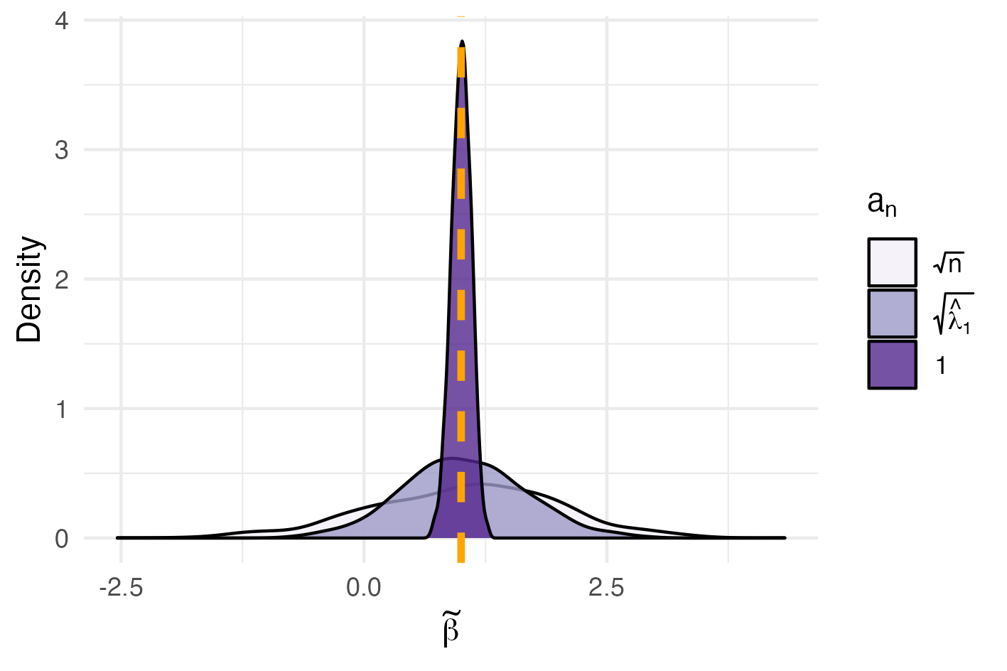
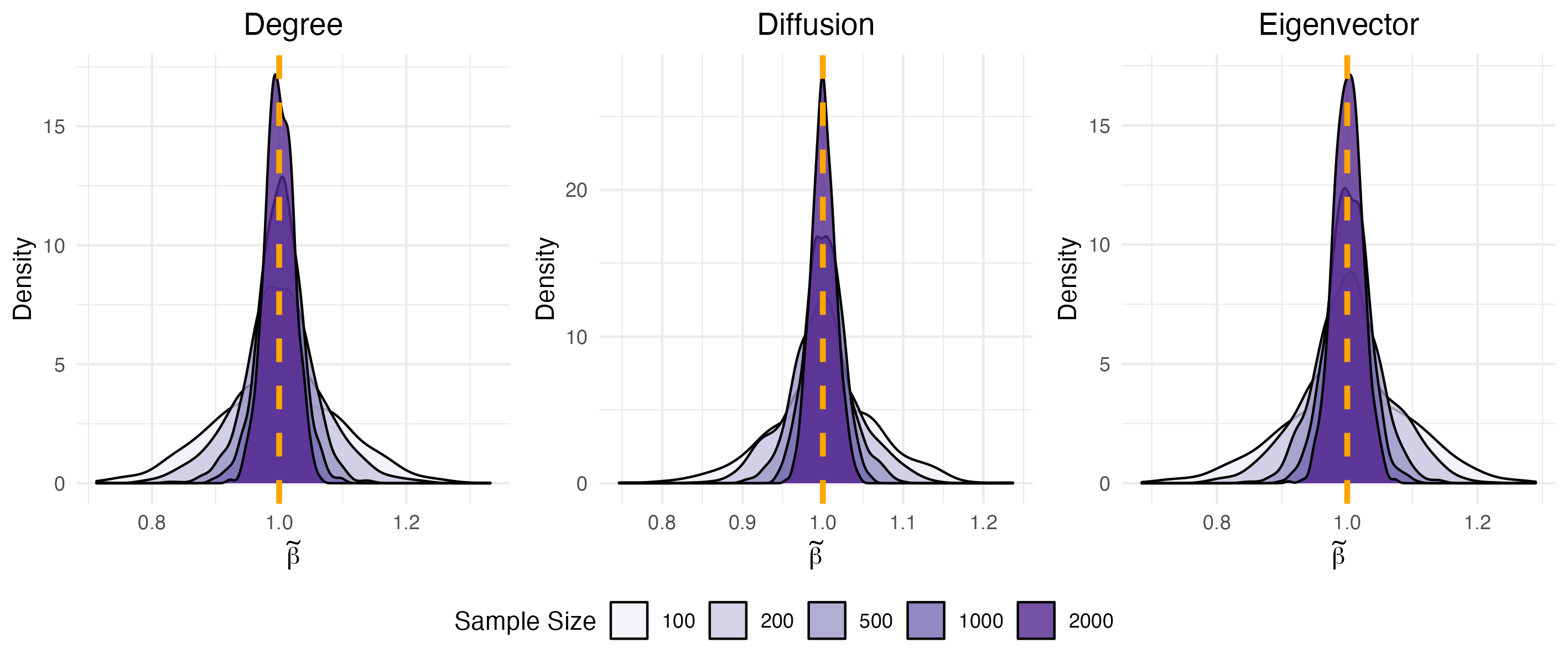
Figure 3: Distribution of $\tilde{\beta}^{(\infty)}$ for $n=100$, $p_{n}=1/n$ under various $a_{n}$. $\beta=1$ (orange dashed line).

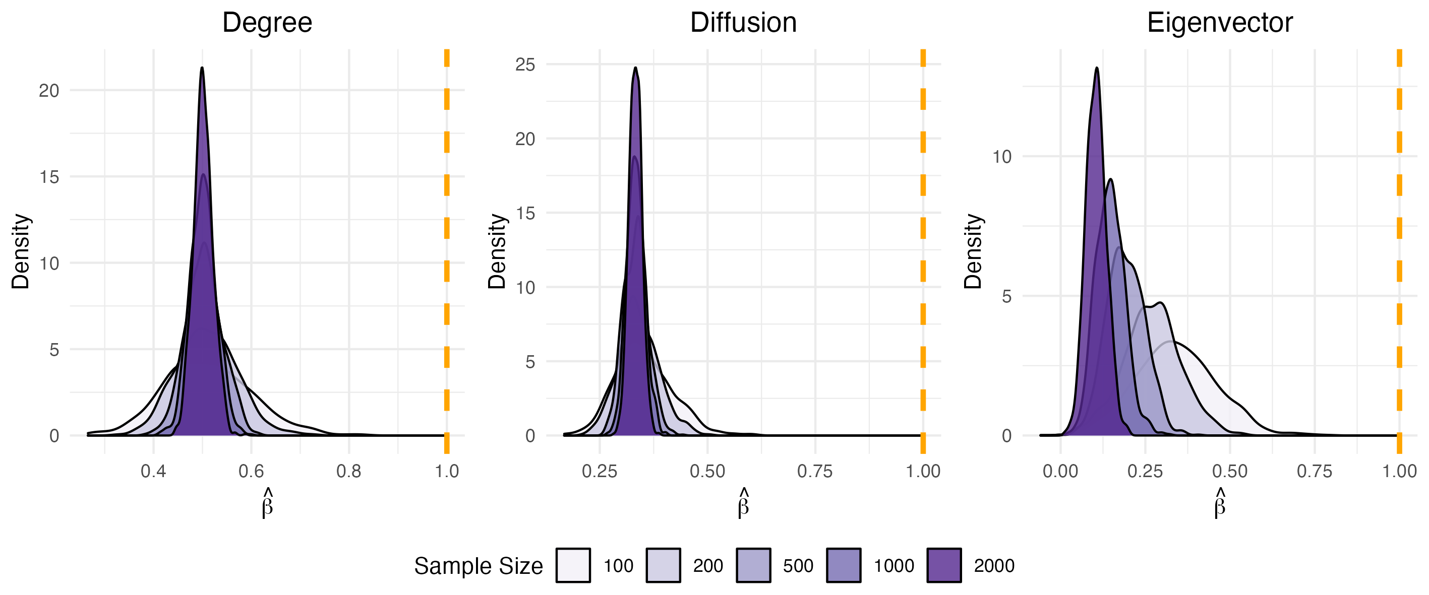
Figure 4: Distribution of $\tilde{\beta}^{(d)}$ for $p_{n}=1/n$. For $\tilde{\beta}^{(\infty)}$, $a_{n}=\sqrt{n}$. $\beta=1$ (orange dashed line).

Figure 5: Distribution of $\hat{\beta}^{(d)}$ for $p_{n}=1/n$. For $\tilde{\beta}^{(\infty)}$, $a_{n}=\sqrt{n}$. $\beta=1$ (orange dashed line).

We return to the first claim concerning consistency of $\tilde{\beta}^{(d)}$ when $p_{n}=1/n$. Figure 5 indeed shows the distribution of $\tilde{\beta}^{(d)}$ for each $n$. The estimators concentrate around $\beta$ as $n$ increases, in line with our result. However, Theorem 2 asserts that $\hat{\beta}^{(1)}$, $\hat{\beta}^{(T)}$ and $\hat{\beta}^{(\infty)}$ are all inconsistent when $p_{n}=1/n$. Their distributions, presented in Figure 5, concords with our result. Indeed, we see that $\hat{\beta}^{(1)}$ and $\hat{\beta}^{(T)}$ are attenuated by constant amount as $n\to\infty$, while $\hat{\beta}^{(\infty)}$ converges in probability to $0$.

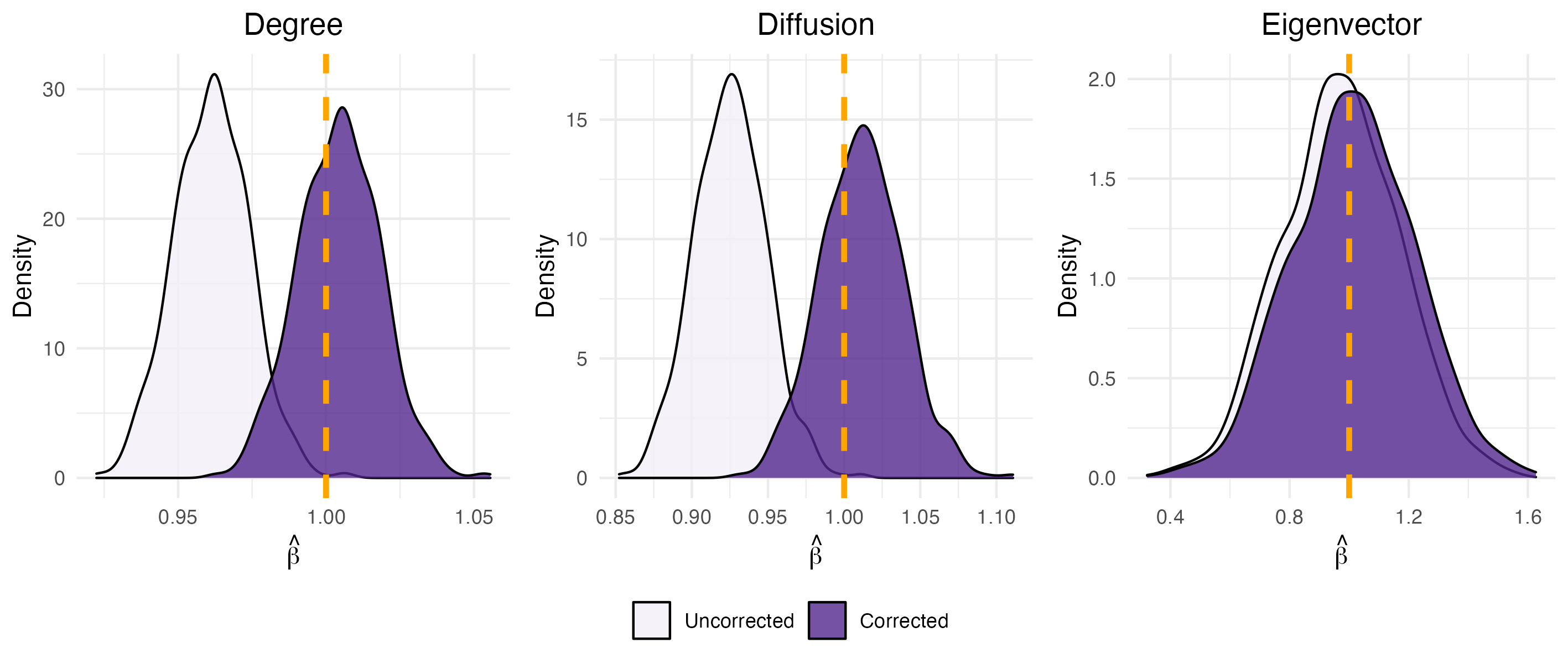
Figure 6: Distribution of $\hat{\beta}^{(d)}$ for $p_{n}=n^{-1}\sqrt{\log n/\log\log n}$. For $\tilde{\beta}^{(\infty)}$, $a_{n}=\sqrt{n}$. $\beta=1$ (orange dashed line).

Figure 7: Distributions of $\hat{\beta}^{(d)}$ and their bias corrected versions $\check{\beta}^{(d)}$ for $p_{n}=1/\sqrt{n}$. $\beta=1$ (orange dashed line).

Finally, we consider the case when $p_{n}=n^{-1}\sqrt{\frac{\log n}{\log\log n}}$. In this regime, $\hat{\beta}^{(1)}$ and $\hat{\beta}^{(T)}$ are consistent but $\hat{\beta}^{(\infty)}$ is not. We see suggestive evidence of this in Figure 7, where $\hat{\beta}^{(\infty)}$ is drifting further away from $\beta$ as $n$ increases. The opposite occurs with $\hat{\beta}^{(1)}$ and $\hat{\beta}^{(T)}$. Though the rate of convergence is slow, it is visible.

4.2 Bias Correction

Even in regime dense enough such that $\hat{\beta}^{(1)}$, $\hat{\beta}^{(T)}$ and $\hat{\beta}^{(\infty)}$ are consistent, they can still be subject to biases that affect their rates of convergence. This motivates the bias-corrected estimators in Definition 9. In this subsection, we study the effects of bias correction in the regime $p_{n}=1/\sqrt{n}$.

Figure 7 shows the distribution of the estimators when $n=500$. Here $a_{n}=\sqrt{\hat{\lambda}_{1}(\hat{A})}$. We see that bias correction is effective in correctly centering $\hat{\beta}^{(1)}$ and $\hat{\beta}^{(T)}$. The same is true for $\hat{\beta}^{(\infty)}$ though to a smaller extent, in line with claims in Corollary 4. Results for other values of $n$ are qualitatively similar.

4.3 Distributional Theory

Finally, we investigate the quality of the normal approximations proposed in Theorems 4 and 5. As before, we consider the regime $p_{n}=1/\sqrt{n}$. Figure 8 presents the distribution of test statistics (in purple) which our theorems predict have the standard normal distribution (in gray). We see that the two distributions are indeed close. It is also common for applied researcher to compute the usual $t$-statistic with heteroskedaticity consistent (robust) standard errors and conduct inference under the assumption that it has a standard normal distribution. For comparison, we include the distribution of the t-statistic (in lavender). Corollary 4 justifies the use of this statistic when $a_{n}=\sqrt{\hat{\lambda}_{1}(\hat{A})}$ but our theory for degree and diffusion centralities is based on a different statistic. Indeed, we see that the robust $t$-statistic can be quite far from the standard normal distribution in both location and dispersion. This suggests that our method would lead to more reliable tests.

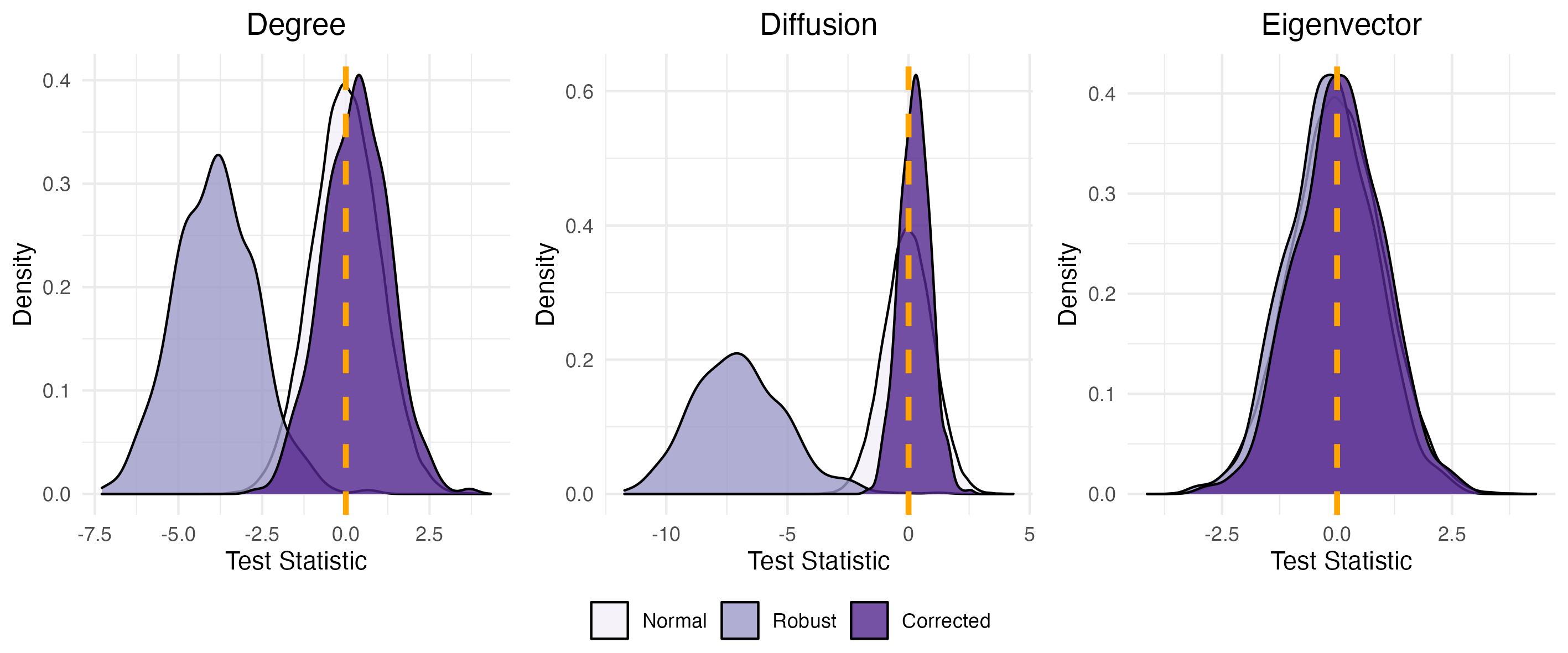
Figure 8: Distribution of the centered and scaled test statistics in Theorems 4 and 5. Robust refers to tests based on $t$-statistic with robust (heteroskedasticity consistent) standard errors.

We next examine the size and power of tests based on our distributional theory. We consider testing the hypothesis $H_{0}:\beta=\beta_{0}$ against $H_{1}:\beta\neq\beta_{0}$ at 5% level of significance. Table 1 presents size of the test when $\beta=1$ is correctly specified. For degree and diffusion centralities, our theory provides test statistics which differ from the robust $t$-statistic. As we see from the table, the test for degree controls size well. The test for diffusion centrality is more conservative. This is because our estimator $\hat{V}^{(T)}$ is upward-biased in finite sample when there are no other covariates. Tests for degree and diffusion centralities that are based on the robust $t$-statistic has Type I error over 50% across all sample sizes. For eigenvector centrality, our theory predicts that the robust $t$-statistic will perform well Indeed, it has size close to 5%. We also consider testing the hypothesis $\beta=0$. Power for this test is presented in Table 2. For this null hypothesis, our theory suggests the use of the robust $t$-statistic. Reassuringly, the tests all have power close to $1$. To understand how power changes as we vary the alternative hypothesis, we hone in on the case where $n=500$ and $p_{n}=1/\sqrt{n}$. Figure 9 presents the rejection probability of our test under various alternatives. We see that the our tests control size and have good power. Comparatively, tests based on the robust $t$-statistic have poor size control when $\beta\neq 0$. Furthermore, they can have poor power against particular alternatives owing to the bias. We conclude that our tests have desirable properties and are preferred to the test with robust $t$-statistic when networks are sparse and observed with noise.

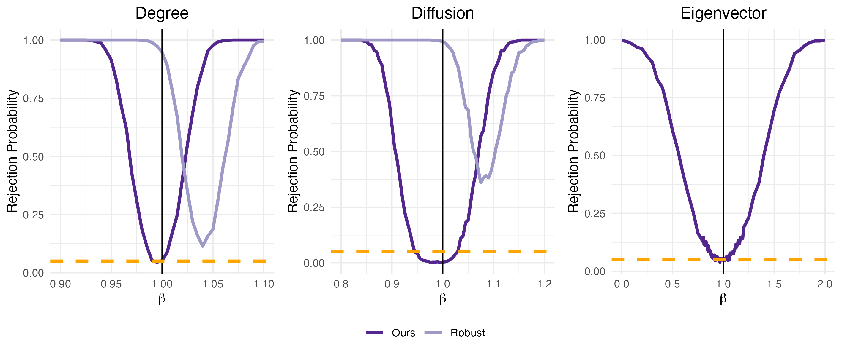
Figure 9: Power of the two-sided test of $H_{0}:\beta=1$ under various alternatives. Test at 5% level of significance (orange dashed line).

$p_{n}$	Statistic		Sample Size
			100		200		500		1000		2000
0.1	Degree	Ours	0.055		0.052		0.067		0.062		0.065
		Robust	0.573		0.645		0.680		0.662		0.670
	Diffusion	Ours	0.010		0.004		0.007		0.003		0.004
		Robust	0.859		0.883		0.883		0.868		0.897
	Eigenvector		0.054		0.060		0.046		0.052		0.046
$n^{-1/3}$	Degree	Ours	0.066		0.065		0.067		0.058		0.065
		Robust	0.286		0.422		0.556		0.701		0.778
	Diffusion	Ours	0.006		0.001		0.002		0.008		0.003
		Robust	0.621		0.729		0.805		0.888		0.933
	Eigenvector		0.045		0.055		0.050		0.056		0.038
$n^{-1/2}$	Degree	Ours	0.072		0.049		0.051		0.037		0.062
		Robust	0.580		0.761		0.944		0.993		0.999
	Diffusion	Ours	0.015		0.009		0.005		0.001		0.004
		Robust	0.863		0.944		0.993		1.000		1.000
	Eigenvector		0.053		0.049		0.036		0.067		0.056

Table 1: Size of 5% level two-sided tests when $\beta=1$ is correctly specified. Robust refers to tests based on $t$-statistic with robust (heteroskedasticity consistent) standard errors.

$p_{n}$	Statistic	Sample Size
		100		200		500		1000		2000
0.1	Degree	1.000		1.000		1.000		1.000		1.000
	Diffusion	1.000		1.000		1.000		1.000		1.000
	Eigenvector	0.880		0.993		1.000		1.000		1.000
$n^{-1/3}$	Degree	1.000		1.000		1.000		1.000		1.000
	Diffusion	1.000		1.000		1.000		1.000		1.000
	Eigenvector	0.994		1.000		1.000		1.000		1.000
$n^{-1/2}$	Degree	1.000		1.000		1.000		1.000		1.000
	Diffusion	1.000		1.000		1.000		1.000		1.000
	Eigenvector	0.860		0.972		0.997		1.000		1.000

Table 2: Power of 5% level two-sided tests of $H_{0}:\beta=0$ when $\beta=1$. Under this $H_{0}$, the our test statistics is the usual $t$-statistic with robust (heteroskedasticity-consistent) standard errors.

5 Empirical Demonstration

In this section, we demonstrate the relevance of our theoretical findings via an application inspired by De Weerdt and Dercon (2006). In the developing world, social insurance is an important mechanism for smoothing consumption, because of restricted access to formal credit markets (Rosenzweig 1988; Udry 1994; Fafchamps and Lund 2003; Kinnan and Townsend 2012, among many others). De Weerdt and Dercon (2006) examines the case of Nyakatoke, a village with 120 households in rural Tanzania, and find that social insurance helps households to smooth consumption following health shocks. The data they use comprises five rounds of panel data on household consumption, illness among other covariates, collected from February to December 2000. The authors also had access to social network data collected during the first round of the survey, in which households were asked for the identities of those who they depend on or depend on them for help. The authors then regress a household’s change in consumption following illness on the mean consumption of their network neighbors, finding evidence of positive co-movements.

Another way to demonstrate the effect of social insurance on consumption smoothing could be to regress variance in consumption on network centrality measures. Specifically, the regression:

$$Y_{i}=\beta C^{(d)}_{i}+\varepsilon_{i}$$

where $Y_{i}$ is variance in food expenditure and $C^{(d)}_{i}$ is a centrality measure. The above regression could be preferred to the authors’ specification if we are unsure about the covariates that reflect social assistance. For example, it might be a household’s stock of savings that co-move with the decision to lend to their friends, rather than their own consumption. We might also be interested in more complex patterns of assistance, which could be summarized in an appropriate centrality measure, but which might not be tractable with covariates.

The above regression requires information on network of social insurance, in which each entry $A_{ij}$ records the probability $i$ lends money to $j$ over the survey period. We can consider obtaining proxies for this network using one of the following:

• Unilateral Social (US). $\hat{A}_{ij}=1$ if either $i$ or $j$ names the other household as a party that they could depend on or which depends on them for help.

• Bilateral Social (BS). $\hat{A}_{ij}=1$ only if both $i$ and $j$ names the other household as a party that they could depend on or which depends on them for help.

• Unilateral Financial (UF). $\hat{A}_{ij}=1$ if either $i$ or $j$ lends money to the other at least once over the survey period.

The authors study US and BS. We also consider UF since self-reported loan data is available. The networks are plotted in Figure 10 and the degree distributions are described in Table 3. In a village with $n=120$ households, mean degree in all three networks are less than $11$. We might therefore be concerned that $np_{n}\prec\sqrt{n}$. By construction, US is much less dense than BS. Due to the availability of five panels, UF is denser than the other two.

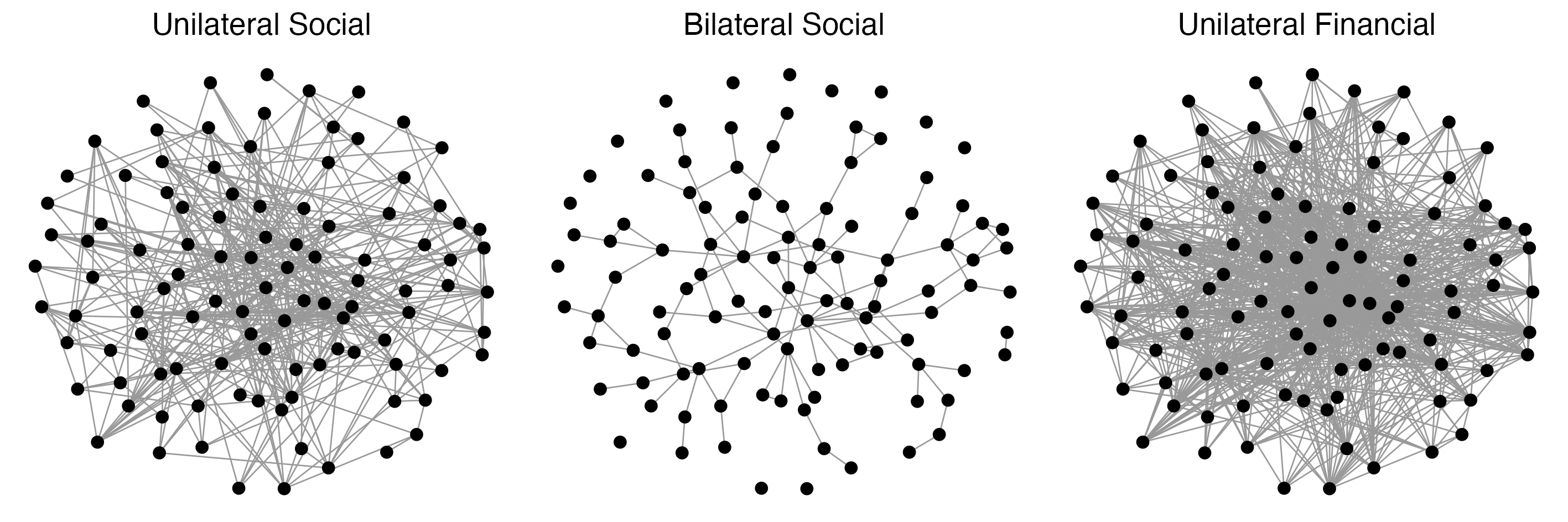
Figure 10: Social and Financial networks in Nyakatoke.

($n=119$)	Mean	Median	Min	Max
Unilateral Social	8.10	7	0	31
Bilateral Social	2.32	2	0	10
Unilateral Transfer	10.48	8	1	77

Table 3: Degree distributions of various networks in Nyakatoke.

Regression results are presented in Table 4. In this exercise, $a_{n}=\sqrt{\lambda_{1}(\hat{A})}$, $\delta=1/\sqrt{\lambda_{1}(\hat{A})}$ and $T=2$. We first note that estimated attenuation factor is the smallest (i.e. furthest from 1) in the sparsest network BS. This is in line with our result that bias is $O_{p}(n^{-1}p_{n}^{-1})$. Diffusion centrality is generally estimated to be less attenuated, because $\delta$ is small $(\approx 0.2)$. As the last column shows, bias correction can lead to substantially different estimates. Table 4 also presents $p$-values for tests of the two-sided hypothesis that $\beta^{(d)}=0$. Centrality statistics on BS appears to be more predictive of the variance in food consumption than that on US and UF. This highlights that researchers should not choose their network proxies on the criteria of sparsity alone. In the case of Nyakatoke, evidence suggests that US reflects “desire to link”, rather than actual risk-pooling (Comola and Fafchamps 2014), such that US is a noisier proxy than BS. By the same account, the large number of discrepancies between reporting by borrowers and lenders of the same loan suggests that the loan data is subject to severe mis-reporting (Comola and Fafchamps 2017), rendering it an equally poor proxy. Among the centrality statistics on BS, eigenvector has the least predictive power by far. We reiterate our warning that eigenvector centrality is less robust to sparsity than degree and diffusion, such that the $p$-values might reflect the poor statistical properties of the measure, rather than its lack of economic significance.

		Estimate	p-value	Atten.	Bias Corr.
Unilateral Social	Degree	-1064	0.67	0.91	-1172
	Diffusion	-4274	0.77	1.00	-4292
	Eigenvector	-12353	0.86	0.91	-13548
Bilateral Social	Degree	-11604	0.06	0.74	-15592
	Diffusion	-23672	0.16	0.94	-25212
	Eigenvector	-10543	0.93	0.78	-13434
Unilateral Financial	Degree	-412	0.70	0.96	-429
	Diffusion	-4559	0.74	1.00	-4561
	Eigenvector	-15040	0.77	0.96	-15699

Table 4: Regression results for various networks. Estimate is $\hat{\beta}^{(d)}$. $p$-value is for the two-sided test that $H_{0}:\beta=0$. Atten. is the estimated attenuation factor of $\hat{\beta}^{(d)}$ (i.e. $1-\hat{B}^{(d)}$). Bias Corr. presents the bias corrected estimates, $\check{\beta}^{(d)}$.

Finally, we present one-sided confidence intervals for values of $\beta^{(d)}$ based on our results. These are useful for putting bounds on parameter values. In our example, a lower bound could be intuitively interpreted as the limits to informal risk-sharing, a quantity which could be useful for policymakers deciding whether or not to provide agricultural insurance. We focus on BS since it appears to be the only informative network. Results for degree and diffusion are presented in Table 5. Our confidence intervals leads to tighter lower bound than the those based on the robust $t$-statistic. Results for eigenvector are omitted since our theory is based on the usual robust $t$-statistic.

		90%	95%	99%
Degree	Ours	(-18835, $\infty$)	(-20015, $\infty$)	(-22680, $\infty$)
	Robust	(-25050, $\infty$)	(-28862, $\infty$)	(-36012, $\infty$)
Diffusion	Ours	(-34715, $\infty$)	(-38867, $\infty$)	(-50112, $\infty$)
	Robust	(-56938, $\infty$)	(-66368, $\infty$)	(-84058, $\infty$)

Table 5: One-sided confidence intervals for degree and diffusion.

6 Conclusion

In this paper, we studied the properties of linear regression on degree, diffusion and eigenvector centrality when networks are sparse and observed with error. We show that these issues threaten the consistency of OLS estimators and characterize the amount of sparsity at which inconsistency occurs. In doing so, we find that eigenvector centrality is less robust to sparsity than the others and that the statistical properties of the corresponding regression is sensitive to the scaling.

Additionally, we show that an asymptotic bias arises whenever the true slope parameter is not $0$ and that the bias can be of larger order than the variance, so that bias correction is necessary to obtain a non-degenerate limiting distribution from the OLS estimator. Finally, we provide estimators for the bias and variance which, together with our central limit theorem, facilitates inference under sparsity and measurement error. We confirm our theoretical results via simulations, which suggest that our approximation result works better for estimation and inference when networks are sparse, particularly when compared to the use of robust standard errors and the associated $t$-statistics. Finally, we demonstrate the relevance of our theoretical results by studying the social insurance network in Nyakatoke, Tanzania.

In sum, our results suggest that applied researchers view their results with caution when applying OLS to sparse, noisy networks. Specifically, comparing the statistical significance of eigenvector centrality with degree or diffusion may yield misleading conclusions since they differ not only in economic significance but also statistical properties. Provided that the networks are not too sparse, the usual $t$-test is valid for null hypothesis that the slope parameter is $0$. However, alternative inference procedures will be necessary for other null hypotheses. Additionally, there may be scope for improving estimation by the use of bias-corrected estimators. Estimation and inference under extreme sparsity remains an open question, though as (Le et al. 2017) show, parametric models such as the Stochastic Block Model may point to a way forward.

Appendices

Appendix A Proofs

We maintain Assumptions 1, 2 and 3 throughout the entire section. Without loss of generality, let $f(u,v)=f(v,u)$ and the $f(u,u)=0$. Further define:

$$W=\int_{[0,1]^{2}}f(u,v)\,dudv~{}.$$

We state below a convenient lemma:

Lemma 1 (Concentration in Spectral Norm).

Suppose Assumptions 1 and 2 hold. Let $\nu\in(0,1)$. Then with probability at least $1-\exp\left(-n^{2}p_{n}^{2}\sqrt{k\frac{\log n}{\log\log n}}\right)$

$$\left\lVert A-\hat{A}\right\rVert\leq k\left(np_{n}\right)^{(1+\nu)/2}\left(\frac{\log n}{\log\log n}\right)^{(1-\nu)/4}$$

where $k$ is a universal constant. In other words,

$$\left\lVert A-\hat{A}\right\rVert=O_{p}\left(\left(np_{n}\right)^{(1+\nu)/2}\left(\frac{\log n}{\log\log n}\right)^{(1-\nu)/4}\right)~{}.$$ (9)

A.1 Proof of Theorem 1

In the setting with no measurement error, we write:

$$\tilde{\beta}^{(d)}=\frac{\sum_{i=1}^{n}Y_{i}C^{(d)}_{i}}{\sum_{i=1}^{n}\left(C^{(d)}_{i}\right)^{2}}=\beta+\frac{\sum_{i=1}^{n}C^{(d)}_{i}\varepsilon_{i}}{\sum_{i=1}^{n}\left(C^{(d)}_{i}\right)^{2}}~{}.$$

We first show that OLS is consistent when the lower bounds in the Theorem obtains. Start with degree:

$$\sum_{i=1}^{n}C^{(1)}_{i}\varepsilon_{i} =\sum_{i=1}^{n}\sum_{j=1}^{n}p_{n}f(U_{i},U_{j})\varepsilon_{i}$$

$$=\frac{p_{n}}{2}{n\choose 2}\cdot\frac{1}{{n\choose 2}}\sum_{i=1}^{n}\sum_{j=1}^{n}f(U_{i},U_{j})\varepsilon_{i}+f(U_{j},U_{i})\varepsilon_{j}$$ (10)

$$=O_{p}\left(n^{3/2}p_{n}\right)~{},$$

In the last equality, we use our assumption that $E[\varepsilon_{i}|U_{i}]=0$ and $E[\varepsilon_{i}^{2}|U_{i}]\leq\sigma^{2}<\infty$, so that

$$\sqrt{n}\cdot\frac{1}{{n\choose 2}}\sum_{i=1}^{n}\sum_{j=1}^{n}f(U_{i},U_{j})\varepsilon_{i}+f(U_{j},U_{i})\varepsilon_{j}\overset{d}{\to}\text{N}(0,\gamma)$$

for some $\gamma>0$ by the standard CLT for U-statistics (e.g. Theorem 12.3 in Van der Vaart 2000). Similarly,

$$\sum_{i=1}^{n}\left(C^{(1)}_{i}\right)^{2} =\sum_{i=1}^{n}\left(\sum_{j=1}^{n}p_{n}f(U_{i},U_{j})\right)^{2}$$

$$=p_{n}^{2}\sum_{i=1}^{n}\sum_{j=1}^{n}\sum_{k=1}^{n}f(U_{i},U_{j})f(U_{i},U_{k})$$ (11)

$$=p_{n}^{2}{n\choose 3}\cdot\frac{1}{{n\choose 3}}\sum_{k=1}^{n}f(U_{i},U_{j})f(U_{i},U_{k})=O_{p}(n^{3}p_{n}^{2})$$

By the LLN for U-statistics,

$$\frac{1}{{n\choose 3}}\sum_{k=1}^{n}f(U_{i},U_{j})f(U_{i},U_{k})\overset{p}{\to}\gamma$$

Next, note that $\gamma>0$. Let $k$ and $B_{k}$ be such that $f(u,v)>1/k$ for all $(u,v)\in B_{k}$. Our assumption $W>0$ ensures that there exists $k$ such that $P_{k}:=\int_{[0,1]^{2}}\mathbf{1}_{B_{k}}\,dudv>0$. Then,

$$\gamma =\int_{[0,1]^{3}}f(u_{1},u_{2})f(u_{1},u_{3})\,du_{1}du_{2}du_{3}$$

$$\geq\int_{\pi_{1}(B_{k})\times\pi_{2}(B_{k})\times\pi_{2}(B_{k})}k^{-2}\,du_{1}du_{2}du_{3}\geq P_{k}^{2}k^{-2}>0$$

where $\pi_{j}(B_{k})$ denotes the projection of $B_{k}$ onto the $j^{\text{th}}$ coordinate. Hence, we have consistency if $n^{3/2}p_{n}\to\infty$. If $n^{3/2}p_{n}\approx 1$, the $\tilde{\beta}^{(1)}-\beta^{(1)}$ converges to a normal distribution. If $n^{3/2}p_{n}\prec 1$, $\tilde{\beta}^{(1)}-\beta^{(1)}$ diverges. Hence, we have consistency if and only if $n^{3/2}p_{n}\to\infty$

Remark 6.

Note that the analysis for normalized degree is similar, except that the numerator is now of order $n^{1/2}p_{n}$ while the denominator is of order $np^{2}_{n}$. Consistency with the normalized degree thus require $n^{1/2}p_{n}\to\infty$ as noted in Remark LABEL:remark--normalized_degree.

Next, consider diffusion centrality. Note that:

$$\sum_{i=1}^{n}C^{(T)}_{i}\varepsilon_{i} =\sum_{t=1}^{T}\delta^{t}\cdot\iota_{n}^{\prime}A^{t}\varepsilon\quad,\quad\sum_{i=1}^{n}\left(C^{(T)}_{i}\right)^{2}=\sum_{t=1}^{T}\delta^{2t}\cdot\iota_{n}^{\prime}A^{2t}\iota_{n}~{}.$$

We will identify the dominant terms in the numerator and denominator respectively in each regime of $p_{n}$. For $t\geq 2$, write:

$$\left[A^{t}\right]_{ij}=p_{n}^{t}\sum_{k_{1}=1}^{n}\sum_{k_{2}=1}^{n}\cdots\sum_{k_{t-1}=1}^{n}f(U_{i},U_{k_{1}})f(U_{k_{1}},U_{k_{2}})\cdots f(U_{k_{t-1}},U_{j})~{}.$$

Applying the CLT for U-statistics as before, we have that

$$\iota_{n}^{\prime}A^{t}\varepsilon =p_{n}^{t}\sum_{i=1}^{n}\sum_{j=1}^{n}\sum_{k_{1}=1}^{n}\sum_{k_{2}=1}^{n}\cdots\sum_{k_{t-1}=1}^{n}f(U_{i},U_{k_{1}})f(U_{k_{1}},U_{k_{2}})\cdots f(U_{k_{t-1}},U_{j})\varepsilon_{j}=O_{p}\left(p_{n}^{t}n^{t+1/2}\right)~{}.$$

Similarly,

$$\iota_{n}^{\prime}A^{2t}\iota_{n} =p_{n}^{2t}\sum_{i=1}^{n}\sum_{j=1}^{n}\sum_{k_{1}=1}^{n}\sum_{k_{2}=1}^{n}\cdots\sum_{k_{2t-1}=1}^{n}f(U_{i},U_{k_{1}})f(U_{k_{1}},U_{k_{2}})\cdots f(U_{k_{2t-1}},U_{j})=O_{p}\left(p_{n}^{2t}n^{2t+1}\right)~{}.$$ (12)

Next, suppose $np_{n}\succ 1$. Then the dominant terms in the numerator and denominator are of order $O(p_{n}^{T}n^{T+1/2})$ and $O(p_{n}^{2T}n^{2T+1})$ respectively. As such,

$$\tilde{\beta}^{(T)}-\beta^{(T)}=O_{p}(p_{n}^{-T}n^{-T-1/2})=o_{p}(1)~{}.$$

Suppose instead that $np_{n}\approx 1$. Then, all terms in the numerator are of the same order. The same is true for the denominator. As before, $\tilde{\beta}^{(T)}-\beta^{(T)}=O_{p}(n^{-1/2})=o_{p}(1)$.

Finally, suppose $np_{n}\prec 1$. In this regime, diffusion is equivalent to degree to a first order. The dominant terms in the numerator and denominator are of order $O(p_{n}n^{3/2})$ and $O(p_{n}^{2}n^{3})$ respectively. Then, as before, we obtain consistency if and only if $n^{3/2}p_{n}\to\infty$.

Lastly, consider eigenvector centrality. Given our assumptions, $v_{1}(A)$ is well-defined with high probability. Next note that by construction, $\sum_{i=1}^{n}\left(C^{(\infty)}_{i}\right)^{2}=a_{n}^{2}~{}.$ Furthermore, by our assumptions,

$$E\left[\sum_{i=1}^{n}C^{(d)}_{i}\varepsilon_{i}\,\big{\lvert}\,U\right]=\sum_{i=1}^{n}C^{(d)}_{i}E\left[\varepsilon_{i}\,\big{\lvert}\,U\right]=0$$

$$\text{Var}\left[\sum_{i=1}^{n}C^{(d)}_{i}\varepsilon_{i}\,\big{\lvert}\,U\right]=\sum_{i=1}^{n}\left(C^{(d)}_{i}\right)^{2}\text{Var}\left[\varepsilon_{i}\,\big{\lvert}\,U\right]\leq a_{n}^{2}\bar{\sigma}^{2}~{}.$$

As such,

$$\text{Var}\left[\tilde{\beta}^{(\infty)}-\beta^{(\infty)}\right]\leq\frac{\bar{\sigma}^{2}}{a_{n}^{2}}\to 0\mbox{ if }a_{n}\to\infty~{}.$$

Thus, $a_{n}\to\infty$ implies that $\tilde{\beta}^{(\infty)}\overset{L_{2}}{\to}\beta^{(\infty)}$.

Necessity follows from the counterexample in our main text, reproduced here for completeness. Suppose $f=p_{n}\cdot 1$ so that $A=p_{n}\iota_{n}\iota_{n}^{\prime}$. Then $C^{(\infty)}(A)=a_{n}\iota_{n}/\sqrt{n}$. Hence,

$$\tilde{\beta}^{(\infty)}=\frac{\sqrt{n}}{a_{n}}\cdot\frac{Y^{\prime}\iota_{n}}{\iota_{n}^{\prime}\iota_{n}}=\beta^{(\infty)}+\frac{1}{a_{n}\sqrt{n}}\sum_{i=1}^{n}\varepsilon_{i}~{}.$$

Under our assumptions, $\frac{1}{\sqrt{n}}\sum_{i=1}^{n}\varepsilon_{i}\overset{d}{\to}N(0,\text{Var}[\varepsilon_{i}])$. For $\tilde{\beta}^{(\infty)}$ to be consistent for $\beta^{(\infty)}$, it is therefore necessary for $a_{n}\to\infty$.

A.2 Proof of Theorem 2

We first write:

$$\hat{\beta}^{(d)}=\beta^{(d)}+\beta^{(d)}\frac{\left(\hat{C}^{(d)}\right)^{\prime}\left(C^{(d)}-\hat{C}^{(d)}\right)}{\left(\hat{C}^{(d)}\right)^{\prime}\hat{C}^{(d)}}+\frac{\left(\hat{C}^{(d)}\right)^{\prime}\varepsilon}{\left(\hat{C}^{(d)}\right)^{\prime}\hat{C}^{(d)}}$$

For convenience, denote

$$\hat{A}_{ij}=p_{n}f(U_{i},U_{j})+\xi_{ij}\quad,\quad E[\xi_{ij}\,|\,U_{i},U_{j}]=0~{}.$$

Also let $\xi_{i}=\sum_{j=1}^{n}\xi_{ij}=\sum_{j\neq i}\xi_{ij}$ and $\xi=(\xi_{1},...,\xi_{n})^{\prime}$. Finally, let $\boldsymbol{\xi}$ by the $n\times n$ matrix with $(i,j)^{\text{th}}$ entry $\xi_{ij}$. Note that $\xi=\boldsymbol{\xi}\iota_{n}$. By Assumption 2, $\xi_{ij}\perp\!\!\!\perp\varepsilon_{k}\,|\,U$ for all $i,j,k$.

A.2.1 Degree

We first show that $np_{n}\succ 1$ is sufficient for consistency of $\hat{\beta}^{(1)}$. Using our new notation, the numerator is:

$$\left(\hat{C}^{(1)}\right)^{\prime}\varepsilon=C^{(1)}\varepsilon+\xi^{\prime}\varepsilon~{}.$$

By conditional independence of $\xi$ and $\varepsilon$, $E\left[\xi^{\prime}\varepsilon\right]=0$

$$\text{Var}\left[\xi^{\prime}\varepsilon\,\lvert\,U\right] =\text{Var}\left[2\sum_{i=1}^{n}\sum_{j>i}\xi_{ij}\varepsilon_{i}\,\bigg{\lvert}\,U\right]=4\sum_{i=1}^{n}\text{Var}\left[\varepsilon_{i}\sum_{j>i}\xi_{ij}\,\bigg{\lvert}\,U\right]$$

$$=4\sum_{i=1}^{n}\left(E\left[\varepsilon^{2}_{i}\,|\,U\right]\sum_{j>i}E\left[\xi^{2}_{ij}\,|\,U\right]\right)$$

$$\leq 2\bar{\sigma}^{2}\sum_{i=1}^{n}\sum_{j>i}p_{n}f(U_{i},U_{j})\left(1-p_{n}f(U_{i},U_{j})\right)$$

$$\leq 2\bar{\sigma}^{2}\sum_{i=1}^{n}\sum_{j>i}p_{n}f(U_{i},U_{j})$$

Taking expectations over $U$, we have that

$$\text{Var}\left[\xi^{\prime}\varepsilon\right]\leq 2\bar{\sigma}^{2}n^{2}p_{n}\cdot W\quad\Rightarrow\quad\xi^{\prime}\varepsilon=O_{p}(n{p_{n}}^{1/2})$$

Given Equation (A.1), $C^{(1)}\varepsilon=O_{p}(n^{3/2}p_{n})$ is thus dominant in the numerator if $np_{n}\succ 1$.

Next, consider the denominator, which has the form:

$$\left(\hat{C}^{(1)}\right)^{\prime}\hat{C}^{(1)}=\left(C^{(1)}\right)^{\prime}C^{(1)}+2\left(C^{(1)}\right)^{\prime}\xi+\xi^{\prime}\xi~{}.$$

We bound the last term in $L_{1}$-norm. Observe that it has conditional expectation:

$$E\left[\xi^{\prime}\xi\,|\,U\right] =E\left[\sum_{i=1}^{n}\left(\sum_{j\neq i}\xi_{ij}\right)^{2}\,\bigg{\lvert}\,U\right]=\sum_{i=1}^{n}\sum_{j\neq i}\sum_{k\neq i}E\left[\xi_{ij}\xi_{ik}\,\big{\lvert}\,U\right]$$

$$=\sum_{i=1}^{n}\sum_{j\neq i}E\left[\xi^{2}_{ij}\,\big{\lvert}\,U\right]\leq\sum_{i=1}^{n}\sum_{j\neq i}p_{n}f(U_{i},U_{j})~{}.$$

Taking expectations over $U$,

$$E\left[\xi^{\prime}\xi\right]\leq n^{2}p_{n}\cdot W\quad\Rightarrow\quad\xi^{\prime}\xi=O_{p}(n^{2}p_{n})~{}.$$ (13)

Next, consider the middle term, which we will bound in $L_{2}$-norm. Write

$$E\left[\left(\left(C^{(1)}\right)^{\prime}\xi\right)^{2}\,\bigg{\lvert}\,U\right] =E\left[\sum_{i=1}^{n}\sum_{j=1}^{n}C^{(1)}_{i}\xi_{i}C^{(1)}_{j}\xi_{j}\,\bigg{\lvert}\,U\right]$$

$$=E\left[\sum_{i=1}^{n}C^{(1)}_{i}\xi_{i}C^{(1)}_{i}\xi_{i}\,\bigg{\lvert}\,U\right]+E\left[\sum_{i=1}^{n}\sum_{j\neq i}^{n}C^{(1)}_{i}\xi_{i}C^{(1)}_{j}\xi_{j}\,\bigg{\lvert}\,U\right]~{}.$$

Note that

$$E\left[\sum_{i=1}^{n}\sum_{j\neq i}^{n}C^{(1)}_{i}\xi_{i}C^{(1)}_{j}\xi_{j}\,\bigg{\lvert}\,U\right] =\sum_{i=1}^{n}\sum_{j\neq i}^{n}C^{(1)}_{i}C^{(1)}_{j}E\left[\xi_{i}\xi_{j}\,\big{\lvert}\,U\right]=\sum_{i=1}^{n}\sum_{j\neq i}^{n}C^{(1)}_{i}C^{(1)}_{j}E\left[\xi^{2}_{ij}\,\big{\lvert}\,U\right]$$

$$\leq\sum_{i=1}^{n}\sum_{j\neq i}^{n}C^{(1)}_{i}C^{(1)}_{j}p_{n}f(U_{i},U_{j})$$

$$=\sum_{i=1}^{n}\sum_{k=1}^{n}\sum_{l=1}^{n}\sum_{j\neq i}^{n}p_{n}^{3}f(U_{i},U_{k})f(U_{i},U_{l})f(U_{i},U_{j})$$

The second equality above follows form the fact that when $i\neq j$, $E[\xi_{ik}\xi_{jl}\,|\,U]=0$ unless $k=j$ and $l=i$. Furthermore,

$$E\left[\sum_{i=1}^{n}C^{(1)}_{i}\xi_{i}C^{(1)}_{i}\xi_{i}\,\bigg{\lvert}\,U\right] \leq\sum_{i=1}^{n}\left(C_{i}^{(1)}\right)^{2}E\left[\xi^{2}_{i}\,\big{\lvert}\,U\right]=\sum_{i=1}^{n}\left(C_{i}^{(1)}\right)^{2}E\left[\sum_{j\neq i}\xi_{ij}^{2}\,\bigg{\lvert}\,U\right]$$

$$\leq\sum_{i=1}^{n}\left(C_{i}^{(1)}\right)^{2}\sum_{j\neq i}p_{n}f(U_{i},U_{j})$$

$$\leq\sum_{i=1}^{n}\sum_{k=1}^{n}\sum_{l=1}^{n}p_{n}^{2}f(U_{i},U_{k})f(U_{i},U_{l})\sum_{j\neq i}p_{n}f(U_{i},U_{j})$$

Taking expectation over two displays above,

$$E\left[\left(\left(C^{(1)}\right)^{\prime}\xi\right)^{2}\right] =O(n^{4}p_{n}^{3})\quad\Rightarrow\quad\left(C^{(1)}\right)^{\prime}\xi=O_{p}(n^{2}p_{n}^{3/2})~{}.$$ (14)

By Equation (A.1), $\left(C^{(1)}\right)^{\prime}C^{(1)}=O_{p}(n^{3}p_{n}^{2})$. Putting the rates we derived together, the denominator is

$$\left(\hat{C}^{(1)}\right)^{\prime}\hat{C}^{(1)}=O_{p}(n^{3}p_{n}^{2})+O_{p}(n^{2}p_{n}^{3/2})+O_{p}(n^{2}p_{n})~{}.$$ (15)

Hence, $np_{n}\succ 1$ implies that

$$\frac{\left(\hat{C}^{(1)}\right)^{\prime}\varepsilon}{\left(\hat{C}^{(1)}\right)^{\prime}\hat{C}^{(1)}}\overset{p}{\to}0~{}.$$

It remains to note that

$$\left(\hat{C}^{(1)}\right)^{\prime}\left(C^{(1)}-\hat{C}^{(1)}\right)=\left({C}^{(1)}\right)^{\prime}\xi+\xi^{\prime}\xi$$

so that by the rates in (13), (14) and (15),

$$\beta^{(d)}\frac{\left(\hat{C}^{(d)}\right)^{\prime}\left(C^{(d)}-\hat{C}^{(d)}\right)}{\left(\hat{C}^{(d)}\right)^{\prime}\hat{C}^{(d)}}=O_{p}(n^{-1}p_{n}^{-1})\overset{p}{\to}0~{}.$$

We can loosely write the above results as

$$\hat{\beta}^{(1)}-\beta^{(1)}\approx\frac{n^{2}p_{n}^{3/2}+n^{2}p_{n}}{n^{3}p_{n}^{2}+n^{2}p_{n}^{3/2}+n^{2}p_{n}}+\frac{n^{3/2}p_{n}+np_{n}^{1/2}}{n^{3}p_{n}^{2}+n^{2}p_{n}^{3/2}+n^{2}p_{n}}$$

As such, $\hat{\beta}^{(1)}$ is consistent for $\beta^{(1)}$ if $np_{n}\succ 1$.

Suppose instead that $n^{-2}\prec p_{n}\prec n^{-1}$. By our rate calculations, we can write

$$\hat{\beta}^{(1)}-\beta^{(1)}=-\beta^{(1)}\cdot\frac{\xi^{\prime}\xi+o_{p}(n^{2}p_{n})}{\xi^{\prime}\xi+o_{p}(n^{2}p_{n})}+o_{p}(1)$$

In other words, $\hat{\beta}^{(1)}\overset{p}{\to}0$. Finally, if $p_{n}\prec n^{-2}$, we $\hat{\beta}^{(1)}-\beta^{(1)}$,

$$\hat{\beta}^{(1)}=\frac{\xi^{\prime}\varepsilon}{\xi^{\prime}\xi}+o_{p}(1)=O_{p}(n^{-2}p_{n}^{-1})$$

diverges in probability.

A.2.2 Diffusion Centrality

Diffusion centrality is comprised of terms of the form:

$$\hat{A}^{t}=\left(A+\boldsymbol{\xi}\right)^{t}=\sum_{B\in\tilde{\mathbf{B}}}B$$

Here, $\tilde{\mathbf{B}}=\left\{A,\boldsymbol{\xi}\right\}^{t}$. $B$ is a mixed product of $A$ and $\boldsymbol{\xi}$, and will be the central object of our analysis. For convenience, define:

Definition 10 (Mixed Product of Order $t$).

A mixed product of order $t$ is a term of the form $B=\prod_{j=1}^{t}B_{j}$ where $B_{j}\in\left\{A,\boldsymbol{\xi}\right\}$. Suppose $B_{j}=\boldsymbol{\xi}$ for $\tau\geq 0$ number of $j$’s. We will also say that the order of $\boldsymbol{\xi}$ in $B$ is $\tau$. Define $\mathcal{J}=\left\{j\in[2t+1]\,|\,b_{k_{j},k_{j+1}}={\xi}_{k_{j},k_{j+1}}\right\}$. Then, $\mathcal{J}$ indicate the locations of the $\boldsymbol{\xi}$ in the mixed product $B$. Let $p=(p_{1},...,p_{r})^{\prime}$ record lengths of the contiguous blocks in $\mathcal{J}$. If $p_{1},...,p_{r}$ are all even, we say that $B$ is even.

The dependence of $\mathcal{J}$ and $p$ on $B$ is suppressed for convenience.

Example 8.

In the above notation,

$$B=A^{2}\boldsymbol{\xi}^{3}A\boldsymbol{\xi}^{2}A\quad\Rightarrow\quad\begin{array}[]{c}\mathcal{J}=\{(3,4,5)\,,\,(7,8)\,,\,(13,14,15)\,,\,(17,18)\}\quad,\quad p=(3,2,3,2)~{}.\end{array}$$

First note that degree centrality is diffusion centrality with $T=1$. Since $\hat{\beta}^{(1)}$ is inconsistent for $\beta^{(1)}$ when $np_{n}\prec 1$, consistency of diffusion centrality also requires that $np_{n}\succ 1$. We show that $\hat{\beta}^{(T)}\overset{p}{\to}\beta^{(T)}$ when $np_{n}\succ 1$. Write

$$\hat{C}^{(T)}=\left(\sum_{t=1}^{T}\delta^{t}\hat{A}^{t}\right)\iota_{n}=\left(\sum_{t=1}^{T}\delta^{t}\left({A}+\boldsymbol{\xi}\right)^{t}\right)\iota_{n}$$

Expanding the products, we can write $\left(\hat{C}^{(T)}\right)^{\prime}\hat{C}^{(T)}$ and $\left(\hat{C}^{(T)}\right)^{\prime}\left(\hat{C}^{(T)}-C^{(T)}\right)$ as sums involving mixed products of $A$ and $\boldsymbol{\xi}$.

We seek to bound $\iota_{n}^{\prime}B\iota_{n}$ in $L_{2}$-norm. First note that if $B_{j}=A$ for all $j\in[t]$, then by Equation (12), $B=O_{p}(n^{t+1}p_{n}^{t})$. Suppose that $B_{j}=\xi$ for at least one $j$. Then,

Lemma 2.

Suppose $B$ is a order $t$ mixed product of $A$ and $\boldsymbol{\xi}$. Suppose that the order of $\boldsymbol{\xi}$ in $B$ is $\tau\geq 1$. Then, there exists $\alpha,\beta\in\mathbb{N}$, $\alpha\geq\beta$ such that

$$\iota_{n}^{\prime}B\iota_{n}=O_{p}\left(n^{t+1-\alpha/2}p_{n}^{t-\beta/2}\right)\preccurlyeq O_{p}\left(n^{t+1-\tau/2}p_{n}^{t-\tau/2}\right)~{}.$$

In particular,

$$\iota_{n}^{\prime}A^{t}\iota_{n}=O_{p}\left(n^{2t+2}p_{n}^{2t}\right)\succ n^{2t+2-\alpha}p_{n}^{2t-\beta}~{}.$$

Furthermore, suppose $B$ is not even. Then,

$$\iota_{n}^{\prime}B\iota_{n}=O_{p}\left(\frac{1}{\sqrt{n}}\right)\cdot O_{p}\left(n^{t+1-\tau/2}p_{n}^{t-\tau/2}\right)~{}.$$

If $B$ is even, then

$$\iota_{n}^{\prime}B\iota_{n}-E\left[\iota_{n}^{\prime}B\iota_{n}\,\lvert\,U\right]=O_{p}\left(\frac{1}{\sqrt{n}}\right)\cdot O_{p}\left(n^{t+1-\tau/2}p_{n}^{t-\tau/2}\right)~{}.$$

Taking expectations over $U$, we therefore have that

$$\iota_{n}^{\prime}A^{t}\iota_{n}=O_{p}(n^{t+1}p_{n}^{t})\succ\iota_{n}B\iota_{n}=O_{p}(n^{t+1-\alpha/2}p_{n}^{t-\beta/2})$$

under the assumption that $np_{n}\succ 1$, as long as $B$ contains at least one $\boldsymbol{\xi}$. Now, we return to the nuisance term:

$$\beta^{(T)}\frac{\left(\hat{C}^{(T)}\right)^{\prime}\left(C^{(T)}-\hat{C}^{(T)}\right)}{\left(\hat{C}^{(T)}\right)^{\prime}\hat{C}^{(T)}}~{}.$$

By our analysis, the dominant term in the denominator is $\iota_{n}A^{2T}\iota_{n}=O_{p}(n^{2T+2}p_{n}^{2T})$. Every term in the numerator has strictly smaller order. Hence, we conclude that the nuisance term is $o_{p}(1)$. It remains to show that

$$\frac{\left(\hat{C}^{(T)}\right)^{\prime}\varepsilon}{\left(\hat{C}^{(T)}\right)^{\prime}\hat{C}^{(T)}}\approx\frac{\iota_{n}A^{T}\varepsilon}{\iota_{n}A^{2T}\iota_{n}}\overset{p}{\to}0~{}.$$

Note that the numerator is a U-statistic of order $T+1$. It also has mean $0$ by our conditional mean independence assumption. Hence, by the U-statistic LLN, the numerator is of order $o_{p}(n^{T+1}p_{n}^{T})$, which is again strictly smaller than that of the denominator. Conclude that $\hat{\beta}^{(T)}\overset{p}{\to}\beta^{(T)}$ if $np_{n}\succ 1$.

A.2.3 Eigenvector Centrality

Inconsistency

We first provide a counterexample under the assumption that $p_{n}$ satisfies Equation (5). Let $f=1$, $\beta=1$ and suppose $\varepsilon_{i}\perp\!\!\!\perp U_{i}$ (By Assumption 2, $\varepsilon_{i}\perp\!\!\!\perp\xi_{jk}$ for all $i,j,k\in[n]$). Theorem 1.7, Remark 1.4 and Remark 1.8 in Alt et al. (2021b) provides the following description of the $v_{1}(\hat{A})$. Let $i\in[n]$ be a vertex, $B_{r}(i)$ be the set of vertices which are in the $r$-neighbourhood of $i$. Let $S_{r}(i)=B_{r}(i)\backslash B_{r-1}(i)$ be the sphere of radius $r$ around $i$. Let $\mathfrak{u}=\frac{\log n}{np_{n}\log\log n}$. Then, w.p.a. 1, there exists $\tilde{v}$ such that for any $\eta>0$,

$$\lVert\tilde{v}-v_{1}(\hat{A})\rVert\leq\frac{1}{\mathfrak{u}\cdot np_{n}}+\frac{(np_{n})^{-1/2+3\eta}}{\sqrt{\mathfrak{u}}}+\frac{1}{np_{n}}~{}.$$ (16)

Furthermore, $\tilde{v}$ has the following structure:

$$\tilde{v}=\sum_{r=0}^{R}u_{r}s_{r}(i)\quad,\quad s_{r}(i)=\frac{\mathbf{1}_{S_{r}(i)}}{\lVert\mathbf{1}_{S_{r}(i)}\rVert}$$

where $R\prec\frac{np_{n}}{\log\log n}$ and

$$u_{1}=\frac{1}{\sqrt{np_{n}}}u_{0}\quad,\quad u_{r}\leq\left(\frac{2}{\sqrt{\mathfrak{u}}}\right)^{r-1}u_{1}$$

and $u_{0}$ is defined by the normalization $\lVert\tilde{v}\rVert=1$. The result of Alt et al. (2021b) says that $v_{1}(\hat{A})$ is well approximated by an eigenvector that is exponentially localized around some vertex $i$. This vertex is in fact the one with the highest realized degree. Let us calculate a lower bound on $u_{0}$.

$$1=\tilde{v}^{\prime}\tilde{v}=\sum_{r=1}^{R}u_{r}^{2}\leq u_{0}^{2}+\frac{1}{np_{n}}u_{0}^{2}\left(\sum_{r=1}^{\infty}\left(\frac{4}{\mathfrak{u}}\right)^{r-1}\right)~{}.$$

The above inequality comes from using upper bounds for $u_{r}$ and replacing $R$ with $\infty$. Collecting the $u_{0}$’s, we find that w.p.a. $1$,

$$u_{0}^{2}\geq\frac{1}{1+\frac{1}{np_{n}}\frac{1}{1-4/\mathfrak{u}}}~{}.$$

Since $np_{n},\mathfrak{u}\to\infty$ when $p_{n}$ satisfies Equation (5), we have that for $n$ large enough, $u_{0}\geq\frac{1}{\sqrt{2}}$ w.p.a. $1$. Now, write

$$\hat{\beta}^{(\infty)} =\frac{a_{n}\left(v_{1}(\hat{A})\right)^{\prime}Y}{a_{n}^{2}\left(v_{1}(\hat{A})\right)^{\prime}v_{1}(\hat{A})}=\frac{1}{a_{n}}\left(v_{1}(\hat{A})\right)^{\prime}Y$$

$$=\frac{1}{a_{n}}\left(v_{1}(\hat{A})\right)^{\prime}\left(a_{n}\frac{\iota_{n}}{\sqrt{n}}+\varepsilon\right)$$

$$=\frac{\left(v_{1}(\hat{A})\right)^{\prime}\iota_{n}}{\sqrt{n}}+\frac{\left(v_{1}(\hat{A})\right)^{\prime}\varepsilon}{a_{n}}$$

By independence of $\varepsilon$ and $(\boldsymbol{\xi},U)$, we have that $\text{Var}\left[v_{1}(\hat{A})^{\prime}\varepsilon\,\big{\lvert}\,U\right]=\lVert v_{1}(\hat{A})\rVert\sigma^{2}=\sigma^{2}$. Hence, $\sigma^{2}/a_{n}$ is a lower bound for the variance of $\hat{\beta}^{(\infty)}$. Hence, $a_{n}\to\infty$ is necessary for consistency.

Suppose $a_{n}\to\infty$. We have consistency if and only if

$$\frac{\left(v_{1}(\hat{A})\right)^{\prime}\iota_{n}}{\sqrt{n}}\overset{p}{\to}1~{},$$

in which case

$$\hat{\beta}^{(\infty)}=\frac{\left(v_{1}(\hat{A})\right)^{\prime}\iota_{n}}{\sqrt{n}}+o_{p}(1)=\frac{\tilde{v}^{\prime}\iota_{n}}{\sqrt{n}}+o_{p}(1)$$

Notice that the optimization problem:

$$\max_{v\in\mathbb{R}^{n}}v^{\prime}\iota_{n}\quad\mbox{such that}\quad\lVert v\rVert=1$$

has solution $v={\iota_{n}}/{\sqrt{n}}$ and optimal value $\sqrt{n}$. We can also consider the constrained optimization problem:

$$\max_{v\in\mathbb{R}^{n}}v^{\prime}\iota_{n}\quad\mbox{such that}\quad\lVert v\rVert=1\mbox{ and }v_{1}\geq\frac{1}{\sqrt{2}}~{}.$$

This problem has solution $v_{1}=\frac{1}{\sqrt{2}}$ and $v_{-1}=\iota_{n-1}/\sqrt{2n}$ and optimal value

$$\gamma^{*}:=\frac{1}{\sqrt{2}}+\frac{n-1}{\sqrt{2n}}$$

The constrained maximization problem corresponds to the best case allocation of $\left(v_{1}(\hat{A})\right)_{-i}$ that makes $\left(v_{1}(\hat{A})\right)^{\prime}\iota$ as close to $\sqrt{n}$ as possible, subject to the requirement that $\left(v_{1}(\hat{A})\right)_{i}\geq 1/\sqrt{2}$. As such, w.p.a. $1$, we have that

$$\hat{\beta}^{(\infty)}\leq\frac{\gamma^{*}}{\sqrt{n}}=\frac{1}{\sqrt{2n}}+\frac{n-1}{n\sqrt{2}}\to\frac{1}{\sqrt{2}}~{}.$$

Hence, $\hat{\beta}^{(\infty)}$ is bounded away from $\beta^{(\infty)}=1$ in probability. Conclude that the estimator is inconsistent.

Consistency

We next show that $\hat{\beta}^{(\infty)}\overset{p}{\to}\beta^{(\infty)}$ when $np_{n}\succ\sqrt{\frac{\log n}{\log\log n}}$. Write

$$\hat{\beta}^{(\infty)} =\beta^{(\infty)}+\beta^{(\infty)}\frac{\left(\hat{C}^{(\infty)}\right)^{\prime}\left(C^{(\infty)}-\hat{C}^{(\infty)}\right)}{\left(\hat{C}^{(\infty)}\right)^{\prime}\hat{C}^{(\infty)}}+\frac{\left(\hat{C}^{(\infty)}\right)^{\prime}\varepsilon}{\left(\hat{C}^{(\infty)}\right)^{\prime}\hat{C}^{(\infty)}}$$ (17)

$$=\beta^{(\infty)}+\beta^{(\infty)}\left(v_{1}(\hat{A})\right)^{\prime}\left(v_{1}(A)-v_{1}(\hat{A})\right)+\frac{1}{{a_{n}}}v_{1}(\hat{A})^{\prime}\varepsilon$$ (18)

since $\left(\hat{C}^{(\infty)}\right)^{\prime}\hat{C}^{(\infty)}=a_{n}^{2}$ by construction. Therefore, by Lemma 1 and the Davis-Kahan inequality (e.g. Theorem 4.5.5 in Vershynin 2018), for any $\nu\in(0,1)$,

$$\left\lVert v_{1}(A)-v_{1}(\hat{A})\right\rVert\leq\frac{\lVert\hat{A}-A\rVert}{np_{n}\left(\lambda_{1}-\lambda_{2}\right)}=O_{p}\left(\left(\sqrt{\frac{\log n}{\log\log n}}\bigg{/}{np_{n}}\right)^{(1-\nu)/2}\right)=o_{p}(1)$$

where first equality follows from Equation (9) and the second from our assumption on $np_{n}$.

Finally, note that

$$E\left[v_{1}(\hat{A})^{\prime}\varepsilon\,\bigg{\lvert}\,U\right]\leq\lVert v_{1}(\hat{A})\rVert\bar{\sigma}^{2}=\bar{\sigma}^{2}.$$

Since $a_{n}\to\infty$, conclude that $\frac{1}{{a_{n}}}v_{1}(\hat{A})^{\prime}\varepsilon\overset{p}{\to}0$ and that $\hat{\beta}^{(\infty)}\overset{p}{\to}\beta^{(\infty)}$.

A.3 Proof of Theorem 4

A.3.1 Case (a)

Although case (b) specializes to (a), we will prove (a) separately because

1. The proof for our plug-in estimator for case (a) is also the base case for an induction argument in the proof of case (b)

2. Case (c), by Lemma 3 equivalent to case (a) to a first order.

To prove (a) first recall our analysis in the proof of Theorem 2, which yields:

$$\hat{\beta}^{(1)} =\beta^{(1)}+\beta^{(1)}\frac{\left(\hat{C}^{(1)}\right)^{\prime}\left(C^{(1)}-\hat{C}^{(1)}\right)}{\left(\hat{C}^{(1)}\right)^{\prime}\hat{C}^{(1)}}+\frac{\left(\hat{C}^{(1)}\right)^{\prime}\varepsilon}{\left(\hat{C}^{(1)}\right)^{\prime}\hat{C}^{(1)}}$$

$$=\beta^{(1)}+\beta^{(1)}\frac{\iota_{n}^{\prime}A\boldsymbol{\xi}\iota_{n}+\iota_{n}^{\prime}\boldsymbol{\xi}^{2}\iota_{n}}{\iota_{n}A^{2}\iota_{n}+o_{p}\left(\iota_{n}A^{2}\iota_{n}^{\prime}\right)}+\frac{O_{p}\left(n^{3/2}p_{n}\right)}{\iota_{n}A^{2}\iota_{n}+o_{p}\left(\iota_{n}^{\prime}A^{2}\iota_{n}\right)}~{}.$$ (19)

Recall also that,

$$E\left[\iota_{n}^{\prime}\boldsymbol{\xi}\iota_{n}\,\lvert\,U\right]=\sum_{i=1}^{n}\sum_{j\neq i}E\left[\xi_{ij}^{2}\,\lvert\,U\right]=\sum_{i=1}^{n}\sum_{j\neq i}p_{n}f(U_{i},U_{j})\left(1-p_{n}f(U_{i},U_{j})\right)$$

so that the unconditional expectation is

$$E\left[\iota_{n}^{\prime}\boldsymbol{\xi}\iota_{n}\right]=\Omega\left(n^{2}p_{n}\right)~{}.$$

To obtain our desired result, we will show that $\iota_{n}^{\prime}A\boldsymbol{\xi}\iota_{n}$ converges to a normal distribution asymptotically once suitable scaled, and that it dominates $\left(\iota_{n}^{\prime}\boldsymbol{\xi}^{2}\iota_{n}-E\left[\iota_{n}^{\prime}\boldsymbol{\xi}\iota_{n}\,\lvert\,U\right]\right)$. We then show that the population quantities in the CLT can be estimated at a sufficiently fast rate.

First observe that by Assumption 2, $E\left[\iota_{n}^{\prime}A\boldsymbol{\xi}\iota_{n}\,\lvert\,U\right]=0$. Next, define

$$V^{(1)}_{*}(U) :=E\left[\left(\iota_{n}^{\prime}A\boldsymbol{\xi}\iota_{n}\right)^{2}\,\big{|}\,U\right]$$

$$=\sum_{j<k}p_{n}f(U_{j},U_{k})\left(1-p_{n}f(U_{j},U_{k})\right)\left(\sum_{i\neq j}p_{n}f(U_{i},U_{j})+\sum_{i\neq k}p_{n}f(U_{i},U_{k})\right)^{2}~{}.$$

Then, by the U-statistics LLN,

$$\frac{1}{n^{4}p_{n}^{3}}V_{*}^{(1)}(U)\overset{p}{\to}\int f(U_{1},U_{2})f(U_{1},U_{3})f(U_{1},U_{4})\,dU+\frac{1}{2}\int f(U_{1},U_{2})f(U_{2},U_{3})f(U_{3},U_{4})\,dU>0~{}.$$

Next, define the event $\Upsilon^{(1)}:=\left\{V^{(1)}(U)>kn^{4}p_{n}^{3}\right\}$, where $k$ is chosen to be $1/2$ the magnitude of the limit above. We will apply the Berry-Esseen inequality conditional on $U\in\Upsilon^{(1)}$. Note that by Assumption 2, $\xi_{ij}$’s continue to be independent after conditioning. By Theorem 3.7 in Chen et al. (2011),

$$\sup_{z\in\mathbf{R}}\left\lvert P\left(\frac{\iota_{n}^{\prime}A\boldsymbol{\xi}\iota_{n}}{\sqrt{V_{*}^{(1)}(U)}}\leq z\,\bigg{\lvert}\,U\right)-\Phi(z)\right\rvert\leq 10\gamma~{}.$$

Next, we evaluate the third moments of the summands:

$$E\left[\left\lvert\xi_{jk}\sum_{i\neq j}p_{n}f(U_{i},U_{j})\right\rvert^{3}\,\bigg{\lvert}\,U\right] =\left\lvert\sum_{i\neq j}p_{n}f(U_{i},U_{j})\right\rvert^{3}E\left[\left\lvert\xi_{jk}\right\rvert^{3}\,\big{\lvert}\,U\right]$$

$$\leq n^{3}p_{n}^{3}\cdot p_{n}$$

As such, on $\Upsilon^{(1)}$,

$$\gamma\leq\sum_{j<k}\frac{n^{3}p_{n}^{4}}{\left(kn^{4}p_{n}^{3}\right)^{3/2}}\approx\frac{n^{5}p_{n}^{4}}{n^{6}p_{n}^{9/2}}=\frac{1}{np^{1/2}}\to 0$$

where the above bound is independent of $U$. Furthermore, $P(\Upsilon^{(1)})\to 1$. Conclude that

$$\frac{\iota_{n}^{\prime}A\boldsymbol{\xi}\iota_{n}}{\sqrt{V_{*}^{(1)}(U)}}\overset{d}{\to}\text{N}\left(0,1\right)~{}.$$

It remains to show that $\iota_{n}^{\prime}\boldsymbol{\xi}^{2}\iota_{n}-E\left[\iota_{n}^{\prime}\boldsymbol{\xi}^{2}\iota_{n}\,\lvert\,U\right]=o_{p}\left(n^{2}p_{n}^{3/2}\right)$. Write

$$\Gamma^{(1)}:=\sum_{i_{1},...,i_{6}}E\left[\left(\xi_{i_{1},i_{2}}\xi_{i_{2},i_{3}}-E\left[\xi_{i_{1},i_{2}}\xi_{i_{2},i_{3}}\,\lvert\,U\right]\right)\left(\xi_{i_{4},i_{5}}\xi_{i_{5},i_{6}}-E\left[\xi_{i_{4},i_{5}}\xi_{i_{5},i_{6}}\,\lvert\,U\right]\right)\,\big{\lvert}\,U\right]~{}.$$

Note that

$$E\left[\xi_{i_{1}i_{2}}\xi_{i_{2}i_{3}}\xi_{i_{4}i_{5}}\xi_{i_{5}i_{6}}\,\big{\lvert}\,U\right]=0\Rightarrow E\left[\left(\xi_{i_{1},i_{2}}\xi_{i_{2},i_{3}}-E\left[\xi_{i_{1},i_{2}}\xi_{i_{2},i_{3}}\,\lvert\,U\right]\right)\left(\xi_{i_{4},i_{5}}\xi_{i_{5},i_{6}}-E\left[\xi_{i_{4},i_{5}}\xi_{i_{5},i_{6}}\,\lvert\,U\right]\right)\,\big{\lvert}\,U\right]=0~{}.$$

This is because for the former to hold, we must have an edge $(i_{k},i_{k+1})$ that is of multiplicity $1$, which is sufficient for making the latter conditional expectation $0$. Figure 11 shows all possible configurations of indices that will lead to $E\left[\xi_{i_{1}i_{2}}\xi_{i_{2}i_{3}}\xi_{i_{4}i_{5}}\xi_{i_{5}i_{6}}\,\big{\lvert}\,U\right]\neq 0$. Table 6 records the frequency of their appearance.

Figure 11: The possible configurations of indices that will lead to $E\left[\xi_{ij}\xi_{jk}\xi_{i^{\prime}j^{\prime}}\xi_{j^{\prime}k^{\prime}}\,\big{\lvert}\,U\right]$ being non-zero. These are the only graphs that can be formed using $2$ walks of length $2$ and in which each edge has multiplicity at least $2$.

Graph	Number of Instances	$E\left[\xi_{ij}\xi_{jk}\xi_{i^{\prime}j^{\prime}}\xi_{j^{\prime}k^{\prime}}\,\big{\lvert}\,U\right]$
$G_{1}$	$n(n-1)(n-2)(n-3)$	$p^{2}_{n}f(U_{i},U_{j})f(U_{k},U_{l})+O_{p}(p_{n}^{3})$
$G_{2}$	$n(n-1)(n-2)$	$p^{2}_{n}f(U_{i},U_{j})f(U_{k},U_{l})+O_{p}(p_{n}^{3})$
$G_{3}$	$n(n-1)(n-2)$	$p^{2}_{n}f(U_{i},U_{j})f(U_{k},U_{l})+O_{p}(p_{n}^{3})$
$G_{4}$	$n(n-1)$	$p_{n}f(U_{i},U_{j})+O_{p}(p_{n}^{2})$

Table 6: The number of instances of each graph, as well as the value of their conditional expectations, up to the leading term.

Observe that

$$E\left[\left(\xi_{i_{1},i_{2}}\xi_{i_{2},i_{3}}-E\left[\xi_{i_{1},i_{2}}\xi_{i_{2},i_{3}}\,\lvert\,U\right]\right)\left(\xi_{i_{4},i_{5}}\xi_{i_{5},i_{6}}-E\left[\xi_{i_{4},i_{5}}\xi_{i_{5},i_{6}}\,\lvert\,U\right]\right)\,\big{\lvert}\,U\right]\\ \neq E\left[\xi_{i_{1},i_{2}}\xi_{i_{2},i_{3}}-E\left[\xi_{i_{1},i_{2}}\xi_{i_{2},i_{3}}\,\lvert\,U\right]\,\big{\lvert}\,U\right]E\left[\xi_{i_{4},i_{5}}\xi_{i_{5},i_{6}}-E\left[\xi_{i_{4},i_{5}}\xi_{i_{5},i_{6}}\,\lvert\,U\right]\,\big{\lvert}\,U\right]$$

only if there is an edge that is common to both of the above multiplicands. In particular, $G_{1}$ and $G_{2}$ will not contribute to $\Gamma^{(1)}$. As such, by Table 6, $\Gamma^{(1)}=O_{p}\left(n^{3}p_{n}^{2}\right)$. Conclude that

$$\iota_{n}^{\prime}\boldsymbol{\xi}^{2}\iota_{n}-E\left[\iota_{n}^{\prime}\boldsymbol{\xi}^{2}\iota_{n}\,\lvert\,U\right]=O_{p}\left(n^{3/2}p_{n}\right)=o_{p}\left(n^{2}p_{n}^{3/2}\right)~{}.$$

Using the above results, we can rewrite Equation (A.3.1) as

$$\hat{\beta}^{(1)} =\beta^{(1)}+\beta^{(1)}\frac{\iota_{n}^{\prime}A\boldsymbol{\xi}\iota_{n}-E\left[\iota_{n}^{\prime}\boldsymbol{\xi}^{2}\iota_{n}\,\lvert\,U\right]+O_{p}\left(n^{3/2}p_{n}\right)}{\left(\hat{C}^{(1)}\right)\hat{C}^{(1)}}~{}.$$

Consequently,

$$\frac{\hat{\beta}^{(1)}-\beta^{(1)}\left(1-B^{(1)}\right)}{\beta^{(1)}\sqrt{V^{(1)}}}=\frac{\iota_{n}^{\prime}A\boldsymbol{\xi}\iota_{n}}{\sqrt{V_{*}^{(1)}}}+\frac{O_{p}\left(n^{3/2}p_{n}\right)}{\Omega_{p}\left(n^{2}p_{n}^{3/2}\right)}\overset{d}{\to}\text{N}(0,1)~{}.$$

where

$$B^{(1)} =\left(\left(\hat{C}^{(1)}\right)\hat{C}^{(1)}\right)^{-1}E\left[\iota_{n}^{\prime}\boldsymbol{\xi}^{2}\iota_{n}\,\lvert\,U\right]~{},$$

$$V^{(1)} =\left(\left(\hat{C}^{(1)}\right)\hat{C}^{(1)}\right)^{-2}V_{*}^{(1)}~{}.$$

Plug-in Estimation

Finally, we show that $\hat{B}^{(1)}$ and $\hat{V}^{(1)}$ estimate $B^{(1)}$ and $V^{(1)}$ at appropriate rates. Define $\hat{V}^{(1)}_{*}=\left(\left(\hat{C}^{(1)}\right)\hat{C}^{(1)}\right)^{-2}\hat{V}^{(1)}$. We will show that

$$\frac{\hat{B}^{(1)}-B^{(1)}}{\sqrt{V^{(1)}}}\overset{p}{\to}0\quad,\quad\frac{\hat{V}^{(1)}}{V^{(1)}}=\frac{\hat{V}_{*}^{(1)}}{V_{*}^{(1)}}\overset{p}{\to}1~{}.$$

The first statement above is straightforward:

$$\frac{\hat{B}^{(1)}-B^{(1)}}{\sqrt{V^{(1)}}} =\frac{1}{\sqrt{V^{(1)}_{*}}}\sum_{i\neq j}p_{n}f(U_{i},U_{j})+\xi_{ij}-p_{n}f(U_{i},U_{j})\left(1-p_{n}f(U_{i},U_{j})\right)$$

$$=O_{p}\left(\frac{1}{n^{2}p_{n}^{3/2}}\right)\cdot\bigg{(}\underbrace{\sum_{i\neq j}\xi_{ij}}_{=\begin{subarray}{c}O_{p}(np^{1/2}_{n})\\ \text{ by (\eqref{equation--order_xi})}\end{subarray}}+\underbrace{\sum_{i\neq j}p_{n}^{2}f^{2}(U_{i},U_{j})}_{=O_{p}(n^{2}p_{n}^{2})}\bigg{)}=O_{p}\left(\frac{1}{np_{n}}+p_{n}^{1/2}\right)=o_{p}(1)~{}.$$

Next, consider:

$$2\left(\hat{V}_{*}^{(1)}-V_{*}^{(1)}\right)$$

$$=\sum_{j\neq k}\hat{A}_{jk}\left(\hat{C}_{j}^{(1)}+\hat{C}_{k}^{(1)}\right)^{2}-p_{n}f(U_{j},U_{k})\left(1-p_{n}f(U_{j},U_{k})\right)\left(\sum_{i\neq j}p_{n}f(U_{i},U_{j})+\sum_{i\neq k}p_{n}f(U_{i},U_{k})\right)^{2}$$

$$=\sum_{j\neq k}\hat{A}_{jk}\left(\hat{C}_{j}^{(1)}+\hat{C}_{k}^{(1)}\right)^{2}-p_{n}f(U_{j},U_{k})\left(\sum_{i\neq j}p_{n}f(U_{i},U_{j})+\sum_{i\neq k}p_{n}f(U_{i},U_{k})\right)^{2}+O_{p}\left({n^{4}p_{n}^{4}}\right)$$

$$=2\underbrace{\sum_{j\neq k}A_{jk}\left(C^{(1)}_{j}+C^{(1)}_{k}\right)\left(\xi_{j}+\xi_{k}\right)}_{=:\Gamma^{(1)}_{1}}+\underbrace{\sum_{j\neq k}A_{jk}\left(\xi_{j}+\xi_{k}\right)^{2}}_{=:\Gamma^{(1)}_{2}}$$

$$\quad\quad+\underbrace{\sum_{j\neq k}{\xi}_{jk}\left(C^{(1)}_{j}+C^{(1)}_{k}\right)^{2}}_{=:\Gamma^{(1)}_{3}}+2\underbrace{\sum_{j\neq k}{\xi}_{jk}\left(C^{(1)}_{j}+C^{(1)}_{k}\right)\left(\xi_{j}+\xi_{k}\right)}_{=:\Gamma^{(1)}_{4}}+\underbrace{\sum_{j\neq k}{\xi}_{jk}\left(\xi_{j}+\xi_{k}\right)^{2}}_{=:\Gamma^{(1)}_{5}}$$

Recall that $V_{*}^{1}=\Omega_{p}\left(n^{4}p_{n}^{3}\right)$. We will show that $\Gamma^{(1)}_{a}=o_{p}\left(n^{4}p_{n}^{3}\right)$ for $a\in[5]$.

$$\Gamma^{(1)}_{1} =\sum_{j,k}A_{jk}\left(C^{(1)}_{j}+C^{(1)}_{k}\right)\sum_{i\neq j}\xi_{ij}+\sum_{j,k}A_{jk}\left(C^{(1)}_{j}+C^{(1)}_{k}\right)\sum_{i\neq k}\xi_{ik}$$

$$=2\sum_{i,j}\xi_{ij}\sum_{k}A_{jk}\left(C^{(1)}_{j}+C^{(1)}_{k}\right)\quad\mbox{ by symmetry}$$

Taking conditional expectations,

$$E\left[\Gamma^{(1)}_{1}\,|\,U\right] =E\left[\left(4\sum_{i<j}\xi_{ij}\sum_{k}A_{jk}\left(C^{(1)}_{j}+C^{(1)}_{k}\right)\right)^{2}\,\bigg{|}\,U\right]$$

$$=16\sum_{i<j}E[\xi_{ij}^{2}\,|\,U]\left(\sum_{k}A_{jk}\left(C^{(1)}_{j}+C^{(1)}_{k}\right)\right)^{2}$$

$$\leq 16n^{2}p_{n}\cdot(2np_{n})^{4}\quad\mbox{ since }C^{(1)}_{j}\leq np_{n}\text{ for all }j\in[n]$$

$$=O_{p}\left(n^{6}p_{n}^{5}\right)$$

Hence, $\Gamma^{(1)}_{1}=O_{p}\left(n^{3}p_{n}^{5/3}\right)$.

Next,

$$\Gamma^{(1)}_{2}=2\sum_{j,k}A_{jk}\left(\sum_{i\neq j}\xi_{ij}\right)^{2}+\sum_{j,k}A_{jk}\left(\sum_{i\neq j}\xi_{ij}\right)\left(\sum_{i\neq k}\xi_{ik}\right)~{}.$$

First note that

$$\sum_{j,k}A_{jk}\left(\sum_{i\neq j}\xi_{ij}\right)\left(\sum_{i\neq k}\xi_{ik}\right)=\iota_{n}^{\prime}\boldsymbol{\xi}A\boldsymbol{\xi}\iota_{n}=O_{p}\left(n^{7/2}p_{n}^{5/2}\right)\quad\mbox{ by Lemma \ref{lemma--order_iBi}.}$$

Secondly, we have that

$$E\left[\left(\sum_{j,k}A_{jk}\left(\sum_{i\neq j}\xi_{ij}\right)^{2}\right)^{2}\,\bigg{\lvert}\,U\right] =E\left[\left(\sum_{i,j,l}\xi_{ij}\xi_{jl}\sum_{k}A_{jk}\right)^{2}\,\bigg{\lvert}\,U\right]$$

$$\leq n^{2}p_{n}^{2}E\left[\left(\iota_{n}^{\prime}\boldsymbol{\xi}^{2}\iota_{n}\right)^{2}\,\big{\lvert}\,U\right]\leq n^{2}p_{n}^{2}\cdot n^{4}p_{n}^{2}$$

Noting that the bound above does not depend on $U$, we have

$$\Gamma^{(1)}_{2}=O_{p}\left(n^{3}p_{n}^{2}\right)+O_{p}\left(n^{7/2}p_{n}^{5/2}\right)~{}.$$

Now,

$$E\left[\left(\Gamma^{(1)}_{3}\right)^{2}\,\lvert\,U\right]=\sum_{j,k}E\left[\xi_{jk}^{2}\,\lvert\,U\right]\left(C^{(1)}_{j}+C^{(1)}_{k}\right)^{4}\leq n^{2}p_{n}\cdot\left(2np_{n}\right)^{4}$$

As such, $\Gamma^{(1)}_{3}=O_{p}\left(n^{3}p_{n}^{5/2}\right)$.

By a similar argument to above, we also have that

$$\Gamma^{(1)}_{4}=2\sum_{j,k,l}\xi_{jk}\xi_{jl}\left(C^{(1)}_{j}+C^{(1)}_{k}\right)=O_{p}\left(np_{n}\right)\cdot O_{p}\left(\iota_{n}\boldsymbol{\xi}^{2}\iota_{n}\right)=O_{p}\left(n^{3}p_{n}^{2}\right)~{}.$$

Finally,

$$\Gamma^{(1)}_{5}=2\sum_{j,k}\xi_{jk}\left(\sum_{i\neq j}\xi_{ij}\right)^{2}+\sum_{j,k}\xi_{jk}\sum_{i\neq j}\xi_{ij}\sum_{l\neq k}\xi_{kl}$$

First observe that

$$\sum_{j,k}\xi_{jk}\sum_{i\neq j}\xi_{ij}\sum_{l\neq k}\xi_{kl}=\iota_{n}^{\prime}\boldsymbol{\xi}^{3}\iota_{n}=O_{p}\left(n^{2}p_{n}^{3/2}\right)\quad\mbox{ by Lemma \ref{lemma--order_iBi}.}$$

Now,

$$E\left[\left(\sum_{j,k}\xi_{jk}\left(\sum_{i\neq j}\xi_{ij}\right)^{2}\right)^{2}\,\lvert\,U\right]=\sum_{i_{1},...i_{8}}E\left[\xi_{i_{1}i_{2}}\xi_{i_{1}i_{3}}\xi_{i_{1}i_{4}}\cdot\xi_{i_{5}i_{6}}\xi_{i_{5}i_{7}}\xi_{i_{5}i_{8}}\,|\,U\right]$$

Relative to Lemma 2, here we are counting the contributions made by two three-pointed stars. The graphs that contribute the above expectation are displayed in Figure 12. Their frequencies and magnitudes are recorded in Table 7. Summing up the contribution of each graph, we have that the above display is $O_{p}\left(n^{4}p_{n}^{2}\right)$. Hence, $\Gamma^{(1)}_{5}=O_{p}\left(n^{2}p_{n}\right)+O_{p}\left(n^{2}p_{n}^{3/2}\right)=O_{p}\left(n^{2}p_{n}\right)$.

Putting all our results together, we have that

$$\frac{\hat{V}^{1}_{*}-V^{(1)}_{*}}{V^{(1)}_{*}}=o_{p}(1)~{},$$

which together with our central limit therom and result on $\hat{B}^{(1)}$ implies our desired result:

$$\hat{S}^{(1)}:=\frac{\hat{\beta}^{(1)}-\beta^{(1)}\left(1-\hat{B}^{(1)}\right)}{\beta^{(1)}\sqrt{\hat{V}^{(1)}}}\overset{d}{\to}\text{N}(0,1)~{}.$$

Figure 12: The possible configurations of indices that will lead to $E\left[\xi_{i_{1}i_{2}}\xi_{i_{1}i_{3}}\xi_{i_{1}i_{4}}\cdot\xi_{i_{5}i_{6}}\xi_{i_{5}i_{7}}\xi_{i_{5}i_{8}}\,|\,U\right]$ being non-zero. These are the only graphs that can be formed using $2$ 3-pointed stars and in which each edge has multiplicity at least $2$.

Graph	Number of Instances	$E\left[\xi_{ij}\xi_{jk}\xi_{i^{\prime}j^{\prime}}\xi_{j^{\prime}k^{\prime}}\,\big{\lvert}\,U\right]$
$G_{1}$	$n(n-1)(n-2)(n-3)$	$p^{2}_{n}f(U_{i},U_{j})f(U_{k},U_{l})+O_{p}(p_{n}^{3})$
$G_{2}$	$n(n-1)(n-2)(n-3)$	$p^{3}_{n}f(U_{i},U_{j})f(U_{j},U_{k})f(U_{k},U_{l})+O_{p}(p_{n}^{4})$
$G_{3}$	$n(n-1)$	$p_{n}f(U_{i},U_{j})+O_{p}(p_{n}^{2})$

Table 7: The number of instances of each graph, as well as the value of their conditional expectations, up to the leading term. Note that we can consider $G_{1}$ with $j=k$, though the contribution of this term is strictly smaller than the contribution of $G_{1}$.

A.3.2 Case (b)

As with case (a), our strategy is to remove the bias coming from $\boldsymbol{\xi}^{2}$ and to obtain a central limit theorem on the leading term of the remainder. Write

$$\hat{\beta}^{(T)} =\beta^{(T)}+\beta^{(T)}\frac{\left(\hat{C}^{(T)}\right)^{\prime}\left(C^{(T)}-\hat{C}^{(T)}\right)}{\left(\hat{C}^{(T)}\right)^{\prime}\hat{C}^{(T)}}+\frac{\left(\hat{C}^{(T)}\right)^{\prime}\varepsilon}{\left(\hat{C}^{(T)}\right)^{\prime}\hat{C}^{(T)}}~{}.$$ (20)

As before, $\left(\hat{C}^{(T)}\right)^{\prime}\left(C^{(T)}-\hat{C}^{(T)}\right)$ comprises mixed products of $A$ and $\boldsymbol{\xi}$, whose order with respect to $\boldsymbol{\xi}$ is at least $1$. Let $B$ be such a term. By Lemma 2, if $B$ is even,

$$\iota_{n}^{\prime}B\iota_{n}-E\left[\iota_{n}^{\prime}B\iota_{n}\,\lvert\,U\right]=O_{p}\left(\frac{n^{t+1}p_{n}^{t}}{\sqrt{n}\left(\sqrt{np_{n}}\right)^{\tau}}\right)~{}.$$

Otherwise,

$$\iota_{n}^{\prime}B\iota_{n}=O_{p}\left(\frac{n^{t+1}p_{n}^{t}}{\sqrt{n}\left(\sqrt{np_{n}}\right)^{\tau}}\right)~{}.$$

In other words, once the even terms are centered, the dominant terms in $\left(\hat{C}^{(T)}\right)^{\prime}\left(C^{(T)}-\hat{C}^{(T)}\right)$ are of order $2T$ overall, and have order $1$ with respect to $\boldsymbol{\xi}$. Such terms are dominant provided that they attain the stated upper bounds. There are $T$ of these, taking the form below:

$$\iota_{n}^{\prime}\sum_{t=1}^{T}A^{T+t-1}\boldsymbol{\xi}A^{T-t}\iota_{n}$$

$$=\sum_{j,k}\xi_{jk}\sum_{t=1}^{T}\sum_{i}A_{i_{1},i_{2}}A_{i_{2},i_{3}}\cdots A_{i_{T+t-1},j}\cdot A_{k,i_{T+t+2}}\cdots A_{i_{2T}.i_{2T+1}}$$

$$=\sum_{j<k}\xi_{jk}\sum_{t=1}^{T}\bigg{(}\sum_{i}A_{i_{1},i_{2}}A_{i_{2},i_{3}}\cdots A_{i_{T+t-1},j}\cdot A_{k,i_{T+t+2}}\cdots A_{i_{2T}.i_{2T+1}}$$

$$\quad\quad\quad\quad\quad\quad\quad\quad+\sum_{i}A_{i_{1},i_{2}}A_{i_{2},i_{3}}\cdots A_{i_{T+t-1},k}\cdot A_{j,i_{T-t+2}}\cdots A_{i_{2T}.i_{2T+1}}\bigg{)}$$

$$=\sum_{j<k}\xi_{jk}\sum_{t=1}^{T}\bigg{(}\sum_{i}A_{i_{1},i_{2}}A_{i_{2},i_{3}}\cdots A_{i_{T+t-1},j}\cdot A_{k,i_{T+t+2}}\cdots A_{i_{2T}.i_{2T+1}}$$

$$\quad\quad\quad\quad\quad\quad\quad\quad+\sum_{i}A_{i_{2T+1},i_{2T}}A_{i_{2T},i_{2T-1}}\cdots A_{i_{T+t+2},k}\cdot A_{j,i_{T+t-1}}\cdots A_{i_{2}.i_{1}}\bigg{)}\mbox{ by symmetry}$$

$$=\sum_{j<k}\xi_{jk}\sum_{t=1}^{2T}\left(\sum_{i}A_{i_{1},i_{2}}A_{i_{2},i_{3}}\cdots A_{i_{t-1},j}\cdot A_{k,i_{t+2}}\cdots A_{i_{2T}.i_{2T+1}}\right)\mbox{ by change of index.}$$

In the above display, summation over $i$ is understood to exclude $i_{T+t}$ and $i_{T+t+1}$, which have been replaced by $j$ and $k$. Now define

$$V^{(T)}_{*}(U) :=E\left[\iota_{n}^{\prime}\sum_{t=1}^{T}A^{T+t-1}\boldsymbol{\xi}A^{T-t}\iota_{n}\,\bigg{\lvert}\,U\right]$$

$$=\frac{1}{2}\sum_{j,k}A_{jk}(1-A_{jk})\left(\sum_{t=1}^{2T}\sum_{i}A_{i_{1},i_{2}}A_{i_{2},i_{3}}\cdots A_{i_{t-1},j}\cdot A_{k,i_{t+2}}\cdots A_{i_{2T}.i_{2T+1}}\right)^{2}~{}.$$

We can get an intuition for the above term by considering binary $A$, in which case the variance counts the number of ways two paths of length $2T+1$ have at least one overlapping edge. The archetypal motif is displayed in Figure 13.

Figure 13: When $A$ is binary, $V^{(T)}_{*}(U)$ counts motifs like the one displayed. Here, the red path and the blue path have the same length of $2T+1$ and overlap on the edge $(i,j)$.

By the $U$-statistic LLN,

$$\frac{1}{n^{4T}p_{n}^{4T-1}}V_{*}^{(T)} \overset{p}{\to}\sum_{t=1}^{2T}\sum_{s=1}^{2T}\frac{1}{2}\int f(U_{1},U_{2})\cdot\left[f(U_{3},U_{4})\cdots f(U_{t+1},U_{1})\right]\cdot\left[f(U_{2},U_{t+2})\cdots f(U_{2T},U_{2T+1})\right]$$

$$\quad\quad\quad\quad\quad\quad\quad\cdot\left[f(U_{2T+3},U_{2T+4})\cdots f(U_{2T+1+s},U_{1})\right]$$ (21)

$$\quad\quad\quad\quad\quad\quad\quad\cdot\left[f(U_{2},U_{2T+2+s})\cdots f(U_{4T-s-1},U_{4T-s})\right]\;dU~{}.$$

Notice that

$$\sqrt{n^{4T}p_{n}^{4T-1}}=\frac{n^{2T+1}p_{n}^{2T}}{\sqrt{n}\sqrt{np_{n}}}~{},$$

so that our conjectured leading term in fact strictly dominates all the other terms. Now, let $\mathbf{B}$ be the set of even mixed products in $\left(\hat{C}^{(T)}\right)^{\prime}\left(C^{(T)}-\hat{C}^{(T)}\right)$. Furthermore, define

$$B^{(T)} =\left(\left(\hat{C}^{(T)}\right)^{\prime}\hat{C}^{(T)}\right)^{-1}\sum_{B\in\mathbf{B}}E\left[\iota_{n}^{\prime}B\iota_{n}\,\lvert\,U\right]$$

$$V^{(T)} =\left(\left(\hat{C}^{(T)}\right)^{\prime}\hat{C}^{(T)}\right)^{-2}V^{(T)}_{*}~{}.$$

Then,

$$\frac{\left(\hat{\beta}^{(T)}-\beta^{(T)}-B^{(T)}\right)}{\beta^{(T)}\sqrt{V^{(T)}}} =\frac{\left(\hat{C}^{(T)}\right)^{\prime}\left(C^{(T)}-\hat{C}^{(T)}\right)-\sum_{B\in\mathbf{B}}E\left[\iota_{n}^{\prime}B\iota_{n}\,\lvert\,U\right]}{\sqrt{V_{*}^{(T)}}}$$

$$=\frac{\iota_{n}^{\prime}\sum_{t=1}^{T}A^{T+t-1}\boldsymbol{\xi}A^{T-t}\iota_{n}}{\sqrt{V^{(T)}_{*}}}+o_{p}(1)~{}.$$

The proof then proceeds similarly to Case (a). Define the event $\Upsilon^{(T)}:=\left\{V_{*}^{(T)}>kn^{4T}p_{n}^{4T-1}\right\}$, where $k$ is chosen to be $1/2$ the magnitude of the limit in Equation (A.3.2). Applying the Berry-Eseen inequality of Chen et al. (2011) conditioning on $U\in\Upsilon^{(T)}$ and noting that $P\left(\Upsilon^{(T)}\right)\to 1$, we obtain:

$$\frac{\iota_{n}^{\prime}\sum_{t=1}^{T}A^{T+t-1}\boldsymbol{\xi}A^{T-t}\iota_{n}}{\sqrt{V^{(T)}_{*}}}\overset{d}{\to}\text{N}(0,1)$$

which yields the desired result.

Plug-in Estimation

We need to estimate the bias for $B\in\mathbf{B}$, as well as $V^{(T)}_{*}$. We estimate $V^{(T)}_{*}$, as in case (a), we replace ${A}_{jk}$ with $\hat{A}_{jk}$, and $(1-A_{jk})$ with $1$. The proof is largely similar to that in Case (a). It is tedious but straightforward since there are no rate requirements on the estimation of $V^{(T)}_{*}$. We discuss them in turn.

The main challenge in inference for ${\beta}^{(T)}$ arises because the standard deviation of $\hat{\beta}^{(d)}$ is larger than it’s bias. In order for the resulting de-biased inference method to improve mean square error, bias estimation must occur at a sufficiently fast rate.

Our strategy is as follows. Let $B\in\mathbf{B}$ be order $t$ and have order $\tau$ with respect to $\boldsymbol{\xi}$. It’s block structure is described by $p=(p_{1},...,p_{r})$, where each component is even. We first claim is that there exists a function $\tilde{\gamma}(t,A)$ taking the form:

$$\tilde{\gamma}(t,A)=\tilde{\gamma}_{1}(t)\cdot A+\tilde{\gamma}_{2}(t)\cdot A^{2}+\cdots+\tilde{\gamma}_{t-1}(t)\cdot A^{t-1}$$

such that

$$E\left[\iota_{n}^{\prime}B\iota_{n}\,\lvert\,U\right]-\iota_{n}^{\prime}\left(A^{t-\tau}\prod_{j=1}^{r}\tilde{\gamma}(p_{j},A)\right)\iota_{n}=O_{p}\left(n^{t+1-\tau/2}p_{n}^{t-\tau/2}\right)~{}.$$

In words, the bias of $B$ is “close to” $\tilde{\gamma}$, a polynomial of the unobserved adjacency matrix $A$. Then provided that we have good estimators of $\iota_{n}A^{t}\iota_{n}$, we will be able to estimate $E\left[\iota_{n}^{\prime}B\iota_{n}\,\lvert\,U\right]$ by substituting them into $\tilde{\gamma}$.

To obtain the $\tilde{\gamma}(t,A)$, write:

$$E\left[\iota_{n}^{\prime}B\iota_{n}\,\lvert\,U\right]=\sum_{i_{1},...i_{t+1}}E\left[B_{i_{1}i_{2}}\cdots B_{i_{t}i_{t+1}}\,\lvert\,U\right]~{}.$$ (22)

We are interested in graphs induced by relationships on the nodes $[n]$ that will lead to non-zero contributions to the above sum. Only nodes corresponding to $\boldsymbol{\xi}$ matters, i.e. $i_{j}$ s.t $j\in\mathcal{J}\cup(\mathcal{J}+1)$. Hence, we are interested in graphs formed by overlaying $r$ walks, each of length $p_{1},...,p_{r}$. For a given graph $G$, write its order as

$$\sum_{i\in r_{G}}E\left[B_{i_{1}i_{2}}\cdots B_{i_{t}i_{t+1}}\,\lvert\,U\right]=O_{p}(n^{\alpha+1}p_{n}^{\beta}).$$

where $\alpha,\beta\in\mathbb{N}$ and $\alpha\geq\beta$. By Lemma $2$, we know that

$$\iota_{n}^{\prime}B\iota_{n}=O_{p}\left(n^{t+1-\alpha/2}p_{n}^{t-\beta/2}\right)\preccurlyeq O_{p}\left(n^{t+1-\tau/2}p_{n}^{t-\tau/2}\right)~{}.$$

Since $\tau\geq 2$, any graph for which $\alpha>\beta$ satisfies our criteria without bias correction. To achieve the $\frac{1}{\sqrt{n}}$ term in (A.3), we only need to deal with graphs for which $\alpha=\beta$. We called these the best case graphs in proof of 2, and they have the same characteristics as before. Namely, every edge must have multiplicity 2 greater than $2$, and each edge must involve only one walk, since requiring an edge to be traversed by more than one walk increases $\alpha$ but not $\beta$. Thus, it is sufficient to consider the walks separately.

For a given $p_{j}$, we need to characterize walks for which $\alpha=\beta$. When $\alpha=\beta$, the order on $p_{n}$ (i.e. the number of unique edges) is exactly $1$ less than the order of $n$ (i.e. the number of nodes). That is, the only graphs that matter are paths.

Let $G$ be a walk with length $p_{j}$. Suppose that after removing duplicate edges, $G$ is a path of length $s$. Then for deterministic vectors $x$ and $y$,

$$\sum_{i\in r_{G}}x_{i_{1}}E\left[\xi_{i_{1}i_{2}}\cdots\xi_{i_{t}i_{t+1}}\,\lvert\,U\right]y_{i_{s+1}}=\left(1+o_{p}\left(1\right)\right)\cdot\sum_{i}x_{i_{1}}A_{i_{1}i_{2}}\cdots A_{i_{s}i_{s+1}}y_{i_{s+1}}~{}.$$

The indices on the right hand side are unrestricted. The above assertion arises by the following injective mapping from $r_{G}\to[n]^{s}$. By definition, $G$ is a walk of length $p_{j}$ which traverses $s+1$ unique nodes. Let $j_{1},...,j_{s},j_{s+1}$ be the steps at which $G$ reaches a new unique node. Then our injective map is $i\mapsto\left(i_{j_{1}},...,i_{j_{s}+1}\right)$.

Example 9.

Consider the walk $i_{1}\to i_{2}\to i_{1}\to i_{3}$, where all the nodes are distinct. Then $j=(1,2,4)$. Suppose $i=(5,10,5,4)$. Then $i\mapsto(5,10,4)$.

There is a small error term arising from two sources. Firstly, we are only capturing the first order term of the $E\left[\xi_{i_{1}i_{2}}\cdots\xi_{i_{t}i_{t+1}}\,\lvert\,U\right]$. There are higher order terms whose magnitude are at most of $p_{n}$ times this term that we omit. Second, there are paths on the right hand side which is not in the range of our injective map. These are in turn $i$’s on which a given node appears more than once. There cannot be more than $n^{s-1}$ such paths. Hence, these paths are at most $O_{p}\left(\frac{1}{n}\right)$ of the right hand side term.

Noting that $\mathbf{G}$ is finite, the previous display allows to write

$$E\left[\iota_{n}\boldsymbol{\xi}^{t}\iota_{n}\,|\,U\right] =\sum_{G\in\mathbf{G}}\sum_{i\in r_{G}}x_{i_{1}}E\left[\xi_{i_{1}i_{2}}\cdots\xi_{i_{t}i_{t+1}}\,\lvert\,U\right]y_{i_{s+1}}$$ (23)

$$=\left(1+O_{p}\left(p_{n}\frac{1}{n}\right)\right)\cdot\sum_{G\in\mathbf{G}}x^{\prime}A^{s(G)}y$$ (24)

$$=\left(1+O_{p}\left(p_{n}+\frac{1}{n}\right)\right)\cdot\sum_{s=1}^{t-1}\tilde{\gamma}_{s}(t)\cdot x^{\prime}A^{s(G)}y$$ (25)

In the second equation, $s(G)$ is the number of unique edges in $G$. Note that $s(G)\leq t/2$ since every edge must have multiplicity at least $2$. In the last equation, we collected the powers of $A$ and defined $\tilde{\gamma}_{s}(t)$ to be the number of walks of length $t$ with $s$ unique nodes.

Let us now return to the arbitrary block $B$. As discussed previously, it is sufficient to consider graphs in which each walk forms a component that is disconnected from all others. On those graphs, each path is independent from the others. Equation (23) therefore allows us to write

$$E\left[\iota_{n}^{\prime}B\iota_{n}\,\lvert\,U\right]-\iota_{n}^{\prime}\left(A^{t-\tau}\prod_{j=1}^{r}\tilde{\gamma}(p_{j},A)\right)\iota_{n} =O_{p}\left(p_{n}+\frac{1}{n}\right)E\left[\iota_{n}^{\prime}B\iota_{n}\,\lvert\,U\right]$$

$$=O_{p}\left(p_{n}+\frac{1}{n}\right)O_{p}\left(n^{t+1-\tau/2}p_{n}^{t-\tau/2}\right)$$

$$=O_{p}\left(\sqrt{p_{n}}+\frac{1}{\sqrt{n}}\right)O_{p}\left(\frac{1}{\sqrt{n}}\right)O_{p}\left(n^{t+1-\tau/2}p_{n}^{t-\tau/2}\right)~{}.$$

The last equality above uses the fact that $np_{n}\to\infty$, yielding the desired bound. It is difficult to provide closed-form expression for $\tilde{\gamma}_{s}(t)$ since they are highly combinatorial. However, walks of length $t$ are easy to enumerate on the computer for moderate $t$. Before proceeding, let us rewrite the $\tilde{\gamma}$ function in a more convenient form. Define $\gamma(B,A)$ such that

$$\left(A^{t-\tau}\prod_{j=1}^{r}\tilde{\gamma}(p_{j},A)\right)=\gamma_{1}(B)A+...+\gamma_{t-1}(B)A^{t-1}$$ (26)

Here, $\gamma_{t}(B)=0$ because $\tau\geq 2$, and for each block of $\boldsymbol{\xi}$ in $B$, we have that every constituent $s(G)$ satisfies $s(G)\leq t/2$.

At this point, we have found a good estimator for $E\left[\iota_{n}^{\prime}B\iota_{n}\,\lvert\,U\right]$ in terms of the unobserved matrix $A$. In order to estimate $E\left[\iota_{n}^{\prime}B\iota_{n}\,\lvert\,U\right]$ at a good rate, we need good estimators for $\iota_{n}A^{t}\iota_{n}$. Let $\tilde{g}(t)$ be our estimator for $\iota_{n}A^{t}\iota_{n}$. Then we seek:

$$\iota_{n}^{\prime}A^{t}\iota_{n}-\iota_{n}^{\prime}\tilde{g}(t)\iota_{n}=o_{p}\left(\frac{1}{\sqrt{n}}\right)O_{p}\left(n^{t+1}p_{n}^{t}\right)~{}.$$ (27)

Suppose we estimate $\iota_{n}A^{t}\iota_{n}$ with the naive estimator: $\iota_{n}\hat{A}^{t}\iota_{n}$. Our proofs, in particular Lemma 2, yields that the estimator is consistent at the following rate

$$\frac{\iota_{n}A^{t}\iota_{n}}{\iota_{n}\hat{A}^{t}\iota_{n}}=1+O_{p}\left(\frac{1}{np_{n}}\right)~{},$$

so that the error term is too large relative to the variance.

Next write

$$\iota_{n}^{\prime}\hat{A}^{t}\iota_{n}=\iota_{n}^{\prime}{A}^{t}\iota_{n}+\sum_{B\in\mathbf{B}}\iota_{n}^{\prime}B\iota_{n}~{}.$$

Suppose for now that we have access to $\tilde{g}(1),...,\tilde{g}(t-1)$ satisfying Equation (27). We can then consider defining

$$\tilde{g}(t):=\iota_{n}^{\prime}\hat{A}^{t}\iota_{n}-\sum_{B\in\mathbf{B}}\gamma(B,g)$$

where with some abuse of notation, we define

$$\gamma(B,g):=\gamma_{1}(B)\tilde{g}(1)+...+\gamma_{t-1}(B)\tilde{g}(t-1)~{}.$$

Since $\tilde{g}(1),...,\tilde{g}(t-1)$ satisfy Equation (27), and noting that $\mathbf{B}$ is finite,

$$\iota_{n}^{\prime}\hat{A}^{t}\iota_{n}-\sum_{B\in\mathbf{B}}\gamma(B,g)=\iota_{n}^{\prime}A^{t}\iota_{n}+O_{p}\left(\frac{1}{\sqrt{n}}\right)O_{p}\left(n^{t+1/2}p_{n}^{t-1/2}\right)~{}.$$

which satisfies Equation (27) since $\frac{1}{\sqrt{np_{n}}}\to 0$. As such, we can recursively construct $\tilde{g}(t)$ from $\tilde{g}(1),...,\tilde{g}(t-1)$. However, as our proofs in Case (a) shows, $\tilde{g}(1)=\hat{A}$ is valid. Rewrite $\tilde{g}$ such that $\tilde{g}=g$ and

$$g(t)=g_{1}(t)\hat{A}+\cdots+g_{t}(t)\hat{A}^{t}~{}.$$

The coefficients of $g(t)$ are presented in Table 8.

With $\gamma(\cdot,g)$ in hand, we are able to estimate $E\left[\iota_{n}B\iota_{n}\,\lvert\,U\right]$ for arbitrary $B$. Recall that the bias of $\hat{\beta}^{(T)}$ is

$$B^{(T)}_{*}=\sum_{B\in{\mathbf{B}}}\delta^{t(B)}\iota_{n}^{\prime}B\iota_{n}~{}.$$

As before, ${\mathbf{B}}$ is the set of even $B$s that are generated. Note that this set is “asymmetric” in that $A^{t}$ appears as a product from the left but not the right. $t(B)$ is the function giving the order of $B$. Debiasing by our estimators, we obtain that

$$\ \sum_{B\in{\mathbf{B}}}\delta^{t(B)}\iota_{n}^{\prime}\left(B-\gamma(B,g)\right)\iota_{n}=O_{p}\left(\frac{1}{\sqrt{n}}\right)O_{p}\left(n^{2T}p_{n}^{2T-1}\right)~{}.$$

This is because $B$ is even and of order at most $2T$. As such, since $\tau\geq 2$,

$$\iota_{n}^{\prime}B-\gamma(B,g)\iota_{n}=O_{p}\left(\frac{1}{\sqrt{n}}\right)O_{p}\left(n^{2T+1-\tau/2}p_{n}^{2T-\tau/2}\right)=O_{p}\left(\frac{1}{\sqrt{n}}\right)O_{p}\left(n^{2T}p_{n}^{2T-1}\right)$$

Now, since $\sqrt{V^{(T)}_{*}}=\Omega_{p}\left(n^{2T}p_{n}^{2T-1/2}\right)$, we conclude that

$$\frac{\hat{B}_{*}^{(T)}-B_{*}^{(T)}}{\sqrt{V_{*}^{(T)}}}=o_{p}(1)~{}.$$

Substituting our computed values of $\tilde{\gamma}_{s}(t)$ and $g(t)$ yields the formula given in Appendix B.

	1	2	3	4	5	6	7	8	9	10	11	12	13 [b]
1	1	-1	2	-5	12	-20	-12	295	-1584	5623	-12530	-1806	186702 [t]
2		1	-2	4	-8	8	42	-340	1510	-4712	8408	13088	-194318
3			1	-3	7	-14	10	96	-655	2552	-6190	1068	83832
4				1	-4	11	-24	22	142	-1043	4078	-9444	-2150
5					1	-5	16	-39	48	176	-1558	6542	-16554
6						1	-6	22	-60	94	178	-2170	10028
7							1	-7	29	-88	167	122	-2836
8								1	-8	37	-124	275	-26
9									1	-9	46	-169	427
10										1	-10	56	-224
11											1	-11	67
12												1	-12
13													1

	14	15	16	17	18	19	20 [b]
1	-1101323	3938488	-7533897	-13585642	198008994	-999517964	3021609795 [t]
2	981200	-3101066	4292162	20354680	-188470026	832916330	-2145039932
3	-530446	2005368	-4310942	-4074647	91205574	-496007668	1614224856
4	151068	-879116	3034670	-4907736	-17574745	186419358	-871382472
5	4548	213314	-1337608	4785512	-8228118	-25081260	283591630
6	-28178	22194	281946	-2019280	7855844	-16309132	-23702626
7	14700	-46038	58866	333648	-2899960	12404253	-30152117
8	-3480	20662	-72062	124800	337020	-3955392	18806973
9	-309	-3984	27916	-108304	232853	246742	-5122509
10	633	-780	-4178	36312	-156828	398862	-1830
11	-290	904	-1503	-3829	45486	-219512	641615
12	79	-368	1252	-2554	-2629	54786	-297780
13	-13	92	-459	1690	-4022	-182	63185
14	1	-14	106	-564	2232	-6010	4010
15		1	-15	121	-684	2893	-8636
16			1	-16	137	-820	3689
17				1	-17	154	-973
18					1	-18	172
19						1	-19
20							1

Table 8: The coefficients $g_{r}(t)$ for $t\leq 20$.

A.3.3 Case (c)

Suppose $\beta^{(d)}=0$ for $d\in\{1,T\}$. We can write

$$\hat{\beta}^{(T)} =\frac{\left(\hat{C}^{(T)}\right)^{\prime}\varepsilon}{\left(\hat{C}^{(T)}\right)^{\prime}\hat{C}^{(T)}}=\frac{\iota_{n}\left(\sum_{t=1}^{T}\delta^{t}\hat{A}^{t}\right)\varepsilon}{\iota_{n}\left(\sum_{t=1}^{T}\delta^{t}\hat{A}^{t}\right)^{2}\iota_{n}}$$

Let $B$ be a mixed product of order $t$, and let it have order $\tau\geq 0$ with respect to $\boldsymbol{\xi}$. Then,

$$E\left[\left(\varepsilon^{\prime}B\iota_{n}\right)^{2}\,\lvert\,U,\boldsymbol{\xi}\right]$$

$$=\sum_{i_{1}=1}^{n}\sum_{i_{2}=1}^{n}\cdots\sum_{i_{2t+2}=1}^{n}E\left[\varepsilon_{i_{1}}\varepsilon_{i_{t+2}}\,\lvert\,U,\boldsymbol{\xi}\right]B_{i_{1},i_{2}}B_{i_{2},i_{3}}\cdots B_{i_{t},i_{t+1}}\cdot B_{i_{t+2},i_{t+3}}B_{i_{t+3},i_{t+4}}\cdots B_{i_{2t+1},k_{2t+2}}$$

Now, $E\left[\varepsilon_{i_{1}}\varepsilon_{i_{t+2}}\,\lvert\,U,\boldsymbol{\xi}\right]=0$ unless $i_{1}=i_{t+2}$. Hence, we only need to consider sequences $i$ where $i_{1}=i_{t+2}$. Under this restriction,

$$E\left[\left(\varepsilon^{\prime}B\iota_{n}\right)^{2}\,\lvert\,U,\boldsymbol{\xi}\right]\leq\bar{\sigma}^{2}\iota_{n}^{\prime}\tilde{B}\iota_{n}~{}.$$

where $\tilde{B}$ is of order $2t+1$ unconditionally, and of order $2\tau$ with respect to $\boldsymbol{\xi}$. Conclude by Lemma 2 that

$$\varepsilon^{\prime}B\iota_{n}=O_{p}\left(\sqrt{n^{2t+3/2-\tau}p_{n}^{2t+1-\tau}}\right)=O_{p}\left({n^{t+3/4-\tau/2}p_{n}^{t+1/2-\tau/2}}\right)~{}.$$ (28)

Next, write

$$\frac{1}{p_{n}^{T}}\iota_{n}^{\prime}A^{T}\varepsilon =\sum_{i_{1},...,i_{T+1}}f(U_{i_{1}},U_{i_{2}})\cdots f(U_{i_{T}},U_{i_{T+1}})\varepsilon_{i_{T+1}}$$

$$=\sum_{i\in I_{T+1}}\sum_{\pi\in\Pi_{T+1}}f(U_{i_{\pi(1)}},U_{i_{\pi(2)}})\cdots f(U_{i_{\pi(T)}},U_{i_{\pi(T+1)}})\varepsilon_{(i_{\pi(T+1)})}~{}.$$

where $I_{T+1}$ comprises all unordered subsets of $T+1$ integers chosen from $[n]$ and $\Pi_{T+1}$ is the set of permutations on $[T+1]$. We can hence define the following symmetric $U$-statistic kernel of order $T+1$:

$$h\left(\left(U_{i_{1}},\varepsilon_{i_{1}}\right),\cdots,\left(U_{i_{T+1}},\varepsilon_{i_{T+1}}\right)\right)=\sum_{\pi\in\Pi_{T+1}}f(U_{i_{\pi(1)}},U_{i_{\pi(2)}})\cdots f(U_{i_{\pi(T)}},U_{i_{\pi(T+1)}})\varepsilon_{i_{\pi(T+1)}}~{}.$$

Since $f$ is bounded and $\varepsilon_{i}$ has uniformly bounded conditional expectations, $E[h^{2}]<\infty$. By the $U$-statistic CLT (Theorem 12.3 in Van der Vaart 2000),

$$\sqrt{n}\frac{1}{{n\choose{T+1}}}\sum_{i\in I_{T+1}}\sum_{\pi\in\Pi_{T+1}}f(U_{i_{\pi(1)}},U_{i_{\pi(2)}})\cdots f(U_{i_{\pi(T)}},U_{i_{\pi(T+1)}})\varepsilon_{(i_{\pi(T+1)})}\overset{d}{\to}\text{N}\left(0\,,\,(T+1)^{2}\zeta_{1}\right)~{},$$ (29)

where

$$\zeta_{1} =E\left[h\left(\left(U_{i_{1}},\varepsilon_{i_{1}}\right),\left(U_{i_{2}},\varepsilon_{i_{2}}\right),\cdots,\left(U_{i_{T+1}},\varepsilon_{i_{T+1}}\right)\right)h\left(\left(U_{i_{1}},\varepsilon_{i_{1}}\right),\left(U^{\prime}_{i_{2}},\varepsilon^{\prime}_{i_{2}}\right),\cdots,\left(U^{\prime}_{i_{T+1}},\varepsilon^{\prime}_{i_{T+1}}\right)\right)\right]$$

$$=E\left[\sum_{\pi\in\Pi_{T}}\sum_{\pi^{\prime}\in\Pi_{T}}f(U_{i_{\pi(1)}},U_{i_{\pi(2)}})\cdots f(U_{i_{\pi(T)}},U_{i_{T+1}})\cdot f(U^{\prime}_{i_{\pi^{\prime}(1)}},U^{\prime}_{i_{\pi^{\prime}(2)}})\cdots f(U^{\prime}_{i_{\pi^{\prime}(T)}},U_{i_{T+1}})\varepsilon^{2}_{i_{T+1}}\right]$$

$$=\left(T!\right)^{2}E\left[f(U_{1},U_{2})\cdots f(U_{T},U_{T+1})\cdot f(U_{1},U_{T+2})\cdots f(U_{2T},U_{2T+1})\varepsilon^{2}_{1}\right]\neq 0\mbox{ by assumption.}$$

As such,

$$\iota_{n}^{\prime}A^{T}\varepsilon=O_{p}\left(\frac{1}{\sqrt{n}}n^{T+1}p_{n}^{T}\right)~{}.$$

Together with the bound in Equation (28), this implies that $\iota_{n}^{\prime}A^{T}\varepsilon$ is the dominant term in the $\left(\hat{C}^{(T)}\right)^{\prime}\varepsilon$ Next, note that by the $U$-statistic LLN,

$$\frac{1}{n^{2T+1}}\sum_{j=1}^{n}\left(\iota_{n}\left(A^{T}\right)_{\cdot,j}\right)^{2}\varepsilon_{j}^{2} =\frac{1}{n^{2T+1}}\sum_{i_{1},...,i_{2T+1}}f(U_{i_{1}},U_{i_{2}})\cdots f(U_{i_{T}},U_{i_{T+1}})\cdot f(U_{i_{1}},U_{i_{T+2}})\cdots f(U_{i_{2T}},U_{i_{2T+1}})\varepsilon_{i_{2T+1}}^{2}$$

$$\overset{p}{\to}\frac{1}{\left(T!\right)^{2}}\zeta_{1}~{}.$$

By the usual plug-in arguments, we have that

$$\frac{1}{n^{2T+1}}\left(\left(\hat{C}^{(T)}\right)^{\prime}\hat{C}^{(T)}\right)^{2}\hat{V}^{(T)}_{0} =\frac{1}{n^{2T+1}}\sum_{j=1}^{n}\left(\hat{C}^{(T)}_{j}\right)^{2}\hat{\varepsilon}_{j}^{2}$$

$$=\frac{1}{n^{2T+1}}\sum_{j=1}^{n}\left({C}^{(T)}_{j}\right)^{2}{\varepsilon}_{j}^{2}+o_{p}(1)\quad\mbox{ by the consistency of }\hat{\beta}^{(T)}$$

$$=\frac{1}{n^{2T+1}}\sum_{j=1}^{n}\delta^{2T}\left(\iota_{n}\left(A^{T}\right)_{\cdot,j}\right)^{2}\varepsilon_{j}^{2}+o_{p}(1)\quad\mbox{ by the dominance of }A^{T}$$

As such, the robust/heteroskedasticity consistent $t$-statistic

$$\frac{\hat{\beta}^{(T)}}{\sqrt{\hat{V}^{(T)}_{0}}} =\frac{\left(\hat{C}^{(T)}\right)^{\prime}\varepsilon}{\sqrt{\left(\left(\hat{C}^{(T)}\right)^{\prime}\hat{C}^{(T)}\right)^{2}\hat{V}^{(T)}_{0}}}$$

$$=\frac{n^{-(T+1/2)}\delta^{T}\iota_{n}^{\prime}A^{T}\varepsilon}{\sqrt{\frac{1}{n^{2T+1}}\sum_{j=1}^{n}\delta^{2T}\left(\iota_{n}\left(A^{T}\right)_{\cdot,j}\right)^{2}\varepsilon_{j}^{2}}}+o_{p}(1)$$

$$=\frac{\frac{\sqrt{n}}{{n\choose{T+1}}}\sum_{i\in I_{T+1}}\sum_{\pi\in\Pi_{T+1}}f(U_{i_{\pi(1)}},U_{i_{\pi(2)}})\cdots f(U_{i_{\pi(T)}},U_{i_{\pi(T+1)}})\varepsilon_{(i_{\pi(T+1)})}}{(T+1)!\sqrt{\frac{1}{\left(T!\right)^{2}}\zeta_{1}}}+o_{p}(1)$$

$$\overset{d}{\to}\text{N}(0,1)\quad\mbox{ by Equation \eqref{equation--b0_clt}}$$

As such, the robust/heteroskedasticity consistent $t$-statistic is appropriate for inference under the null hypothesis that $\beta^{(T)}=0$.

A.4 Proof of Theorem 5

We start by writing

$$\hat{\beta}^{(\infty)}=\frac{Y^{\prime}\left(a_{n}v_{1}(\hat{A})\right)}{\left(a_{n}v_{1}(\hat{A})\right)^{\prime}\left(a_{n}v_{1}(\hat{A})\right)}=\beta^{(\infty)}\left(v_{1}(A)\right)^{\prime}v_{1}(\hat{A})+\frac{1}{a_{n}}\varepsilon^{\prime}v_{1}(\hat{A})~{}.$$

The main tool we use to study the above term is the following:

Lemma 3.

Suppose Assumption E2 holds and that $p_{n}$ satisfies Equation (7). Then,

$$\left(v_{1}(A)\right)^{\prime}v_{1}(\hat{A}) =\left(v_{1}(A)\right)^{\prime}v_{1}(A)+\frac{\left(v_{1}(A)\right)^{\prime}\boldsymbol{\xi}v_{1}(A)}{\lambda_{1}({A})}+\frac{\left(v_{1}(A)\right)^{\prime}\boldsymbol{\xi}^{2}v_{1}(A)}{\left(\lambda_{1}({A})\right)^{2}}+o_{p}\left(\frac{1}{\left(np_{n}\right)^{3}}\right)$$

$$\qquad\qquad+\sum_{r=2}^{R}\frac{\lambda_{r}(A)}{\lambda_{1}(A)}\frac{v_{r}(A)^{\prime}v_{1}(\hat{A})}{v_{r}(A)^{\prime}v_{r}(\hat{A})}\cdot O_{p}\left(\frac{1}{np_{n}}\right)$$

and

$$\left(\frac{\varepsilon}{a_{n}}\right)^{\prime}v_{1}(\hat{A})=\left(\frac{\varepsilon}{a_{n}}\right)^{\prime}v_{1}(A)+o_{p}\left(\frac{1}{a_{n}}\right)~{}.$$

Now, by the analogous arguments as in Lemma 2 and proof of Lemma 3,

$$\frac{\left(v_{1}(A)\right)^{\prime}\boldsymbol{\xi}v_{1}(A)}{\lambda_{1}({A})}=O_{p}\left(\frac{1}{\sqrt{n}\sqrt{np_{n}}}\right)\quad,\quad\frac{\left(v_{1}(A)\right)^{\prime}\boldsymbol{\xi}^{2}v_{1}(A)}{\left(\lambda_{1}({A})\right)^{2}}=O_{p}\left(\frac{1}{np_{n}}\right)\quad,$$ (30)

$$\frac{\left(v_{1}(A)\right)^{\prime}\boldsymbol{\xi}^{2}v_{1}(A)}{\left(\lambda_{1}({A})\right)^{2}}-\frac{E\left[\left(v_{1}(A)\right)^{\prime}\boldsymbol{\xi}^{2}v_{1}(A)\,\lvert\,U\right]}{\left(\lambda_{1}({A})\right)^{2}}=O_{p}\left(\frac{1}{\sqrt{n}\left(np_{n}\right)}\right)$$ (31)

Furthermore, by the Davis-Kahan Inequality,

$$\left\lvert\frac{1}{\lambda_{s}(A)}v_{r}(A)^{\prime}v_{s}(\hat{A})\right\rvert \leq\left\lvert\frac{1}{\lambda_{s}(A)}v_{r}(A)^{\prime}v_{s}({A})\right\rvert+\lVert v_{r}(A)\rVert\cdot\left\lVert\frac{v_{s}(\hat{A})-\theta v_{s}(A)}{\lambda_{s}(A)}\right\rVert~{}.$$ (32)

A.4.1 Case (a)

Let us now consider individual cases in (a). starting with (iii). Suppose we require only that $p_{n}\succ n^{-1}\left(\frac{\log n}{\log\log n}\right)^{{1}/{2}+\eta}$. Then by Lemma 1, we can claim that

$$\left\lVert\frac{v_{s}(\hat{A})-\theta v_{s}(A)}{\lambda_{s}(A)}\right\rVert=o_{p}(1)$$

but cannot control the rate of convergence. Nonetheless, if $a_{n}\succ np_{n}$, Equations (30) and (32), together with Lemma 3 implies that

$$\hat{\beta}^{(\infty)}=\beta^{(\infty)}+\left(\frac{\varepsilon}{a_{n}}\right)^{\prime}v_{1}(A)+o_{p}\left(\frac{1}{a_{n}}\right)~{}.$$ (33)

Note that bias correction is irrelevant in this regime since bias is of smaller order than $a_{n}$.

Suppose instead, as in Case (a) (ii) that $p_{n}\succ n^{-1}\log n$. Then, by Theorem 1.1 in the Supplementary Appendix to Lei and Rinaldo (2015), we can claim that

$$\left\lVert\frac{v_{s}(\hat{A})-\theta v_{s}(A)}{\lambda_{s}(A)}\right\rVert=O_{p}\left(\frac{1}{\sqrt{np_{n}}}\right)$$

Then, provided that $a_{n}\prec\left(np_{n}\right)^{3/2}$,

$$\hat{\beta}^{(\infty)}-\beta^{(\infty)}-\beta^{(\infty)}\frac{E\left[\left(v_{1}(A)\right)^{\prime}\boldsymbol{\xi}^{2}v_{1}(A)\,\lvert\,U\right]}{\left(\lambda_{1}({A})\right)^{2}}=\left(\frac{\varepsilon}{a_{n}}\right)^{\prime}v_{1}(A)+o_{p}\left(\frac{1}{a_{n}}\right)~{}.$$

This time the bias correction is required.

Finally, consider Case (a) (i), when $\beta^{(\infty)}=0$. Then it is immediate that Equation (33) obtains. In all three cases, the asymptotic distribution of the estimator depends on $\left(\frac{\varepsilon}{a_{n}}\right)^{\prime}v_{1}(A)$. Next, notice that

$$\text{Var}\left(\varepsilon^{\prime}v_{1}(A)\,\lvert\,U\right)=E\left[\left(\varepsilon^{\prime}v_{1}(A)\right)^{2}\,\lvert\,U\right]=\sum_{i=1}^{n}\left[v_{1}(A)\right]_{i}^{2}E\left[\varepsilon_{i}^{2}\,\lvert\,U\right]~{}.$$

As such, by Assumption 3,

$$\underline{\sigma}^{2}\leq\text{Var}\left(\varepsilon^{\prime}v_{1}(A)\,\lvert\,U\right)\leq\bar{\sigma}^{2}~{}.$$

Now, as in the proof of Lemma 3, let $\Upsilon$ be the event that $\lvert\frac{1}{\sqrt{n}}\sum_{i=1}^{r}\phi_{r}(U_{i})\phi_{s}(U_{i})<1/R^{2}$. This happens with probability approaching $1$ since $R$ is finite. On this event, $\lVert v\rVert=1$ implies that $\lvert v_{r}\rvert<2$ for all $r$. Furthermore, observe that since $\lVert f\rVert_{\infty}\leq 1$, $\lVert\phi_{r}\rVert_{\infty}\leq 1$. As such, on $\Upsilon$, $\lvert v_{r}(A)\rVert_{\infty}\leq 2R/\sqrt{n}$. As such,

$$\sum_{i=1}^{n}\frac{\left[v_{1}(A)\right]_{i}^{3}E\left[\varepsilon_{i}^{3}\,\lvert\,U\right]}{\text{Var}\left(\varepsilon^{\prime}v_{1}(A)\,\lvert\,U\right)}\leq\frac{\bar{\kappa}_{3}}{\underline{\sigma}^{2}}\frac{8R^{3}}{\sqrt{n}}\to 0~{}.$$

Note that the bound on the right-hand side does not depend on $U$. Putting the above ingredients together, we have that on $\Upsilon$, the Berry-Esseen Inequality of Chen et al. (2011) yields

$$\sup_{z\in\mathbf{R}}\left\lvert P\left(\frac{\varepsilon^{\prime}v_{1}(A)}{\sqrt{\text{Var}\left(\varepsilon^{\prime}v_{1}(A)\,\lvert\,U\right)}}\,\leq z\right)-\Phi(z)\right\rvert\leq 10\cdot\frac{\bar{\kappa}_{3}}{\underline{\sigma}^{2}}\frac{8R^{3}}{\sqrt{n}}~{}.$$

Then since $P(\Upsilon)\to 1$, we have that

$$\frac{\varepsilon^{\prime}v_{1}(A)}{\sqrt{\text{Var}\left(\varepsilon^{\prime}v_{1}(A)\,\lvert\,U\right)}}\overset{d}{\to}\text{N}(0,1)~{}.$$

Define

$$B^{(\infty)} =\frac{E\left[\left(v_{1}(A)\right)^{\prime}\boldsymbol{\xi}^{2}v_{1}(A)\,\lvert\,U\right]}{\left(\lambda_{1}({A})\right)^{2}}$$

$$V_{0}^{(\infty)} =\text{Var}\left(\varepsilon^{\prime}v_{1}(A)\,\lvert\,U\right)~{},$$

Then we have that

$$\frac{\hat{\beta}^{(\infty)}-\beta^{(\infty)}\left(1-B^{(\infty)}\right)}{\sqrt{V_{0}^{(\infty)}}}=\frac{\varepsilon^{\prime}v_{1}(A)}{\sqrt{\text{Var}\left(\varepsilon^{\prime}v_{1}(A)\,\lvert\,U\right)}}+o_{p}\left(1\right)\overset{d}{\to}\text{N}(0,1)~{}.$$

The validity of plug-in estimation follows from arguments that are essentially identical to Section A.3.3.

A.4.2 Case (b)

Suppose $a_{n}\succ n\sqrt{p_{n}}$. By Lemma 3, we have that

$$\hat{\beta}^{(\infty)} =\beta^{(\infty)}+\beta^{(\infty)}\bigg{[}\left(v_{1}(A)\right)^{\prime}v_{1}(A)+\frac{\left(v_{1}(A)\right)^{\prime}\boldsymbol{\xi}v_{1}(A)}{\lambda_{1}({A})}+\frac{\left(v_{1}(A)\right)^{\prime}\boldsymbol{\xi}^{2}v_{1}(A)}{\left(\lambda_{1}({A})\right)^{2}}+o_{p}\left(\frac{1}{\left(np_{n}\right)^{3}}\right)$$

$$\qquad\qquad\qquad\qquad\quad+\sum_{r=2}^{R}\frac{\lambda_{r}(A)}{\lambda_{1}(A)}\frac{v_{r}(A)^{\prime}v_{1}(\hat{A})}{v_{r}(A)^{\prime}v_{r}(\hat{A})}\cdot O_{p}\left(\frac{1}{np_{n}}\right)+o_{p}\left(\frac{1}{a_{n}}\right)\bigg{]}$$

Furthermore, since $p_{n}\succ n^{-1}\log n$, the Davis-Kahan Inequality (Theorem 4.5.5 in Vershynin 2018), together with Theorem 1.1 in the Supplymentary Material to Lei and Rinaldo (2015) gives us that

$$\sum_{r=2}^{R}\frac{\lambda_{r}(A)}{\lambda_{1}(A)}\frac{v_{r}(A)^{\prime}v_{1}(\hat{A})}{v_{r}(A)^{\prime}v_{r}(\hat{A})}=O_{p}\left(\frac{1}{\sqrt{np_{n}}}\right)~{}.$$

As such,

$$\hat{\beta}^{(\infty)}-\beta^{(\infty)}\left(1-B^{(\infty)}\right) =\beta^{(\infty)}\frac{\left(v_{1}(A)\right)^{\prime}\boldsymbol{\xi}v_{1}(A)}{\lambda_{1}({A})}+O_{p}\left(\frac{1}{\left(np_{n}\right)^{3/2}}\right)$$

$$=\beta^{(\infty)}\frac{\left(v_{1}(A)\right)^{\prime}\boldsymbol{\xi}v_{1}(A)}{\lambda_{1}({A})}+O_{p}\left(\frac{1}{n\sqrt{p_{n}}}\right)~{},$$ (34)

since $p_{n}\succ 1/\sqrt{n}$. Now note that

$$\text{Var}\left(v_{1}(A)^{\prime}\boldsymbol{\xi}v_{1}(A)\,\lvert\,U\right)$$

$$=E\left[\left(v_{1}(A)^{\prime}\boldsymbol{\xi}v_{1}(A)\right)\right]$$

$$=E\left[\left(2\sum_{i<j}\left[v_{1}(A)\right]_{i}\left[v_{1}(A)\right]_{j}\xi_{ij}\right)^{2}\,\bigg{\lvert}\,U\right]$$

$$=\sum_{i<j}\left[v_{1}(A)\right]^{2}_{i}\left[v_{1}(A)\right]^{2}_{j}p_{n}f(U_{i},U_{j})\left(1-p_{n}f(U_{i},U_{j})\right)$$

$$=4\left(1+O_{p}(p_{n})\right)\cdot\sum_{i<j}\left[v_{1}(A)\right]^{2}_{i}\left[v_{1}(A)\right]^{2}_{j}p_{n}f(U_{i},U_{j})$$

Recall that from the proof of Lemma 3 that

$$A=\sum_{r=1}^{R}\tilde{\lambda}n\left(\frac{\phi_{r}(U)}{\sqrt{n}}\right)\frac{\phi_{r}(U)}{\sqrt{n}}\quad\Rightarrow\quad v_{1}(A)=\sum_{r=1}^{R}\alpha_{r}\frac{\phi_{r}(U)}{\sqrt{n}}~{}.$$

so that $\lvert\alpha_{r}\rvert\leq 2R$ for all $r\in[R]$ w.p.a. 1. We now argue that $\alpha_{1}\overset{p}{\to}1$ and $\alpha_{r}\to 0$ for $r\geq 2$. Note that we can write

$$Av_{1}(A) =\left(\sum_{r=1}^{R}\tilde{\lambda}_{r}n\left(\frac{\phi_{r}(U)}{\sqrt{n}}\right)\frac{\phi_{r}(U)}{\sqrt{n}}\right)\left(\sum_{r=1}^{R}\alpha_{r}\frac{\phi_{r}(U)}{\sqrt{n}}\right)$$

$$=\sum_{r=1}^{R}\tilde{\lambda}_{r}n\cdot\alpha_{r}\phi_{r}\cdot\left(\frac{\phi_{r}(U)}{\sqrt{n}}\right)^{\prime}\frac{\phi_{r}(U)}{\sqrt{n}}+\sum_{r\neq s}\tilde{\lambda}_{r}\alpha_{s}\left(\frac{\phi_{r}(U)}{\sqrt{n}}\right)\frac{\phi_{s}(U)}{\sqrt{n}}~{}.$$

Consequently,

$$\left(v_{1}(A)\right)^{\prime}Av_{1}(A) =\sum_{r=1}^{R}\tilde{\lambda}_{r}n\alpha_{r}^{2}\left(\left(\frac{\phi_{r}(U)}{\sqrt{n}}\right)^{\prime}\frac{\phi_{r}(U)}{\sqrt{n}}\right)^{2}$$

$$\quad+\sum_{r=1}^{R}\sum_{s=1}^{R}\tilde{\lambda}_{r}n\alpha_{r}\alpha_{r}\left(\frac{\phi_{r}(U)}{\sqrt{n}}\right)\frac{\phi_{s}(U)}{\sqrt{n}}\left(\frac{\phi_{r}(U)}{\sqrt{n}}\right)^{\prime}\left(\frac{\phi_{r}(U)}{\sqrt{n}}\right)$$

$$\quad+\sum_{r=1}^{R}\sum_{s\neq t}\tilde{\lambda}_{s}n\alpha_{t}\alpha_{r}\left(\frac{\phi_{r}(U)}{\sqrt{n}}\right)\frac{\phi_{s}(U)}{\sqrt{n}}\left(\frac{\phi_{r}(U)}{\sqrt{n}}\right)\frac{\phi_{t}(U)}{\sqrt{n}}$$

Now,

$$\left(\frac{\phi_{r}(U)}{\sqrt{n}}\right)^{\prime}\frac{\phi_{r}(U)}{\sqrt{n}}=\frac{1}{n}\sum_{i=1}^{n}\phi_{r}(U_{i})\phi_{s}(U_{i})=\begin{cases}1+O_{p}\left(\frac{1}{\sqrt{n}}\right)&\mbox{ if }r=s\\ O_{p}\left(\frac{1}{\sqrt{n}}\right)&\mbox{ if }r\neq s\end{cases}$$

Since $|\alpha_{r}|\leq 2R$ w.p.a 1,

$$\left(v_{1}(A)\right)^{\prime}Av_{1}(A)=\sum_{r=1}^{R}\tilde{\lambda}_{r}n\alpha_{r}^{2}+o_{p}(1)$$

Since $\lvert\tilde{\lambda}_{1}\rvert>\lvert\tilde{\lambda}_{r}\rvert$ for $r\geq 2$,

$$\frac{\left(v_{1}(A)\right)^{\prime}Av_{1}(A)}{\tilde{\lambda}_{1}n}\overset{p}{\to}1\quad\Rightarrow\quad\alpha_{1}\overset{p}{\to}1~{}.$$

Doing a similar expansion for $\lVert v\rVert^{2}$, we arrive at

$$1=\lVert v_{1}(A)\rVert^{2}=\sum_{r=1}^{R}\alpha_{r}^{2}+O_{p}\left(\frac{1}{\sqrt{n}}\right)~{}.$$

Since $\alpha_{1}\overset{p}{\to}1$, $\alpha_{r}\overset{p}{\to}0$ for all $r\geq 2$. Since $\lvert\phi_{r}(U_{i})\rvert\leq 1$, the above analysis also implies that

$$\left\lvert\left[V_{1}(A)\right]_{i}\right\rvert=\left\lvert\sum_{r=1}^{R}\left(\alpha_{r}+o_{p}(1)\right)\frac{\phi_{r}(U_{i})}{\sqrt{n}}\right\rvert\leq\frac{1}{\sqrt{ns}}\sum_{r=1}^{R}\left\lvert\alpha_{r}\right\rvert+o_{p}(1)$$

where the bound on the right hand side depends on the convergence of $\alpha_{r}$ and does not vary across $i$. This yields $\lVert v_{1}(A)\rVert_{\infty}\leq 2/\sqrt{n}$ w.p.a. 1.

As such,

$$\text{Var}\left(n\cdot v_{1}(A)^{\prime}\boldsymbol{\xi}v_{1}(A)\,\lvert\,U\right)=4\left(1+o_{p}(1)\right)\sum_{i<j}\phi_{1}(U_{i})^{2}\phi_{1}(U_{j})^{2}p_{n}f(U_{i},U_{j})~{}.$$

Conclude by the $U$-statistics LLN that

$$\frac{1}{n^{2}p_{n}}\text{Var}\left(n\cdot v_{1}(A)^{\prime}\boldsymbol{\xi}v_{1}(A)\,\lvert\,U\right)\overset{p}{\to}2E\left[\phi_{1}(U_{1})^{2}\phi_{1}(U_{2})^{2}f(U_{1},U_{2})\right]>0~{}.$$

As such, if we define $\Upsilon^{(\infty)}$ to be the event on which

$$\text{Var}\left(n\cdot v_{1}(A)^{\prime}\boldsymbol{\xi}v_{1}(A)\,\lvert U\right)>n^{2}p_{n}\cdot E\left[\phi_{1}(U_{1})^{2}\phi_{1}(U_{2})^{2}f(U_{1},U_{2})\right]$$

and $\lVert v_{1}(A)\rVert_{\infty}\leq 2/\sqrt{n}$. By the Berry-Esseen Inequality,

$$\sup_{x\in\mathbf{R}}\left\lvert P\left(\frac{\left(n\cdot v_{1}(A)\right)\boldsymbol{\xi}v_{1}(A)}{\sqrt{\text{Var}\left(n\cdot v_{1}(A)^{\prime}\boldsymbol{\xi}v_{1}(A)\,\lvert\,U\right)}}\,\leq\,x\,\bigg{\lvert}\,U,\Upsilon^{(\infty)}\right)-\Phi(x)\right\rvert\leq 10\gamma$$

where

$$\gamma =\sum_{i<j}\left[\sqrt{n}\cdot v_{1}(A)\right]_{i}^{3}\left[\sqrt{n}v_{1}(A)\right]_{j}^{3}\frac{E\left[\xi_{ij}^{3}\,\lvert\,U\right]}{\left(\text{Var}\left(n\cdot v_{1}(A)^{\prime}\boldsymbol{\xi}v_{1}(A)\,\lvert\,U\right)\right)^{3/2}}$$

$$\leq 64R^{4}\frac{n^{2}p_{n}}{\left(n^{2}p_{n}E\left[\phi_{1}(U_{1})^{2}\phi_{1}(U_{2})^{2}f(U_{1},U_{2})\right]\right)^{3/2}}\to 0$$

where the last bound follows because we are on the event $\Upsilon$ and does not depend on $U$ otherwise. Substituting this into Equation (A.4.2), we have that

$$\frac{\lambda_{1}(A)\left(\hat{\beta}^{(\infty)}-\beta^{(\infty)}\left(1-B^{(\infty)}\right)\right)}{\beta^{(\infty)}\sqrt{V^{(\infty)}}}=\frac{\left(n\cdot v_{1}(A)\right)\boldsymbol{\xi}v_{1}(A)}{\sqrt{\text{Var}\left(n\cdot v_{1}(A)^{\prime}\boldsymbol{\xi}v_{1}(A)\,\lvert\,U\right)}}+o_{p}(1)\overset{d}{\to}\text{N}(0,1)~{},$$

where the estimate on the error follows because ${\lambda_{1}(A)}/{\sqrt{V^{(\infty)}}}=O_{p}\left(n^{-1}p_{n}^{-1/2}\right)$.

The validity of plug-in estimation follows from arguments that are essentially identical to Section A.3.1.

A.5 Proofs of Auxillary Lemmas

A.5.1 Proof of Lemma 1

Suppose $np_{n}\succcurlyeq\log^{2}n$. By Theorem 1.1 in the Supplementary Material to Lei and Rinaldo (2015), noting that the constants in their bounds are uniform in $P_{ij}$ we have that with probability at least $1-n^{-r}$, where $r$ can be chosen independently of

$$\left\lVert A-\hat{A}\right\rVert\leq k(r)\sqrt{np_{n}}$$

where $k(r)$ is a constant that depends only on $r$.

Suppose instead that $\sqrt{\frac{\log n}{\log\log n}}\prec np_{n}\prec\log^{2}n$. Our set up satisfies the requirements for Corollary 3.3 in Benaych-Georges et al. (2020). Setting their $\varepsilon^{2}=\left(\sqrt{\frac{\log n}{\log\log n}}/(np_{n})\right)^{1-\nu}$ and noting that their $d$ is our $np_{n}$, we have that with probability at least $1-\exp\left(-\left(np_{n}\right)^{2+\nu}\left(\frac{\log n}{\log\log n}\right)^{(1-\nu)/2}k\right)$

$$\left\lVert A-\hat{A}\right\rVert\leq k\left(np_{n}\right)^{(1+\nu)/2}\left(\frac{\log n}{\log\log n}\right)^{(1-\nu)/4}$$

where $k$ is a universal constant.

Combining these two inequalities yields the desired results.

A.5.2 Proof of Lemma 2

Let $B$ be a mixed product as in Definition 10. Suppose $B_{j}=\boldsymbol{\xi}$ for at least one $j\in[t]$ and write:

$$\left(\iota_{n}^{\prime}B\iota_{n}\right)^{2} =\left(\sum_{i=1}^{n}\sum_{k_{1}=1}^{n}\cdots\sum_{k_{t-1}=1}^{n}\sum_{j=1}^{n}b_{i,k_{1}}b_{k_{1},k_{2}}\cdots b_{k_{t-1},j}\right)\cdot\left(\sum_{i^{\prime}=1}^{n}\sum_{k^{\prime}_{1}=1}^{n}\cdots\sum_{k^{\prime}_{t-1}=1}^{n}\sum_{j^{\prime}=1}^{n}b_{i^{\prime},k^{\prime}_{1}}b_{k^{\prime}_{1},k^{\prime}_{2}}\cdots b_{k^{\prime}_{t-1},j^{\prime}}\right)$$

$$=\sum_{k_{1}=1}^{n}\sum_{k_{2}=1}^{n}\cdots\sum_{k_{2t+2}=1}^{n}b_{k_{1},k_{2}}b_{k_{2},k_{3}}\cdots b_{k_{t},k_{t}+1}\cdot b_{k_{t+2},k_{t+3}}b_{k_{t+3},k_{t+4}}\cdots b_{k_{2t+1},k_{2t+2}}$$

In the second line we relabel the indices of summation. Each term in the above sum is a product of $2t$ terms. Note that the term $b_{k_{t+1},k_{t+2}}$ does not exist. Next, we take conditional expectations:

$$E\left[\left(\iota_{n}^{\prime}B\iota_{n}\right)^{2}\,|\,U\right]=\sum_{k_{1}=1}^{n}\sum_{k_{2}=1}^{n}\cdots\sum_{k_{2t+2}=1}^{n}E\left[b_{k_{1},k_{2}}b_{k_{2},k_{3}}\cdots b_{k_{t},k_{t}+1}\cdot b_{k_{t+2},k_{t+3}}b_{k_{t+3},k_{t+4}}\cdots b_{k_{2t+1},k_{2t+2}}\,\lvert\,U\right]~{}.$$

Notice that each summand is non-zero if an only if for each $b_{k_{j},k_{j+1}}=\xi_{k_{j},k_{j+1}}$, there is some $j^{\prime}$ such that

$$b_{k_{j^{\prime}},k_{j^{\prime}+1}}=\xi_{k_{j^{\prime}},k_{j^{\prime}+1}}=\begin{cases}\xi_{k_{j},k_{j+1}}\quad\mbox{or},\\ \xi_{k_{j+1},k_{j}}\end{cases}$$

In other words, each $\xi_{ij}$ that appears in the summand appears at least twice, either as $\xi_{ij}$ or $\xi_{ji}$. This property depends on the positions of the $A$’s to the extent that they break up $\boldsymbol{\xi}$: neighbouring $\xi_{ij}$ and $\xi_{jk}$ share an index so that setting $i=k$ is sufficient for the conditional expectation of their product to be non-zero. If $\xi_{ij}$ and $\xi_{kl}$ are separated by at least one $A_{pq}$, we need to set $k=i$ and $l=j$. The number of restrictions on the indices that are needed for the terms to be non-zero therefore depend on $\mathcal{J}$ and $p$. In turn, these restrictions determine the order of magnitude of the conditional expectation.

We are interested in relations on $k_{1},...,k_{2t+2}$ which will make

$$E\left[b_{k_{1},k_{2}}\cdots b_{k_{t},k_{t+1}}\cdot b_{k_{t+2},k_{t+3}}\cdots b_{k_{2t+1},k_{2t+2}}\,\lvert\,U\right]\neq 0~{}.$$

We represent this relation with the multi-graph $G$ on nodes $[n]$ with each $\xi_{ij}$ in the summand corresponding to an edge from $i$ to $j$. If $G$ is the multi-graph induced by a given relationship, we write that $k_{1},...,k_{2t+2}\in r_{G}$. Let the contribution of $r_{G}$ to the our overall sum be:

$$\sum_{(k_{1},...,k_{2t+2})\in r_{G}}E\left[b_{k_{1},k_{2}}\cdots b_{k_{t},k_{t}+1}\cdot b_{k_{t+2},k_{t+3}}\cdots b_{k_{2t+1},k_{2t+2}}\,\lvert\,U\right]=:S_{G}$$

For $S_{G}$ to be non-zero, every edge in $G$ must have multiplicity at least $2$. Furthermore, each $G$ is constructed by performing a walk of length $p_{1}$, followed by $p_{2}$, and so on, until $p_{r}$.

The walks relate $G$ to $S_{G}$ in the following way. Initially, we are given a budget of $n^{2t+2}p_{n}^{2t}$. The budget on $n$ is the number of times the graph $G$ occurs, corresponding to “degree of freedom”. The budget on $p_{n}$ is the number of unique $\xi_{ij}$ in the term. Given any initial vertex, start the first walk of length $p_{1}$. Add one to the multiplicity of each edge taken. In the $j^{\text{th}}$ step, incrementing multiplicity from $0$ to $1$ is free: this corresponds to not restricting $k_{j}$ and $k_{j+1}$. Incrementing multiplicity from $a$ to $a+1$ for $a\geq 1$ costs $np_{n}$. This is because such a step corresponds to the restriction $k_{j}=k_{j^{\prime}}$ where $k_{j^{\prime}}$ denotes the other end point of the edge whose multiplicity is being incremented. Furthermore, we “lose” $p_{n}$ when we restrict $\xi_{k_{j},k_{j+1}}$ to be equal to an existing edge since there are now fewer unique $\xi_{ij}$’s. Having completed the first walk, start the second walk. If the first edge of the second walk increments the multiplicity of an edge from $0$ to $1$, it is free. However, incrementing multiplicity from $a$ to $a+1$ for $a\geq 1$ costs $n^{2}p_{n}$. This is because placing the first edge of a new walk corresponds the two restrictions: $k_{j}=k_{j^{\prime}}$, $k_{j+1}=k_{j^{\prime}+1}$. However, the moments decrease only by $p_{n}$ since we only lose one unique edge. Continue in the following way until all walks are completed. At the end of the walks, suppose cost is $n^{\alpha}p_{n}^{\beta}$. If every edge in $G$ has multiplicity at least $2$, $S_{G}=n^{2t+2-\alpha}p_{n}^{2t-\beta}$ by construction. Otherwise, $S_{G}=0$.

Suppose $|\mathcal{J}|=2\tau$ for some $t\geq 1$. Then at least $a$ edges have multiplicity $2$. The minimum cost of such a graph is $n^{\tau}p_{n}^{\tau}$, so that $\beta\geq\tau$. Note also that each edge costs weakly more $n$ than $p_{n}$. As such, $\alpha\geq\beta$ so that $2t+2-\alpha-({2t-\beta})\leq 2$. Taking expectations over $U$, which preserves the order of the terms and then taking square root gives us the order of $\iota_{n}^{\prime}B\iota_{n}$.

Tightened Bounds

Finally, we discuss when the bounds can be tightened by $\frac{1}{\sqrt{n}}$.

Note that given our discussion on costs, we know that the ideal least costly graph have edges of multiplicity exactly $2$. Furthermore, all multiplicities of a given edge must belong to the same walk. In particular, the best case is attained only if $p_{1},...,p_{r}$ are all even. On the other hand, the worst case cost is $n^{2a}p^{a}_{n}$, which is attained if the second edge are all the initial edges of a new path. For an example, see Figure 14.

Figure 14: Potential $G$ for $p=(2,2)$. Red indicates the first walk. Blue indicates the second walk. In the best case (highest order), $S_{G}=n^{4}p_{n}^{2}$. In the worst case (lowest order), $S_{G}=n^{3}p_{n}^{2}$.

Violation of the above “optimality” conditions will result in $\alpha\geq\beta+1$. This is sufficient to yielding the $1/\sqrt{n}$ improvement. As such, if at least one of $p_{1},...,p_{r}$ is odd,

$$\iota_{n}^{\prime}B\iota_{n}=O_{p}\left(\frac{1}{\sqrt{n}}\right)\cdot O_{p}\left(n^{t+1-\tau/2}p_{n}^{t-\tau/2}\right)~{}.$$

Next, suppose that $p_{1},...p_{r}$ are all even. Write

$$\left(\iota_{n}^{\prime}B\iota_{n}-E\left[\iota_{n}^{\prime}B\iota_{n}\,\lvert\,U\right]\right)^{2}$$

$$=\sum_{k_{1}=1}^{n}\sum_{k_{2}=1}^{n}\cdots\sum_{k_{2t+2}=1}^{n}\left(b_{k_{1},k_{2}}b_{k_{2},k_{3}}\cdots b_{k_{t},k_{t}+1}-E\left[b_{k_{1},k_{2}}b_{k_{2},k_{3}}\cdots b_{k_{t},k_{t}+1}\,\lvert\,U\right]\right)$$

$$\quad\quad\quad\quad\quad\quad\quad\quad\quad\quad\quad\cdot\left(b_{k_{t+2},k_{t+3}}b_{k_{t+3},k_{t+4}}\cdots b_{k_{2t+1},k_{2t+2}}-E\left[b_{k_{t+2},k_{t+3}}b_{k_{t+3},k_{t+4}}\,\lvert\,U\right]\right)$$

$$=\sum_{G}\sum_{k\in r_{G}}\left(b_{k_{1},k_{2}}b_{k_{2},k_{3}}\cdots b_{k_{t},k_{t}+1}-E\left[b_{k_{1},k_{2}}b_{k_{2},k_{3}}\cdots b_{k_{t},k_{t}+1}\,\lvert\,U\right]\right)$$

$$\;\quad\quad\quad\quad\quad\quad\cdot\left(b_{k_{t+2},k_{t+3}}b_{k_{t+3},k_{t+4}}\cdots b_{k_{2t+1},k_{2t+2}}-E\left[b_{k_{t+2},k_{t+3}}b_{k_{t+3},k_{t+4}}\,\lvert\,U\right]\right)$$

In the above display, we are summing over all $G$. However, as before, the set of relevant ${G}$ can be substantially restricted. Define

$$S^{\prime}_{G} :=E\bigg{[}\sum_{k\in r_{G}}\left(b_{k_{1},k_{2}}b_{k_{2},k_{3}}\cdots b_{k_{t},k_{t}+1}-E\left[b_{k_{1},k_{2}}b_{k_{2},k_{3}}\cdots b_{k_{t},k_{t}+1}\,\lvert\,U\right]\right)$$

$$\;\quad\quad\quad\quad\quad\quad\cdot\left(b_{k_{t+2},k_{t+3}}b_{k_{t+3},k_{t+4}}\cdots b_{k_{2t+1},k_{2t+2}}-E\left[b_{k_{t+2},k_{t+3}}b_{k_{t+3},k_{t+4}}\,\lvert\,U\right]\right)\,\lvert\,U\bigg{]}$$

Note that $S_{G}=0\Rightarrow S^{\prime}_{G}=0$. This is because $S_{G}=0$ only if there $G$ has at least one edge with multiplicity exactly $1$, which will also set $S^{\prime}_{G}=0$.

We now show that if $G$ is optimal, then $S^{\prime}_{G}=0$. Suppose $G$ attains the optimal rate. Then every edge has multiplicity exactly 2 formed from the same walk. For such a $G$, $b_{k_{i},k_{i+1}}$ for $(i,i+1)$ in the first walk is independent from $b_{k_{i^{\prime}},k_{i^{\prime}+1}}$ where $(i^{\prime},i^{\prime}+1)$ is in the second walk. As such,

$$S^{\prime}_{G} :=\sum_{k\in r_{G}}E\left[\left(b_{k_{1},k_{2}}b_{k_{2},k_{3}}\cdots b_{k_{t},k_{t}+1}-E\left[b_{k_{1},k_{2}}b_{k_{2},k_{3}}\cdots b_{k_{t},k_{t}+1}\,\lvert\,U\right]\right)\right]$$

$$\;\quad\quad\quad\quad\quad\quad\cdot E\left[\left(b_{k_{t+2},k_{t+3}}b_{k_{t+3},k_{t+4}}\cdots b_{k_{2t+1},k_{2t+2}}-E\left[b_{k_{t+2},k_{t+3}}b_{k_{t+3},k_{t+4}}\,\lvert\,U\right]\right)\,\lvert\,U\right]=0.$$

Next, note that by the Cauchy-Schwarz inequality, that for any $G^{\prime}$, $S^{\prime}_{G^{\prime}}\prec S_{G^{\prime}}$. Let $G^{\prime}$ be a suboptimal graph. By our study on costs of walks, $S_{G^{\prime}}\prec\frac{1}{\sqrt{n}}S_{G}$. Now let $\mathbf{G}=\{G\,|\,S_{G}\neq 0\}$. Conclude that

$$E\left[\left(\iota_{n}^{\prime}B\iota_{n}-E\left[\iota_{n}^{\prime}B\iota_{n}\,\lvert\,U\right]\right)^{2}\,\big{\lvert}\,U\right]=\sum_{G\in\mathbf{G}}S^{\prime}_{G}=O_{p}\left(\frac{1}{\sqrt{n}}\right)O_{p}\left(S_{G}\right)=O_{p}\left(\frac{1}{\sqrt{n}}\right)\cdot O_{p}\left(n^{t+1-\tau/2}p_{n}^{t-\tau/2}\right)~{}.$$

A.5.3 Proof of Lemma 3

The proof of this lemma is based on the “Neumann trick” (see for instance, Eldridge et al. 2018, or Theorem 2 of Chen et al. 2021). We use the formulation by Cheng et al. (2021). By their Lemma 1, we have that

$$\begin{split}\frac{\lambda_{1}(\hat{A})}{\lambda_{1}(A)\left(v_{1}(A)^{\prime}v_{1}(\hat{A})\right)}w^{\prime}v_{1}(\hat{A})&=w^{\prime}v_{1}(A)+\underbrace{\frac{w^{\prime}\boldsymbol{\xi}v_{1}(A)}{\lambda_{1}(\hat{A})}}_{=:\Lambda_{1}}+\frac{w^{\prime}\boldsymbol{\xi}^{2}v_{1}(A)}{\left(\lambda_{1}(\hat{A})\right)^{2}}\\ &\;\quad+\underbrace{\sum_{t=3}^{\infty}\frac{w^{\prime}\boldsymbol{\xi}^{t}v_{1}(A)}{\left(\lambda_{1}(\hat{A})\right)^{t}}}_{=:\Lambda_{1}}+\underbrace{\sum_{r=2}^{R}\frac{\lambda_{r}(A)}{\lambda_{1}(A)}\frac{v_{r}(A)^{\prime}v_{1}(\hat{A})}{v_{r}(A)^{\prime}v_{r}(\hat{A})}\left\{\sum_{t=0}^{\infty}\frac{w^{\prime}\boldsymbol{\xi}^{t}v_{r}(A)}{\left(\lambda_{r}(\hat{A})\right)^{t}}\right\}}_{=:\Lambda_{3}}~{}.\end{split}$$ (35)

where we used the fact that $f$ is rank $R$. In the remainder of the proof, we bound $\Lambda_{1},\Lambda_{2}$ and $\Lambda_{3}$ for $w\in\{v_{1}(A),\varepsilon/a_{n}\}$.

Bounds for $v_{1}(A)$

Suppose $w=v_{1}(A)$. We start by bounding $\Lambda_{1}$. For a given $\nu\in(0,1)$, choose $T$ such that $T(1-\nu)>4+2/\eta$. Then,

$$\left(np_{n}\right)^{-(T(1-\nu)-4)}\left({\frac{\log n}{\log\log n}}\right)^{T(1-\nu)/2}\to 0~{}.$$ (36)

This is because the above condition is equivalent to

$$p_{n}\succ n^{-1}\left(\frac{\log n}{\log\log n}\right)^{\frac{1}{2}+\frac{2}{T(1-\nu)-4}}~{},$$

which follows by our choice of $T$ since $p_{n}$ satisfies Equation (7). Observe that by Weyl’s Inequality (e.g. Theorem 4.5.3 in Vershynin 2018),

$$\left\lVert\lambda_{r}(\hat{A})-\lambda_{r}(A)\right\rVert\leq{\lVert\boldsymbol{\xi}\rVert}=o_{p}\left(np_{n}\right)~{},$$ (37)

the rate estimate follows from Lemma 1. Next, note that $\frac{1}{p_{n}}A$ is a weighted graph obtained by sampling $U$ on the dense graphon $f$. As such, by Lemma 10.16 of Lovász (2012), $\frac{\lambda_{r}(A)}{np_{n}}=\lambda_{r}\left(\frac{1}{p_{n}}A\right)/n\overset{p}{\to}\tilde{\lambda}$. In other words, w.p.a. 1, we have that $\lambda_{r}(\hat{A})\geq\tilde{\lambda}np_{n}/2>0$.

Next write

$$\left\lvert\sum_{t=T+1}^{\infty}\frac{w^{\prime}\boldsymbol{\xi}^{t}v_{r}(A)}{\left(\lambda_{r}(\hat{A})\right)^{t}}\right\rvert \leq\sum_{t=T+1}^{\infty}\lVert w\rVert\cdot\left(\frac{\left\lVert\boldsymbol{\xi}\right\rVert}{{\tilde{\lambda}_{r}np_{n}/2}}\right)^{t}\cdot\lVert v_{r}(A)\rVert\quad\mbox{w.p.a. 1}$$

$$=O_{p}\left({\lVert w\rVert}\left(\sqrt{\frac{\log n}{\log\log n}}\bigg{/}(np_{n})\right)^{T(1-\nu)/2}\right)\mbox{ by Lemma \ref{lemma--spectral_conc}}$$

$$=O_{p}\left(\frac{\lVert w\rVert}{\left(np_{n}\right)^{2}}\right)\mbox{ by Equation \eqref{equation--fast_enough_npn}.}$$ (38)

Meanwhile,

$$E\left[\left\lvert\sum_{t=2}^{T}\frac{w^{\prime}\boldsymbol{\xi}^{t}v_{r}(A)}{\left(\lambda_{r}(\hat{A})\right)^{t}}\right\rvert\right]\leq E\left[\left\lvert\sum_{t=2}^{T}\frac{w^{\prime}\boldsymbol{\xi}^{t}v_{r}(A)}{\left(\tilde{\lambda}_{r}np_{n}/2\right)^{t}}\right\rvert\right]\leq\sum_{t=2}^{T}E\left[\frac{\left(w^{\prime}\boldsymbol{\xi}^{t}v_{r}(A)\right)^{2}}{\left(\tilde{\lambda}_{r}np_{n}/2\right)^{2t}}\right]^{1/2}$$ (39)

where the last inequality above follows by an application of the triangle and Cauchy-Schwarz inequalities. Since $T$ is finite, it suffices to bound each term individually. The next part is similar to the arguments in the proof Lemma 2.

Next note that if $v$ is an eigenvector of $A$ with eigenvalue $\lambda$, it must satisfy:

$$\lambda v =Mv=\sum_{r=1}^{R}\tilde{\lambda}_{r}\frac{\phi_{r}(U)}{\sqrt{n}}\frac{\phi_{r}(U)}{\sqrt{n}}^{\prime}v$$

$$=\sum_{r=1}^{R}\tilde{\lambda}_{r}v_{r}\frac{\phi_{r}(U)}{\sqrt{n}}~{}.$$

Hence, $v$ is a linear combination of ${\phi_{r}(U)}/{\sqrt{n}}$’s. By convergence of the spectrum, we know that $\lim\sup\lambda\leq\tilde{\lambda}_{1}$. Now, let $\Upsilon$ be the event that $\lvert\frac{1}{\sqrt{n}}\sum_{i=1}^{r}\phi_{r}(U_{i})\phi_{s}(U_{i})<1/R^{2}$. This happens with probability approaching $1$ since $R$ is finite. On this event, $\lVert v\rVert=1$ implies that $\lvert v_{r}\rvert<2$ for all $r$. Furthermore, observe that since $\lVert f\rVert_{\infty}\leq 1$, $\lVert\phi_{r}\rVert_{\infty}\leq 1$. As such, on $\Upsilon$, $\lvert v_{r}(A)\rVert_{\infty}\leq 2R/\sqrt{n}$.

Now, for a $U\in\Upsilon$,

$$E\left[\left(v_{1}(A)^{\prime}\boldsymbol{\xi}v_{r}(A)\right)^{2}\,\big{\lvert}\,U\right]$$

$$=\frac{1}{n^{2}}\sum_{k_{1}=1}^{n}\sum_{k_{2}=1}^{n}\cdots\sum_{k_{2t+2}=1}^{n}\bigg{\{}\left[v_{1}(A)\right]_{k_{1}}\left[v_{1}(A)\right]_{k_{t+1}}\left[v_{r}(A)\right]_{k_{t+1}}\left[v_{r}(A)\right]_{k_{2t+2}}\cdot$$

$$\qquad\qquad\qquad\qquad\qquad\qquad\qquad E\left[\xi_{k_{1},k_{2}}\xi_{k_{2},k_{3}}\cdots\xi_{k_{t},k_{t}+1}\cdot\xi_{k_{t+2},k_{t+3}}\xi_{k_{t+3},k_{t+4}}\cdots\xi_{k_{2t+1},k_{2t+2}}\,\lvert\,U\right]\bigg{\}}$$

$$\leq\frac{16R^{4}}{n^{2}}\sum_{k_{1}=1}^{n}\sum_{k_{2}=1}^{n}\cdots\sum_{k_{2t+2}=1}^{n}E\left[\xi_{k_{1},k_{2}}\xi_{k_{2},k_{3}}\cdots\xi_{k_{t},k_{t}+1}\cdot\xi_{k_{t+2},k_{t+3}}\xi_{k_{t+3},k_{t+4}}\cdots\xi_{k_{2t+1},k_{2t+2}}\,\lvert\,U\right]$$

where the final inequality follows from our bound on $\lVert v_{r}(A)\rVert_{\infty}$ and the fact that for all $t\leq T$,

$$E\left[\xi_{ij}^{t}\,|\,U\right]=p_{n}f(U_{i},U_{j})\left(1-p_{n}f(U_{i},U_{j})\right)\cdots\left(1-t\cdot p_{n}f(U_{i},U_{j})\right)\geq 0\mbox{ if }p_{n}\leq 1/T~{}.$$

By Lemma 2,

$$\frac{1}{n^{2}}\sum_{k_{1}=1}^{n}\sum_{k_{2}=1}^{n}\cdots\sum_{k_{2t+2}=1}^{n}E\left[\xi_{k_{1},k_{2}}\xi_{k_{2},k_{3}}\cdots\xi_{k_{t},k_{t}+1}\cdot\xi_{k_{t+2},k_{t+3}}\xi_{k_{t+3},k_{t+4}}\cdots\xi_{k_{2t+1},k_{2t+2}}\right]=\frac{1}{n^{2}}O\left(n^{t+2}p_{n}^{t}\right)~{}.$$

As such, for $t\geq 2$,

$$E\left[\frac{\left(v_{1}(A)^{\prime}\boldsymbol{\xi}^{t}v_{r}(A)\right)^{2}}{\left(\tilde{\lambda}_{r}np_{n}/2\right)^{2t}}\right]^{1/2}=O\left(\ \frac{1}{\left(\sqrt{np_{n}}\right)^{t}}\right)~{}.$$ (40)

Next, suppose $t=0$. Then $v_{1}(A)^{\prime}v_{r}(A)=0$ since $r\neq 1$. Suppose $t=1$.

$$v_{1}(A)^{\prime}\boldsymbol{\xi}v_{r}(A)=\frac{1}{n}\sum_{i=1}^{n}\sum_{j=1}^{n}\left[v_{1}(A)\right]_{i}\xi_{ij}\left[v_{1}(A)\right]_{j}$$

As such,

$$E\left[\left(v_{1}(A)^{\prime}\boldsymbol{\xi}v_{r}(A)\right)^{2}\,\big{\lvert}\,U\right] \leq\frac{16R^{4}}{n^{2}}\sum_{i=1}^{n}\sum_{j=1}^{n}p_{n}f(U_{i},U_{j})\left(1-p_{n}f(U_{i},U_{j})\right)$$

$$=O_{p}\left(p_{n}\right)~{}.$$

Together with the fact that $P(\Upsilon)\to 1$, this yields

$$\frac{v_{1}(A)^{\prime}\boldsymbol{\xi}v_{r}(A)}{\tilde{\lambda}_{r}np_{n}/2}=O_{p}\left(\frac{1}{n\sqrt{p_{n}}}\right)~{}.$$ (41)

Noting that $\left(v_{1}(A)\right)^{\prime}v_{r}(A)=0$, Equations (A.5), (40) and (41) yield

$$\sum_{t=0}^{\infty}\frac{w^{\prime}\boldsymbol{\xi}^{t}v_{r}(A)}{\left(\lambda_{r}(\hat{A})\right)^{t}}=O_{p}\left(\frac{1}{np_{n}}\right)\quad,\quad\sum_{t=3}^{\infty}\frac{w^{\prime}\boldsymbol{\xi}^{t}v_{r}(A)}{\left(\lambda_{r}(\hat{A})\right)^{t}}=o_{p}\left(\frac{1}{np_{n}}\right)$$ (42)

Substituting Equations and (42) into (35) yields the desired bound for $v_{1}(A)$.

Bounds for $\varepsilon/a_{n}$

Next, suppose $w=\varepsilon/a_{n}$. The proof follows that for $v_{1}(A)$ up to Equation (39). To proceed, recall that conditional on $U$, $\boldsymbol{\xi}\perp\!\!\!\perp\varepsilon$. Conditioning again on the evnt $\Upsilon$,

$$E\left[\left(\left(\frac{\varepsilon}{a_{n}}\right)^{\prime}\boldsymbol{\xi}^{t}v_{r}(A)\right)^{2}\,\big{\lvert}\,U,\boldsymbol{\xi}\right]$$

$$=\frac{1}{n\cdot a_{n}^{2}}\sum_{k_{1}=1}^{n}\sum_{k_{2}=1}^{n}\cdots\sum_{k_{2t+2}=1}^{n}\bigg{\{}E\left[\varepsilon_{k_{1}}\varepsilon_{k_{t+2}}\,\lvert\,U,\boldsymbol{\xi}\right]\left[v_{r}(A)\right]_{k_{t+1}}\left[v_{r}(A)\right]_{k_{2t+2}}\cdot$$

$$\qquad\qquad\qquad\qquad\qquad\qquad\qquad\xi_{k_{1},k_{2}}\xi_{k_{2},k_{3}}\cdots\xi_{k_{t},k_{t}+1}\cdot\xi_{k_{t+2},k_{t+3}}\xi_{k_{t+3},k_{t+4}}\cdots\xi_{k_{2t+1},k_{2t+2}}\bigg{\}}$$

$$\leq\frac{4R^{2}}{n\cdot a_{n}^{2}}\sum_{k_{1}=1}^{n}\sum_{k_{2}=1}^{n}\cdots\sum_{k_{2t+2}=1}^{n}E\left[\varepsilon_{k_{1}}\varepsilon_{k_{t+2}}\,\lvert\,U,\boldsymbol{\xi}\right]\xi_{k_{1},k_{2}}\xi_{k_{2},k_{3}}\cdots\xi_{k_{t},k_{t}+1}\cdot\xi_{k_{t+2},k_{t+3}}\xi_{k_{t+3},k_{t+4}}\cdots\xi_{k_{2t+1},k_{2t+2}}$$

Recall that conditional on $U$, $\boldsymbol{\xi}\perp\!\!\!\perp\varepsilon$. If $k_{1}\neq k_{t+2}$, we can write:

$$E\left[\varepsilon_{k_{1}}\varepsilon_{k_{t+2}}\,\lvert\,U,\boldsymbol{\xi}\right] =E\left[E\left[\varepsilon_{k_{1}}\,\lvert\,\varepsilon_{k_{2}},U,\boldsymbol{\xi}\right]\varepsilon_{k_{t+2}}\,\lvert\,U,\boldsymbol{\xi}\right]$$

$$=E\left[E\left[\varepsilon_{k_{1}}\,\lvert\,U_{k_{1}}\right]\varepsilon_{k_{t+2}}\,\lvert\,U,\boldsymbol{\xi}\right]$$

$$=E\left[\varepsilon_{k_{1}}\,\lvert\,U_{k_{1}}\right]E\left[\varepsilon_{k_{t+2}}\,\lvert\,U_{k_{t+2}}\right]=0~{}.$$

Hence, we only need to consider sequences where $k_{t+2}=k_{1}$, so that

$$E\left[\left(\left(\frac{\varepsilon}{a_{n}}\right)^{\prime}\boldsymbol{\xi}^{t}v_{r}(A)\right)^{2}\,\big{\lvert}\,U,\boldsymbol{\xi}\right]$$

$$\leq\frac{\bar{\sigma}^{2}}{n\cdot a_{n}}\sum_{k_{1}=1}^{n}\cdots\sum_{k_{t+1}=1}^{n}\sum_{k_{t+3}=1}^{n}\cdots\sum_{k_{2t+2}=1}^{n}\xi_{k_{1},k_{2}}\xi_{k_{2},k_{3}}\cdots\xi_{k_{t},k_{t}+1}\cdot\xi_{k_{\color[rgb]{1,0,0}1},k_{t+3}}\xi_{k_{t+3},k_{t+4}}\cdots\xi_{k_{2t+1},k_{2t+2}}$$

$$=\frac{\bar{\sigma}^{2}}{n\cdot a_{n}}\iota\boldsymbol{\xi}^{2t+1}\iota$$

Taking expectations over $U$ and $\boldsymbol{\xi}$, we have that

$$E\left[\left(\left(\frac{\varepsilon}{a_{n}}\right)^{\prime}\boldsymbol{\xi}^{t}v_{r}(A)\right)^{2}\right]=\frac{\bar{\sigma}^{2}}{n\cdot a_{n}^{2}}O\left(n^{t+1}p_{n}^{t+1/2}\right)$$

where the rate estimates again follow from Lemma 2. The order on $n$ is smaller than the “best case” by $n^{1/2}$ due to the fact that $2t+1$ is odd, so that at least one edge will not be optimally paired. As such, for $t\geq 1$,

$$E\left[\frac{\left((\varepsilon/a_{n})^{\prime}\boldsymbol{\xi}^{t}v_{r}(A)\right)^{2}}{\left(\tilde{\lambda}_{r}np_{n}/2\right)^{2t}}\right]^{1/2}=O\left(\frac{p_{n}^{1/4}}{a_{n}\left(\sqrt{np_{n}}\right)^{t}}\right)=o\left(\frac{1}{a_{n}}\right)~{}.$$ (43)

Note that when $t=1$, the above bound implies that $\Lambda_{1}=o_{p}\left(\left(a_{n}\right)^{-1}\right)$ for $w=\varepsilon/a_{n}$. If $t=0$,

$$\begin{split}\left(\frac{\varepsilon}{a_{n}}\right)^{\prime}v_{r}(A)&=\frac{1}{a_{n}\sqrt{n}}\sum_{i=1}^{n}\phi_{r}(U_{i})\varepsilon_{i}=O_{p}\left(\frac{1}{{a_{n}}}\right)\end{split}$$ (44)

Combining our last two estimates, we have that

$$\sum_{t=0}^{T}\frac{\left(\varepsilon/{a_{n}}\right)^{\prime}\boldsymbol{\xi}^{t}v_{r}(A)}{\left(\tilde{\lambda}_{r}np_{n}/2\right)^{t}}=O_{p}\left(\frac{1}{a_{n}}\right)$$ (45)

Let $\check{\Upsilon}$ be the event that $\lambda_{r}(\hat{A})\geq\tilde{\lambda}_{r}np_{n}/2$ and

$$\left\lVert\boldsymbol{\xi}\right\rVert\leq\sqrt{np_{n}}\left(\frac{k\log n}{\log\log n}\right)^{1/4}~{},$$

where $k$ is the constant in Lemma 1. Then $P(\check{\Upsilon})\to 1$ by Lemma 1 and Equation (37). Furthermore,

$$P\left(\left\lvert\sum_{t=T+1}^{\infty}\frac{\varepsilon^{\prime}\boldsymbol{\xi}^{t}v_{r}(A)}{\left(\lambda_{r}(\hat{A})\right)^{t}}\right\rvert\leq x\,\Bigg{\lvert}\,U,\boldsymbol{\xi},\check{\Upsilon}\right) \leq\frac{1}{x^{2}}E\left[\left(\sum_{t=T+1}^{\infty}\frac{\varepsilon^{\prime}\boldsymbol{\xi}^{t}v_{r}(A)}{\left(\lambda_{r}(\hat{A})\right)^{t}}\right)^{2}\,\Bigg{\lvert}\,U,\boldsymbol{\xi},\check{\Upsilon}\right]$$

$$\leq\frac{1}{x^{2}}\bar{\sigma}^{2}\left\lVert\sum_{t=T+1}^{\infty}\frac{\boldsymbol{\xi}^{t}v_{r}(A)}{\left(\lambda_{r}(\hat{A})\right)^{t}}\right\rVert^{2}\leq\sum_{t=T+1}^{\infty}\lVert\boldsymbol{\xi}\rVert^{2t}$$

$$\leq\frac{\tilde{k}}{np_{n}}\mbox{ by Equation \eqref{equation--fast_enough_npn}, on the event }\check{\Upsilon}.$$

The bound on the right hand side does not depend on $U$ and $\boldsymbol{\xi}$ once we condition on $\check{\Upsilon}$. Hence,

$$P\left(\left\lvert\sum_{t=T+1}^{\infty}\frac{\varepsilon^{\prime}\boldsymbol{\xi}^{t}v_{r}(A)}{\left(\lambda_{r}(\hat{A})\right)^{t}}\right\rvert\leq x\right) \leq P\left(\check{\Upsilon}\right)P\left(\left\lvert\sum_{t=T+1}^{\infty}\frac{\varepsilon^{\prime}\boldsymbol{\xi}^{t}v_{r}(A)}{\left(\lambda_{r}(\hat{A})\right)^{t}}\right\rvert\leq x\,\Bigg{\lvert}\,\check{\Upsilon}\right)+1-P\left(\check{\Upsilon}\right)$$

$$\leq\frac{\tilde{k}}{np_{n}}+1-P\left(\check{\Upsilon}\right)\to 0~{}.$$

Hence, we conclude that

$$\sum_{t=T+1}^{\infty}\frac{\left(\varepsilon/{a_{n}}\right)^{\prime}\boldsymbol{\xi}^{t}v_{r}(A)}{\left(\lambda_{r}(\hat{A})\right)^{t}}=\frac{1}{a_{n}}o_{p}(1)=o_{p}\left(\frac{1}{a_{n}}\right)~{}.$$ (46)

Next, note that

$$\begin{split}\left\lvert\frac{1}{\lambda_{s}(A)}v_{r}(A)^{\prime}v_{s}(\hat{A})\right\rvert&\leq\left\lvert\frac{1}{\lambda_{s}(A)}v_{r}(A)^{\prime}v_{s}({A})\right\rvert+\lVert v_{r}(A)\rVert\cdot\left\lVert\frac{v_{s}(\hat{A})-\theta v_{s}(A)}{2\tilde{\lambda}_{s}np_{n}}\right\rVert+o_{p}(1)\\ &=\left\lvert\frac{1}{\lambda_{s}(A)}v_{r}(A)^{\prime}v_{s}({A})\right\rvert+o_{p}(1)~{},\end{split}$$ (47)

where the last equation follows because by the Davis-Kahan Inequality (Theorem 4.5.5 in Vershynin (2018)),

$$\lVert v_{s}(\hat{A})-\theta v_{s}(A)\rVert \leq\frac{\left\lVert\hat{A}-A\right\rVert}{\Delta_{\min}\cdot np_{n}}=o_{p}(1)\quad\mbox{ by Lemma \ref{lemma--spectral_conc}.}$$

As before, since $v_{r}(A)^{\prime}v_{1}(A)=0$ for all $r\geq 2$, we can write $\Lambda_{3}$

$$\sum_{r=2}^{R}\underbrace{\frac{\lambda_{r}(A)}{\lambda_{1}(A)}\frac{v_{r}(A)^{\prime}v_{1}(\hat{A})}{v_{r}(A)^{\prime}v_{r}(\hat{A})}}_{\text{= $o_{p}(1)$ by Eq. \eqref{equation--eigen_dist_finalterm_part1}}}\Bigg{\{}\underbrace{\sum_{t=0}^{T}\frac{\left(\varepsilon/{a_{n}}\right)^{\prime}\boldsymbol{\xi}^{t}v_{r}(A)}{\left(\lambda_{r}(\hat{A})\right)^{t}}}_{\text{$=O_{p}\left(a_{n}^{-1}\right)$ by Eq. \eqref{equation--eigen_dist_finalterm_part2_epsilon}}}+\underbrace{\sum_{t=T+1}^{\infty}\frac{\left(\varepsilon/{a_{n}}\right)^{\prime}\boldsymbol{\xi}^{t}v_{r}(A)}{\left(\lambda_{r}(\hat{A})\right)^{t}}}_{\text{$=o_{p}\left(a_{n}^{-1}\right)$ by Eq. \eqref{equation--eigen_dist_finalterm_part3_eps}}}\Bigg{\}}=o_{p}\left(\frac{1}{a_{n}}\right)~{}.$$ (48)

Finally, we note that by arguments identical to the above,

$$\sum_{t=1}^{\infty}\frac{\left(\varepsilon/a_{n}\right)^{\prime}\boldsymbol{\xi}^{t}v_{1}(A)}{\left(\lambda_{1}(\hat{A})\right)^{t}}=\underbrace{\sum_{t=1}^{T}\frac{\left(\varepsilon/a_{n}\right)^{\prime}\boldsymbol{\xi}^{t}v_{1}(A)}{\left(\lambda_{1}(\hat{A})\right)^{t}}}_{=o_{p}\left(a_{n}^{-1}\right)\text{ by Eq. \eqref{equation--eigen_dist_finalterm_intermediate_eps}}}+\underbrace{\sum_{t=T+1}^{\infty}\frac{w^{\prime}\boldsymbol{\xi}^{t}v_{1}(A)}{\left(\lambda_{1}(\hat{A})\right)^{t}}}_{\text{$=o_{p}\left(a_{n}^{-1}\right)$ by Eq. \eqref{equation--eigen_dist_finalterm_part3_eps}}}=o_{p}\left(\frac{1}{a_{n}}\right)~{}.$$ (49)

We conclude by remarking that from Equation (47),

$$\frac{\lambda_{1}(\hat{A})}{\lambda_{1}(A)\left(v_{1}(A)^{\prime}v_{1}(\hat{A})\right)}=\frac{\lambda_{1}({A})}{\lambda_{1}(A)\left(v_{1}(A)^{\prime}v_{1}({A})\right)}+o_{p}(1)~{},$$

so that the LHS of Equation (35) also converges in probability to $w^{\prime}v_{1}(\hat{A})$.

Appendix B Bias of Diffusion under noise ($\hat{\beta}^{(T)}$)

Tables 9 and 10 presents $b_{T}(t,\delta)$ used for calculating the bias estimator in Case (b) of Theorem 4. In practice, papers rarely compute $T>5$. We provide these terms for $T\leq 10$. Functions for computing the bias terms for arbitrary $T$ are available from the author’s website.

Each row of Tables 9 and 10 provide the coefficients for $\delta^{s}$ in $b_{T}(t,\delta)$, for a particular $T$ and $t$. To obtain the bias formula for a given $T$, sum across all $t$’s for a given $T$. For example, when $T=2$, the correction term is

$$\left(\delta^{2}-3\delta^{3}+3\delta^{4}\right)\iota_{n}^{\prime}\hat{A}\iota_{n}+\left(3\delta^{3}-2\delta^{4}\right)\iota_{n}^{\prime}\hat{A}^{2}\iota_{n}+\left(2\delta^{4}\right)\iota_{n}^{\prime}\hat{A}^{3}\iota_{n}~{}.$$

$T$	$t$	$\delta^{2}$	$\delta^{3}$	$\delta^{4}$	$\delta^{5}$	$\delta^{6}$	$\delta^{7}$	$\delta^{8}$	$\delta^{9}$	$\delta^{10}$    [t]
1	1	1
2	1	1	-3	3
	2		3	-2
	3			2
3	1	1	-3	7	-4	-8
	2		3	-4		10
	3			5	-2	-2
	4				4	-1
	5					2
4	1	1	-3	7	-13	-15	91	-182
	2		3	-4	5	24	-94	160
	3			5	-7	-1	36	-84
	4				8	-6	-2	27
	5					7	-5
	6						5	-4
	7							3
5	1	1	-3	7	-13	-4	161	-500	952	-654
	2		3	-4	5	24	-178	450	-740	314
	3			5	-7	11	57	-222	456	-362
	4				8	-15	6	66	-225	317
	5					12	-14	4	59	-148
	6						11	-13	6	32
	7							9	-12	6
	8								7	-8
	9									4

Table 9: Coefficients for the bias of diffusion centrality, $b_{T}(t,\delta)$. Blanks indicate a coefficient of $0$.

T	t	$\delta^{2}$	$\delta^{3}$	$\delta^{4}$	$\delta^{5}$	$\delta^{6}$	$\delta^{7}$	$\delta^{8}$	$\delta^{9}$	$\delta^{10}$	$\delta^{11}$	$\delta^{12}$	$\delta^{13}$	$\delta^{14}$	$\delta^{15}$	$\delta^{16}$	$\delta^{17}$	$\delta^{18}$	$\delta^{19}$	$\delta^{20}$    [t]
6	1	1	-3	7	-13	-4	184	-819	1869	-1935	-3737	15981
	2		3	-4	5	24	-229	770	-1496	954	4740	-14604
	3			5	-7	11	52	-346	869	-1053	-1526	7728
	4				8	-15	28	81	-406	915	-674	-1883
	5					12	-28	22	99	-432	814	-312
	6						17	-27	19	94	-359	485
	7							16	-26	21	67	-209
	8								14	-25	21	35
	9									12	-21	15
	10										9	-13
	11											5
7	1	1	-3	7	-13	-4	184	-1097	3043	-3843	-6915	49578	-115459	80767
	2		3	-4	5	24	-229	1088	-2552	2198	9142	-45912	90964	-37634
	3			5	-7	11	52	-431	1363	-2000	-2751	23692	-59966	51305
	4				8	-15	28	63	-565	1565	-1556	-5348	25674	-39288
	5					12	-28	59	102	-692	1717	-1266	-5929	18469
	6						17	-47	52	130	-739	1625	-718	-4616
	7							23	-46	48	127	-669	1263	-272
	8								22	-45	50	100	-516	758
	9									20	-44	50	68	-306
	10										18	-40	44	33
	11											15	-32	29
	12												11	-19
	13													6
8	1	1	-3	7	-13	-4	184	-1097	4525	-7293	-6944	83485	-256225	310955	520469	-2445004
	2		3	-4	5	24	-229	1088	-3969	4898	11110	-79100	207636	-174066	-652454	2204430
	3			5	-7	11	52	-431	1963	-3592	-2432	39251	-130367	185191	177779	-1142919
	4				8	-15	28	63	-696	2366	-3194	-7525	52268	-127455	81923	320735
	5					12	-28	59	58	-912	2822	-3094	-10153	55373	-107794	30033
	6						17	-47	110	108	-1096	3070	-2701	-12050	51958	-73965
	7							23	-73	102	146	-1166	2990	-1896	-11737	35122
	8								30	-72	97	145	-1099	2591	-1255	-7492
	9									29	-71	99	118	-943	2064	-940
	10										27	-70	99	86	-732	1305
	11											25	-66	93	51	-426
	12												22	-58	78	18
	13													18	-45	49
	14														13	-26
	15															7
9	1	1	-3	7	-13	-4	184	-1097	4525	-12637	-1360	110968	-420423	695532	681922	-7068240	17664266	-13712687
	2		3	-4	5	24	-229	1088	-3969	9368	8424	-109118	350830	-448472	-1023716	6464948	-13721396	6724528
	3			5	-7	11	52	-431	1963	-6002	474	51064	-209648	389396	179724	-3281313	9018463	-8293240
	4				8	-15	28	63	-696	3367	-5914	-6669	77446	-236871	246153	850584	-4132503	6454139
	5					12	-28	59	58	-1079	4123	-6290	-11274	91953	-236476	139244	993350	-2918136
	6						17	-47	110	18	-1366	4803	-6352	-15294	101721	-231751	105547	672714
	7							23	-73	188	79	-1614	5172	-5880	-18707	102925	-204469	74412
	8								30	-107	179	128	-1709	5108	-4789	-19615	88499	-132335
	9									38	-106	173	129	-1645	4670	-3937	-15825	53896
	10										37	-105	175	102	-1486	4121	-3585	-8366
	11											35	-104	175	70	-1274	3362	-2653
	12												33	-100	169	35	-968	2058
	13													30	-92	154	2	-542
	14														26	-79	125	-16
	15															21	-60	76
	16																15	-34
	17																	8
10	1	1	-3	7	-13	-4	184	-1097	4525	-12637	10890	125858	-597596	1235468	309432	-11044097	36311072	-45046667	-75501514	347810028
	2		3	-4	5	24	-229	1088	-3969	9368	211	-130730	514002	-866532	-979926	10410814	-28739014	23733098	95980642	-310601986
	3			5	-7	11	52	-431	1963	-6002	6504	56591	-292720	663931	-81390	-5051600	18395415	-26721605	-26472010	165085728
	4				8	-15	28	63	-696	3367	-9914	-1678	97369	-363531	535304	1071910	-8050856	19840070	-13232554	-47818679
	5					12	-28	59	58	-1079	5644	-11058	-7738	125398	-398107	394043	1745080	-8688965	16108742	-2368523
	6						17	-47	110	18	-1535	6719	-11878	-13503	148861	-422298	318022	1897993	-7599134	9772214
	7							23	-73	188	-84	-1901	7684	-12237	-18749	165197	-429048	278089	1667351	-4861956
	8								30	-107	301	-11	-2225	8199	-11710	-23857	171609	-407905	236540	1042204
	9									38	-150	291	50	-2347	8154	-10298	-26127	159555	-335522	149307
	10										47	-149	284	53	-2286	7674	-9217	-22752	124908	-199857
	11											46	-148	286	26	-2124	7102	-8832	-15237	70335
	12												44	-147	286	-6	-1911	6343	-7913	-6786
	13													42	-143	280	-41	-1605	5040	-5264
	14														39	-135	265	-74	-1179	2982
	15															35	-122	236	-92	-637
	16																30	-103	187	-76
	17																	24	-77	111
	18																		17	-43
	19																			9

Table 10: Coefficients for the bias of diffusion centrality, $b_{T}(t,\delta)$ (continued from Table 9). Blanks indicate a coefficient of $0$.

Appendix C Eigenvector Regularization

As our analysis in Section 3.1 shows, regression with eigenvector centrality is more sensitive to sparsity under measurement error than degree or diffusion centralities. In this section, we propose a regularization method that makes eigenvector centrality competitive with the alternatives.

Definition 11 (Regularized Eigenvector Centrality).

Suppose $p_{n}$ is known. Let

$$\lambda_{i}:=\min\left\{\frac{2np_{n}}{\hat{C}^{(1)}_{i}}\,,\,1\right\}~{}.$$

Then, define $\hat{A}_{\lambda}$ to be the regularized version of $\hat{A}$, where

$$\left(\hat{A}_{\lambda}\right)_{ij}=\sqrt{\lambda_{i}\lambda_{j}}\hat{A}_{ij}~{}.$$

Finally, define regularized eigenvector centrality and the corresponding OLS estimator to be:

$$\hat{C}^{(\infty)}_{\lambda}=a_{n}v_{1}\left(\hat{A}_{\lambda}\right)\quad,\quad\hat{\beta}^{(\infty)}_{\lambda}=\frac{Y^{\prime}\hat{C}^{(\infty)}_{\lambda}}{\left(\hat{C}^{(\infty)}_{\lambda}\right)^{\prime}\hat{C}^{(\infty)}_{\lambda}}~{}.$$

Our proposed measure is the principal eigenvector of $\hat{A}_{\lambda}$, which is in turn a regularized version of the observed adjacency matrix $\hat{A}$. The regularization technique, proposed in Le et al. (2017), re-weights edges so that in $\hat{C}_{\lambda,i}^{(1)}\leq 2np_{n}$ for all $i\in[n]$. It is well-known that high-degree vertices interfere with concentration of random matrices and that their removal solves the problem (Feige and Ofek 2005). However, such a drastic procedure is not ideal: intuition suggests that high degree vertices are important in a network, forming hubs that connect many individuals. Le et al. (2017) shows that re-weighting the edges of high-degree vertices is sufficient to enforce concentration. In turn, we have consistency of $\hat{\beta}^{(\infty)}_{\lambda}$ as our next theorem asserts.

Theorem 6 (Consistency with Regularized Eigenvector Centrality).

Suppose Assumptions 1 and 2 hold. Suppose further that $E[\varepsilon_{i}|U_{i}]=0$ and $E[\varepsilon_{i}^{2}]=\sigma^{2}<\infty$ and $\lambda_{1}(f)>\lambda_{2}(f)$. Then, $a_{n}\to\infty$ and $p_{n}\succ n^{-1}$ implies that $\tilde{\beta}^{(\infty)}\overset{p}{\to}\beta^{(\infty)}$.

Our result shows that $\hat{\beta}^{(\infty)}_{\lambda}$ is able to accommodate as much sparsity as $\hat{\beta}^{(1)}$ and $\hat{\beta}^{(T)}$. As such, when faced with sparse matrices, researchers could benefit from using regularized eigenvector centrality in their regression instead. One difficulty with using the method is that $p_{n}$ is not known in practice. It is not possible to estimate $p_{n}$ since the graphon $f$ is unknown. Under a mild assumption, however, the following is possible:

Corollary 5 (Estimated $p_{n}$).

Suppose $\int_{[0,1]^{2}}f(u,v)\,dudv\geq M>0$. Let

$$\rho_{n}=p_{n}\int_{[0,1]^{2}}f(u,v)\,dudv\quad,\quad\hat{\rho}_{n}=\frac{\iota_{n}^{\prime}A\iota_{n}}{n(n-1)}~{}.$$

Next define

$$\hat{\lambda}_{i}=\min\left\{\frac{3n\hat{\rho}_{n}}{M\cdot\hat{C}_{i}^{(1)}}\,,\,1\right\}~{}.$$

Using $\hat{\lambda}$ in place of $\lambda$ in Definition 11 does not change the conclusions of Theorem 6.

C.1 Proof of Theorem 6

As in the Proof of Theorem 2, write

$$\hat{\beta}_{\lambda}^{(\infty)} =\beta^{(\infty)}+\beta^{(\infty)}\left(v_{1}(\hat{A}_{\lambda})\right)^{\prime}\left(v_{1}(A)-v_{1}(\hat{A}_{\lambda})\right)+\frac{1}{\sqrt{a_{n}}}v_{1}(\hat{A}_{\lambda})^{\prime}\varepsilon~{}.$$

By Theorem and Remark 2.2 of Le et al. (2017), with probability at least $1-n^{-r}$,

$$\left\lVert A-\hat{A}\right\rVert\leq kr^{3/2}\sqrt{np_{n}}$$

where $k$ is a universal constant. Therefore, by the Davis-Kahan inequality (Theorem 4.5.5 in Vershynin 2018),

$$\left\lVert v_{1}(A)-v_{1}(\hat{A})\right\rVert\leq\frac{\lVert\hat{A}-A\rVert}{np_{n}\left(\lambda_{1}-\lambda_{2}\right)}=O_{p}\left(\frac{1}{\sqrt{np_{n}}}\right)=o_{p}(1)~{}.$$

Again, note that

$$E\left[v_{1}(\hat{A})^{\prime}\varepsilon\,\bigg{\lvert}\,U\right]\leq\lVert v_{1}(\hat{A})\rVert\bar{\sigma}^{2}=\bar{\sigma}^{2}.$$

Since $a_{n}\to\infty$, conclude that $\frac{1}{\sqrt{a_{n}}}v_{1}(\hat{A})^{\prime}\varepsilon\overset{p}{\to}0$ and that $\hat{\beta}^{(\infty)}_{\lambda}\overset{p}{\to}\beta^{(\infty)}$.

C.2 Proof of Corollary 5

We first note that $\hat{\rho}$ is a good estimator of $\rho_{n}$:

Theorem 7 (Theorem 1, Bickel et al. 2011).

Under Assumption 1 and 2,

$$\sqrt{n}\left(\frac{\hat{\rho}_{n}}{\rho_{n}}-1\right)\overset{d}{\to}N(0,\sigma^{2})$$

for some $\sigma^{2}>0$.

Next, noting that $M/\int f(u,v)\leq 1$

$$P\left(\frac{\hat{\rho}_{n}}{M}\geq\frac{2Mp_{n}}{3\int f(u,v)\,,\,dudv}\right)\to 1$$

Setting

$$\hat{\lambda}_{i}=\min\left\{\frac{3n\hat{\rho}_{n}}{M\cdot C_{i}^{(1)}}\,,\,1\right\}$$

ensures that w.p.a. 1,

$$\max_{i\in[n]}C^{(1)}_{\lambda,i}\leq\frac{3n\hat{\rho}_{n}}{M}\leq\frac{2\int f(u,v)\,dudv}{M}\cdot np_{n}~{}.$$

By Remark 2.1 of Le et al. (2017), the oracle procedure re-weights edges adjacent to fewer than $10/(np_{n})$ nodes. Since $\hat{\lambda}_{i}\geq\lambda_{i}$, re-weighting using $\hat{\lambda}$ therefore also alters edges adjacent to fewer than $10/(np_{n})$ nodes. As such, by Theorem 2.1 of $\lVert\hat{A}_{\hat{\lambda}}-A\rVert=O(\sqrt{np_{n}})$ w.p.a. 1. The proof then proceeds as in that of Theorem 6.

References

- Adcock (1878) Adcock, R. J. (1878). A problem in least squares. The Analyst 5(1), 53–54.
- Aldous (1981) Aldous, D. J. (1981). Representations for partially exchangeable arrays of random variables. Journal of Multivariate Analysis 11(4), 581–598.
- Alt et al. (2021a) Alt, J., R. Ducatez, and A. Knowles (2021a). Extremal eigenvalues of critical Erdős–Rényi graphs. The Annals of Probability 49(3), 1347–1401.
- Alt et al. (2021b) Alt, J., R. Ducatez, and A. Knowles (2021b). Poisson statistics and localization at the spectral edge of sparse Erdős–Rényi graphs. arXiv preprint arXiv:2106.12519.
- Andrews et al. (2019) Andrews, I., J. H. Stock, and L. Sun (2019). Weak instruments in instrumental variables regression: Theory and practice. Annual Review of Economics 11(1).
- Athey et al. (2021) Athey, S., M. Bayati, N. Doudchenko, G. Imbens, and K. Khosravi (2021). Matrix completion methods for causal panel data models. Journal of the American Statistical Association 116(536), 1716–1730.
- Banerjee et al. (2013) Banerjee, A., A. G. Chandrasekhar, E. Duflo, and M. O. Jackson (2013). The diffusion of microfinance. Science 341(6144), 1236498.
- Banerjee et al. (2019) Banerjee, A., A. G. Chandrasekhar, E. Duflo, and M. O. Jackson (2019). Using gossips to spread information: Theory and evidence from two randomized controlled trials. The Review of Economic Studies 86(6), 2453–2490.
- Benaych-Georges et al. (2019) Benaych-Georges, F., C. Bordenave, and A. Knowles (2019). Largest eigenvalues of sparse inhomogeneous Erdős–Rényi graphs. The Annals of Probability 47(3), 1653–1676.
- Benaych-Georges et al. (2020) Benaych-Georges, F., C. Bordenave, and A. Knowles (2020). Spectral radii of sparse random matrices. In Annales de l’Institut Henri Poincaré, Probabilités et Statistiques, Volume 56, pp. 2141–2161. Institut Henri Poincaré.
- Bickel and Chen (2009) Bickel, P. J. and A. Chen (2009). A nonparametric view of network models and Newman–Girvan and other modularities. Proceedings of the National Academy of Sciences 106(50), 21068–21073.
- Bickel et al. (2011) Bickel, P. J., A. Chen, and E. Levina (2011). The method of moments and degree distributions for network models. The Annals of Statistics 39(5), 2280–2301.
- Bloch et al. (2021) Bloch, F., M. O. Jackson, and P. Tebaldi (2021). Centrality measures in networks. arXiv preprint arXiv:1608.05845.
- Bollobás et al. (2007) Bollobás, B., S. Janson, and O. Riordan (2007). The phase transition in inhomogeneous random graphs. Random Structures & Algorithms 31(1), 3–122.
- Bonacich (1972) Bonacich, P. (1972). Factoring and weighting approaches to status scores and clique identification. Journal of mathematical sociology 2(1), 113–120.
- Borgs et al. (2018) Borgs, C., J. T. Chayes, H. Cohn, and N. Holden (2018). Sparse exchangeable graphs and their limits via graphon processes. Journal of Machine Learning Research 18, 1–71.
- Bourlès et al. (2021) Bourlès, R., Y. Bramoullé, and E. Perez-Richet (2021). Altruism and risk sharing in networks. Journal of the European Economic Association 19(3), 1488–1521.
- Bramoullé and Genicot (2018) Bramoullé, Y. and G. Genicot (2018). Diffusion centrality: Foundations and extensions.
- Breza et al. (2019) Breza, E., A. Chandrasekhar, B. Golub, and A. Parvathaneni (2019). Networks in economic development. Oxford Review of Economic Policy 35(4), 678–721.
- Cai et al. (2021) Cai, J., D. Yang, W. Zhu, H. Shen, and L. Zhao (2021). Network regression and supervised centrality estimation. Available at SSRN 3963523.
- Calonico et al. (2014) Calonico, S., M. D. Cattaneo, and R. Titiunik (2014). Robust nonparametric confidence intervals for regression-discontinuity designs. Econometrica 82(6), 2295–2326.
- Candès and Tao (2010) Candès, E. J. and T. Tao (2010). The power of convex relaxation: Near-optimal matrix completion. IEEE Transactions on Information Theory 56(5), 2053–2080.
- Carvalho et al. (2021) Carvalho, V. M., M. Nirei, Y. U. Saito, and A. Tahbaz-Salehi (2021). Supply chain disruptions: Evidence from the great east japan earthquake. The Quarterly Journal of Economics 136(2), 1255–1321.
- Carvalho and Tahbaz-Salehi (2019) Carvalho, V. M. and A. Tahbaz-Salehi (2019). Production networks: A primer. Annual Review of Economics 11, 635–663.
- Chandrasekhar (2016) Chandrasekhar, A. (2016). Econometrics of network formation. The Oxford handbook of the economics of networks, 303–357.
- Chandrasekhar and Lewis (2016) Chandrasekhar, A. and R. Lewis (2016). Econometrics of sampled networks. Working Paper.
- Chatterjee (2015) Chatterjee, S. (2015). Matrix estimation by universal singular value thresholding. The Annals of Statistics 43(1), 177–214.
- Chen et al. (2011) Chen, L. H., L. Goldstein, and Q.-M. Shao (2011). Normal approximation by Stein’s method, Volume 2. Springer.
- Chen et al. (2021) Chen, Y., C. Cheng, and J. Fan (2021). Asymmetry helps: Eigenvalue and eigenvector analyses of asymmetrically perturbed low-rank matrices. Annals of statistics 49(1), 435.
- Cheng et al. (2021) Cheng, C., Y. Wei, and Y. Chen (2021). Tackling small eigen-gaps: Fine-grained eigenvector estimation and inference under heteroscedastic noise. IEEE Transactions on Information Theory 67(11), 7380–7419.
- Chesher (2003) Chesher, A. (2003). Identification in nonseparable models. Econometrica 71(5), 1405–1441.
- Comola and Fafchamps (2014) Comola, M. and M. Fafchamps (2014). Testing unilateral and bilateral link formation. The Economic Journal 124(579), 954–976.
- Comola and Fafchamps (2017) Comola, M. and M. Fafchamps (2017). The missing transfers: Estimating misreporting in dyadic data. Economic Development and Cultural Change 65(3), 549–582.
- Conley and Taber (2011) Conley, T. G. and C. R. Taber (2011). Inference with “difference in differences” with a small number of policy changes. The Review of Economics and Statistics 93(1), 113–125.
- Cruz et al. (2017) Cruz, C., J. Labonne, and P. Querubin (2017). Politician family networks and electoral outcomes: Evidence from the philippines. American Economic Review 107(10), 3006–37.
- De Paula (2017) De Paula, A. (2017). Econometrics of network models. In Advances in economics and econometrics: Theory and applications, eleventh world congress, pp. 268–323. Cambridge University Press Cambridge.
- De Paula et al. (2020) De Paula, A., I. Rasul, and P. Souza (2020). Recovering social networks from panel data: identification, simulations and an application.
- De Weerdt and Dercon (2006) De Weerdt, J. and S. Dercon (2006). Risk-sharing networks and insurance against illness. Journal of development Economics 81(2), 337–356.
- DeGroot (1974) DeGroot, M. H. (1974). Reaching a consensus. Journal of the American Statistical association 69(345), 118–121.
- Dong et al. (2020) Dong, H., N. Chen, and K. Wang (2020). Modeling and change detection for count-weighted multilayer networks. Technometrics 62(2), 184–195.
- Eagle et al. (2010) Eagle, N., M. Macy, and R. Claxton (2010). Network diversity and economic development. Science 328(5981), 1029–1031.
- Eldridge et al. (2018) Eldridge, J., M. Belkin, and Y. Wang (2018). Unperturbed: spectral analysis beyond davis-kahan. In Algorithmic Learning Theory, pp. 321–358. PMLR.
- Evdokimov (2010) Evdokimov, K. (2010). Identification and estimation of a nonparametric panel data model with unobserved heterogeneity. Technical report, Citeseer.
- Evdokimov and Zeleneev (2020) Evdokimov, K. and A. Zeleneev (2020). Errors-in-variables in large nonlinear panel and network models. Technical report, Cemmap Working Paper.
- Evdokimov and Zeleneev (2022) Evdokimov, K. S. and A. Zeleneev (2022). Simple estimation of semiparametric models with measurement errors. Technical report, Cemmap Working Paper.
- Fafchamps and Lund (2003) Fafchamps, M. and S. Lund (2003). Risk-sharing networks in rural Philippines. Journal of development Economics 71(2), 261–287.
- Feige and Ofek (2005) Feige, U. and E. Ofek (2005). Spectral techniques applied to sparse random graphs. Random Structures & Algorithms 27(2), 251–275.
- Graham (2020a) Graham, B. S. (2020a). Network data. In Handbook of Econometrics, Volume 7, pp. 111–218. Elsevier.
- Graham (2020b) Graham, B. S. (2020b). Sparse network asymptotics for logistic regression.
- Granovetter (1973) Granovetter, M. S. (1973). The strength of weak ties. American journal of sociology 78(6), 1360–1380.
- Griffith (2022) Griffith, A. (2022). Name your friends, but only five? the importance of censoring in peer effects estimates using social network data. Journal of Labor Economics 40(4), 779–805.
- Griliches and Hausman (1986) Griliches, Z. and J. A. Hausman (1986). Errors in variables in panel data. Journal of econometrics 31(1), 93–118.
- Hansen and Lee (2019) Hansen, B. E. and S. Lee (2019). Asymptotic theory for clustered samples. Journal of econometrics 210(2), 268–290.
- Hochberg et al. (2007) Hochberg, Y. V., A. Ljungqvist, and Y. Lu (2007). Whom you know matters: Venture capital networks and investment performance. The Journal of Finance 62(1), 251–301.
- Holland et al. (1983) Holland, P. W., K. B. Laskey, and S. Leinhardt (1983). Stochastic blockmodels: First steps. Social networks 5(2), 109–137.
- Hoover (1979) Hoover, D. N. (1979). Relations on probability spaces and arrays of random variables. Preprint, Institute for Advanced Study, Princeton, NJ 2, 275.
- Hu (2017) Hu, Y. (2017). The econometrics of unobservables: Applications of measurement error models in empirical industrial organization and labor economics. Journal of econometrics 200(2), 154–168.
- Jackson (2010) Jackson, M. O. (2010). Social and economic networks. Princeton university press.
- Jochmans (2018) Jochmans, K. (2018). Semiparametric analysis of network formation. Journal of Business & Economic Statistics 36(4), 705–713.
- Kinnan and Townsend (2012) Kinnan, C. and R. Townsend (2012). Kinship and financial networks, formal financial access, and risk reduction. American Economic Review 102(3), 289–93.
- Le et al. (2017) Le, C. M., E. Levina, and R. Vershynin (2017). Concentration and regularization of random graphs. Random Structures & Algorithms 51(3), 538–561.
- Le and Li (2020) Le, C. M. and T. Li (2020). Linear regression and its inference on noisy network-linked data. arXiv preprint arXiv:2007.00803.
- Lei and Rinaldo (2015) Lei, J. and A. Rinaldo (2015). Consistency of spectral clustering in stochastic block models. The Annals of Statistics 43(1), 215–237.
- Leider et al. (2009) Leider, S., M. M. Möbius, T. Rosenblat, and Q.-A. Do (2009). Directed altruism and enforced reciprocity in social networks. The Quarterly Journal of Economics 124(4), 1815–1851.
- Levin and Levina (2019) Levin, K. and E. Levina (2019). Bootstrapping networks with latent space structure. arXiv preprint arXiv:1907.10821.
- Lewbel et al. (2021) Lewbel, A., X. Qu, X. Tang, et al. (2021). Social Networks with Mismeasured Links. Boston College.
- Li et al. (2020) Li, T., E. Levina, and J. Zhu (2020). Network cross-validation by edge sampling. Biometrika 107(2), 257–276.
- Lovász (2012) Lovász, L. (2012). Large networks and graph limits, Volume 60. American Mathematical Soc.
- Manresa (2016) Manresa, E. (2016). Estimating the structure of social interactions using panel data. Working Paper.
- Matzkin (2003) Matzkin, R. L. (2003). Nonparametric estimation of nonadditive random functions. Econometrica 71(5), 1339–1375.
- Motalebi et al. (2021) Motalebi, N., N. T. Stevens, and S. H. Steiner (2021). Hurdle blockmodels for sparse network modeling. The American Statistician 75(4), 383–393.
- Negahban and Wainwright (2012) Negahban, S. and M. J. Wainwright (2012). Restricted strong convexity and weighted matrix completion: Optimal bounds with noise. The Journal of Machine Learning Research 13(1), 1665–1697.
- Rajkumar et al. (2022) Rajkumar, K., G. Saint-Jacques, I. Bojinov, E. Brynjolfsson, and S. Aral (2022). A causal test of the strength of weak ties. Science 377(6612), 1304–1310.
- Reagans and Zuckerman (2001) Reagans, R. and E. W. Zuckerman (2001). Networks, diversity, and productivity: The social capital of corporate r&d teams. Organization science 12(4), 502–517.
- Rose (2016) Rose, C. (2016). Identification of spillover effects using panel data. Technical report, Working Paper.
- Rosenzweig (1988) Rosenzweig, M. R. (1988). Risk, implicit contracts and the family in rural areas of low-income countries. The Economic Journal 98(393), 1148–1170.
- Rothenberg (1984) Rothenberg, T. J. (1984). Approximating the distributions of econometric estimators and test statistics. Handbook of econometrics 2, 881–935.
- Sacerdote (2011) Sacerdote, B. (2011). Peer effects in education: How might they work, how big are they and how much do we know thus far? In Handbook of the Economics of Education, Volume 3, pp. 249–277. Elsevier.
- Schennach (2020) Schennach, S. M. (2020). Mismeasured and unobserved variables. In Handbook of Econometrics, Volume 7, pp. 487–565. Elsevier.
- Staiger and Stock (1997) Staiger, D. and J. H. Stock (1997). Instrumental variables regression with weak instruments. Econometrica 65(3), 557–586.
- Tao (2012) Tao, T. (2012). Topics in random matrix theory, Volume 132. American Mathematical Soc.
- Thirkettle (2019) Thirkettle, M. (2019). Identification and estimation of network statistics with missing link data. Working Paper.
- Udry (1994) Udry, C. (1994). Risk and insurance in a rural credit market: An empirical investigation in northern nigeria. The Review of Economic Studies 61(3), 495–526.
- Van der Vaart (2000) Van der Vaart, A. W. (2000). Asymptotic statistics, Volume 3. Cambridge university press.
- Veitch and Roy (2019) Veitch, V. and D. M. Roy (2019). Sampling and estimation for (sparse) exchangeable graphs. The Annals of Statistics 47(6), 3274–3299.
- Vershynin (2018) Vershynin, R. (2018). High-dimensional probability: An introduction with applications in data science, Volume 47. Cambridge university press.
- Wang (2020) Wang, H. (2020). Logistic regression for massive data with rare events. In International Conference on Machine Learning, pp. 9829–9836. PMLR.
- Wigner (1957) Wigner, E. P. (1957). Characteristics vectors of bordered matrices with infinite dimensions ii. Annals of Mathematics, 203–207.
- Xu (2018) Xu, G. (2018). The costs of patronage: Evidence from the british empire. American Economic Review 108(11), 3170–98.
- Young and Scheinerman (2007) Young, S. J. and E. R. Scheinerman (2007). Random dot product graph models for social networks. In International Workshop on Algorithms and Models for the Web-Graph, pp. 138–149. Springer.