On Classification Thresholds for Graph Attention with Edge Features

Abstract

The recent years we have seen the rise of graph neural networks for prediction tasks on graphs. One of the dominant architectures is graph attention due to its ability to make predictions using weighted edge features and not only node features. In this paper we analyze, theoretically and empirically, graph attention networks and their ability of correctly labelling nodes in a classic classification task. More specifically, we study the performance of graph attention on the classic contextual stochastic block model (CSBM). In CSBM the nodes and edge features are obtained from a mixture of Gaussians and the edges from a stochastic block model. We consider a general graph attention mechanism that takes random edge features as input to determine the attention coefficients. We study two cases, in the first one, when the edge features are noisy, we prove that the majority of the attention coefficients are up to a constant uniform. This allows us to prove that graph attention with edge features is not better than simple graph convolution for achieving perfect node classification. Second, we prove that when the edge features are clean graph attention can distinguish intra- from inter-edges and this makes graph attention better than classic graph convolution.

1 Introduction

Learning from multi-modal datasets is currently one of the most prominent topics in artificial intelligence. The reason behind this trend is that many applications, such as recommendation systems, fraud detection and vision, require some combination of different types of data. In this paper we are interested in multi-modal data which combine a graph, i.e., a set of nodes and edges, with attributes for each node and edge. The attributes of the nodes/edges capture information about the nodes/edges themselves, while the edges among the nodes capture relations among the nodes. Capturing relations is particularly helpful for applications where we are trying to make predictions for nodes given neighborhood data.

One of the most prominent ways of handling multi-modal data for downstream tasks such as node classification are graph neural networks [19, 31, 9, 14, 22, 4, 12, 21, 26]. Graph neural network models can mix hand-crafted or automatically learned attributes about the nodes while taking into account relational information among the nodes. Their output vector representation contains both global and local information for the nodes. This contrasts with neural networks that only learn from the attributes of entities.

1.1 Motivation and goals

Graph neural networks have found a plethora of uses in chemistry [18, 31], biology, and in various industrial applications. Some representative examples include fighting spam and abusive behaviors, providing personalization for the users [37], and predicting states of physical objects [6]. Given wide applicability and exploding popularity of GNNs, theoretically understanding in which regimes they work best is of paramount importance.

One of the most popular graph neural network architectures is the Graph Attention Network (GAT). Graph attention [32] is usually defined as averaging the features of a node with the features of its neighbors by appropriately weighting the edges of a graph before spatially convolving the node features. It is generally expected by practitioners that GAT is able to downweight unimportant edges and set a large weight for important edges, depending on the downstream task. In this paper we analyze the graph attention mechanism.

We focus on node classification, which is one of the most popular tasks for graph learning. We perform our analysis using the contextual stochastic block model (CSBM) [7, 13]. The CSBM is a coupling of the stochastic block model (SBM) with a Gaussian mixture model. We focus on two classes where the answer to the above question is sufficiently precise to understand the performance of graph attention and build useful intuition about it.

We study perfect classification as it is one of the three questions that has been asked for the community detection for SBM without node features [1]. We leave results on other types of classification guarantees for future work. Our goal is study the performance of graph attention on a well-studied synthetic data model. We see our paper as a small step in the direction of building theoretically justified intuition about graph attention and better attention mechanisms.

1.2 Contributions

We study the performance of graph attention with edge and node features for the CSBM. The edge features follow a Gaussian mixture model with two means, one for intra-edges and one for inter-edges. We call the edge features clean when the distance between the means is larger than the standard deviation. We call the edge features noisy when the distance between the means is smaller than the standard deviation. We split our results into two parts. In the first part we consider the case where the edge features that are passed to the attention mechanism are clean. In the second part we consider the case where the edge features are noisy. We describe our contributions below.

1. Separation of intra and inter attention coefficients for clean edge features. There exists an attention architecture which can distinguish intra- from inter-edges. This attention architecture allows us to prove that the means of the convolved data do not move closer, while achieving large variance reduction. It also allows us to prove that the threshold of perfect node classification for graph attention is better than that of graph convolution.

2. Perfect node classification for clean edge features. Let $\sigma$ be the standard deviation of the node features, $n$ the number of nodes and $p,q$ the intra- and inter-edge probabilities. If the distance between the means of the node features is $\omega\left(\sigma\sqrt{\frac{\log{n}}{n\max(p,q)}}\right)$. Then with high probability graph attention classifies the data perfectly.

3. Failure of perfect node classification for clean edge features. If the distance between the means of the node features is small, that is smaller than $K\sigma\sqrt{\frac{\log{n}}{n\max(p,q)}\left(1-\max(p,q)\right)}$ for some constant $K$, then graph attention can’t classify the nodes perfectly with probability at least $1-1/n^{1-\max(p,q)}$.

4. Uniform intra and inter attention coefficients for noisy edge features. We prove that for $n-o(n)$ nodes at least $90\%$ of their attention coefficients are up to a constant uniform. This means that a lot of attention coefficients are up to a constant the same as those of graph convolution. This property allows us to show that in this regime graph attention is not better than graph convolution.

5. Perfect node classification for noisy edge features. If the distance is $\omega\left(\sigma\frac{p+q}{|p-q|}\sqrt{\frac{\log n}{n\max(p,q)}}\right)$, then with high probability graph attention classifies all nodes correctly.

6. Failure of perfect node classification for noisy edge features. If the distance is less than $K\sigma\frac{p+q}{|p-q|}\sqrt{\frac{\log n}{n\max(p,q)}(1-\max(p,q))}$ for some constant $K$, then graph attention can’t classify the nodes perfectly with probability at least $1-1/n^{1-\max(p,q)}$.

Finally we complement our theoretical results with an empirical analysis confirming our main findings.

2 Relevant Work

There have been numerous papers proposing new graph neural network architectures that is impossible to acknowledge all works in one paper. We leave this work for relevant books and survey papers on graph neural networks, examples include [20, 35]. From a theoretical perspective, a few authors have analyzed graph neural networks using traditional machine learning frameworks or from a signal processing perspective [10, 11, 38, 36, 17, 28, 29]. For a recent survey in this direction see the recent survey paper [24] that focuses on three main categories, representation, generalization and extrapolation. In our paper we analyze graph attention from a statistical perspective that allows us to formally understand claims about graph attention.

In the past, researchers have put significant effort in understanding community detection for the SBM [1]. Usually the results for community detection are divided in three parameters regimes for the SBM. The first type of guarantee that was investigated was that of exact recovery or perfect classification. We are also interested in perfect node classification, but our work is on graph attention for the CSBM. The analysis of exact recovery in SBM and perfect classification in CSBM for graph attention are significantly different. In fact, our focus is not on designing the best algorithm for the exact classification task but it is on understanding the advantages and limitation of Graph Attention over other standard architectures. As a consequence, the model we analyze is a non-linear function of the input data since we have to deal with the coupling of highly nonlinear attention coefficients, the node features and the graph structure.

A closely related work is [5], which studies the performance of graph convolution [26] on CSBM as a semi-supervised learning problem. In our paper we work with graph attention and we compare it to graph convolution. Another relevant work is [16]. In this paper the authors also study the performance of graph attention for CSBM. However, in [16] edge features are not used and there is no result provided about when graph attention fails to achieve perfect node classification, only a conjecture is provided. In this paper we provide a complete treatment regarding the question of perfect classification when edge features are given. Another paper that studies performance of graph attention on CSBM is [3]. In this paper the attention architecture is constructed using ground-truth labels and it is fixed. The authors also consider an attention architecture which is constructed using an eigenvector of the adjacency matrix when the community structure in the graph can be exactly recovered. Thus in [3] only a rather optimistic scenario is studied, that is, when we are given a good attention architecture. In our paper, we consider the case where additional edge features are given that follow a Gaussian mixture model and we analyze the performance of graph attention when these features are clean or noisy. We provide complete analysis about the attention coefficients, instead of assuming them, and we show how they affect perfect node classification when the edge features are clean or noisy.

Within the context of random graphs another relevant work is [25, 30]. In the former paper, the authors study universality of graph neural networks on random graphs. In the latter paper the authors go a step further and prove that the generalization error of graph neural networks between the training set and the true distribution is small, and the error decreases with respect to the number of training samples and the average number of nodes in the graphs. In our paper we are interested in understanding the parameters regimes of CSBM such that graph attention classifies or fails to classify the data perfectly. This allows us to compare the performance of graph attention to other basic approaches such as a graph convolution.

Other papers that have studied the performance of graph attention are [8, 27, 23]. In [8] the authors show that graph attention fails due to a global ranking of nodes that is generated by the attention mechanism in [32]. They propose a deeper attention mechanism as a solution. Our analysis a deeper attention mechanism is not required since we consider independently distributed edge features and the issue mentioned in [8] is avoided.

The work in [27] is an empirical study of the ability of graph attention to generalize on larger, complex, and noisy graphs. Finally, in [23] the authors propose a different metric to generate the attention coefficients and show empirically that it has an advantage over the original GAT architecture. In our paper we consider the original and most popular attention mechanism [32] and its deeper variation as well.

3 Preliminaries

In this section we describe the data model that we use and the graph attention architecture.

3.1 The contextual stochastic block model with random edge features

In this section we describe the CSBM [13], which is a simple coupling of a stochastic block model with a Gaussian mixture model. Let $(\epsilon_{k})_{k\in[n]}$ be i.i.d  Bernoulli random variables. These variables define the class membership of the nodes. In particular, consider a stochastic block model consisting of two classes $C_{0}=\{i\in[n]:\epsilon_{i}=0\}$ and $C_{1}=C_{0}^{c}$ with inter-class edge probability $q$ and intra-class edge probability $p$ with no self-loops. In particular, given $(\epsilon_{k})$ the adjacency matrix $A=(a_{ij})$ follows a Bernoulli distribution where $a_{ij}\sim\operatorname{Ber}(p)$ if $i,j$ are in the same class and $a_{ij}\sim\operatorname{Ber}(q)$ if they are in distinct classes. This completes the distributions for the class membership and the graph. Let us now describe the distributions for the node and edges features.

Consider the node features $x_{i}$ to be independent $d$-dimensional Gaussian random vectors with $x_{i}\sim N(\mu,\sigma I)$ if $i\in C_{0}$ and $x_{i}\sim N(-\mu,\sigma I)$ if $i\in C_{1}$. Here $\mu\in\mathbb{R}^{d}$ is the mean, $\sigma\geq 0$ is the standard deviation and $I$ is the identity matrix. Let $\mathcal{E}$ be the set of edges which consists of pairs $(i,j)$ such that $a_{ij}=1$. Consider $E\in\mathbb{R}^{|\mathcal{E}|\times h}$ to be the edge feature matrix such that such that each row $E_{(i,j)}$ is an independent $h$-dimensional Gaussian random vector with $E_{(i,j)}\sim N(\nu,\zeta I)$ if $(i,j)$ is an intra-edge, i.e., $i,j\in C_{0}$ or $i,j\in C_{1}$, and $E_{(i,j)}\sim N(-\nu,\zeta I)$ if $(i,j)$ is an inter-edge, i.e., $i\in C_{0},j\in C_{1}$ or $i\in C_{1},j\in C_{0}$. Here $\nu\in\mathbb{R}^{d}$ is the mean, $\zeta\geq 0$ is the standard deviation.

Denote by $CSBM(n,p,q,\mu,\nu,\sigma,\zeta)$ the coupling of a stochastic block model with the Gaussian mixture models for the nodes and the edges with means $\mu,\nu$ and standard deviation $\sigma,\zeta$, respectively, as described above. We denote a sample by $(A,X,E)\sim CSBM(n,p,q,\mu,\nu,\sigma,\zeta)$.

3.2 Assumptions

We now we state two standard assumptions on the CSBM that we will use in our analysis. The first assumption is $p,q\geq\Omega(\log^{2}n/n)$, and it guarantees that the expected degrees of the graph are $\Omega(\log^{2}n)$, they also guarantee degree concentration. The second assumption is that the standard deviation $\zeta$ of the edge features is constant. This assumption is without loss of generality since all that really matters is the ratio of the distance between the means of the edges features over the standard deviation. As long as we allow the distance between the means to grow while $\zeta$ is fixed then the results are not restricted, while the analysis is simplified.

3.3 Graph attention

The graph attention convolution is defined as $\hat{x}_{i}=\sum_{j\in[n]}\tilde{A}_{ij}\gamma_{ij}x_{j}$ $\forall i\in[n]$, where $\gamma_{ij}$ is the attention coefficient of the edge $(i,j)$. We focus on a single layer graph attention since this architecture is enough for the simple CSBM that we consider.

There are many ways to set the attention coefficients $\gamma$. We discuss the setting in our paper and how it is related to the original definition in [32] and newer ones [8]. We define the attention function $\Psi(E_{(i,j)})$ which takes as input the features of the edge $(i,j)$ $E_{(i,j)}$ and outputs a scalar value. The function $\Psi$ is often parameterized by learnable variables, and it is used to define the attention coefficients

$$\gamma_{ij}:=\frac{\exp(\Psi(E_{(i,j)}))}{\sum_{\ell\in N_{i}}\exp(\Psi(E_{(i,\ell)}))},$$

where $N_{i}$ is the set of neighbors of node $i$.

In the original paper [32] the function $\Psi$ is a linear function of the two dimensional vector $[w^{T}x_{i},w^{T}x_{j}]$ passed through LeakyRelu, where the coefficients of the linear function are learnable parameters, $w$ are learnable parameters as well and are shared with the parameters outside attention. In this paper we consider independent edge features as input to the attention mechanism. Although in the original paper [32] edge features are mentioned as an input to the model this seems an important departure from what was extensively studied in [32]. However, using edge features captures the effect of dominating noise in graph attention, which is what we are interested in this paper for understanding performance of graph attention. Finally, we consider $\Psi$ functions that are a composition of a Lipschitz and a linear function. This is enough to prove that graph attention is able to distinguish intra- from inter-edges and consequently leads to better performance than graph convolution when the edge features are clean. Given that the edge features in our data model are independent from node features, this setting avoids the issues discussed in [8].

4 Results

In this section we describe our results. We split the section into two parts. In the first part we describe performance of graph attention in case the edge features are clean. In the second part we describe performance of graph attention in case the edge features are noisy.

4.1 Clean edge features

Consider the case of clean edge features, this means that $\|\nu\|\geq\omega(\zeta\sqrt{\log(|\mathcal{E}|)})$. We call this regime clean because in this case there is not much overlap between the two Gaussians in the Gaussian mixture model of the CSBM. In the following theorem we prove that there exists an attention architecture such that it is able to distinguish intra- from inter-edges. The reason that such an attention architecture is useful is because it allows us to prove in Theorem 2 that the means of the convolved node features do not move closer, while achieving large variance reduction. The importance of such an attention mechanism is also verified by the fact that using it the threshold of perfect node classification in Theorem 2 is better than that of graph convolution. We comment on this later on in this section.

Proposition 1.

Let $(A,X,E)\sim CSBM$, and assume that $\|\nu\|\geq\omega(\zeta\sqrt{\log(|\mathcal{E}|)})$. If $p>q$, we have that there exists a function $\Psi$ that provides the following attention coefficients

$$\gamma_{ij}=\begin{cases}\frac{2}{np}(1\pm o_{n}(1))&i,j\in C_{0}\mbox{ or }i,j\in C_{1}\\ o\left(\frac{1}{n(p+q)}\right)&\mbox{otherwise.}\\ \end{cases}$$

with probability $1-o_{n}(1)$. If $q>p$, we have that

$$\gamma_{ij}=\begin{cases}o\left(\frac{1}{n(p+q)}\right)&i,j\in C_{0}\mbox{ or }i,j\in C_{1}\\ \frac{2}{nq}(1\pm o_{n}(1))&\mbox{otherwise.}\\ \end{cases}$$

with probability $1-o_{n}(1)$.

Proof sketch. We construct $\Psi$ such that it separates intra- from inter-edges and it concentrates around its mean. We define $s:=\operatorname{sign}(p-q)\nu/\|\nu\|$ and $\Psi(E_{(i,j)}):=s^{T}E_{(i,j)}$, which measures correlations with one of the means of the Gaussian mixture for the edge features. If $p>q$ the $\Psi$ function concentrates around a large positive value for intra-edges and a large negative value for inter-edges. The opposite holds for $q>p$. Then we plug in $\Psi$ in the definition of the attention coefficients $\gamma_{ij}$. Using concentration of $\Psi$ we prove the result.

In the following theorem we utilize Proposition 1 to prove a positive result and a negative result for perfect classification using graph attention.

Theorem 2.

Let $(A,X,E)\sim CSBM$, and assume that $\|\nu\|\geq\omega(\zeta\sqrt{\log(|\mathcal{E}|)})$.

1. If $\|\mu\|\geq\omega\left(\sigma\sqrt{\frac{\log{n}}{n\max(p,q)}}\right)$, then we can construct a graph attention architecture that classifies the nodes perfectly with probability $1-o_{n}(1)$.

2. If $\|\mu\|\leq K\sigma\sqrt{\frac{\log{n}}{n\max(p,q)}\left(1-\max(p,q)\right)}$ for some constant $K$ and if $\max(p,q)\leq 1-36\log n/n$, then for any fixed $\|w\|=1$ graph attention fails to perfectly classify the nodes with probability at least $1-2\exp(-c^{\prime}(1-\max(p,q))\log n)$ for some constant $c^{\prime}$.

Proof sketch. For part 1 we use the attention coefficients from Proposition 1 and we plug them in the definition of graph attention. Then because the distance between the means is large we can use simple concentration arguments to show that the convolved data concentrate around their means, which are classifiable with high probability using the classifier $w:=\operatorname{sign}(p-q)\mu/\|\mu\|$. This classifier measures correlation with one of the means. For part 2, the Gaussian noise dominates the means of the convolved node features. Thus there exists at least one node for which is not possible to detect its correct class with the given probability.

Discussion of Theorem 2. There is a difference between the threshold in the positive result (part 1 of Theorem 2) and the negative result (part 2 of Theorem 2). The difference is prominent when $\max(p,q)=1-o_{n}(1)$. In that case, the threshold for the negative regime is very small and the probability can be so low that the result is not meaningful. This is an expected outcome. Consider the case $p=1$ and $q$ very small, then after convolution the data collapse approximately to two points that can be easily separated with a linear classifier. The difference between the two thresholds is small when $\max(p,q)\leq 1-\epsilon$ for any constant $\epsilon\in(0,1)$. That is, when $\max(p,q)$ is away from $1$. Finally, there is a difference due to $\omega$ in the positive result. This difference is not important since we can make the order in $\omega$ small with the cost of affecting the probability of perfect classification, although the probability will still be $1-o_{n}(1)$.

A limitation of our analysis is the assumption of a fixed $w$. Although in the proof of part 1 we utilize a specific fixed $w$ and we show that for this fixed $w$ graph attention is able to perfectly classify the nodes, it would be an interesting future work to set $w$ to be the optimal solution of some expected loss function.

It is important to note that if the edge features are clean then graph attention is better than graph convolution. In Theorem 4 we will see that the threshold for graph convolution for the perfect classification is $\|\mu\|=\omega\left(\frac{p+q}{|p-q|}\sqrt{\frac{\log n}{n\max(p,q)}}\right)$, while for failing perfect classification the threshold is $\|\mu\|\leq K\sigma\frac{p+q}{|p-q|}\sqrt{\frac{\log n}{n\max(p,q)}(1-\max(p,q))}$ for some constant $K$. By simply comparing these thresholds to those of graph attention in Theorem 2 it is easy to see that the parameter regime of CSBM where graph attention can perfectly classify the data is larger than that of graph convolution. First the difference $|p-q|$ is not affecting graph attention and also the threshold on the distance between the means is smaller for graph attention.

4.2 Noisy edge features

Consider the case of noisy edge features, this means that $\|\nu\|\leq K\zeta$ for some constant $K$. We call this regime noisy because in this case there is a lot of overlap between the two Gaussians in the Gaussian mixture model of the CSBM. Note that there is a gap between this regime and the clean features regime, the two regimes differ by a factor of $\omega(\sqrt{\log(|\mathcal{E}|)})$. Although this factor grows with $|\mathcal{E}|$ we note that the factor changes very slowly with $|\mathcal{E}|$. For example, for $|\mathcal{E}|=10^{20}$, $\sqrt{\log(|\mathcal{E}|)}\approx 6.78$. Below we present the result about $\gamma$, which is crucial for obtaining node classification results and whose proof is deferred to the Appendix.

Proposition 3.

Assume that $\|\nu\|\leq K\zeta$ for some constant $K$. Then, with probability at least $1-o_{n}(1)$, there exists a subset of nodes $\mathcal{A}\subseteq[n]$ with cardinality at least $n-o(n)$ such that for all $i\in\mathcal{A}$ the following hold:

1. There is a subset $J_{i,0}\subseteq N_{i}\cap C_{0}$ with cardinality at least $\frac{9}{10}|N_{i}\cap C_{0}|$, such that $\gamma_{ij}=\Theta(1/|N_{i}|)$ for all $j\in J_{i,0}$;

2. There is a subset $J_{i,1}\subseteq N_{i}\cap C_{1}$ with cardinality at least $\frac{9}{10}|N_{i}\cap C_{1}|$, such that $\gamma_{ij}=\Theta(1/|N_{i}|)$ for all $j\in J_{i,1}$.

The above proposition states that for the majority of the nodes at least $90\%$ of their intra- and inter-edge attention coefficients are up to a constant uniform. This behaviour is similar to that of GCN. We utilize Proposition 3 in the next theorem to prove that graph attention performs similarly to graph convolution.

Theorem 4.

Let $(A,X,E)\sim CSBM$, and assume that $\|\nu\|\leq K\zeta$ for some constant $K$.

1. If $\|\mu\|=\omega\left(\sigma\frac{p+q}{|p-q|}\sqrt{\frac{\log n}{n\max(p,q)}}\right)$, with probability $1-o_{n}(1)$ graph attention classifies all nodes correctly.

2. If $\|\mu\|\leq K^{\prime}\sigma\frac{p+q}{|p-q|}\sqrt{\frac{\log n}{n\max(p,q)}(1-\max(p,q))}$ for some constant $K^{\prime}$ and if $\max(p,q)\leq 1-36\log n/n$, then for any fixed $\|w\|=1$ graph attention fails to perfectly classify the nodes with probability at least $1-2\exp(-c^{\prime}(1-\max(p,q))\log n)$ for some constant $c^{\prime}$.

Proof sketch. The sketch of the proof of this theorem is similar to Theorem 2. The major difference is that when the edge features are noisy the majority of the attention coefficients are up to a constant uniform, see Proposition 3, and the attention mechanism is not able to distinguish intra- from inter-edges. Let’s start the sketch for part 2. Using Proposition 3 we prove that the convolved means of the node features get closer by $(p+q)/(p-q)$. That’s how this quantity appears in the thresholds. Again, using concentration arguments for the noise in the data and the assumed bound on the distance between the means we can show that the noise is larger than the convolved means with high probability. Therefore, graph attention misclassifies at least one node with high probability. The proof for part 1 is easy, we simply pick a function $\Psi$ that allows us to match the threshold in part 2. This is achieved by simply setting $\Psi=0$, which also happens to reduce graph attention to graph convolution since all attention coefficients are exactly uniform. Because the attention coefficients are uniform the term $n(p+q)$ appears in the threshold. The remaining of the proof follows the same approach as part 1 of Theorem 2.

Discussion on Theorem 4. Note that the same thresholds hold for graph convolution. Therefore, we conclude that graph attention is not better than graph convolution for perfect node classification when the edge features are noisy.

5 Synthetic Experiments

We investigate empirically our theoretical results on the CSBM. We do $50$ trials and we present averaged results and standard deviation. In each trial we generate data $(A,X,E)$ that follow the CSBM. We use the constructed solutions that are described in our theorems, which come with the corresponding guarantees, to define the learnable parameters in the models. In particular, for the graph attention we set $w=\operatorname{sign}(p-q)\mu/\|\mu\|$. The attention function $\Psi$ is set to $\Psi(E_{(i,j)}):=s^{T}E_{(i,j)}$, where $s:=\operatorname{sign}(p-q)\nu/\|\nu\|$. For GCN we also set $w=\operatorname{sign}(p-q)\mu/\|\mu\|$. Furthermore, we set $n=400$, $d=n/\log^{2}n$, $\sigma=0.1$ and each class has $n/2$ nodes.

5.1 Clean edge features

We set $\zeta=0.1$ and we pick the mean of the edge features $\nu$ such that $\|\nu\|\geq 100\zeta\sqrt{\log(0.5n^{2}(p+q))}$.

Varying $q$. We perform two experiments to demonstrate parts 1 and 2 of Theorem 2, For part 1, which is the positive result, we pick $\mu$ such that $\|\mu\|=5\sigma\sqrt{\log n/(n\max(p,q))}$. For part 2, which is the negative result, we set $\|\mu\|=\sigma\sqrt{\log n/(n\max(p,q))}$. We fix $p=0.4$ and we vary $q$ from $\log^{2}/n$ to $2p$. In Fig. 1(a) we present the positive result for graph attention and we also compare graph attention to graph convolution. For any value of $q$ graph attention achieves perfect classification while graph convolution depends on $|p-q|$. In Fig. 1(b) we present the negative result for graph attention. In this experiment the distance between the means is small and graph attention fails to achieve perfect classification, but it is better than graph convolution.

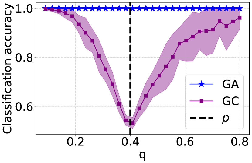
(a) Positive result, part 1 Theorem 2

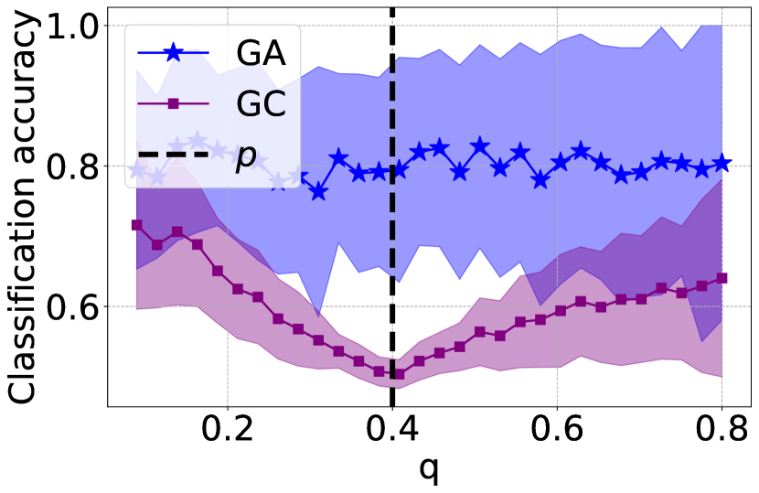
(b) Negative result, part 2 Theorem 2

Figure 1: Demonstration of part 1 and 2 of Theorem 2.

Varying the distance of the means of the node features. We illustrate how the attention coefficients and the accuracy change with the distance $\|\mu\|$. We fix $p=0.4$ and $q=0.33$ (this makes the graphs sufficiently noisy). We vary $\|\mu\|$ from $0.1\sigma\sqrt{\log n/(n\max(p,q))}$ to $20\sigma\sqrt{\log n}$. Fig. 2(a) illustrates Proposition 1. We observe empirically the separation of intra- and inter-$\gamma$ as claimed in Proposition 1. Fig. 2(b) illustrates a combination of parts 1 and 2 of Theorem 2. We observe that when the edge features are clean and $|p-q|$ is small then graph attention is better than graph convolution.

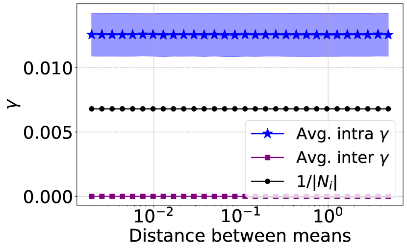
(a) Proposition 1

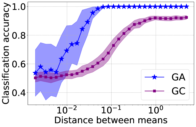
(b) Parts 1 and 2 of Theorem 2

Figure 2: This figure demonstrates how the attention coefficients and the accuracy are changing as a function of the distance between the means of the node features.

5.2 Noisy edge features

We set $\zeta=0.1$ and we pick the mean of the edge features $\nu$ such that $\|\nu\|\geq 100\zeta$.

Varying $q$. We fix $p=0.4$ and we vary $q$ from $\log^{2}/n$ to $2p$. We perform two experiments to demonstrate parts 1 and 2 of Theorem 4, For part 1, which is the positive result, we pick $\mu$ such that $\|\mu\|=8\sigma\frac{p+q}{|p-q|}\sqrt{\log n/(n\max(p,q))}$. For part 2, which is the negative result, we set $\|\mu\|=0.1\sigma\frac{p+q}{|p-q|}\sqrt{\log n/(n\max(p,q))}$. In Fig. 3(a) we present the positive result for graph attention and we also compare graph attention to graph convolution. We observe that for any value of $q$ graph attention has very similar performance to graph convolution. In Fig. 3(b) we present the negative result for graph attention. In this experiment, graph attention has very similar performance to graph convolution because the attention coefficients are approximately uniform.

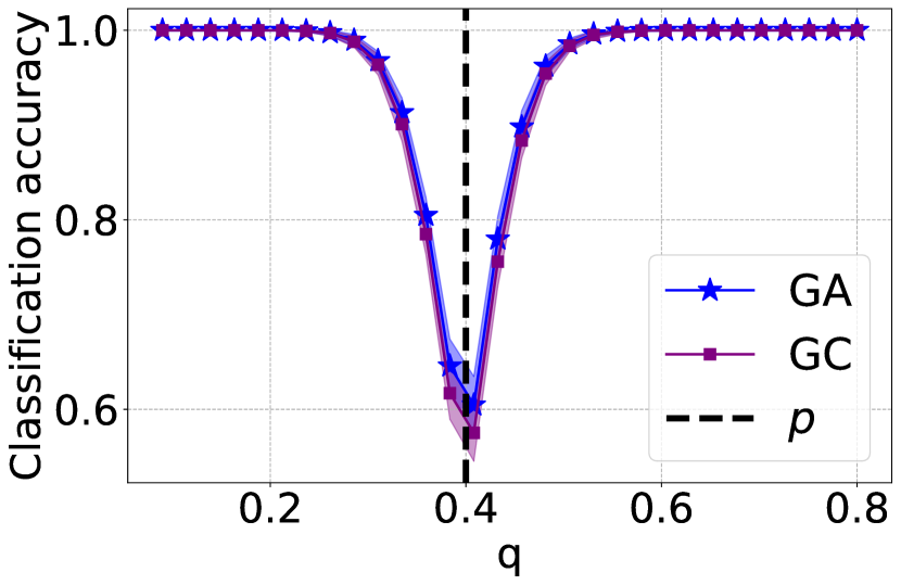
(a) Positive result, part 1 Theorem 4

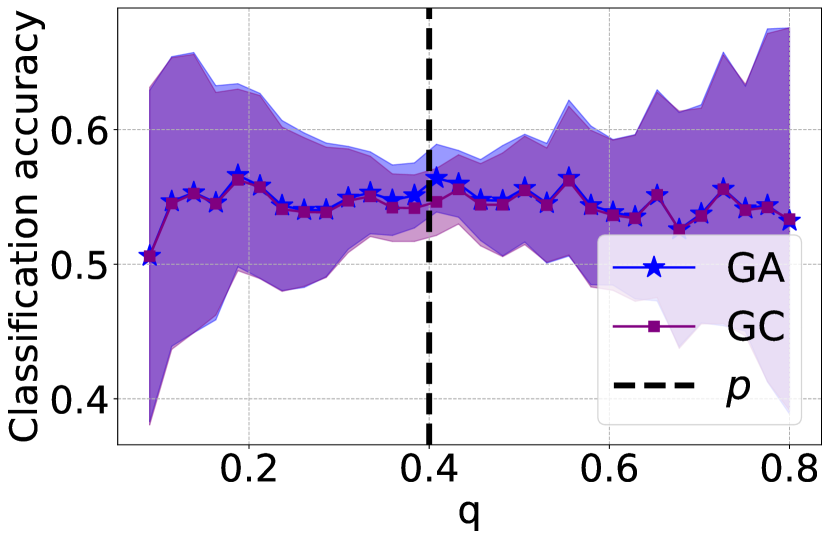
(b) Negative result, part 2 Theorem 4

Figure 3: Demonstration of part 1 and 2 of Theorem 4.

Varying the distance of the means of the node features. In this experiment we illustrate how the attention coefficients and the accuracy change as a function of the distance $\|\mu\|$. We fix $p=0.4$ and $q=0.33$ (this makes the graphs sufficiently noisy). We vary $\|\mu\|$ from $0.01\sigma\frac{p+q}{|p-q|}\sqrt{\log n/(n\max(p,q))}$ to $20\sigma\sqrt{\log n}$. Fig. 4(a) illustrates Proposition 3. We observe empirically that intra- and inter-$\gamma$ concentrate around the same value and they are both approximately uniform as claimed in Proposition 3. Fig. 4(b) illustrates a combination of parts 1 and 2 of Theorem 4. We observe that graph attention has very similar performance to graph convolution.

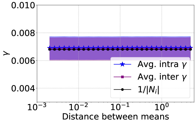
(a) Proposition 3

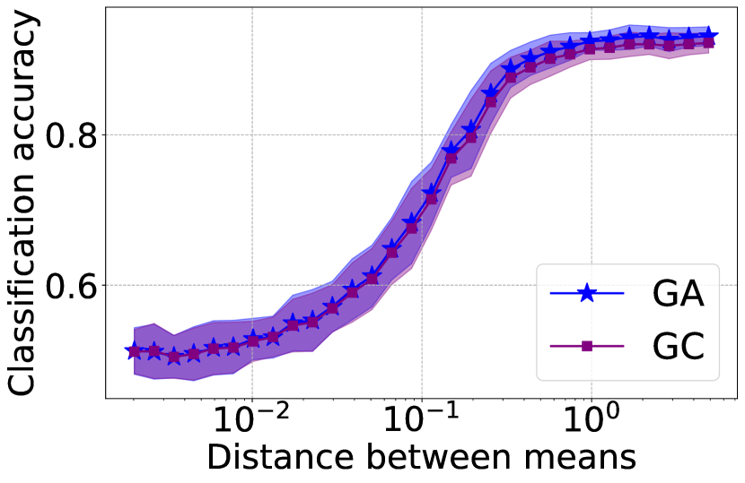
(b) Parts 1 and 2 of Theorem 4

Figure 4: This figure demonstrates how the attention coefficients and the accuracy are changing as a function of the distance between the means of the node features.

Attention coefficients for varying the distance of the means of the edge features. In this experiment we demonstrate how the attention coefficients scale as a function of the distance between the means of the edge features. This is basically a combination of the results in Proposition 1 and Proposition 3. We fix $p=0.4$ and $q=0.33$ (this makes the graphs sufficiently noisy). We vary $\|\nu\|$ from $0.01\zeta\sqrt{\log(0.5n^{2}(p+q))}$ to $30\zeta\sqrt{\log(0.5n^{2}(p+q))}$. The results are presented in Fig. 5. We observe that for small distance between the means of the edge features the attention coefficients concentrate around the uniform measure, see Proposition 3, while as the distance increases then the intra-$\gamma$ increase up to the value $2/np$, see Proposition 1 and the inter-$\gamma$ become very small, see Proposition 1.

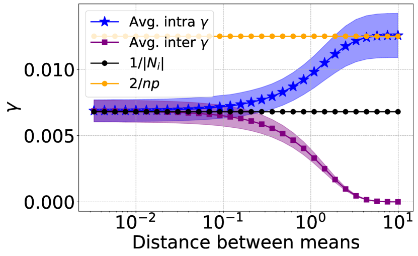
Figure 5: Proposition 1 and Proposition 3.

6 Experiments on Real Data

We use the popular real data Amazon Computers, Amazon Photos, Cora, PubMed, and CiteSeer. These data are publicly available and can be downloaded from [15]. The datasets come with multiple classes, however, for each of our experiments we do a one-v.s.-all classification. This is a semi-supervised problem, only a fraction of the training nodes have labels. The rest of the nodes are used for measuring prediction accuracy. For Cora, PubMed and CiteSeer we use the train/test split that is given by [15]. For Amazon Computers and Photos where the train/test split is not given we sample randomly $1\%$ of the nodes for training, the rest are used for testing. For each dataset we split the number of features into the first half and second half. The former is used for node features and the latter is used for edge features. The edge features are given by the concatenation of the features adjacent to the edge. We present results averaged over $5$ trials to account for randomness in initialization of parameters.

We observe that graph attention is giving similar attention mass to intra- and inter-edges as graph convolution which uses uniform weights as attention coefficients. This also explains the that there is no clear winner between graph attention and graph convolution when it comes to performance. In Table 1 we illustrate these observations. We present results for class $0$ and $1$ of each dataset. The experiments for the other classes are shown in the appendix. In Table 1 the intra-mass column is the percentage of the total probability mass assigned to intra-edges by intra-edge attention coefficients. Similarly for the inter-mass column. We observe that graph attention and graph convolution assign similar percentage of the mass to intra- and inter-edges. This results in graph attention performing similarly to graph convolution. We observe the same results for the rest of the classes in the appendix. It is important to mention that the attention coefficients of graph attention might not be exactly uniform or up to a constant uniform since our assumptions for CSBM might be violated, however, we still observe that graph attention has overall the same allocation of intra- and inter-mass to graph convolution. Finally, we observe that the majority of mass is assigned to intra-edges. This is expected since we are solving one-v.s.-all classification problems. However, we would still expect graph attention to have much better mass allocation for inter-edges than graph convolution, but it does not.

Table 1: Percentages of intra- and inter-mass allocation for graph attention (GA) and graph convolution (GC), and test accuracy.

data	class	method	intra-m	inter-m	acc.
Amzn Co.	$0$	GC	$98.7$	$1.3$	$96.8$
		GA	$98.1$	$1.9$	$96.7$
	$1$	GC	$93.6$	$6.4$	$91.4$
		GA	$93.3$	$6.7$	$88.7$
Amzn Ph.	$0$	GC	$99.0$	$1.0$	$95.1$
		GA	$98.8$	$1.2$	$96.0$
	$1$	GC	$94.9$	$5.1$	$94.2$
		GA	$95.5$	$4.5$	$89.0$
Cora	$0$	GC	$94.2$	$5.8$	$89.5$
		GA	$94.7$	$5.3$	$88.6$
	$1$	GC	$97.3$	$2.7$	$92.3$
		GA	$97.4$	$2.6$	$93.7$
PubMed	$0$	GC	$92.2$	$7.8$	$82.1$
		GA	$92.1$	$7.9$	$82.8$
	$1$	GC	$91.4$	$8.6$	$58.8$
		GA	$90.6$	$9.4$	$59.5$
CiteSeer	$0$	GC	$94.3$	$5.7$	$92.0$
		GA	$94.4$	$5.6$	$91.6$
	$1$	GC	$92.6$	$7.4$	$82.6$
		GA	$92.8$	$7.2$	$82.8$

7 Conclusion

We study conditions on the parameter of the CSBM with edge features such that graph attention can achieve or fail perfect node classification. We split our results into two parts. The first part is when the edge features are clean and the second part is when the edge features are noisy. If the edge features are clean we show that graph attention is able to distinguish intra from inter attention coefficients which allows us to prove that the condition for perfect classification is better than that of graph convolution. If the edge features are noisy we show that the majority of attention coefficients are up to a constant uniform which then implies that graph attention performs similarly to graph convolution.

Working with synthetic data models has a lot of limitations due to their gap with real data, but they also have very important advantages such as providing a solid insight about the performance of methods. It is more productive to discuss limitations in our analysis for potential future researchers who might wish to extend the present work. A limitation of our analysis is the assumption of a fixed $w$ for our negative results. It would be interesting future work to set $w$ to be the optimal solution of some expected loss function. Finally, it would be interesting to study the performance of methods beyond perfect classification.

Appendix A Elementary results

Since $(\epsilon_{i})_{i\in[n]}\sim\mbox{Ber}(\frac{1}{2})$, by the Chernoff bound [33, Section 2] we have that the number of nodes in each class satisfies

$$P\left(\frac{|C_{0}|}{n},\frac{|C_{1}|}{n}\in\left[\frac{1}{2}-o_{n}(1),\frac{1}{2}+o_{n}(1)\right]\right)\geq 1-1/\mathrm{poly}(n).$$

Proposition 1 (Concentration of degrees, [5]).

Assume that the graph density is $p,q=\Omega\left(\frac{\log^{2}n}{n}\right)$. Then for any constant $c>0$, with probability at least $1-2n^{-c}$, we have for all $i\in[n]$ that

$$|N_{i}| =\frac{n}{2}(p+q)(1\pm o_{n}(1))$$

where the error term $o_{n}(1)=O\left({\sqrt{\frac{c}{\log n}}}\right)$.

Proof.

Note that $|N_{i}|$ is a sum of $n$ Bernoulli random variables, hence, we have by the Chernoff bound [33, Section 2] that

$$P\left(|N_{i}|\in\left[\frac{n}{2}(p+q)(1-\delta),\frac{n}{2}(p+q)(1+\delta)\right]^{c}\right)\leq 2\exp(-Cn(p+q)\delta^{2}),$$

for some $C>0$. We now choose $\delta=\sqrt{\frac{(c+1)\log n}{Cn(p+q)}}$ for a large constant $c>0$. Note that since $p,q=\Omega\left(\frac{\log^{2}n}{n}\right)$, we have that $\delta=O\left(\sqrt{\frac{c}{\log n}}\right)=o_{n}(1)$. Then following a union bound over $i\in[n]$, we obtain that with probability at least $1-2n^{-c}$,

$$|N_{i}|=\frac{n}{2}(p+q)\left(1\pm O\Big{(}\sqrt{\frac{c}{\log n}}\Big{)}\right)\;\text{for all }i\in[n]$$

∎

Proposition 2 (Concentration of number of neighbors in each class).

Assume that the graph density is $p,q=\Omega\left(\frac{\log^{2}n}{n}\right)$. Then for any constant $c>0$, with probability at least $1-2n^{-c}$,

$$|N_{i}\cap C_{l}| =\frac{n}{2}p(1\pm o_{n}(1))\quad\text{for all }i\in C_{l}\mbox{ and }l\in\{0,1\}$$

$$|N_{i}\cap C_{l}| =\frac{n}{2}q(1\pm o_{n}(1))\quad\text{for all }i\in C_{l}^{c}\mbox{ and }l\in\{0,1\}$$

where the error term $o_{n}(1)=O\left({\sqrt{\frac{c}{\log n}}}\right)$.

Proof.

For any two distinct nodes $i,j\in[n]$ we have that $|N_{i}\cap C_{l}|=\sum_{j\in C_{l}}a_{ij}$. This is a sum of independent Bernoulli random variables, with mean $\mathbb{E}|N_{i}\cap C_{l}|=\frac{n}{2}p$ if $i\in C_{l}$ and $\mathbb{E}|N_{i}\cap C_{l}|=\frac{n}{2}q$ if $i\in C_{l}^{c}$. Denote $\mu_{ij}=\mathbb{E}|N_{i}\cap C_{l}|$. Therefore, by the Chernoff bound [33, Section 2], we have for a fixed pair of nodes $(i,j)$ that

$$P\left(|N_{i}\cap C_{l}|\in\left(\mu_{ij}(1-\delta_{ij}),\mu_{ij}(1+\delta_{ij})\right)^{c}\right)\leq 2\exp(-C\mu_{ij}\delta_{ij}^{2})$$

for some constant $C>0$. We now choose $\delta_{ij}=\sqrt{\frac{(c+2)\log n}{C\mu_{ij}}}$ for any large $c>0$. Note that since $p,q=\Omega\left(\frac{\log^{2}n}{n}\right)$, we have that $\delta_{ij}=O\left(\sqrt{\frac{c}{\log n}}\right)=o_{n}(1)$. Then following a union bound over all nodes $i\in[n]$, we obtain that with probability at least $1-2n^{-c}$, for all pairs of nodes $(i,j)$ we have

$$|N_{i}\cap C_{l}| =\frac{n}{2}p(1\pm o_{n}(1))\quad\text{for all }i\in C_{l}\mbox{ and }l\in\{0,1\}$$

$$|N_{i}\cap C_{l}| =\frac{n}{2}q(1\pm o_{n}(1))\quad\text{for all }i\in C_{l}^{c}\mbox{ and }l\in\{0,1\}.$$

∎

Proposition 3 (Concentration of uncommon neighbors).

Assume that the graph density parameters satisfy $\max\{p,q\}\leq 1-36\log n/n$, then with probability at least $1-n^{-1}$ we have that for all $i,j\in[n]$, $i\neq j$,

1. If $i,j\in C_{l}$ and $l\in\{0,1\}$, then

   $$|(N_{i}\cup N_{j})\backslash(N_{i}\cap N_{j})|\geq\frac{n}{2}(p+q-p^{2}-q^{2})(1-o_{n}(1)),$$

   moreover,

   $$|((N_{i}\cup N_{j})\backslash(N_{i}\cap N_{j}))\cap C_{l}| \geq\frac{n}{2}(p-p^{2})(1-o_{n}(1)),$$

   $$|((N_{i}\cup N_{j})\backslash(N_{i}\cap N_{j}))\cap C_{l}^{c}| \geq\frac{n}{2}(q-q^{2})(1-o_{n}(1)).$$

2. If $i\in C_{l}$, $j\in C_{l}^{c}$ and $l\in\{0,1\}$, then

   $$|(N_{i}\cup N_{j})\backslash(N_{i}\cap N_{j})|\geq\frac{n}{2}(p+q-2pq)(1-o_{n}(1)).$$

Proof.

Consider an arbitrary pair of nodes $i,j\in C_{0}$ such that $i\neq j$. The probability that a node $l\in[n]$ is a neighbor of exactly one of $i,j$ is $2p(1-p)$ if $l\in C_{0}$ and $2q(1-q)$ if $l\in C_{1}$. Let $J_{ij}:=(N_{i}\cup N_{j})\backslash(N_{i}\cap N_{j})$. Then $J_{ij}$ is a sum of independent Bernoulli random variables and $\mathbb{E}|J_{ij}|=n(p(1-p)+q(1-q))$. Hence, by the multiplicative Chernoff bound we have that for any $0<\delta\leq 1$,

$$P\Big{(}|J_{ij}|\leq\mathbb{E}|J_{ij}|(1-\delta)\Big{)}\leq\exp\left(-\frac{1}{3}\delta^{2}\mathbb{E}|J_{ij}|\right).$$

In what follows we find a suitable choice for $\delta$. Because $\max\{p,q\}\leq 1-36\log n/n$, we have that

$$p+q-p^{2}-q^{2}\geq\max\{p-p^{2},q-q^{2}\}\geq 1-\frac{36\log n}{n}-\left(1-\frac{36\log n}{n}\right)^{2}=\frac{36\log n}{n}\left(1-\frac{36\log n}{n}\right)$$

and hence

$$3\sqrt{\frac{\log n}{\mathbb{E}|J_{ij}|}}=3\sqrt{\frac{\log n}{n(p+q-p^{2}-q^{2})}}\leq\frac{1}{2\sqrt{1-\frac{36\log n}{n}}}\leq\frac{1}{2}\left(\frac{1}{1-6\sqrt{\frac{\log n}{n}}}\right)\leq\frac{1}{2}\left(1+O\left(\sqrt{\frac{\log n}{n}}\right)\right).$$

Therefore we may choose $\delta=3\sqrt{\log n}/\sqrt{\mathbb{E}|J_{ij}|}$ and apply the union bound over all $i,j\in[n]$ to get that with probability at least $1-n^{-1}$, for all $i,j\in C_{0}$, $i\neq j$,

$$|J_{ij}|\geq\mathbb{E}|J_{ij}|(1-\delta)=n(p+q-p^{2}-q^{2})\left(1-\frac{1}{2}-O\left(\sqrt{\frac{\log n}{n}}\right)\right)=\frac{n}{2}(p+q-p^{2}-q^{2})(1-o_{n}(1)),$$

which proves the claim on the cardinality of $|(N_{i}\cup N_{j})\backslash(N_{i}\cap N_{j})|$ for $i,j\in C_{l}$ and $l=0$. The other cases follow analogously. ∎

Appendix B Proofs for clean edge features

Without loss of generality we ignore the self-loops in the graph. This is because adding self-loops only introduces an additional independent random variable, which changes the results up to an unimportant constant. Moreover, for proofs that rely on constructing the function $\Psi$ we provide the general definition for any $p,q$. However, since the proofs for $p>q$ and $q>p$ are almost identical, we provide the proofs for the case $p>q$. The proof for $q>p$ is different up to flipping signs and considering the fact that on expectation the inter-edges are more than the intra-edges.

Proposition 1.

Let $(A,X,E)\sim CSBM(n,p,q,\mu,\nu,\sigma,\zeta)$, and assume that $\|\nu\|\geq\omega(\zeta\sqrt{\log(|\mathcal{E}|)})$. If $p>q$, we have that

$$\gamma_{ij}=\begin{cases}\frac{2}{np}(1\pm o_{n}(1))&i,j\in C_{0}\mbox{ or }i,j\in C_{1}\\ o\left(\frac{1}{n(p+q)}\right)&\mbox{otherwise.}\\ \end{cases}$$

with probability $1-o_{n}(1)$. If $q>p$, we have that

$$\gamma_{ij}=\begin{cases}o\left(\frac{1}{n(p+q)}\right)&i,j\in C_{0}\mbox{ or }i,j\in C_{1}\\ \frac{2}{nq}(1\pm o_{n}(1))&\mbox{otherwise.}\\ \end{cases}$$

with probability $1-o_{n}(1)$.

Proof.

We will construct a $\Psi$ function such that with high probability it is able to separate intra- from inter-edges and it concentrates around its mean. Then we will use $\Psi$ to show that the attention coefficients $\gamma_{ij}$ concentrate as well. Define $s:=\operatorname{sign}(p-q)\nu/(\zeta\|\nu\|)$ and $\Psi(E_{(i,j)}):=\alpha s^{T}E_{(i,j)}$ where $\alpha>0$ is a scaling parameter whose value we will determine later. We will prove the result for the case that $p>q$, the result for $q>p$ is similar. We will show that function $\Psi$ concentrates around its mean. First, let us rewrite $E_{(i,j)}:=(2\epsilon_{i}-1)(2\epsilon_{j}-1)\nu+\zeta f_{(i,j)}$. Thus we have that $\Psi(E_{(i,j)})=\alpha(2\epsilon_{i}-1)(2\epsilon_{j}-1)\|\nu\|/\zeta+\alpha\tilde{f}_{(i,j)}$ where $f_{(i,j)}:=\zeta s^{T}f_{(i,j)}$. Because $\|\zeta s\|=1$ we know that $\tilde{f}_{(i,j)}\sim N(0,1)$, and thus using upper bound on the Gaussian tail probability, e.g. see [33, Section 2], we have that

$$P\left(|\tilde{f}_{(i,j)}|\geq 10c\sqrt{\log(|\mathcal{E}|)}\right)\leq\exp(100\log(|\mathcal{E}|)),$$

for some absolute constant $c>0$. Taking a union bound over all $(i,j)\in\mathcal{E}$ we have that

$$P\left(|\tilde{f}_{(i,j)}|<10\sqrt{\log(|\mathcal{E}|)}\ \forall(i,j)\in\mathcal{E}\right)\geq|\mathcal{E}|\exp(100\log(|\mathcal{E}|))=\frac{1}{|\mathcal{E}|^{99}}=o_{|\mathcal{E}|}(1)$$

Let $E^{*}$ denote that event that $|\tilde{f}_{(i,j)}|<10c\sqrt{\log(|\mathcal{E}|)}$ for all $(i,j)\in\mathcal{E}$. Then the above inequality says that the event $E^{*}$ happens with probability at least $1-o_{|\mathcal{E}|}(1)$. Let us assume that $E^{*}$ happens. Then we have that

$$\Psi(E_{(i,j)})=\begin{cases}\alpha\|\nu\|/\zeta\pm O(\alpha\sqrt{\log(|\mathcal{E}|)})&i,j\in C_{0}\mbox{ or }i,j\in C_{1}\\ -\alpha\|\nu\|/\zeta\pm O(\alpha\sqrt{\log(|\mathcal{E}|)})&\text{otherwise.}\end{cases}$$

If $i,j\in C_{0}$, then plugging in $\Psi$ into the attention coefficients $\gamma_{ij}$ we get that

$$\gamma_{ij} =\frac{\exp\left(\alpha\|\nu\|/\zeta\pm O(\alpha\sqrt{\log(|\mathcal{E}|)})\right)}{\sum_{\ell\in N_{i}\cap C_{0}}\exp\left(\alpha\|\nu\|/\zeta\pm O(\alpha\sqrt{\log(|\mathcal{E}|)})\right)+\sum_{\ell\in N_{i}\cap C_{1}}\exp\left(-\alpha\|\nu\|/\zeta\pm O(\alpha\sqrt{\log(|\mathcal{E}|)})\right)}$$

$$=\frac{1}{\sum_{\ell\in N_{i}\cap C_{0}}\exp\left(\pm O(\alpha\sqrt{\log(|\mathcal{E}|)})\right)+\sum_{\ell\in N_{i}\cap C_{1}}\exp\left(-2\alpha\|\nu\|/\zeta\pm O(\alpha\sqrt{\log(|\mathcal{E}|)})\right)}.$$

Note that because $\|\nu\|/\zeta=\omega(\sqrt{\log(|\mathcal{E}|)})$ we can set $\alpha$ such that $\alpha\sqrt{\log(|\mathcal{E}|)}=o_{n}(1)$ and $\alpha\|\nu\|/\zeta=\omega_{n}(1)$. Therefore we get

$$\gamma_{ij} =\frac{1}{\sum_{\ell\in N_{i}\cap C_{0}}\exp(\pm o_{n}(1))+\sum_{\ell\in N_{i}\cap C_{1}}\exp(-\omega_{n}(1))}=\frac{1}{|N_{i}\cap C_{0}|(1\pm o_{n}(1))+|N_{i}\cap C_{1}|o_{n}(1)}$$

$$=\frac{1}{|N_{i}\cap C_{0}|}(1\pm o_{n}(1))=\frac{2}{np}(1\pm o_{n}(1))$$

where the last equality follows from Proposition 2.

Following a similar reasoning for the other edges we get that when the event $E^{*}$ happens,

$$\gamma_{ij}=\begin{cases}\frac{2}{np}(1\pm o_{n}(1))&i,j\in C_{0}\mbox{ or }i,j\in C_{1}\\ o\left(\frac{1}{n(p+q)}\right)&\mbox{otherwise.}\\ \end{cases}$$

Noting that the event happens with probability at least $1-o_{n}(1)$ completes the proof. ∎

Theorem 2.

Let $(A,X,E)\sim CSBM(n,p,q,\mu,\nu,\sigma,\zeta)$, and assume that $\|\nu\|\geq\omega(\zeta\sqrt{\log(|\mathcal{E}|)})$.

1. If $\|\mu\|\geq\omega\left(\sigma\sqrt{\frac{\log{n}}{n\max(p,q)}}\right)$, then we can construct a graph attention architecture that classifies the nodes perfectly with probability $1-o_{n}(1)$.

2. If $\|\mu\|\leq K\sigma\sqrt{\frac{\log{n}}{n\max(p,q)}\left(1-\max(p,q)\right)}$ for some constant $K$, then for any fixed $\|w\|=1$ graph attention fails to perfectly classify the nodes with probability

   $$1-2\exp(-c^{\prime}(1-\max(p,q))\log n)$$

   for some constant $c^{\prime}$.

Proof.

We start by proving part 1 of the theorem. Define $w:=\operatorname{sign}(p-q)\mu/\|\mu\|$. We will prove the result for $p>q$ since the analysis for $q>p$ is similar. Write $x_{i}=(2\epsilon_{i}-1)\mu+\sigma g_{i}$ where $g_{i}\sim N(0,I)$. Denote $\tilde{g}_{j}:=w^{T}g_{j}$ for $j\in[n]$. Because $\|w\|=1$ we have $\tilde{g}_{j}\sim N(0,1)$. We will use the attention coefficients from Proposition 1 in the graph attention. Let $i\in C_{0}$. We have that

$$\hat{x}_{i} =\sum_{j\in[n]}\tilde{A}_{ij}\gamma_{ij}w^{T}x_{j}$$

$$=-\sum_{j\in N_{i}\cap C_{0}}\frac{2}{np}\|\mu\|(1\pm o_{n}(1))+\sum_{j\in N_{i}\cap C_{1}}o\left(\frac{1}{n(p+q)}\right)\|\mu\|$$

$$\ \ \ +\sigma\sum_{j\in N_{i}\cap C_{0}}\frac{2}{np}\tilde{g}_{j}(1\pm o_{n}(1))+\sigma\sum_{j\in N_{i}\cap C_{1}}o\left(\frac{1}{n(p+q)}\right)\tilde{g}_{j}$$

Let us first work with the sums for $\|\mu\|$. Using Proposition 2 we have that

$$\sum_{j\in N_{i}\cap C_{0}}\frac{2}{np}\|\mu\|(1\pm o_{n}(1))=\|\mu\|(1\pm o_{n}(1))$$

and

$$\sum_{j\in N_{i}\cap C_{1}}o\left(\frac{1}{n(p+q)}\right)\|\mu\|=\|\mu\|o_{n}(1)(1\pm o_{n}(1))$$

Putting the two sums for $\|\mu\|$ together we have that

$$-\sum_{j\in N_{i}\cap C_{0}}\frac{2}{np}\|\mu\|(1\pm o_{n}(1))+\sum_{j\in N_{i}\cap C_{1}}o\left(\frac{1}{n(p+q)}\right)\|\mu\|=-\|\mu\|(1\pm o_{n}(1)).$$

Let us now work with the sum of noise over $N_{i}\cap C_{0}$. This is a sum of $|N_{i}\cap C_{0}|$ standard normals. From Theorem 2.6.3. (General Hoeffding’s inequality) and from concentration of $|N_{i}\cap C_{0}|$ from Proposition 2 we have that

$$P\left(\left|\sum_{j\in N_{i}\cap C_{0}}\Theta\left(\frac{1}{np}\right)\tilde{g}_{j}\right|\geq\sqrt{\frac{10C^{2}\log{n}}{n\max(p,q)c}}\right)\leq 2\exp\left(-10\log{n}\right),$$

where $c$ is a constant, and $C$ is the sub-Gaussian constant for $\tilde{g}_{j}$. Taking a union bound over all $i\in C_{0}$, we have that with probability $1-o_{n}(1)$ we have that

$$\left|\sum_{j\in N_{i}\cap C_{0}}\Theta\left(\frac{1}{np}\right)\tilde{g}_{j}\right|<\sqrt{\frac{10C^{2}\log{n}}{n\max(p,q)c}},\ \forall i\in C_{0}.$$

Using similar concentration arguments we get that the second sum of the noise over $N_{i}\cap C_{1}$ is a smaller order term. Thus, since $\|\mu\|\geq\omega\left(\sigma\sqrt{\frac{\log{n}}{n\max(p,q)}}\right)$ we get

$$\hat{x}_{i}=-\|\mu\|(1\pm o_{n}(1))+o(\|\mu\|).$$

with probability $1-o_{n}(1)$. Therefore, with high probability nodes in $C_{0}$ are correctly classified. Using the same procedure for nodes in $C_{1}$ we get that these nodes are also classified correctly.

Let us now proceed with the proof of part 2. We will prove the result for $p>q$, the proof for the $q>p$ is similar. We will prove that the probability of classifying all nodes correctly is very small. Let us start with the event of correct classification of all nodes. Let $w$ be any vector satisfying $\|w\|=1$. Using the same sub-Gaussian concentration arguments as before and Proposition 1 we get that with probability $1-o_{n}(1)$ the event for perfect classification is

$$-w^{T}\mu(1\pm o_{n}(1))+\max_{i\in C_{0}}\sigma\sum_{j\in N_{i}}\gamma_{ij}w^{T}g_{j}<0$$

$$w^{T}\mu(1\pm o_{n}(1))+\min_{i\in C_{1}}\sigma\sum_{j\in N_{i}}\gamma_{ij}w^{T}g_{j}>0,$$

for nodes in $C_{0}$ and $C_{1}$, respectively. Let’s bound the probability of correct classification for $C_{0}$, the result for $C_{1}$ is similar.

$$P\left(-w^{T}\mu(1\pm o_{n}(1))+\max_{i\in C_{0}}\sigma\sum_{j\in N_{i}}\gamma_{ij}w^{T}g_{j}<0\right)$$

$$\leq P\left(\max_{i\in C_{0}}\sigma\sum_{j\in N_{i}}\gamma_{ij}w^{T}g_{j}<\|\mu\|(1\pm o_{n}(1))\right) \|w\|=1$$ using Cauchy-Schwartz and

$$\leq P\left(\max_{i\in C_{0}}\sum_{j\in N_{i}}\gamma_{ij}w^{T}g_{j}<K\sqrt{\frac{\log{n}}{n\max(p,q)}(1-\max(p,q))}\right)$$

$$=P\left(\max_{i\in C_{0}}\sum_{j\in N_{i}}\gamma_{ij}w^{T}g_{j}<K\sqrt{\frac{\log{n}}{np}\left(1-p\right)}\right)$$

The remaining of the proof is similar to the proof in [5]. We will utilize Sudakov’s minoration inequality [33, Section 7.4] to obtain a lower bound on the expected supremum of the corresponding Gaussian process, and then use Borell’s inequality [2, Section 2.1] to upper bound the probability.

Let $Z_{i}:=\sum_{j\in N_{i}}\gamma_{ij}w^{T}g_{j}$ for $i\in C_{0}$. To apply Sudakov’s minoration result, we also define the canonical metric $d_{T}(i,j)=\sqrt{\mathbb{E}[(Z_{i}-Z_{j})^{2}]}$ for any $i,j\in C_{0}$. In what follows we will first compute $\mathbb{E}[(Z_{i}-Z_{j})^{2}]$ and then the metric. Conditioned on the events described by Proposition 1, Proposition 2 and Proposition 3, we know that with probability at least $1-o_{n}(1)$,

$$\mathbb{E}[(Z_{i}-Z_{j})^{2}] =\mathbb{E}\left[\left(\sum_{l\in N_{i}}\gamma_{il}w^{T}g_{l}\right)^{2}+\left(\sum_{k\in N_{j}}\gamma_{jk}w^{T}g_{k}\right)^{2}-2\left(\sum_{l\in N_{i}}\gamma_{il}w^{T}g_{l}\right)\left(\sum_{k\in N_{j}}\gamma_{jk}w^{T}g_{k}\right)\right]$$

$$=\sum_{l\in N_{i}}\gamma_{il}^{2}+\sum_{l\in N_{j}}\gamma_{jl}^{2}-2\sum_{l\in N_{i}\cap N_{j}}\gamma_{il}\gamma_{jl}$$

$$\geq\sum_{l\in(N_{i}\backslash(N_{i}\cap N_{j}))\cap C_{0}}\gamma_{il}^{2}+\sum_{l\in(N_{j}\backslash(N_{i}\cap N_{j}))\cap C_{0}}\gamma_{jl}^{2}$$

$$=\sum_{l\in((N_{i}\cup N_{j})\backslash(N_{i}\cap N_{j}))\cap C_{0}}\frac{4}{n^{2}p^{2}}(1\pm o_{n}(1))$$

$$=\frac{n}{2}(p-p^{2})(1-o_{n}(1))\cdot\frac{4}{n^{2}p^{2}}(1\pm o_{n}(1))$$

$$=\frac{2}{np}(1-p)(1-o_{n}(1)).$$

Thus

$$d_{T}(i,j)\geq\sqrt{\frac{2}{np}}\sqrt{1-p}(1-o_{n}(1))$$

Using this result in Sudakov’s minoration inequality, we obtain that

$$\mathbb{E}[\max_{i}Z_{i}]\geq c\sqrt{\frac{\log n}{np}(1-p)}.$$

for some absolute constant $c$. We now use Borell’s inequality [2, Section 2.1] and the fact that the variance of the Gaussian data after graph attention convolution is $\Theta(1/np)$ to obtain that for any $t>0$,

$$P\left(\max_{i\in C_{0}}Z_{i}\leq\mathbb{E}\max_{i\in C_{0}}Z_{i}-t\right)\leq 2\exp(-Ct^{2}np)$$

$$\implies\quad P\left(\max_{i\in C_{0}}Z_{i}\leq c\sqrt{\frac{\log n}{np}(1-p)}-t\right)\leq 2\exp(-Ct^{2}np)$$

for some absolute constant $C>0$. Now, for some small enough constant $K$ we may set $t$ such that

$$t=c\sqrt{\frac{\log n}{np}(1-p)}-K\sqrt{\frac{\log{n}}{np}(1-p)}=\Omega\left(\sqrt{\frac{\log n}{np}(1-p)}\right).$$

Plugging this $t$ in the above probability we have that for some constant $c^{\prime}>0$,

$$P\left(\max_{i\in C_{0}}Z_{i}\leq K\sqrt{\frac{\log{n}}{np}(1-p)}\right)\leq 2\exp(-c^{\prime}(1-p)\log n).$$

∎

Appendix C Proofs for noisy edge features

For noisy edge features we have $\|\nu\|\leq K\zeta$ for some $K=\mathcal{O}(1)$. We may write $E_{(i,j)}=(2\epsilon_{i}-1)(2\epsilon_{j}-1)\nu+\zeta f_{(i,j)}$ where $f_{(i,j)}\sim N(0,I)$. That is, $E_{(i,j)}=\nu+\zeta f_{(i,j)}$ if $(i,j)$ is an intra-edge and $E_{(i,j)}=-\nu+\zeta f_{(i,j)}$ if $(i,j)$ is an inter-edge. Recall that in this work we consider attention architecture $\Psi$ that is a composition of a Lipschitz function and a linear function. That is, for $(i,j)\in\mathcal{E}$ the attention coefficient is given as

$$\gamma_{ij}=\frac{\exp(\Psi(E_{(i,j)}))}{\sum_{l\in N_{i}}\exp(\Psi(E_{(i,l)}))}=\frac{\exp(\phi((2\epsilon_{i}-1)(2\epsilon_{j}-1)s^{T}\nu+\zeta s^{T}f_{(i,j)}))}{\sum_{l\in N_{i}}\exp(\phi((2\epsilon_{i}-1)(2\epsilon_{l}-1)s^{T}\nu+\zeta s^{T}f_{(i,l)}))}$$

where $\phi:\mathbb{R}\rightarrow\mathbb{R}$ is Lipschitz continuous with Lipschitz constant $L$ and $|\phi(0)|\leq R$ for some $R\geq 0$. Naturally, both $L$ and $R$ do not depend on $n$. The linear function has learnable parameters $s$. We assume that $\|s\|$ is bounded. Therefore, in subsequent analysis we also assume $\|s\|=1$. This assumption is without loss of generality, because as long as $s$ is bounded and nonzero, one may always write $s=rs^{\prime}$ for some $\|s^{\prime}\|=1$ and absolute constant $r>0$. The additional constant $r$ does affect the computations we need for the proofs.

We start by defining a number of index sets which we will use extensively in the proofs. First let us define a subset of nodes whose incident edge features are “nice”,

$$\mathcal{A}:=\{i\in[n]:|s^{T}f_{(i,j)}|\leq 10\sqrt{\log(n(p+q))}\ \forall j\in N_{i}\}$$ (1)

In addition, for $i\in[n]$ define the following sets

$$J_{i,0} :=\left\{j\in N_{i}\cap C_{0}:|s^{T}f_{(i,j)}|\leq\sqrt{10}\right\},$$

$$J_{i,1} :=\left\{j\in N_{i}\cap C_{1}:|s^{T}f_{(i,j)}|\leq\sqrt{10}\right\},$$

$$B_{i,0}^{t} :=\left\{j\in N_{i}\cap C_{0}:2^{t-1}\leq|s^{T}f_{(i,j)}|\leq 2^{t}\right\},t=1,2,\ldots,T,$$

$$B_{i,1}^{t} :=\left\{j\in N_{i}\cap C_{1}:2^{t-1}\leq|s^{T}f_{(i,j)}|\leq 2^{t}\right\},t=1,2,\ldots,T$$

where $T=\left\lceil\log_{2}\left(10\sqrt{\log(n(p+q))}\right)\right\rceil$. Finally, for a pair of nodes $i,j\in[n]$ we define

$$\widehat{J}_{ij}:=\left\{l\in(N_{i}\cup N_{j})\backslash(N_{i}\cap N_{j}):|s^{T}f_{(i,j)}|\leq\sqrt{10}\right\}.$$

Since the sets defined above depends on the random variable $s^{T}f_{(i,j)}$, the cardinalities of the sets are also random variables. In the following we provide high probability bounds on the cardinalities of these sets.

Claim C.1 (Lower bound of $|\mathcal{A}|$).

With probability at least $1-o_{n}(1)$ we have $|\mathcal{A}|\geq n-O(n/\log n)$, and consequently $|\mathcal{A}\cap C_{0}|\geq|C_{0}|-O(n/\log n)$ and $|\mathcal{A}\cap C_{1}|\geq|C_{1}|-O(n/\log n)$.

Proof.

We start by providing an upper bound on the cardinality of the following set

$$\mathcal{A}_{E}:=\left\{(i,j)\in\mathcal{E}:|s^{T}f_{(i,j)}|\geq 10\sqrt{\log(n(p+q))}\right\}.$$

Note that we may write $|\mathcal{A}_{E}|$ as

$$|\mathcal{A}_{E}|=\sum_{(i,j)\in\mathcal{E}}\mathbf{1}_{\left\{|s^{T}f_{(i,j)}|\geq 10\sqrt{\log(n(p+q))}\right\}},$$

and thus by the multiplicative Chernoff bound we get that for any $\delta>0$,

$$P\Big{(}|\mathcal{A}_{E}|\geq|\mathcal{E}|b(1+\delta)\Big{)}\leq\exp\left(-\tfrac{\delta^{2}}{2+\delta}|\mathcal{E}|b\right),$$ (2)

where

$$b:=P\left(|s^{T}f_{(i,j)}|\geq 10\sqrt{\log(n(p+q))}\right).$$

Moreover, from standard upper bound on Gaussian tail probability we know that $b<e^{-50\log(n(p+q))}$. Let us set

$$\delta:=\frac{1}{bn^{1/2}|\mathcal{E}|^{1/2}(p+q)}.$$

Using Proposition 1 we know that with probability at least $1-o_{n}(1)$ one has $|\mathcal{E}|=\frac{n^{2}}{2}(p+q)(1\pm o_{n}(1))$, and hence it follows that,

$$\delta=\frac{\sqrt{2}(1\pm o_{n}(1))}{b(n(p+q))^{3/2}}\geq\frac{\sqrt{2}(1\pm o_{n}(1))}{(n(p+q))^{3/2}e^{-50\log(n(p+q))}}=\omega_{n}(1).$$

This means that

$$\frac{\delta^{2}}{2+\delta}|\mathcal{E}|b\geq\Omega(\delta|\mathcal{E}|b)=\Omega\left(\frac{|\mathcal{E}|b}{bn^{1/2}|\mathcal{E}|^{1/2}(p+q)}\right)=\Omega\left(\frac{|\mathcal{E}|^{1/2}}{n^{1/2}(p+q)}\right)=\Omega\left(\frac{n}{\sqrt{n(p+q)}}\right)\geq\Omega(\sqrt{n}).$$ (3)

On the other hand,

$$\begin{split}|\mathcal{E}|b(1+\delta)&=|\mathcal{E}|b+\frac{|\mathcal{E}|b}{bn^{1/2}|\mathcal{E}|^{1/2}(p+q)}\leq|\mathcal{E}|e^{-50\log(n(p+q))}+\frac{|\mathcal{E}|^{1/2}}{n^{1/2}(p+q)}\\ &\leq\frac{n^{2}}{2}(p+q)(1\pm o_{n}(1))\frac{1}{(n(p+q))^{50}}+\frac{n}{\sqrt{2n(p+q)}}(1\pm o_{n}(1))\\ &=O\left(\frac{n}{(n(p+q))^{49}}\right)+O\left(\frac{n}{\sqrt{n(p+q)}}\right)\leq O\left(\frac{n}{\log n}\right),\end{split}$$ (4)

where the last inequality follows from the assumption that $p,q=\Omega(\log^{2}n/n)$. Combining equation 2, equation 3 and equation 4, with probability at least $1-o_{n}(1)$ we have that

$$|\mathcal{A}_{E}|\leq O(n/\log n).$$

This means that for any subset $S\subseteq[n]$, e.g. we may take $S=[n]$, $S=C_{0}$ or $S=C_{1}$,

$$\left|\left\{i\in S:\exists j\in N_{i}\ \mbox{such that}\ |s^{T}f_{(i,j)}|\geq 10\sqrt{\log(n(p+q))}\right\}\right|\leq|\mathcal{A}_{E}|\leq O(n/\log n),$$

which proves the claim. ∎

Claim C.2 (Lower bounds of $|J_{i,0}|$ and $|J_{i,1}|$ [16]).

With probability at least $1-o_{n}(1)$, we have that for all $i\in[n]$,

$$|J_{i,0}|\geq\frac{9}{10}|N_{i}\cap C_{0}|\ \ \mbox{and}\ \ |J_{i,1}|\geq\frac{9}{10}|N_{i}\cap C_{1}|.$$

Proof.

We prove the result for $J_{i,0}$, the result for $J_{i,1}$ follows analogously. Consider an arbitrary $i\in[n]$. For each $j\in N_{i}\cap C_{0}$ we have

$$P(|s^{T}f_{(i,j)}|\geq\sqrt{10})\leq e^{-50},$$

which follows from upper bound of the Gaussian tail, e.g., see Proposition 2.1.2 in [33]. Denote $J_{i,0}^{c}:=(N_{i}\cap C_{0})\backslash J_{i,0}$. Then

$$\mathbb{E}\left[|J_{i,0}^{c}|\right]=\mathbb{E}\left[\sum_{j\in N_{i}\cap C_{0}}\mathbf{1}_{\left\{||s^{T}f_{(i,j)}|\geq\sqrt{10}|\right\}}\right]\leq e^{-50}|N_{i}\cap C_{0}|.$$

Apply Chernoff bound (see, e.g., Theorem 2.3.4 in [34]) we have

$$P\left(|J_{i,0}^{c}|\geq\frac{1}{10}|N_{i}\cap C_{0}|\right) \leq e^{-\mathbb{E}\left[|J_{i,0}^{c}|\right]}\left(\frac{e\mathbb{E}\left[|J_{i,0}^{c}|\right]}{|N_{i}\cap C_{0}|/10}\right)^{|N_{i}\cap C_{0}|/10}$$

$$\leq\left(\frac{ee^{-50}|N_{i}\cap C_{0}|}{|N_{i}\cap C_{0}|/10}\right)^{|N_{i}\cap C_{0}|/10}$$

$$=\exp\left(-\left(\frac{1}{2}-\frac{\log 10}{10}-\frac{1}{10}\right)|N_{i}\cap C_{0}|\right)$$

$$\leq\exp\left(-\frac{4}{25}|N_{i}\cap C_{0}|\right).$$

Apply the union bound we get

$$P\left(|J_{i,0}|\geq\frac{9}{10}|N_{i}\cap C_{0}|,\forall i\in[n]\right) \geq 1-\sum_{i\in[n]}\exp\left(-\frac{4}{25}|N_{i}\cap C_{0}|\right)$$

$$\geq(1-o_{n}(1))\left(1-n\exp\left(-\frac{4}{25}n\min\{p,q\}(1-o_{n}(1))\right)\right)$$

$$=1-o_{n}(1).$$

∎

Claim C.3 (Lower bound of $|\widehat{J}_{ij}|$).

Assume that the graph density parameters satisfy $\max\{p,q\}\leq 1-36\log n/n$, then with probability at least $1-o_{n}(1)$ we have that for all $i,j\in C_{l}$ and $l\in\{0,1\}$, $i\neq j$,

$$|\widehat{J}_{ij}\cap C_{l}| \geq\frac{9}{10}|((N_{i}\cup N_{j})\backslash(N_{i}\cap N_{j}))\cap C_{l}|,$$

$$|\widehat{J}_{ij}\cap C_{l}^{c}| \geq\frac{9}{10}|((N_{i}\cup N_{j})\backslash(N_{i}\cap N_{j}))\cap C_{l}^{c}|.$$

Proof.

We prove the result for $i,j\in C_{l}$ and $l=0$, the other cases follow analogously. Consider an arbitrary pair of nodes $i,j\in C_{0}$ and$i\neq j$. For each $k\in((N_{i}\cup N_{j})\backslash(N_{i}\cap N_{j}))\cap C_{0}$ we have

$$P(|s^{T}f_{(i,k)}|\geq\sqrt{10})\leq e^{-50}$$

as in the proof of Claim C.2. Moreover, by following the same reasoning as in the proof of Claim C.2, we get that

$$P\left(|\widehat{J}_{ij}\cap C_{0}|\geq\frac{9}{10}|((N_{i}\cup N_{j})\backslash(N_{i}\cap N_{j}))\cap C_{0}|,\forall i,j\in C_{0},i\neq j\right)$$

$$\geq~{} 1-\sum_{i,j\in C_{0},i\neq j}\exp\left(-\frac{4}{25}|((N_{i}\cup N_{j})\backslash(N_{i}\cap N_{j}))\cap C_{0}|\right)$$

$$\geq~{} (1-o_{n}(1))\left(1-n^{2}\exp\left(-\frac{4}{25}\frac{n}{2}(p-p^{2})(1-o_{n}(1))\right)\right)$$

$$\geq~{} (1-o_{n}(1))\left(1-\exp\left(-\frac{72}{25}\log n(1-o_{n}(1))+2\log n\right)\right)$$

$$=~{} 1-o_{n}(1).$$

In the above, the second and the third inequalities follow from Proposition 3 and the assumption that $p\leq 1-36\log n/n$. ∎

Claim C.4 (Upper bounds of $|B_{i,0}^{t}|$ and $|B_{i,1}^{t}|$ [16]).

With probability at least $1-o_{n}(1)$, we have that for all $i\in[n]$ and for all $t\in[T]$,

$$|B_{i,0}^{t}|\leq E[|B_{i,0}^{t}|]+\sqrt{T}|N_{i}\cap C_{0}|^{4/5}\ \ \mbox{and}\ \ |B_{i,1}^{t}|\leq E[|B_{i,1}^{t}|]+\sqrt{T}|N_{i}\cap C_{1}|^{4/5}.$$

Proof.

We prove the result for $B_{i,0}^{t}$, and the result for $B_{i,1}^{t}$ follows analogously. First fix $i\in[n]$ and $t\in[T]$. By the additive Chernoff bound we have

$$\operatorname{{\bf Pr}}\left(|B_{i,0}^{t}|\geq\mathop{{\bf E}\/}[|B_{i,0}^{t}|]+|N_{i}\cap C_{0}|\cdot\sqrt{T}|N_{i}\cap C_{0}|^{-\frac{1}{5}}\right)\leq e^{-2T|N_{i}\cap C_{0}|^{3/5}}.$$

Taking a union bound over all $i\in[n]$ and $t\in[T]$ we get

$$\operatorname{{\bf Pr}}\left[\bigcup_{i\in[n]}\bigcup_{t\in[T]}\left\{|B_{i,0}^{t}|\geq\mathop{{\bf E}\/}[|B_{i,0}^{t}|]+\sqrt{T}|N_{i}\cap C_{0}|^{\frac{4}{5}}\right\}\right]$$

$$\leq~{} nT\exp\left(-2T\left(\frac{n}{2}\min\{p,q\}(1\pm o_{n}(1))\right)^{3/5}\right)+o_{n}(1)~{}=~{}o_{n}(1),$$

where the last equality follows from the assumption that $p,q=\Omega(\log^{2}n/n)$, and hence

$$nT\exp\left(-2T\left(\frac{n}{2}\min\{p,q\}(1\pm o_{n}(1))\right)^{3/5}\right) =nT\exp\left(-\omega\left(\sqrt{2}T\log n\right)\right)=O\left(\frac{1}{n^{c}}\right)$$

for some absolute constant $c>0$. Moreover, we have used degree concentration, which introduced the additional additive $o_{n}(1)$ term in the probability upper bound. Therefore we have

$$\operatorname{{\bf Pr}}\left[|B_{i,0}^{t}|\leq\mathop{{\bf E}\/}[|B_{i,0}^{t}|]+\sqrt{T}|N_{i}\cap C_{0}|^{\frac{4}{5}},\forall i\in[n]~{}\forall t\in[T]\right]\geq 1-o_{n}(1).$$

∎

Define an event $E^{*}$ as the intersection of the following events:

1. Concentration of degrees described in Proposition 1;

2. Concentration of number of neighbors in each class described in Proposition 2;

3. Lower bounds of $|J_{i,0}|$ and $|J_{i,1}|$ described in C.2;

4. Upper bounds of $|B_{i,0}^{t}|$ and $|B_{i,1}^{t}|$ described in C.4

Then a simple union bound shows that with probability at least $1-o_{n}(1)$ then event $E^{*}$ holds. The follows Lemma bounds the growth rate of sum of exponential of Gaussian random variables.

Lemma C.5 (Sum of exponential of Gaussians).

Let $\eta:\mathbb{R}\rightarrow\mathbb{R}$ be a Lipschitz continuous function such that $|\eta(x)-\eta(y)|\leq c_{1}|x-y|$ for all $x,y$ and $|\eta(0)|\leq c_{2}$ for some absolute constants $c_{1},c_{2}\geq 0$. Under the event $E^{*}$ we have

1. For all $i\in\mathcal{A}\cap C_{0}$,

   $$\Omega(np)\leq\sum_{j\in N_{i}\cap C_{0}}\exp(\eta(s^{T}f_{(i,j)}))=O(n(p+q)),$$

   $$\Omega(nq)\leq\sum_{j\in N_{i}\cap C_{1}}\exp(\eta(s^{T}f_{(i,j)}))=O(n(p+q));$$

2. For all $i\in\mathcal{A}\cap C_{1}$,

   $$\Omega(nq)\leq\sum_{j\in N_{i}\cap C_{0}}\exp(\eta(s^{T}f_{(i,j)}))=O(n(p+q)),$$

   $$\Omega(np)\leq\sum_{j\in N_{i}\cap C_{1}}\exp(\eta(s^{T}f_{(i,j)}))=O(n(p+q)).$$

Proof.

By the Lipschitz continuity of $\eta$ we know that $|\eta(s^{T}f_{(i,j)})-\eta(0)|\leq c_{1}|s^{T}f_{(i,j)}|$ and hence

$$\eta(s^{T}f_{(i,j)})\leq c_{1}|s^{T}f_{(i,j)}|+|\eta(0)|\leq c_{1}|s^{T}f_{(i,j)}|+c_{2},\;\forall(i,j)\in\mathcal{E},$$ (5)

$$\eta(s^{T}f_{(i,j)})\geq-c_{1}|s^{T}f_{(i,j)}|-|\eta(0)|\geq-c_{1}|s^{T}f_{(i,j)}|-c_{2},\;\forall(i,j)\in\mathcal{E}.$$ (6)

Let $i\in\mathcal{A}\cap C_{0}$. We have that

$$\begin{split}\sum_{j\in N_{i}\cap C_{0}}\exp(\eta(s^{T}f_{(i,j)}))&\geq\sum_{j\in J_{i,0}}\exp(\eta(s^{T}f_{(i,j)}))\geq\sum_{j\in J_{i,0}}\exp(-c_{1}|s^{T}f_{(i,j)}|-c_{2})\\ &\geq\sum_{j\in J_{i,0}}\exp(-c_{1}\sqrt{10}-c_{2})=\Omega(|J_{i,0}|)=\Omega(|N_{i}\cap C_{0}|)=\Omega(np),\end{split}$$ (7)

and similarly

$$\sum_{j\in N_{i}\cap C_{1}}\exp(\eta(s^{T}f_{(i,j)}))\geq\Omega(|N_{i}\cap C_{1}|)=\Omega(nq).$$ (8)

Therefore it left to obtain the upper bounds. Write

$$N_{i}\cap C_{0}=\bar{B}_{i,0}\cup\bigcup_{t\in[T]}B_{i,0}^{t}$$

where $\bar{B}_{i,0}:=\{j\in N_{i}\cap C_{0}:|s^{T}f_{(i,j)}|\leq 1\}$. It is easy to see that

$$\sum_{j\in\bar{B}_{i,0}}\exp(\eta(s^{T}f_{(i,j)}))\leq\sum_{j\in\bar{B}_{i,0}}\exp(c_{1}+c_{2})=O(|\bar{B}_{i,0}|)\leq O(|N_{i}\cap C_{0}|)\leq O(n(p+q)).$$ (9)

On the other hand, we have

$$\sum_{t\in[T]}\sum_{j\in B_{i,0}^{t}}\exp(\eta(s^{T}f_{(i,j)}))\leq\sum_{t\in[T]}\sum_{j\in B_{i,0}^{t}}\exp(c_{1}2^{t}+c_{2})=\sum_{t\in[T]}|B_{i,0}^{t}|\exp(c_{1}2^{t}+c_{2}).$$ (10)

In order to upper bound the above quantity, note that under event $E^{*}$ we have $|B_{i,0}^{t}|\leq E[|B_{i,0}^{t}|]+\sqrt{T}|N_{i}\cap C_{0}|^{4/5}$ for all $t\in[T]$, where

$$E[|B_{i,0}^{t}|]=\sum_{j\in N_{i}\cap C_{0}}P(2^{t-1}\leq|s^{T}f_{(i,j)}|\leq 2^{t})\leq\sum_{j\in N_{i}\cap C_{0}}2P(2^{t-1}\leq s^{T}f_{(i,j)})\leq 2|N_{i}\cap C_{0}|\exp(-2^{2t-3}).$$

Therefore

$$\begin{split}&\sum_{t\in[T]}|B_{i,0}^{t}|\exp(c_{1}2^{t}+c_{2})\\ \leq~{}&\sum_{t\in[T]}\left(2|N_{i}\cap C_{0}|\exp(-2^{2t-3})+\sqrt{T}|N_{i}\cap C_{0}|^{4/5}\right)\exp(c_{1}2^{t}+c_{2})\\ \leq~{}&2|N_{i}\cap C_{0}|\sum_{t=1}^{\infty}\exp(-2^{2t-3}+c_{1}2^{t}+c_{2})+\sum_{t\in[T]}|N_{i}\cap C_{0}|^{4/5}\exp(c_{1}2^{T}+c_{2})\\ \leq~{}&O(|N_{i}\cap C_{0}|)+o(n(p+q))\\ \leq~{}&O(n(p+q)).\end{split}$$ (11)

The third inequality in the above follows from

• The infinite series $\sum_{t=1}^{\infty}\exp(-2^{2t-3}+c_{1}2^{t}+c_{2})=c_{3}$ for some absolute constant $c_{3}\geq 0$, because the series converges absolutely for any constants $c_{1},c_{2}\geq 0$;

• The finite sum $\sum_{t\in[T]}\sqrt{T}|N_{i}\cap C_{0}|^{4/5}\exp(c_{1}2^{T}+c_{2})=o(n(p+q))$ because

  $$\log\left(T^{3/2}\exp(c_{1}2^{T}+c_{2})\right) =\frac{3}{2}\log\left\lceil\log_{2}\left(10\sqrt{\log(n(p+q))}\right)\right\rceil+c_{1}2^{\left\lceil\log_{2}\left(10\sqrt{\log(n(p+q))}\right)\right\rceil}+c_{2}$$

  $$\leq\frac{3}{2}\log\left\lceil\log_{2}\left(10\sqrt{\log(n(p+q))}\right)\right\rceil+20c_{1}\sqrt{\log(n(p+q))}+c_{2}$$

  $$\leq O\left(\frac{1}{c}\log(n(p+q))\right)$$

  for any absolute constant $c>0$. Pick $c=6$ we see that $T^{3/2}\exp(c_{1}2^{T}+c_{2})\leq O((n(p+q)^{1/6})$ and hence we get

  $$\sum_{t\in[T]}\sqrt{T}|N_{i}\cap C_{0}|^{4/5}\exp(c_{1}2^{T}+c_{2}) =|N_{i}\cap C_{0}|^{4/5}T^{3/2}\exp(c_{1}2^{T}+c_{2})$$

  $$\leq|N_{i}\cap C_{0}|^{4/5}\cdot O((n(p+q)^{1/6})=o(n(p+q)).$$

Combine equation 9 and equation 11 we get that

$$\sum_{j\in N_{i}\cap C_{0}}\exp(\eta(s^{T}f_{(i,j)}))\leq\sum_{j\in\bar{B}_{i,0}}\exp(\eta(s^{T}f_{(i,j)}))+\sum_{t\in[T]}\sum_{j\in B_{i,0}^{t}}\exp(\eta(s^{T}f_{(i,j)}))\leq O(n(p+q)).$$ (12)

By repeating the same argument for $N_{i}\cap C_{1}$ we have

$$\sum_{j\in N_{i}\cap C_{1}}\exp(\eta(s^{T}f_{(i,j)}))\leq O(n(p+q)).$$ (13)

Finally, by combining equation 7, equation 8, equation 12 and equation 13 and noticing that our choice of $i\in\mathcal{A}\cap C_{0}$ was arbitrary, we obtain the claimed results part 1 of the Lemma. The proof for part 2 of the Lemma follows in the same way. ∎

Proposition 1.

Assume that $\|\nu\|_{2}\leq K\zeta$ for some $K=\mathcal{O}(1)$. Then, with probability at least $1-o_{n}(1)$, there exists a subset $\mathcal{A}\subseteq[n]$ with cardinality at least $n-o(n)$ such that for all $i\in\mathcal{A}$ the following hold:

1. There is a subset $J_{i,0}\subseteq N_{i}\cap C_{0}$ with cardinality at least $\frac{9}{10}|N_{i}\cap C_{0}|$, such that $\gamma_{ij}=\Theta(1/|N_{i}|)$ for all $j\in J_{i,0}$;

2. There is a subset $J_{i,1}\subseteq N_{i}\cap C_{1}$ with cardinality at least $\frac{9}{10}|N_{i}\cap C_{1}|$, such that $\gamma_{ij}=\Theta(1/|N_{i}|)$ for all $j\in J_{i,1}$;

3. If $p\geq q$ we have

   $$\Omega(1)\leq\frac{\sum_{j\in N_{i}\cap C_{0}}\gamma_{ij}}{\sum_{j\in N_{i}\cap C_{1}}\gamma_{ij}}\leq O(p/q)\ \ \mbox{if}\ \ i\in C_{0},$$

   $$\Omega(1)\leq\frac{\sum_{j\in N_{i}\cap C_{1}}\gamma_{ij}}{\sum_{j\in N_{i}\cap C_{0}}\gamma_{ij}}\leq O(p/q)\ \ \mbox{if}\ \ i\in C_{1},$$

   which implies

   $$-O\left(\frac{p-q}{p+q}\right)\leq\sum_{j\in N_{i}\cap C_{1}}\gamma_{ij}-\sum_{j\in N_{i}\cap C_{0}}\gamma_{ij}\leq 0\ \ \mbox{if}\ \ i\in C_{0},$$

   $$0\leq\sum_{j\in N_{i}\cap C_{1}}\gamma_{ij}-\sum_{j\in N_{i}\cap C_{0}}\gamma_{ij}\leq O\left(\frac{p-q}{p+q}\right)\ \ \mbox{if}\ \ i\in C_{1}.$$

4. If $p\leq q$ we have

   $$\Omega(p/q)\leq\frac{\sum_{j\in N_{i}\cap C_{0}}\gamma_{ij}}{\sum_{j\in N_{i}\cap C_{1}}\gamma_{ij}}\leq O(1)\ \ \mbox{if}\ \ i\in C_{0},$$

   $$\Omega(p/q)\leq\frac{\sum_{j\in N_{i}\cap C_{1}}\gamma_{ij}}{\sum_{j\in N_{i}\cap C_{0}}\gamma_{ij}}\leq O(1)\ \ \mbox{if}\ \ i\in C_{1},$$

   which implies

   $$0\leq\sum_{j\in N_{i}\cap C_{1}}\gamma_{ij}-\sum_{j\in N_{i}\cap C_{0}}\gamma_{ij}\leq O\left(\frac{p-q}{p+q}\right)\ \ \mbox{if}\ \ i\in C_{0},$$

   $$-O\left(\frac{p-q}{p+q}\right)\leq\sum_{j\in N_{i}\cap C_{1}}\gamma_{ij}-\sum_{j\in N_{i}\cap C_{0}}\gamma_{ij}\leq 0\ \ \mbox{if}\ \ i\in C_{1}.$$

5. We have

   $$\sum_{j\in N_{i}}\gamma_{ij}^{2}=\Theta\left(\frac{1}{n(p+q)}\right).$$

Proof.

To obtain part 1 and part 2 of the Proposition, let $j\in J_{i,0}$, then we may write

$$\gamma_{ij}=\frac{\exp(\eta(s^{T}f_{(i,j)}))}{\sum_{l\in N_{i}}\exp(\eta(s^{T}f_{(i,l)}))}$$

where for $l\in N_{i}$ we set $\eta(s^{T}f_{(i,l)}):=\phi((2\epsilon_{i}-1)(2\epsilon_{l}-1)s^{T}\nu+\zeta s^{T}f_{i,l})$. Since $j\in J_{i,0}$ we have that

$$\begin{split}|\eta(s^{T}f_{(i,j)})|&=|\phi((1-\epsilon_{l})s^{T}\nu+\zeta s^{T}f_{i,l})|\leq L|(1-\epsilon_{l})s^{T}\nu+\zeta s^{T}f_{i,l})|+R\\ &\leq 2LK\zeta+\sqrt{10}\zeta+R=O(1),\end{split}$$ (14)

and thus $\exp(\eta(s^{T}f_{(i,j)}))=\Theta(1)$. Moreover, $\eta$ is Lipschitz continuous with Lipschitz constant $L\zeta=O(1)$ and satisfies $|\eta(0)|\leq 2L|s^{T}\nu|\leq 2L\|\nu\|\leq 2LK\zeta=O(1)$, we may use Lemma C.5 and get

$$\sum_{l\in N_{i}}\exp(\eta(s^{T}f_{(i,l)}))=\Theta(|N_{i}|).$$ (15)

Combine equation 14 and equation 15 we get $\gamma_{ij}=\Theta(1/|N_{i}|)$. Since our choice of $j\in J_{i,0}$ was arbitrary and $|J_{i,0}|\geq\frac{9}{10}|N_{i}\cap C_{0}|$, this proves part 1. The proof for part 2 follows in the same way.

To obtain part 3 and part 4 of the Proposition, we consider again

$$\gamma_{ij}=\frac{\exp(\eta(s^{T}f_{(i,j)}))}{\sum_{l\in N_{i}}\exp(\eta(s^{T}f_{(i,l)}))}$$

for the same $\eta$ defined above. By writing

$$\frac{\sum_{j\in N_{i}\cap C_{0}}\gamma_{ij}}{\sum_{j\in N_{i}\cap C_{1}}\gamma_{ij}}=\frac{\sum_{j\in N_{i}\cap C_{0}}\exp(\eta(s^{T}f_{(i,j)}))}{\sum_{j\in N_{i}\cap C_{1}}\exp(\eta(s^{T}f_{(i,j)}))}.$$

and using Lemma C.5 to bound the numerator and denominator separately we obtain the claimed results.

To see part 5 of the Proposition, we may write

$$\sum_{j\in N_{i}}\gamma_{ij}^{2}=\frac{\sum_{j\in N_{i}}\exp(\eta_{2}(s^{T}f_{(i,j)}))}{\left(\sum_{j\in N_{i}}\exp(\eta_{1}(s^{T}f_{(i,j)}))\right)^{2}}$$

where

$$\eta_{1}(s^{T}f_{(i,j)}) :=\phi((2\epsilon_{i}-1)(2\epsilon_{j}-1)s^{T}\nu+\zeta s^{T}f_{(i,j)})),$$

$$\eta_{2}(s^{T}f_{(i,j)}) :=2\cdot\eta_{1}(s^{T}f_{(i,j)}).$$

The function $\eta_{1}$ is Lipschitz continuous with Lipschitz constant $2L\zeta=O(1)$ and satisfies $|\eta_{1}(0)|=2|\phi(0)|\leq 4L|s^{T}\nu|\leq 4L\|\nu\|=O(1)$; the function $\eta_{2}$ is Lipschitz continuous with Lipschitz constant $L\zeta=O(1)$ and satisfies $|\eta_{2}(0)|=|\phi(0)|\leq 2L|s^{T}\nu|\leq 2L\|\nu\|=O(1)$. Therefore we may use Lemma C.5 and get

$$\frac{\sum_{j\in N_{i}}\exp(\eta_{1}(s^{T}f_{(i,j)}))}{\left(\sum_{j\in N_{i}}\exp(\eta_{2}(s^{T}f_{(i,j)}))\right)^{2}}=\frac{\Theta(n(p+q))}{\Theta(n(p+q))^{2}}=\Theta\left(\frac{1}{n(p+q)}\right).$$

∎

Theorem 2.

Let $(A,X,E)\sim CSBM(n,p,q,\mu,\nu,\sigma,\zeta)$, and assume that $\|\nu\|\leq K\zeta$ for some $K=\mathcal{O}(1)$.

1. If $\|\mu\|=\omega\left(\sigma\frac{p+q}{|p-q|}\sqrt{\frac{\log n}{n\max(p,q)}}\right)$, with probability $1-o_{n}(1)$ graph attention classifies all nodes correctly.

2. If $\|\mu\|\leq K^{\prime}\sigma\frac{p+q}{|p-q|}\sqrt{\frac{\log n}{n\max(p,q)}(1-\max(p,q))}$ for some constant $K^{\prime}$ and if $\max(p,q)\leq 1-36\log n/n$, then for any fixed $\|w\|=1$ graph attention fails to perfectly classify the nodes with probability at least $1-2\exp(-c^{\prime}(1-\max(p,q))\log n)$ for some constant $c^{\prime}$.

Proof.

We will prove the results for $p>q$ since the analysis for $q>p$ is similar. We start by proving part 2 of the theorem.

We will prove that the probability of classifying the nodes in set $\mathcal{A}$ (C.1) correctly is very small. Thus the probability of classifying all nodes correctly is very small. Let us start with the event of correct classification of nodes in $\mathcal{A}$, which is

$$\left(-\sum_{j\in N_{i}\cap C_{0}}\gamma_{ij}+\sum_{j\in N_{i}\cap C_{1}}\gamma_{ij}\right)w^{T}\mu+\sigma\sum_{j\in N_{i}}\gamma_{ij}w^{T}g_{j}<0,\ \forall i\in\mathcal{A}\cap C_{0}$$

$$\left(-\sum_{j\in N_{i}\cap C_{0}}\gamma_{ij}+\sum_{j\in N_{i}\cap C_{1}}\gamma_{ij}\right)w^{T}\mu+\sigma\sum_{j\in N_{i}}\gamma_{ij}w^{T}g_{j}>0,\ \forall i\in\mathcal{A}\cap C_{1},$$

Using part 3 of Proposition 1, $\|w\|=1$ and $w^{T}\mu\leq\|\mu\|\leq K^{\prime}\sigma\frac{p+q}{|p-q|}\sqrt{\frac{\log n}{n\max(p,q)}(1-\max(p,q))}$ for some constant $K^{\prime}$, consider the larger event

$$\sigma\sum_{j\in N_{i}}\gamma_{ij}w^{T}g_{j} <K^{\prime}\sigma\sqrt{\frac{\log n}{n\max(p,q)}(1-\max(p,q))},\ \forall i\in\mathcal{A}\cap C_{0}$$

$$\sigma\sum_{j\in N_{i}}\gamma_{ij}w^{T}g_{j} >-K^{\prime}\sigma\sqrt{\frac{\log n}{n\max(p,q)}(1-\max(p,q))},\ \forall i\in\mathcal{A}\cap C_{1},$$

and the equivalent event

$$\max_{i\in\mathcal{A}\cap C_{0}}\sigma\sum_{j\in N_{i}}\gamma_{ij}w^{T}g_{j} <K^{\prime}\sigma\sqrt{\frac{\log n}{n\max(p,q)}(1-\max(p,q))},$$

$$\min_{i\in\mathcal{A}\cap C_{1}}\sigma\sum_{j\in N_{i}}\gamma_{ij}w^{T}g_{j} >-K^{\prime}\sigma\sqrt{\frac{\log n}{n\max(p,q)}(1-\max(p,q))}.$$

Let’s bound the probability of correct classification for $C_{0}$, i.e.,

$$P\left(\max_{i\in\mathcal{A}\cap C_{0}}\sum_{j\in N_{i}}\gamma_{ij}w^{T}g_{j}<K^{\prime}\sqrt{\frac{\log n}{n\max(p,q)}(1-\max(p,q))}\right)$$

$$=~{} P\left(\max_{i\in\mathcal{A}\cap C_{0}}\sum_{j\in N_{i}}\gamma_{ij}w^{T}g_{j}<K^{\prime}\sqrt{\frac{\log n}{np}(1-p)}\right),$$

the result for $C_{1}$ is similar. We will utilize Sudakov’s minoration inequality [33, Section 7.4] to obtain a lower bound on the expected supremum of the corresponding Gaussian process, and then use Borell’s inequality [2, Section 2.1] to upper bound the probability.

Let $Z_{i}:=\sum_{j\in N_{i}}\gamma_{ij}w^{T}g_{j}$ for $i\in\mathcal{A}\cap C_{0}$. To apply Sudakov’s minoration result, we also define the canonical metric $d_{T}(i,j)=\sqrt{\mathbb{E}[(Z_{i}-Z_{j})^{2}]}$ for any $i,j\in\mathcal{A}\cap C_{0}$. In what follows we will first compute $\mathbb{E}[(Z_{i}-Z_{j})^{2}]$ and then the metric. Using Proposition 1, Proposition 3, C.3 and $p>q$ we have that

$$\mathbb{E}[(Z_{i}-Z_{j})^{2}] =\mathbb{E}\left[\left(\sum_{l\in N_{i}}\gamma_{il}w^{T}g_{l}\right)^{2}+\left(\sum_{l\in N_{j}}\gamma_{jl}w^{T}g_{l}\right)^{2}-2\left(\sum_{l\in N_{i}}\gamma_{il}w^{T}g_{l}\right)\left(\sum_{l\in N_{j}}\gamma_{jl}w^{T}g_{l}\right)\right]$$

$$=\sum_{l\in N_{i}}\gamma_{il}^{2}+\sum_{l\in N_{j}}\gamma_{jl}^{2}-2\sum_{l\in N_{i}\cap N_{j}}\gamma_{il}\gamma_{jl}\geq\sum_{l\in(N_{i}\backslash(N_{i}\cap N_{j}))\cap C_{0}}\gamma_{il}^{2}+\sum_{l\in(N_{j}\backslash(N_{i}\cap N_{j}))\cap C_{0}}\gamma_{jl}^{2}$$

$$\geq\sum_{l\in\widehat{J}_{ij}\cap C_{0}}\gamma_{il}^{2}=|\widehat{J}_{ij}\cap C_{0}|\cdot\Theta\left(\frac{1}{n^{2}(p+q)^{2}}\right)=\Theta\left(\frac{|((N_{i}\cup N_{j})\backslash(N_{i}\cap N_{j}))\cap C_{0}|}{n^{2}(p+q)^{2}}\right)$$

$$=\Theta\left(\frac{\frac{n}{2}(p-p^{2})}{n^{2}(p+q)^{2}}\right)=\Theta\left(\frac{n(p-p^{2})}{n^{2}p^{2}}\right)=\Theta\left(\frac{1}{np}(1-p)\right).$$

Therefore we have that

$$d_{T}(i,j)\geq\Theta\left(\sqrt{\frac{1}{np}}\sqrt{1-p}\right).$$

Using this result in Sudakov’s minoration inequality, we obtain that

$$\mathbb{E}[\max_{i}Z_{i}]\geq c_{1}\sqrt{\frac{\log n}{np}(1-p)}.$$

for some absolute constant $c_{1}$. We now use Borell’s inequality [2, Section 2.1] and the fact that the variance of the Gaussian data after graph attention convolution is $\Theta(1/n(p+q))=\Theta(1/np)$ (see part 5 of Proposition 1) to obtain that for any $t>0$,

$$P\left(\max_{i\in\mathcal{A}\cap C_{0}}Z_{i}\leq\mathbb{E}\max_{i\in\mathcal{A}\cap C_{0}}Z_{i}-t\right)\leq 2\exp(-Ct^{2}np)$$

$$\implies\quad P\left(\max_{i\in\mathcal{A}\cap C_{0}}Z_{i}\leq c_{1}\sqrt{\frac{\log n}{np}(1-p)}-t\right)\leq 2\exp(-Ct^{2}np)$$

for some absolute constant $C>0$. Now, for an appropriate constant $K^{\prime}$ we may set $t$ such that

$$t =c_{1}\sqrt{\frac{\log n}{n(p+q)}(1-p)}-K^{\prime}\sqrt{\frac{\log n}{np}(1-p)}$$

$$=\Omega\left(\sqrt{\frac{\log n}{np}(1-p)}\right).$$

Use this $t$ in the above probability we get that for some constant $c_{2}>0$

$$P\left(\max_{i\in\mathcal{A}\cap C_{0}}Z_{i}\leq K^{\prime}\sqrt{\frac{\log n}{np}(1-p)}\right)\leq\exp(-c_{2}(1-p)\log n).$$

This means that the event of classifying all nodes in $\mathcal{A}\cap C_{0}$ correctly has probability at most $\exp(-c_{2}(1-p)\log n)$. The same holds for nodes in $\mathcal{A}\cap C_{1}$. Thus the probability of classifying all nodes correctly in $\mathcal{A}$ is at most $\exp(-c_{3}(1-p)\log n)$ for some constant $c_{3}>0$. Therefore, the probability of classifying all nodes correctly is at most $\exp(-c_{3}(1-p)\log n)$.

We will now prove part 1. We will prove the result for $p>q$, since the analysis for $q>p$ is similar. Define $w:=\operatorname{sign}(p-q)\mu/\|\mu\|$. Also, set $\Psi=0$, which means that all attention coefficients are exactly uniform and graph attention reduces to graph convolution. It is enough to prove the result for this setting of attention coefficients since we will see that this setting matches the lower bound of misclassification from part 2 of the theorem if $p\in[\log^{2}n/n,1-\epsilon]$ for any constant $\epsilon\in(0,1)$. Therefore, other attention architectures will only offer negligible improvement over graph convolution, if any.

Let $x_{i}=(2\epsilon_{i}-1)\mu+\sigma g_{i}$, where $g_{i}\sim N(0,I)$. Let $i\in C_{0}$ and $\tilde{g}_{i}\sim N(0,1)$. Using $\gamma_{ij}=1/|N_{i}|$ and concentration of $|N_{i}|$ from Proposition 1 we get

$$\hat{x}_{i} =\sum_{j\in[n]}\tilde{A}_{ij}\gamma_{ij}w^{T}x_{j}$$

$$=-\sum_{j\in N_{i}\cap C_{0}}\frac{2}{n(p+q)}\|\mu\|(1\pm o_{n}(1))+\sum_{j\in N_{i}\cap C_{1}}\frac{1}{n(p+q)}\|\mu\|(1\pm o_{n}(1))$$

$$\ \ \ +\sigma\sum_{j\in N_{i}\cap C_{0}}\frac{2}{n(p+q)}\tilde{g}_{i}(1\pm o_{n}(1))+\sigma\sum_{j\in N_{i}\cap C_{1}}\frac{1}{n(p+q)}\tilde{g}_{i}(1\pm o_{n}(1))$$

Let us first work with the sums for $\|\mu\|$. Using Proposition 2 we have that

$$\sum_{j\in N_{i}\cap C_{0}}\frac{2}{n(p+q)}\|\mu\|(1\pm o_{n}(1))=\frac{p}{p+q}\|\mu\|(1\pm o_{n}(1))$$

and

$$\sum_{j\in N_{i}\cap C_{1}}\frac{1}{n(p+q)}\|\mu\|(1\pm o_{n}(1))=\frac{q}{p+q}\|\mu\|(1\pm o_{n}(1))$$

Putting the two sums for $\|\mu\|$ together we have that

$$-\sum_{j\in N_{i}\cap C_{0}}\frac{2}{n(p+q)}\|\mu\|(1\pm o_{n}(1))+\sum_{j\in N_{i}\cap C_{1}}\frac{1}{n(p+q)}\|\mu\|=-\frac{p-q}{p+q}\|\mu\|(1\pm o_{n}(1))$$

Let us now work with the sum of noise over $N_{i}\cap C_{0}$. This is a sum of $|N_{i}\cap C_{0}|$ standard normals. From Theorem 2.6.3. (General Hoeffding’s inequality) and from concentration of $|N_{i}\cap C_{0}|$ from Proposition 2 we have that

$$P\left(\left|\sum_{j\in N_{i}\cap C_{0}}\Theta\left(\frac{1}{n(p+q)}\right)\tilde{g}_{i}\right|\geq\sqrt{\frac{10C^{2}\log{n}}{n(p+q)c}}\right)\leq 2\exp\left(-10\log{n}\right),$$

where $c$ is a constant, and $C$ is the sub-Gaussian constant for $\tilde{g}_{i}$. Taking a union bound over all $i\in C_{0}$, we have that with probability $1-o_{n}(1)$ we have that

$$\left|\sum_{j\in N_{i}\cap C_{0}}\Theta\left(\frac{1}{n(p+q)}\right)\tilde{g}_{i}\right|<\sqrt{\frac{10C^{2}\log{n}}{n(p+q)c}}\ \forall i\in C_{0}.$$

Using similar concentration arguments we get that the second sum of the noise over $N_{i}\cap C_{1}$ is of similar order. Thus, since $\|\mu\|\geq\omega\left(\sigma\frac{p+q}{|p-q|}\sqrt{\frac{\log{n}}{n(p+q)}}\right)$ (because $\max(p,q)=\Theta(p+q)$) we get

$$\hat{x}_{i}=-\|\mu\|(1\pm o_{n}(1))+o(\|\mu\|).$$

with probability $1-o_{n}(1)$. Therefore, with high probability nodes in $C_{0}$ are correctly classified. Using the same procedure for nodes in $C_{1}$ we get that these nodes are also classified correctly.

∎

Appendix D More experiments on real data

In Table 2 and Table 3 we present the results for all classes for the data in the main paper.

Table 2: Percentages of intra- and inter-mass (intra-m and inter-m respectively) allocation for graph attention (GA) and graph convolution (GC), and test accuracy. We illustrate results for class $0$ and $1$ of each dataset, the rest are shown in the appendix. The first two rows of each dataset correspond to class $0$ and the latter to correspond to class $1$.

data	class	method	intra-m	inter-m	acc.
Amzn Co.	$0$	GC	$98.7$	$1.3$	$96.8$
		GA	$98.1$	$1.9$	$96.7$
	$1$	GC	$93.6$	$6.4$	$91.4$
		GA	$93.3$	$6.7$	$88.7$
	$2$	GC	$98.1$	$1.9$	$95.8$
		GA	$97.8$	$2.2$	$92.1$
	$3$	GC	$97.5$	$2.5$	$96.0$
		GA	$96.0$	$4.0$	$96.0$
	$4$	GC	$89.4$	$10.6$	$89.7$
		GA	$89.4$	$10.6$	$83.3$
	$5$	GC	$99.6$	$0.4$	$97.8$
		GA	$99.5$	$0.5$	$98.0$
	$6$	GC	$97.0$	$3.0$	$96.4$
		GA	$96.5$	$3.5$	$96.5$
	$7$	GC	$99.1$	$0.9$	$96.8$
		GA	$98.5$	$1.5$	$94.9$
	$8$	GC	$91.8$	$8.2$	$88.9$
		GA	$91.7$	$8.3$	$86.5$
	$9$	GC	$99.3$	$0.7$	$97.9$
		GA	$99.0$	$1.0$	$98.2$
Amzn Ph.	$0$	GC	$99.0$	$1.0$	$95.1$
		GA	$98.8$	$1.2$	$96.0$
	$1$	GC	$94.9$	$5.1$	$94.2$
		GA	$95.5$	$4.5$	$89.0$
	$2$	GC	$99.4$	$0.6$	$96.5$
		GA	$99.1$	$0.9$	$92.8$
	$3$	GC	$93.6$	$6.4$	$91.5$
		GA	$91.5$	$8.5$	$88.6$
	$4$	GC	$96.2$	$3.8$	$88.4$
		GA	$94.5$	$5.5$	$88.6$
	$5$	GC	$99.7$	$0.3$	$98.6$
		GA	$99.6$	$0.4$	$95.1$
	$6$	GC	$94.3$	$5.7$	$86.8$
		GA	$92.7$	$7.3$	$82.4$
	$7$	GC	$95.7$	$4.3$	$95.5$
		GA	$94.0$	$6.0$	$95.5$

Table 3: Percentages of intra- and inter-mass (intra-m and inter-m respectively) allocation for graph attention (GA) and graph convolution (GC), and test accuracy. We illustrate results for class $0$ and $1$ of each dataset, the rest are shown in the appendix. The first two rows of each dataset correspond to class $0$ and the latter to correspond to class $1$.

data	class	method	intra-m	inter-m	acc.
Cora	$0$	GC	$94.2$	$5.8$	$89.5$
		GA	$94.7$	$5.3$	$88.6$
	$1$	GC	$97.3$	$2.7$	$92.3$
		GA	$97.4$	$2.6$	$93.7$
	$2$	GC	$97.9$	$2.1$	$86.9$
		GA	$98.1$	$1.9$	$90.8$
	$3$	GC	$93.6$	$6.4$	$70.7$
		GA	$94.1$	$5.9$	$73.3$
	$4$	GC	$96.3$	$3.7$	$88.8$
		GA	$96.6$	$3.4$	$88.8$
	$5$	GC	$96.8$	$3.2$	$91.7$
		GA	$96.7$	$3.3$	$91.3$
	$6$	GC	$98.1$	$1.9$	$94.9$
		GA	$98.2$	$1.8$	$95.1$
PubMed	$0$	GC	$92.2$	$7.8$	$82.1$
		GA	$92.1$	$7.9$	$82.8$
	$1$	GC	$91.4$	$8.6$	$58.8$
		GA	$90.6$	$9.4$	$59.5$
	$2$	GC	$89.4$	$10.6$	$60.8$
		GA	$89.1$	$10.9$	$61.8$
CiteSeer	$0$	GC	$94.3$	$5.7$	$92.0$
		GA	$94.4$	$5.6$	$91.6$
	$1$	GC	$92.6$	$7.4$	$82.6$
		GA	$92.8$	$7.2$	$82.8$
	$2$	GC	$92.3$	$7.7$	$86.2$
		GA	$92.7$	$7.3$	$85.2$
	$3$	GC	$93.9$	$6.1$	$80.0$
		GA	$93.8$	$6.2$	$78.4$
	$4$	GC	$94.7$	$5.3$	$85.9$
		GA	$94.9$	$5.1$	$84.9$
	$5$	GC	$96.2$	$3.8$	$86.5$
		GA	$96.1$	$3.9$	$85.7$

Appendix E Experiments on real data without edge features

In the real experiments in the main paper we split the features of the dataset into half. The first half is used for node features and the second half is used for edge features. This leaves a small gap compared to the main setting in the original paper [32] and also in our Preliminaries section in the main paper. Here we re-do the same experiments but without splitting the features and using the original setting in [32]. The results are given in Table 4 and Table 5. The results and the conclusion are similar in this setting as well.

Table 4: Percentages of intra- and inter-mass (intra-m and inter-m respectively) allocation for graph attention (GA) and graph convolution (GC), and test accuracy. We illustrate results for class $0$ and $1$ of each dataset, the rest are shown in the appendix. The first two rows of each dataset correspond to class $0$ and the latter to correspond to class $1$.

data	class	method	intra-m	inter-m	acc.
computers	$0$	GC	$98.7$	$1.3$	$96.8$
		GA	$98.5$	$1.5$	$96.9$
	$1$	GC	$93.6$	$6.4$	$91.7$
		GA	$94.5$	$5.5$	$91.7$
	$2$	GC	$98.1$	$1.9$	$97.5$
		GA	$98.1$	$1.9$	$97.1$
	$3$	GC	$97.5$	$2.5$	$96.0$
		GA	$97.1$	$2.9$	$96.0$
	$4$	GC	$89.4$	$10.6$	$90.3$
		GA	$90.7$	$9.3$	$86.5$
	$5$	GC	$99.6$	$0.4$	$98.7$
		GA	$99.6$	$0.4$	$98.6$
	$6$	GC	$97.0$	$3.0$	$96.4$
		GA	$97.2$	$2.8$	$96.4$
	$7$	GC	$99.1$	$0.9$	$97.7$
		GA	$98.8$	$1.2$	$97.1$
	$8$	GC	$91.8$	$8.2$	$91.5$
		GA	$93.2$	$6.8$	$90.7$
	$9$	GC	$99.3$	$0.7$	$98.2$
		GA	$99.2$	$0.8$	$98.3$
photo	$0$	GC	$99.0$	$1.0$	$95.3$
		GA	$98.9$	$1.1$	$95.6$
	$1$	GC	$94.9$	$5.1$	$95.6$
		GA	$95.2$	$4.8$	$91.2$
	$2$	GC	$99.4$	$0.6$	$96.9$
		GA	$99.3$	$0.7$	$96.9$
	$3$	GC	$93.6$	$6.4$	$92.3$
		GA	$94.1$	$5.9$	$91.4$
	$4$	GC	$96.2$	$3.8$	$96.1$
		GA	$96.5$	$3.5$	$94.2$
	$5$	GC	$99.7$	$0.3$	$97.5$
		GA	$99.7$	$0.3$	$98.3$
	$6$	GC	$94.3$	$5.7$	$95.5$
		GA	$95.2$	$4.8$	$91.1$
	$7$	GC	$95.7$	$4.3$	$95.7$
		GA	$96.1$	$3.9$	$95.6$

Table 5: Percentages of intra- and inter-mass (intra-m and inter-m respectively) allocation for graph attention (GA) and graph convolution (GC), and test accuracy. We illustrate results for class $0$ and $1$ of each dataset, the rest are shown in the appendix. The first two rows of each dataset correspond to class $0$ and the latter to correspond to class $1$.

data	class	method	intra-m	inter-m	acc.
Cora	$0$	GC	$94.2$	$5.8$	$90.3$
		GA	$94.7$	$5.3$	$89.8$
	$1$	GC	$97.3$	$2.7$	$94.2$
		GA	$97.7$	$2.3$	$94.2$
	$2$	GC	$97.9$	$2.1$	$90.3$
		GA	$98.1$	$1.9$	$91.1$
	$3$	GC	$93.6$	$6.4$	$74.9$
		GA	$94.1$	$5.9$	$79.7$
	$4$	GC	$96.3$	$3.7$	$89.4$
		GA	$96.6$	$3.4$	$90.5$
	$5$	GC	$96.8$	$3.2$	$93.0$
		GA	$96.7$	$3.3$	$92.7$
	$6$	GC	$98.1$	$1.9$	$95.2$
		GA	$98.4$	$1.6$	$95.4$
PubMed	$0$	GC	$92.2$	$7.8$	$84.3$
		GA	$92.0$	$8.0$	$85.7$
	$1$	GC	$91.4$	$8.6$	$59.1$
		GA	$90.8$	$9.2$	$64.1$
	$2$	GC	$89.4$	$10.6$	$61.5$
		GA	$89.0$	$11.0$	$61.6$
CiteSeer	$0$	GC	$94.3$	$5.7$	$92.7$
		GA	$94.3$	$5.7$	$92.3$
	$1$	GC	$92.6$	$7.4$	$83.2$
		GA	$93.1$	$6.9$	$83.8$
	$2$	GC	$92.3$	$7.7$	$85.7$
		GA	$92.7$	$7.3$	$85.7$
	$3$	GC	$93.9$	$6.1$	$79.6$
		GA	$93.9$	$6.1$	$79.8$
	$4$	GC	$94.7$	$5.3$	$87.5$
		GA	$94.6$	$5.4$	$87.3$
	$5$	GC	$96.2$	$3.8$	$87.6$
		GA	$96.3$	$3.7$	$88.2$

References

- [1] E. Abbe. Community detection and stochastic block models: Recent developments. Journal of Machine Learning Research, 18:1–86, 2018.
- [2] R J Adler and J E Taylor. Gaussian inequalities. In Random Fields and Geometry, chapter 2, pages 49–64. Springer New York, New York, NY, 2007.
- [3] Anonymous. Results for perfect classification for graph attention on the contextual stochastic block model. In Submitted to The Eleventh International Conference on Learning Representations, 2023. under review.
- [4] J. Atwood and D. Towsley. Diffusion-convolutional neural networks. In Advances in Neural Information Processing Systems (NeurIPS), page 2001–2009, 2016.
- [5] A. Baranwal, K. Fountoulakis, and A. Jagannath. Graph convolution for semi-supervised classification: Improved linear separability and out-of-distribution generalization. In Proceedings of the 38th International Conference on Machine Learning (ICML), volume 139, pages 684–693, 2021.
- [6] P. Battaglia, R. Pascanu, M. Lai, D. J. Rezende, and K. Kavukcuoglu. Interaction networks for learning about objects, relations and physics. In Advances in Neural Information Processing Systems (NeurIPS), 2016.
- [7] N. Binkiewicz, J. T. Vogelstein, and K. Rohe. Covariate-assisted spectral clustering. Biometrika, 104:361–377, 2017.
- [8] S. Brody, U. Alon, and E. Yahav. How attentive are graph attention networks. In International Conference on Learning Representations (ICLR), 2022.
- [9] J. Bruna, W. Zaremba, A. Szlam, and Y. LeCun. Spectral networks and locally connected networks on graphs. In International Conference on Learning Representations (ICLR), 2014.
- [10] Z. Chen, L. Li, and J. Bruna. Supervised community detection with line graph neural networks. In International Conference on Learning Representations (ICLR), 2019.
- [11] E. Chien, J. Peng, P. Li, and O. Milenkovic. Adaptive universal generalized pagerank graph neural network. In International Conference on Learning Representations (ICLR), 2021.
- [12] M. Defferrard, X. Bresson, and P. Vandergheynst. Convolutional neural networks on graphs with fast localized spectral filtering. In Advances in Neural Information Processing Systems (NeurIPS), page 3844–3852, 2016.
- [13] Y. Deshpande, A. Montanari S. Sen, and E. Mossel. Contextual stochastic block models. In Advances in Neural Information Processing Systems (NeurIPS), 2018.
- [14] D. Duvenaud, D. Maclaurin, J. Aguilera-Iparraguirre, R. Gómez-Bombarelli, T. Hirzel, A. Aspuru-Guzik, and R. P. Adams. Convolutional networks on graphs for learning molecular fingerprints. In Advances in Neural Information Processing Systems (NeurIPS), volume 45, page 2224–2232, 2015.
- [15] M. Fey and J. E. Lenssen. Fast graph representation learning with PyTorch Geometric. In ICLR Workshop on Representation Learning on Graphs and Manifolds, 2019.
- [16] Kimon Fountoulakis, Amit Levi, Shenghao Yang, Aseem Baranwal, and Aukosh Jagannath. Graph attention retrospective. arXiv preprint arXiv:2202.13060, 2022.
- [17] V. Garg, S. Jegelka, and T. Jaakkola. Generalization and representational limits of graph neural networks. In Advances in Neural Information Processing Systems (NeurIPS), volume 119, pages 3419–3430, 2020.
- [18] J. Gilmer, S. S. Schoenholz, P. F. Riley, O. Vinyals, and G. E. Dahl. Neural message passing for quantum chemistry. In Proceedings of the 34th International Conference on Machine Learning (ICML), 2017.
- [19] M. Gori, G. Monfardini, and F. Scarselli. A new model for learning in graph domains. In IEEE International Joint Conference on Neural Networks (IJCNN), 2005.
- [20] L. W. Hamilton. Graph representation learning. Synthesis Lectures on Artificial Intelligence and Machine Learning, 14(3):1–159, 2020.
- [21] W. L. Hamilton, R. Ying, and J. Leskovec. Inductive representation learning on large graphs. In Advances in Neural Information Processing Systems (NeurIPS), pages 1025–1035, 2017.
- [22] M. Henaff, J. Bruna, and Y. LeCun. Deep convolutional networks on graph-structured data. In arXiv:1506.05163, 2015.
- [23] Y. Hou, J. Zhang, J. Cheng, K. Ma, R. T. B. Ma, H. Chen, and M.-C. Yang. Measuring and improving the use of graph information in graph neural networks. In International Conference on Learning Representations (ICLR), 2019.
- [24] S. Jegelka. Theory of graph neural networks: Representation and learning. In arXiv:2204.07697, 2022.
- [25] N. Keriven, A. Bietti, and S. Vaiter. On the universality of graph neural networks on large random graphs. In Advances in Neural Information Processing Systems (NeurIPS), 2021.
- [26] T. N. Kipf and M. Welling. Semi-supervised classification with graph convolutional networks. In International Conference on Learning Representations (ICLR), 2017.
- [27] B. Knyazev, G. W. Taylor, and M. Amer. Understanding attention and generalization in graph neural networks. In Advances in Neural Information Processing Systems (NeurIPS), pages 4202–4212, 2019.
- [28] A. Loukas. How hard is to distinguish graphs with graph neural networks? In Advances in Neural Information Processing Systems (NeurIPS), 2020.
- [29] A. Loukas. What graph neural networks cannot learn: Depth vs width. In International Conference on Learning Representations (ICLR), 2020.
- [30] S. Maskey, R. Levie, Y. Lee, and G. Kutyniok. Generalization analysis of message passing neural networks on large random graphs. In Advances in Neural Information Processing Systems (NeurIPS), 2022.
- [31] F. Scarselli, M. Gori, A. C. Tsoi, M. Hagenbuchner, and G. Monfardini. The graph neural network model. IEEE Transactions on Neural Networks, 20(1), 2009.
- [32] P. Velickovic, G. Cucurull, A. Casanova, A. Romero, P. Liò, and Y. Bengio. Graph attention networks. In International Conference on Learning Representations (ICLR), 2018.
- [33] R. Vershynin. High-Dimensional Probability: An Introduction with Applications in Data Science, volume 47. Cambridge University Press, 2018.
- [34] R. Vershynin. High-dimensional probability: An introduction with applications in data science, volume 47. Cambridge university press, 2018.
- [35] Z. Wu, S. Pan, F. Chen, G. Long, C. Zhang, and S. P. Yu. A comprehensive survey on graph neural networks. IEEE Transactions on Neural Networks and Learning Systems, 32(1):4–24, 2021.
- [36] K. Xu, W. Hu, J. Leskovec, and S. Jegelka. How powerful are graph neural networks? In International Conference on Learning Representations (ICLR), 2019.
- [37] R. Ying, R. He, K. Chen, P. Eksombatchai, W. L. Hamilton, and J. Leskovec. Graph convolutional neural networks for web-scale recommender systems. Proceedings of the 24th ACM SIGKDD International Conference on Knowledge Discovery & Data Mining (KDD), pages 974–983, 2018.
- [38] J. Zhu, Y. Yan, L. Zhao, M. Heimann, L. Akoglu, and D. Koutra. Beyond homophily in graph neural networks: Current limitations and effective designs. In Advances in Neural Information Processing Systems (NeurIPS), 2020.