A transmission spectrum of the sub-Earth planet L98-59 b in 1.1 – 1.7 $\mu$m

Abstract

With the increasing number of planets discovered by TESS, the atmospheric characterization of small exoplanets is accelerating. L98-59 is a M-dwarf hosting a multi-planet system, and so far, four small planets have been confirmed. The innermost planet b is $\sim 15\%$ smaller and $\sim 60\%$ lighter than Earth, and should thus have a predominantly rocky composition. The Hubble Space Telescope observed five primary transits of L98-59 b in $1.1-1.7\ \mu$m, and here we report the data analysis and the resulting transmission spectrum of the planet. We measure the transit depths for each of the five transits and, by combination, we obtain a transmission spectrum with an overall precision of $\sim 20$ ppm in for each of the 18 spectrophotometric channels. With this level of precision, the transmission spectrum does not show significant modulation, and is thus consistent with a planet without any atmosphere or a planet having an atmosphere and high-altitude clouds or haze. The scenarios involving an aerosol-free, H₂-dominated atmosphere with H₂O or CH₄ are inconsistent with the data. The transmission spectrum also disfavors, but does not rules out, an H₂O-dominated atmosphere without clouds. suggests that an H₂-dominated atmosphere with HCN and clouds or haze may be the preferred solution, but this indication is non-conclusive. Future James Webb Space Telescope observations may find out the nature of the planet among the remaining viable scenarios.

1 Introduction

Observational studies of the atmospheres on small and predominantly rocky exoplanets are picking up speed. The Hubble Space Telescope (HST) has measured the transmission spectra of several approximately Earth-sized exoplanets (e.g., De Wit et al., 2018; Zhang et al., 2018; Swain et al., 2021; Mugnai et al., 2021) and these measurements provide important context for planning observations with other telescopes such as James Webb Space Telescope (JWST). On larger and volatile-rich exoplanets, HST was able to detect multiple chemical compounds such as H₂O, CH₄, TiO, and VO (e.g., Knutson et al., 2007, 2014; Swain et al., 2008, 2009; Fraine et al., 2014; Kreidberg et al., 2014; Evans et al., 2016; Sing et al., 2016; Tsiaras et al., 2016b, 2018; Damiano et al., 2017; Tsiaras et al., 2019; Benneke et al., 2019). Together with the continuing planet discoveries by the Transit Survey Exoplanet Satellite (TESS, Ricker et al. (2015)), we expect transit observations with HST and JWST to push the frontier of exoplanet atmospheric characterization to Earth-sized and likely rocky planets.

L98-59 is an M3V star hosting a planetary system of four planets (Cloutier et al., 2019; Demangeon et al., 2021). Hints of a possible fifth planet have been observed but it has not yet been confirmed. The innermost planet, L98-59 b, is a rocky planet 15% smaller in size than the Earth. The planet completes its orbit around its star in $\sim$2.25 days and its equilibrium temperature is $\sim 627$ K as it receives more irradiation compared to Earth (see Tab. 1 for the system parameters adopted in this work). High-precision radial-velocity measurements have determined that the planet has a mass of $\sim 40\%$ Earth’s, and the planet’s mass and radius is consistent with interior-structure scenarios that range from a rocky body with no atmosphere to a planet with small but substantial gas layers (Demangeon et al., 2021). We are thus motivated to find out whether the planet has an atmosphere through spectroscopic observations.

Table 1: Parameters of L98-59 and the planet b. The equilibrium temperature, $T_{\mathrm{eq}}$, is zero albedo and efficient heat redistribution.

Stellar parameters (L98-59)
$T_{\mathrm{eff}}$ [K]	3412 $\pm$ 49
$M_{*}\,[M_{\odot}]$	0.312 $\pm$ 0.031
$R_{*}\,[R_{\odot}]$	0.314 $\pm$ 0.014
$[Fe/H]$  [dex]	-0.5 $\pm$ 0.5
$\log(g_{*})$ [cgs]	4.94 $\pm$ 0.06
Planetary parameters (L98-59 b)
$T_{\mathrm{eq}}$ [K]	627 $\pm$ 35
$M_{\mathrm{p}}\,[M_{\oplus}]$	0.40 $\pm$ 0.16
$R_{\mathrm{p}}\,[R_{\oplus}]$	0.85$\pm$ 0.054
$a$ [AU]	0.02191 $\pm$ 0.00082
Transit parameters (L98-59 b)
$T_{0}$ [JD]	2458366.17067 $\pm$ 0.00035
Period [days]	2.2531136 $\pm$ 0.0000014
$R_{\mathrm{p}}/R_{*}$	0.02512 $\pm$ 0.00068
$i$ [deg]	87.7 $\pm$ 0.8

HST has observed five primary transits of L98-59 b in the near-IR with the Wide Field Camera 3 (WFC3). In this letter, we report the data analysis and the extraction of the 1D transmission spectrum, and explore the possible atmospheric scenarios by interpreting the spectrum with a spectral retrieval algorithm. The letter is organized as follows: in Section 2, we describe two independent analyses that were used to reduce the data and extract the transmission spectrum. In Section 3, we report the extracted 1D spectra and the transit depths obtained from fitting the transit spectral and white light-curves. In Sec.4, with a spectral analysis, we discuss the range of the atmospheric scenarios allowed by the spectrum and how future observations may further characterize the planet. We conclude in Section 5.

2 Methods

2.1 Observations

Five primary transits of L98-59 b have been observed by HST from February 2020 to February 2021 and the data are available from the MAST archive (Program ID: 15856, PI: T. Barclay, ). HST recorded the spatially scanned spectroscopic images through the G141 grism. Each of the five visits contained four consecutive HST orbits and each exposure was recorded in a 522$\times$522 pixels image with an exposure time of 69.617 sec each. With this configuration, the maximum signal level was 2.6$\times$10⁴ electrons per pixel and the total scan length was approximately 300 pixels. The dataset also contained, for calibration purposes, a non-dispersed (direct) image of the target, obtained using the F130N filter.

2.2 Data analysis

We have used two independent data reduction and analysis pipelines to analyze the dataset.

Analysis A. We first used iraclis, which has been widely applied to analyze the transit observations of HST/WFC3 (e.g., Tsiaras et al., 2016a, b, 2018; Damiano et al., 2017). The data reduction starts from the raw images and corrects for the bias, dark current, flat field, gain, sky background, and bad pixels. The images are then calibrated with a wavelength mapping and the signal is extracted from each image through a 2D fitting. As commonly done with WFC3 data, the images of the first HST orbit of each visit are discarded to minimize detector systematics (e.g. Deming et al., 2013; Huitson et al., 2013; Haynes et al., 2015; Damiano et al., 2017). We have also discarded the first scan of each of the remaining orbits. The sequence of the signals extracted from the images composes the white and spectral (when a wavelength binning is taken into account) light-curves.

We employed a parametric fitting for the white light-curve. In particular, the instrumental systematics (known as “ramps”, Kreidberg et al. (2014); Tsiaras et al. (2016b, a); Damiano et al. (2017)) that affect the WFC3 infrared detector and the light-curve model are fitted at the same time to the observed data to correct for systematics and calculate the transit depths. For the correction of the ramps we used an approach similar to Kreidberg et al. (2014), i.e., adopting an analytic function with two different types of ramps, short-term and long-term:

$$R(t)=(1-r_{a}(t-t_{v}))(1-r_{b1}e^{-r_{b2}(t-t_{0})})$$ (1)

where $t$ is the mid-time of each exposure, $t_{v}$ is the time when the visit starts, $t_{0}$ is the time when each orbit starts, $r_{a}$ is related to the long-term ramp, and $r_{b1}$ and $r_{b2}$ are related to the short-term ramp. This systematics function together with the light-curve model and the limb darkening coefficients previously calculated are used as the fitting model for the observed white light-curves:

$$M(t)=n_{w}R(t)F(t)$$ (2)

where $t$ represents the time, $R(t)$ is the systematics function (Eq. 1), $F(t)$ is the transit model calculated by using pylightcurve (Tsiaras et al., 2016a), and $n_{w}$ is a normalization factor. .

We used Markov Chain Monte Carlo (MCMC) statistical tool to fit the five white light-curves. 200 walkers have been deployed and 500,000 iterations have been considered (the first 200,000 iterations are considered to be burned to allow the chains to stabilize).

Lastly, to fit the spectral light-curves, for each wavelength bin we divided the spectral light-curve by the white light-curve (Kreidberg et al., 2014) and fitted a linear trend simultaneously with a relative transit model. Also in this case we used MCMC to fit the model to the data points. For the spectral light-curve, we used 100 walkers and considered only 50,000 iteration (first 20,000 were considered burned iterations) as the complexity of the fitting is lower than the white light-curve.

Analysis B. We also used a custom pipeline described in Kreidberg et al. (2014) and Kreidberg et al. (2018) to reduce the ima data products which we accessed from the MAST archive. The ima (intermediate MultiAccum) files already had all calibrations applied (dark subtraction, and linearity correction, flat-fielding) to each readout of the IR exposure. Every orbit of the observations started with an direct image, which we used to determine centroid position of the star on the detector.

We separately extracted each up-the-ramp sample and subtracted the background flux from them. The background flux was determined by taking the median flux of the pixels where the spectrum did not fall on. We used the optimal extraction routine presented in Horne (1986) to extract the spectra and then coadded the individual samples to get the final spectrum for each exposure. To correct for spectral drift, we cross-correlated the first exposure in every orbit with a reference spectrum consisting of the product of the bandpass of the WFC3/G141 instrument and a PHOENIX stellar model (Allard et al., 2003) for L98-59 b. Due to strong ramp-like features in the raw data caused by charge traps filling up in the detector (Zhou et al., 2017), we also removed the first orbit in every visit and the first exposure in every orbit, as in previous WFC3 analysis (Kreidberg et al., 2014).

Our fitting model $F_{B}(t)$ consists of a transit model $F_{\rm{transit}}(t)$ which is implemented in the open-source python package batman (Kreidberg, 2015) and a systematic model $F_{\rm{sys}}(t)$ to fit for the WFC3 systematics:

$$F_{B}(t)=F_{\rm{transit}}(t)\,F_{\rm{sys}}(t).$$ (3)

The systematic model $F_{\rm{sys}}(t)$ consists of a visit long linear trend $F_{\rm{sys,visit}}(t)$ and an exponential ramp for each orbit $F_{\rm{sys,orbit}}(t)$:

$$\begin{split}F_{\rm{sys}}(t)&=F_{\rm{sys,visit}}(t)\,F_{\rm{sys,orbit}}(t)\\ &=(c\,S(t)+k\,t_{\rm{v}})\,(1-\exp(-r_{1}\,t_{\rm{orb}}-r_{2}-r_{3}\,t_{\rm{orb}}\,Q(t))),\end{split}$$ (4)

where $t_{v}$ is the time since the first exposure in a visit and $t_{orb}$ is the time since the first exposure in an orbit. The linear trend $F_{sys,visit}(t)$ includes the flux constant $c$ and the slope $k$. $S(t)$ accounts for the upstream-downstream effect (McCullough & MacKenty, 2012) which leads to an alternating total flux between exposures with spatial scanning in the forward direction and exposures with reverse scans. We define this scale factor to be $S(t)=1$ for forward scans and $S(t)=s$ for reverse scans. The exponential ramp parameters are $r_{1}$, $r_{2}$ and $r_{3}$. Because the first remaining orbit (hereafter “first orbit”) in every visit exhibited a stronger exponential ramp than the following ones, we included a rectangular function $Q(t)$, where $Q(t)=1$ for the first orbit in a visit, and $Q(t)=0$ for the others. For the fits we allowed all systematic parameters ($c$, $k$, $s$, $r_{1}$, $r_{2}$ and $r_{3}$) to have different values from visit to visit. For the spectroscopic light curve fits, we additionally allowed these parameters to vary for every spectroscopic bin.

We used the MCMC Ensemble sampler package emcee (Foreman-Mackey et al., 2013) to estimate the parameters and their uncertainties for our model. We rescaled the uncertainties for every data point by a constant factor so that the reduced chi-squared is unity, to ensure we are not underestimating the uncertainties of our parameters. For the white light curve and each spectroscopic light curve, we ran 12000 steps and 80 walkers and disregarded the first half of the samples as burn-in.

3 Results

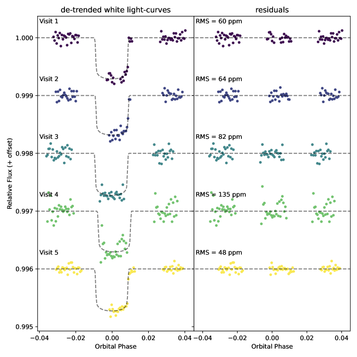
Figure 1:

Table 2:

Mid-point [BJD+2450000]	Analisys A	Analisys B
Visit 1	$8888.89348\pm 0.00016$	$8888.8921\pm 0.0012$
Visit 2	$8947.47386\pm 0.00029$	$8947.4730\pm 0.0012$
Visit 3	$9120.9646\pm 0.0023$	$9120.9626\pm 0.0018$
Visit 4	$9179.542\pm 0.004$	$9179.5435\pm 0.0021$
Visit 5	$9269.66962\pm 0.00010$	$9269.6680\pm 0.0012$
(Rp/Rs)2 [ppm]
Visit 1	663 $\pm$ 21	-
Visit 2	635 $\pm$ 26	-
Visit 3	676 $\pm$ 27	-
Visit 4	656 $\pm$ 36	-
Visit 5	676 $\pm$ 16	-
Combined	665.2 $\pm$ 11.7	642.6 $\pm$ 10.8

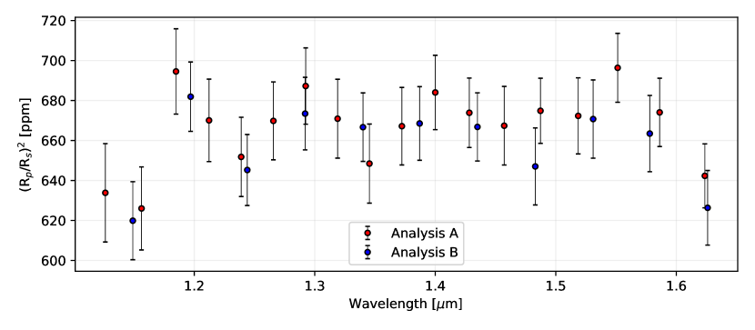
Figure 2: Transmission spectra of L98-59 b using the two independent methods described in Section 2. Each of the two spectra is the weighted average of the five single visits.

Table 3: Derived 1D spectra ((R_p/R_s)²) from the five visits of L98-59b using the Analysis A.

Spectral bins [nm]	V1	V2	V3	V4	V5	Weighted Average [ppm]
1110.8 - 1141.6	$636\pm 65$	$600\pm 62$	$670\pm 57$	$617\pm 47$	$647\pm 51$	$634\pm 25$
1141.6 - 1170.9	$626\pm 63$	$664\pm 47$	$662\pm 39$	$596\pm 41$	$567\pm 52$	$626\pm 21$
1170.9 - 1198.8	$680\pm 46$	$724\pm 47$	$676\pm 48$	$657\pm 74$	$708\pm 39$	$695\pm 21$
1198.8 - 1225.7	$636\pm 38$	$642\pm 52$	$732\pm 75$	$711\pm 40$	$666\pm 45$	$670\pm 21$
1225.7 - 1252.2	$652\pm 57$	$600\pm 42$	$631\pm 38$	$686\pm 43$	$708\pm 47$	$652\pm 20$
1252.2 - 1279.1	$670\pm 44$	$586\pm 42$	$644\pm 44$	$745\pm 36$	$673\pm 62$	$670\pm 19$
1279.1 - 1305.8	$695\pm 41$	$649\pm 63$	$626\pm 46$	$700\pm 37$	$722\pm 37$	$687\pm 19$
1305.8 - 1332.1	$679\pm 40$	$569\pm 46$	$675\pm 43$	$677\pm 47$	$749\pm 45$	$671\pm 20$
1332.1 - 1358.6	$688\pm 53$	$635\pm 39$	$671\pm 49$	$580\pm 43$	$690\pm 42$	$648\pm 20$
1358.6 - 1386.0	$667\pm 57$	$558\pm 39$	$717\pm 36$	$726\pm 49$	$686\pm 45$	$667\pm 19$
1386.0 - 1414.0	$696\pm 44$	$612\pm 56$	$710\pm 35$	$626\pm 48$	$711\pm 35$	$684\pm 19$
1414.0 - 1442.5	$666\pm 60$	$666\pm 41$	$691\pm 32$	$664\pm 37$	$670\pm 36$	$674\pm 17$
1442.5 - 1471.9	$672\pm 52$	$693\pm 49$	$661\pm 37$	$643\pm 37$	$691\pm 52$	$667\pm 20$
1471.9 - 1502.7	$659\pm 40$	$652\pm 37$	$717\pm 33$	$665\pm 31$	$670\pm 48$	$675\pm 16$
1502.7 - 1534.5	$677\pm 56$	$675\pm 44$	$722\pm 42$	$611\pm 35$	$707\pm 42$	$672\pm 19$
1534.5 - 1568.2	$683\pm 38$	$751\pm 48$	$687\pm 34$	$700\pm 32$	$675\pm 48$	$696\pm 17$
1568.2 - 1604.2	$658\pm 43$	$638\pm 38$	$680\pm 33$	$727\pm 39$	$663\pm 39$	$674\pm 17$
1604.2 - 1643.2	$665\pm 49$	$632\pm 30$	$647\pm 37$	$636\pm 29$	$654\pm 45$	$642\pm 16$

Table 4:

Spectral bins [nm]	(Rp/Rs)2 [ppm]
1125.0 - 1173.0	$620\pm 20$
1173.0 - 1220.5	$682\pm 17$
1220.5 - 1268.0	$645\pm 18$
1268.0 - 1316.0	$673\pm 18$
1316.0 - 1363.5	$667\pm 17$
1363.5 - 1411.0	$669\pm 18$
1411.0 - 1459.0	$667\pm 17$
1459.0 - 1507.0	$647\pm 19$
1507.0 - 1554.5	$671\pm 20$
1554.5 - 1602.0	$663\pm 19$
1602.0 - 1650.0	$626\pm 19$

4 Discussion

4.1 Plausible planetary scenarios

The transmission spectra do not show apparent modulation. The data are consistent with a flat spectrum where the transit depth does not change with wavelength with $\chi^{2}=17.8$ for a degree of freedom of 17. This means that the transmission spectra are consistent with a planet without any atmosphere (i.e., a bare-rock planet), or a planet with an atmosphere and high-altitude clouds or haze. For comparison, we have calculated the spectra of cloud-free H₂-dominated atmospheres with solar-abundance H₂O or CH₄, and they are clearly ruled out by the observed spectra (Fig. 3).

We have also tested whether the transmission spectrum of L98-59b would be consistent with a high mean molecular weight atmosphere. We found the spectra to be consistent with a CO₂-dominated atmosphere with $\chi^{2}=21.0$ (Fig. 3). Interestingly, the transmission spectrum H₂O-dominated atmosphere. We found that an H₂O-dominated atmosphere without clouds or haze would be . The reason for this potential inconsistency is that an H₂O-dominated atmosphere should cause a rise in the transit depth at $\sim 1.4\ \mu$m, which is absent from the data. This finding is somewhat surprising because an H₂O-dominated atmosphere was one of the most likely scenarios for this planet prior to the observations (Demangeon et al., 2021). On the other hand, the observed spectra can be consistent with an H₂O-dominated atmosphere if clouds are included , similar to the case of GJ 1214 b (Kreidberg et al., 2014).

To explore the potential atmospheric scenarios of the planet in a more systematic way, we used Tau-REx (Al-Refaie et al., 2021) to run a statistical inverse process to reveal the range of atmospheric conditions that would be consistent with the observed transmission spectrum. We adopted the results from Analysis A in the spectral retrieval. We assumed that the background atmosphere was dominated by molecular hydrogen and helium, but also allowed any gas of interest to take a mixing ratio of (almost) unity, effectively allowing, for example, an H₂O-, CO₂- or N₂-dominated atmosphere. We considered a broad range of molecules as candidate trace gases, including H₂O, CH₄, CO₂, CO, and HCN. Given the relatively narrow spectral range probed, we assumed an isothermal temperature profile and molecular abundances constant with pressure. We set uniform priors to the fitted parameters, which are: the mixing ratios of the molecules ($log(10^{-12})-log(10^{-0.1})$), the temperature (100 – 800 K), the radius of the planet (0.038 – 0.15 $R_{\mathrm{Jup}}$), and the cloud top pressure ($10^{-3}-10^{7}$ Pa). The retrieval model additionally has the opacity contribution from Rayleigh scattering and collision-induced absorption from H₂-H₂ and H₂-He pairs.

The spectral retrieval suggested an interesting scenario that involves an H₂-dominated atmosphere, clouds at $\sim 10^{3}$ Pa, and substantial presence of HCN (see Appendix C for the posterior distributions). The volume mixing ratio (VMR) of HCN is not well-constrained, but rather, the likelihood for higher values (>10^-2.5) is greater than lower values. Meanwhile, the retrieval disfavors any presence of H₂O or CH₄, and does not yield any constraints on CO, CO₂, or N₂ (Appendix C).

Table 5:

Scenario	log(EV)
H2-dominated atmosphere $+$ clouds $+$ HCN	165.44 $\pm$ 0.09
H2-dominated atmosphere $+$ clouds $+$ H2O $+$ CH4 $+$ HCN $+$ CO2 $+$ CO $+$ N2	165.27 $\pm$ 0.09
Fully clouded - flat spectrum	164.87 $\pm$ 0.09
CO2-dominated atmosphere cloud free	164.86 $\pm$ 0.09
H2O-dominated atmosphere $+$ clouds	164.86 $\pm$ 0.09
H2O-dominated atmosphere cloud free	160.93 $\pm$ 0.09

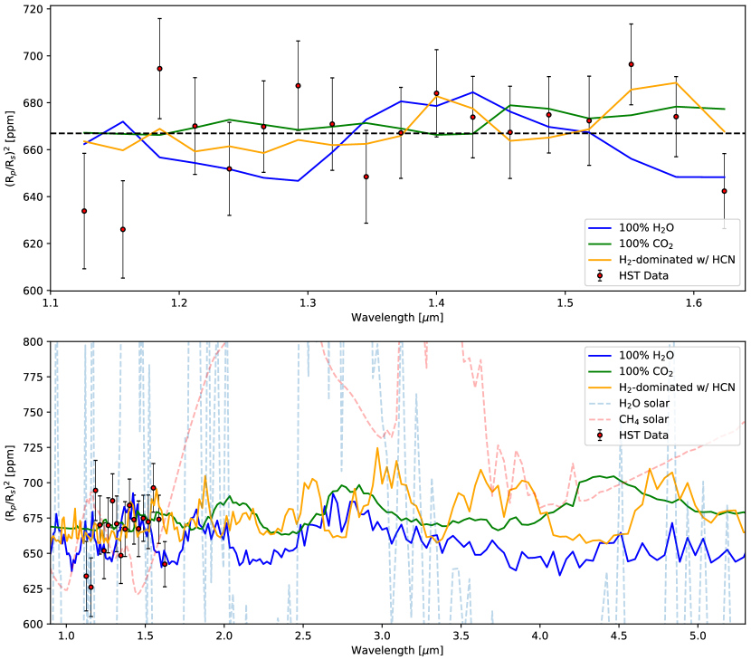
Figure 3: Top panel: Transmission spectrum of L98-59 b in comparison with model scenarios. The scenarios of an H₂O- or CO₂-dominated atmosphere assume that the atmosphere does not have clouds or haze and has a temperature of the planet’s equilibrium temperature. The H₂-dominated atmosphere model is the model calculated from the median of the posterior distribution shown in Fig. 5. This model has HCN with a volume mixing ratio of 360 parts per million and clouds at $10^{3}$ Pa in the atmosphere. Bottom panel: The HST data (Tsiaras et al., 2019; Benneke et al., 2019) comparing with atmospheric models of L98-59 b in the context of JWST observations. The dashed lines show the models with an H₂-dominated atmosphere and solar-abundance water and methane for comparison – these models are ruled out by the current data. The models permitted by the transmission spectrum reported here can be distinguished with JWST observations in $\sim 1.5-5\ \mu$m.

4.2 Stellar activity

While the initial discovery paper for the L98-59 planets indicated that no stellar variability was detected (Kostov et al., 2019), at least one flare is seen in subsequent TESS observations, and evidence of activity was identified in radial velocity data observations (Cloutier et al., 2019; Demangeon et al., 2021). Stellar activity can potentially mimic or mask the detection of at atmospheric signal in transmission spectra (Pont et al., 2008; Bean et al., 2010; Sing et al., 2011; Aigrain et al., 2012; Huitson et al., 2013; Jordán et al., 2013; Kreidberg et al., 2014; McCullough et al., 2014; Barstow et al., 2015; Nikolov et al., 2015; Herrero et al., 2016; Zellem et al., 2017; Rackham et al., 2018, 2019; Barclay et al., 2021). This is a particular challenge for early-mid M-dwarf stars where the residuals from stellar H₂O absorption can cause issues in the interpretation of data from $1.1-1.7\ \mu$m. The rotation rate of L98-59 is slow, likely in the region of 80 days (Cloutier et al., 2019; Demangeon et al., 2021). Therefore, the star rotates minimally during the 0.9 hour transit of L98-59 b. This makes a potential contamination signal somewhat less likely. However, even slowly rotating spotted stars are not immune to contaminated transmission spectra owing to the transit light source effect (Rackham et al., 2018).

All of the five observations of L98-59 b have consistent transmission spectra, which provides confidence that a single observation does not dominate the combined data and bias the conclusions (Appendix B). Furthermore, the characteristic bump of a contaminated spectrum at 1.4 $\mu$m due to H₂O in the stellar atmosphere (Barclay et al., 2021) is not observed for this planet. Therefore, while we cannot rule out that our observations contain some level of uncorrected stellar signal, we do not see any evidence for this.

4.3 Prospects of future studies

L98-59 b is currently the lowest-mass exoplanet measured through stellar radial velocities, and the uncertainties of the measured planetary mass and radius permit the planetary scenarios of a rocky body without any substantial gas or ice, a planet with $\sim 20\%$ water by mass, or a planet with a small H₂/He gas layer (Demangeon et al., 2021). It is thus particularly interesting to find out whether the planet has an atmosphere. Basic theoretical models suggest that sub-Earths in 2-day orbits should not have an atmosphere (e.g., Zahnle & Catling, 2017). However, these models do not include many effects that might allow small, highly irradiated planets to exhibit an atmosphere, for example the low escape efficiency for CO₂-dominated atmospheres (Tian, 2009; Johnstone et al., 2021). It is also plausible that the planet has retained some volatile through the early evolution (e.g., Kite & Schaefer, 2021) or has a secondary atmosphere from volcanic outgassing (e.g., Kite & Barnett, 2020). However, non-thermal escape processes may be very effective in removing the secondary atmosphere (e.g., Dong et al., 2018), and moreover, volcanic outgassing may shut down quickly on sub-Earth-mass planets (Kite et al., 2009).

If the planet does not have an atmosphere, its rocky surface could be spectroscopically detectable via Si-O features in $7-13\ \mu$m (Hu et al., 2012). Similar to the case of LHS 3844 b (Kreidberg et al., 2019), thermal emission spectroscopy using JWST’s MIRI instrument may detect the signatures of ultramafic, basaltic, and granitoid surfaces on this planet and reveal its geologic histories.

If the planet is a water world, it should have a steam atmosphere given the level of irradiation (e.g., Turbet et al., 2020). A cloudless H₂O atmosphere is not favored by the transmission spectra reported here, but is not ruled out. Theoretical calculations suggest that the escape efficiency for pure-H₂O atmospheres is high, similar to that for pure-H₂ atmospheres, disfavoring retention of a pure-H₂O atmosphere (Johnstone, 2020). A CO₂-dominated atmosphere built up by volcanic outgassing would be consistent with the transmission spectra. Because of L98-59 b’s low mass, this scenario would require that the planet start with much more CO₂ per unit mass than Earth or Venus according to the modeling of Kite & Barnett (2020). Therefore, if a CO₂-dominated atmosphere is detected in future, it would have major implications for the distribution and radial transport of Life-Essential Volatile Elements (LEVEs) including carbon to distances close to the star (Dasgupta & Grewal, 2019). The photometric precision achieved in this study is $\sim 20$ ppm per spectral channel, and a substantial improvement over this using HST may be very hard or inefficient. Fig. 3 suggests that a precision of $\sim 20$ ppm in $1.5-5\ \mu$m at a moderate spectral resolution, which should be within the reach of the instruments on JWST (e.g., Beichman et al., 2014), could detect such a non-H₂-dominated atmosphere on the planet and characterize its bulk composition. Because of L98-59 b’s small radius and known mass, such observations could provide a particularly powerful test for the models of planet-mass-dependent atmospheric retention and evolution on small planets.

Lastly, let us consider an H₂-dominated atmosphere having HCN and clouds. This scenario is favored by the retrieval of the transmission spectra as the statistical convergence tries to find the best model that fits the bump at 1.55 $\mu$m. The retrieval selects HCN in an H₂-dominated atmosphere and then it also invokes a cloud deck to produce an otherwise flat spectrum. This H₂-dominated atmosphere cannot be massive because, for the equilibrium temperature of $\sim 600$ K, an H₂-dominated atmosphere would already have a thickness of $0.4\ R_{\oplus}$ from 0.001 to 1 bar. To keep the H₂-dominated atmosphere small but existing is a fine-tuning problem as there is no known feedback mechanism that stabilizes the mass of the atmosphere. Is a small H₂-dominated atmosphere a plausible scenario from the atmospheric evolution point of view? It is possible that most of the initial endowment of hydrogen has been lost during early evolutions (e.g, Misener & Schlichting, 2021), and most of the remaining hydrogen is partitioned into the magma ocean (Kite et al., 2020; Gaillard et al., 2022). Volcanoes can release H₂-dominated gases into the atmosphere from the mantle (Liggins et al., 2020), and outgassing from impactors may also release H₂-dominated gases (Schaefer & Fegley, 2017). Therefore, it would be worthwhile to pursue the hint of HCN suggested in this scenario. HCN is a common photochemical product in temperate, H₂-dominated atmospheres (Hu, 2021) as well as in hot, N₂-dominated atmospheres (Miguel, 2019). Warm atmospheres on rocky exoplanets with volcanic outgassing could also have HCN (Swain et al., 2021). There have been debated reports of HCN from exoplanet transit observations (Tsiaras et al., 2016b; Swain et al., 2021), and here, the rise of the transit depth between $1.5-1.6\ \mu$m has been found by two data analyses and is most naturally explained as the HCN absorption (Fig. 3). This HCN, along with other possible scenarios discussed above, could be confirmed or refuted by observing the planet at longer wavelengths.

The other two detected planets in the L98-59 system (planets c and d) have been observed by HST within the program 15856 and the findings will be reported in a separate paper (Barclay et al. in prep). Moreover, JWST will observe the planets c and d in $0.6-5\ \mu$m through multiple programs in Cycle 1. The L98-59 system is poised to become one of best characterized exoplanetary systems with multiple small planets. Comparing the transmission spectra of the three planets could reveal system-wide trends in the atmospheric composition and thus volatile retention.

5 Conclusion

In the paper, we report the transmission spectra of the warm sub-Earth-sized exoplanet L98-59 b in $1.1-1.7\ \mu$m, obtained by multiple-visit observations of the HST. We applied two independent data analysis pipelines and obtained consistent results. Combining five visits, we achieved a photometric precision of $\sim 20$ ppm per spectral channel, with 18 channels in $1.1-1.7\ \mu$m ($R\sim 50$), making the transmission spectrum reported here one of the most precise measurements from an exoplanet (e.g., Kreidberg et al., 2014; Tsiaras et al., 2019; Benneke et al., 2019). The spectrum does not show significant modulation, and thus rules out a cloud-free H₂-dominated atmosphere with solar abundance of H₂O or CH₄. The spectrum also does not favor a cloud-free H₂O-dominated atmosphere. In addition to the null hypothesis (i.e., a bare-rock planet or an atmosphere with high-altitude clouds or haze), the spectrum is consistent with a CO₂-dominated atmosphere or a small H₂-dominated atmosphere with HCN and clouds/haze. JWST observations of the planet at the precision of $\sim 20$ ppm per spectral channel in a wide wavelength range could test these atmospheric scenarios and thus determine the nature of the planet. As a sub-Earth-sized planet, L98-59 b provides a valuable opportunity to test the volatile retention and evolution on small and irradiated exoplanets.

Appendix A

Table 6: Spectral bins and limb darkening coefficients used in the Analysis A.

Spectral bins [nm]	a1	a2	a3	a4
1110.8 - 1141.6	1.28798093	-1.05907762	0.51823029	-0.0874053
1141.6 - 1170.9	1.28615323	-1.08744839	0.54951993	-0.09832113
1170.9 - 1198.8	1.29932409	-1.153228	0.62233941	-0.12612099
1198.8 - 1225.7	1.31403541	-1.20359881	0.66336835	-0.13702432
1225.7 - 1252.2	1.3216165	-1.24503919	0.71220673	-0.15662467
1252.2 - 1279.1	1.31087844	-1.22725216	0.6846187	-0.14247216
1279.1 - 1305.8	1.33205793	-1.32351788	0.80287643	-0.19154707
1305.8 - 1332.1	1.33327291	-1.34653724	0.82282639	-0.19646486
1332.1 - 1358.6	1.35830426	-1.43403262	0.91975243	-0.23435426
1358.6 - 1386.0	1.35014645	-1.4334713	0.9180878	-0.23234897
1386.0 - 1414.0	1.34613423	-1.44645255	0.93259913	-0.23707517
1414.0 - 1442.5	1.34866834	-1.47233056	0.95865921	-0.24580419
1442.5 - 1471.9	1.38009113	-1.58464562	1.09298133	-0.30172869
1471.9 - 1502.7	1.34297544	-1.51871236	1.02049438	-0.27172675
1502.7 - 1534.5	1.31575231	-1.47873437	0.97919057	-0.25523316
1534.5 - 1568.2	1.32973852	-1.56395607	1.08417177	-0.29880839
1568.2 - 1604.2	1.29595229	-1.52289987	1.04537638	-0.28498663
1604.2 - 1643.2	1.28150047	-1.58351836	1.14303257	-0.32898329

Appendix B Single-visit transmission spectra

Following the extraction and correction of the white light curves (see Sec. 2 and Sec. 3), we fitted the spectral light curves to derive the 1D transmission spectrum. Fig. 4 shows the 1D transmission spectrum derived by using Analysis A for each of the five visits and and the combined weighted average.

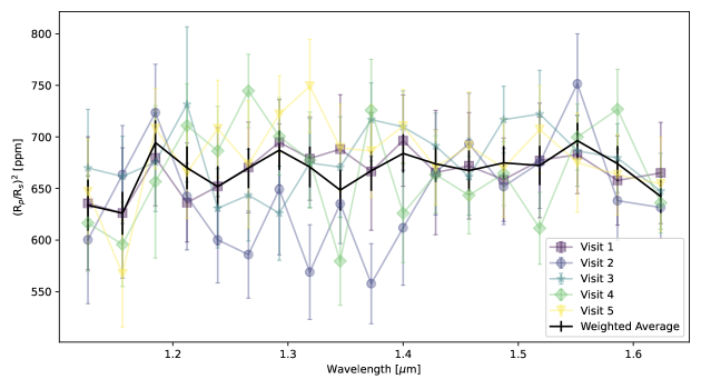
Figure 4: Colored : calculated 1D transmission spectrum of L98-59 b for each of the five HST visits resulting from the data analysis A described in Sec. 2. Black : weighted average combined transmission spectrum.

Table 7:

Spectral bins [nm]	RMS [ppm]	$\overline{\chi^{2}}$	$\overline{\sigma}$	R2
1110.8 - 1141.6	170 $\pm$ 16	1.062 $\pm$ 0.004	1.17 $\pm$ 0.11	0.21 $\pm$ 0.08
1141.6 - 1170.9	155 $\pm$ 22	1.066 $\pm$ 0.008	1.09 $\pm$ 0.16	0.08 $\pm$ 0.04
1170.9 - 1198.8	152 $\pm$ 13	1.066 $\pm$ 0.005	1.10 $\pm$ 0.09	0.16 $\pm$ 0.08
1198.8 - 1225.7	170 $\pm$ 57	1.062 $\pm$ 0.004	1.25 $\pm$ 0.42	0.15 $\pm$ 0.05
1225.7 - 1252.2	137 $\pm$ 12	1.066 $\pm$ 0.005	1.02 $\pm$ 0.09	0.13 $\pm$ 0.06
1252.2 - 1279.1	147 $\pm$ 22	1.062 $\pm$ 0.004	1.11 $\pm$ 0.17	0.13 $\pm$ 0.07
1279.1 - 1305.8	135 $\pm$ 6	1.064 $\pm$ 0.008	1.04 $\pm$ 0.04	0.12 $\pm$ 0.05
1305.8 - 1332.1	136 $\pm$ 7	1.064 $\pm$ 0.005	1.05 $\pm$ 0.05	0.12 $\pm$ 0.08
1332.1 - 1358.6	145 $\pm$ 9	1.064 $\pm$ 0.005	1.11 $\pm$ 0.08	0.10 $\pm$ 0.02
1358.6 - 1386.0	152 $\pm$ 26	1.062 $\pm$ 0.004	1.17 $\pm$ 0.19	0.09 $\pm$ 0.05
1386.0 - 1414.0	144 $\pm$ 19	1.064 $\pm$ 0.005	1.10 $\pm$ 0.15	0.10 $\pm$ 0.06
1414.0 - 1442.5	137 $\pm$ 15	1.054 $\pm$ 0.012	1.05 $\pm$ 0.12	0.17 $\pm$ 0.08
1442.5 - 1471.9	140 $\pm$ 10	1.054 $\pm$ 0.015	1.09 $\pm$ 0.08	0.12 $\pm$ 0.07
1471.9 - 1502.7	126 $\pm$ 7	1.062 $\pm$ 0.004	1.00 $\pm$ 0.06	0.15 $\pm$ 0.06
1502.7 - 1534.5	135 $\pm$ 6	1.062 $\pm$ 0.004	1.08 $\pm$ 0.05	0.13 $\pm$ 0.05
1534.5 - 1568.2	137 $\pm$ 17	1.064 $\pm$ 0.005	1.11 $\pm$ 0.14	0.13 $\pm$ 0.07
1568.2 - 1604.2	122 $\pm$ 8	1.062 $\pm$ 0.004	1.01 $\pm$ 0.06	0.14 $\pm$ 0.08
1604.2 - 1643.2	132 $\pm$ 25	1.064 $\pm$ 0.005	1.11 $\pm$ 0.21	0.10 $\pm$ 0.06

Appendix C Posterior distributions

The interpretation of the 1D spectrum shown in Fig. 2 has led to multiple scenarios that cannot be excluded. However, if the planet retains a light atmosphere, i.e. an H₂-dominated atmosphere, the statistical interpretation of the spectrum suggests that a significant amount of HCN might be present. We show the median-fit model from the spectral retrieval in Fig. 3 (orange line) and report the full posterior distributions here in Fig. 5.

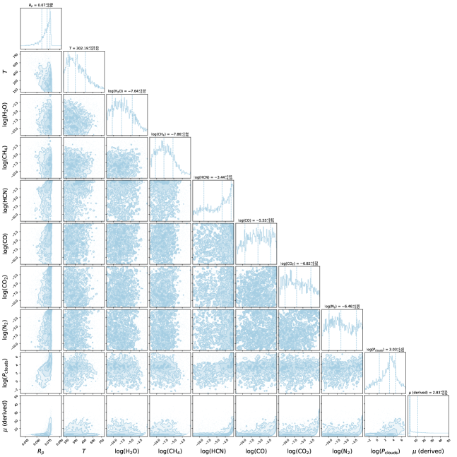
Figure 5: Posterior distributions of the retrieval on the 1D transmission spectrum of L98-59 b. The result suggests a light atmosphere (H₂-dominated) with clouds or haze and also hints the presence of HCN. The volume mixing ratio (VMR) of HCN has a distribution peak toward high values, but is otherwise not well constrained. All the other gases considered in the fitting show VMR distributions toward low values or completely flat, suggesting their absence in the atmosphere or a presence below the cloud deck not detectable by transmission spectroscopy.

References

- Aigrain et al. (2012) Aigrain, S., Pont, F., & Zucker, S. 2012, MNRAS, 419, 3147, doi: 10.1111/j.1365-2966.2011.19960.x
- Al-Refaie et al. (2021) Al-Refaie, A. F., Changeat, Q., Waldmann, I. P., & Tinetti, G. 2021, ApJ, 917, 37, doi: 10.3847/1538-4357/ac0252
- Allard et al. (2003) Allard, F., Guillot, T., Ludwig, H.-G., et al. 2003, in Brown Dwarfs, ed. E. Martín, Vol. 211, 325
- Barclay et al. (2021) Barclay, T., Kostov, V. B., Colón, K. D., et al. 2021, AJ, 162, 300, doi: 10.3847/1538-3881/ac2824
- Barstow et al. (2015) Barstow, J. K., Aigrain, S., Irwin, P. G. J., Kendrew, S., & Fletcher, L. N. 2015, MNRAS, 448, 2546, doi: 10.1093/mnras/stv186
- Bean et al. (2010) Bean, J. L., Miller-Ricci Kempton, E., & Homeier, D. 2010, Nature, 468, 669, doi: 10.1038/nature09596
- Beichman et al. (2014) Beichman, C., Benneke, B., Knutson, H., et al. 2014, Publications of the Astronomical Society of the Pacific, 126, 1134
- Benneke et al. (2019) Benneke, B., Wong, I., Piaulet, C., et al. 2019, ApJ, 887, L14, doi: 10.3847/2041-8213/ab59dc
- Buchner et al. (2014) Buchner, J., Georgakakis, A., Nandra, K., et al. 2014, A&A, 564, A125, doi: 10.1051/0004-6361/201322971
- Claret (2000) Claret, A. 2000, A&A, 363, 1081
- Cloutier et al. (2019) Cloutier, R., Astudillo-Defru, N., Bonfils, X., et al. 2019, A&A, 629, A111, doi: 10.1051/0004-6361/201935957
- Damiano et al. (2017) Damiano, M., Morello, G., Tsiaras, A., Zingales, T., & Tinetti, G. 2017, AJ, 154, 39, doi: 10.3847/1538-3881/aa738b
- Dasgupta & Grewal (2019) Dasgupta, R., & Grewal, D. S. 2019, Deep carbon, 4
- De Wit et al. (2018) De Wit, J., Wakeford, H. R., Lewis, N. K., et al. 2018, Nature Astronomy, 2, 214
- Demangeon et al. (2021) Demangeon, O. D. S., Zapatero Osorio, M. R., Alibert, Y., et al. 2021, A&A, 653, A41, doi: 10.1051/0004-6361/202140728
- Deming et al. (2013) Deming, D., Wilkins, A., McCullough, P., et al. 2013, ApJ, 774, 95, doi: 10.1088/0004-637X/774/2/95
- Dong et al. (2018) Dong, C., Jin, M., Lingam, M., et al. 2018, Proceedings of the National Academy of Sciences, 115, 260
- Evans et al. (2016) Evans, T. M., Sing, D. K., Wakeford, H. R., et al. 2016, ApJ, 822, L4, doi: 10.3847/2041-8205/822/1/L4
- Feroz & Hobson (2007) Feroz, F., & Hobson, M. P. 2007
- Feroz et al. (2009) Feroz, F., Hobson, M. P., & Bridges, M. T. B. 2009
- Feroz et al. (2013) Feroz, F., Hobson, M. P., Cameron, E., & Pettitt, A. N. 2013
- Foreman-Mackey et al. (2013) Foreman-Mackey, D., Hogg, D. W., Lang, D., & Goodman, J. 2013, PASP, 125, 306, doi: 10.1086/670067
- Fraine et al. (2014) Fraine, J., Deming, D., Benneke, B., et al. 2014, Nature, 513, 526, doi: 10.1038/nature13785
- Freedman et al. (2014) Freedman, R. S., Lustig-Yaeger, J., Fortney, J. J., et al. 2014, ApJS, 214, 25, doi: 10.1088/0067-0049/214/2/25
- Freedman et al. (2008) Freedman, R. S., Marley, M. S., & Lodders, K. 2008, ApJS, 174, 504, doi: 10.1086/521793
- Gaillard et al. (2022) Gaillard, F., Bernadou, F., Roskosz, M., et al. 2022, Earth and Planetary Science Letters, 577, 117255
- Haynes et al. (2015) Haynes, K., Mandell, A. M., Madhusudhan, N., Deming, D., & Knutson, H. 2015, ApJ, 806, 146, doi: 10.1088/0004-637X/806/2/146
- Herrero et al. (2016) Herrero, E., Ribas, I., Jordi, C., et al. 2016, A&A, 586, A131, doi: 10.1051/0004-6361/201425369
- Horne (1986) Horne, K. 1986, Publications of the Astronomical Society of the Pacific, 98, 609, doi: 10.1086/131801
- Hu (2021) Hu, R. 2021, The Astrophysical Journal, 921, 27
- Hu et al. (2012) Hu, R., Ehlmann, B. L., & Seager, S. 2012, The Astrophysical Journal, 752, 7
- Huitson et al. (2013) Huitson, C. M., Sing, D. K., Pont, F., et al. 2013, MNRAS, 434, 3252, doi: 10.1093/mnras/stt1243
- Johnstone (2020) Johnstone, C. P. 2020, ApJ, 890, 79, doi: 10.3847/1538-4357/ab6224
- Johnstone et al. (2021) Johnstone, C. P., Lammer, H., Kislyakova, K. G., Scherf, M., & Güdel, M. 2021, Earth and Planetary Science Letters, 576, 117197, doi: 10.1016/j.epsl.2021.117197
- Jordán et al. (2013) Jordán, A., Espinoza, N., Rabus, M., et al. 2013, ApJ, 778, 184, doi: 10.1088/0004-637X/778/2/184
- Kempton et al. (2017) Kempton, E. M. R., Lupu, R., Owusu-Asare, A., Slough, P., & Cale, B. 2017, PASP, 129, 044402, doi: 10.1088/1538-3873/aa61ef
- Kite & Barnett (2020) Kite, E. S., & Barnett, M. N. 2020, Proceedings of the National Academy of Sciences, 117, 18264
- Kite et al. (2020) Kite, E. S., Fegley Jr, B., Schaefer, L., & Ford, E. B. 2020, The Astrophysical Journal, 891, 111
- Kite et al. (2009) Kite, E. S., Manga, M., & Gaidos, E. 2009, ApJ, 700, 1732, doi: 10.1088/0004-637X/700/2/1732
- Kite & Schaefer (2021) Kite, E. S., & Schaefer, L. 2021, ApJ, 909, L22, doi: 10.3847/2041-8213/abe7dc
- Knutson et al. (2014) Knutson, H. A., Benneke, B., Deming, D., & Homeier, D. 2014, Nature, 505, 66, doi: 10.1038/nature12887
- Knutson et al. (2007) Knutson, H. A., Charbonneau, D., Noyes, R. W., Brown, T. M., & Gilliland, R. L. 2007, ApJ, 655, 564, doi: 10.1086/510111
- Kostov et al. (2019) Kostov, V. B., Schlieder, J. E., Barclay, T., et al. 2019, AJ, 158, 32, doi: 10.3847/1538-3881/ab2459
- Kreidberg (2015) Kreidberg, L. 2015, PASP, 127, 1161, doi: 10.1086/683602
- Kreidberg et al. (2014) Kreidberg, L., Bean, J. L., Désert, J.-M., et al. 2014, Nature, 505, 69, doi: 10.1038/nature12888
- Kreidberg et al. (2018) Kreidberg, L., Line, M. R., Parmentier, V., et al. 2018, AJ, 156, 17, doi: 10.3847/1538-3881/aac3df
- Kreidberg et al. (2019) Kreidberg, L., Koll, D. D., Morley, C., et al. 2019, Nature, 573, 87
- Liggins et al. (2020) Liggins, P., Shorttle, O., & Rimmer, P. B. 2020, Earth and Planetary Science Letters, 550, 116546
- Lupu et al. (2014) Lupu, R. E., Zahnle, K., Marley, M. S., et al. 2014, ApJ, 784, 27, doi: 10.1088/0004-637X/784/1/27
- McCullough & MacKenty (2012) McCullough, P., & MacKenty, J. 2012, Considerations for using Spatial Scans with WFC3, Space Telescope WFC Instrument Science Report
- McCullough et al. (2014) McCullough, P. R., Crouzet, N., Deming, D., & Madhusudhan, N. 2014, ApJ, 791, 55, doi: 10.1088/0004-637X/791/1/55
- Miguel (2019) Miguel, Y. 2019, Monthly Notices of the Royal Astronomical Society, 482, 2893
- Misener & Schlichting (2021) Misener, W., & Schlichting, H. E. 2021, Monthly Notices of the Royal Astronomical Society, 503, 5658
- Morello et al. (2020) Morello, G., Claret, A., Martin-Lagarde, M., et al. 2020, AJ, 159, 75, doi: 10.3847/1538-3881/ab63dc
- Mugnai et al. (2021) Mugnai, L. V., Modirrousta-Galian, D., Edwards, B., et al. 2021, The Astronomical Journal, 161, 284
- Nikolov et al. (2015) Nikolov, N., Sing, D. K., Burrows, A. S., et al. 2015, MNRAS, 447, 463, doi: 10.1093/mnras/stu2433
- Pont et al. (2008) Pont, F., Knutson, H., Gilliland, R. L., Moutou, C., & Charbonneau, D. 2008, MNRAS, 385, 109, doi: 10.1111/j.1365-2966.2008.12852.x
- Rackham et al. (2018) Rackham, B. V., Apai, D., & Giampapa, M. S. 2018, ApJ, 853, 122, doi: 10.3847/1538-4357/aaa08c
- Rackham et al. (2019) —. 2019, AJ, 157, 96, doi: 10.3847/1538-3881/aaf892
- Ricker et al. (2015) Ricker, G. R., Winn, J. N., Vanderspek, R., et al. 2015, Journal of Astronomical Telescopes, Instruments, and Systems, 1, 014003, doi: 10.1117/1.JATIS.1.1.014003
- Schaefer & Fegley (2017) Schaefer, L., & Fegley, B. 2017, The Astrophysical Journal, 843, 120
- Sing et al. (2011) Sing, D. K., Pont, F., Aigrain, S., et al. 2011, MNRAS, 416, 1443, doi: 10.1111/j.1365-2966.2011.19142.x
- Sing et al. (2016) Sing, D. K., Fortney, J. J., Nikolov, N., et al. 2016, Nature, 529, 59, doi: 10.1038/nature16068
- Sivia & Skilling (2006) Sivia, D., & Skilling, J. 2006, Data Analysis A Bayesian Tutorial (Oxford University Press)
- Skilling (2004) Skilling, J. 2004, in American Institute of Physics Conference Series, ed. R. Fischer, R. Preuss, & U. V. Toussaint, Vol. 735, 395–405
- Skilling (2006) Skilling, J. 2006, Bayesian Analysis, 1, 833
- Swain et al. (2008) Swain, M. R., Vasisht, G., & Tinetti, G. 2008, Nature, 452, 329, doi: 10.1038/nature06823
- Swain et al. (2009) Swain, M. R., Tinetti, G., Vasisht, G., et al. 2009, ApJ, 704, 1616, doi: 10.1088/0004-637X/704/2/1616
- Swain et al. (2021) Swain, M. R., Estrela, R., Roudier, G. M., et al. 2021, The Astronomical Journal, 161, 213
- Tian (2009) Tian, F. 2009, ApJ, 703, 905, doi: 10.1088/0004-637X/703/1/905
- Tsiaras et al. (2016a) Tsiaras, A., Waldmann, I. P., Rocchetto, M., et al. 2016a, ApJ, 832, 202, doi: 10.3847/0004-637X/832/2/202
- Tsiaras et al. (2019) Tsiaras, A., Waldmann, I. P., Tinetti, G., Tennyson, J., & Yurchenko, S. N. 2019, Nature Astronomy, 3, 1086, doi: 10.1038/s41550-019-0878-9
- Tsiaras et al. (2016b) Tsiaras, A., Rocchetto, M., Waldmann, I. P., et al. 2016b, ApJ, 820, 99, doi: 10.3847/0004-637X/820/2/99
- Tsiaras et al. (2018) Tsiaras, A., Waldmann, I. P., Zingales, T., et al. 2018, AJ, 155, 156, doi: 10.3847/1538-3881/aaaf75
- Turbet et al. (2020) Turbet, M., Bolmont, E., Ehrenreich, D., et al. 2020, Astronomy & Astrophysics, 638, A41
- Zahnle & Catling (2017) Zahnle, K. J., & Catling, D. C. 2017, ApJ, 843, 122, doi: 10.3847/1538-4357/aa7846
- Zellem et al. (2017) Zellem, R. T., Swain, M. R., Roudier, G., et al. 2017, ApJ, 844, 27, doi: 10.3847/1538-4357/aa79f5
- Zhang et al. (2018) Zhang, Z., Zhou, Y., Rackham, B. V., & Apai, D. 2018, The Astronomical Journal, 156, 178
- Zhou et al. (2017) Zhou, Y., Apai, D., Lew, B. W. P., & Schneider, G. 2017, AJ, 153, 243, doi: 10.3847/1538-3881/aa6481