Perceptual Grouping in Contrastive Vision-Language Models

Abstract

Recent advances in zero-shot image recognition suggest that vision-language models learn generic visual representations with a high degree of semantic information that may be arbitrarily probed with natural language phrases. Understanding an image, however, is not just about understanding what content resides within an image, but importantly, where that content resides. In this work we examine how well vision-language models are able to understand where objects reside within an image and group together visually related parts of the imagery. We demonstrate how contemporary vision and language representation learning models based on contrastive losses and large web-based data capture limited object localization information. We propose a minimal set of modifications that results in models that uniquely learn both semantic and spatial information. We measure this performance in terms of zero-shot image recognition, unsupervised bottom-up and top-down semantic segmentations, as well as robustness analyses. We find that the resulting model achieves state-of-the-art results in terms of unsupervised segmentation, and demonstrate that the learned representations are uniquely robust to spurious correlations in datasets designed to probe the causal behavior of vision models.

1 Introduction

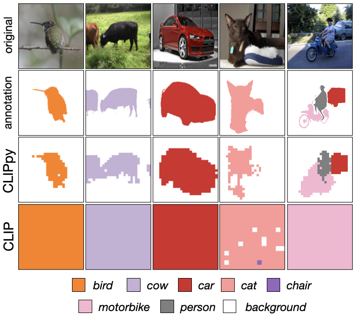
Figure 1: Semantic localization in contrastive VLMs. We measure the ability of vision-language models to predict a label at each spatial position in a zero shot manner based on the similarity of location tokens to the corresponding language tokens on selected examples. CLIP / ALIGN [50, 85] have minimal understanding of the spatial location of individual objects (row 4). Our proposed CLIPpy (row 3) predicts the label at locations that correspond closely to human annotation for semantic segmentation (row 2). All predictions were performed with no access to any segmentation data during training or inference. More visualizations in App. B.

Learning a representation for visual imagery requires resolving not only what resides within an image, but also where that information resides [72]. In many applications, knowledge of where information resides is sometimes more important than a precise description of the content [33, 98]. Hence, our ability to learn more generic and robust visual representations requires learning the geometry of visual semantics, and how visual information may be grounded by specific regions of the visual field.

While recent vision-language models trained under weak supervision demonstrate a remarkable ability to learn generic and transferable visual representations [50, 85, 117, 24], they showcase a profound inability to associate visual content with individual objects (Fig. 1, bottom row). In other words, models trained on large weakly-supervised data have a limited ability to group together visually related content [36]. Because the representations have a poor understanding of where an object resides, they easily conflate background with foreground content. Hence, the learned representations are unable to learn the spatial layout of a scene [97, 101], and are susceptible to learning spurious correlations between a semantic label and extraneous content [91, 65].

Recent work [113, 114] attempts to bridge this gap through grouping mechanisms under the same weakly supervised training paradigm, but focus more on foreground objects (neglecting background classes). Another direction is task specific unsupervised fine-tuning [126, 26] which loses the generic and transferable nature of these representations.

In this work, we explore vision-language models that learn from similar weakly labeled data, but a) retain the generic and transferable nature of features, and b) learns where all (background and foreground) visual content resides within an image. Unlike previous attempts using grouping specific architectures [113, 114] or dense human annotations [36, 38, 57], we explore a minimal set of modifications to existing CLIP models [85] that leads to grouping of visual imagery while retaining their weakly supervised and scalable training procedure. We find that two small adjustments – employing specific pretraining strategies and adjusting spatial feature aggregation – results in models that are equally effective in zero-shot image recognition, but also retain spatial information regarding object locations (see Fig. 1, 3rd row).

The resulting model termed CLIPpy exhibits perceptual grouping – that is, the ability to select and combine related visual signals into semantically meaningful regions [110, 72, 89]. Endowing models with perceptual grouping – whether in a bottom up (based solely on visual content) or top down (guided by external information, language in this case) manner – in learned representations has been a long standing goal in computer vision [70, 71]. In this work, our key contributions are as follows:

• Identify systematic failure of contrastive vision-language models [85, 50] to properly identify where objects reside within an image, and group semantically related content.

• Design a minimal set of changes to endow these model with perceptual grouping, resulting in state-of-the-art zero-shot segmentation without training on any segmentation data or performing task specific fine-tuning.

• Emergence of localization ability in our models uniquely leads to robustness to counterfactual manipulations. The degree of robustness matches if not surpasses previous state-of-the-art supervised learning methods employing specialized training methodologies.

2 Related Work

Vision-language models for grounding. Contrastive language image pre-training [85] (CLIP) led to a range of follow up work performing open-vocabulary detection [38, 51, 58, 59, 120, 28] or segmentation [36, 57, 122]. While these methods leverage dense human annotations for training, an alternate line of works [113, 114, 126, 115, 22] attempt to learn alignment between regions of images and language with only image level noisy captions for supervision. Their weak supervision allows better scalability (to more data) leading to learning more generic and transferable representations. In fact, multiple such works [113, 114, 126, 26, 57] perform zero-shot semantic segmentation. However, unlike [113, 114] geared to segment a fixed count of foreground objects, our proposed CLIPpy can better segment arbitrary object counts and background classes. In contrast to [126] using generic image level features, CLIPpy explicitly learns local features during training. Moreover, CLIPpy requires no dense human annotations or task-specific fine-tuning in contrast to [26, 57]. We also highlight how [113, 114, 26] perform grouping independent of language at inference - however CLIPpy can group conditioned on language, capturing variable object boundaries for different language prompts.

Multiple contemporary works also explore similar directions as CLIPpy, leveraging pre-trained vision-language models for various grouping tasks under weak supervision (no pixel level annotation) [123, 68, 13, 75, 9, 52]. Combining self-supervised methods that emerge grouping [12] with CLIP models [85] for cross-modal alignment is explored in [123] gaining notable improvements at object boundaries. A clustering mechanism containing learnable centres similar to [113] is combined with reconstruction and super-pixel alignment losses to achieve grouping in [68]. Learning decoder networks over a frozen CLIP backbone [85] with text to image patch similarity losses are explored in [13, 75] resulting in similar grouping behaviour. In contrast to these methods utilizing contrastive vision language training to emerge grouping, recent works [9, 52] also showcase how text-to-image generative models (particularly Stable Diffusion [90]) can be leveraged to perform visual grouping.

Component	CLIP [85]	CLIP†	CLIPpy
Image Backbone	ViT-B/16	ViT-B/16	ViT-B/16
Text Backbone	T-B	T-5	T-5
Image Init	Random	Random	DINO
Text Init	Random	Random	Sent T-5
Image Pooling	CLS	CLS	Max
Text Pooling	Avg	Avg	Avg
Dataset	300M∗	CC-12M	CC-12M
VOC mIoU (%)	16.4	17.5	50.8 ${}_{\text{{\color[rgb]{0,0.88,0}(+33.3)}}}$
VOC JS (%)	28.6	37.3	47.5 ${}_{\text{{\color[rgb]{0,0.88,0}(+10.2)}}}$

Table 1: We highlight the minimal differences of CLIPy from CLIP. CLIP^† is our implementation following train settings identical to CLIPpy. ^∗indicates OpenAI private data.

Figure 2: Architecture diagram. Images and captions are separately embedded into Euclidean spaces, where image features are spatially aggregated. A contrastive loss trains the aggregated image embedding to be close to the caption embedding. We demonstrate that two minimal design decisions (indicated in green) are of paramount importance for CLIP [85] models to perform perceptual grouping under image-level weak supervision.

Zero-shot semantic segmentation. A form of top-down grouping, this relatively new task [124, 48, 111, 8, 79, 45, 60, 3, 95] attempts to segment unseen classes, usually after a supervised training phase often involving dense annotation based supervision. Following two early representative works [111, 8], most later approaches [60, 39, 40, 53, 95, 102] formulate the task as a pixel-level zero-shot classification problem with a closed set vocabulary. While CLIPpy follows a similar pixel based formulation, in contrast, our method requires no dense human annotations for supervision, no task specific fine-tuning, and is open-vocabulary. Recent work [26, 58] also explores region-level classification leveraging pre-trained CLIP models [85], but unlike CLIPpy perform grouping independent of language during inference.

Unsupervised segmentation. Analogous to bottom-up grouping, these works perform class-agnostic segmentation within the visual modality with no explicit language alignment [12, 41, 31, 49, 73]. This topic has a long, rich history in human visual perception [110] and computer vision [70], and has been explored as means of generalizing to new visual domains [84, 71]. It is this goal that most closely inspires our work. Early efforts group pixels based on known spatially-local affinities [19, 96, 88], with subsequent methods leading to region proposal networks for object detection [103] and advances in semantic segmentation [1]. Recent methods employ self-supervision to learn perceptual grouping [18, 41] or object-centric groupings [29, 66, 109, 4, 44]. Our proposed CLIPpy demonstrates competitive performance, but additionally aligns groups to the language modality explicitly.

Learning robust visual representations. For a long time, ImageNet [23] accuracy was believed to provide a reasonable proxy for quality of learned visual representations [37, 55]. However, recent work highlights notable deficiencies in such learned representations [34, 87, 54] including sensitivity to low level textures, failure for domain shifts, and reliance on spurious correlations. These failures inspired a large literature to mitigate learning spurious correlations [91, 65, 2] by focusing on new optimization techniques. Progress on this issue may address parallel issues in fairness [21]. Resulting methods have largely focused on synthetic data, re-balancing data, and shaping learned embeddings [76, 65]. Nonetheless, theoretical results suggest pessimistic bounds unless additional structure informs the problem (see refs. in [91]). Therein, the structured output predictions of proposed CLIPpy provide another promising solution.

3 Methodology

We first set the stage by discussing established core architectures and the contrastive learning formulation. Next, we discuss modifications that are the focus of the analysis in this work. In particular, we discuss aggregation options, pre-training alternatives, and token sub-sampling.

3.1 Architecture and Training

We provide a quick overview of our architecture (Fig. 2). Consider a batch size $N$, spatial height $H$, spatial width $W$, and depth $D$. $X$ is a tensor that has a shape of $[N,H,W,D]$ and is the output of an image encoder. $Y$ is a tensor that is of shape $[N,D]$ and is the output of a text encoder.

Language Model. We employ a strong language model baseline derived from the transformer architecture [104] and implemented in T5 [86]. T5 models use an encoder-decoder architecture that is trained using a generative span corruption task, and have achieved state-of-the-art on a broad range of NLP tasks including GLUE [106] and Super-Glue [105]. We use the encoder only and discard the decoder part. We employ the T5-base which consists of 12 transformer layers, 12 attention heads, and 768 token channel dimensions.

Image Model. We explore two architectures for image featurization, CNN-based and Vision-Transformers, although we focus the majority of work on the latter. First, we employ the EfficientNet architecture [100] as a high performant CNN architecture, which has been used previously in vision-language models. The specifics of the meta-architecture were derived from considerations based on neural architecture search. Second, we employ the Vision Transformer (ViT) architecture [27]. We refer the reader to [27, 104] for details. Briefly, ViT is largely inherited from the NLP literature and consists of a hierarchical associative memory. Each layer, termed a transformer, is composed of a Multi-headed Self-Attention (MSA) layer followed by a 2-layer feed-forward multi-layer perceptron (MLP). The primary parameter of ViT is the patch size $P$ specifying the $P\times P$ patch of pixels constituting a token in the architecture.

Contrastive Representation Learning. Let $x_{i}$ and $y_{i}$ denote the image and text embeddings (post aggregation) of the $i$’th example in the batch. A contrastive loss may be specified as the cross entropy across a batch [85, 50]. The cross entropy is calculated between a one-hot encoding specifying the correspondence between the image and text examples, and a softmax-normalized distribution specifying the dot-product similarity between image and text embeddings.

$L=\underbrace{-\frac{1}{N}\sum_{i=1}^{N}\log{\frac{\exp(x_{i}^{\top}y_{i}/\tau)}{\sum_{j=1}^{N}\exp(x_{i}^{\top}y_{j}/\tau)}}}_{\text{image-to-text}}\,\,+\,\,\underbrace{-\frac{1}{N}\sum_{i=1}^{N}\log{\frac{\exp(y_{i}^{\top}x_{i}/\tau)}{\sum_{j=1}^{N}\exp(y_{i}^{\top}x_{j}/\tau)}}}_{\text{text-to-image}}$

The normalization for the image-to-text and text-to-image similarity is computed by summing over the potential matches (indexed by $j$) to the text and image examples within a batch, respectively. Note that $\tau$ is the temperature of the softmax for the normalization.

3.2 Aggregation

The goal of the aggregation method is to collapse the image embedding from a $[H,W,D]$ tensor to a $D$ dimensional vector. Average pooling across space is an established technique for ensuring that the final embedding is independent of the image resolution [99, 67], and has been adopted for CNN-based architectures in vision-language models [50]. Alternatively, maximum pooling has been explored, in particular with success for point clouds [83] and image-audio [42]. Another approach typical for ViT borrowed from language modeling [25] is the class token (CLS), which is prepended to the image patch tokens [27]. A class token learns an embedding that aggregates information across all patch tokens in order to predict the image label. The class token may be used to summarize the content for an entire image for ViT-based models [85, 12]. Subsequent work in vision-language models has explored learning pooling strategies [15, 115], heuristically selecting a set of similar neighbors [118] or learning attention-based mechanisms [117].

In this work we systematically explore these aggregation strategies. In early experiments we found that many complex strategies for aggregation yielded poor results (App. A.2). We found that the application of max pooling across the spatial dimensions – while extremely simple – was also by far the most effective (Sec. 4.5). We hypothesize that the success of max pooling may be due to the gradient updates being focused solely on a single spatial location, and not spread across all spatial dimensions.

Why Max Pooling? In particular, the max pooling operation allows pre-aggregation features (shaped $[N,H,W,D]$) to determine the spatial location for gradient updates at each step, conditioned on input images. Across different images containing a common object at different spatial locations, the model has to select a conservative and minimal set of spatial locations for gradient updates. At the same time, given the cross-modal contrastive train objective, the aggregated feature of each such image must be aligned towards a common language concept (i.e. related to the common object). We hypothesize that gradient updates at the common object’s spatial location is the simplest optimization for the train objective in this case, leading to observed perceptual grouping.

3.3 Pretraining

Language Model. For better sentence level representation, we utilize pre-training from Sentence-T5 [78] which adapts a T5 encoder to sentence level embedding using a contrastive objective. We select Sentence-T5 over auto-regressive models such as [25, 7] because this contrastive loss is aligned to our setup. The model is trained on Stanford Natural Language Inference (SNLI) dataset with 275K examples focused on entailment questions [6, 32].

Image Model. We investigate initializing the image model with several methods. First, we investigate initializing the image model using supervised pre-training and removing the final layer for logistic regression [37, 55]. We next investigate self-supervised methods derived from self-distillation (e.g. [12]). We focused on this latter direction because such models demonstrated impressive performance in terms of localization [12, 41]. All image pre-training is performed on ImageNet-1K [23] dataset.

Suitable Visual Pre-training. The visual encoder representation space can be viewed as containing per-image features (post-aggregation) vs per-spatial location features (pre-aggregation). We hypothesize that semantics tied boundaries of this representation space should operate at the latter granularity to induce perceptual grouping. Furthermore, we suggest that initializations facilitating the former will detriment grouping behaviour. In particular, visual pre-training strategies separating image-level representations by semantics (e.g. supervised ImageNet pre-training) will diminish perceptual grouping. Self-supervised pre-training strategies focused on more granular within image representations (e.g. [12]) will tend to enhance perceptual grouping. This hypothesis is empirically validated in ablations (see Table 8).

3.4 Visual Token Sub-Sampling

Motivated by vision transformers’ ability to process sequences of length different to train time, we generate higher resolution segmentations during inference by sampling more image patches. In order to increase robustness to such varying resolution, we utilize up to $2\times$ higher resolution images during training but randomly drop 80% of visual tokens to minimize additional compute overhead (similar to [43, 62]). While improving segmentations, this also provides training stability possibly due to its regularizing effect (see App. D).

3.5 Inference

CLIPpy performs inference under 3 different settings: a) classification, b) bottom-up grouping, and c) top-down grouping. On the visual modality, the first utilizes a spatially aggregated single per-image token while the latter two utilize sets of per-region tokens. Classification follows zero-shot analyses from [85] where the model is prompted at inference for a selection of labels (App. I for prompts). Bottom-up grouping follows a form of spectral clustering inspired by [12] (refer to their demo). PCA on image features (from visual encoder pre-aggregation) gives top n(=8) principal components, which are used as cluster centers. Each of those same image features are assigned to one of the n clusters based on proximity (cosine similarity) to the centers, resulting in n clusters (or groups). Top-down grouping employs zero shot analysis similar to [85], but at each spatial location, using the per-region tokens. This is similar to [35] and generates predictions across space exploiting the transitive property of our aggregation operations.

4 Experiments

Experimental Setup. We train our models on two datasets: Conceptual Captions 12M (CC-12M) [14] and High Quality Image Text Pairs (HQITP-134M) consisting of 12 million and 134 million image-text pairs, respectively (App. C for details). For both datasets, text is tokenized, and images resized and center cropped to 224$\times$224 pixels. We report results on EfficientNet-B5 employed by ALIGN [50], and ViT-B/16 employed by CLIP [85] although we focus more on the latter. We train models on 32 GPUs across 4 machines with PyTorch [80]. See App. D for more details. We evaluate across image classification, localization, and robustness tasks. For image classification, we employ the validation splits of ImageNet [23] and ImageNet-v2 [87], and for robustness we employ the test split of Waterbirds [91]. These datasets contain 1000, 1000, and 3 classes respectively. For segmentation tasks, we employ the validation splits of PASCAL VOC [30], ADE20K [125, 17], COCO [64], COCO (Obj) [64], and Cityscapes [20]. Each of these datasets contain 20, 150, 133, 80, and 27 labels, respectively.

Baselines for comparison. Given that most competitive baselines are trained on private datasets, we first attempt to reproduce results by training models on a corpus of image-text pairs. In more detail, we train on the public CC-12M dataset [14] to provide reproducible numbers and observe competitive performance given our data limitations. We also train on the larger HQITP-134M dataset to verify scalability.

We first measure the performance of CLIP [85] and ALIGN [50] on zero-shot image classification on ImageNet and ImageNet-v2. Table 2 highlights these results. We take this as a starting point for subsequent work. In the following experiments we attempt to address the following questions:

• What are the limitations of current vision-language models? (Fig. 1)

• Do we observe perceptual grouping in vision language models? (Tabs. 3, 4 and 6).

• How resilient are vision-language models to counterfactual manipulations? (Fig. 4).

• How important are each of the proposed model modifications? (Tabs. 7, 8, 9 and 10).

4.1 Limitations of vision-language models

Visual representations learned in vision-language models exhibit an impressive ability to generalize across tasks [85, 50]. However they also exhibit a profound shortcoming – learned visual representations maintain minimal information about where an object resides, failing to properly recognize what parts of an image constitute an object.

Fig. 1 (bottom row) showcases failure of a CLIP model; namely, the model improperly conflates visual content not associated with an object with the actual object. This can be observed by measuring the similarity of each embedding at each spatial location with a label set using the method in [35] (Sec. 3.5). One consistently observes that the central object of interest is incorrectly predicted to reside at every spatial location. For instance, in the left example, the CLIP model predicts that a bird resides at every spatial location. In a CNN architecture, where spatial information is inherently preserved, we observe some improvement, but the larger issue of poor localization remains (see App. E for details).

This failure of vision-language models to properly understand the spatial organization of information is consistent with earlier observations. Ablation experiments in ViT models demonstrated that removing positional embeddings minimally detriments predictive performance [27, 77, 121, 97]. Without positional information, ViT models effectively learn representations as a “bag of image patches”, ignoring the spatial organization.

In contrast, if we perform the same analysis on CLIPpy, we see that the model retains significant information about spatial information (Fig. 1, 3rd row). We take these visualizations as an impetus for further investigation. In particular, we start by quantifying the ability of the model to arbitrarily group together semantically related pixels, and compare this to previous works.

	Dataset	IN	IN-v2
ALIGN [50]	ALIGN-1800M	76.4	70.1
CLIP [85]	CLIP-400M	65.5	60.8
CLIP †	CC-12M	46.0	40.3
GroupViT [113]	CC-12M+YFCC	42.9	-
GroupViT †	CC-12M	25.6	23.8
CLIPpy	CC-12M	45.3	40.0
ALIGN †	HQITP-134M	51.1	45.6
CLIP †	HQITP-134M	61.4	56.4
CLIPpy	HQITP-134M	60.3	54.8

Table 2: CLIPpy achieves competitive zero-shot image recognition. IN and IN-v2 denote ImageNet and ImageNet-v2 accuracy, respectively. ^† indicates our implementation. [50] evaluated at 640$\times$640; others evaluated at 224$\times$224. CLIPpy shows $\pm 0.5$ and $\pm 0.9$ IN acc. (5 runs) on CC-12M and HQITP-134M, respectively.

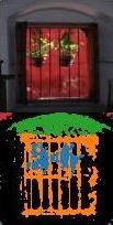
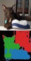
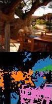
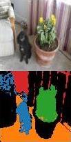
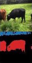
Figure 3: Visualizations of bottom-up grouping by CLIPpy. Each color represents one grouping learned on a given image.

4.2 Emergence of Bottom-Up Perceptual Grouping

Unsupervised segmentation performance is a direct measure of bottom up perceptual grouping. We apply CLIPpy at test time to perform semantic segmentation without prompting it for any labels . Fig. 3 shows how the model visually groups semantically related regions of an image (see also Fig. 5 in App.) as the image embeddings naturally group into spatially distinct clusters mirroring the image structure. We emphasize that this analysis does not rely on text prompts nor segmentation labels, but merely emerges from the image features alone. Hence the model has learned to group perceptually related pixels merely based on the pixel content and associated image-level captions during training.

We quantify the accuracy of this bottom-up segmentation to capture known segmentations within annotated images. Following evaluation protocol in [12, 113], we compute the Jaccard Similarity (JS). JS here measures the average intersection over the union across all segmentation instances regardless of object category. Our results in Tabs. 3, 5 and 4 demonstrate competitive performance by CLIPpy. In VOC, CLIPpy achieves $54.6\%$ outperforming all previous models; in comparison, CLIP achieves 38.9%. Additionally, on two more challenging datasets we note how the model drops in performance relatively, perhaps indicative of more visually cluttered scenes (Tab. 4). Our intuition for CLIPpy improving over CLIP is that CLS and average pooling breaks spatial structure of features, mixing image-level features across features at all spatial locations. We take these results to indicate that CLIPpy perceptually groups semantically related content better than previous work, providing state-of-the-art results in unsupervised segmentation.

	Dataset	Train	SSP	VOC
DeiT [12]	ImageNet	class	✗	24.6
MoCo [113]		self	✓	28.2
DINO [12]		self	✓	45.9
DSM [73]		self	✓	37.2
COMUS [119]		self	✓	47.3
DINO [113]	CC-12M & YFCC-100M	self	✓	41.8
CLIP [113]		text	✗	28.6
GroupViT [113]		text	✗	51.8
CLIP †	CC-12M	text	✗	37.3
GroupViT †		text	✓	42.8 ${}_{\text{{\color[rgb]{0,0.88,0}(+5.5)}}}$
CLIPpy		text	✓	47.5 ${}_{\text{{\color[rgb]{0,0.88,0}(+10.2)}}}$
CLIP †	HQITP-134M	text	✗	38.9
CLIPpy		text	✓	54.6 ${}_{\text{{\color[rgb]{0,0.88,0}(+15.7)}}}$

Table 3: CLIPpy effectively performs bottom-up grouping. We report Jaccard Similarity, an instance average of IoU between predicted and annotated segmentations, independent of object labels. ^†denotes our implementations. SSP indicates the use of self-supervised visual pre-training.

	Dataset	ADE20K	COCO
CLIP †	CC-12M	22.9	20.4
CLIPpy		28.9 ${}_{\text{{\color[rgb]{0,0.88,0}(+6.0)}}}$	26.0 ${}_{\text{{\color[rgb]{0,0.88,0}(+5.6)}}}$
CLIP †	HQITP-134M	24.2	21.6
CLIPpy		29.5 ${}_{\text{{\color[rgb]{0,0.88,0}(+5.3)}}}$	27.2 ${}_{\text{{\color[rgb]{0,0.88,0}(+5.6)}}}$

Table 4: More bottom-up grouping: CLIPpy improves Jaccard Similarity across datasets.

Method	JS
IIC [49]	6.4
MDC [11]	7.1
PiCIE [18]	12.3
STEGO [41]	21.0
CLIPpy (ours)	22.3

Table 5: More bottom-up grouping: CLIPpy achieves competitive Jaccard Similarity (JS) on the Cityscapes Dataset 27 class segmentation setup [41].

	Arch	Dataset	SSP	ADE20K	COCO	VOC	COCO (obj)
GroupViT [113]	ViT	CC-12M	✗	-	-	41.1	-
GroupViT †	ViT		✓	6.2	12.7	40.1	17.5
MaskCLIP † [126]	ViT		✗	6.8	8.1	22.1	13.8
OVS [114]	ViT		✓	7.1	-	44.6	25.1
CLIP †	ViT		✗	5.0	7.8	17.5	13.2
CLIPpy	ViT		✓	13.1 ${}_{\text{{\color[rgb]{0,0.88,0}(+8.1)}}}$	23.8 ${}_{\text{{\color[rgb]{0,0.88,0}(+16.0)}}}$	50.8 ${}_{\text{{\color[rgb]{0,0.88,0}(+33.3)}}}$	28.5 ${}_{\text{{\color[rgb]{0,0.88,0}(+15.3)}}}$
ALIGN [35]	CNN	ALIGN-1800M	✗	9.7	15.6	-	-
CLIP [85]	ViT	CLIP-400M	✗	5.8	8.7	16.4	14.5
ALIGN †	CNN	HQITP-134M	✗	7.5	14.4	29.7	-
CLIP †	ViT		✗	5.1	8.0	18.1	14.5
CLIPpy	ViT		✓	13.5 ${}_{\text{{\color[rgb]{0,0.88,0}(+8.4)}}}$	25.5 ${}_{\text{{\color[rgb]{0,0.88,0}(+17.5)}}}$	52.2 ${}_{\text{{\color[rgb]{0,0.88,0}(+34.1)}}}$	32.0 ${}_{\text{{\color[rgb]{0,0.88,0}(+17.5)}}}$

Table 6: CLIPpy provides competitive localization with no segmentation or location annotations. All models trained without any segmentation annotations. Results grouped by training dataset (bold highlights best per dataset). Numbers are mean IoU. ^† indicates our implementation. SSP indicates image self-supervised pre-training to visual encoder.

4.3 Top-down Grouping

We demonstrated that CLIPpy is able to perceptually group visual content within an image. Next, we ask how well this grouping corresponds to semantically meaningful labels. To measure the emergence of top-down grouping, we ask how well the perceptual grouping of the model may be steered by embeddings from the language model. We test this by comparing the model’s ability to perform zero-shot semantic segmentation across four datasets. Note that all of our results and comparisons are solely restricted to models trained on no segmentation annotations.

Fig. 1 provides a visualization of the predicted zero-shot segmentations (see also App. B), and Tab. 6 quantifies the results using mean intersection over union (mIoU). CLIPpy outperforms all other approaches on semantic segmentation when trained on the same datasets, both for CC-12M and HQITP-134M. We view our datasets in two categories: ADE20K and COCO contain numerous background classes while VOC and COCO (obj) contain only foreground object classes. We particularly highlight the notable performance improvement of CLIPpy for the former datasets. Moreover, in comparison to CLIP and ALIGN baselines, CLIPpy achieves significant improvements. We also replicate these baselines on the largest possible dataset within our compute budget (HQITP), for comparison on a common dataset. These results on HQITP also indicate clear performance improvements from CLIPpy.

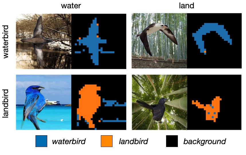
CLIP	water	land	$\Delta$
waterbird	80.2	48.1	-32.1
landbird	38.8	71.7	-32.9

CLIPpy	water	land	$\Delta$
waterbird	76.9	74.9	-2.0
landbird	80.0	84.1	-4.1

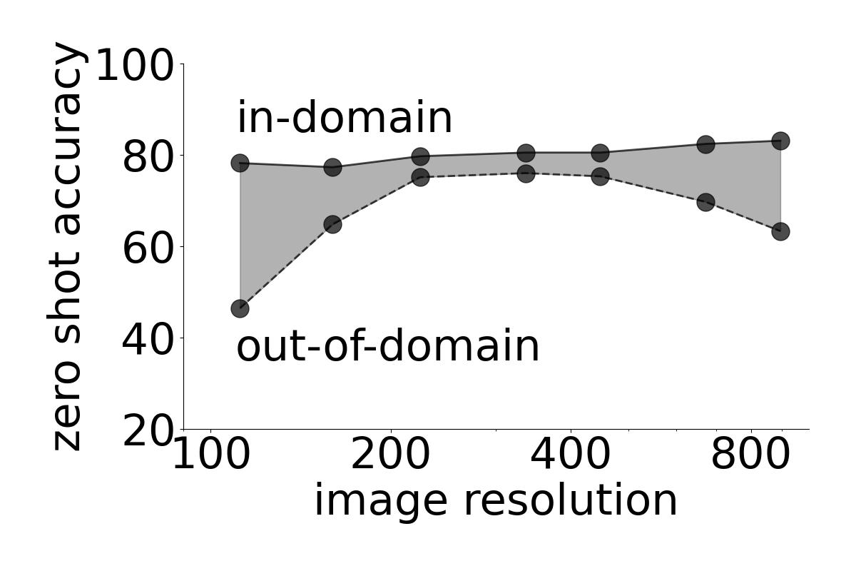
Figure 4: Perceptual grouping mitigates sensitivity to spurious correlations. (left) Selected segmentation examples by CLIPpy of waterbirds and landbirds on each background. (centre) Accuracy on the test split (5794 examples) of Waterbirds on CLIP and CLIPpy evaluated at 448$\times$448 resolution. The domain gap $\Delta$ reports the drop in accuracy between on and off diagonal entries within a row. (right) Zero shot accuracy of CLIPpy across image resolution for landbirds on land (top) and water (bottom). Note log axis. Shading highlights $\Delta$.

GroupViT [113] and OVS [114] provide important points of comparison. These models use custom ViT architectures specific to grouping, are trained on common datasets (containing image-text pairs), and are designed to perform perceptual grouping by optimizing discretized attention masks. We draw attention to the clear performance improvements of CLIPpy over these methods across all datasets. We also highlight that OVS [114] uses pre-training strategies similar to ours. Our implementation of GroupViT also utilizes similar pre-training following [114]. We take these results to mean that our simple changes to existing vision-language models uncover powerful localization information.

4.4 Perceptual grouping may improve robustness

We have observed how parsimonious changes to vision-language models result in state-of-the-art unsupervised and zero-shot semantic segmentation. In this section, we ask how the resulting perceptual grouping may be exploited to improve the robustness of image understanding. A large literature has consistently observed that models systematically underperform under domain shifts [87]. For instance, CLIP, ALIGN, and CLIPpy underperform on ImageNet-v2 versus ImageNet (Tab. 2). Another means of assessing robustness is to measure how well a model causally predicts the label from the appropriate input variates [81, 82]. To probe for causal dependencies, one can measure model performance to counterfactual examples where an input is selectively manipulated in order to test for sensitivity to spurious correlations.

A common formulation for this problem is to artificially synthesize a malicious dataset where a trained model may correlate inappropriate image features to predict a label [112, 74, 46, 2]. A large class of supervised learning algorithms have been developed to train on these datasets with the aim of mitigating such spurious correlations [91, 65, 76]. One common synthetic benchmark is Waterbirds [91] which places segmentations of birds in front of a background of land or water. The goal of any prediction system is a two-way classification of whether or not a bird is from the waterbird or landbird category. What makes this problem particularly challenging is when the background is not commensurate with the type of bird. For instance, a trained model may be prone to predict the type of bird due to the presence of water in the background in lieu of the visual appearance of the actual bird.

We first asked how our baseline CLIP model performs on this task when presented with a zero-shot three-way classification task (App. H for inference procedure). Model performance depends heavily on the background (Fig. 4 centre). For instance, the prediction accuracy of waterbirds drops by $\Delta$=32.1% (80.2 $\rightarrow$ 48.1) in the presence of an incommensurate background. Clearly, the baseline CLIP model performs zero-shot prediction by relying on features from the background. We note that open-source CLIP [85] has similar trends (see App. Tab. 11).

We next asked how CLIPpy performs given that it exhibits a unique ability to discriminate the spatial locations of objects. Fig. 4 shows selected examples from each class colored by the prediction at each spatial location. Clearly, the model is able to discriminate which locations correspond to each category. We quantify model accuracy across each task, and find the model far less sensitive to the background. For instance, in the case of waterbirds, CLIPpy accuracy, while slightly less than the baseline CLIP model, only drops by $\Delta$ = 2.0% (76.9 $\rightarrow$ 74.9) in spite of the background change (Fig. 4 right). Interestingly, the domain gap $\Delta$ is minimal ($\sim$4%) around a broad range of image input resolutions centered about the training resolution of the model (Fig. 4). Hence, CLIPpy, while still susceptible to some spurious correlations, is far more robust than a standard vision-language model.

As points of comparison, all prior work train a supervised model on the training split. In contrast, our predictions are zero-shot, and we do not use the training set. This difference makes a direct comparison of the raw accuracy difficult. That said, the best supervised training methods achieve a domain gap $\Delta$ of 4% to 8% (Tab. 1 and priv. correspondence, [65]), comparable to our results. We take these results to indicate that our zero-shot approach leveraging perceptual grouping provides another approach for addressing spurious correlations and learning robust image features.

4.5 Ablation Studies

We next perform experiments to demonstrate how individual factors in CLIPpy led to improved localization.

We first explore the effect of pre-trained representations. In Tab. 7, we freeze each of the backbones with self-supervised pre-training [12] for the image backbone and sentence T5 pre-training [78] for the text backbone. Our ablations indicate that the pre-trained weights alone do not contribute to the strong perceptual grouping of CLIPpy: our modified training process is necessary. In fact, both classification and semantic segmentation performance is affected negatively by freezing either backbone.

We also explore how alternate or no pre-training effects overall performance. Table 8 explores the selective removal of pre-training on the image model, language model or both. All models employ maximum pooling aggregation across spatial locations. Again, we see that CLIPpy exhibits significant drops in both zero-shot image recognition and localization by selectively dropping out each pre-training step. For instance, model performance drops from 42.3% to 25.6% top-1 accuracy. Likewise, the semantic segmentation mIoU drops from 50.8% to 23.5% accuracy. As expected, ImageNet supervised pre-training improves ImageNet top-1 accuracy, but interestingly leads to significant drops in grouping performance. For bottom-up segmentation, initializing from pretrained models benefits from scaling up the joint training data (Tab. 8 vs. 13). We suspect that these results indicate how each initialization provides valuable prior information not readily available in joint training for eliciting strong grouping properties, while also demonstrating the need for our training mechanism to emerge such grouping behaviour.

Aggregation	I-F	T-F	IN (Acc)	VOC (mIoU)
Cls	✓	✗	39.9	3.4
Max	✓	✗	24.2	10.4
Max	✗	✓	35.9	29.5
Max	✗	✗	42.3	50.8

Table 7: Ablation on freezing pre-trained backbones: We report Top-1 accuracy (%) for ImageNet (IN) and mean IoU for VOC. I-P stands for image backbone pooling, I-F stands for image backbone frozen, and T-F stands for text backbone frozen.

Dataset	Image	T5	ImageNet	Pascal VOC
	Init	Init?	Accuracy	mIoU	Jaccard
CC-12M	DINO	✓	42.3	50.8	47.5
	IN-1K	✓	53.3	22.5	43.3
	random	✓	28.9	32.9	43.6
	DINO		34.1	44.3	47.2
	IN-1K		44.5	20.0	42.2
	random		25.6	23.5	43.1

Table 8: Ablation on alternate pre-training: We report Top-1 accuracy (%) for ImageNet and mean IoU & Jaccard Similarity for VOC. Image encoder is initialized with DINO, supervised training on ImageNet-1K, or random weights. Text encoder is initialized with Sentence T5 or random weights. Parallel ablations using HQITP-134M in App. A.3.

We next ablate the choice of aggregation mechanism. CLIPpy employs a maximum operation over all spatial locations. We likewise train models performing spatial averaging or employing a class token. We present these results in Tab. 9. The standard procedures of class token and average pooling result in similar performance on zero-shot classification on ImageNet, but notable reductions in mIoU on VOC semantic segmentation. For instance, in the model trained with CC-12M, mIoU on VOC drops from 50.8% to 4.0% representing a relative drop of 91.3%. Similarly, in the case of bottom-up grouping on the same dataset, we demonstrate a 10 point drop in JS. We use these results to highlight the significant role played by the aggregation mechanism in inducing observed grouping properties.

We finally explore the effect of proposed token sub-sampling in Tab. 10. Improvements in classification and semantic segmentation performance across datasets verify its role in boosting performance.

Dataset	Aggreg.	ImageNet	Pascal VOC
		Accuracy	mIoU	Jaccard
CC-12M	Max	42.3	50.8	47.5
	Avg	44.0	11.6	38.1
	Cls	46.0	4.0	40.4
HQITP-134M	Max	59.0	50.1	54.6
	Avg	60.0	17.9	40.5
	Cls	60.2	4.1	41.3

Table 9: Ablation across aggregation methods: We report Top-1 accuracy (%) for ImageNet and mean IoU & Jaccard Similarity for VOC. Global max pooling (Max), global average pooling (Avg), and class token (Cls) alternatives are explored. All models initialized with the same pre-trained features.

TSS	IN	VOC	COCO	ADE20K
✗	45.3	50.9	23.5	12.6
✓	45.6	51.8	24.1	13.4

Table 10: Ablation on token sub-sampling: We report top-1 accuracy (%) for ImageNet (IN) and mean IoU for the three segmentation datasets (VOC, COCO, ADE20K). TSS stands for token sub-sampling.

5 Discussion

In this work we demonstrated how contrastive vision-language models have a profound lack of understanding object location. We described a minimal set of changes to existing vision-language models by modifying the aggregation method, introducing optimal pre-training strategies, and train-time token sub-sampling techniques to endow the model with both bottom-up and top-down perceptual grouping. We emphasize that our changes are minimal but sufficient to match if not exceed the performance of custom-built architectures [113, 114] in achieving perceptual grouping. We demonstrate that our resulting model provides state-of-the-art results in terms of unsupervised segmentation, and competitive results in terms of zero-shot semantic segmentation – even though the model has been afforded no segmentation annotations whatsoever. Finally, we demonstrate the utility of these representations by demonstrating how perceptual grouping may be leveraged to learn visual features that are robust to spurious correlations.

We take these results to indicate that contrastive vision-language models may provide the emergence of perceptual grouping without supervision. We do see limitations in this approach as segmentation suffers with increasing visual clutter and label cardinality (e.g. ADE-20K). We suspect that recent advent of larger-scale open datasets [92, 10] and advances in self-supervised learning [41, 73] may offer opportunities to demonstrate further benefits for endowing models with perceptual grouping. We also note the possibility of biases in our training data that may be reflected in our models.

Reproducibility Statement

We built a codebase derived from OpenAI CLIP source code (https://github.com/openai). Source code changes to accommodate our modifications to architecture and training were minimal, and are all documented in Sec. 3. We employed pretrained Sentence T5 Base language models from HuggingFace (https://huggingface.co) and image models from [12, 27]. The CC-12M dataset was downloaded from [14] and provides a publicly reproducible benchmark. HQITP-134M can not be publicly released due to copyright issues. All reported numbers also contain an equivalent version for a model trained only on CC-12M to enable reproducibility.

Ethics Statement

We describe a minimal set of changes to vision-language models to endow these models with perceptual grouping and localization information. Our work contributes to a large literature for how to build more performant and generalizable vision models. We use both public and private computer vision datasets and leverage pretrained language and image models for our experiments. Although we believe our code and model architecture to contain no inherent bias, both the public and private data we employ may contain such biases. Any trained model should thus be approached and deployed with caution to ensure that that all fairness and bias issues are properly addressed.

Acknowledgments

We would like to thank the broader research team at Apple for support, feedback and guidance. In particular, we would like to thank Tom Gunter, Tom Nickson, Chen Chen, Floris Weers, Arjun Desai, Soroush Abbasi Koohpayegani, Dan Busbridge, Oncel Tuzel, Navdeep Jaitly, and Albin Madappally Jose for technical feedback and support; Samy Bengio, Barry Theobald, Russ Webb, Ayesha Rehman, and Marco Zuiliani for logistical help and encouragement throughout the project.

Appendix: Perceptual Grouping in Contrastive Vision-Language Models

Contributions

KR led the project by performing most of experiments, evaluations and visualizations. BM helped build the codebase, debugged many issues, worked on the evaluations, and discussed many of the pooling methods explored. SR ran early experiments on localization datasets to explore potential applications in transfer learning and detection. YY discussed all aspects of the project idea and scope, built and trained the initial CLIP implementation, and contributed many ideas to the pooling and initialization. AT advised on the project, proposed many pretraining and pooling experiments, analyzed results, contributed to writing and reviewed code. JS organized the project, set the research direction, discussed all aspects of the project idea and scope, and wrote much of the paper.

Appendix A Additional Quantitative Results

In this section, we present additional quantitative evaluations for better understanding our experimental outcomes. We first extend our robustness analysis, followed by additional ablations on aggregation and pretraining strategies.

A.1 Robustness Analysis

We explore the open-source CLIP model from [85], evaluating its performance on the waterbirds dataset for signs of spurious correlations learned by the model. These results presented in Tab. 11 illustrate how classification performance for the same set of foreground objects drops drastically against different conflicting backgrounds, even in spite of the task involving fine-grained categories of birds.

CLIP [85]	water	land	$\Delta$
waterbird	88.3	70.1	-18.2
landbird	90.5	99.1	-8.6

Table 11: Waterbirds evaluation for OpenAI CLIP model. We demonstrate how even a CLIP model trained on significantly more data (400M image-text pairs) contains stronger sensitivty to spurious correlations than CLIPpy trained with an order of magnitude less data (12M). The first two columns report top-1 classification accuracy (%) and the last column reports difference of diagonal and off-diagonal terms (delta). Higher spurious correlations increase the absolute value of delta.

A.2 Alternate Aggregation Strategies

Having explored two standard visual aggregation techniques as baselines, we ask how aggregation on the textual encoder affects CLIPpy performance. In detail, we first explore maximum pooling for the language modality. Thereafter, we draw further attention to the visual modality, exploring more complex pooling strategies.

Language Modality. In Tab. 12, we explore how pooling on the text embedding affects overall performance. We replace default average pooling with a maximum pooling operation to discover drops in performance across all metrics. This poor performance of maximum pooling based aggregation for language is consistent with prior works [42]. We hypothesize the reasoning as the nature of our task: while we attempt a localization across the visual modality, on the language end we reason with the entire text prompt as a single unit.

Visual Modality. We explored a range of alternate aggregation strategies that performed subpar to spatial max pooling utilized in CLIPpy. Two noteworthy approaches include Text Similarity Pooling (TSP) and Weighted Maximum Pooling (WMP). In TSP, we measure the similarity of each spatial token (corresponding to different positions) and obtain a normalized distribution using a softmax operation (including a temperature for smoothing). We aggregate the visual modality using a weighted averaging operation where the similarity of each spatial location to the text is the weight. WMP follows the same idea but employs per-channel per-location embedding values instead of similarity as weights for the aggregation operation. Tab. 14 shows results for TSP, WMP and max pooling. TSP performs poorly across all variations while WMP works better at lower temperatures. Given the common softmax operation, higher temperature values result in smoother weights for both cases, making WMP and TSP more similar to average pooling. In the case of WMP, lower temperatures make the operation similar to simple spatial maximum pooling, which is reflected in the improved results for lower temperature values.

Method	IN	VOC	COCO	ADE-20K
Avg	45.3	50.8	23.8	13.1
Max	42.0	42.6	18.9	10.5

Table 12: Alternate Pooling Strategies for Text Modality. Unlike the visual modality, performance drops when replacing the default average pooling (Avg) with maximum pooling (Max).

dataset	image	T5	ImageNet	Pascal VOC
	init	init?	accuracy	mIoU	Jaccard
HQITP -134M	DINO	✓	59.0	50.1	54.6
	IN-1K	✓	63.6	21.7	40.2
	random	✓	49.4	37.3	46.3
	DINO		55.2	46.9	53.7
	IN-1K		60.6	20.9	39.1
	random		46.4	37.1	45.8

Table 13: Additional ablation studies with HQITP-134M. Parallel results for Table 8 (center) for ablations on weight initialization. We observe similar trends in results across these experiments.

Method	temp	IN	VOC	COCO	ADE-20K
TSP	0.1	0	2.98	0	0
TSP	1.0	20.15	4.91	1.25	0
TSP	10	24.70	15.83	4.27	2.29
Max		27.05	37.39	17.32	9.69

Method	temp	IN	VOC	COCO	ADE-20K
WMP	0.1	28.36	31.12	13.64	8.12
WMP	1.0	0	0	0	0
WMP	10	0	3.53	0	0
Max		27.05	37.39	17.32	9.69

Table 14: Alternate Pooling Strategies for Visual Modality. We report results for TSP and WMP with models trained for lesser steps on CC-12M with no initialization. Max refers to the spatial max operation used in CLIPpy. The temperature of the softmax operation for TSP and WMP is indicated by temp.

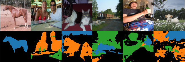
Figure 5: Qualitative examples of bottom-up unsupervised segmentation with CLIPpy. We illustrate examples from PASCAL VOC dataset with original image and CLIPpy prediction in the top and bottom rows, respectively. Note that colors correspond to clusters and not semantic labels.

A.3 Pretraining Ablations

Self-supervised pretraining of the vision head of CLIPpy leads to notable performance gains. We also explore how alternate supervised pretraining affects performance. In particular, we pretrain the image backbone using ImageNet-1K in a fully-supervised setting, and use the penultimate features to initialize CLIPpy. Apart from pretraining, all hyperparameters are unchanged. We present these results in Tab. 13. We observe when training with HQITP-134M that supervised pretraining leads to considerable performance gains for ImageNet-1K top-1 accuracy, but a considerable drop in segmentation performance across all three datasets. However, we note that supervised ImageNet pre-training provides unfair advantage in the case of ImageNet accuracy, in particular given the ability of overfitting those visual concepts. So we focus more on the segmentation results. Interestingly, entirely eliminating visual pre-training, while degrading segmentation performance, outperforms the ImageNet supervised pre-training initialized model. This reaffirms our hypothesis of better generalization of self-supervised features for segmentation tasks. We also note that results on HQITP-134M indicate trends similar to those with CC-12M.

Appendix B Qualitative examples of localization

In this section, we showcase additional qualitative examples of the success and failures of CLIPpy on bottom-up unsupervised segmentation and top-down semantic segmentation.

Fig. 5 shows examples of bottom-up unsupervised segmentation on PASCAL VOC for CLIPpy. The left three examples highlight the strength of the method for images with less clutter in which there is a single object of interest. The right three examples shows examples highlights the failures in the presence of scene clutter.

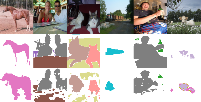
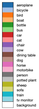
COCO

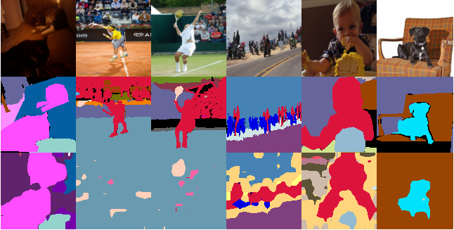
ADE-20K

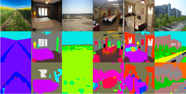
Figure 6: Qualitative examples of top-down semantic segmentation with CLIPpy from PASCAL VOC, COCO and ADE-20K. For Pascal VOC, we supply a color legend for the 20 label classes. Note that the Pascal VOC examples correspond to the same examples from Fig. 5.

Fig. 6 present additional top-down semantic segmentation examples across all three datasets used for evaluation. The examples from PASCAL VOC dataset are the same examples from Fig. 5. For PASCAL VOC, note that the contrast between the top-down and bottom-up segmentations. The top-down segmentation is able to correctly separate the dog and cat classes (column 3) and also improve performance in the more cluttered scenes. On the other hand, in column 4, it missed out on a portion of the train that was segmented properly in the bottom-up setting. Segmentations from CLIPpy may contain discontinuities within a single object region in some cases, especially for the background objects (columns 2-3).

COCO and ADE-20K provide more challenging datasets and highlight several potential failure modes. A notable failure mode for CLIPpy is to reverting to the baseline CLIP behaviour by predicting the salient object class at all locations. This is visible to some extent in column 2 & 3 in the COCO examples and column 3 in the ADE-20K examples. Additionally, CLIPpy results in false positives for cluttered scenes as visible in some examples of these two datasets.

In summary, CLIPpy is able to localize the salient objects well in less cluttered scenes, even when multiple objects belonging to different classes are present. CLIPpy is also able to coarsely localize some of the salient objects in more cluttered scenes. In terms of limitations, CLIPpy fails to correctly localize some background classes, fails to correctly recognize object boundaries, and may miss smaller objects in cluttered scenes.

Appendix C Details of HQITP-134M dataset

High Quality Image Text Pairs (HQITP-134M) consists of $\sim$134 million diverse and high quality images paired with descriptive captions and titles. Images range in spatial resolution from 320 to 2048 pixels on the short side. All images are JPEG format and most are RGB. Each example image is associated with a title, and a list of several captions. A small fraction (<< 1%) of the examples are missing both captions and title. We favor the associated captions, and find that these tokenize to an average length of 20.1 tokens, although the shortest caption is only one token and the longest is over 1000. This dataset was licensed to our research lab by a third party for commercial use.

To preprocess this dataset for training, we first exclude all pairs for which no valid caption exists. We also perform global exact-byte-match image de-duplication across our full training corpus, meaning that valid examples may be dropped due to appearing in other subsets of our overall training dataset. As we draw each example, we create an image-text pair by sampling from the list of available captions. The text is then tokenized, and the image is resized so that the shortest side is 224 pixels, with a further random crop then applied over the longer dimension to produce a 224 x 224 pixel square image. Lastly, we normalize the image using statistics derived from our full training corpus.

Appendix D Architecture and Training Details

Our implementations of CLIP and ALIGN employ ViT-B/16 [27], and EfficientNet-B5[100] for the image embedding, respectively, to mirror the primary results presented in each respective vision-language model. For the ViT architecture, we experimented with varying patch sizes $P=8$ and $P=16$ in order to leverage open-sourced DINO pretrained weights [12], but report all of our results with $P=16$.

We train all models on 224$\times$224 images to provide a fair comparison with [85]. Note however that the published version of ALIGN employed a 640$\times$640 resolution. ViT models may operate on images at arbitrary spatial resolution. At inference time we experimented with spatial resolutions of 224$\times$224 and 448$\times$448, resulting in 196 and 784 tokens, respectively. Results were similar across 224 and 448 resolutions, we report only results at 224 for brevity (except for Fig. 4).

We train models with 32 GPUs across 4 machines with PyTorch [80] using the LAMB optimizer [116] with a cosine decayed learning rate with linear warm-up. We employ an initial learning rate of 1e-3, 2000 warm-up steps, and decay the rate with a single period over the entire training regime (32 epochs for CC12M; 10 epochs for HQITP-134M). We employ a weight decay of 1e-2. All training parameters were determined through moderate hyperparameter tuning.

Patch Sub-Sampling: During training, we also utilize overlapping patch generation with patch sub-sampling as regularization. In particular, the token sequence length is always maintained at the original value of 224 during training through random sub-sampling (patches selected according to uniform distribution). This also allows obtaining a higher resolution feature map from a fixed resolution image during inference.

Appendix E Limitations of CNN-based architectures

The primary focus of our presentation is on the Vision Transformer (ViT) architecture [27]. The reason for this focus is that the Transformer architecture is particularly well suited for multimodal learning tasks because one does not need to craft an architecture for each modality, and tune the training set up for each particular architecture. We also recognize that convolutional neural networks (CNN’s) have a long history of providing state-of-the-art CNN results on computer vision related problems. EfficientNet-B5 is a modern state-of-the-art architecture whose meta-architecture and scaling properties were derived from architecture search considerations [100] (but see [5]), and provides the visual backbone for the ALIGN model [50].

We experimented with this model and find that the image featurization from a CNN-derived backbone achieves favorable results with respect to previously published ViT models on localization problems. Table 6 showcases higher mIoU for semantic segmentation than a model with a ViT backbone (CLIP) on ADE20K, COCO and Pascal VOC when trained on the same dataset. Likewise, previous results published on ALIGN with an EfficientNet-B5 backbone achieved superior results to a ViT model on COCO and ADE20K in terms of semantic segmentation .

Most importantly, in spite of many attempts, we were not able to improve the performance of the EfficientNet-B5 architecture for localization. The best results for a CNN-based architecture we achieved are shown in Table 6, which are notably below previously published results and our best results with a ViT architecture. At best, the addition of maximum pooling at the top layer of a CNN led to marginal gains in terms of mIoU or Jaccard similarity. We suspect that a custom architecture (such as ASPP or FPN) may improve these results further [16, 63], but we consider this out of scope as we are attempting to learn a featurization that does not artificially increase the parameterization in order to solve a specialized task of localization. We suspect that this limitation of CNN architectures may reflect the fact that CNN architecture already have learned a representation that is heavily dependent on the spatial geometry derived from a convolutional kernel. Such an inductive bias may be not provide a suitable mechanism for providing global processing in a segmentation task [107].

	segment	segment
	label?	mask?	ADE20K	COCO	PASCAL VOC
SPNet [111]	✓	✓			18.3
ZS3Net [8]	✓	✓			38.3
LSeg [57]	✓	✓		27.2	47.4
LSeg+ [35]	✓	✓	18.0	55.1 †	59.0
ALIGN w/ proposal [35]		✓	12.9	17.9 †	22.4
OpenSeg [35]		✓	21.1	36.1 †	70.2
OpenSeg + Narr. [35]		✓	24.8	38.1 †	72.2

Table 15: Performance of prior zero-shot segmentation models trained on segmentation data. All numbers report the mIoU for semantic segmentation on ADE20K (150 labels), PASCAL-VOC (20 labels) and COCO (50 labels). $\dagger$ indicates models that were trained on image segmentation masks from the COCO dataset.

Appendix F Prior work on zero shot semantic segmentation

Recent work has made impressive strides on zero-shot semantic segmentation. These works focus on training such models on subsets of segmentation data, whether masks and/or labels and test the performance of the resulting model on other splits of data. The zero-shot performance is assessed by splitting the labeled datasets to ensure that the model is tested in a zero-shot manner on unseen labels. Table 15 summarizes results from several recent papers [36, 57, 111, 8]

We note that particularly later forms of models achieve results superior to those presented here [36, 57], but we emphasize several important distinctions. First, these models were trained on segmentation masks in order to learn perceptual grouping across visual imagery. Our work instead addresses how a model may learn this information without being explicitly supplied examples teaching such behavior. Second, most of the models were trained using segmentation masks from the COCO dataset. Hence, these models might perform particularly well on this dataset making comparisons on COCO less comparable to our model.

Appendix G Prior work on unsupervised segmentation

The task of unsupervised segmentation groups semantically related concepts using only pixel information. Recent advances in self-supervised learning (e.g. [12]) has led to numerous opportunities across tasks [61, 94], including for unsupervised segmentation or weakly-supervised localization tasks [41, 18, 31, 49, 93]. These methods train and operate with no semantic labels, performing bottom-up grouping of image content. A common characteristic is the presence of iterative clustering mechanisms (e.g. $k$-Means clustering [69]). Notably, STEGO [41] employs $k$-Means and Conditional Random Fields (CRF) [56] to refine and improve the inference procedure. We hope to apply CRFs (e.g. [47]) to CLIPpy in future. While CLIPpy exhibits competitive performance, we note that techniques proposed by other methods (e.g. [41]) may be leveraged (and combined with CLIPpy) to refine our segmentation performance. A key distinction of our work is the focus on learning a new representation space aligned to language that exhibits strong perceptual grouping.

Appendix H Details of robustness analysis

We calculate the zero-shot prediction of the class in a non-standard manner to exploit the spatial reasoning of CLIPpy. We apply the same zero-shot evaluation to the baseline CLIP model. Specifically, we first calculate the embedding for all labels within each category of waterbird, landbird and background. For each of these categories we calculate the average image embeddings across these labels at each spatial location.

To exploit the spatial knowledge of the model, we focus our analysis on all spatial locations which are not labeled as background. For all locations which maximally predict a waterbird, we calculate the similarity to the embedding for a waterbird. Likewise, we do the same for all locations maximized by landbird. Finally, our resulting prediction is the class that is closest to its associated embedding.

We find that these results and the corresponding robustness vary substantially due to the selection of prompts for each of the three categories. This matches observations in [85]. In Sec. 4.4 we focus on the results of the model trained on CC-12M using the prompts listed below which contain a minimal amount of prompt engineering. In particular, the prompts for waterbirds and landbirds follow [91]. See also [108].

• background: background

• waterbird: Black footed Albatross, Laysan Albatross, Sooty Albatross, Crested Auklet, Least Auklet, Parakeet Auklet, Rhinoceros Auklet, Brandt Cormorant, Red faced Cormorant, Pelagic Cormorant, Frigatebird, Northern Fulmar, Gadwall, Eared Grebe, Horned Grebe, Pied billed Grebe, Western Grebe, Pigeon Guillemot, California Gull, Glaucous winged Gull, Heermann Gull, Herring Gull, Ivory Gull, Ring billed Gull, Slaty backed Gull, Western Gull, Long tailed Jaeger, Pomarine Jaeger, Red legged Kittiwake, Pacific Loon, Mallard, Hooded Merganser, Red breasted Merganser, Brown Pelican, White Pelican, Horned Puffin, Artic Tern, Black Tern, Caspian Tern, Common Tern, Elegant Tern, Forsters Tern, Least Tern

• landbird: Groove billed Ani, Brewer Blackbird, Red winged Blackbird, Rusty Blackbird, Yellow headed Blackbird, Bobolink, Indigo Bunting, Lazuli Bunting, Painted Bunting, Cardinal, Spotted Catbird, Gray Catbird, Yellow breasted Chat, Eastern Towhee, Chuck will Widow, Bronzed Cowbird, Shiny Cowbird, Brown Creeper, American Crow, Fish Crow, Black billed Cuckoo, Mangrove Cuckoo, Yellow billed Cuckoo, Gray crowned Rosy Finch, Purple Finch, Northern Flicker, Acadian Flycatcher, Great Crested Flycatcher, Least Flycatcher, Olive sided Flycatcher, Scissor tailed Flycatcher, Vermilion Flycatcher, Yellow bellied Flycatcher, American Goldfinch, European Goldfinch, Boat tailed Grackle, Blue Grosbeak, Evening Grosbeak, Pine Grosbeak, Rose breasted Grosbeak, Anna Hummingbird, Ruby throated Hummingbird, Rufous Hummingbird, Green Violetear, Blue Jay, Florida Jay, Green Jay, Dark eyed Junco, Tropical Kingbird, Gray Kingbird, Belted Kingfisher, Green Kingfisher, Pied Kingfisher, Ringed Kingfisher, White breasted Kingfisher, Horned Lark, Western Meadowlark, Mockingbird, Nighthawk, Clark Nutcracker, White breasted Nuthatch, Baltimore Oriole, Hooded Oriole, Orchard Oriole, Scott Oriole, Ovenbird, Western Wood Pewee, Sayornis, American Pipit, Whip poor Will, Common Raven, White necked Raven, American Redstart, Geococcyx, Loggerhead Shrike, Great Grey Shrike, Baird Sparrow, Black throated Sparrow, Brewer Sparrow, Chipping Sparrow, Clay colored Sparrow, House Sparrow, Field Sparrow, Fox Sparrow, Grasshopper Sparrow, Harris Sparrow, Henslow Sparrow, Le Conte Sparrow, Lincoln Sparrow, Nelson Sharp tailed Sparrow, Savannah Sparrow, Seaside Sparrow, Song Sparrow, Tree Sparrow, Vesper Sparrow, White crowned Sparrow, White throated Sparrow, Cape Glossy Starling, Bank Swallow, Barn Swallow, Cliff Swallow, Tree Swallow, Scarlet Tanager, Summer Tanager, Green tailed Towhee, Brown Thrasher, Sage Thrasher, Black capped Vireo, Blue headed Vireo, Philadelphia Vireo, Red eyed Vireo, Warbling Vireo, White eyed Vireo, Yellow throated Vireo, Bay breasted Warbler, Black and white Warbler, Black throated Blue Warbler, Blue winged Warbler, Canada Warbler, Cape May Warbler, Cerulean Warbler, Chestnut sided Warbler, Golden winged Warbler, Hooded Warbler, Kentucky Warbler, Magnolia Warbler, Mourning Warbler, Myrtle Warbler, Nashville Warbler, Orange crowned Warbler, Palm Warbler, Pine Warbler, Prairie Warbler, Prothonotary Warbler, Swainson Warbler, Tennessee Warbler, Wilson Warbler, Worm eating Warbler, Yellow Warbler, Northern Waterthrush, Louisiana Waterthrush, Bohemian Waxwing, Cedar Waxwing, American Three toed Woodpecker, Pileated Woodpecker, Red bellied Woodpecker, Red cockaded Woodpecker, Red headed Woodpecker, Downy Woodpecker, Bewick Wren, Cactus Wren, Carolina Wren, House Wren, Marsh Wren, Rock Wren, Winter Wren, Common Yellowthroat

Appendix I Prompts for Zero-shot Segmentation

We employed the following prompts for probing our vision-language models for zero-shot semantic segmentation. These prompts were copied from the corresponding label sets of each dataset with some basic considerations, for instance, restoring spaces in compound words. For prompts separated by a comma, the average embedding across all prompts delineated by commas is associated with each label.

Pascal VOC 2012 [30]

1. background: background, crops, bush, shrub, tiles, pavement, rug, carpet, box, boxes, speaker, storage, painting, board, panel, poster, clock, cage, drinking glass, park, plaything, toy, fireplace, bag, bag, bed, bench, book, books, building, buildings, cabinet, drawer, ceiling, computer, computer case, cup, cups, door, fence, floor, flower, grass, lawn, turf, ground, soil, dirt, tiles, keyboard, lamp, mountain, hills, mouse, curtain, platform, sign, street, rock, stone, shelf, sidewalk, sky, clouds, snow, track, train track, tree, trees, wall, water, window, wood, woods

2. aeroplane: aeroplane, airplane, aeroplanes, airplanes

3. bicycle: bicycle, bicycles, bike, bikes

4. bird: bird, birds

5. boat: boat, boats

6. bottle: bottle, bottles, water bottle

7. bus: bus, buses

8. car: car, cars

9. cat: cat, cats, kitties, kitty

10. chair: chair, chairs

11. cow: cow, cows, calf

12. diningtable: diningtable, dining table, diningtables, dining tables, plate, plates

13. dog: dog, dogs, puppy, puppies

14. horse: horse, horses, foal

15. motorbike: motorbike, motorcycle, motorbikes, motorcycles

16. person: person, child, girl, boy, woman, man, people, children, girls, boys, women, men, lady, guy, ladies, guys, clothes

17. pottedplant: pottedplant, pottedplants, plant pot, plant pots, planter, planters, potted plant

18. sheep: sheep

19. sofa: sofa, sofas

20. train: train, trains, locomotive, locomotives, freight train

21. tvmonitor: tvmonitor, monitor, tv, televison, television monitor

COCO 2017 [64]

1. airplane: airplane

2. apple: apple

3. backpack: backpack

4. banana: banana

5. baseball bat: baseball bat

6. baseball glove: baseball glove

7. bear: bear

8. bed: bed

9. bench: bench

10. bicycle: bicycle

11. bird: bird

12. boat: boat

13. book: book

14. bottle: bottle

15. bowl: bowl

16. broccoli: broccoli

17. bus: bus

18. cake: cake

19. car: car

20. carrot: carrot

21. cat: cat

22. cell phone: cell phone

23. chair: chair

24. clock: clock

25. couch: couch

26. cow: cow

27. cup: cup

28. dining table: dining table

29. dog: dog

30. donut: donut

31. elephant: elephant

32. fire hydrant: fire hydrant

33. fork: fork

34. frisbee: frisbee

35. giraffe: giraffe

36. hair drier: hair drier

37. handbag: handbag

38. horse: horse

39. hot dog: hot dog

40. keyboard: keyboard

41. kite: kite

42. knife: knife

43. laptop: laptop

44. microwave: microwave

45. motorcycle: motorcycle

46. mouse: mouse

47. orange: orange

48. oven: oven

49. parking meter: parking meter

50. person: person

51. pizza: pizza

52. potted plant: potted plant

53. refrigerator: refrigerator

54. remote: remote

55. sandwich: sandwich

56. scissors: scissors

57. sheep: sheep

58. sink: sink

59. skateboard: skateboard

60. skis: skis

61. snowboard: snowboard

62. spoon: spoon

63. sports ball: sports ball

64. stop sign: stop sign

65. suitcase: suitcase

66. surfboard: surfboard

67. teddy bear: teddy bear

68. tennis racket: tennis racket

69. tie: tie

70. toaster: toaster

71. toilet: toilet

72. toothbrush: toothbrush

73. traffic light: traffic light

74. train: train

75. truck: truck

76. tv: tv

77. umbrella: umbrella

78. vase: vase

79. wine glass: wine glass

80. zebra: zebra

ADE-20K (150 frequent labels) [125]

1. airplane: airplane, aeroplane, plane

2. animal: animal, animate, being, beast, brute, creature, fauna

3. apparel: apparel, wearing, apparel, dress, clothes

4. arcade: arcade, machine

5. armchair: armchair

6. ashcan: ashcan, trash, can, garbage, can, wastebin, ash, bin, ash-bin, ashbin, dustbin, trash, barrel, trash, bin

7. awning: awning, sunshade, sunblind

8. bag: bag

9. ball: ball

10. bannister: bannister, banister, balustrade, balusters, handrail

11. bar: bar

12. barrel: barrel, cask

13. base: base, pedestal, stand

14. basket: basket, handbasket

15. bathtub: bathtub, bathing, tub, bath, tub

16. bed: bed

17. bench: bench

18. bicycle: bicycle, bike, wheel, cycle

19. blanket: blanket, cover

20. blind: blind, screen

21. boat: boat

22. book: book

23. bookcase: bookcase

24. booth: booth, cubicle, stall, kiosk

25. bottle: bottle

26. box: box

27. bridge: bridge, span

28. buffet: buffet, counter, sideboard

29. building: building, edifice

30. bulletin: bulletin, board, notice, board

31. bus: bus, autobus, coach, charabanc, double-decker, jitney, motorbus, motorcoach, omnibus, passenger, vehicle

32. cabinet: cabinet

33. canopy: canopy

34. car: car, auto, automobile, machine, motorcar

35. case: case, display, case, showcase, vitrine

36. ceiling: ceiling

37. chair: chair

38. chandelier: chandelier, pendant, pendent

39. chest: chest of drawers, chest, bureau, dresser

40. clock: clock

41. coffee: coffee, table, cocktail, table

42. column: column, pillar

43. computer: computer, computing, machine, computing, device, data, processor, electronic, computer, information, processing, system

44. conveyer: conveyer, belt, conveyor, belt, conveyer, conveyor, transporter

45. counter: counter

46. countertop: countertop

47. cradle: cradle

48. crt: crt, screen

49. curtain: curtain, drape, drapery, mantle, pall

50. cushion: cushion

51. desk: desk

52. dirt: dirt, track

53. dishwasher: dishwasher, dish, washer, dishwashing, machine

54. door: door, double, door

55. earth: earth, ground

56. escalator: escalator, moving, staircase, moving, stairway

57. fan: fan

58. fence: fence, fencing

59. field: field

60. fireplace: fireplace, hearth, open, fireplace

61. flag: flag

62. floor: floor, flooring

63. flower: flower

64. food: food, solid, food

65. fountain: fountain

66. glass: glass, drinking, glass

67. grandstand: grandstand, covered, stand

68. grass: grass

69. hill: hill

70. hood: hood, exhaust, hood

71. house: house

72. hovel: hovel, hut, hutch, shack, shanty

73. kitchen: kitchen, island

74. lake: lake

75. lamp: lamp

76. land: land, ground, soil

77. light: light, light, source

78. microwave: microwave, microwave, oven

79. minibike: minibike, motorbike

80. mirror: mirror

81. monitor: monitor, monitoring, device

82. mountain: mountain, mount

83. ottoman: ottoman, pouf, pouffe, puff, hassock

84. oven: oven

85. painting: painting, picture

86. palm: palm, palm, tree

87. path: path

88. person: person, individual, someone, somebody, mortal, soul

89. pier: pier, wharf, wharfage, dock

90. pillow: pillow

91. plant: plant, flora, plant, life

92. plate: plate

93. plaything: plaything, toy

94. pole: pole

95. pool: pool, table, billiard, table, snooker, table

96. poster: poster, posting, placard, notice, bill, card

97. pot: pot, flowerpot

98. radiator: radiator

99. railing: railing, rail

100. refrigerator: refrigerator, icebox

101. river: river

102. road: road, route

103. rock: rock, stone

104. rug: rug, carpet, carpeting

105. runway: runway

106. sand: sand

107. sconce: sconce

108. screen: screen, door, screen

109. screen: screen, silver, screen, projection, screen

110. sculpture: sculpture

111. sea: sea

112. seat: seat

113. shelf: shelf

114. ship: ship

115. shower: shower

116. sidewalk: sidewalk, pavement

117. signboard: signboard, sign

118. sink: sink

119. sky: sky

120. skyscraper: skyscraper

121. sofa: sofa, couch, lounge

122. stage: stage

123. stairs: stairs, steps

124. stairway: stairway, staircase

125. step: step, stair

126. stool: stool

127. stove: stove, kitchen, stove, range, kitchen, range, cooking, stove

128. streetlight: streetlight, street, lamp

129. swimming: swimming, pool, swimming, bath, natatorium

130. swivel: swivel, chair

131. table: table

132. tank: tank, storage, tank

133. television: television, television, receiver, television, set, tv, tv, set, idiot, box, boob, tube, telly, goggle, box

134. tent: tent, collapsible, shelter

135. toilet: toilet, can, commode, crapper, pot, potty, stool, throne

136. towel: towel

137. tower: tower

138. trade: trade, name, brand, name, brand, marque

139. traffic: traffic, light, traffic, signal, stoplight

140. tray: tray

141. tree: tree

142. truck: truck, motortruck

143. van: van

144. vase: vase

145. wall: wall

146. wardrobe: wardrobe, closet, press

147. washer: washer, automatic, washer, washing, machine

148. water: water

149. waterfall: waterfall, falls

150. windowpane: windowpane, window

Pascal VOC 2012

References

- [1] Pablo Arbeláez, Bharath Hariharan, Chunhui Gu, Saurabh Gupta, Lubomir Bourdev, and Jitendra Malik. Semantic segmentation using regions and parts. In CVPR, pages 3378–3385. IEEE, 2012.
- [2] Martin Arjovsky, Léon Bottou, Ishaan Gulrajani, and David Lopez-Paz. Invariant risk minimization. arXiv preprint arXiv:1907.02893, 2019.
- [3] Donghyeon Baek, Youngmin Oh, and Bumsub Ham. Exploiting a joint embedding space for generalized zero-shot semantic segmentation. In ICCV, 2021.
- [4] Zhipeng Bao, Pavel Tokmakov, A. Jabri, Yu-Xiong Wang, Adrien Gaidon, and Martial Hebert. Discovering objects that can move. 2022 IEEE/CVF Conference on Computer Vision and Pattern Recognition (CVPR), pages 11779–11788, 2022.
- [5] Irwan Bello, William Fedus, Xianzhi Du, Ekin Dogus Cubuk, Aravind Srinivas, Tsung-Yi Lin, Jonathon Shlens, and Barret Zoph. Revisiting resnets: Improved training and scaling strategies. NeurIPS, 34:22614–22627, 2021.
- [6] Samuel R Bowman, Gabor Angeli, Christopher Potts, and Christopher D Manning. A large annotated corpus for learning natural language inference. arXiv preprint arXiv:1508.05326, 2015.
- [7] Tom B. Brown, Benjamin Mann, Nick Ryder, Melanie Subbiah, Jared Kaplan, Prafulla Dhariwal, Arvind Neelakantan, Pranav Shyam, Girish Sastry, Amanda Askell, Sandhini Agarwal, Ariel Herbert-Voss, Gretchen Krueger, T. J. Henighan, Rewon Child, Aditya Ramesh, Daniel M. Ziegler, Jeff Wu, Clemens Winter, Christopher Hesse, Mark Chen, Eric Sigler, Mateusz Litwin, Scott Gray, Benjamin Chess, Jack Clark, Christopher Berner, Sam McCandlish, Alec Radford, Ilya Sutskever, and Dario Amodei. Language models are few-shot learners. ArXiv, abs/2005.14165, 2020.
- [8] Maxime Bucher, Tuan-Hung Vu, Matthieu Cord, and Patrick Pérez. Zero-shot semantic segmentation. NeurIPS, 2019.
- [9] Ryan Burgert, Kanchana Ranasinghe, Xiang Li, and Michael S. Ryoo. Peekaboo: Text to image diffusion models are zero-shot segmentors. ArXiv, abs/2211.13224, 2022.
- [10] Minwoo Byeon, Beomhee Park, Haecheon Kim, Sungjun Lee, Woonhyuk Baek, and Saehoon Kim. Coyo-700m: Image-text pair dataset. https://github.com/kakaobrain/coyo-dataset, 2022.
- [11] Mathilde Caron, Piotr Bojanowski, Armand Joulin, and Matthijs Douze. Deep clustering for unsupervised learning of visual features. In European Conference on Computer Vision, 2018.
- [12] Mathilde Caron, Hugo Touvron, Ishan Misra, Hervé Jégou, Julien Mairal, Piotr Bojanowski, and Armand Joulin. Emerging properties in self-supervised vision transformers. In CVPR, pages 9650–9660, 2021.
- [13] Junbum Cha, Jonghwan Mun, and Byung-Seok Roh. Learning to generate text-grounded mask for open-world semantic segmentation from only image-text pairs. ArXiv, abs/2212.00785, 2022.
- [14] Soravit Changpinyo, Piyush Sharma, Nan Ding, and Radu Soricut. Conceptual 12m: Pushing web-scale image-text pre-training to recognize long-tail visual concepts. In CVPR, pages 3558–3568, 2021.
- [15] Jiacheng Chen, Hexiang Hu, Hao Wu, Yuning Jiang, and Changhu Wang. Learning the best pooling strategy for visual semantic embedding. In CVPR, pages 15789–15798, 2021.
- [16] Liang-Chieh Chen, George Papandreou, Iasonas Kokkinos, Kevin Murphy, and Alan L Yuille. Deeplab: Semantic image segmentation with deep convolutional nets, atrous convolution, and fully connected crfs. IEEE TPAMI, 2017.
- [17] Bowen Cheng, Alexander G. Schwing, and Alexander Kirillov. Per-pixel classification is not all you need for semantic segmentation. arXiv, 2021.
- [18] Jang Hyun Cho, Utkarsh Mall, Kavita Bala, and Bharath Hariharan. Picie: Unsupervised semantic segmentation using invariance and equivariance in clustering. In Proceedings of the IEEE/CVF Conference on Computer Vision and Pattern Recognition, pages 16794–16804, 2021.
- [19] Dorin Comaniciu and Peter Meer. Robust analysis of feature spaces: Color image segmentation. In CVPR, pages 750–755. IEEE, 1997.
- [20] Marius Cordts, Mohamed Omran, Sebastian Ramos, Timo Rehfeld, Markus Enzweiler, Rodrigo Benenson, Uwe Franke, Stefan Roth, and Bernt Schiele. The cityscapes dataset for semantic urban scene understanding. 2016 IEEE Conference on Computer Vision and Pattern Recognition (CVPR), pages 3213–3223, 2016.
- [21] Elliot Creager, Jörn-Henrik Jacobsen, and Richard Zemel. Environment inference for invariant learning. In ICML, pages 2189–2200. PMLR, 2021.
- [22] Yufeng Cui, Lichen Zhao, Feng Liang, Yangguang Li, and Jing Shao. Democratizing contrastive language-image pre-training: A clip benchmark of data, model, and supervision. arXiv preprint arXiv:2203.05796, 2022.
- [23] Jia Deng, Wei Dong, Richard Socher, Li-Jia Li, Kai Li, and Li Fei-Fei. Imagenet: A large-scale hierarchical image database. In CVPR, pages 248–255. Ieee, 2009.
- [24] Karan Desai and Justin Johnson. Virtex: Learning visual representations from textual annotations. In CVPR, pages 11162–11173, 2021.
- [25] Jacob Devlin, Ming-Wei Chang, Kenton Lee, and Kristina Toutanova. Bert: Pre-training of deep bidirectional transformers for language understanding. arXiv preprint arXiv:1810.04805, 2018.
- [26] Jian Ding, Nan Xue, Guisong Xia, and Dengxin Dai. Decoupling zero-shot semantic segmentation. 2022 IEEE/CVF Conference on Computer Vision and Pattern Recognition (CVPR), pages 11573–11582, 2021.
- [27] Alexey Dosovitskiy, Lucas Beyer, Alexander Kolesnikov, Dirk Weissenborn, Xiaohua Zhai, Thomas Unterthiner, Mostafa Dehghani, Matthias Minderer, Georg Heigold, Sylvain Gelly, et al. An image is worth 16x16 words: Transformers for image recognition at scale. arXiv preprint arXiv:2010.11929, 2020.
- [28] Zi-Yi Dou, Aishwarya Kamath, Zhe Gan, Pengchuan Zhang, Jianfeng Wang, Linjie Li, Zicheng Liu, Ce Liu, Yann LeCun, Nanyun Peng, Jianfeng Gao, and Lijuan Wang. Coarse-to-fine vision-language pre-training with fusion in the backbone. ArXiv, abs/2206.07643, 2022.
- [29] Gamaleldin F. Elsayed, Aravindh Mahendran, Sjoerd van Steenkiste, Klaus Greff, Michael Curtis Mozer, and Thomas Kipf. Savi++: Towards end-to-end object-centric learning from real-world videos. ArXiv, abs/2206.07764, 2022.
- [30] Mark Everingham, Luc Van Gool, Christopher KI Williams, John Winn, and Andrew Zisserman. The pascal visual object classes (voc) challenge. IJCV, 2010.
- [31] Wouter Van Gansbeke, Simon Vandenhende, Stamatios Georgoulis, and Luc Van Gool. Unsupervised semantic segmentation by contrasting object mask proposals. ICCV, pages 10032–10042, 2021.
- [32] Tianyu Gao, Xingcheng Yao, and Danqi Chen. Simcse: Simple contrastive learning of sentence embeddings. arXiv preprint arXiv:2104.08821, 2021.
- [33] Andreas Geiger, Philip Lenz, and Raquel Urtasun. Are we ready for autonomous driving? the kitti vision benchmark suite. In CVPR, pages 3354–3361. IEEE, 2012.
- [34] Robert Geirhos, Kantharaju Narayanappa, Benjamin Mitzkus, Tizian Thieringer, Matthias Bethge, Felix A Wichmann, and Wieland Brendel. Partial success in closing the gap between human and machine vision. NeurIPS, 34:23885–23899, 2021.
- [35] Golnaz Ghiasi, Yin Cui, Aravind Srinivas, Rui Qian, Tsung-Yi Lin, Ekin D Cubuk, Quoc V Le, and Barret Zoph. Simple copy-paste is a strong data augmentation method for instance segmentation. In CVPR, 2021.
- [36] Golnaz Ghiasi, Xiuye Gu, Yin Cui, and Tsung-Yi Lin. Open-vocabulary image segmentation. In ECCV, 2022.
- [37] Ross Girshick, Jeff Donahue, Trevor Darrell, and Jitendra Malik. Rich feature hierarchies for accurate object detection and semantic segmentation. In CVPR, June 2014.
- [38] Xiuye Gu, Tsung-Yi Lin, Weicheng Kuo, and Yin Cui. Zero-shot detection via vision and language knowledge distillation. arXiv e-prints, pages arXiv–2104, 2021.
- [39] Zhangxuan Gu, Siyuan Zhou, Li Niu, Zihan Zhao, and Liqing Zhang. Context-aware feature generation for zero-shot semantic segmentation. In ACM MM, pages 1921–1929, 2020.
- [40] Zhangxuan Gu, Siyuan Zhou, Li Niu, Zihan Zhao, and Liqing Zhang. From pixel to patch: Synthesize context-aware features for zero-shot semantic segmentation. arXiv:2009.12232, 2020.
- [41] Mark Hamilton, Zhoutong Zhang, Bharath Hariharan, Noah Snavely, and William T Freeman. Unsupervised semantic segmentation by distilling feature correspondences. ICLR, 2022.
- [42] David F. Harwath, Adrià Recasens, Dídac Surís, Galen Chuang, Antonio Torralba, and James R. Glass. Jointly discovering visual objects and spoken words from raw sensory input. IJCV, 128:620–641, 2019.
- [43] Kaiming He, Xinlei Chen, Saining Xie, Yanghao Li, Piotr Doll’ar, and Ross B. Girshick. Masked autoencoders are scalable vision learners. 2022 IEEE/CVF Conference on Computer Vision and Pattern Recognition (CVPR), pages 15979–15988, 2021.
- [44] Olivier J. H’enaff, Skanda Koppula, Evan Shelhamer, Daniel Zoran, Andrew Jaegle, Andrew Zisserman, João Carreira, and Relja Arandjelovi’c. Object discovery and representation networks. In European Conference on Computer Vision, 2022.
- [45] Ping Hu, Stan Sclaroff, and Kate Saenko. Uncertainty-aware learning for zero-shot semantic segmentation. In NeurIPS, 2020.
- [46] Jörn-Henrik Jacobsen, Jens Behrmann, Richard Zemel, and Matthias Bethge. Excessive invariance causes adversarial vulnerability. arXiv preprint arXiv:1811.00401, 2018.
- [47] Sadeep Jayasumana, Kanchana Ranasinghe, Mayuka Jayawardhana, Sahan Damith Liyanaarachchi, and Harsha Ranasinghe. Bipartite conditional random fields for panoptic segmentation. ArXiv, abs/1912.05307, 2019.
- [48] Jingwei Ji, Shyamal Buch, Alvaro Soto, and Juan Carlos Niebles. End-to-end joint semantic segmentation of actors and actions in video. In ECCV, pages 702–717, 2018.
- [49] Xu Ji, Andrea Vedaldi, and João F. Henriques. Invariant information clustering for unsupervised image classification and segmentation. ICCV, pages 9864–9873, 2019.
- [50] Chao Jia, Yinfei Yang, Ye Xia, Yi-Ting Chen, Zarana Parekh, Hieu Pham, Quoc V Le, Yunhsuan Sung, Zhen Li, and Tom Duerig. Scaling up visual and vision-language representation learning with noisy text supervision. ICML, 2021.
- [51] Aishwarya Kamath, Mannat Singh, Yann LeCun, Gabriel Synnaeve, Ishan Misra, and Nicolas Carion. Mdetr-modulated detection for end-to-end multi-modal understanding. In ICCV, pages 1780–1790, 2021.
- [52] Laurynas Karazija, Iro Laina, Andrea Vedaldi, and C. Rupprecht. Diffusion models for zero-shot open-vocabulary segmentation. ArXiv, abs/2306.09316, 2023.
- [53] Alex Kendall and Yarin Gal. What uncertainties do we need in bayesian deep learning for computer vision? arXiv:1703.04977, 2017.
- [54] Pang Wei Koh, Shiori Sagawa, Henrik Marklund, Sang Michael Xie, Marvin Zhang, Akshay Balsubramani, Weihua Hu, Michihiro Yasunaga, Richard Lanas Phillips, Irena Gao, et al. Wilds: A benchmark of in-the-wild distribution shifts. In ICML, pages 5637–5664. PMLR, 2021.
- [55] Simon Kornblith, Jonathon Shlens, and Quoc V Le. Do better imagenet models transfer better? In CVPR, pages 2661–2671, 2019.
- [56] Philipp Krähenbühl and Vladlen Koltun. Efficient inference in fully connected crfs with gaussian edge potentials. In NeurIPS, 2011.
- [57] Boyi Li, Kilian Q Weinberger, Serge Belongie, Vladlen Koltun, and René Ranftl. Language-driven semantic segmentation. ICLR, 2022.
- [58] Jiahao Li, Greg Shakhnarovich, and Raymond A. Yeh. Adapting clip for phrase localization without further training. ArXiv, abs/2204.03647, 2022.
- [59] Liunian Harold Li, Pengchuan Zhang, Haotian Zhang, Jianwei Yang, Chunyuan Li, Yiwu Zhong, Lijuan Wang, Lu Yuan, Lei Zhang, Jenq-Neng Hwang, Kai-Wei Chang, and Jianfeng Gao. Grounded language-image pre-training. 2022 IEEE/CVF Conference on Computer Vision and Pattern Recognition (CVPR), pages 10955–10965, 2021.
- [60] Peike Li, Yunchao Wei, and Yi Yang. Consistent structural relation learning for zero-shot segmentation. NeurIPS, 2020.
- [61] Xiang Li, Jinghuan Shang, Srijan Das, and Michael S. Ryoo. Does self-supervised learning really improve reinforcement learning from pixels? ArXiv, abs/2206.05266, 2022.
- [62] Yanghao Li, Haoqi Fan, Ronghang Hu, Christoph Feichtenhofer, and Kaiming He. Scaling language-image pre-training via masking. In CVPR, 2023.
- [63] Tsung-Yi Lin, Piotr Dollár, Ross Girshick, Kaiming He, Bharath Hariharan, and Serge Belongie. Feature pyramid networks for object detection. In CVPR, pages 2117–2125, 2017.
- [64] Tsung-Yi Lin, Michael Maire, Serge Belongie, James Hays, Pietro Perona, Deva Ramanan, Piotr Dollár, and C Lawrence Zitnick. Microsoft coco: Common objects in context. In ECCV, 2014.
- [65] Evan Z Liu, Behzad Haghgoo, Annie S Chen, Aditi Raghunathan, Pang Wei Koh, Shiori Sagawa, Percy Liang, and Chelsea Finn. Just train twice: Improving group robustness without training group information. In ICML, pages 6781–6792. PMLR, 2021.
- [66] Francesco Locatello, Dirk Weissenborn, Thomas Unterthiner, Aravindh Mahendran, Georg Heigold, Jakob Uszkoreit, Alexey Dosovitskiy, and Thomas Kipf. Object-centric learning with slot attention. ArXiv, abs/2006.15055, 2020.
- [67] Jonathan Long, Evan Shelhamer, and Trevor Darrell. Fully convolutional networks for semantic segmentation. In CVPR, 2015.
- [68] Huaishao Luo, Junwei Bao, Youzheng Wu, Xiaodong He, and Tianrui Li. Segclip: Patch aggregation with learnable centers for open-vocabulary semantic segmentation. ArXiv, abs/2211.14813, 2022.
- [69] J. MacQueen. Some methods for classification and analysis of multivariate observations. In Berkeley Symposium on Mathematical Statistics and Probability, 1967.
- [70] Jitendra Malik. Visual grouping and object recognition. In Proceedings 11th International Conference on Image Analysis and Processing, pages 612–621. IEEE, 2001.
- [71] Jitendra Malik, Pablo Arbeláez, João Carreira, Katerina Fragkiadaki, Ross Girshick, Georgia Gkioxari, Saurabh Gupta, Bharath Hariharan, Abhishek Kar, and Shubham Tulsiani. The three R’s of computer vision: Recognition, reconstruction and reorganization. Pattern Recognition Letters, 72:4–14, 2016.
- [72] David Marr. Vision: A computational investigation into the human representation and processing of visual information. MIT press, 1982.
- [73] Luke Melas-Kyriazi, C. Rupprecht, Iro Laina, and Andrea Vedaldi. Deep spectral methods: A surprisingly strong baseline for unsupervised semantic segmentation and localization. 2022 IEEE/CVF Conference on Computer Vision and Pattern Recognition (CVPR), pages 8354–8365, 2022.
- [74] Mazda Moayeri, Phillip Pope, Yogesh Balaji, and Soheil Feizi. A comprehensive study of image classification model sensitivity to foregrounds, backgrounds, and visual attributes. In CVPR, pages 19087–19097, 2022.
- [75] Jishnu Mukhoti, Tsung-Yu Lin, Omid Poursaeed, Rui Wang, Ashish Shah, Philip H. S. Torr, and Ser Nam Lim. Open vocabulary semantic segmentation with patch aligned contrastive learning. ArXiv, abs/2212.04994, 2022.
- [76] Junhyun Nam, Hyuntak Cha, Sungsoo Ahn, Jaeho Lee, and Jinwoo Shin. Learning from failure: De-biasing classifier from biased classifier. NeurIPS, 33:20673–20684, 2020.
- [77] Muzammal Naseer, Kanchana Ranasinghe, Salman Khan, Munawar Hayat, Fahad Khan, and Ming-Hsuan Yang. Intriguing properties of vision transformers. In NeurIPS, 2021.
- [78] Jianmo Ni, Gustavo Hernández Ábrego, Noah Constant, Ji Ma, Keith B Hall, Daniel Cer, and Yinfei Yang. Sentence-t5: Scalable sentence encoders from pre-trained text-to-text models. arXiv preprint arXiv:2108.08877, 2021.
- [79] Giuseppe Pastore, Fabio Cermelli, Yongqin Xian, Massimiliano Mancini, Zeynep Akata, and Barbara Caputo. A closer look at self-training for zero-label semantic segmentation. In CVPRW, pages 2693–2702, 2021.
- [80] Adam Paszke, Sam Gross, Francisco Massa, Adam Lerer, James Bradbury, Gregory Chanan, Trevor Killeen, Zeming Lin, Natalia Gimelshein, Luca Antiga, Alban Desmaison, Andreas Kopf, Edward Yang, Zachary DeVito, Martin Raison, Alykhan Tejani, Sasank Chilamkurthy, Benoit Steiner, Lu Fang, Junjie Bai, and Soumith Chintala. Pytorch: An imperative style, high-performance deep learning library. In NeurIPS, volume 32, 2019.
- [81] Judea Pearl. Causality. Cambridge university press, 2009.
- [82] Judea Pearl and Dana Mackenzie. The book of why: the new science of cause and effect. Basic books, 2018.
- [83] Charles R Qi, Hao Su, Kaichun Mo, and Leonidas J Guibas. Pointnet: Deep learning on point sets for 3d classification and segmentation. In Proceedings of the IEEE conference on computer vision and pattern recognition, pages 652–660, 2017.
- [84] Lu Qi, Jason Kuen, Yi Wang, Jiuxiang Gu, Hengshuang Zhao, Zhe Lin, Philip Torr, and Jiaya Jia. Open-world entity segmentation. arXiv preprint arXiv:2107.14228, 2021.
- [85] Alec Radford, Jong Wook Kim, Chris Hallacy, Aditya Ramesh, Gabriel Goh, Sandhini Agarwal, Girish Sastry, Amanda Askell, Pamela Mishkin, Jack Clark, Gretchen Krueger, and Ilya Sutskever. Learning transferable visual models from natural language supervision. ICML, 2021.
- [86] Colin Raffel, Noam Shazeer, Adam Roberts, Katherine Lee, Sharan Narang, Michael Matena, Yanqi Zhou, Wei Li, Peter J Liu, et al. Exploring the limits of transfer learning with a unified text-to-text transformer. J. Mach. Learn. Res., 21(140):1–67, 2020.
- [87] Benjamin Recht, Rebecca Roelofs, Ludwig Schmidt, and Vaishaal Shankar. Do imagenet classifiers generalize to imagenet? In ICML, pages 5389–5400. PMLR, 2019.
- [88] Xiaofeng Ren and Jitendra Malik. Learning a classification model for segmentation. In CVPR, volume 2, pages 10–10. IEEE Computer Society, 2003.
- [89] Pieter R Roelfsema et al. Cortical algorithms for perceptual grouping. Annual review of neuroscience, 29(1):203–227, 2006.
- [90] Robin Rombach, A. Blattmann, Dominik Lorenz, Patrick Esser, and Björn Ommer. High-resolution image synthesis with latent diffusion models. 2022 IEEE/CVF Conference on Computer Vision and Pattern Recognition (CVPR), pages 10674–10685, 2021.
- [91] Shiori Sagawa, Pang Wei Koh, Tatsunori B Hashimoto, and Percy Liang. Distributionally robust neural networks for group shifts: On the importance of regularization for worst-case generalization. arXiv preprint arXiv:1911.08731, 2019.
- [92] Christoph Schuhmann, Richard Vencu, Romain Beaumont, Robert Kaczmarczyk, Clayton Mullis, Aarush Katta, Theo Coombes, Jenia Jitsev, and Aran Komatsuzaki. Laion-400m: Open dataset of clip-filtered 400 million image-text pairs. arXiv preprint arXiv:2111.02114, 2021.
- [93] Jinghuan Shang, Srijan Das, and Michael S. Ryoo. Learning viewpoint-agnostic visual representations by recovering tokens in 3d space. ArXiv, abs/2206.11895, 2022.
- [94] Jinghuan Shang and Michael S. Ryoo. Self-supervised disentangled representation learning for third-person imitation learning. 2021 IEEE/RSJ International Conference on Intelligent Robots and Systems (IROS), pages 214–221, 2021.
- [95] Feihong Shen, Jun Liu, and Ping Hu. Conterfactual generative zero-shot semantic segmentation. arXiv:2106.06360, 2021.
- [96] Jianbo Shi and Jitendra Malik. Normalized cuts and image segmentation. IEEE TPAMI, 22(8):888–905, 2000.
- [97] Sanjay Subramanian, Will Merrill, Trevor Darrell, Matt Gardner, Sameer Singh, and Anna Rohrbach. Reclip: A strong zero-shot baseline for referring expression comprehension. arXiv preprint arXiv:2204.05991, 2022.
- [98] Pei Sun, Henrik Kretzschmar, Xerxes Dotiwalla, Aurelien Chouard, Vijaysai Patnaik, Paul Tsui, James Guo, Yin Zhou, Yuning Chai, Benjamin Caine, et al. Scalability in perception for autonomous driving: Waymo open dataset. In CVPR, pages 2446–2454, 2020.
- [99] Christian Szegedy, Wei Liu, Yangqing Jia, Pierre Sermanet, Scott Reed, Dragomir Anguelov, Dumitru Erhan, Vincent Vanhoucke, and Andrew Rabinovich. Going deeper with convolutions. In CVPR, pages 1–9, 2015.
- [100] Mingxing Tan and Quoc V Le. EfficientNet: Rethinking model scaling for convolutional neural networks. In ICML, 2019.
- [101] Tristan Thrush, Ryan Jiang, Max Bartolo, Amanpreet Singh, Adina Williams, Douwe Kiela, and Candace Ross. Winoground: Probing vision and language models for visio-linguistic compositionality. In CVPR, pages 5238–5248, 2022.
- [102] Guiyu Tian, Shuai Wang, Jie Feng, Li Zhou, and Yadong Mu. Cap2seg: Inferring semantic and spatial context from captions for zero-shot image segmentation. In ACM MM, pages 4125–4134, 2020.
- [103] Jasper RR Uijlings, Koen EA Van De Sande, Theo Gevers, and Arnold WM Smeulders. Selective search for object recognition. IJCV, 104(2):154–171, 2013.
- [104] Ashish Vaswani, Noam Shazeer, Niki Parmar, Jakob Uszkoreit, Llion Jones, Aidan N Gomez, Łukasz Kaiser, and Illia Polosukhin. Attention is all you need. NeurIPS, 30, 2017.
- [105] Alex Wang, Yada Pruksachatkun, Nikita Nangia, Amanpreet Singh, Julian Michael, Felix Hill, Omer Levy, and Samuel Bowman. Superglue: A stickier benchmark for general-purpose language understanding systems. In NeurIPS, volume 32, 2019.
- [106] Alex Wang, Amanpreet Singh, Julian Michael, Felix Hill, Omer Levy, and Samuel R. Bowman. GLUE: A multi-task benchmark and analysis platform for natural language understanding. In ICLR, 2019.
- [107] Xiaolong Wang, Ross Girshick, Abhinav Gupta, and Kaiming He. Non-local neural networks. In CVPR, pages 7794–7803, 2018.
- [108] P. Welinder, S. Branson, T. Mita, C. Wah, F. Schroff, S. Belongie, and P. Perona. Caltech-UCSD Birds 200. Technical Report CNS-TR-2010-001, California Institute of Technology, 2010.
- [109] Xin Wen, Bingchen Zhao, Anlin Zheng, X. Zhang, and Xiaojuan Qi. Self-supervised visual representation learning with semantic grouping. ArXiv, abs/2205.15288, 2022.
- [110] Max Wertheimer. Laws of organization in perceptual forms. In W. Ellis, editor, A Source Book of Gestalt Psychology, pages 71–88. Routledge and Kegan Paul, London, 1938.
- [111] Yongqin Xian, Subhabrata Choudhury, Yang He, Bernt Schiele, and Zeynep Akata. Semantic projection network for zero-and few-label semantic segmentation. In CVPR, 2019.
- [112] Kai Xiao, Logan Engstrom, Andrew Ilyas, and Aleksander Madry. Noise or signal: The role of image backgrounds in object recognition. arXiv preprint arXiv:2006.09994, 2020.
- [113] Jiarui Xu, Shalini De Mello, Sifei Liu, Wonmin Byeon, Thomas Breuel, Jan Kautz, and Xiaolong Wang. Groupvit: Semantic segmentation emerges from text supervision. CVPR, 2022.
- [114] Jilan Xu, Junlin Hou, Yuejie Zhang, Rui Feng, Yi Wang, Yu Qiao, and Weidi Xie. Learning open-vocabulary semantic segmentation models from natural language supervision. ArXiv, abs/2301.09121, 2023.
- [115] Lewei Yao, Runhui Huang, Lu Hou, Guansong Lu, Minzhe Niu, Hang Xu, Xiaodan Liang, Zhenguo Li, Xin Jiang, and Chunjing Xu. FILIP: Fine-grained interactive language-image pre-training. In ICLR, 2022.
- [116] Yang You, Jing Li, Sashank Reddi, Jonathan Hseu, Sanjiv Kumar, Srinadh Bhojanapalli, Xiaodan Song, James Demmel, Kurt Keutzer, and Cho-Jui Hsieh. Large batch optimization for deep learning: Training bert in 76 minutes. arXiv preprint arXiv:1904.00962, 2019.
- [117] Jiahui Yu, Zirui Wang, Vijay Vasudevan, Legg Yeung, Mojtaba Seyedhosseini, and Yonghui Wu. Coca: Contrastive captioners are image-text foundation models. arXiv preprint arXiv:2205.01917, 2022.
- [118] Sukmin Yun, Hankook Lee, Jaehyung Kim, and Jinwoo Shin. Patch-level representation learning for self-supervised vision transformers. In CVPR, pages 8354–8363, June 2022.
- [119] Andrii Zadaianchuk, Matthaeus Kleindessner, Yi Zhu, Francesco Locatello, and Thomas Brox. Unsupervised semantic segmentation with self-supervised object-centric representations. ArXiv, abs/2207.05027, 2022.
- [120] Yan Zeng, Xinsong Zhang, and Hang Li. Multi-grained vision language pre-training: Aligning texts with visual concepts. ArXiv, abs/2111.08276, 2021.
- [121] Shuangfei Zhai, Navdeep Jaitly, Jason Ramapuram, Dan Busbridge, Tatiana Likhomanenko, Joseph Y Cheng, Walter Talbott, Chen Huang, Hanlin Goh, and Joshua M Susskind. Position prediction as an effective pretraining strategy. In Proceedings of the 39th International Conference on Machine Learning, volume 162 of Proceedings of Machine Learning Research, pages 26010–26027. PMLR, 17–23 Jul 2022.
- [122] Haotian Zhang, Pengchuan Zhang, Xiaowei Hu, Yen-Chun Chen, Liunian Harold Li, Xiyang Dai, Lijuan Wang, Lu Yuan, Jenq-Neng Hwang, and Jianfeng Gao. Glipv2: Unifying localization and vision-language understanding. ArXiv, abs/2206.05836, 2022.
- [123] Yabo Zhang, Zihao Wang, Jun Hao Liew, Jingjia Huang, Manyu Zhu, Jiashi Feng, and Wangmeng Zuo. Associating spatially-consistent grouping with text-supervised semantic segmentation. ArXiv, abs/2304.01114, 2023.
- [124] Hang Zhao, Xavier Puig, Bolei Zhou, Sanja Fidler, and Antonio Torralba. Open vocabulary scene parsing. In ICCV, 2017.
- [125] Bolei Zhou, Hang Zhao, Xavier Puig, Tete Xiao, Sanja Fidler, Adela Barriuso, and Antonio Torralba. Semantic understanding of scenes through ade20k dataset. IJCV, 2018.
- [126] Chong Zhou, Chen Change Loy, and Bo Dai. Extract free dense labels from clip. In European Conference on Computer Vision, 2021.