Sampling using Adaptive Regenerative Processes

Abstract

Enriching Brownian Motion with regenerations from a fixed regeneration distribution $\mu$ at a particular regeneration rate $\kappa$ results in a Markov process that has a target distribution $\pi$ as its invariant distribution. We introduce a method for adapting the regeneration distribution, by adding point masses to it. This allows the process to be simulated with as few regenerations as possible, which can drastically reduce computational cost. We establish convergence of this self-reinforcing process and explore its effectiveness at sampling from a number of target distributions. The examples show that our adaptive method allows regeneration-enriched Brownian Motion to be used to sample from target distributions for which simulation under a fixed regeneration distribution is computationally intractable.

1 Introduction

Bayesian statistical problems customarily require computing quantities of the form $\pi[f]\equiv\mathbb{E}_{\pi}[f(X)]$, where $X$ is some random variable with distribution $\pi$ and $f$ is a function, meaning this expectation is the integral $\int_{\mathbb{R}^{d}}f(x)\pi(x)\operatorname{d\!}x$, when $\mathbb{R}^{d}$ is the state space. For sophisticated models, it may be impossible to compute this integral analytically. Furthermore, it may be impractical to generate independent samples for use in Monte Carlo integration. In this case, Markov Chain Monte Carlo (MCMC) methods (Robert and Casella,, 2004) may be used to generate a Markov chain $X_{0},X_{1},\dots$ with limiting distribution $\pi$, and then approximate $\pi[f]$ by $n^{-1}\sum_{i=1}^{n}f(X_{i})$.

The chain is constructed by repeatedly applying a collection of Markov transition kernels $P_{1},\dots,P_{m}$, each satisfying $\pi P_{i}=\pi$ for $i=1,\dots,m$. The Metropolis-Hastings algorithm (Metropolis et al.,, 1953; Hastings,, 1970) is normally used to construct and simulate from reversible $\pi$-invariant Markov transition kernels. A single kernel $P$ may be used to represent $P_{1},P_{2},\dots,P_{m}$, with form depending on whether a cycle is used ($P=P_{1}P_{2}\cdots P_{m}$) or a mixture ($P=[P_{1}+P_{2}+\cdots+P_{m}]/m$). Using multiple kernels allows different dynamics to be used, for example, by making transitions on both the local and global scales.

The MCMC framework described above is restrictive. Firstly, each kernel must be $\pi$-invariant; for example, it is not possible for $P_{1}$ and $P_{2}$ to be individually non-$\pi$-invariant and yet somehow compensate for each other so that their combination $P$ is $\pi$-invariant. To achieve this $\pi$-invariance, each kernel is designed to be reversible. This acts as a further restriction; by definition, reversible kernels satisfy detailed balance and thus have diffusive dynamics. That is, chains generated using reversible kernels show random-walk-like behaviour, which is inefficient. Recently, there has been increasing interest in the use of non-reversible Markov processes for MCMC (Bierkens et al.,, 2019; Bouchard-Côté et al.,, 2018; Pollock et al., 2020a, ).

A further restriction of the typical MCMC framework is that it is difficult to make use of regeneration. At regeneration times, a Markov chain effectively starts again; its future is independent of its past. Regeneration is useful from both theoretical and practical perspectives. Nummelin’s splitting technique (Nummelin,, 1978) may be used in MCMC algorithms to simulate regeneration events (Mykland et al.,, 1995; Gilks et al.,, 1998). However, the technique scales poorly: regenerations recede exponentially with dimension.

An interesting direction to address these issues appeared in Wang et al., (2021). The authors introduced the Restore process, defined by enriching an underlying Markov process, which may not be $\pi$-invariant, with regenerations from some fixed regeneration distribution $\mu$ at a regeneration rate $\kappa$ so that the resulting Markov process is $\pi$-invariant. The segments of the process between regeneration times, known as tours, are independent and identically distributed. When applied to Monte Carlo, we make reference to the Restore sampler. The process provides a general framework for using non-reversible dynamics, local and global moves, as well as regeneration within a MCMC sampler. Sample paths of the continuous-time process are used to form a Monte Carlo sum to approximate $\pi[f]$.

An issue with the Restore sampler is that when $\mu$ differs greatly from $\pi$, tours of the process frequently start in areas where $\pi$ has low probability mass and for which the regeneration rate is very large, so regeneration occurs very frequently. This is computationally wasteful, since $\pi$ and its derivatives must be evaluated in order to determine regeneration events. We consider here adapting $\mu$ so that a far smaller regeneration rate may be used. We call the novel Markov process an Adaptive Restore process and the original Restore process the Standard Restore process.

Instead of using a fixed regeneration distribution, the Adaptive Restore process uses at time $t$ a regeneration distribution $\mu_{t}$, which is adapted so that it converges to a particular distribution corresponding to the regeneration rate being as small possible. The regeneration distribution is initially a fixed parametric distribution $\mu_{0}$, then as the process is generated point masses are added, so that $\mu_{t}$ is a mixture of a parametric distribution and point masses. Throughout simulation, the regeneration rate that is as small as possible is used. Adaptive Restore differs from adaptive MCMC methods (Andrieu and Thoms,, 2008; Roberts and Rosenthal,, 2009; Haario et al.,, 2001), since the latter adapt the Markov transition kernel used in generating the Markov chain, whilst the former adapts the regeneration distribution.

Besides the methodological contributions of this work, from a theoretical perspective, this paper presents a novel application of the stochastic approximation technique to establishing convergence of self-reinforcing processes, as previously utilised in, say, Aldous et al., (1988); Benaïm et al., (2018); Mailler and Villemonais, (2020). In particular, we will adapt the proof technique of Benaïm et al., (2018)—which is for discrete-time Markov chains on a compact state space—to deduce validity of our Adaptive Restore process, which is a continuous-time Markov process on a noncompact state space. This will be achieved by identifying a natural embedded discrete-time Markov chain, taking values on a compact subset, whose convergence implies convergence of the overall process. Theoretical summary and comparison are in section 4.1

A secondary contribution of this article is showing that it is possible to use a Standard Restore process to estimate the normalizing constant of an unnormalized density.

The rest of the article is arranged as follows. Section 2 reviews Standard Restore. Next, section 3 introduces the Adaptive Restore process and its use as a sampler. Section 4 is a self-contained section on the theory of Adaptive Restore, where we prove its validity; see section 4.1 for a summary of our theoretical contributions. Examples are then provided in section 5, then section 6 concludes.

2 The Restore process

This section describes the Standard Restore process, as introduced in (Wang et al.,, 2021). We define the process, explain how it may be used to estimate normalizing constants, introduce the concept of minimal regeneration, and present the case where the underlying process is Brownian motion.

2.1 Regeneration-Enriched Markov Processes

The Restore process is defined as follows. Let $\{Y_{t}\}_{t\geq 0}$ be a diffusion or jump process on $\mathbb{R}^{d}$. The regeneration rate $\kappa\mathrel{\mathop{\mathchar 58\relax}}\mathbb{R}^{d}\to[0,\infty)$, which we will define shortly, is locally bounded and measurable. Define the tour length as

$$\tau=\inf\left\{t\geq 0\mathrel{\mathop{\mathchar 58\relax}}\int_{0}^{t}\kappa(Y_{s})\operatorname{d\!}s\geq\xi\right\},$$ (1)

for $\xi\sim\text{Exp}(1)$ independent of $\{Y_{t}\}_{t\geq 0}$. Let $\mu$ be some fixed distribution and $\big{(}\{Y_{t}^{(i)}\}_{t\geq 0},\tau^{(i)}\big{)}_{i=0}^{\infty}$ be i.i.d realisations of $(\{Y_{t}\}_{t\geq 0},\tau)$ with $Y_{0}\sim\mu$. The regeneration times are $T_{0}=0$ and $T_{j}=\sum_{i=0}^{j-1}\tau^{(i)}$ for $j=1,2,\dots$. Then the Restore process $\{X_{t}\}_{t\geq 0}$ is given by:

$$X_{t}=\sum_{i=0}^{\infty}\mathbbm{1}_{[T_{i},T_{i+1})}(t)Y_{t-T_{i}}^{(i)}.$$

Let $L_{Y}$ be the infinitesimal generator of $\{Y_{t}\}_{t\geq 0}$. Then the (formal) infinitesimal generator of $\{X_{t}\}_{t\geq 0}$ is: $L_{X}f(x)=L_{Y}f(x)+\kappa(x)\int[f(y)-f(x)]\mu(y)\operatorname{d\!}y$. To use the Restore process for Monte Carlo integration one chooses $\kappa$ so that $\{X_{t}\}_{t\geq 0}$ is $\pi$-invariant. Defining $\kappa$ as

$$\kappa(x)=\frac{L_{Y}^{\dagger}\pi(x)}{\pi(x)}+C\frac{\mu(x)}{\pi(x)},$$ (2)

with $L_{Y}^{\dagger}$ denoting the formal adjoint, it can be shown that $\int_{\mathbb{R}^{d}}L_{X}f(x)\pi(x)\operatorname{d\!}x=0$. Hence, $\{X_{t}\}_{t\geq 0}$ is $\pi$-invariant. We will write equation (2) as

$$\kappa(x)=\tilde{\kappa}(x)+C\frac{\mu(x)}{\pi(x)}.$$ (3)

We call $\tilde{\kappa}$ the partial regeneration rate, $C>0$ the regeneration constant and $C\mu$ the regeneration measure, which must be large enough so that $\kappa(x)>0,\forall x\in\mathbb{R}^{d}$. The resulting Monte Carlo method is called the Restore Sampler. Given $\pi$-invariance of $\{X_{t}\}_{t\geq 0}$, due to the regenerative structure of the process, we have

$$\mathbbm{E}_{\pi}[f]=\frac{\mathbbm{E}_{X_{0}\sim\mu}\Big{[}\int_{0}^{\tau^{(0)}}f(X_{s})\operatorname{d\!}x\Big{]}}{\mathbbm{E}_{X_{0}\sim\mu}[\tau^{(0)}]}$$

and almost sure convergence of the ergodic averages: as $t\rightarrow\infty$,

$$\frac{1}{t}\int_{0}^{t}f(X_{s})\operatorname{d\!}s\rightarrow\mathbbm{E}_{\pi}[f].$$ (4)

For $i=0,1,\dots$, define $Z_{i}\mathrel{\mathop{\mathchar 58\relax}}=\int_{T_{i}}^{T_{i+1}}f(X_{s})\operatorname{d\!}s$. The Central Limit Theorem for Restore processes states that

$$\sqrt{n}\left(\frac{\int_{0}^{T_{n}}f(X_{s})\operatorname{d\!}x}{T_{n}}-\mathbbm{E}_{\pi}[f]\right)\rightarrow\mathcal{N}(0,\sigma_{f}^{2}),$$

where convergence is in distribution and

$$\sigma_{f}^{2}\mathrel{\mathop{\mathchar 58\relax}}=\frac{\mathbbm{E}_{X_{0}\sim\mu}\left[\left(Z_{0}-\tau^{(0)}\mathbbm{E}_{\pi}[f]\right)^{2}\right]}{\left(\mathbbm{E}_{X_{0}\sim\mu}[\tau^{(0)}]\right)^{2}}.$$ (5)

Evidently the estimator’s variance depends on the expected tour length. This is one motivation for choosing $\mu$ so that tours are on average reasonably long. Indeed, this is the key motivation behind the minimal regeneration measure described in section 2.3.

2.2 Estimating the Normalizing Constant

It is possible to use a Restore process to estimate the normalizing constant of an unnormalized target distribution. When the target distribution is the posterior of some statistical model, its normalizing constant is the marginal likelihood, also known as the evidence. Computing the evidence allows for model comparison via Bayes factors (Kass and Raftery,, 1995). Standard MCMC methods draw dependent samples from $\pi$ but cannot be used to calculate the evidence. Alternative methods such as importance sampling, thermodynamic integration (Neal,, 1993; Ogata,, 1989), Sequential Monte Carlo (Del Moral et al.,, 2006) or nested sampling (Skilling,, 2006) must instead be used for computing the evidence (Gelman and Meng,, 1998).

For $Z$ the normalizing constant, let

$$\pi(x)=\frac{\tilde{\pi}(x)}{Z},$$

Suppose we are able to evaluate to $\tilde{\pi}$, but $Z$ is unknown. Let the energy be defined as:

$$U(x)\mathrel{\mathop{\mathchar 58\relax}}=-\log\pi(x)=\log Z-\log\tilde{\pi}(x).$$

We will see that when $\{Y_{t}\}_{t\geq 0}$ is a Brownian motion, $\tilde{\kappa}$ is a function of $\nabla U(x)$ and $\Delta U(x)$, so doesn’t depend on $Z$. In the expression for the regeneration rate, the normalizing constant may be “absorbed” into $C$. That is,

$$\kappa(x)=\tilde{\kappa}(x)+C\frac{\mu(x)}{\left(\frac{\tilde{\pi}(x)}{Z}\right)}=\tilde{\kappa}(x)+CZ\frac{\mu(x)}{\tilde{\pi}(x)}=\tilde{\kappa}(x)+\tilde{C}\frac{\mu(x)}{\tilde{\pi}(x)},$$

where $\tilde{C}=CZ$. It is known that $C=1/\mathbbm{E}_{\mu}[\tau]$ (Wang et al.,, 2021, Proof of Theorem 16). Since $\tilde{C}$ is set by the user, we have $Z=\tilde{C}\mathbbm{E}_{\mu}[\tau]$. Suppose $n$ tours take simulation time $T$, then a Monte Carlo approximation of $Z$ is:

$$Z\approx\frac{\tilde{C}T}{n}.$$ (6)

In section 3, we will see that the ability to estimate $Z$ is lost when using Adaptive Restore instead of Standard Restore, unless the regeneration measure is fixed for that purpose over a sufficient number of iterations.

2.3 Minimal Regeneration

The minimal regeneration measure, which we denote by $C^{+}\mu^{+}$, is the choice of $C\mu$ corresponding to the rate being as small as possible:

$$\kappa^{+}(x)\mathrel{\mathop{\mathchar 58\relax}}=\tilde{\kappa}(x)\vee 0=\tilde{\kappa}(x)+C^{+}\frac{\mu^{+}(x)}{\pi(x)}.$$ (7)

We call $C^{+}$ the minimal regeneration constant and $\mu^{+}$ the minimal regeneration distribution. For any $C\mu$ such that $\kappa$, with form (3), satisfies $\kappa(x)\geq 0,\forall x\in\mathbb{R}^{d}$, we have $\kappa^{+}(x)\leq\kappa(x),\forall x\in\mathbb{R}^{d}$. Rearranging (7), we can obtain an explicit representation for $\mu^{+}$, namely,

$$\mu^{+}(x)=\frac{1}{C^{+}}[0\vee-\tilde{\kappa}(x)]\pi(x).$$ (8)

A Restore process under $\mu^{+},\kappa^{+},C^{+}$ will be referred to as a minimal restore process, or simply minimal restore. Note that the corresponding notation used by Wang et al., (2021) is $\mu^{*},\kappa^{*},C^{*}$.

Frequent regeneration in itself is not necessarily detrimental. For instance, if $\mu\equiv\pi$ and $C$ was large, regeneration would happen very often, but each time the process would start again with distribution $\pi$. Frequent regeneration is more of an issue when $\mu$ is not well-aligned to $\pi$, since the process may then regenerate into areas where $\pi$ has low probability mass, wasting computation.

A further benefit of minimal restore is that it minimizes the asymptotic variance (in the number of tours) of estimators of $\pi[f]$. This follows from (5), since the expected tour length is maximized.

2.4 Regeneration-enriched Brownian Motion

When $\{Y_{t}\}_{t\geq 0}$ is a Brownian motion, the partial regeneration rate is

$$\tilde{\kappa}(x)\mathrel{\mathop{\mathchar 58\relax}}=\frac{1}{2}\left(||\nabla U(x)||^{2}-\Delta U(x)\right).$$ (9)

Regeneration-enriched Brownian motion is the focus of the methodology developed in this article. As such, this subsection is devoted to important aspects of its application to Monte Carlo.

2.4.1 Output

The left-hand side of equation (4) can’t be evaluated exactly when the underlying process is a Brownian motion. Instead, the output of the sampler is the state of the process either at fixed, evenly-spaced intervals or at the arrival times of an exogenous, homogeneous Poisson process with rate $\Lambda_{0}$. We use a homogeneous Poisson process to record output events, since this method is marginally simpler—see the discussion in Appendix A.

2.4.2 Simulation

Poisson thinning (Lewis and Shedler,, 1979) is used to simulate regeneration events. This is because the regeneration rate is itself a stochastic process, given by $t\mapsto\kappa_{t}\mathrel{\mathop{\mathchar 58\relax}}=\kappa(X_{t}),$ and hence no closed form expression for the right-hand side of (1) is available. Suppose $\kappa$ is uniformly bounded. That is,

$$K\mathrel{\mathop{\mathchar 58\relax}}=\sup_{x\in\mathbb{R}^{d}}\kappa(x)<\infty.$$

Then $\kappa_{t}<K,\forall t\geq 0$ and $K$ may be used as the dominating rate in Poisson thinning. To simulate a rate $\kappa_{t}$ Poisson process, at time $t$ generate $\tilde{\tau}\sim\text{Exp}(K)$, the time to the next potential regeneration event. Then regenerate at time $t+\tilde{\tau}$ with probability $\kappa_{t+\tilde{\tau}}/K$, else don’t regenerate. In 2.4.4 we consider the process simulated using the minimal rate $\kappa^{+}$ given in (7). In this case, let

$$K^{+}\mathrel{\mathop{\mathchar 58\relax}}=\sup_{x\in\mathbb{R}^{d}}\kappa^{+}(x).$$

Algorithm 1 shows how to simulate a Brownian Motion Restore process for a fixed number of tours. Variables $X,t$ and $i$ denote the current state, time and tour number of the process.

$X\sim\mu,t\leftarrow 0,i\leftarrow 0$

while $i<n$ do

       $\tilde{\tau}\sim\text{Exp}(K),s\sim\text{Exp}(\Lambda_{0})$

       if $s<\tilde{\tau}$ then

             $t\leftarrow t+s,X\sim\mathcal{N}(X,s)$. Record $X,t,i$

      else

             $t\leftarrow t+\tilde{\tau},X\sim\mathcal{N}(X,\tilde{\tau}),u\sim\mathcal{U}[0,1]$

             if $u<\kappa(X)/K$ then

                   $X\sim\mu,i\leftarrow i+1$

             end if

            

       end if

      

end while

Algorithm 1 Brownian Motion Restore

For many target distributions $\kappa$ is not bounded. Then, to use a global dominating rate, $\kappa$ must be truncated at some level. Alternatively, when $\kappa$ is bounded but the bound is very large, then for simulation purposes truncation may be desirable. When a truncated regeneration rate is used, we will denote the truncation level as $\mathcal{K}$. When a truncated minimal regeneration rate is used, the truncation level will be denoted $\mathcal{K}^{+}$. In other words, this notation signals the use of rates

$$\kappa(x)=\left(\tilde{\kappa}(x)+C\frac{\mu(x)}{\pi(x)}\right)\wedge\mathcal{K}$$

and

$$\kappa(x)=\kappa^{+}(x)\wedge\mathcal{K}^{+}.$$

Truncation introduces error, so that the Monte Carlo approximation is no longer exact, however the error is negligible for $\mathcal{K}$ large enough. Indeed, in theory it is possible to quantify the size of this error (Rudolf and Wang,, 2021; Wang et al.,, 2021, Theorem 30) and show that as $\mathcal{K}$ goes to infinity, the error tends to zero (Wang et al.,, 2021, Proposition 32). Bounding the error explicitly using Theorem 30 of (Wang et al.,, 2021) may be difficult in challenging problems. For complicated posterior distributions, it may not be possible to compute the supremum of $\kappa$, in which case one cannot be sure that the global dominating rate does not truncate $\kappa$. An advantage of using the minimal rate is that for a given error tolerance, the truncation level $\mathcal{K}^{+}$ typically only needs to be increased logarithmically with dimension $d$; see section 2.4.4.

2.4.3 Large Regeneration Rate

Figure 1 shows 5 tours of a Brownian Motion Restore process when $\pi\equiv\mathcal{N}(0,1^{2}),\mu\equiv\mathcal{N}(0,2^{2}),\mathcal{K}=200,\Lambda_{0}=1000$ and $C$ is chosen so that $\min_{x\in\mathbbm{R}}\kappa(x)=0$. The first output state of each tour is shown by a green dot; the last output state of each tour is shown by a red cross. In this example, $\mu$ has larger variance than $\pi$. This has caused tours 1 and 3 to begin in the tails of $\pi$, then quickly regenerate again since the regeneration rate is large in this region.

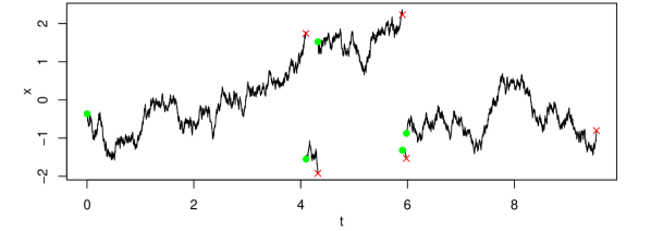
Figure 1: Path of output states of 5 tours of a Brownian Motion Restore process with $\pi\equiv\mathcal{N}(0,1^{2}),\mu\equiv\mathcal{N}(0,2^{2})$ and $C$ chosen so that $\min_{x\in\mathbbm{R}}\kappa(x)=0$. Parameters used were $\mathcal{K}=200$ and $\Lambda_{0}=1000$. The first and last output states of each tour are shown by green dots and red crosses respectively.

Indeed, when $\mu$ is a bad approximation of $\pi$, the regeneration rate can become very large. Consider $\pi$ as the 10-dimensional posterior distribution of a Logistic Regression model of breast cancer. For this model alone, we use the standard notation of letting the data, consisting of predictor-response pairs, be denoted $\{(x_{i},y_{i})\}_{i=1}^{n}$. The random variables of interest are the regression coefficients $\beta=(\beta_{1},\beta_{2},\dots,\beta_{d})^{T}$. The likelihood of a Logistic Regression model is:

$$l(\{(x_{i},y_{i})\}_{i=1}^{n}|\beta)=\left[\prod_{i=1}^{n}\frac{1}{1+\exp\{-y_{i}\beta^{T}x_{i}\}}\right].$$

See appendix I for details on the data and prior. Let $\mu\equiv\mathcal{N}(0,I)$. We generated $n=10^{5}$ samples $x_{1},x_{2},\dots,x_{n}$ from $\pi$ using the Random Walk Metropolis algorithm. A large thinning interval was used so that the Markov chain had low autocorrelation and thus the samples were of good quality. With these samples a constant $C$ such that $\kappa(x_{i})\geq 0$ for $x_{i}\in\{x_{1},x_{2},\dots,x_{n}\}$ was computed as $C=\max_{x_{1},x_{2},\dots,x_{n}}-\tilde{\kappa}(x_{i})\pi(x_{i})/\mu(x_{i})$. This value of $C$ may not be large enough to ensure that $\kappa(x)\geq 0,\forall x\in\mathbb{R}^{d}$, but suffices to demonstrate that $\kappa$ becomes very large. We estimated the quantile functions of $\tilde{\kappa}$ and $\kappa$ by evaluating these functions at $x_{1},x_{2},\dots,x_{n}$; Figure 2 shows the approximated quantile functions. We have $\mathbb{P}[\tilde{\kappa}<19.64]\approx 0.999$, but by contrast $\mathbb{P}[\kappa<9465]\approx 0.999$. Simulating a Standard Restore process with $\mathcal{K}=9465$ would be very computationally intensive. Even if simulating the inhomogeneous rate could be done without using thinning, we have $\mathbb{E}[\kappa(X)]\approx 368$, so simulation would still be slow. On the other hand, if it were possible to use $\kappa^{+}$ as the regeneration rate, truncation level $\mathcal{K}^{+}=19.64$ would be appropriate and hence simulation could be done much more efficiently.

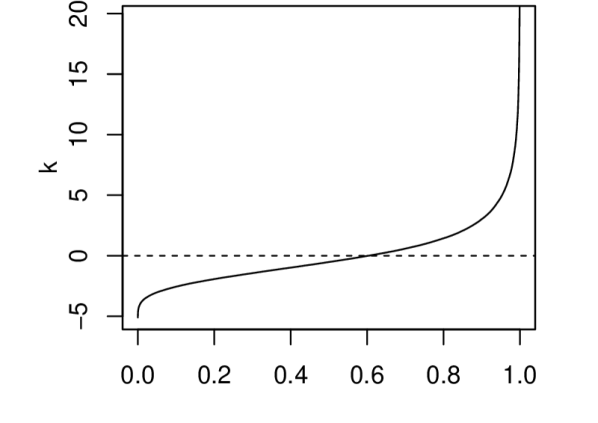
(a) $\mathbb{P}[\tilde{\kappa}(X)<k]$

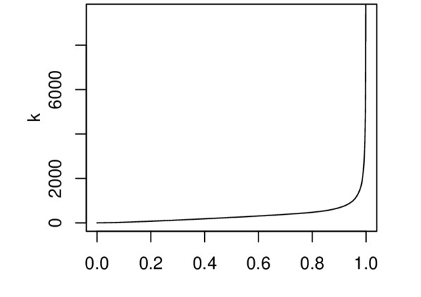
(b) $\mathbb{P}[\kappa(X)<k]$

Figure 2: Quantile functions of the partial and full regeneration rates for a Logistic Regression Model of breast cancer.

To better understand why the regeneration rate becomes so large, consider the state $x_{i^{*}}$ such that $\kappa(x_{i^{*}})=0$. This state satisfies $x_{i^{*}}=\operatorname*{arg\,max}_{x_{1},x_{2},\dots,x_{n}}-\tilde{\kappa}(x_{i})\pi(x_{i})/\mu(x_{i})$. In a sense, this is the state that is most onerous on the regeneration constant, forcing $C$ to be very large in order to compensate for the values of $\tilde{\kappa}(x_{i^{*}}),\pi(x_{i^{*}})$ and $\mu(x_{i^{*}})$. Here, one component of $x_{i^{*}}$ in the tails of $\pi$ and even further into the tails of $\mu$, meaning ratio $\mu/\pi$ is tiny. The other components are near to the mode of the corresponding marginals of $\mu$ and $\pi$, where the curvature is relatively large and hence $\tilde{\kappa}$ is negative. Thus constant $C$ must compensate for the fact that $\mu$ is poorly suited to $\pi$, which pushes up $\kappa$ in all parts of the space. Figure 3 illustrates this. The following subsection introduces the minimal regeneration distribution and rate, which may be used to ensure the regeneration rate does not become extremely large.

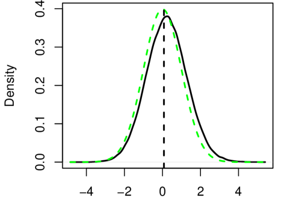
(a) $X_{5}$.

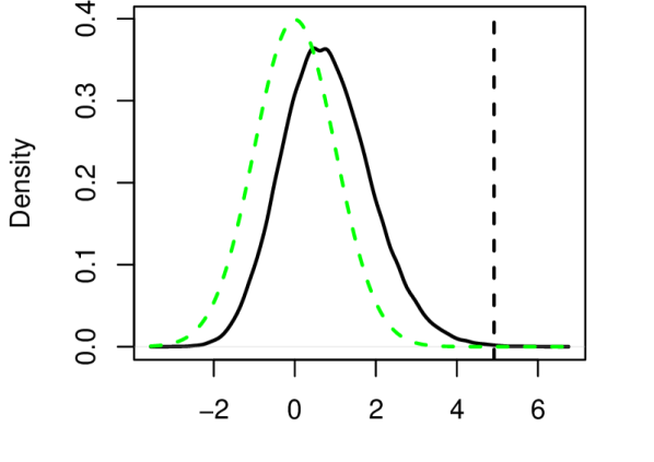
(b) $X_{9}$.

Figure 3: KDEs of marginals of $\pi$ in black. In green, $\mu$ the standard normal. Vertical dashed lines show the relevant component of $x_{i^{*}}$.

2.4.4 Minimal Brownian Motion Restore

A Minimal Brownian Motion Restore process is defined by enriching an underlying Brownian Motion with regenerations from distribution (8) at rate (7), with $\tilde{\kappa}$ given by 9. Figure 4 shows five tours of a Minimal Brownian Motion Restore process. Green dots and red crosses show the first and last output state of each tour. In this example, $\mu^{+}$ is supported on the interval $[-1,1]$, shown by gray lines. Note that the process always regenerates from outside to inside this interval and that in comparison to Figure 1, the tours of the process are on average much longer.

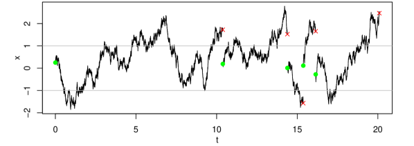
Figure 4: Five tours of a Minimal Brownian Motion Restore process with $\pi\equiv\mathcal{N}(0,1)$. The first and last output state of each tour is shown by a green dot and red cross respectively. The gray horizontal lines mark the support of $\mu^{+}$.

An advantage of Minimal Brownian Motion Restore is that it reduces computational expense. A useful feature of $\kappa^{+}$ is that to ensure $P[\kappa^{+}<\mathcal{K}^{+}]<1-\epsilon$ is satisfied, for $\epsilon>0$ a small constant (e.g. $\epsilon=0.001$), $\mathcal{K}^{+}$ scales logarithmically with dimension $d$. To see this, consider $X\sim\mathcal{N}(0,I)$. Then,

$$P[\kappa^{+}(X)<\mathcal{K}^{+}]=P[0.5(x^{T}x-d)<\mathcal{K}^{+}]=P\left[\sum_{i=1}^{d}x_{i}^{2}<2\mathcal{K}^{+}+d\right]=P[Q<2\mathcal{K}^{+}+d],$$

for $Q\sim\chi_{d}^{2}$. Figure 5 shows $\mathcal{K}^{+}$ so that $P[\kappa^{+}(X)<\mathcal{K}^{+}]<1-\epsilon$ for $\epsilon=0.01,0.001,0.0001$. Thus for a 100-dimensional Gaussian target distribution, the truncation level $\mathcal{K}^{+}=30$ would likely be appropriate. As a caveat, some functions, such as $f(x)=x^{T}x$, are very sensitive to $\mathcal{K}^{+}$ so an even more conservative choice of $\mathcal{K}^{+}$ might be necessary. Furthermore, $\tilde{\kappa}$ may prove impossible to derive in realistic situations.

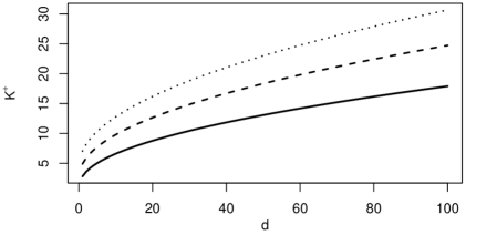
Figure 5: For $\pi\equiv\mathcal{N}(0,I)$, plot of $\mathcal{K}^{+}$ so that $P[\kappa^{+}(X)<\mathcal{K}^{+}]=1-\epsilon;\epsilon=0.01,0.001,0.0001$.

3 Adapting the Regeneration Distribution

Section 2 demonstrated that choosing the regeneration measure is challenging. Firstly, this measure must ensure that $\kappa(x)>0,\forall x\in\mathbb{R}^{d}$. Secondly, it’s desirable that the resulting $\kappa$ is not too large. An Adaptive Restore process satisfies both these properties. It is defined by enriching some underlying continuous-time Markov process with regenerations at rate $\kappa^{+}$ from, at time $t$, a distribution $\mu_{t}$. Initially, the regeneration distribution is $\mu_{0}$. The regeneration distribution is updated by adding point masses at certain time points. Let $\pi_{t}$ be the stationary distribution of the Restore process with fixed regeneration distribution $\mu_{t}$. We have simultaneous convergence of $(\mu_{t},\pi_{t})$ to $(\mu^{+},\pi)$. The density of $\mu_{t}$ is given by

$$\mu_{t}(x)=\begin{cases}\mu_{0}(x),&\text{ if }N(t)=0,\\ \frac{t}{a+t}\frac{1}{N(t)}\sum_{i=1}^{N(t)}\delta_{X_{\zeta_{i}}}(x)+\frac{a}{a+t}\mu_{0}(x),&\text{ if }N(t)>0,\end{cases}$$ (10)

where $a>0$ is some constant, $\mu_{0}$ is some fixed initial distribution and $\zeta_{1},\zeta_{2},\dots,\zeta_{N(t)}$ are the arrival times of an inhomogeneous Poisson process $(N(t)\mathrel{\mathop{\mathchar 58\relax}}t\geq 0)$ with rate

$$\begin{split}t&\mapsto\kappa^{-}(X_{t}),\\ \kappa^{-}(x)&\mathrel{\mathop{\mathchar 58\relax}}=[0\vee-\tilde{\kappa}(x)].\end{split}$$

The rate $\kappa^{-}$ Poisson process is simulated using Poisson thinning, so it is assumed that there exists a constant

$$K^{-}\mathrel{\mathop{\mathchar 58\relax}}=\sup_{x\in\mathcal{X}}\kappa^{-}(x),$$

such that $K^{-}>0$. The distribution $\mu_{t}$ is therefore a mixture of a fixed distribution $\mu_{0}$ and a discrete measure $N(t)^{-1}\sum_{i=1}^{N(t)}\delta_{X_{\zeta_{i}}}(x)$. The constant $a$ is called the discrete measure dominance time, since it is the time at which regeneration is more likely to be from the discrete measure in the mixture distribution.

Algorithm 2 describes the method. Three Poisson processes, one homogenous and two inhomogeneous, are simulated in parallel. Here, the process is generated for a fixed number of tours, though another condition such as the number of samples or simulation time could equally be used.

$t\leftarrow 0,E\leftarrow\emptyset,i\leftarrow 0,X\sim\mu_{0}.$

while $i<n$ do

       $\tilde{\tau}\sim\text{Exp}(K^{+}),s\sim\text{Exp}(\Lambda_{0}),\tilde{\zeta}\sim\text{Exp}(K^{-})$.

       if $\tilde{\tau}<s$ and $\tilde{\tau}<\tilde{\zeta}$ then

             $X\sim\mathcal{N}(X,\tilde{\tau}),t\leftarrow t+\tilde{\tau},u\sim\mathcal{U}[0,1]$.

             if $u<\kappa^{+}(X)/K^{+}$ then

                   if $|E|=0$ then

                         $X\sim\mu_{0}$.

                  else

                         $X\sim\mathcal{U}(E)$ with probability $t/(a+t)$, else $X\sim\mu_{0}$.

                   end if

                  $i\leftarrow i+1$.

             end if

            

       else if $s<\tilde{\tau}$ and $s<\tilde{\zeta}$ then

             $X\sim\mathcal{N}(X,s),t\leftarrow t+s$, record $X,t,i$.

       else

             $X\sim\mathcal{N}(X,\tilde{\zeta}),t\leftarrow t+\tilde{\zeta},u\sim\mathcal{U}[0,1]$.

             If $u<\kappa^{-}(X)/K^{-}$ then $E\leftarrow E\cup\{X\}$.

       end if

      

end while

Algorithm 2 Adaptive Brownian Motion Restore

Figure 6 shows the path of an Adaptive Restore process with $\pi\equiv\mathcal{N}(0,1),\mu_{0}\equiv\mathcal{N}(2,1)$ and $a=10$. The regeneration rate $\kappa^{+}$ encourages the process to drift to towards the origin, where the target distribution is centred. To allow convergence of the process, one might want to only record output after some burn-in time $b$.

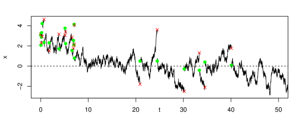
Figure 6: Path of an Adaptive Restore process with $\pi\equiv\mathcal{N}(0,1),\mu_{0}\equiv\mathcal{N}(2,1),a=10$. Green dots and red crosses show the first and last output states of each tour.

Note that for Adaptive Restore, one can’t straightforwardly apply the method described in 2.2 in order to estimate the normalizing constant $Z$. This is because we do not explicitly set constant $\tilde{C}$ and hence cannot use equation (6).

3.1 Choice of initial regeneration distribution and parameters

Generally, we set $\mu_{0}$ to approximate $\pi$, e.g., $\mu_{0}\equiv\mathcal{N}(0,I)$ ($\pi$ undergoes a pre-transformation based on its Laplace approximation, as described in Appendix B, so that the transformed $\pi$ is approximately $\mathcal{N}(0,I)$). Setting $\mu_{0}$ as a more sophisticated approximation of $\mu^{+}$ might lead to faster converge, but for the example problems considered, this simpler choice of $\mu_{0}$ suffices.

There is a tradeoff in choosing $a$, the discrete measure dominance time. Empirical experiments have shown that smaller choices of $a$ can lead to faster convergence. However, a larger value of $a$ encourages more regenerations from $\mu_{0}$, which makes it more likely for $\{X_{t}\}_{t\geq 0}$ to explore regions it has not previously visited. For the examples in this paper, we selected values of $a$ between 1,000 and 10,000.

Lastly, for the examples of this paper, $\mathcal{K}^{+}$ and $K^{-}$ were selected based on the quantile functions of $\tilde{\kappa}$, approximated using the output of a preliminary Markov chain run generated with a Metropolis-Hastings algorithm. It may be possible to learn suitable values of $\mathcal{K}^{+}$ and $K^{-}$ on-the-fly, without the need for a preliminary run of a Markov chain. Assuming $\pi$ is $d$-dimensional and close to Gaussian, a sensible initial guess of $K^{-}$ is $d/2$ (see 2.4.4), which could then be adjusted as necessary. Similarly, a sensible initial estimate for $\mathcal{K}^{+}$ could be made based on the cumulative distribution function of a chi-squared random variable (again see 2.4.4) then adjusted by monitoring how often $\kappa$ exceeds this truncation level.

3.2 Connections with ReScaLE

Although inspired by the Restore algorithm of Wang et al., (2021), the Adaptive Restore algorithm presented in Algorithm 2 has many connections to quasi-stationary Monte Carlo (QSMC) methods such as the ScaLE Algorithm of Pollock et al., 2020b , and particularly the ReScaLE algorithm of Kumar, (2019).

Indeed, ScaLE and ReScaLE can be seen as instances of Restore where the regeneration distribution is chosen to be the target, which is then learnt adaptively: the killing rate for QSMC methods is given by

$$\kappa=\tilde{\kappa}+C,$$

and in the case of ReScaLE, at a killing time $T$, the process is regenerated from its empirical occupation measure:

$$X_{T}\sim\frac{1}{T}\int_{0}^{T}\delta_{X_{s}}\operatorname{d\!}s.$$ (11)

The key motivation behind ScaLE and ReScaLE was applicability to tall data problems, due to the applicability of exact subsampling techniques Pollock et al., 2020b ; Kumar, (2019), however sampling from (11) is somewhat delicate due to the need to simulate complex diffusion bridges.

By contrast, although Adaptive Restore does not straightforwardly permit exact subsampling, its regeneration mechanism is considerably simpler to implement, and it is only required to adaptively learn the compactly-supported distribution $\mu^{+}$. ReScaLE need learn the entire distribution $\pi$—approximated by the trajectory of the diffusion path – on $\mathbb{R}^{d}$ for its regeneration mechanism, and thus the two algorithms—although similar in many regards—can be seen as complementary.

4 Theory

In this section we will establish the validity of the Adaptive Restore algorithm, as described in Algorithm 2. In general, this is a difficult task since the process is self-reinforcing, on a noncompact state space; most works in the literature are for compact state spaces, an exception being Mailler and Villemonais, (2020). In our present setting, we will thus establish validity by showing that the measures $\mu_{t}$ in (10) converges weakly almost surely to the minimal regeneration distribution $\mu^{+}$ as in (8), which ultimately implies validity of the Adaptive Restore algorithm. For this theoretical analysis, we consider a fixed regeneration rate; in particular we do not consider questions related to truncating a possibly divergent regeneration rate.

This section is self-contained, to be illustrated by numerical experiments in Section 5.

4.1 Summary of theoretical contributions and related work

The theoretical analysis in this section is based on stochastic approximation techniques, following a similar overall approach as in the sequence of previous works already cite. Our proof most closely follows the approaches of Benaïm et al., (2018); Wang et al., (2020), with several key novelties. The former shows almost sure convergence of stochastic approximation algorithms for discrete-time processes on compact spaces. By focussing our attention on the measures $\mu_{t}$, which in our present setting are supported on a compact set, we will be able to identify an appropriate embedded discrete-time Markov chain, to which we can apply their main results. Thus the main technical work of this section is identifying the appropriate discrete-time structure, and then checking that the relevant hypotheses are satisfied.

A further difference between our present analysis and the previous works cited above concerns the nature of the killing mechanism. In all previous works, the killing mechanism was given by an additional random clock $\tau_{\partial}$ of the form

$$\tau_{\partial}\mathrel{\mathop{\mathchar 58\relax}}=\inf\left\{s\geq 0\mathrel{\mathop{\mathchar 58\relax}}\int_{0}^{s}\kappa(X_{u})\operatorname{d\!}u\geq\xi\right\},$$ (12)

for an appropriate killing rate $\kappa\mathrel{\mathop{\mathchar 58\relax}}\mathcal{X}\to[0,\infty]$ and $\xi\sim\mathrm{Exp}(1)$ independent (in discrete-time settings the obvious modifications need to be made).

By contrast, our present setting is considering two competing clocks $\zeta$ and $T$, each of which defined as in (12) with their own respective arrival rates $\kappa^{\pm}$ and independent exponential random variables $\xi,\xi^{\prime}$. A ‘killing’ event in our setting is then the event

$$\zeta<T,$$

namely that the clock with rate $\kappa^{-}$ rings before the clock with rate $\kappa^{+}$.

Even with these key differences, we show in this section that the general stochastic approximation approach of Benaïm et al., (2018); Wang et al., (2020) can still be applied, and thus we deduce almost sure weak convergence of the measures $\mu_{t}$.

4.2 Diffusion setting and Restore process

We assume that we are given some underlying local dynamics on the Euclidean space $\mathbb{R}^{d}$, with generator $L$, assumed to be a self-adjoint (reversible) diffusion:

$$\operatorname{d\!}X_{t}=\nabla A(X_{t})\operatorname{d\!}t+\operatorname{d\!}W_{t}.$$ (13)

For simplicity one can assume (13) to be a Brownian motion with $A\equiv 0$. This is a symmetric diffusion, with a self-adjoint generator $L$ on the Hilbert space $\mathcal{L}^{2}(\Gamma)$, where

$$\Gamma(\operatorname{d\!}y)=\gamma(y)\operatorname{d\!}y,\quad\gamma(y)=\exp(2A(y)),\quad\forall y\in\mathbb{R}^{d}.$$

For Brownian motion, $\Gamma$ reduces to Lebesgue measure, and we often work in that case for notational simplicity; but the analysis extends to the more general reversible case.

We have fixed a target density $\pi$ on $\mathbb{R}^{d}$. We then define a partial killing rate $\tilde{\kappa}$, which comes from Wang et al., (2019): $\tilde{\kappa}\mathrel{\mathop{\mathchar 58\relax}}\mathbb{R}^{d}\to\mathbb{R}$,

$$\tilde{\kappa}(y)\mathrel{\mathop{\mathchar 58\relax}}=\frac{1}{2}\left(\frac{\Delta\pi}{\pi}-\frac{2\nabla A\cdot\nabla\pi}{\pi}-2\Delta A\right)(y),\quad y\in\mathbb{R}^{d}.$$

In the special case of Brownian motion ($A\equiv 0$), this reduces to (9).

We then define the positive and negative parts:

$$\kappa^{+}\mathrel{\mathop{\mathchar 58\relax}}=\tilde{\kappa}\vee 0,\qquad\kappa^{-}\mathrel{\mathop{\mathchar 58\relax}}=-(\tilde{\kappa}\wedge 0).$$

We make the following regularity assumptions (c.f. Wang et al., (2019)).

Assumption 1.

$A$ is smooth ($C^{\infty}$), such that the SDE (13) has a unique nonexplosive weak solution. The target density $\pi$ is smooth and positive, and that $\int\pi^{2}/\exp(2A)\operatorname{d\!}y<\infty$. Thus $\tilde{\kappa}$ is continuous, which implies that the functions $\kappa^{+},\kappa^{-}$ are continuous.

Furthermore, $\kappa^{-}\leq K^{-}$ uniformly for some $K^{-}>0$.

Assumption 2.

The support of $\kappa^{-}$ is bounded: the set

$$\mathcal{X}\mathrel{\mathop{\mathchar 58\relax}}=\{x\in\mathbb{R}^{d}\mathrel{\mathop{\mathchar 58\relax}}\tilde{\kappa}(x)\leq 0\}$$

is a compact subset of $\mathbb{R}^{d}$.

Remark 1.

When we use Brownian motion as local dynamics, this is a weak condition, holding for instance when $\pi$ satisfies a suitable sub-exponential tail condition (Wang et al.,, 2019).

Thus, the sub-Markov semigroup corresponding to the diffusion $X$, killed at rate $\kappa^{+}$ can also be realised as a self-adjoint semigroup on $\mathcal{L}^{2}(\Gamma)$. Furthermore, there exists a transition sub-density $p^{\kappa^{+}}(t,x,y)$, as in Kolb and Steinsaltz, (2012), following from the derivation of Demuth and van Casteren, (2000): writing $T_{1}$ for the first killing event,

$$\mathbb{E}_{x}[f(X_{t})\mathbb{I}_{t<T_{1}}]=\int p^{\kappa^{+}}(t,x,y)f(y)\,\operatorname{d\!}y.$$ (14)

From Demuth and van Casteren, (2000), the function $(t,x,y)\mapsto p^{\kappa^{+}}(t,x,y)$ will be jointly continuous and symmetric in $x,y$.

Assumption 3.

The killing time $T_{1}$ has uniformly bounded expectation on $\mathcal{X}$: $\sup_{x\in\mathcal{X}}\mathbb{E}_{x}[T_{1}]<\infty.$

Remark 2.

This is a very weak assumption, since $\mathcal{X}$ is a compact set. A much stronger condition will be satisfied—uniform bounded expectation over the entirety of $\mathbb{R}^{d}$ for Brownian motion—if the killing rate satisfies

$$\liminf_{\|x\|\to\infty}\tilde{\kappa}(x)>0,$$

which is the case when $\pi$ possesses a sub-exponential tail; see Wang et al., (2019).

We shall also require the following elementary identity.

Lemma 4.1.

For any $x\in\mathcal{X}$, we have the identity

$$\mathbb{E}_{x}[T_{1}]=\int_{0}^{\infty}\operatorname{d\!}t\int\operatorname{d\!}y\,p^{\kappa^{+}}(t,x,y).$$

4.3 Restore process

Recall the minimal regeneration distribution, as in (8), which has a density function with respect to Lebesgue measure on $\mathbb{R}^{d}$, compactly supported on $\mathcal{X}$, given by

$$\mu^{+}(y)\mathrel{\mathop{\mathchar 58\relax}}=\frac{1}{C^{+}}\pi(y)\kappa^{-}(y),$$

where $C^{+}\mathrel{\mathop{\mathchar 58\relax}}=\int\pi(y)\kappa^{-}(y)\operatorname{d\!}y$ is the normalizing constant.

We consider now running a Restore process $X$ with local dynamics (13) described by infinitesimal generator $L$, regeneration rate $\kappa^{+}$ and regeneration distribution $\mu$. If $\mu=\mu^{+}$, then $\pi$ will be the invariant distribution of $X$ under appropriate regularity conditions; see Wang et al., (2021).

The goal of the Adaptive Restore algorithm is to learn $\mu^{+}$ adaptively, by running an additional Poisson process with rate function

$$t\mapsto\kappa^{-}(X_{t}).$$

These auxiliary arrival times will be used to construct the adaptive estimate of $\mu^{+}$.

Notationally, we will use letters $T,T_{1},T_{2},\dots$ to refer to regeneration times of the Restore process, which arrive with rate $\kappa^{+}(X_{t})$, and $\zeta,\zeta_{1},\zeta_{2},\dots$ to refer to the addition events which arrive with rate $\kappa^{-}(X_{t})$.

In particular, for a Restore process with local dynamics $L$, regeneration rate $\kappa^{+}$ and regeneration distribution $\mu$—abbreviated into Restore($L,\kappa^{+},\mu)$—we have, $X_{T_{i}}\sim\mu$.

We have the following representation from Wang et al., (2021) of the invariant measure of Restore$(L,\kappa,\mu)$:

$$\Pi_{\kappa}(\mu)(\operatorname{d\!}y)\propto\int\mu(\operatorname{d\!}x)\int_{0}^{\infty}\operatorname{d\!}t\,p^{\kappa}(t,x,y)\operatorname{d\!}y.$$

In particular, we must therefore have the identity

$$\pi(y)\propto\int\mu^{+}(\operatorname{d\!}x)\int_{0}^{\infty}\operatorname{d\!}t\,p^{\kappa^{+}}(t,x,y).$$ (15)

4.4 Discrete-time system

For now we imagine the rebirth distribution to be a fixed (but arbitrary) measure $\mu$ and consider the Restore($L,\kappa^{+},\mu)$ process, with additional events $(\zeta_{i})_{i=1}^{\infty}$ at rate $\kappa^{-}(X_{t})$. We will let $\mathbb{E}_{x}$ denote the expectation under the law of this Restore process $X$ initialised from $X_{0}=x$. We are interested in studying the behaviour of the points $(X_{\zeta_{1}},X_{\zeta_{2}},\dots)$.

Our first goal is to show that this sequence is in fact a Markov chain, and give an expression for its transition kernel. To reduce notational clutter, we will write $\zeta\mathrel{\mathop{\mathchar 58\relax}}=\zeta_{1}$, and $T\mathrel{\mathop{\mathchar 58\relax}}=T_{1}$ for the first $\kappa^{-}$ or regeneration events respectively:

$$\begin{split}\zeta&\mathrel{\mathop{\mathchar 58\relax}}=\inf\left\{s\geq 0\mathrel{\mathop{\mathchar 58\relax}}\int_{0}^{s}\kappa^{-}(X_{u})\operatorname{d\!}u\geq\xi\right\},\\ T&\mathrel{\mathop{\mathchar 58\relax}}=\inf\left\{s\geq 0\mathrel{\mathop{\mathchar 58\relax}}\int_{0}^{s}\kappa^{+}(X_{u})\operatorname{d\!}u\geq\xi^{\prime}\right\},\end{split}$$

where $\xi,\xi^{\prime}\sim\mathrm{Exp}(1)$ are independent of each other and of all other random variables.

Lemma 4.2.

Defining for each $i\in\mathbb{N}$, $Y_{i}\mathrel{\mathop{\mathchar 58\relax}}=X_{\zeta_{i}}$, the sequence $(Y_{i})_{i=1}^{\infty}$ is a Markov chain on $\mathcal{X}$.

Proof.

This follows from the fact that the underlying Restore process $X$ is a strong Markov process, and the fact that the Poisson processes have independent exponential random variables. ∎

We now define a Markov sub-kernel $Q(x,\operatorname{d\!}y)$ on $\mathcal{X}$ which will be crucial to describing the transition kernel of the chain $Y$. The kernel is defined, for any integrable $f\mathrel{\mathop{\mathchar 58\relax}}\mathcal{X}\to\mathbb{R}$, by

$$Qf(x)\mathrel{\mathop{\mathchar 58\relax}}=\mathbb{E}_{x}[f(X_{\zeta})\,\mathbb{I}_{\zeta<T}].$$

We can then define $q\mathrel{\mathop{\mathchar 58\relax}}\mathcal{X}\to[0,1]$ by

$$q(x)\mathrel{\mathop{\mathchar 58\relax}}=1-Q1(x)=1-\mathbb{P}_{x}(\zeta<T)=\mathbb{P}_{x}(T\leq\zeta).$$

We can also define a proper Markov kernel,

$$Q_{0}(x,\cdot)\mathrel{\mathop{\mathchar 58\relax}}=\frac{Q(x,\cdot)}{Q(x,\mathcal{X})}=\mathbb{E}_{x}[f(X_{\zeta})|\zeta<T].$$

We need the following technical result; namely, we check (Benaïm et al.,, 2018, Hypotheses H1, H2).

Lemma 4.3.

$Q$ is Feller, and defining the augmented kernel $\bar{Q}$ on $\mathcal{X}\cup\{\partial\}$, where $\partial\notin\mathcal{X}$ represents an absorbing state,

$$\bar{Q}(x,\operatorname{d\!}y)\mathrel{\mathop{\mathchar 58\relax}}=Q(x,\operatorname{d\!}y)\mathbb{I}_{x\in\mathcal{X}}+q(x)\delta_{\partial}(\operatorname{d\!}y)\mathbb{I}_{x\in\mathcal{X}}+\delta_{\partial}(\operatorname{d\!}y)\mathbb{I}_{x\in\{\partial\}},$$

we have that $\partial$ is accessible for $\bar{Q}$.

Proof.

The Feller property holds by the representation (14). Accessibility of $\partial$ is immediate, since started from anywhere, the diffusion path can (eventually) be killed. ∎

Proposition 4.4.

The Markov chain $Y$ has transition kernel $Q_{\mu}(x,\operatorname{d\!}y)$ on $\mathcal{X}$ given by

$$\begin{split}Q_{\mu}(x,\operatorname{d\!}y)&=Q(x,\operatorname{d\!}y)+q(x)\frac{\mu Q(\operatorname{d\!}y)}{\mu Q1}\\ &=\left(1-q(x)\right)Q_{0}(x,\operatorname{d\!}y)+q(x)\frac{\mu Q(\operatorname{d\!}y)}{\mathbb{P}_{\mu}(\zeta<T)}.\end{split}$$

4.5 Adaptive reinforced process

We are interested in studying the limiting behaviour of

$$\mu_{n}\mathrel{\mathop{\mathchar 58\relax}}=\frac{1}{n}\sum_{i=1}^{n}\delta_{Y_{i}},$$

where now the $(Y_{i})$ are generated as follows:

$$Y_{n+1}|(Y_{0},Y_{1},\dots,Y_{n})\sim Q_{\mu_{n}}(Y_{n},\cdot).$$ (16)

This corresponds to our Adaptive Restore algorithm (Algorithm 2), where we are learning an approximation to the minimal rebirth distribution. Our goal will be to show the almost sure weak convergence of $\mu_{n}\to\mu^{+}$ as $n\to\infty$. We will utilise the approach of Benaïm et al., (2018).

4.6 Fixed point analysis

In order to understand the limiting properties of the self-reinforcing process $(Y_{i})$ in (16), we need to study the properties of the $Q_{\mu}$ kernels.

We have the following useful representation. We write $\mathcal{P}(\mathcal{X})$ for the space of probability measures on $\mathcal{X}$.

Lemma 4.5.

For any bounded continuous $f$, we have for $x\in\mathcal{X}$,

$$\mathcal{A}f(x)\mathrel{\mathop{\mathchar 58\relax}}=\sum_{n\geq 1}Q^{n}(x,f)=\int_{0}^{\infty}\operatorname{d\!}t\int\operatorname{d\!}y\,p^{\kappa^{+}}(t,x,y)f(y)\kappa^{-}(y).$$

The nonnegative kernel $\mathcal{A}$ is also a bounded kernel on $\mathcal{X}$: $\mathcal{A}1(x)\leq\|\mathcal{A}\|_{\infty}<\infty$. Furthermore, there exists $\delta>0$ such that for any $x\in\mathcal{X}$, $\delta\leq\mathcal{A}1(x)$. This implies Lipschitz continuity (with respect to total variation) of the map $\mathcal{P}(\mathcal{X})\to\mathcal{P}(\mathcal{X})$ given by

$$\mu\mapsto\Pi_{\mu}\mathrel{\mathop{\mathchar 58\relax}}=\frac{\mu\mathcal{A}}{\mu\mathcal{A}1}.$$

Proposition 4.6.

Given a fixed probability measure $\mu$ on $\mathcal{X}$, the invariant distribution of the kernel $Q_{\mu}$ is proportional to $\mu\mathcal{A}$, where $\mathcal{A}$ is the kernel $\sum_{n\geq 1}Q^{n}$.

4.7 Limiting ODE flow

The limiting flow can be defined just as in Benaïm et al., (2018, Section 5), since we have the appropriate assumptions in force; Lemma 4.3 and also the Lipschitz property of $\mu\mapsto\Pi_{\mu}$, Lemma 4.5. In other words, we also have, from Benaïm et al., (2018, Proposition 5.1), an injective semi-flow $\Phi$ on $\mathcal{P}(\mathcal{X})$ such that $t\mapsto\Phi_{t}(\mu)$ is the unique weak solution to

$$\dot{\mu}_{t}=-\mu_{t}+\Pi_{\mu_{t}},\quad\mu_{0}=\mu.$$

We need to check global asymptotic stability, and to do this we will follow the approach in Wang et al., (2020).

In particular, we need to identify the eigenfunctions of $\mathcal{A}$.

Proposition 4.7.

We have that, for $\mu^{+}$ the minimal rebirth distribution, $\mu^{+}\mathcal{A}\propto\mu^{+}$, and defining $\varphi\mathrel{\mathop{\mathchar 58\relax}}=\pi|_{\mathcal{X}}$ to be the restriction of $\pi$ to $\mathcal{X}$, $\mathcal{A}\varphi=\beta\varphi$, where $\beta\mathrel{\mathop{\mathchar 58\relax}}=C^{+}\mathbb{E}_{\mu^{+}}[T_{1}]$.

Given the preceding results, we can now conclude the following.

Proposition 4.8.

We have that $\mu^{+}$ is a global attractor for the semi-flow $\Phi$: we have convergence $\Phi_{t}(\mu)\to\mu^{+}$ uniformly in $\mu$ in total variation distance.

Proof.

Since we have obtained uniform upper and lower bounds on $0<\delta\leq\mathcal{A}1(x)\leq K^{-}\sup_{x\in\mathcal{X}}[T_{1}]$ from Lemma 4.5, the proof is identical to the proof of Wang et al., (2020, Theorem 3.6), and hence omitted. ∎

4.8 Asymptotic pseudo-trajectories

We secondly need to demonstrate that our trajectories $(n\mapsto\mu_{n})$, once suitably embedded in continuous time, are an asymptotic pseudo-trajectory for the semi-flow $\Phi$ defined in Section 4.7.

The key technical challenge to establishing this is to prove an analogue of Benaïm et al., (2018, Lemma 6.2) in our setting. Once that is in place, everything else follow identically from Benaïm et al., (2018, Section 6).

We need the following Lipschitz property, where the total variation norm for a signed measure $\nu$ on $\mathcal{X}$ is defined as

$$\|\nu\|_{\mathrm{TV}}\mathrel{\mathop{\mathchar 58\relax}}=\sup\{|\nu(f)|\mathrel{\mathop{\mathchar 58\relax}}f\mathrel{\mathop{\mathchar 58\relax}}\mathcal{X}\to\mathbb{R}\text{ bounded measurable, }\|f\|_{\infty}\leq 1\}.$$

Lemma 4.9.

For probability measures $\mu,\nu\in\mathcal{P}(\mathcal{X})$ and $j\in\mathbb{N}$, with $C_{\mathrm{L}}\mathrel{\mathop{\mathchar 58\relax}}=2/\delta$,

$$\sup_{\alpha\in\mathcal{P}(\mathcal{X})}\|\alpha Q_{\mu}^{j}-\alpha Q_{\nu}^{j}\|_{\mathrm{TV}}\leq C_{\mathrm{L}}2^{j}\|\mu-\nu\|_{\mathrm{TV}},$$

and for each bounded function $f$,

$$\sup_{x\in\mathcal{X}}\|Q_{\mu}^{j}(x,f)-Q_{\nu}^{j}(x,f)\|_{\mathrm{TV}}\leq C_{\mathrm{L}}2^{j}\|f\|_{\infty}\|\mu-\nu\|_{\mathrm{TV}}.$$

With this result, the rest of the approach of Benaïm et al., (2018, Section 6) goes through to establish the desired result.

Theorem 4.10.

Under our Assumptions 1–3, almost surely, the sequence $(\mu_{n})$ converges weakly to the minimal regeneration distribution $\mu^{+}$.

Proof.

By embedding the sequence $(\mu_{n})$ into continuous time as in Benaïm et al., (2018, Section 6.1), the resulting process $(\hat{\mu}_{t})$ is an asymptotic pseudo-trajectory of $\Phi$, by Lemma 4.9 and Benaïm et al., (2018, Theorem 6.4). Combined with Proposition 4.8, this proves the result; see Benaïm, (1999). ∎

5 Examples

The examples presented show that Adaptive Restore can significantly decrease the truncation level used for simulation of the algorithm. This is especially the case when $\pi$ has skewed tails.

5.1 Transformed Beta Distribution

We experiment with sampling from a distribution with density

$$\pi(x)=6e^{2x}(e^{x}+1)^{-4}.$$

Appendix J explains how this distribution is derived from the transformation of a Beta distribution. It happens that $\tilde{\kappa}(x)<2,\forall x\in\mathbb{R}$, which makes this distribution a useful test case, since an Adaptive Restore process may be efficiently simulated without any truncation of the regeneration rate. In addition, the first and second moments, 0 and $(\pi^{2}-6)/3$, may be computed analytically. Here, $K^{-}=0.5$. Taking $\mu_{0}\equiv\mathcal{N}(0.5,1)$ we simulated 200 Adaptive Restore processes each with a burn-in period of $b=5\,10^{6}$ followed by a period of length $10^{6}$ during which output was recorded at rate 10. We deliberately chose $\mu_{0}$ to be centred away from the mean of $\pi$, in order to test that the process still converges. The discrete measure dominance time was $1000$: $106$ estimates of first moment were greater than the exact first moment; $98$ estimates of the second moment were greater than the exact second moment. This indicates the processes have (approximately) converged to the correct invariant distribution.

5.2 Logistic Regression Model of Breast Cancer

We used Adaptive Restore to simulate from the (transformed) posterior of a Logistic Regression model of breast cancer ($d=10$). This model was first used in 2.4.3 to demonstrate that $\mathcal{K}$ can become very large; in this case, for Standard Restore with $\mu\equiv\mathcal{N}(0,I)$, a sensible choice is $\mathcal{K}=9465$. Details of the data and prior are given in appendix I.

We simulated an Adaptive Restore process with $\mu_{0}\equiv\mathcal{N}(0,I_{d})$ and parameters $K^{-}=5.2,\mathcal{K}^{+}=19.64,\Lambda_{0}=10.0,a=1000$, $b=6\,10^{6}$, $T=10^{6}$. We chose a long burn-in time because other experiments have shown that this is necessary for convergence of $(\mu_{t},\pi_{t})$. To check the estimate, we generated $10^{6}$ samples using the Random Walk Metropolis algorithm, first tuning the scale of the symmetric proposal distribution and using a thinning interval of 50 so that the samples had small autocorrelation. Figure 7 plots the estimate of the mean of each marginal for the Random Walk Metropolis estimate (circles) and the Adaptive Restore estimate (crosses). The Euclidean distance between these estimates was 0.014 (2.s.f).

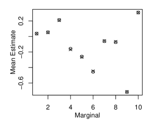
Figure 7: Estimates of the mean of each marginal of the (transformed) posterior distribution of a Logistic Regression model of Breast Cancer. Circles show a Random Walk Metropolis estimate, crosses an Adaptive Restore estimate.

5.3 Hierarchical Model of Pump Failure

Consider the following hierarchical model of pump failure (Carlin and Gelfand,, 1991):

$$R_{i} \sim\text{Poisson}(X^{\prime}_{i}t_{i});i=1,2,\dots,10;$$

$$X^{\prime}_{i} \sim\text{Gamma}(c_{1},X^{\prime}_{11});i=1,2\dots,10;$$

$$X^{\prime}_{11} \sim\text{InverseGamma}(c_{2},c_{3});$$

with constants $c_{1}=1.802,c_{2}=2.01,c_{3}=1.01$. Observation $R_{i}\leavevmode\nobreak\ (i=1,2,\dots,10)$ is the number of recorded failures of pump $i$, which is observed for a unit of time $t_{i}\leavevmode\nobreak\ (i=1,2,\dots,10)$. The failure rate of pump $i$ is $X^{\prime}_{i}\leavevmode\nobreak\ (i=1,\dots,10)$. Before sampling, we transformed the posterior to be defined on $\mathbb{R}^{d}$ by making a change-of-variables, defining $X_{i}=\log X^{\prime}_{i}\leavevmode\nobreak\ (i=1,\dots,10)$. We then transformed the posterior again, based on its Laplace approximation, as described in Appendix B.

The posterior exhibits heavy and skewed tails. Because of this, under Standard Restore with an isotropic Gaussian regeneration distribution, we have $\mathbbm{E}_{\pi}[\kappa(X)]\approx 1.9\times 10^{7}$, far too large for simulation to be practical. By contrast, $\mathbbm{E}_{\pi}[\kappa^{+}(X)]\approx 1$. We are able to accurately compute the first moment of the posterior in less than an hour of simulation time.

5.4 Log-Gaussian Cox Point Process Model

A Log-Gaussian Cox Point Process models a $[0,1]^{2}$ area divided into a $n\times n$ grid. The number of points $Y=\{Y_{i,j}\}$ in each cell is conditionally independent given latent intensity $\Lambda=\{\Lambda_{i,j}\}$ and has Poisson distribution $n^{2}\Lambda_{i,j}=n^{2}\exp\{X_{i,j}\}$. The latent field is $X=\{X_{i,j}\}$. Assume $X$ is a Gaussian process with mean vector zero and covariance function

$$\Sigma_{(i,j),(i^{\prime},j^{\prime})}=\exp\{-\delta(i,i^{\prime};j,j^{\prime})/n\},$$

where $\delta(i,i^{\prime};j,j^{\prime})=((i-i^{\prime})^{2}+(j-j^{\prime})^{2})^{1/2}$. We have:

$$\log\pi(x|y)=\sum_{i,j}y_{i,j}x_{i,j}-n^{2}\exp\{x_{i,j}\}-\frac{1}{2}x^{T}\Sigma^{-1}x+\text{const}.$$

We present results for simulated data on a 5 by 5 grid, so $d=25$. After transformation (again, see Appendix B), the posterior distribution of this model is close to an Isotropic Gaussian distribution. For standard Restore setting $\mu\equiv\mathcal{N}(0,I)$ results in $\mathbb{P}[\kappa(X)<181]\approx 0.9999$ and $\mathbb{E}[\kappa(X)]\approx 19.5$. Thus $\mathcal{K}=181$ would be appropriate.

For Adaptive Restore we have $\mathbb{P}[\kappa^{+}<18.5]\approx 0.9999$ and $\mathbb{E}[\kappa^{+}(X)]\approx 1.4$. Thus Adaptive Restore reduces both the necessary truncation level and average regeneration rate by a factor of 10. However, simulation runs indicate that convergence of the Adaptive process for this $d=25$ posterior is slow. Though $\mu_{t}$ does not need to adapt to account for skew so much, it still needs to change significantly so that it is centred correctly—this is harder in higher dimensions.

5.5 Multivariate t-distribution

Recall that a $d$-dimensional multivariate t-distribution with mean $m$, scale matrix $\Sigma$ and $\nu$ degrees of freedom has density:

$$\pi(x)\propto\left[1+\frac{1}{\nu}(x-m)^{T}\Sigma^{-1}(x-m)\right]^{-(\nu+d)/2}.$$

We consider sampling from a bivariate t-distribution with $\nu=10$, zero mean and identity scale matrix. We then have $\kappa^{+}(x)<1.55,\forall x\in\mathbb{R}^{d}$ (this bound is not tight), so can take $K^{+}=1.55$ (no need to truncate $\kappa$). In general, Restore processes are particularly well suited to simulating from t-distributions, since the regeneration rate is naturally bounded. For this example, we can take $K^{-}=1.2$. The process is quickly able to recover the true variance of each marginal of the target distribution, which is $\nu/(\nu-2)$. Figure 8 shows contours of $\tilde{\kappa},\kappa^{+}$ and $\mu^{+}$. A notable feature is that, moving outwards from the origin, $\kappa^{+}$ rises to its maximum value then asymptotically tends to zero.

(a) $\tilde{\kappa}$

(b) $\kappa^{+}$ and $\mu^{+}$

Figure 8: Contours of $\tilde{\kappa},\kappa^{+}$ and $\mu^{+}$ for $\pi$ a bivariate t-distribution with $\nu=10$.

5.6 Mixture of Gaussian distributions

Multi-modal posterior distributions sometimes arise in Bayesian modelling problems. For example, the standard two-parameter Ising model (Geyer,, 1991) is bimodal for some parameter combinations; a model of a problem concerning sensor network location (Ihler et al.,, 2005) is a popular example that features in many papers (Ahn et al.,, 2013; Lan et al.,, 2014; Pompe et al.,, 2020). Standard MCMC algorithms struggle to sample multi-modal distributions because the area of low probability density between modes acts as a barrier that is difficult to cross. Several techniques have been developed specifically for multi-modal posteriors, which generally fall under tempering (Geyer,, 1991; Marinari and Parisi,, 1992) and mode-hopping strategies (Tjelmeland and Hegstad,, 2001; Ahn et al.,, 2013).

We explore the use of an Adaptive Restore process for simulating from the Gaussian mixture distribution

$$\pi(x)=w_{1}\mathcal{N}(x;m_{1},\Sigma_{1})+w_{2}\mathcal{N}(x;m_{2},\Sigma_{2}),$$

for $w_{1}=0.4,w_{2}=0.6,m_{1}=(1.05,1.05),m_{2}=(-1.05,-1.05)$,

$$\Sigma_{1}=\begin{pmatrix}1&-0.1\\ -0.1&1\end{pmatrix}\text{and }\Sigma_{2}=\begin{pmatrix}1&0.1\\ 0.1&1\end{pmatrix}.$$

Figure 9 shows contour plots of the density of $\pi$ and $\kappa^{+}$. In particular, figure 9(b) shows that the region for which $\kappa^{+}$ is zero, which corresponds to the support of $\mu^{+}$, consists of two separate non-connected areas. For Standard Restore and Adaptive Restore, we set $\mu$ and $\mu_{0}$ respectively to $\mathcal{N}(0,3I)$.

Standard Restore was able to sample from this distribution well, even though we had to set $\mathcal{K}=1000$ so that the truncation wouldn’t overly affect $\kappa$. Setting $\Lambda_{0}=10$, a simulation time of $T=10000$ generated samples which produced an estimate of the mean that had Root Mean Square Error (RMSE) 0.00358 (3.s.f). Simulation took 3.5 minutes.

By comparison, Adaptive Restore allows the truncation level to be much reduced, to $K^{+}=20$. We set $a=10,000$ to allow both modes to be explored before the discrete measure became dominant. A burn-in time of $b=900,000$ and simulation time of $T=100,000$ took 6 minutes. Setting $\Lambda_{0}=1$, so that in expectation the number of samples produced equals that for Standard Restore, the RMSE was 0.0555 (3.s.f).

In analogue to similar schemes based on stochastic approximation Aldous et al., (1988); Blanchet et al., (2016); Benaïm et al., (2018); Mailler and Villemonais, (2020), this slow convergence is a result of the urn-like behaviour intrinsic to such methods. Although the chain is guaranteed to converge asymptotically, in finite time the chain is naturally inclined to visit regions it has visited before. For example, even on a finite state space, Benaïm and Cloez, (2015, Corollary 1.3) shows convergence can occur in some cases at a very slow polynomial rate.

Thus in practice, we suggest a judicious choice of initial distribution $\mu_{0}$ and constant $a$ as in Algorithm 2, to ensure that the measures $\mu_{t}$ quickly place some mass in all modes of the target distribution.

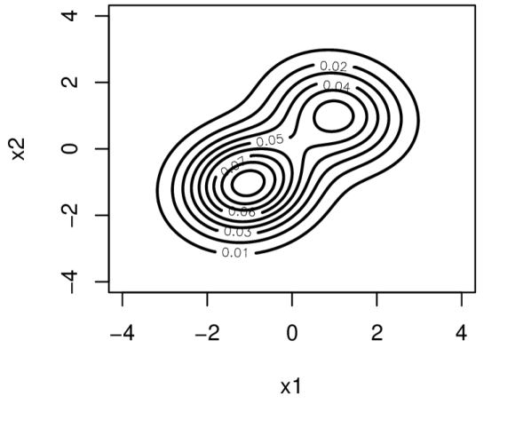
(a) $\pi$

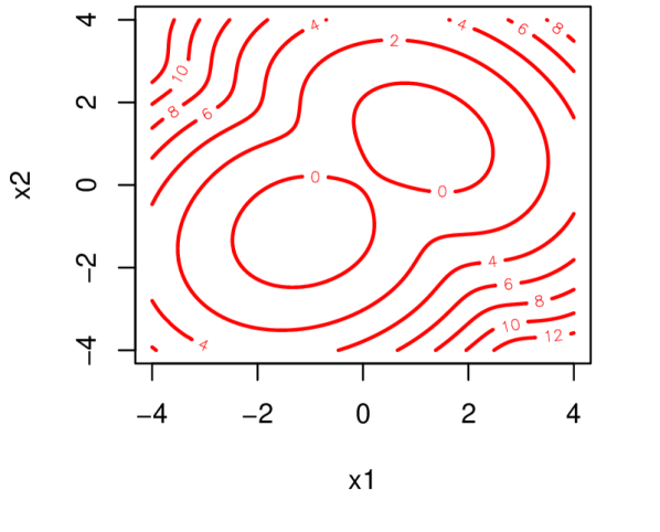
(b) $\kappa^{+}$

Figure 9: Density of $\pi$ and $\kappa^{+}$ for $\pi$ a mixture of bivariate Gaussian distributions.

6 Discussion

This article has introduced the Adaptive Restore process, an extension of the Restore process (Wang et al.,, 2021), which adapts the regeneration distribution on the fly. Like Standard Restore, Adaptive Restore benefits from global moves. For target distributions that are hard to approximate with a parametric distribution, Adaptive Restore is more suitable than Standard Restore, because its use of the minimal regeneration rate makes simulation computationally feasible. In comparison to simpler algorithms such as Random Walk Metropolis, the process can still be slow to simulate and convergence appears to be slow when the target is multimodal. However, the algorithm shows promise in sampling distributions with skewed tails, for which Standard Restore can be computationally intractable. From a theoretical perspective, we have demonstrated how the framework of stochastic approximation can be successfully applied to a novel class of Markov processes.

Global dynamics allow the Adaptive Restore process to make large moves across the space, a property shared by Standard Restore. This feature is desirable for MCMC samplers (since it results in a Markov chain with smaller autocorrelation) and has motivated the development of algorithms such as Hamiltonian Monte Carlo (HMC) (Duane et al.,, 1987; Neal et al.,, 2011) or its special case, the No-U-Turns Sampler (NUTS) (Hoffman and Gelman,, 2014). Crucially, as the dimension $d$ of $\pi$ increases, $\mu^{+}$ remains close to $\pi$. Indeed, it is shown in (Wang,, 2020, Section 5.6) for several examples that $\mu^{+}$ has a stable behaviour in the high-dimensional $d\to\infty$ limit. This means that, unlike other methods making use of global regenerative moves via the independence sampler and Nummelin splitting (Nummelin,, 1978; Mykland et al.,, 1995), global moves are more likely to be to areas of the space where $\pi$ has significant mass.

Experiments on a number of target distributions have highlighted that the Restore process is particularly effective at simulating from heavy-tailed distributions, a class of distributions that other samplers can struggle with (Mengersen and Tweedie,, 1996; Roberts and Tweedie, 1996a, ; Roberts and Tweedie, 1996b, ). A heuristic explanation for this behaviour is that regeneration is a useful mechanism for allowing the sampler to escape the tails of the distribution and move back to the centre of the space.

A large benefit of Adaptive Restore over Standard Restore is its use of the minimal regeneration rate. We have shown via an example that even for a sensible choice of fixed $\mu$, the corresponding rate $\kappa$ can be extremely large in parts of the space. While frequent regeneration is not in itself a bad thing, frequent regeneration into regions of low probability mass is computationally wasteful. Using $\kappa^{+}$ results in $\pi$ and its derivatives being evaluated far less.

Some properties of Standard Restore that are unfortunately not inherited by Adaptive Restore are independent and identically distributed tours, an absence of burn-in period and the ability to estimate normalizing constants, unless a fixed regeneration distribution is used in parallel. Moreover, convergence appears to be slow for multi-modal distributions. Since tours begin with distribution $\mu_{t}$ and this distributed changes over time, tours are no longer independent and identically distributed. A burn-in period is required, during which $\mu_{t}$ converges to $\mu^{+}$ and $\pi_{t}$, the stationary distribution of the process at time $t$, converges to $\pi$. For standard Restore, $\tilde{C}$, the regeneration constant with the normalizing constant $Z$ absorbed, is defined explicitly and hence can be used to recover $Z$. On the other hand, for Adaptive Restore this constant is defined implicitly and thus cannot be used to recover $Z$, unless adaptivity is stopped for that purpose.

Despite these downsides, Adaptive Restore represents a significant improvement on Standard Restore by making simulation tractable for a wider range of target distributions. We have shown that simulation of mid-dimensional target distributions is practical with Adaptive Restore and have presented a novel application of stochastic approximation to establish convergence of a self-reinforcing process.

Appendix A Output

When output times are fixed, let $\{t_{1},t_{2},\dots\}$ be an evenly spaced mesh of times, with $t_{i}=i\Delta$ for $i=1,2,\dots$ and $\Delta>0$ some constant. When output times are random, let $\{t_{1},t_{2},\dots\}$ be the events of a homogeneous Poisson process with rate $\Lambda_{0}>0$. In either case, the output of the process is $\{X_{t_{1}},X_{t_{2}},\dots\}$. Suppose there are $n$ output states, then we estimate expectations using the unbiased approximation:

$$\pi[f]\approx\frac{1}{n}\sum_{i=1}^{n}f(X_{t_{i}}).$$

Algorithmically, there is little difference between using fixed and random output times. The memoryless property of Poisson processes allows one to generate the next potential regeneration and output events, $\tilde{\tau}$ and $s$, simulate the process forward in time by $\tilde{\tau}\vee s$, then discard both $\tilde{\tau}$ and $s$. When using a fixed mesh of times, the memoryless property no longer applies, so one must keep track of the times of the next output and potential regeneration events.

Appendix B Pre-transformation of the target distribution

In the multi-dimensional setting, the Brownian Motion Restore sampler is far more efficient at sampling target distributions for which the correlation between variables is small. Rate $\tilde{\kappa}$ is more symmetrical for target distributions $\pi$ with near-symmetrical covariance matrices. Since the Markov transition kernel for Brownian motion over a finite period of time is symmetrical, local moves are better suited to near-symmetrical target distributions.

More generally, the parameterization of $\pi$ has a large effect on Bayesian methods (Hills and Smith,, 1992). In practice, we recommend making a transformation so that the transformed target distribution has mean close to zero and covariance matrix close to the identity. Suppose we have $X\sim\mathcal{N}(m,\Sigma)$ and that $\Sigma=V\Lambda V^{T}$ for $V$ a matrix with columns the eigenvectors of $\Sigma$ and the corresponding eigenvalues forming a diagonal matrix $\Lambda$. Then for $X^{\prime}\sim\mathcal{N}(0,I_{d})$, we have $X=\Sigma^{1/2}X^{\prime}+m$, where $\Sigma^{1/2}=V\Lambda^{1/2}$ and $\Lambda^{1/2}$ is a diagonal matrix with entries the square roots of the eigenvalues of $\Sigma$. It follows that when $X$ is roughly Gaussian, with mean and covariance matrix $m$ and $\Sigma$, letting $\Sigma^{-1/2}=(\Sigma^{1/2})^{-1}$, transformed variable $X^{\prime}=\Sigma^{-1/2}(X-m)$ should be close to an isotropic Gaussian. By the change of variables formula:

$$\pi_{X^{\prime}}(x^{\prime})=\pi_{X}(x)\left|\frac{\operatorname{d\!}x}{\operatorname{d\!}x^{\prime}}\right|=\pi_{X}\big{(}\Sigma^{1/2}x^{\prime}+m\big{)}|\Sigma^{1/2}|.$$

In computing the gradient and Laplacian of the energy of the transformed distribution, one must use the chain-rule to take into account the matrix $\Sigma^{1/2}$. Samples obtained from $\pi_{X^{\prime}}$ may be transformed to have distribution $\pi_{X}$.

In most of the examples presented in this paper, the target distribution undergoes a pre-transformation as above, with $m$ and $\Sigma$ estimated by a Laplace approximation. For notational simplicity, we will continue to refer to sampling random variable $X$ with distribution $\pi$, even when in actual fact we are sampling the transformed distribution $\pi_{X^{\prime}}$ corresponding to transformed variable $X^{\prime}$. We make the Laplace approximation using the “optim” function in R (R Core Team,, 2021), which uses numerical methods to find the mode of $\pi$ and the Hessian matrix of $\log\pi$ at the mode.

Appendix C Proof of Lemma 4.1

We have:

$$\begin{split}\int_{0}^{\infty}\operatorname{d\!}t\int_{\mathcal{X}}\operatorname{d\!}y\,p^{\kappa^{+}}(t,x,y)=\int_{0}^{\infty}\operatorname{d\!}t\,\mathbb{P}_{x}(T_{1}\geq t)=\mathbb{E}_{x}[T_{1}].\end{split}$$

Appendix D Proof of Proposition 4.4

We have already established in Lemma 4.2 that $Y$ is indeed a Markov chain, and we denote its transition kernel by $Q_{\mu}(x,\operatorname{d\!}y)$. Its transition kernel satisfies the following relation: (noting that by continuity, $\mathbb{P}_{x}(\zeta=T)=0$)

$$\begin{split}Q_{\mu}(x,\operatorname{d\!}y)=Q_{0}(x,\operatorname{d\!}y)\cdot\mathbb{P}_{x}(\zeta<T)+\mu Q_{\mu}(\operatorname{d\!}y)\cdot\mathbb{P}_{x}(\zeta>T).\end{split}$$ (17)

This is because by the memoryless property of the exponential,

$$\mathrm{Law}\left(\xi-\int_{0}^{T}\kappa^{-}(X_{u})\operatorname{d\!}y\bigg{|}\xi>\int_{0}^{T}\kappa^{-}(X_{u})\operatorname{d\!}u\right)=\mathrm{Exp}(1),$$

and by the strong Markov property, given $(\zeta>T)$, the subsequent evolution of $X$ at time $T$ is equal in law to $(X|X_{0}\sim\mu)$.

By recursion of (17), we arrive at the desired conclusion.

Appendix E Proof of Lemma 4.5

Since we are imposing in Assumption 1 that $\kappa^{-}\leq K^{-}$ uniformly, the law of the sequence of arrivals $\zeta_{1},\zeta_{2},\dots$ is absolutely continuous with respect to the law of a homogeneous Poisson process $\tilde{\zeta}_{1},\tilde{\zeta}_{2},\dots$ of rate $K^{-}$, which is independent of $X$ and the regenerations.

Now, we consider

$$Q_{K^{-}}(x,f)\mathrel{\mathop{\mathchar 58\relax}}=\mathbb{E}_{x}[f(X_{\tilde{\zeta}_{1}})\mathbb{I}_{\tilde{\zeta}_{1}<T_{1}}]=\int_{0}^{\infty}\operatorname{d\!}t\,K^{-}\mathrm{e}^{-K^{-}t}\int\operatorname{d\!}y\,p^{\kappa^{+}}(t,x,y)f(y).$$

Here we have made use of the subdensity (14).

Now, using the fact that $\tilde{\zeta}_{n}\stackrel{{\scriptstyle\mathrm{d}}}{{=}}\text{Gamma}(n,K^{-})$, or by direct integration, we obtain

$$Q^{n}_{K^{-}}(x,f)=\int_{0}^{\infty}\operatorname{d\!}t\,\frac{(K^{-})^{n}t^{n-1}\mathrm{e}^{-K^{-}t}}{(n-1)!}\int\operatorname{d\!}y\,p^{\kappa^{+}}(t,x,y)f(y).$$

Therefore,

$$\begin{split}\sum_{n\geq 1}Q^{n}_{K^{-}}(x,f)&=\int_{0}^{\infty}\operatorname{d\!}t\,\sum_{n\geq 0}\frac{(K^{-})^{n}t^{n-1}\mathrm{e}^{-K^{-}t}}{(n-1)!}\int\operatorname{d\!}y\,p^{\kappa^{+}}(t,x,y)f(y)\\ &=K^{-}\int_{0}^{\infty}\operatorname{d\!}t\int\operatorname{d\!}y\,p^{\kappa^{+}}(t,x,y)f(y).\end{split}$$

We note that this is a finite measure by Lemma 4.1 and Assumption 3; we have in fact that $\|\mathcal{A}\|_{\infty}\leq K^{-}\sup_{x\in\mathcal{X}}\mathbb{E}_{x}[T_{1}]<\infty$.

Now consider $\sum_{n\geq 1}Q^{n}(x,f)$. By Poisson thinning, we have the representation

$$\begin{split}\sum_{n\geq 1}Q^{n}(x,f)&=\sum_{n\geq 1}K_{K^{-}}^{n}\left(x,f\cdot\frac{\kappa^{-}}{K^{-}}\right)\\ &=\int_{0}^{\infty}\operatorname{d\!}t\int\operatorname{d\!}y\,p^{\kappa^{+}}(t,x,y)f(y)\kappa^{-}(y).\end{split}$$

The final point follows straightforwardly from compactness of $\mathcal{X}$ and continuity and positivity of $p^{\kappa^{+}}(t,x,y)$, and Lipschitz continuity follows as in the proof of Benaïm et al., (2018, Proposition 4.5).

Appendix F Proof of Proposition 4.6

First, we have seen from Lemma 4.5 that $\mu\sum_{n\geq 1}Q^{n}$ is a finite measure. We have the following direct calculation:

$$\begin{split}\mu\sum_{n\geq 1}Q^{n}Q_{\mu}&=\mu\sum_{n\geq 1}Q^{n}\left(Q+q\frac{\mu Q}{\mathbb{P}_{\mu}(\zeta<T)}\right)\\ &=\mu\sum_{n\geq 1}Q^{n+1}+\left(\mu\sum_{n\geq 1}Q^{n}q\right)\mathbb{P}_{\mu}^{-1}(\zeta<T)\mu Q.\end{split}$$

Since $q=1-Q1$, it follows that

$$\mu\sum_{n\geq 1}Q^{n}q=\mu Q1=\mathbb{P}_{\mu}(\zeta<T),$$

and hence, as desired:

$$\mu\sum_{n\geq 1}Q^{n}Q_{\mu}=\mu\sum_{n\geq 1}Q^{n+1}+\mu Q=\mu\sum_{n\geq 1}Q^{n}.$$

Appendix G Proof of Proposition 4.7

We directly calculate,

$$\begin{split}\mu^{+}\mathcal{A}(y)=\int\mu^{+}(\operatorname{d\!}x)\int\operatorname{d\!}t\,p^{\kappa^{+}}(t,x,y)\kappa^{-}(y)\propto\pi(y)\kappa^{-}(y),\end{split}$$

since $\int\mu^{+}(\operatorname{d\!}x)\int\operatorname{d\!}t\,p^{\kappa^{+}}(t,x,y)\propto\pi(y)$, because the invariant distribution of Restore($L,\kappa^{+},\mu^{+})$ is $\pi$; see (15). Now for the right eigenfunction, we use Tonelli’s theorem and symmetry of $p^{\kappa^{+}}(t,x,y)$ with respect to $x,y$:

$$\begin{split}\int_{0}^{\infty}\operatorname{d\!}t\int_{\mathcal{X}}\operatorname{d\!}y\,p^{\kappa^{+}}(t,x,y)\kappa^{-}(y)\pi(y)&=\int\operatorname{d\!}y\,\pi(y)\kappa^{-}(y)\int_{0}^{\infty}\operatorname{d\!}t\,p^{\kappa^{+}}(t,x,y)\\ &=\int\operatorname{d\!}y\,\mu^{+}(y)C^{+}\int_{0}^{\infty}p^{\kappa^{+}}(t,y,x)\operatorname{d\!}t\\ &=C^{+}\pi(x)\mathbb{E}_{\mu^{+}}[T_{1}].\end{split}$$

Appendix H Proof of Lemma 4.9

Recall that

$$Q_{\mu}(x,\operatorname{d\!}y)=Q(x,\operatorname{d\!}y)+q(x)\frac{\mu Q(\operatorname{d\!}y)}{\mu Q1}.$$

So fix $\alpha,\mu,\nu\in\mathcal{P}(\mathcal{X})$. Then we have

$$\begin{split}\|\alpha Q_{\mu}^{j}-\alpha Q_{\nu}^{j}\|_{\mathrm{TV}}&=\left\|\alpha(q)\frac{\mu Q}{\mu Q1}-\alpha(q)\frac{\nu Q}{\nu Q1}\right\|_{\mathrm{TV}}\\ &=\alpha(q)\left\|\frac{\mu Q}{\mu Q1}-\frac{\nu Q}{\nu Q1}\right\|_{\mathrm{TV}}\\ &\leq\left\|\frac{\mu Q}{\mu Q1}-\frac{\nu Q}{\nu Q1}\right\|_{\mathrm{TV}},\end{split}$$

since $\alpha(q)\leq 1$. So we need to bound this final term:

$$\begin{split}\left\|\frac{\mu Q}{\mu Q1}-\frac{\nu Q}{\nu Q1}\right\|_{\mathrm{TV}}&=\left\|\frac{\mu Q(\nu Q1)-(\mu Q1)\nu Q}{\mu Q1\,\nu Q1}\right\|_{\mathrm{TV}}\\ &\leq\frac{\|\mu Q\|_{\mathrm{TV}}}{\mu Q1\,\nu Q1}|\nu Q1-\mu Q1|+\frac{|\mu Q1|\|\mu Q-\nu Q\|_{\mathrm{TV}}}{\mu Q1\,\nu Q1}\\ &\leq\frac{\|\mu-\nu\|_{\mathrm{TV}}\|Q1\|_{\infty}}{\delta}+\frac{\|\mu-\nu\|_{\mathrm{TV}}}{\delta}\\ &\leq\frac{2}{\delta}\|\mu-\nu\|_{\mathrm{TV}}.\end{split}$$

The rest of the proof then proceeds as in Benaïm et al., (2018, [Proof of Lemma 6.2).

Appendix I Logistic Regression Model of Breast Cancer

The data (Mangasarian and Wolberg,, 1990) was obtained from the University of Wisconsin Hospitals, Madison. The response is whether the breast mass is benign or malignant. Predictors are features of an image of the breast mass. The model has dimension $d=10$. We used a Gaussian product prior with variance $\sigma^{2}=400$. Following Gelman et al., (2008), we scaled the data so that response variables were defined on $\{-1,1\}$, non-binary predictors had mean 0 and standard deviation 0.5, while binary predictors had mean 0 and range 1. The posterior distribution was transformed based on its Laplace approximation, as described by Appendix B.

Appendix J Density and Partial Regeneration Rate of the Transformed Beta Distribution

Consider $X^{\prime}\sim\text{Beta}(2,2)$, so that $\pi_{X^{\prime}}(x^{\prime})\propto x^{\prime}(1-x^{\prime})$ for $\ x^{\prime}\in[0,1]$. Let $X$ be defined by the logit transformation of $X^{\prime}$, that is $X=\log\left(\frac{X^{\prime}}{1-X^{\prime}}\right)$, so that $X$ has support on the real line. The inverse of this transformation is $X^{\prime}=\frac{e^{X}}{e^{X}+1}$, so the Jacobian is $\frac{dx^{\prime}}{dx}=\frac{e^{x}}{(e^{x}+1)^{2}}$. Thus $X$ has density:

$$\pi(x)=6\frac{e^{x}}{e^{x}+1}\left(1-\frac{e^{x}}{e^{x}+1}\right)\frac{e^{x}}{(e^{x}+1)^{2}}=\frac{6e^{2x}}{(e^{x}+1)^{4}}.$$

We make no further transformation of the target. The partial regeneration rate is

$$\tilde{\kappa}(x)=\frac{4e^{2x}-12e^{x}+4}{2(e^{x}+1)^{2}}.$$

References

- Ahn et al., (2013) Ahn, S., Chen, Y., and Welling, M. (2013). Distributed and Adaptive Darting Monte Carlo through Regenerations. In Carvalho, C. M. and Ravikumar, P., editors, Proceedings of the Sixteenth International Conference on Artificial Intelligence and Statistics, volume 31 of Proceedings of Machine Learning Research, pages 108–116, Scottsdale, Arizona, USA. PMLR.
- Aldous et al., (1988) Aldous, D., Flannery, B., and Palacios, J. L. (1988). Two applications of urn processes: the fringe analysis of search trees and the simulation of quasi-stationary distributions of Markov chains. Probability in the Engineering and Informational Sciences, 2(03):293–307.
- Andrieu and Thoms, (2008) Andrieu, C. and Thoms, J. (2008). A tutorial on adaptive MCMC. Statistics and Computing, 18(4):343–373.
- Benaïm, (1999) Benaïm, M. (1999). Dynamics of stochastic approximation algorithms. In Séminaire de Probabilités XXXIII, volume 1709 of Lecture Notes in Mathematics, pages 1—-68. Springer, Berlin.
- Benaïm and Cloez, (2015) Benaïm, M. and Cloez, B. (2015). A stochastic approximation approach to quasi-stationary distributions on finite spaces. Electron. Commun. Probab, 20(37):1–14.
- Benaïm et al., (2018) Benaïm, M., Cloez, B., and Panloup, F. (2018). Stochastic approximation of quasi-stationary distributions on compact spaces and applications. The Annals of Applied Probability, 28(4):2370–2416.
- Bierkens et al., (2019) Bierkens, J., Fearnhead, P., and Roberts, G. (2019). The Zig-Zag Process and Super-Efficient Sampling for Bayesian Analysis of Big Data. The Annals of Statistics, 47(3):1288–1320.
- Blanchet et al., (2016) Blanchet, J., Glynn, P., and Zheng, S. (2016). Analysis of a Stochastic Approximation Algorithm for Computing Quasi-stationary Distributions. Advances in Applied Probability, 48(10):792–811.
- Bouchard-Côté et al., (2018) Bouchard-Côté, A., Vollmer, S. J., and Doucet, A. (2018). The Bouncy Particle Sampler: A Nonreversible Rejection-Free Markov Chain Monte Carlo Method. Journal of the American Statistical Association, 113(522):855–867.
- Carlin and Gelfand, (1991) Carlin, B. P. and Gelfand, A. E. (1991). An iterative Monte Carlo method for nonconjugate Bayesian analysis. Statistics and Computing, 1(2):119–128.
- Del Moral et al., (2006) Del Moral, P., Doucet, A., and Jasra, A. (2006). Sequential Monte Carlo samplers. Journal of the Royal Statistical Society: Series B (Statistical Methodology), 68(3):411–436.
- Demuth and van Casteren, (2000) Demuth, M. and van Casteren, J. A. (2000). Stochastic Spectral Theory for Selfadjoint Feller Operators: a functional integration approach. Birkhäuser Basel.
- Duane et al., (1987) Duane, S., Kennedy, A. D., Pendleton, B. J., and Roweth, D. (1987). Hybrid Monte Carlo. Physics letters B, 195(2):216–222.
- Gelman et al., (2008) Gelman, A., Jakulin, A., Pittau, M. G., and Su, Y.-S. (2008). A weakly informative default prior distribution for logistic and other regression models. The Annals of Applied Statistics, 2(4):1360 – 1383.
- Gelman and Meng, (1998) Gelman, A. and Meng, X.-L. (1998). Simulating normalizing constants: from importance sampling to bridge sampling to path sampling. Statistical Science, 13(2):163 – 185.
- Geyer, (1991) Geyer, C. J. (1991). Markov Chain Monte Carlo Maximum Likelihood. Interface Foundation of North America.
- Gilks et al., (1998) Gilks, W. R., Roberts, G. O., and Sahu, S. K. (1998). Adaptive Markov Chain Monte Carlo through Regeneration. Journal of the American Statistical Association, 93(443):1045–1054.
- Haario et al., (2001) Haario, H., Saksman, E., Tamminen, J., et al. (2001). An adaptive Metropolis algorithm. Bernoulli, 7(2):223–242.
- Hastings, (1970) Hastings, W. K. (1970). Monte Carlo Sampling Methods Using Markov Chains and Their Applications. Biometrica, 57:97–109.
- Hills and Smith, (1992) Hills, S. E. and Smith, A. F. M. (1992). Parameterization Issues in Bayesian Inference. In Bernardo, J. M., Berger, J. O., Dawid, A. P., and Smith, A. F. M., editors, Bayesian Statistics 4, pages 227–246. Oxford University Press, Oxford, U.K.
- Hoffman and Gelman, (2014) Hoffman, M. D. and Gelman, A. (2014). The No-U-Turn Sampler: Adaptively Setting Path Lengths in Hamiltonian Monte Carlo. J. Mach. Learn. Res., 15(1):1593–1623.
- Ihler et al., (2005) Ihler, A., Fisher, J., Moses, R., and Willsky, A. (2005). Nonparametric Belief Propagation for Self-Localization of Sensor Networks. IEEE Journal on Selected Areas in Communications, 23(4):809–819.
- Kass and Raftery, (1995) Kass, R. E. and Raftery, A. E. (1995). Bayes factors. Journal of the American Statistical Association, 90(430):773–795.
- Kolb and Steinsaltz, (2012) Kolb, M. and Steinsaltz, D. (2012). Quasilimiting behavior for one-dimensional diffusions with killing. The Annals of Probability, 40(1):162–212.
- Kumar, (2019) Kumar, D. (2019). On a Quasi-Stationary Approach to Bayesian Computation, with Application to Tall Data. PhD thesis, University of Warwick.
- Lan et al., (2014) Lan, S., Streets, J., and Shahbaba, B. (2014). Wormhole hamiltonian monte carlo. In Proceedings of the Twenty-Eighth AAAI Conference on Artificial Intelligence, AAAI’14, page 1953–1959. AAAI Press.
- Lewis and Shedler, (1979) Lewis, P. A. W. and Shedler, G. S. (1979). Simulation of nonhomogeneous poisson processes by thinning. Naval Research Logistics Quarterly, 26(3):403–413.
- Mailler and Villemonais, (2020) Mailler, C. and Villemonais, D. (2020). Stochastic approximation on noncompact measure spaces and application to measure-valued Pólya processes. Annals of Applied Probability, 30(5):2393–2438.
- Mangasarian and Wolberg, (1990) Mangasarian, O. L. and Wolberg, W. H. (1990). Cancer diagnosis via linear programming. SIAM News, 23(5).
- Marinari and Parisi, (1992) Marinari, E. and Parisi, G. (1992). Simulated Tempering: A New Monte Carlo Scheme. Europhysics Letters (EPL), 19(6):451–458.
- Mengersen and Tweedie, (1996) Mengersen, K. L. and Tweedie, R. L. (1996). Rates of convergence of the Hastings and Metropolis algorithms. The Annals of Statistics, 24(1):101 – 121.
- Metropolis et al., (1953) Metropolis, N., Rosenbluth, A. W., Rosenbluth, M. N., Teller, A. H., and Teller, E. (1953). Equation of State Calculations by Fast Computing Machines. The journal of chemical physics, 21(6):1087–1092.
- Mykland et al., (1995) Mykland, P., Tierney, L., and Yu, B. (1995). Regeneration in Markov Chain Samplers. Journal of the American Statistical Association, 90(429):233–241.
- Neal, (1993) Neal, R. M. (1993). Probabilistic Inference Using Markov Chain Monte Carlo Methods. Technical report, University of Toronto.
- Neal et al., (2011) Neal, R. M. et al. (2011). MCMC using Hamiltonian dynamics. Handbook of Markov Chain Monte Carlo, 2(11):2.
- Nummelin, (1978) Nummelin, E. (1978). A splitting technique for Harris recurrent Markov chains. Zeitschrift für Wahrscheinlichkeitstheorie und verwandte Gebiete, 43(4):309–318.
- Ogata, (1989) Ogata, Y. (1989). A Monte Carlo method for high dimensional integration. Numerische Mathematik, 55(2):137–157.
- (38) Pollock, M., Fearnhead, P., Johansen, A. M., and Roberts, G. O. (2020a). Quasi-stationary Monte Carlo and the ScaLE algorithm. Journal of the Royal Statistical Society: Series B (Statistical Methodology), 82(5):1167–1221.
- (39) Pollock, M., Fearnhead, P., Johansen, A. M., and Roberts, G. O. (2020b). Quasi‐stationary Monte Carlo and the ScaLE algorithm. Journal of the Royal Statistical Society: Series B (Statistical Methodology), 82(5):1167–1221.
- Pompe et al., (2020) Pompe, E., Holmes, C., and Latuszynski, K. (2020). A framework for adaptive MCMC targeting multimodal distributions. The Annals of Statistics, 48(5):2930 – 2952.
- R Core Team, (2021) R Core Team (2021). R: A Language and Environment for Statistical Computing. R Foundation for Statistical Computing, Vienna, Austria.
- Robert and Casella, (2004) Robert, C. and Casella, G. (2004). Monte Carlo Statistical Methods. Springer-Verlag New York.
- Roberts and Rosenthal, (2009) Roberts, G. O. and Rosenthal, J. S. (2009). Examples of Adaptive MCMC. Journal of Computational and Graphical Statistics, 18(2):349–367.
- (44) Roberts, G. O. and Tweedie, R. L. (1996a). Exponential convergence of Langevin distributions and their discrete approximations. Bernoulli, 2(4):341 – 363.
- (45) Roberts, G. O. and Tweedie, R. L. (1996b). Geometric convergence and central limit theorems for multidimensional Hastings and Metropolis algorithms. Biometrika, 83(1):95–110.
- Rudolf and Wang, (2021) Rudolf, D. and Wang, A. Q. (2021). Perturbation theory for killed Markov processes and quasi-stationary distributions. http://arxiv.org/abs/2109.13819.
- Skilling, (2006) Skilling, J. (2006). Nested sampling for general Bayesian computation. Bayesian Analysis, 1(4):833 – 859.
- Tjelmeland and Hegstad, (2001) Tjelmeland, H. and Hegstad, B. K. (2001). Mode Jumping Proposals in MCMC. Scandinavian Journal of Statistics, 28(1):205–223.
- Wang, (2020) Wang, A. Q. (2020). Theory of Killing and Regeneration in Continuous-time Monte Carlo Sampling. PhD thesis, University of Oxford.
- Wang et al., (2019) Wang, A. Q., Kolb, M., Roberts, G. O., and Steinsaltz, D. (2019). Theoretical properties of quasi-stationary Monte Carlo methods. The Annals of Applied Probability, 29(1):434–457.
- Wang et al., (2021) Wang, A. Q., Pollock, M., Roberts, G. O., and Steinsaltz, D. (2021). Regeneration-enriched Markov processes with application to Monte Carlo. The Annals of Applied Probability, 31(2):703–735.
- Wang et al., (2020) Wang, A. Q., Roberts, G. O., and Steinsaltz, D. (2020). An approximation scheme for quasi-stationary distributions of killed diffusions. Stochastic Processes and their Applications, 130(5):3193–3219.