Partial barriers to chaotic transport in 4D symplectic maps

Abstract

Chaotic transport in Hamiltonian systems is often restricted due to the presence of partial barriers, leading to a limited flux between different regions in phase phase. Typically, the most restrictive partial barrier in a 2d symplectic map is based on a cantorus, the Cantor set remnants of a broken 1d torus. For a 4d symplectic map we establish a partial barrier based on what we call a cantorus-NHIM, a normally hyperbolic invariant manifold (NHIM) with the structure of a cantorus. Using a flux formula, we determine the global 4d flux across a partial barrier based on a cantorus-NHIM by approximating it with high-order periodic NHIMs. In addition, we introduce a local 3d flux depending on the position along a resonance channel, which is relevant in the presence of slow Arnold diffusion. Moreover, for a partial barrier composed of stable and unstable manifolds of a NHIM we utilize periodic NHIMs to quantify the corresponding flux.

The dynamics of Hamiltonian systems shows a large variety of behavior ranging from integrable, over mixed to fully chaotic dynamics. Transport of particles between different chaotic regions in phase space can be very fast or completely inhibited. In many situation slow transport occurs due to so-called partial barriers. For lower-dimensional systems there exists a well-established analytical description for the flux between regions separated by such partial-barriers. However, for higher-dimensional systems it is not even clear which partial barrier is most restrictive. In this paper we provide for four-dimensional symplectic maps such partial barriers, generalizing from the two-dimensional case. The corresponding flux can be determined from a flux formula using invariant sets of the map.

I Introduction

Understanding chaotic transport in the phase space of a Hamiltonian system is essential in many areas of physics, e.g., for the description of atoms and molecules SchBuc2001 ; WigWieJafUze2001 ; TodKomKonBerRic2005 ; GekMaiBarUze2006 ; PasChaUze2008 ; WaaSchWig2008 ; ManKes2007 ; ManKes2014 , celestial motion and satellites MurHol2001 ; Cin2002 ; DaqRosAleDelValRos2016 ; JafRosLoMarFarUze2002 ; DaqGkoRos2018 ; GkoDaqSkoTsiEft2019 , and particle accelerators DumLas1993 ; VraIslBou1997 ; Pap2014 . Transport in the chaotic component, however, is often impeded due to the presence of partial barriers. Such partial barriers in time-discrete maps allow just for a small exchange of phase-space volume across them KayMeiPer1984a ; KayMeiPer1984b ; Mei1992 ; Mei2015 . In transition state theory TruGarKli1996 ; WaaWig2004 ; WaaSchWig2008 ; WaaWig2010 ; KayStr2014 ; EzrWig2018 for time-continuous systems they correspond to dividing surfaces in phase space, e.g. separating reactants and products of a chemical reaction.

Here we focus on time-discrete symplectic maps. Time-continuous Hamiltonian systems can be reduced to time-discrete symplectic maps, either for autonomous systems by considering energy conservation and introducing a Poincaré section, or for time-periodic systems by considering stroboscopic sections LicLie1992 . Partial barriers to chaotic transport and the associated flux across them are well understood in two-dimensional (2d) symplectic maps KayMeiPer1984b ; Mei1992 ; Mei2015 . Many systems, however, have more degrees of freedom and thus a higher-dimensional phase space in which a similar understanding of partial barriers is still lacking.

In 2d symplectic maps Mei1992 one has 1d invariant tori. They are of codimension one and due to their invariance form absolute barriers to chaotic transport, separating different regions in the 2d phase space. Partial barriers are also 1d closed curves, but in contrast to tori not invariant under the map and therefore allow for a small flux across them. Typically, the most restrictive partial barrier is based on a cantorus Per1979 ; KayMeiPer1984b , which arises from a broken regular torus (of irrational frequency) whose remnants form a Cantor set. Properties of such a cantorus are conveniently determined from pairs of 0d hyperbolic periodic orbits in the limit of large periods. Remarkably, the flux across the cantorus can be determined by the pairs of periodic orbits entering an action formula which converges for increasing period KayMeiPer1984b ; Mei1992 . There exists another class of partial barriers with a typically less restrictive flux, which originate from a hyperbolic fixed point and its 1d stable and unstable manifolds. Note that for 3d volume-preserving maps partial barriers have for example been studied in Refs. LomMei2009 ; FoxLla2015 ; FoxMei2013 ; FoxMei2016 ; DasBae2020 .

In a 4d symplectic map, which is the minimal higher-dimensional extension of a 2d symplectic map, new interesting properties arise: (i) A regular torus is two-dimensional and thus of codimension two in the 4d phase space. Therefore it is no absolute barrier to chaotic transport. Consequently, there is just one globally connected chaotic component. (ii) Chaotic transport is organized along resonance channels Chi1979 ; Ten1982 ; WooLicLie1990 ; LicLie1992 ; Hal1999 ; Cin2002 ; CinGioSim2003 ; HonKan2005 ; CinEftGioMes2014 ; OnkLanKetBae2016 ; LanBaeKet2016 and is slow due to the phenomenon of Arnold diffusion Arn1964 ; Chi1979 ; Loc1999 ; Dum2014 . (iii) In a higher-dimensional phase space there exists a new type of invariant set, called normally hyperbolic invariant manifold (NHIM) Fen1972 ; HirPugShu1977 ; Man1978 ; Wig1994 , see also the introduction in Ref. Eld2013 . In the case of a 4d map a NHIM is a 2d manifold and generalizes a 0d hyperbolic fixed point of 2d symplectic maps. An important property of a NHIM is its persistence under (small) changes of parameters.

The existence of partial barriers restricting chaotic transport in 4d symplectic maps is suggested by numerical observations, see e.g. KanBag1985 ; MarDavEzr1987 ; Las1993 ; LanBaeKet2016 ; FirLanKetBae2018 . Orbits diffuse for a long time in a resonance channel and once in a while make a transition to another neighboring resonance channel, see e.g. the supplementary videoFirLanKetBae2018-vid-Fig7 corresponding to Fig. 7 in Ref. FirLanKetBae2018 . But in contrast to 2d symplectic maps, it is not clear which partial barriers are of relevance to chaotic transport, how to construct them, and how to compute the flux across them.

Partial barriers need to have codimension one to separate regions in phase space. For a 4d map they are 3d manifolds. Therefore the 3d stable and unstable manifolds of a 2d NHIM naturally combine to a partial barrier Wig1990 ; GilEzr1991 . In 2d maps typically the most restrictive partial barrier is based on a cantorus and one may wonder whether this carries over to 4d maps. While cantori in higher-dimensional maps have been studied, see e.g. CheMacMei1990 ; BolMei1993 ; FoxMei2013 , they are not of sufficient codimension to provide a partial barrier in 4d maps. Is there any other higher-dimensional generalization of a cantorus leading to a restrictive partial barrier?

In this paper we introduce partial barriers based on what we call a cantorus-NHIM. This invariant object is in the uncoupled limit the Cartesian product of a cantorus of one 2d map and the entire phase space of a second 2d map. It can be approximated by periodic NHIMs which consist of several 2d manifolds. We determine the 4d flux across a partial barrier based on pairs of periodic NHIMs. This flux is determined from the 2d periodic NHIMs only. It is thus independent of the specific partial barrier. It converges for increasing periods $n$ when an irrational frequency is approached, giving the 4d flux across the cantorus-NHIM. To our knowledge, the partial barrier based on the cantorus-NHIM is the first explicit realization of a partial barrier associated with an irrational frequency line, as proposed in Ref. MarDavEzr1987 .

Furthermore, we argue that in the presence of slow Arnold diffusion along a resonance channel the above global 4d flux is not relevant. In contrast, transport to a neighboring resonance channel is described by a local 3d flux, which depends on the position along the resonance channel. We capture the essential properties of the local flux by a contribution where only periodic NHIMs enter.

Moreover, we study a partial barrier composed of the 3d stable and unstable manifolds of a NHIM. We determine its global and local flux using periodic NHIMs. We demonstrate these results for the case of the 4d standard map. An extension to time-continuous systems and transition state theory seems possible.

The paper is organized as follows. In Sec. II we briefly review the concept of a partial barrier in an $n$-dimensional phase space and recall how the flux across a partial barrier can be determined from invariant sets of the map. In Sec. III we apply the general concepts to the 2d standard map and review how the flux across a cantorus is approximated using periodic orbits. In Sec. IV the application to the 4d standard map for a cantorus-NHIM is presented. In particular, we introduce periodic NHIMs and determine the flux across partial barriers based on them. By considering a sequence of periodic NHIMs we approximate a cantorus-NHIM and the flux across it. In Sec. V we introduce the local flux and capture its essential properties by a contribution where only periodic NHIMs enter. Furthermore in Sec. VI, we study the global and local flux across a partial barrier which is composed of the stable and unstable manifold of a NHIM. Section VII gives both a summary of the results and an outlook to future research. In Appendix A we depict the phase-space portraits of the non-integrable dynamics on the periodic NHIMs for increasing periods. In Appendix B and C we give the derivation for flux formulas used in the main text.

II Partial barriers and flux

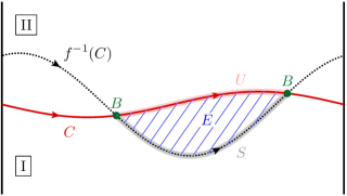
Figure 1: Partial barrier $C$ (red solid line) in a 2d cylindrical phase space and its preimage $f^{-1}(C)$ (black dotted line) confining the exit lobe $E$ (blue hatched) that is transported from region I to region II under the map $f$. The oriented boundary of $E$ is given by $\partial E=U-S$. The invariant points $B$ (dark green points) are the boundary of $U$ and also of $S$.

In the following we shortly review the notion of partial barriers and flux for a volume-preserving map $f$ acting on an $n$-dimensional phase space, see Ref. Mei2015 for an extended exposition. This will lead to the flux formula, Eq. (5), which will be applied to 2d and 4d maps in this paper.

A closed manifold $C$ of codimension one, i.e. with $(n-1)$ dimensions, divides phase space into two distinct regions, in the following referred to as region I and region II. This is illustrated in Fig. 1 for $n=2$ and a 1d manifold $C$. If the manifold $C$ is invariant under the map $f$, i.e. it is identical to its preimage $f{}^{-1}(C)$, it is a barrier to transport. If $C$ is not invariant, it acts as a partial barrier, since it allows for an exchange of phase-space volume from region I into II, and vice versa.

The flux $\Phi$ is the volume of phase space which is transported across the partial barrier, e.g. from region I to II, upon each iteration of the map $f$. The flux $\Phi$ can be determined from the partial barrier $C$ and its preimage $f^{-1}(C)$, see Fig. 1: Together both manifolds $C$ and $f$${}^{-1}(C)$ confine (several) $n$-dimensional volumes, denoted as lobes, located on opposite sides of the partial barrier $C$. The lobes located in region I are the exit set $E$ of region I, as points in $E$ are transported across $C$ into region II under one iteration of the map $f$. Thus the flux $\Phi$ across the partial barrier is given by the volume of $E$. Conversely, the lobes located in region II are the exit set of region II, as points in these lobes are transported across $C$ into region I under one iteration of the map $f$. We will restrict to the case of zero net flux across the partial barrier $C$, which holds for exact volume-preserving maps Mei2015 , i.e. the flux $\Phi$ also describes the identical phase-space volume transported from region II to I. The notion of a turnstile describes the combined action of the exit lobe of region I and the exit lobe of region II under iteration of the map $f$, which interchange phase-space volume between these regions like a rotating door KayMeiPer1984a ; Mei2015 .

The flux $\Phi$ across a partial barrier will be determined using differential forms, which allow for a convenient description independent of the number $n$ of phase-space dimensions Eas1991 ; LomMei2009 ; Mei2015 ,

$$\Phi=\int\limits_{E}\Omega=\int\limits_{E}\mathrm{d}\alpha=\int\limits_{\partial E}\alpha=\int\limits_{U}\alpha-\int\limits_{S}\alpha,$$ (1)

where $\Omega$ is a volume form that we assume to be exact, i.e. $\Omega=\mathrm{d}\alpha$, with $\alpha$ being some $(n-1)$-form. Stokes theorem is used in Eq. (1), such that the dimension of the integral is reduced by one. In the last step of Eq. (1) the boundary $\partial E$ of $E$ is decomposed, $\partial E=U-S$, into an oriented subset $U$ of the partial barrier, $U\subset C$, and an oriented subset $S$ of the preimage, $S\subset f^{-1}(C)$, see Fig. 1. The sets $U$ and $S$ are $(n-1)$-dimensional manifolds.

The restriction to an exact volume-preserving map $f$ with an $(n-1)$-form $\alpha$, allows to write LomMei2009 ; Mei2015

$$f^{*}\alpha-\alpha=\mathrm{d}\lambda,$$ (2)

where $f^{*}\alpha$ is the pullback and $\lambda$ is an $(n-2)$ form which is called the generating Lagrangian form. Using this for $\alpha$ in the last integral of Eq. (1) gives

$$\Phi=\int\limits_{U}\alpha-\int\limits_{S}(f^{*}\alpha-\mathrm{d}\lambda).$$ (3)

By applying Stokes theorem to the last term, using $\partial S=\partial U$, and by using $\int\limits_{S}f^{*}\alpha=\int\limits_{f(S)}\alpha$ one gets

$$\Phi=\int\limits_{\partial U}\lambda+\int\limits_{U}\alpha-\int\limits_{f(S)}\alpha.$$ (4)

Note that the iterated set $f(S)$ as well as $U$ are subsets of the partial barrier $C$. The $(n-2)$-dimensional boundary $\partial U$ of $U$ in Eq. (4) is also the boundary $\partial S$ of $S$. It is given by the intersection of the partial barrier and its preimage, $\partial U=\partial S=C\cap f^{-1}(C)$, see Fig. 1. In general one has several exit lobes of region I and then the sets $U$ and $S$ are composed of several pieces, which confine all exit lobes.

In this paper we consider $(n-1)$-dimensional partial barriers, which connect the $(n-2)$-dimensional elements of an invariant set $B$. Therefore the preimage of the partial barrier contains the same invariant set $B$, see Fig. 1. Thus the invariant set $B$ is a subset of the intersection of the partial barrier and its preimage, and thus $B\subset\partial U$. Additionally, we require that there are no further intersections, leading to $\partial U=B$. Note that this corresponds to hypothesis (H2) in Ref. Mei2015 .

Furthermore, for this class of partial barriers, the iterated set $f(S)\subset U$ appearing in Eq. (4) is, just like $S$, bounded by the invariant set $B$. Therefore $f(S)$ is in fact identical to the subset $U$. With $f(S)=U$ the last two integrals in Eq. (4) cancel, leading to LomMei2009 ; Mei2015

$$\Phi=\int\limits_{B}\lambda.$$ (5)

In the examples that will be studied in this paper, the invariant set $B$ consists of two parts which are each invariant. They occur at different ends of $U$ (for each lobe) and thus contribute with different signs to $B{}=\partial U$.

Remarkably, according to Eq. (5), the flux $\Phi$ across this class of partial barriers can be determined from the invariant set $B$ only. As a consequence, the flux $\Phi$ is independent of the specific choice of the partial barrier as long as it contains the invariant set $B$ and has no further intersections with its preimage. It allows for determining the $n$-dimensional flux by an $(n-2)$-dimensional integral over the invariant set $B$.

III Partial barriers and flux in 2d maps

In this section we apply the general formalism of partial barriers and flux, in particular Eq. (5), to symplectic 2d maps. By reviewing some aspects of the well-established theory of transport in 2d maps KayMeiPer1984b ; Mei1992 ; Mei2015 we introduce some notation needed for the generalization to symplectic 4d maps in Sec. IV. In particular, we consider partial barriers which are based on periodic orbits, as they allow to approximate the properties of a cantorus. Cantori give rise to the most restrictive partial barriers in 2d maps.

III.1 System

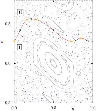
Figure 2: Phase space of the 2d standard map $f_{\textsc{2d}}$ for $K=1.75$ with regular tori (gray lines) and one chaotic orbit (blue points). A partial barrier (red solid line) separates region I and II. It is constructed by alternatingly joining the points of the periodic orbits $\bm{x}^{{2:5}}_{\text{max}}$ (dark green points) and $\bm{x}^{{2:5}}_{\text{min}}$ (light orange points).

As a paradigmatic example of a 2d map, we consider the standard mapChi1979 $f_{\textsc{2d}}$,

$$q^{\prime} =q+p$$ (6)

$$p^{\prime} =p-\frac{\mathrm{d}V}{\mathrm{d}q}(q^{\prime})$$

on the cylinder $(q,p)\in[0,1)\times\mathbb{R}$ with periodic boundary conditions imposed in $q$ and kicking potential $V(q)=\frac{K}{4\pi^{2}}\cos(2\pi q)$.

At kicking strength $K=0$ the mapping is integrable and the dynamics is foliated into rotational invariant 1d tori with fixed $p$. For $K>0$ tori with rational frequency break-up according to the Poincaré-Birkhoff theorem, while tori with sufficiently irrational frequency persist according to the KAM theorem LicLie1992 . These curves of codimension one form absolute barriers for chaotic transport in $p$-direction. The last rotational invariant torus breaks upGre1979 at $K_{c}\approx 0.97$. A mixed phase space for $K=1.75$ is shown in Fig. 2 where regions of regular and chaotic dynamics coexist. The chaotic region extends in the $p$-direction and transport is not blocked by any rotational invariant 1d torus. However, chaotic transport along the $p$-direction is impeded by the presence of 1d partial barriers. They are based on either periodic orbits or on cantori as invariant sets $B$, as discussed below.

III.2 Periodic orbits

We consider periodic orbits with frequency $\nu=\frac{m}{n}$, consisting of $n$ periodic points $\bm{x}^{{m:n}}_{{i}}=(q^{m:n}_{i},p^{m:n}_{i})$, $i=0,\dots,n-1$. Each point $\bm{x}^{{m:n}}_{{i}}$ is mapped to the next point, $f_{\textsc{2d}}(\bm{x}^{{m:n}}_{{i}})=\bm{x}^{{m:n}}_{{(i+1)\mod n}}$, and thus a fixed point of the $n$-fold map, $f_{\textsc{2d}}^{n}(\bm{x}^{{m:n}}_{{i}})=\bm{x}^{{m:n}}_{{i}}$. The index $m$ describes the number of cycles in $q$ after $n$ iterations. We denote the set of periodic points by

$$\bm{x}^{{m:n}}=\{\bm{x}^{{m:n}}_{{i}}\;|\;i=0,\dots,n-1\},$$ (7)

which is invariant under one iteration of the map,

$$f_{\textsc{2d}}(\bm{x}^{{m:n}})=\bm{x}^{{m:n}}.$$ (8)

These periodic orbits come in pairs, namely one so-called minimizing periodic orbit $\bm{x}^{{m:n}}_{\text{min}}$ and one minimax periodic orbit $\bm{x}^{{m:n}}_{\text{max}}$. Their existence is guaranteed by Aubry-Mather theory Mei1992 ; Mei2015 . For the considered kicking strength $K=1.75$ the periodic orbit $\bm{x}^{{2:5}}_{\text{min}}$ is hyperbolic and $\bm{x}^{{2:5}}_{\text{max}}$ is inverse hyperbolic, see Fig. 2.

III.3 Partial barriers based on periodic orbits

We consider partial barriers $C$ connecting points of the periodic orbits $\bm{x}^{{m:n}}_{\text{min}}$ and $\bm{x}^{{m:n}}_{\text{max}}$ in an alternating manner. One example of such a partial barrier $C$ is shown in Fig. 2, separating region I from II. It connects points of the periodic orbits $\bm{x}^{{2:5}}_{\text{min}}$ and $\bm{x}^{{2:5}}_{\text{max}}$. The preimage $f$${}^{-1}(C)$ intersects the partial barrier in the periodic points only, as shown in Fig. 3 (left). The partial barrier and its preimage enclose $2n$ lobes, which are alternatingly located above and below the partial barrier $C$. All lobes in region I contribute to the flux $\Phi$ to region II. Note that these criteria are fulfilled by infinitely many partial barriers, which turn out to all have the same flux.

In order to determine the flux across partial barriers of this kind we apply the flux formula, Eq. (5). Since the 2d standard map $f_{\textsc{2d}}$ is exact area-preserving with the one-form $\alpha=p\,\mathrm{d}q$, a generating zero-form (function) $\lambda_{\textsc{2d}}{}$ exists, given by

$$\lambda_{\textsc{2d}}{}=\frac{1}{2}p^{2}-V(q+p),$$ (9)

and fulfilling Eq. (2). The invariant set $B{}$ in the flux formula, Eq. (5), consists of $\bm{x}^{{m:n}}_{\text{max}}$ and $\bm{x}^{{m:n}}_{\text{min}}$ at the ends of $U$, contributing with different signs, $B{}=\bm{x}^{{m:n}}_{\text{max}}-\bm{x}^{{m:n}}_{\text{min}}$. This leads for the 2d case to the explicit expression BenKad1984 ; KayMeiPer1984b ; Mei1992 ; Mei2015

$$\Phi^{\textsc{2d}}=\int\limits_{B}\lambda_{\textsc{2d}}=\sum_{i=0}^{n-1}\>\lambda_{\textsc{2d}}(\bm{x}^{{m:n}}_{\text{max},{i}})\;-\;\sum_{i=0}^{n-1}\>\lambda_{\textsc{2d}}(\bm{x}^{{m:n}}_{\text{min},{i}}),$$ (10)

where integration reduces to a summation of the generating function evaluated on the pair of periodic orbits.

Note that the same flux is found for a partial barrier with a different construction giving just two lobes Mei1992 ; Mei2015 : One takes a piece of the above partial barrier, e.g., from one point of $\bm{x}^{{m:n}}_{\text{min}}$ to the neighboring point of $\bm{x}^{{m:n}}_{\text{min}}$ which goes through a point of $\bm{x}^{{m:n}}_{\text{max}}$. This curve is then iterated backwards $n-1$ times. Combining all these curves defines a partial barrier. Its preimage, by construction, is identical to the partial barrier, except for two lobes. The volume of the exit lobe, see Eq. (16) in Ref. Mei2015 , leads to the same flux Eq. (10).

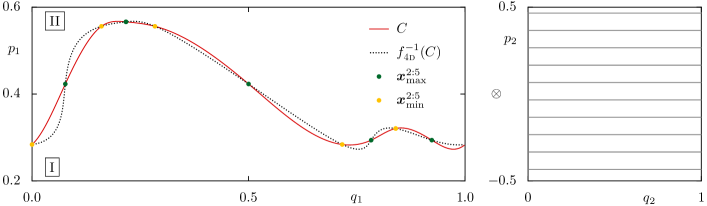
Figure 3: Product structure of the 4d standard map $f_{\textsc{4d}}$ without coupling $(\xi=0)$ for $K_{1}=1.75$, $K_{2}=0$. Periodic orbits $\bm{x}^{{2:5}}_{\text{max}}$ (dark green points) and $\bm{x}^{{2:5}}_{\text{min}}$ (light orange points) are shown in $(q_{1},p_{1})$ space. A partial barrier $C$ (red solid line) connects these periodic points and separates region I from region II. Its preimage $f_{\textsc{4d}}^{-1}(C)$ (black dotted line) intersects at the periodic points. Phase space in $(q_{2},p_{2})$ is integrable.

III.4 Cantorus

A cantorus Per1979 ; KayMeiPer1984b emerges when a 1d torus with irrational frequency $\nu$ breaks up under parameter variation. The remnants form a Cantor set. Such a cantorus can be successively approximated by the pair of periodic orbits, $\bm{x}^{{m:n}}_{\text{min}}$ and $\bm{x}^{{m:n}}_{\text{max}}$, with frequencies $\frac{m}{n}$ obtained by successive truncations of the continued fraction expansion of its irrational frequency $\nu$.

Partial barriers based on a cantorus are most restrictive for chaotic transport in 2d maps with locally the smallest flux. For the 2d standard map $f_{\textsc{2d}}$ the rotational invariant 1d torus with irrational frequency $\nu=1-\sigma_{\text{G}}\approx 0.382$, where $\sigma_{\text{G}}$ is the golden mean, persists longest with increasing $K$. It turns into a cantorus at the critical parameter $K_{c}\approx 0.97$ and has globally the smallest flux for $K>K_{c}$.

The flux $\Phi^{\textsc{2d}}$ of a partial barrier based on a cantorus can be successively approximated by the flux $\Phi^{\textsc{2d}}$, Eq. (10), of the pair of periodic orbits $\bm{x}^{{m:n}}_{\text{min}}$ and $\bm{x}^{{m:n}}_{\text{max}}$ with increasing periods $n$. Convergence of the flux is shown for $K=1.75$ in Fig. 5 and Tab. 1 where the flux $\Phi^{\textsc{2d}}$ is denoted as $\Phi^{\textsc{4d}}(\xi=0)$.

IV Partial barriers and flux in 4d maps

IV.1 Motivation

In a higher-dimensional phase space much less is known about partial barriers. A direct generalization from 2d maps is not possible. The reason is that invariant objects in phase space lack one or more dimensions in order to constitute a (partial) barrier. For example, in a 4d map a regular torus is a 2d manifold and thus cannot separate the 4d phase space into different regions. Consequently, also a broken 2d torus cannot form a restrictive partial barrier.

The existence of restrictive partial barriers in 4d maps, however, is indicated by numerical observations, see e.g. KanBag1985 ; MarDavEzr1987 ; Las1993 ; LanBaeKet2016 ; FirLanKetBae2018 . Their origin and their construction is still an open question.

In the following we introduce a 3d partial barrier in a 4d map based on higher-dimensional generalizations of the periodic orbits and cantori introduced in Sec. III. We will use the concept of normally hyperbolic invariant manifolds (NHIMs) Fen1972 ; HirPugShu1977 ; Man1978 ; Wig1994 ; Eld2013 to introduce a periodic NHIM and a cantorus-NHIM. The flux across partial barriers based on these invariant sets will be determined using Eq. (5).

IV.2 System

We consider the 4d standard mapFro1972 $f_{\textsc{4d}}$,

$$\begin{split}q_{1}^{\prime}&=q_{1}+p_{1}\\ q_{2}^{\prime}&=q_{2}+p_{2}\\ p_{1}^{\prime}&=p_{1}-V_{1}(q_{1}^{\prime},q_{2}^{\prime})\\ p_{2}^{\prime}&=p_{2}-V_{2}(q_{1}^{\prime},q_{2}^{\prime}),\end{split}$$ (11)

with the partial derivatives $V_{i}=\frac{\partial V(q_{1},q_{2})}{\partial q_{i}}$ and potential

$$\begin{split}V(q_{1},q_{2})=&\frac{K_{1}}{4\pi^{2}}\cos(2\pi{q_{1}})+\frac{K_{2}}{4\pi^{2}}\cos(2\pi{q_{2}})\\ &+\frac{\xi}{4\pi^{2}}\cos(2\pi{(q_{1}+q_{2})})\end{split}$$ (12)

composed of the potential of two 2d standard maps with kicking strengths $K_{1}$ and $K_{2}$ and a coupling between both degrees of freedom of strength $\xi$. We consider a cylinder in the first degree of freedom, $(q_{1},p_{1})\in[0,1)\times\mathbb{R}$, and a 2d torus in the second, $(q_{2},p_{2})\in[0,1)\times[-0.5,0.5)$ with periodic boundary conditions imposed in $q_{1},q_{2},p_{2}$.

Since we aim at a higher-dimensional partial barrier related to the cantorus of the 2d map, we fix $K_{1}=1.75$. Furthermore, for the occurrence of NHIMs (see discussion below) we require the kicking strength $K_{2}$ of the second degree of freedom to be much smaller than the kicking strength $K_{1}$ of the first degree of freedom, i.e. $K_{2}\ll K_{1}$. For simplicity we set $K_{2}=0$ throughout the paper.

If the coupling $\xi$ is set to zero, i.e. $\xi=0$, the 4d map $f_{\textsc{4d}}$ is trivially related to the 2d map $f_{\textsc{2d}}$. Phase-space structures are given by the Cartesian product of the objects in $(q_{1},p_{1})$ with the 2d torus of the $(q_{2},p_{2})$ space. This product structure is symbolically depicted in Fig. 3. As function of $p_{2}$ one obtains a stack of identical 2d maps in the $(q_{1},p_{1})$ space with rotational dynamics in $q_{2}$ whose frequency is given by $p_{2}$. In particular, any 1d partial barrier of the 2d map in the $(q_{1},p_{1})$ space trivially extends to a 3d partial barrier for the 4d map, see Sec. IV.4. Such a stack of systems has been used, e.g., in the famous Arnold model Arn1964 , its 4d map analogue EasMeiRob2001 , and in higher-dimensional scatteringJunMerSelZap2010 ; GonJun2012 ; GonDroJun2014 .

For non-zero but sufficiently small coupling strengths, ${\xi\ll 1}$, one obtains a 4d map with topological features of the product structure for $\xi=0$. This will be very helpful in visualizing phase-space structures and quantifying the flux across partial barriers.

IV.3 Periodic NHIMs

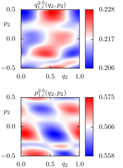
Figure 4: Parametrizations $q^{2:5}_{1,i}(q_{2},p_{2})$ and $p^{2:5}_{1,i}(q_{2},p_{2})$ of a 2d manifold, Eq. (15), of the periodic NHIM $\bm{X}_{\text{max},{}}^{{2:5}}$ for $\xi=0.05$ with $i$ corresponding to the periodic point with largest value of $p_{1}$. The corresponding periodic point of $f_{\textsc{2d}}$ is $(q,p)\approx(0.217,0.566)$. The projection of these parametrizations onto the $(q_{1},p_{1})$ space are shown in the inset of Fig. 7.

We introduce periodic NHIMs as the generalization of hyperbolic periodic orbits of the 2d map. If the coupling $\xi$ is set to zero, one obtains the Cartesian product of each hyperbolic periodic point $\bm{x}^{{m:n}}_{{i}}=(q^{m:n}_{i},p^{m:n}_{i})$ of $f_{\textsc{2d}}$ in $(q_{1},p_{1})$ space and the 2d torus of the $(q_{2},p_{2})$ space. This product structure is illustrated in Fig. 3. It gives rise to 2d manifolds $\bm{X}^{{m:n}}_{{i}}=\{(q_{i}^{m:n},p_{i}^{m:n},q_{2},p_{2})\;|\;q_{2}\in[0,1),p_{2}\in[-0.5,0.5)\}$ in the 4d phase space. Each of the manifolds $\bm{X}^{{m:n}}_{{i}}$ is mapped to the next manifold, $f_{\textsc{4d}}(\bm{X}^{{m:n}}_{{i}})=\bm{X}^{{m:n}}_{{(i+1)\mod n}}$, and is thus invariant under the $n$-fold map, $f_{\textsc{4d}}^{n}(\bm{X}^{{m:n}}_{{i}})=\bm{X}^{{m:n}}_{{i}}$. We denote this set of 2d manifolds by

$$\bm{X}^{{m:n}}=\{\bm{X}^{{m:n}}_{{i}}\;|\;i=0,\dots,n-1\},$$ (13)

which is invariant under one iteration of the map,

$$f_{\textsc{4d}}(\bm{X}^{{m:n}})=\bm{X}^{{m:n}}.$$ (14)

It is normally hyperbolic due to the underlying hyperbolic periodic orbit. We call $\bm{X}^{{m:n}}$ a periodic NHIM, as it is a NHIM that is build from a periodic set of manifolds.

These periodic NHIMs come in pairs, denoted by $\bm{X}_{\text{max}}^{{m:n}}$ and $\bm{X}_{\text{min}}^{{m:n}}$, as they emerge from the periodic orbits $\bm{x}^{{m:n}}_{\text{max}}$ and $\bm{x}^{{m:n}}_{\text{min}}$ of the map $f_{\textsc{2d}}$. It is required that the periodic orbit of $f_{\textsc{2d}}$ is hyperbolic or inverse hyperbolic. For approximants of the golden torus this is the case for $K_{1}>K_{c}\approx 0.97$ and sufficiently large period $n$. Specifically, for $K_{1}=1.75$ this is the case for $n\geq 3$. For an elliptic periodic orbit of $f_{\textsc{2d}}$, one cannot construct a periodic NHIM.

The case of small coupling, $\xi\ll 1$, can be considered as a small perturbation of the case without coupling such that the NHIMs persist. This is the case as long as the hyperbolicity in the normal directions is larger than in the tangential direction Fen1972 ; HirPugShu1977 ; Man1978 ; Wig1994 ; Eld2013 . Here it holds for ${K_{2}\ll K_{1}}$ and $\xi\ll 1$. The periodic NHIM for $\xi>0$ is no longer given by the trivial product structure. Instead, we parametrize the 2d manifolds by

$$\bm{X}^{{m:n}}_{{i}}=\{ \bigl{(}q^{m:n}_{1,i}(q_{2},p_{2}),p^{m:n}_{1,i}(q_{2},p_{2}),q_{2},p_{2}\bigr{)}\;|\;$$ (15)

$$q_{2}\in[0,1),\>p_{2}\in[-0.5,0.5)\},$$

for $i=0,\dots,n-1$. For $\xi\ll 1$ the parametrizations $q^{m:n}_{1,i}(q_{2},p_{2})$ and $p^{m:n}_{1,i}(q_{2},p_{2})$ are slightly varying around the coordinates of the periodic point $\bm{x}^{{m:n}}_{{i}}$ of $f_{\textsc{2d}}$. For an example this is visualized in Fig. 4. Numerically, we determine points on the periodic NHIMs by a binary contraction method BarJunFelMaiHer2018 (for an overview of methods see Ref. GonJun2022 ) taking into account the periodic structure Fir2020 .

Note that there is interesting dynamics on NHIMs LiShoTodKom2006a ; GuzLegFro2009b ; GonDroJun2014 ; GonJun2015 ; TerTodKom2015 ; CanHar2016 ; GonJun2022 . This also holds for periodic NHIMs and is presented for increasing periods in Appendix A.

IV.4 Partial barriers based on periodic NHIMs

We consider 3d partial barriers $C$ connecting the 2d manifolds of the periodic NHIMs $\bm{X}_{\text{min}}^{{m:n}}$ and $\bm{X}_{\text{max}}^{{m:n}}$ in an alternating manner, generalizing from the 2d map to the 4d map. Without coupling ($\xi=0$) a partial barrier is formed by the Cartesian product of a 1d partial barrier of the 2d map and the 2d torus of the $(q_{2},p_{2})$ space. It constitutes a 3d manifold dividing the 4d phase space. This product structure is illustrated in Fig. 3. The partial barrier and its preimage enclose $2n$ 4d lobe volumes, which are a Cartesian product of 2d lobes in the $(q_{1},p_{1})$ space and the 2d torus of the $(q_{2},p_{2})$ space, see Fig. 3.

In the presence of a small coupling, $\xi\ll 1$, the NHIMs persist and a slightly varied partial barrier $C$ can be constructed by connecting the NHIMs (in infinitely many ways). One has to ensure that the partial barrier and its preimage intersect in the periodic NHIMs only, i.e. $C\cap f_{\textsc{4d}}^{-1}(C)=\bm{X}_{\text{min}}^{{m:n}}{}\cup\bm{X}_{\text{max}}^{{m:n}}$.

In order to determine the flux across partial barriers of this kind we apply the flux formula, Eq. (5). Since the 4d standard map $f_{\textsc{4d}}$ is exact volume preserving with the three-form

$$\alpha=p_{1}\;\mathrm{d}q_{1}\wedge\mathrm{d}p_{2}\wedge\mathrm{d}q_{2}.$$ (16)

a generating two-form $\lambda_{\textsc{4d}}$ exists, given by

$$\lambda_{\textsc{4d}}=\Big{(}\frac{1}{2}p_{1}^{2}-V(q_{1}+p_{1},q_{2}+p_{2})\Big{)}\;\mathrm{d}p_{2}\wedge\mathrm{d}q_{2},$$ (17)

and fulfilling Eq. (2). The invariant set $B{}$ in the flux formula, Eq. (5), consists of $\bm{X}_{\text{max}}^{{m:n}}$ and $\bm{X}_{\text{min}}^{{m:n}}$ at the ends of $U$, contributing with different signs, $B{}=\bm{X}_{\text{max}}^{{m:n}}-\bm{X}_{\text{min}}^{{m:n}}$. This leads for the 4d case to the explicit expression

$$\Phi^{\textsc{4d}{}}=\int\limits_{B}\lambda_{\textsc{4d}}{}=\sum_{i=0}^{n-1}\int\limits_{\bm{X}_{\text{max},{i}}^{{m:n}}}\lambda_{\textsc{4d}}\;-\;\sum_{i=0}^{n-1}\int\limits_{\bm{X}_{\text{min},{i}}^{{m:n}}}\lambda_{\textsc{4d}}.$$ (18)

Let us stress, that the 4d flux across such a partial barrier is entirely determined by integrating a generating two-form $\lambda$ over the 2d manifolds of the periodic NHIMs. Thus the flux does not depend on the specific choice of partial barrier.

For the chosen three-form $\alpha$, Eq. (16), and the related generating two-form $\lambda_{\textsc{4d}}$, Eq. (17), just integrals with respect to the 2d torus of the $(q_{2},p_{2})$ space have to be determined. Numerically, one can use a grid in $(q_{2},p_{2})$ space and the parametrization of $\bm{X}^{{m:n}}$ from Eq. (15). The flux $\Phi^{\textsc{4d}}$ is determined for $\xi=0.05$ and various periods, see Fig. 5 and Tab. 1.

Note that without coupling, $\xi=0$, the evaluation of the flux formula, Eq. (18), simplifies, since the generating two-form $\lambda_{\textsc{4d}}$, Eq. (17), and the NHIMs become independent of $q_{2}$ and $p_{2}$. Consequently, the integration with respect to these coordinates simply yields $1$, i.e. the area of the 2d torus of the $(q_{2},p_{2})$ space. The remaining sum is equivalent to the flux formula for 2d maps, Eq. (10).

IV.5 Cantorus-NHIM

We now establish for 4d maps what we call a cantorus-NHIM. Without coupling, $\xi=0$, it is a Cartesian product of a cantorus with irrational frequency $\nu$ of the 2d map in $(q_{1},p_{1})$ space and the 2d torus of the $(q_{2},p_{2})$ space. It is normally hyperbolic due to the properties of the cantorus and it is invariant. We expect that this NHIM with a Cantor set structure persists for small coupling, $\xi\ll 1$, just like other NHIMs. It can be successively approximated by the pair of periodic NHIMs, $\bm{X}_{\text{min}}^{{m:n}}$ and $\bm{X}_{\text{max}}^{{m:n}}$, with frequencies $\frac{m}{n}$ obtained by successive truncations of the continued fraction expansion of the irrational frequency $\nu$.

The flux $\Phi^{\textsc{4d}}$ across a partial barrier based on a cantorus-NHIM is, in analogy to 2d maps, approximated by the flux $\Phi^{\textsc{4d}}$, Eq. (18), across partial barriers based on the pair of periodic NHIMs $\bm{X}_{\text{min}}^{{m:n}}$ and $\bm{X}_{\text{max}}^{{m:n}}$. Fast convergence of the flux $\Phi^{\textsc{4d}}$ with increasing periods $n$ is shown in Fig. 5 and Tab. 1 for $f_{\textsc{4d}}$ with $\xi=0.05$. The flux shows the same qualitative dependence on the period $n$ and is slightly larger than the flux without coupling $\Phi^{\textsc{4d}}(\xi=0)$, which corresponds to $\Phi^{\textsc{2d}}$ for $f_{\textsc{2d}}$.

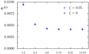
Figure 5: Flux $\Phi^{\textsc{4d}}$, Eq. (18), across partial barriers based on periodic NHIMs $\bm{X}^{{1:3}}$ to $\bm{X}^{{13:34}}$ for $\xi=0.05$ (crosses), converging to the flux across the cantorus-NHIM. It is compared to the flux $\Phi^{\textsc{4d}}(\xi=0)$ without coupling (circles) corresponding to $\Phi^{\textsc{2d}}$.

$m\!:\!n$	$\Phi^{\textsc{4d}}(\xi=0)$	$\Phi^{\textsc{4d}}(\xi=0.05)$
$1\!:\!3$	$0.0094004$	$0.0094771$
$2\!:\!5$	$0.0051837$	$0.0052659$
$3\!:\!8$	$0.0042684$	$0.0043532$
$5\!:\!13$	$0.0041162$	$0.0042000$
$8\!:\!21$	$0.0041104$	$0.0041941$
$13\!:\!34$	$0.0041104$	$0.0041941$

Table 1: Flux $\Phi^{\textsc{4d}}$, as displayed in Fig. 5, showing fast convergence with increasing period $n$.

We expect that these partial barriers based on a cantorus-NHIM are as important in 4d maps as their counterparts in 2d maps. This generalization to 4d maps should also apply to other cantori of the 2d map, e.g., originating from rotational 1d tori with different irrational frequency $\nu$ or from oscillatory 1d tori.

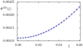
Figure 6: Flux $\Phi^{\textsc{4d}}$, Eq. (18), across partial barriers based on periodic NHIMs $\bm{X}^{{8:21}}$ vs. coupling $\xi$ (crosses), showing a quadratic increase (solid line).

We investigate the dependence of the flux $\Phi^{\textsc{4d}}$ on the coupling $\xi$ for the example of partial barriers based on the periodic NHIM $\bm{X}^{{8:21}}$, which closely approximates the flux across the cantorus-NHIM. In Fig. 6 the flux $\Phi^{\textsc{4d}}$ shows for $\xi\in[0.0,0.06]$ a quadratic increase, $\Phi^{\textsc{4d}}(\xi)\approx\Phi^{\textsc{4d}}(\xi=0)+0.0333\cdot\xi^{2}$. For other parameters $K_{1}$ and different periods we find also a quadratic dependence (not shown).

IV.6 4D lobe volume

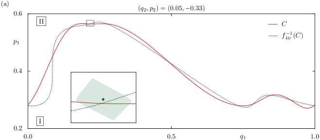
Figure 7: Example of a 3d partial barrier $C$ (red solid line) and its preimage $f_{\textsc{4d}}^{-1}(C)$ (black dotted line) in a $(q_{2},p_{2})$ section of phase space for (a) $(q_{2},p_{2})=(0.05,-0.33)$ and (b) $(q_{2},p_{2})=(0.39,-0.33)$, intersecting at periodic NHIMs $\bm{X}_{\text{min}}^{{2:5}}$ and $\bm{X}_{\text{max}}^{{2:5}}$ for $\xi=0.05$ and confining $5$ lobes each in region I and II. Insets: Magnification of one intersection together with the projection of $\bm{X}_{\text{max}}^{{2:5}}$ on the $(q_{1},p_{1})$ space (green colored area), see also Fig. 4, and the corresponding periodic point $\bm{x}^{{2:5}}_{\text{max}}$ of the 2d map (green point).

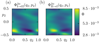
Figure 8: Flux (a) $\Phi^{\textsc{2d}}_{\text{I}\rightarrow\text{II}}$ and (b) $\Phi^{\textsc{2d}}_{\text{II}\rightarrow\text{I}}$ depending on the $(q_{2},p_{2})$ section for a 3d partial barrier based on the periodic NHIMs $\bm{X}^{{2:5}}$ for $\xi=0.05$.

Complementary to the evaluation of the flux formula, Eq. (18), we want to explicitly determine the 4d lobe volume for an example of a 3d partial barrier based on a periodic NHIM. This has several motivations: (i) it gives an independent verification of Eq. (18), (ii) it provides an impression of the geometry of the lobes, as for $\xi>0$ one no longer has a product structure, and (iii) it is a preparation for the determination of a local flux introduced and studied in Sec. V.

For convenience we consider 3d partial barriers that can be written as a function $p_{1}^{\text{pb}}(q_{1},q_{2},p_{2})$ of the three cyclic variables $(q_{1},q_{2},p_{2})$ of $f_{\textsc{4d}}$. This function can be expressed by a finite Fourier series. See Ref. Fir2020 for a construction, where a specific partial barrier is chosen by minimizing its curvature along the $q_{1}$ direction. One has to check numerically that the partial barrier and its preimage intersect in the periodic NHIMs only, i.e. $C\cap f_{\textsc{4d}}^{-1}(C)=\bm{X}_{\text{min}}^{{m:n}}{}\cup\bm{X}_{\text{max}}^{{m:n}}$.

As an example we choose a 3d partial barrier based on the periodic NHIMs $\bm{X}_{\text{min}}^{{2:5}}$ and $\bm{X}_{\text{max}}^{{2:5}}$. Sections for two exemplary fixed values of $(q_{2},p_{2})$ of the partial barrier and its preimage are shown in Fig. 7. In such a $(q_{2},p_{2})$ section the dimensionality of the objects is reduced by two, i.e. the partial barrier and its preimage appear as 1d lines. They confine 2d lobe areas, namely $5$ lobes in region I and $5$ lobes in region II with the same topology as in the uncoupled case, compare Fig. 3. The area of the individual lobes depends on the $(q_{2},p_{2})$ section, e.g., the area of the left-most lobe is bigger in Fig. 7(a) than in Fig. 7(b).

The sum of the lobe areas in region I in a given $(q_{2},p_{2})$ section gives the 2d flux to region II, denoted by $\Phi^{\textsc{2d}}_{\text{I}\rightarrow\text{II}}(q_{2},p_{2})$. The corresponding flux in the reverse direction is denoted by $\Phi^{\textsc{2d}}_{\text{II}\rightarrow\text{I}}(q_{2},p_{2})$. They are calculated according to Eq. (24) in Appendix B. Note, that under one iteration of the map $f_{\textsc{4d}}$ these lobe areas are no longer contained in the same $(q_{2},p_{2})$ section.

There is an asymmetry of this 2d flux for a given $(q_{2},p_{2})$ section. In Fig. 7(a) one can observe that the flux $\Phi^{\textsc{2d}}_{\text{I}\rightarrow\text{II}}(q_{2},p_{2})$ is greater than $\Phi^{\textsc{2d}}_{\text{II}\rightarrow\text{I}}(q_{2},p_{2})$, whereas in Fig. 7(b) it is the other way around. This is illustrated quantitatively in Fig. 8 for all sections $(q_{2},p_{2})$. Thus, one concludes that zero net flux does not hold for each $(q_{2},p_{2})$ section individually.

Finally, the 4d flux across the 3d partial barrier is obtained by integrating the 2d flux over all sections,

$$\Phi^{\textsc{4d}}=\iint\Phi^{\textsc{2d}}{}(q_{2},p_{2})\>\mathrm{d}q_{2}\>\mathrm{d}p_{2},$$ (19)

where it should be irrelevant whether $\Phi^{\textsc{2d}}_{\text{I}\rightarrow\text{II}}(q_{2},p_{2})$ or $\Phi^{\textsc{2d}}_{\text{II}\rightarrow\text{I}}(q_{2},p_{2})$ is integrated, as for the flux $\Phi^{\textsc{4d}}$ we have zero net flux, see Sec. II.

For a 3d partial barrier based on the periodic NHIMs $\bm{X}_{\text{min}}^{{2:5}}$ and $\bm{X}_{\text{max}}^{{2:5}}$ with $\xi=0.05$ we obtain, $\Phi^{\textsc{4d}}_{\text{I}\rightarrow\text{II}}=\Phi^{\textsc{4d}}_{\text{II}\rightarrow\text{I}}=0.0052659$. This result of the volume measurement of the 4d lobe volumes confirms the result $\Phi^{\textsc{4d}}=0.0052659$ of the flux formula, Eq. (18), see Tab. 1, entirely determined by the periodic NHIMs, within the numerical accuracy of the determination of the NHIMs.

IV.7 Partial barrier between resonance channels

We now discuss where the partial barriers studied in this paper are located in phase space and frequency space, in particular in comparison to resonance channels. This will be helpful for understanding more generic partial barriers, see the discussion in the outlook, Sec. VII. Quite importantly, it explains why the flux $\Phi^{\textsc{4d}}$ studied so far, will be considered as a global flux, in contrast to a local flux introduced in the next Sec. V.

We start with the important concept of resonances (for the 2d standard map) and resonance channels (for the 4d map). Resonances of a 2d map correspond to rational frequencies. For the 2d standard map at $K=0$ lines with rational $p$ break-up for $K>0$ into a chain of elliptic and hyperbolic periodic points together with surrounding regular tori and chaotic layer, respectively, to form a so-called resonance. The two most prominent resonances have frequency $\nu=0$ at $p=0$ and $\nu=\frac{1}{2}$ at $p=0.5$, see Fig. 2. The corresponding elliptic points are surrounded by a regular island and the hyperbolic points are embedded in a chaotic layer. Transport between these chaotic layers is possible for $K>K_{c}$. It is limited by the partial barrier with the smallest flux between the resonances $\nu=0$ and $\nu=\frac{1}{2}$ which is based on the golden cantorus with $\nu\approx 0.382$, see Sec. III.

For a 4d map the 2d regular tori are characterized by two frequencies $(\nu_{1},\nu_{2})$. A pair of frequencies is called resonant if it fulfills $m_{1}\nu_{1}+m_{2}\nu_{2}=k$ with integers $m_{1},m_{2},k$. In frequency space they form so-called resonance lines, denoted by $m_{1}:m_{2}:k$. In phase space the corresponding objects constitute a resonance channel which consists of families of 2d tori, families of elliptic 1d tori and hyperbolic 1d tori, together with their surrounding chaotic motion, seeOnkLanKetBae2016 for an illustration of a generic resonance channel of a 4d map.

For the 4d map with $K_{1}>0$ and $K_{2}=0$ and small coupling the resonances of $f_{\textsc{2d}}$ for $\nu=0$ and $\nu=\frac{1}{2}$ lead to the $1:0:0$ resonance line and the $2:0:1$ resonance line, with frequencies $\nu_{1}=0$ and $\nu_{1}=\frac{1}{2}$, respectively, while $\nu_{2}\in[-0.5,0.5)$ extends along the entire $\nu_{2}$ axis. These resonance lines are thus both parallel to the $\nu_{2}$ axis in frequency space. In phase space, both resonance lines correspond to resonance channels extending in $p_{2}$ direction. For $K_{1}>K_{c}$ transport across a partial barrier between these resonances is possible for $f_{\textsc{2d}}$ and therefore also across a partial barrier between the corresponding resonance channels for $f_{\textsc{4d}}$. The flux between these resonance channels is restricted by the cantorus-NHIM, as studied in Sec. IV. It gives rise to a partial barrier extended between the ${1:0:0}$ and ${2:0:1}$ resonance lines in frequency space, such that $\nu_{1}=1-\sigma_{\text{G}}$ and $\nu_{2}$ is extended along the entire $\nu_{2}$-axis. This corresponds in phase space to the entire $p_{2}$-axis with $p_{2}\in[-0.5,0.5)$. The flux $\Phi^{\textsc{4d}}$ across the cantorus-NHIM from resonance channel ${1:0:0}$ to resonance channel ${2:0:1}$ is thus a global flux.

Note that partial barriers associated with irrational frequency lines have been proposed in Ref. MarDavEzr1987 . To our knowledge, the partial barrier based on the cantorus-NHIM is the first explicit realization.

V Local Flux in 4d maps

V.1 Motivation

Resonance channels, introduced in IV.7, play a prominent role for chaotic transport in 4d symplectic maps. Transport along a resonance channel is often slow due to Arnold diffusion Arn1964 ; Chi1979 ; Loc1999 ; Dum2014 . Transport from one resonance channel to another may occur at so-called resonance junctionsHal1995 ; Hal1999 ; GotNoz1999 ; Got2006 ; EftHar2013 ; KarKes2018 . Here we are interested in transport between (nearly) parallel resonance channels restricted by a partial barrier in between the resonance channels. Due to the slow transport along a resonance channel, the local properties of the partial barrier at a given position along the resonance channel are important. Typically, these local properties will be more relevant than the global flux accumulated along the entire resonance channel. We will therefore introduce a local flux, that depends on the position along a resonance channel.

Specifically, for the 4d standard map $f_{\textsc{4d}}$ with $K_{2}=0$ and small coupling $\xi\ll 1$, transport in the $p_{2}$-direction is rather slow. This is the case as the change in $p_{2}$ is proportional to the coupling $\xi$, see Eqs. (11) and (12). The dynamics in $q_{1}$ and $q_{2}$ is much faster. Also transitions in $p_{1}$ from the ${1:0:0}$ resonance channel to the ${2:0:1}$ resonance channel via a partial barrier may occur many times, while the $p_{2}$ coordinate barely changes.

Thus, in order to describe chaotic transport more precisely, one needs to know the local flux near a given $p_{2}$ coordinate along the resonance channel, rather than the global flux $\Phi^{\textsc{4d}}$. To this end we use a $p_{2}$-section of the 4d lobe volume to define the local 3d flux $\Phi^{\textsc{3d}}(p_{2})$ across a partial barrier. It can be determined based on the area of the lobe in $(q_{2},p_{2})$ sections, $\Phi^{\textsc{2d}}_{\text{I}\rightarrow\text{II}}(q_{2},p_{2})$ or $\Phi^{\textsc{2d}}_{\text{II}\rightarrow\text{I}}(q_{2},p_{2})$, as introduced in IV.6. By integrating over $q_{2}$ one finds the local flux,

$$\Phi^{\textsc{3d}}(p_{2})=\int\mathrm{d}q_{2}\>\Phi^{\textsc{2d}}(q_{2},p_{2}),$$ (20)

which differs from Eq. (19) as there is no integration along $p_{2}$. As an aside, we mention that the local flux $\Phi^{\textsc{3d}}(p_{2})$ divided by the 3d volume of the resonance channel at the given $p_{2}$ coordinate gives an estimate for the local transition rate across the partial barrier.

Note that for $f_{\textsc{4d}}$ without coupling, $\xi=0$, the flux $\Phi^{\textsc{2d}}(q_{2},p_{2})$ does not depend on $q_{2}$ and $p_{2}$, due to the product structure, see Fig. 3. Therefore the integration over $q_{2}\in[0,1)$ in Eq. (20) simply gives a factor of $1$ and the local flux $\Phi^{\textsc{3d}}$ does not depend on $p_{2}$ in this case, leading to the same values for $\Phi^{\textsc{3d}}(\xi=0)$ and $\Phi^{\textsc{4d}}(\xi=0)$.

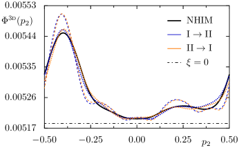
Figure 9: Local flux $\Phi^{\textsc{3d}}(p_{2})$, Eq. (20), for two different 3d partial barriers (dotted and dashed thin lines) and both directions $\text{I}\rightarrow\text{II}$ (dark blue) and $\text{II}\rightarrow\text{I}$ (light orange) based on the peridic NHIM $\bm{X}^{{2:5}}$ for coupling $\xi=0.05$. Comparison to the local flux without coupling, $\Phi^{\textsc{3d}}(\xi=0)$ (black dash-dotted line) and to the NHIM contribution, $\Phi^{\textsc{3d}}_{\text{NHIM}}(p_{2})$, Eq. (30) (black thick line).

V.2 Dependence on partial barrier

For a given periodic NHIM or cantorus-NHIM the global flux $\Phi^{\textsc{4d}}$ is independent of a specific partial barrier, see Sec. IV. Moreover, the net flux is zero across any partial barrier for the considered exact volume preserving maps. Here, we investigate whether the local flux $\Phi^{\textsc{3d}}(p_{2})$, Eq. (20), depends on specific partial barriers and examine whether zero net flux holds locally. Furthermore, we want to study how the local flux depends on $p_{2}$.

To this end we consider two (arbitrary) examples of partial barriers. The first was already utilized in Sec. IV.6. The second partial barrier is defined by requiring a specific slope of the partial barrier at the periodic NHIMs in addition to minimizing its curvature along the $q_{1}$ direction Fir2020 . The lobe areas in the $(q_{2},p_{2})$ sections differ substantially and one obtains a different flux $\Phi^{\textsc{2d}}(q_{2},p_{2})$ than in Fig. 8 (not shown). We checked that the global flux $\Phi^{\textsc{4d}}$ is indeed the same as before.

In Fig. 9 we show the local flux $\Phi^{\textsc{3d}}(p_{2})$ from region I to region II and vice versa for both partial barriers. This allows to draw several conclusions on the local flux $\Phi^{\textsc{3d}}(p_{2})$: (i) it depends on $p_{2}$, (ii) it depends on the partial barrier, and (iii) it weakly depends on the direction ($\text{I}{}\to\text{II}{}$ vs. $\text{II}{}\to\text{I}{}$), i.e. there is no zero net flux in a given $p_{2}$ section.

Quite importantly, Fig. 9 exhibits also common features of the local flux $\Phi^{\textsc{3d}}(p_{2})$. For both partial barriers and both directions we find a prominent maximum at $p_{2}\approx-0.4$ and a minimum at $p_{2}\approx 0$ (with larger values than without coupling, $\xi=0$, for all $p_{2}$). This will be further studied below.

Note that the definition of a local flux $\Phi^{\textsc{3d}}(p_{2})$ can be done in various ways. In Eq. (20) the $p_{2}$ section of exit lobes is used. Alternatively, one could take the $p_{2}$ section of the iterated exit lobes. In this case we find qualitatively similar, but quantitatively different results.

V.3 NHIM contribution

The local flux, although depending on specific partial barriers, shares common features, as shown in Fig. 9. Common to both partial barriers is, that they are based on the same periodic NHIM. Thus, it is plausible that these common features are related to the underlying periodic NHIM.

We propose a splitting of the local flux $\Phi^{\textsc{3d}}(p_{2})$ into two contributions,

$$\Phi^{\textsc{3d}}(p_{2})=\Phi^{\textsc{3d}}_{\text{NHIM}}(p_{2})+\delta_{\text{pb}}(p_{2}),$$ (21)

where the first term $\Phi^{\textsc{3d}}_{\text{NHIM}}(p_{2})$, defined in Eq. (30) in Appendix C, is entirely based on the periodic NHIM. We thus call it the NHIM contribution. The remaining term, $\delta_{\text{pb}}(p_{2}):=\Phi^{\textsc{3d}}(p_{2})-\Phi^{\textsc{3d}}_{\text{NHIM}}(p_{2})$, describes the deviations from the NHIM contribution, i.e. the additional $p_{2}$ dependence specific for the considered partial barrier.

The NHIM contribution, $\Phi^{\textsc{3d}}_{\text{NHIM}}(p_{2})$, is shown in Fig. 9 and it captures the common features of the $p_{2}$ dependence of the local flux $\Phi^{\textsc{3d}}(p_{2})$ quite well. We find that the local flux of partial barriers based on NHIMs with longer periods and varying parameters $(K_{1},\xi)$, are also well captured by the NHIM contribution (not shown). For a different class of partial barrier we also find good agreement, as discussed below in Sec. VI.4. We thus conjecture, that the $p_{2}$ dependence of the local flux $\Phi^{\textsc{3d}}(p_{2})$, Eq. (20), is in general well described by the NHIM contribution, $\Phi^{\textsc{3d}}_{\text{NHIM}}(p_{2})$, Eq. (30).

Numerically, we find that integrating over $p_{2}$ of the NHIM contribution yields the global flux $\Phi^{\textsc{4d}}{}$, $\int\mathrm{d}p_{2}\>\Phi^{\textsc{3d}}_{\text{NHIM}}(p_{2})=\Phi^{\textsc{4d}}{}$, as well as cancellation of the barrier-specific contribution, $\int\mathrm{d}p_{2}\>\delta_{\text{pb}}(p_{2})=0$. Both results are found up to the numerical precision of the NHIMs and we expect them to hold exactly.

V.4 Cantorus-NHIM

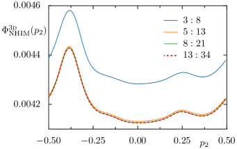
Figure 10: NHIM contribution $\Phi^{\textsc{3d}}_{\textsc{NHIM}}(p_{2})$, Eq. (30), to the local flux for periodic NHIMs $\bm{X}^{{3:8}}$ to $\bm{X}^{{13:34}}$ (top to bottom) for coupling $\xi=0.05$.

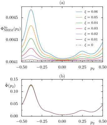
Figure 11: (a) Dependence of the NHIM contribution $\Phi^{\textsc{3d}}_{\textsc{NHIM}}(p_{2})$, Eq. (30), on the coupling $\xi$ for the periodic NHIM $\bm{X}^{{8:21}}$ for $\xi\in\{0.01,\cdots,0.06\}$ (solid lines from bottom to top) and flux $\Phi^{\textsc{3d}}(\xi=0)$ without coupling (dash-dotted line). (b) Quadratically scaled flux $\tilde{\Phi}(p_{2})=[\Phi^{\textsc{3d}}_{\textsc{NHIM}}{}-\Phi^{\textsc{3d}}(\xi=0)]/\xi^{2}$.

For a partial barrier based on a cantorus-NHIM the local flux $\Phi^{\textsc{3d}}(p_{2})$ is approximated by the NHIM contribution, $\Phi^{\textsc{3d}}_{\text{NHIM}}(p_{2})$, across partial barriers based on the pair of periodic NHIMs, $\bm{X}_{\text{min}}^{{m:n}}$ and $\bm{X}_{\text{max}}^{{m:n}}$, with frequencies $\frac{m}{n}$ converging to the frequency of the cantorus-NHIM. We are interested in the convergence of the $p_{2}$ dependence, which is presented in Fig. 10. Fast convergence of $\Phi^{\textsc{3d}}_{\textsc{NHIM}}(p_{2})$ with increasing periods $n$ can be observed. As for $\frac{2}{5}$ in Fig. 9, we find for other frequencies $\frac{m}{n}$ a prominent peak located at $p_{2}\approx-\frac{m}{n}$, converging towards $p_{2}=\sigma_{\text{G}}-1$, and a minimum at $p_{2}\approx 0$. We observe that the prominent peak occurs at the $p_{2}$ value, where the dynamics on the NHIM shows the biggest resonance, see Fig. 14 in Appendix A. This is at a crossing of the $1:1:0$ resonance channel with the cantorus-NHIM.

In Sec. IV.5 a quadratic dependence of the global flux $\Phi^{\textsc{4d}}$ on the coupling $\xi$ is observed. Here we study this dependence for the NHIM contribution $\Phi^{\textsc{3d}}_{\textsc{NHIM}}(p_{2})$ of the local flux, again for the periodic NHIM $\bm{X}^{{8:21}}$, which closely approximates the flux across the cantorus-NHIM.

In Fig. 11(a) we observe qualitatively that for all couplings $\xi$ the NHIM contribution has roughly the same $p_{2}$ dependence, but with increasing amplitude and increasing average. We quadratically scale the difference of the NHIM contribution $\Phi^{\textsc{3d}}_{\textsc{NHIM}}(p_{2})$ to the flux without coupling, i.e. we divide the difference by $\xi^{2}$. One observes in Fig. 11(b) that the curves almost coincide. The remaining small variations indicate some higher-order contribution of the small coupling $\xi\ll 1$.

VI Partial barrier from 3d stable and unstable manifolds of a NHIM

VI.1 Motivation

In 2d maps there is another important partial barrier besides the partial barrier based on a cantorus. It arises from a 0d hyperbolic fixed (or periodic) point and its 1d stable and unstable manifolds Mei1992 ; Mei2015 . One can generalize this partial barrier to the case of a 4d map by considering the 2d NHIM related to the hyperbolic fixed point and its 3d stable and unstable manifolds Wig1990 ; GilEzr1991 . We want to demonstrate that the flux $\Phi^{\textsc{4d}}{}$ across this partial barrier composed of 3d stable and unstable manifolds can be determined by the flux across appropriate periodic NHIMs. This approach is similar to 2d maps Mei1992 , where the flux across a partial barrier composed of stable and unstable manifolds of a periodic orbit with frequency $\frac{m}{n}$ can be determined by increasingly higher-order periodic orbits with frequencies converging to $\frac{m}{n}$.

Furthermore we want to study the local flux $\Phi^{\textsc{3d}}(p_{2})$ for this partial barrier. In particular, we want to test if the NHIM contribution captures the prominent features of the $p_{2}$ dependence of the local flux also for this type of partial barrier, which is composed of invariant manifolds.

As an aside, we mention that one can avoid the determination of NHIMs by constructing corresponding 2d manifolds by interpolating families of 1d hyperbolic tori Hue2020 . This gives approximately the same global and local flux, but becomes less accurate for increasing coupling, as the dynamics on the NHIMs has larger resonances and chaotic regions (see Fig. 14 in the appendix).

VI.2 Partial barrier and flux

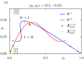
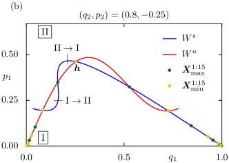
Figure 12: Partial barrier composed of segments of the 3d stable ($W^{\text{s}}$) and unstable ($W^{\text{u}}$) manifolds of the 2d NHIM $\bm{X}_{\text{min}}^{{0:1}}$ merging at the 2d homoclinic manifold $\bm{h}$ in a $(q_{2},p_{2})$ section of phase space for (a) $(q_{2},p_{2})=(0.3,-0.25)$ and (b) $(q_{2},p_{2})=(0.8,-0.35)$ for $\xi=0.05$. Exit lobes from region I and from region II are shown. Periodic NHIMs $\bm{X}_{\text{max}}^{{1:15}}$ (dark green points) and $\bm{X}_{\text{min}}^{{1:15}}$ (light orange points) approximate the intersections of stable and unstable manifolds.

We consider the 4d map $f_{\textsc{4d}}$ with parameters as in Sec. IV.2. The 2d NHIM $\bm{X}_{\text{min}}^{{0:1}}$ corresponds to the hyperbolic fixed point $\bm{x}^{{0:1}}_{\text{min}}=(0,0)$ of the 2d map $f_{\textsc{2d}}$. This NHIM has a 3d stable manifold $W^{\text{s}}$ and a 3d unstable manifold $W^{\text{u}}$. The manifolds $W^{\text{s}}$ and $W^{\text{u}}$ intersect (infinitely often) in 2d homoclinic manifolds. This is shown for two $(q_{2},p_{2})$ sections of the 4d phase space in Fig. 12, where the 3d manifolds appear as 1d lines intersecting in 0d points.

The 3d partial barrier is composed of segments of $W^{\text{s}}$ and $W^{\text{u}}$ ranging from the NHIM $\bm{X}_{\text{min}}^{{0:1}}$ to a specific chosen homoclinic manifold $\bm{h}$, see Fig. 12. It separates phase space into regions I and II. There is one 4d exit lobe from region I and one exit lobe from region II, each enclosed by segments of the stable and unstable manifolds. For this exact volume preserving map they lead to the same global flux $\Phi^{\textsc{4d}}$. These lobes appear as 2d areas in the $(q_{2},p_{2})$ sections of Fig. 12 of varying sizes. The global flux $\Phi^{\textsc{4d}}$ for $\xi=0.05$ is determined by integrating the 2d areas over all $(q_{2},p_{2})$ sections, giving $\Phi^{\textsc{4d}}=0.0064679$ for each lobe.

VI.3 Flux from periodic NHIMs

$m\!:\!n$	$\Phi^{\textsc{4d}}(\xi=0)$	$\Phi^{\textsc{4d}}(\xi=0.05)$
$1\!:\!3$	$0.0094004$	$0.0094771$
$1\!:\!5$	$0.0066441$	$0.0067190$
$1\!:\!7$	$0.0064130$	$0.0064891$
$1\!:\!9$	$0.0063935$	$0.0064697$
$1\!:\!11$	$0.0063918$	$0.0064680$
$1\!:\!13$	$0.0063917$	$0.0064679$
$1\!:\!15$	$0.0063917$	$0.0064679$

Table 2: Flux $\Phi^{\textsc{4d}}$, Eq. (18), across partial barriers based on periodic NHIMs $\bm{X}^{{1:3}}$ to $\bm{X}^{{1:15}}$ for coupling $\xi=0$ and $\xi=0.05$, showing fast convergence with increasing period $n$.

In 2d maps one can use periodic orbits to determine the flux across a partial barrier composed of stable and unstable manifolds. This is possible as appropriate periodic orbits approximate the homoclinic intersections of stable and unstable manifolds. There is a flux formula based on these (infinitely many) homoclinic intersections Mei1992 . These ideas have been generalized to arbitrary dimensions LomMei2009 ; Mei2015 .

We want to use periodic NHIMs, introduced in IV.3, to determine the global flux $\Phi^{\textsc{4d}}{}$ across a partial barrier composed of 3d stable and unstable manifolds. This has the advantage that it does not require the numerical determination of 3d stable and unstable manifolds and their 2d homoclinic intersections.

We use periodic NHIMs $\bm{X}_{\text{max}}^{{1:n}}$ and $\bm{X}_{\text{min}}^{{1:n}}$ with frequencies $\nu=\frac{1}{n}$ for increasing $n$. They appear as 0d periodic points in the $(q_{2},p_{2})$ sections of Fig. 12, where they approximate several homoclinic intersections of the stable and unstable manifolds of the NHIM $\bm{X}_{\text{min}}^{{0:1}}$. The flux $\Phi^{\textsc{4d}}{}$ across periodic NHIMs is determined using Eq. (18). It converges for increasing $n$, as shown in Tab. 2, agreeing with the above 4d volume measurement of the exit lobe. Note that the flux for this type of partial barrier is about $50\%$ larger than for the cantorus-NHIM for the considered parameters, see Tab. 1, as is the case for the 2d map $f_{\textsc{2d}}$. This also quantitatively confirms that the cantorus-NHIM provides the more restrictive transport barrier.

VI.4 Local flux

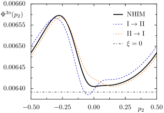
Figure 13: Local flux $\Phi^{\textsc{3d}}(p_{2})$, Eq. (20), for the 3d partial barrier composed of segments of the 3d stable and unstable manifolds of the 2d NHIM $\bm{X}_{\text{min}}^{{0:1}}$ in direction $\text{I}\rightarrow\text{II}$ (dark blue dashed line) and $\text{II}\rightarrow\text{I}$ (light orange dashed line) based on the periodic NHIM $\bm{X}^{{1:15}}$ for coupling $\xi=0.05$. Comparison to the local flux without coupling, $\Phi^{\textsc{3d}}(\xi=0)$ (black dash-dotted line) and to the NHIM contribution, $\Phi^{\textsc{3d}}_{\text{NHIM}}(p_{2})$, Eq. (30) (black thick line).

We study the local flux $\Phi^{\textsc{3d}}(p_{2})$ for the partial barrier composed of segments of the 3d stable and unstable manifolds of the 2d NHIM $\bm{X}_{\text{min}}^{{0:1}}$. To this end, we determine the local flux from region I to region II and vice versa, by integrating the 2d areas in the $(q_{2},p_{2})$ sections with respect to $q_{2}$, Eq. (20). The result for the local flux $\Phi^{\textsc{3d}}(p_{2})$ is depicted in Fig. 13, showing the $p_{2}$-dependence for this kind of partial barrier and a weak dependence on the direction showing that there is no zero net flux in a given $p_{2}$ section.

We find that the NHIM contribution $\Phi^{\textsc{3d}}_{\textsc{NHIM}}(p_{2})$ captures the prominent features of the $p_{2}$ dependence of the local flux also for this type of partial barrier, see Fig. 13. Here the partial barrier is defined by naturally occurring invariant manifolds, in contrast to Sec. V, where infinitely many partial barriers joining the NHIMs could be used. This shows that the NHIM contribution for the local flux gives the most important contribution, both for the partial barrier based on the cantorus NHIM and for partial barriers from 3d stable and unstable manifolds of a NHIM.

Note that one can study other partial barriers, by using a different homoclinic manifold than $\bm{h}$, where stable and unstable manifolds are joined, see Fig. 12. For example, one could use $f_{\textsc{4d}}(\bm{h})$ further to the right or $f_{\textsc{4d}}^{-1}(\bm{h})$ further to the left. In these cases we find that the deviation of the local flux from the NHIM contribution is larger, but also the difference between the local flux in the two directions is increased Fir2020 .

VII Summary and outlook

For 4d symplectic maps we propose a partial barrier based on the new concept of a cantorus-NHIM. To determine the flux across such a partial barrier we establish the relevance of periodic NHIMs consisting of $n$ 2d manifolds. These generalize the 0d periodic orbits, which are crucial for the approximation of a cantorus in 2d symplectic maps. We determine the 4d flux $\Phi^{\textsc{4d}}$, Eq. (18), across a partial barrier based on a pair of periodic NHIMs. The flux can be determined directly from the 2d manifolds of the periodic NHIMs. We check this approach by comparing with explicit volume measurements of the 4d lobe volumes. By increasing the periodicity, while approximating with $\frac{m}{n}$ an irrational frequency, these periodic NHIMs approximate a cantorus NHIM and the 4d flux converges.

In the presence of slow Arnold diffusion along a resonance channel the global 4d flux for the entire resonance channel gives limited information. Therefore we introduce the more relevant local 3d flux, depending on the position along a resonance channel. This local 3d flux turns out to depend on the specific choice of the partial barrier even when based on the same pair of periodic NHIMs. The relevant common features of the dependence on the position along the resonance channel, however, are very well described by a NHIM-dependent contribution $\Phi^{\textsc{3d}}_{\text{NHIM}}(p_{2})$, Eq. (30). This allows for describing the local flux from one resonance channel to another resonance channel independent of a specific partial barrier and just based on the 2d manifolds of a pair of periodic NHIMs.

Finally, we utilize periodic NHIMs to quantify the flux across a partial barrier composed of stable and unstable manifolds of a NHIM, both for the global 4d flux and the local 3d flux. This answers a question raised in Ref. Mei2015 , Question IV (Multidimensional Flux). Can one use the flux formulas to compute flux […] through resonance zones formed from 2d normally hyperbolic invariant sets in a 4d symplectic map […]?, in the affirmative.

The present work opens the path for the analysis of more generic situations in 4d symplectic maps. Here, we rely on a parameter regime for which the NHIMs emerge from an uncoupled case. When increasing the coupling strength the hyperbolicity on the NHIMs increases and will eventually lead to a breakup of the NHIMs GonDroJun2014 ; TerTodKom2015 ; Jun2021 . If just part of the NHIM exists, the assumptions of Sec. II are not fulfilled and a global 4d flux can no longer be determined. However, a local 3d flux may still be well defined.

Furthermore, the partial barriers studied here are in frequency space all parallel to a frequency axis and they are in between parallel resonance channels. Generically, one has transport between resonance channels that are not parallel to a frequency axis and that are not parallel to each other, as observed e.g. in Refs. MarDavEzr1987 ; Las1993 ; LanBaeKet2016 ; FirLanKetBae2018 . Still we expect that periodic NHIMs occur and can be used to determine the local flux. We expect that such a local flux from one resonance channel to another will depend much stronger on the position along the resonance channel than in the examples studied here. In particular, we expect the local flux to be small near a predominantly regular region and to increase towards the chaotic sea. Understanding this local flux will give new insights in finding the mechanism of stickiness leading to power-law trapping in higher-dimensional systems LanBaeKet2016 .

Moreover, the partial barriers based on periodic NHIMs can be directly generalized to higher-dimensional symplectic maps with weakly coupled degrees of freedom. In case of an $n$-dimensional map the corresponding NHIMs consist of $(n-2)$-dimensional manifolds. An $(n-1)$-dimensional partial barrier based on them will allow for an $n$-dimensional flux. The flux can be determined in analogy to Eq. (18) from the properties of a pair of periodic NHIMs only. The ideas presented here should also be relevant and applicable to higher-dimensional time-continuous systems and transition state theory in particular.

Finally, consequences of a partial barrier on the corresponding quantum system are of interest. It is known from the lower-dimensional case that the flux across a partial barrier has to be compared to the size of a Planck cell KayMeiPer1984b ; MicBaeKetStoTom2012 ; KoeBaeKet2015 : If the Planck cell is larger than the flux one finds that quantum mechanically transport is blocked, while in the opposite case classical transport is mimicked. The transition is described by a universal scaling curve. It is an interesting question to find out the relevant scaling in the higher-dimensional case. Presumably, the ratio of 4d flux to 4d Planck cell is relevant. But it is not clear, if this ratio enters the universal scaling curve or its square root, which describes the ratio per degree of freedom. This question becomes even more relevant in higher dimensions. Additionally, it will be worth exploring the quantum mechanical impact of a strongly varying local 3d flux.

Appendix A Dynamics on 2D periodic NHIMs

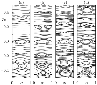
Figure 14: Phase-space structures on the 2d periodic NHIM $\bm{X}_{\text{max}}^{{m:n}}$ at $K_{1}=1.75$, $K_{2}=0$, $\xi=0.03$ for frequencies $\frac{m}{n}\in\{\frac{1}{3},\frac{2}{5},\frac{3}{8},\frac{5}{13}\}$ from (a) to (d), visualized by a projection of the manifold with $q_{1}\approx 0.5$ onto $(q_{2},p_{2})$ space.

Each of the $n$ manifolds $\bm{X}^{{m:n}}_{{i}}$ of a periodic NHIM $\bm{X}^{{m:n}}$ is invariant under the $n$-fold map, $f_{\textsc{4d}}^{n}(\bm{X}^{{m:n}}_{{i}})=\bm{X}^{{m:n}}_{{i}}$, for $i=0,\dots,n-1$. Therefore one can study the dynamics of the $n$-fold 4d map $f_{\textsc{4d}}^{n}$ restricted to one of the 2d manifolds $\bm{X}^{{m:n}}_{{i}}$. This is visualized in Fig. 14 for the periodic NHIM $\bm{X}_{\text{max}}^{{m:n}}$ for increasing periods $n$ with $\frac{m}{n}$ approaching the golden mean. Such phase-space portraits for NHIMs based on hyperbolic fixed points (i.e. with period $n=1$) have been studied in Refs. LiShoTodKom2006a ; GonDroJun2014 ; GonJun2015 ; TerTodKom2015 ; CanHar2016 ; GonJun2022 .

Without coupling, $\xi=0$, one finds integrable dynamics for $K_{2}=0$, as shown in Fig. 3 (right). A small coupling effectively acts as perturbation leading to resonances and chaotic layers, as in a non-integrable 2d symplectic map, see Fig. 14. With increasing coupling the size of the resonances and the associated chaotic layers increase Fir2020 .

The occurring resonances on the manifold are related to the frequency $\frac{m}{n}$ of the NHIM $\bm{X}^{{m:n}}$. They occur at so-called resonance junctionsHal1995 ; Hal1999 ; GotNoz1999 ; Got2006 ; EftHar2013 ; KarKes2018 in frequency space, where the resonance line ${n:0:m}$ intersects with the periodic NHIM. The biggest resonance (at $p_{2}=-\frac{m}{n}$) appears at the crossing with the ${1:1:0}$ resonance channel. The second biggest resonance (at $p_{2}=0$) occurs at the crossing with the ${0:1:0}$ resonance channel.

We mention that the phase-space portraits of all manifolds $\bm{X}^{{m:n}}_{{i}}$ with $i=0,\dots,n-1$ show qualitatively the same phase-space structure with some shift in $q_{2}$-direction. The phase-space portraits of $\bm{X}_{\text{min}}^{{m:n}}$ (not shown) do not differ substantially from the ones shown for $\bm{X}_{\text{max}}^{{m:n}}$ in Fig. 14.

Numerically, one has to deal with the instability of the dynamics normal to the periodic NHIM. Thus after each iteration of the map $f_{\textsc{4d}}$, Eq. (11), we project the 4d orbit onto the corresponding manifold $\bm{X}^{{m:n}}_{{i}}$. This is done by using the iterated $(q_{2},p_{2})$ coordinates and determining the corresponding $(q_{1},p_{1})$ coordinates of the NHIM using the parametrization, Eq. (15).

Appendix B Flux $\Phi^{\textsc{2D}}$ in $(q_{2},p_{2})$ section

A 3d partial barrier $C$ and its 3d preimage $f_{\textsc{4d}}^{-1}(C)$ give rise to 4d lobe volumes transported from region I to II. For the computation of this 4d volume in Eq. (19) we use an integral over $(q_{2},p_{2})$ sections of phase space. The objects in such a section appear in the remaining $(q_{1},p_{1})$ space with a dimension reduced by two. Here the partial barrier and its preimage are 1d lines, see Fig. 7. Together they enclose 2d lobe areas which vary with the considered $(q_{2},p_{2})$ section.

The sum of the lobe areas in region I gives the flux $\Phi^{\textsc{2d}}_{\text{I}\rightarrow\text{II}}(q_{2},p_{2})$ for a chosen $(q_{2},p_{2})$ section. This flux can be directly evaluated from Eq. (4) by considering the $(q_{2},p_{2})$ sections of the 3d manifolds $U$ and $S$, giving the 1d manifolds $U_{q_{2},p_{2}}$ and $S_{q_{2},p_{2}}$, respectively. Let us remind, that $U$ and $S$ enclose the exit set, see Fig. 1 for $n=2$, and $U$ is a subset of the partial barrier $C$, while $S$ is a subset of the preimage, such that $f_{\textsc{4d}}{}(S)$ is also a subset of $C$. In contrast to $f_{\textsc{4d}}{}(S)=U$ used for the derivation of Eq. (5), for the here considered $(q_{2},p_{2})$ section we have $f_{\textsc{4d}}{}(S_{q_{2},p_{2}})\neq U_{q_{2},p_{2}}$ and the last two integrals in Eq. (4) do not cancel. This leads for the map $f_{\textsc{4d}}$ with the generating two-form $\lambda_{\textsc{4d}}$, Eq. (17), to

$$\Phi^{\textsc{2d}}_{\text{I}\rightarrow\text{II}}(q_{2},p_{2})= \int\limits_{\partial U_{q_{2},p_{2}}}\frac{1}{2}p_{1}^{2}-V(q_{1}+p_{1},q_{2}+p_{2})$$ (22)

$$+\int\limits_{U_{q_{2},p_{2}}}p_{1}\>\mathrm{d}q_{1}-\int\limits_{f_{\textsc{4d}}(S_{q_{2},p_{2}})}p_{1}\>\mathrm{d}q_{1}.$$

The 0d boundary points $\partial U_{q_{2},p_{2}}$ are on the pair of periodic NHIMs, $\bm{X}_{\text{min}}^{{m:n}}$ and $\bm{X}_{\text{max}}^{{m:n}}$, which are on the left (L) and on the right (R) end of the $i$-th lobe, respectively,

$$\bm{x}_{i}^{\text{L/R}}=(q_{1,i}^{\text{L/R}}(q_{2},p_{2}),p_{1,i}^{\text{L/R}}(q_{2},p_{2}),q_{2},p_{2}),$$ (23)

for $i=0,\dots,n-1$. Here the $(q_{1},p_{1})$ coordinates depend on the considered $(q_{2},p_{2})$ section according to the parametrization of the NHIMs, Eq. (15).

For the iterated set $f_{\textsc{4d}}(S_{q_{2},p_{2}})$ we use the mapping, Eq. (11). For a 3d partial barrier, $p_{1}^{\text{pb}}(q_{1},q_{2},p_{2})$, we find for the flux $\Phi^{\textsc{2d}}$ in a $(q_{2},p_{2})$ section the explicit expression

$$\Phi^{\textsc{2d}}_{\text{I}\rightarrow\text{II}}(q_{2},p_{2})= \sum_{i=0}^{n-1}\>\left[\frac{1}{2}p_{1}^{2}-V(q_{1}+p_{1},q_{2}+p_{2})\right]^{\bm{x}_{i}^{\text{R}}}_{\bm{x}_{i}^{\text{L}}}$$ (24)

$$+\sum_{i=0}^{n-1}\>\int\limits_{q_{1,i}^{\text{L}}}^{q_{1,i}^{\text{R}}}p_{1}^{\text{pb}}(q_{1},q_{2},p_{2})\>\mathrm{d}q_{1}$$

$$-\sum_{i=0}^{n-1}\>\int\limits_{q_{1,i}^{\text{L}}+p_{1,i}^{\text{L}}}^{q_{1,i}^{\text{R}}+p_{1,i}^{\text{R}}}p_{1}^{\text{pb}}(q_{1},q_{2}^{\prime},p_{2}^{\prime})\>\mathrm{d}q_{1},$$

with $q_{2}^{\prime}=q_{2}+p_{2}$ and $p_{2}^{\prime}=p_{2}-V_{2}(q_{1},q_{2}+p_{2})$ according to Eq. (11).

In order to compute the flux $\Phi^{\textsc{2d}}_{\text{II}\rightarrow\text{I}}$ for the opposite transport direction, the other set of lobe areas have to be considered. This is done by interchanging the role of the left and right NHIM in Eq. (24) and increasing the index $i$ for the right NHIM by one. Additionally, the overall sign has to be changed to get a positive flux $\Phi^{\textsc{2d}}_{\text{II}\rightarrow\text{I}}$.

Appendix C NHIM contribution to local flux $\Phi^{\textsc{3D}}(p2)$

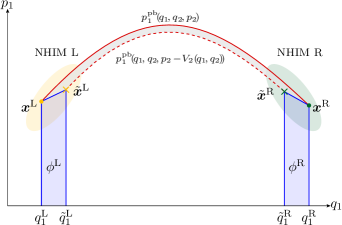
Figure 15: Visualization of integrands appearing in Eq. (25). Partial barrier $C$ for fixed $(q_{2},p_{2})$ in $(q_{1},p_{1})$ space, $p_{1}^{\text{pb}}(q_{1},q_{2},p_{2})$ (red solid line), between endpoints $\bm{x}^{\text{L/R}}$ (light orange and dark green point) on left and right NHIM (ellipsoidal shaded areas). Partial barrier $C$ at different $p_{2}$ coordinate, $p_{1}^{\text{pb}}(q_{1},q_{2},p_{2}-V_{2}(q_{1},q_{2}))$ (red dashed line), between endpoints $\tilde{\bm{x}}^{\text{L/R}}$ (light orange and dark green cross). The difference of areas under the curves is shaded and consists of the trapezoidal NHIM-dependent areas $\phi^{\text{L/R}}$ (blue) and the barrier-specific area (gray).

We derive the splitting of the local flux $\Phi^{\textsc{3d}}(p_{2})$, Eq. (21), into the NHIM contribution $\Phi^{\textsc{3d}}_{\text{NHIM}}(p_{2})$ and the barrier-specific contribution $\delta_{\text{pb}}(p_{2})$. Starting point is Eq. (20), where the flux $\Phi^{\textsc{2d}}(q_{2},p_{2})$, Eq. (24), is inserted,

$$\begin{split}&\Phi^{\textsc{3d}}{}(p_{2})=\int\limits_{0}^{1}\mathrm{d}q_{2}\\ &\quad\begin{aligned} \times\Bigg{(}\;&\sum_{i=0}^{n-1}\>\left[\frac{1}{2}p_{1}^{2}-V(q_{1}+p_{1},q_{2}+p_{2})\right]^{\bm{x}_{i}^{\text{R}}}_{\bm{x}_{i}^{\text{L}}}\\ &+\sum_{i=0}^{n-1}\>\int\limits_{q_{1,i}^{\text{L}}}^{q_{1,i}^{\text{R}}}p_{1}^{\text{pb}}(q_{1},q_{2},p_{2})\>\mathrm{d}q_{1}\\ {}&-\sum_{i=0}^{n-1}\>\int\limits_{\tilde{q}^{\text{L}}_{1,i}}^{\tilde{q}^{\text{R}}_{1,i}}p_{1}^{\text{pb}}\big{(}q_{1},q_{2},p_{2}-V_{2}(q_{1},q_{2})\big{)}\>\mathrm{d}q_{1}\Bigg{)}.\end{aligned}\end{split}$$ (25)

In the last line the integration variable $q_{2}$ is changed to $q_{2}^{\prime}=q_{2}+p_{2}$ and the periodicity in $q_{2}$ is used with the prime omitted afterwards. This change of variables has the advantage that now both integrands of the last two lines have the same $q_{2}$ coordinate and for the considered small coupling almost the same $p_{2}$ coordinate, such that the difference of the integrals is small, as used below.

Moreover, in the last line of Eq. (25) we use the coordinates $\tilde{q}^{\text{L/R}}_{1,i}$ of the points

$$\tilde{\bm{x}}_{i}^{\text{L/R}}=f_{\textsc{4d}}\big{(}\bm{x}_{i-1}^{\text{L/R}}(q_{2}-p_{2},p_{2})\big{)},$$ (26)

marked by a tilde, which are the iterates of the boundary points $\partial S_{q_{2}-p_{2},p_{2}}=\partial U_{q_{2}-p_{2},p_{2}}$ on the NHIMs, where the index $i$ of the NHIM manifold is changed by one, such that the points $\tilde{\bm{x}}_{i}^{\text{L/R}}$ are near the corresponding points $\bm{x}_{i}^{\text{L/R}}$, Eq. (23). In terms of coordinates we have

$$\tilde{\bm{x}}_{i}^{\text{L/R}} =\big{(}\tilde{q}_{1,i}^{\text{L/R}},\tilde{p}_{1,i}^{\text{L/R}},q_{2},p_{2}-V_{2}(\tilde{q}^{\text{L/R}}_{1,i},q_{2})\big{)},$$ (27)

with the $\tilde{q}^{\text{L/R}}_{1,i}$ and $\tilde{p}^{\text{L/R}}_{1,i}$ determined according to Eq. (26) using Eq. (11),

$$\tilde{q}^{\text{L/R}}_{1,i} =q_{1,i-1}^{\text{L/R}}(q_{2}-p_{2},p_{2})+p_{1,i-1}^{\text{L/R}}(q_{2}-p_{2},p_{2}),$$ (28)

$$\tilde{p}^{\text{L/R}}_{1,i} =p_{1,i-1}^{\text{L/R}}(q_{2}-p_{2},p_{2})-V_{1}(\tilde{q}^{\text{L/R}}_{i,1},q_{2}).$$

These points $\tilde{\bm{x}}_{i}^{\text{L/R}}$ are by construction on the left and the right NHIM, respectively, but in contrast to the points $\bm{x}_{i}^{\text{L/R}}$, Eq. (23), have a slightly different $p_{2}$ coordinate.

The first term in Eq. (25) depends on properties of the NHIMs only. It is similar to Eq. (18), up to the missing integration with respect to $p_{2}$. One expects that this term describes the dominant features of the local flux. However, this term alone is insufficient to describe the local flux as we find that it varies as a function of $p_{2}$ on a roughly 10 times larger scale (not shown) compared to the local flux $\Phi^{\textsc{3d}}(p_{2})$ in Fig. 9.

Thus also the last two lines of Eq. (25) have to be considered to find the relevant contribution of the local flux $\Phi^{\textsc{3d}}(p_{2})$, which depends on the NHIMs only. A sketch of these integrals (without $q_{2}$ integration and without summation over $i$) is shown in Fig. 15 in the $(q_{1},p_{1})$ space for fixed $(q_{2},p_{2})$. Specifically, both integrands and their integration limits are sketched. For the local flux, Eq. (25), the small difference of these integrals is relevant, shown by transparently colored areas.

There are two blue colored parts of this area, which depend on the NHIMs only, denoted as $\phi_{i}^{\text{L/R}}$. These contributions are within the intervals $[q_{1,i}^{\text{L}},\tilde{q}_{1,i}^{\text{L}}]$ and $[\tilde{q}_{1,i}^{\text{R}},q_{1,i}^{\text{R}}]$, respectively, and originate from the different integration limits in Eq. (25). For the upper boundary of the areas $\phi_{i}^{\text{L/R}}$ we choose a straight line connecting the points $\bm{x}_{i}^{\text{L/R}}$ and $\tilde{\bm{x}}_{i}^{\text{L/R}}$ on the left and the right NHIM, respectively, projected onto $(q_{1},p_{1})$ space (other choices are discussed below). The trapezoidal areas $\phi_{i}^{\text{L/R}}$ are given by

$$\phi_{i}^{\text{L/R}}=\left(q_{1,i}^{\text{L/R}}-\tilde{q}_{1,i}^{\text{L/R}}\right)\;\frac{p_{1,i}^{\text{L/R}}+\tilde{p}_{1,i}^{\text{L/R}}}{2}\;.$$ (29)

We include these two NHIM-dependent areas to define the NHIM contribution of the local flux, Eq. (25),

$$\begin{split}&\Phi^{\textsc{3d}}_{\text{NHIM}}(p_{2})=\\ &\quad\begin{aligned} \int\limits_{0}^{1}\mathrm{d}q_{2}\Bigg{(}\;&\sum_{i=0}^{n-1}\>\left[\frac{1}{2}p_{1}^{2}-V(q_{1}+p_{1},q_{2}+p_{2})\right]^{\bm{x}_{i}^{\text{R}}(q_{2},p_{2})}_{\bm{x}_{i}^{\text{L}}(q_{2},p_{2})}\\ &+\sum_{i=0}^{n-1}\left[\phi_{i}^{\text{R}}(q_{2},p_{2})-\phi_{i}^{\text{L}}(q_{2},p_{2})\right]\Bigg{)}.\end{aligned}\end{split}$$ (30)

The remaining term, $\delta_{\text{pb}}(p_{2}):=\Phi^{\textsc{3d}}(p_{2})-\Phi^{\textsc{3d}}_{\text{NHIM}}(p_{2})$, describes the deviations from the NHIM contribution, i.e. the additional $p_{2}$ dependence specific for the considered partial barrier. It is related to the gray colored area in Fig. 15.

We mention as an aside, that the straight connection between the points $\bm{x}_{i}^{\text{L/R}}$ and $\tilde{\bm{x}}_{i}^{\text{L/R}}$ used above is not part of the NHIMs. Thus another conceptual interesting way is to connect the points by a path which is entirely on the NHIMs Fir2020 . Since the results do not change significantly, this is not further discussed here.

References

- (1) P. Schlagheck and A. Buchleitner, Algebraic decay of the survival probability in chaotic helium, Phys. Rev. A 63, 024701 (2001).
- (2) S. Wiggins, L. Wiesenfeld, C. Jaffé, and T. Uzer, Impenetrable barriers in phase-space, Phys. Rev. Lett. 86, 5478–5481 (2001).
- (3) M. Toda, T. Komatsuzaki, T. Konishi, R. S. Berry, and S. A. Rice (editors) Geometric Structures of Phase Space in Multidimensional Chaos: Applications to Chemical Reaction Dynamics in Complex Systems, volume 130 of Advances in Chemical Physics, John Wiley & Sons, Inc., Hoboken, New Jersey (2005).
- (4) S. Gekle, J. Main, T. Bartsch, and T. Uzer, Extracting multidimensional phase space topology from periodic orbits, Phys. Rev. Lett. 97, 104101 (2006).
- (5) R. Paškauskas, C. Chandre, and T. Uzer, Dynamical bottlenecks to intramolecular energy flow, Phys. Rev. Lett. 100, 083001 (2008).
- (6) H. Waalkens, R. Schubert, and S. Wiggins, Wigner’s dynamical transition state theory in phase space: classical and quantum, Nonlinearity 21, R1–R118 (2008).
- (7) P. Manikandan and S. Keshavamurthy, Intramolecular vibrational energy redistribution from a high frequency mode in the presence of an internal rotor: Classical thick-layer diffusion and quantum localization, J. Chem. Phys. 127, 064303 (2007).
- (8) P. Manikandan and S. Keshavamurthy, Dynamical traps lead to the slowing down of intramolecular vibrational energy flow, Proc. Natl. Acad. Sci. USA 111, 14354–14359 (2014).
- (9) N. Murray and M. Holman, The role of chaotic resonances in the Solar System, Nature 410, 773–779 (2001).
- (10) P. M. Cincotta, Arnold diffusion: an overview through dynamical astronomy, New Astron. Rev. 46, 13–39 (2002).
- (11) J. Daquin, A. J. Rosengren, E. M. Alessi, F. Deleflie, G. B. Valsecchi, and A. Rossi, The dynamical structure of the MEO region: long-term stability, chaos, and transport, Celest. Mech. Dyn. Astron. 124, 335–366 (2016).
- (12) C. Jaffé, S. D. Ross, M. W. Lo, J. Marsden, D. Farrelly, and T. Uzer, Statistical theory of asteroid escape rates, Phys. Rev. Lett. 89, 011101 (2002).
- (13) J. Daquin, I. Gkolias, and A. J. Rosengren, Drift and its mediation in terrestrial orbits, Front. Appl. Math. Stat. 4, 35 (2018).
- (14) I. Gkolias, J. Daquin, D. K. Skoulidou, K. Tsiganis, and C. Efthymiopoulos, Chaotic transport of navigation satellites, Chaos 29, 101106 (2019).
- (15) H. S. Dumas and J. Laskar, Global dynamics and long-time stability in Hamiltonian systems via numerical frequency analysis, Phys. Rev. Lett. 70, 2975–2979 (1993).
- (16) M. N. Vrahatis, H. Isliker, and T. C. Bountis, Structure and breakdown of invariant tori in a 4-D mapping model of accelerator dynamics, Int. J. Bifurcation Chaos 7, 2707–2722 (1997).
- (17) Y. Papaphilippou, Detecting chaos in particle accelerators through the frequency map analysis method, Chaos 24, 024412 (2014).
- (18) R. S. MacKay, J. D. Meiss, and I. C. Percival, Stochasticity and transport in Hamiltonian systems, Phys. Rev. Lett. 52, 697–700 (1984).
- (19) R. S. MacKay, J. D. Meiss, and I. C. Percival, Transport in Hamiltonian systems, Physica D 13, 55–81 (1984).
- (20) J. D. Meiss, Symplectic maps, variational principles, and transport, Rev. Mod. Phys. 64, 795–848 (1992).
- (21) J. D. Meiss, Thirty years of turnstiles and transport, Chaos 25, 097602 (2015).
- (22) D. G. Truhlar, B. C. Garrett, and S. J. Klippenstein, Current status of transition-state theory, J. Phys. Chem. 100, 12771–12800 (1996).
- (23) H. Waalkens and S. Wiggins, Direct construction of a dividing surface of minimal flux for multi-degree-of-freedom systems that cannot be recrossed, J. Phys. A 37, L435–L445 (2004).
- (24) H. Waalkens and S. Wiggins, Geometrical models of the phase space structures governing reaction dynamics, Regul. Chaotic Dyn. 15, 1–39 (2010).
- (25) R. S. MacKay and D. C. Strub, Bifurcations of transition states: Morse bifurcations, Nonlinearity 27, 859–895 (2014).
- (26) G. S. Ezra and S. Wiggins, Sampling phase space dividing surfaces constructed from normally hyperbolic invariant manifolds (NHIMs), J. Phys. Chem. A 122, 8354–8362 (2018).
- (27) A. J. Lichtenberg and M. A. Lieberman, Regular and Chaotic Dynamics, Springer–Verlag, New York, second edition (1992).
- (28) I. C. Percival, Variational principles for invariant tori and cantori, in AIP Conference Proceedings, volume 57, 302–310, AIP Publishing (1979).
- (29) H. E. Lomelí and J. D. Meiss, Resonance zones and lobe volumes for exact volume-preserving maps, Nonlinearity 22, 1761–1789 (2009).
- (30) A. M. Fox and R. de la Llave, Barriers to transport and mixing in volume-preserving maps with nonzero flux, Physica D 295–296, 1–10 (2015).
- (31) A. M. Fox and J. D. Meiss, Greene’s residue criterion for the breakup of invariant tori of volume-preserving maps, Physica D 243, 45–63 (2013).
- (32) A. M. Fox and J. D. Meiss, Computing the conjugacy of invariant tori for volume-preserving maps, SIAM J. Appl. Dyn. Syst. 15, 557–579 (2016).
- (33) S. Das and A. Bäcker, Power-law trapping in the volume-preserving Arnold-Beltrami-Childress map, Phys. Rev. E 101, 032201 (2020).
- (34) B. V. Chirikov, A universal instability of many-dimensional oscillator systems, Phys. Rep. 52, 263–379 (1979).
- (35) J. Tennyson, Resonance transport in near-integrable systems with many degrees of freedom, Physica D 5, 123–135 (1982).
- (36) B. P. Wood, A. J. Lichtenberg, and M. A. Lieberman, Arnold diffusion in weakly coupled standard maps, Phys. Rev. A 42, 5885–5893 (1990).
- (37) G. Haller, Chaos Near Resonance, number 138 in Applied Mathematical Sciences, Springer New York (1999).
- (38) P. M. Cincotta, C. M. Giordano, and C. Simó, Phase space structure of multi-dimensional systems by means of the mean exponential growth factor of nearby orbits, Physica D 182, 151–178 (2003).
- (39) S. Honjo and K. Kaneko, Structure of Resonances and Transport in Multi-dimensional Hamiltonian Dynamical Systems, in Toda et al. TodKomKonBerRic2005 , chapter 22, 437–463.
- (40) P. M. Cincotta, C. Efthymiopoulos, C. M. Giordano, and M. F. Mestre, Chirikov and Nekhoroshev diffusion estimates: Bridging the two sides of the river, Physica D 266, 49–64 (2014).
- (41) F. Onken, S. Lange, R. Ketzmerick, and A. Bäcker, Bifurcations of families of 1D-tori in 4D symplectic maps, Chaos 26, 063124 (2016).
- (42) S. Lange, A. Bäcker, and R. Ketzmerick, What is the mechanism of power-law distributed Poincaré recurrences in higher-dimensional systems?, EPL 116, 30002 (2016).
- (43) V. I. Arnol’d, Instability of dynamical systems with several degrees of freedom, Sov. Math. Dokl. 5, 581–585 (1964).
- (44) P. Lochak, Arnold diffusion; A compendium of remarks and questions, in C. Simó (editor) Hamiltonian Systems with Three or More Degrees of Freedom, volume 533 of NATO ASI Series: C - Mathematical and Physical Sciences, 168–183, Kluwer Academic Publishers, Dordrecht (1999).
- (45) H. S. Dumas, The KAM Story: A Friendly Introduction to the Content, History, and Significance of Classical Kolmogorov–Arnold–Moser Theory, World Scientific, Singapore (2014).
- (46) N. Fenichel, Persistence and smoothness of invariant manifolds for flows, Indiana Univ. Math. J. 21, 193–226 (1972).
- (47) M. W. Hirsch, C. C. Pugh, and M. Shub, Invariant Manifolds, number 583 in Lect. Notes Math., Springer Berlin Heidelberg (1977).
- (48) R. Mañé, Persistent manifolds are normally hyperbolic, Trans. Amer. Math. Soc. 246, 261–283 (1978).
- (49) S. Wiggins, Normally hyperbolic invariant manifolds in dynamical systems, Springer–Verlag, Berlin (1994).
- (50) J. Eldering, Normally Hyperbolic Invariant Manifolds, number 2 in Atlantis Series in Dynamical Systems, Atlantis Press, Paris (2013).
- (51) K. Kaneko and R. J. Bagley, Arnold diffusion, ergodicity, and intermittency in coupled standard mapping, Phys. Lett. A 110, 435–440 (1985).
- (52) C. C. Martens, M. J. Davis, and G. S. Ezra, Local frequency analysis of chaotic motion in multidimensional systems: Energy transport and bottlenecks in planar OCS, Chem. Phys. Lett. 142, 519–528 (1987).
- (53) J. Laskar, Frequency analysis for multi-dimensional systems. Global dynamics and diffusion, Physica D 67, 257–281 (1993).
- (54) M. Firmbach, S. Lange, R. Ketzmerick, and A. Bäcker, Three-dimensional billiards: Visualization of regular structures and trapping of chaotic trajectories, Phys. Rev. E 98, 022214 (2018).
- (55) Video corresponding to Fig. 7 of FirLanKetBae2018 .
- (56) S. Wiggins, On the geometry of transport in phase space I. Transport in -degree-of-freedom Hamiltonian systems, , Physica D 44, 471–501 (1990).
- (57) R. E. Gillilan and G. S. Ezra, Transport and turnstiles in multidimensional Hamiltonian mappings for unimolecular fragmentation: Application to van der Waals predissociation, J. Chem. Phys. 94, 2648–2668 (1991).
- (58) Q. Chen, R. S. MacKay, and J. D. Meiss, Cantori for symplectic maps, J. Phys. A 23, L1093–L1100 (1990).
- (59) E. M. Bolt and J. D. Meiss, Breakup of invariant tori for the four-dimensional semi-standard map, Physica D 66, 282–297 (1993).
- (60) R. W. Easton, Transport through chaos, Nonlinearity 4, 583–590 (1991).
- (61) J. M. Greene, A method for determining a stochastic transition, J. Math. Phys. 20, 1183–1201 (1979).
- (62) D. Bensimon and L. P. Kadanoff, Extended chaos and disappearance of KAM trajectories, Physica D 13, 82–89 (1984).
- (63) C. Froeschlé, Numerical study of a four-dimensional mapping, Astron. & Astrophys. 16, 172–189 (1972).
- (64) R. W. Easton, J. D. Meiss, and G. Roberts, Drift by coupling to an anti-integrable limit, Physica D 156, 201–218 (2001).
- (65) C. Jung, O. Merlo, T. H. Seligman, and W. P. K. Zapfe, The chaotic set and the cross section for chaotic scattering in three degrees of freedom, New J. Phys. 12, 103021 (2010).
- (66) F. Gonzalez and C. Jung, Rainbow singularities in the doubly differential cross section for scattering off a perturbed magnetic dipole, J. Phys. A 45, 265102 (2012).
- (67) F. Gonzalez, G. Drotos, and C. Jung, The decay of a normally hyperbolic invariant manifold to dust in a three degrees of freedom scattering system, J. Phys. A 47, 045101 (2014).
- (68) R. Bardakcioglu, A. Junginger, M. Feldmaier, J. Main, and R. Hernandez, Binary contraction method for the construction of time-dependent dividing surfaces in driven chemical reactions, Phys. Rev. E 98, 032204 (2018).
- (69) F. Gonzalez Montoya and C. Jung, The numerical search for the internal dynamics of NHIMs and their pictorial representation, Physica D 436, 133330 (2022).
- (70) M. Firmbach, Chaotic transport and partial barriers in 4D symplectic maps, Ph.D. thesis, Technische Universität Dresden, Fakultät Physik (2020).
- (71) C.-B. Li, A. Shoujiguchi, M. Toda, and T. Komatsuzaki, Definability of no-return transition states in the high-energy regime above the reaction threshold, Phys. Rev. Lett. 97, 028302 (2006).
- (72) M. Guzzo, E. Lega, and C. Froeschlé, A numerical study of the topology of normally hyperbolic invariant manifolds supporting arnold diffusion in quasi-integrable systems, Physica D 238, 1797–1807 (2009).
- (73) F. Gonzalez and C. Jung, Visualizing the perturbation of partial integrability, J. Phys. A 48, 435101 (2015).
- (74) H. Teramoto, M. Toda, and T. Komatsuzaki, Breakdown mechanisms of normally hyperbolic invariant manifolds in terms of unstable periodic orbits and homoclinic/heteroclinic orbits in Hamiltonian systems, Nonlinearity 28, 2677–2698 (2015).
- (75) M. Canadell and À. Haro, A Newton-like method for computing normally hyperbolic invariant tori, in À. Haro, M. Canadell, J.-L. Figueras, A. Luque, and J. M. Mondelo (editors) The Parameterization Method for Invariant Manifolds: From Rigorous Results to Effective Computations, Applied Mathematical Sciences, 187–238, Springer International Publishing, Cham (2016).
- (76) G. Haller, Diffusion at intersecting resonances in hamiltonian systems, Phys. Lett. A 200, 34–42 (1995).
- (77) S.-i. Goto and K. Nozaki, Dynamics near resonance junctions in hamiltonian systems, Progr. Theor. Phys. 102, 937–946 (1999).
- (78) S.-i. Goto, Analytical expression for low-dimensional resonance islands in a 4-dimensional symplectic map, Progr. Theor. Phys. 115, 251–258 (2006).
- (79) C. Efthymiopoulos and M. Harsoula, The speed of Arnold diffusion, Physica D 251, 19–38 (2013).
- (80) S. Karmakar and S. Keshavamurthy, Relevance of the resonance junctions on the Arnold web to dynamical tunneling and eigenstate delocalization, J. Phys. Chem. A 122, 8636–8649 (2018).
- (81) F. Hübner, Chaotic transport by a turnstile mechanism in 4D symplectic maps, Ph.D. thesis, Technische Universität Dresden, Fakultät Physik (2020).
- (82) C. Jung, Transient effects in the decay of a normally hyperbolic invariant manifold, J. Phys. Complex. 2, 014001 (2021).
- (83) M. Michler, A. Bäcker, R. Ketzmerick, H.-J. Stöckmann, and S. Tomsovic, Universal quantum localizing transition of a partial barrier in a chaotic sea, Phys. Rev. Lett. 109, 234101 (2012).
- (84) M. J. Körber, A. Bäcker, and R. Ketzmerick, Localization of chaotic resonance states due to a partial transport barrier, Phys. Rev. Lett. 115, 254101 (2015).