Stable regular solution of Einstein-Yang-Mills equation

Abstract

In this letter, we find the first dynamically stable non-singular solution of spherically symmetric $SU(2)$ Einstein-Yang-Mills equation. This solution is regular at $r=0$ and asymptotically flat. Since the Yang-Mills field strength decay exponentially, the Einstein-Yang-Mills particle perhaps can be used as a candidate for dark matter.

I Introduction

In 1988, a global nontrivial static nonsingular particle-like solution of coupled Einstein-Yang-Mills (EYM) equation was found by Bartnik and McKinnon numerically Bartnik . It aroused a great of interest in GR community. It was established rigorously by Smoller-Wasserman-Yau et.al s2 ; s1 ; s5 . It was also found there is an infinite black solutions different coupling constants. Since it violated the familiar no hair theorem, much excitement was generated. However, it was soon demonstrated by Strauumen-Zhou un1 that these solutions are not dynamically stable and therefore not physical. In this letter, we find the first dynamically stable non singular solution of Einstein-Yang-Mills. Since the field strength of Yang Mills of our solution decay exponentially, we believe such particle solution can be a potential candidate for dark matter.

After Bartnik-McKinnon’s pioneering work, a large number of soliton and black hole solutions of spherically symmetric EYM equations were found 2 ; 3 ; Kun . The critical behavior of spherically symmetric collapse of EYM equations were studied in cho1 ; cho2 ; cho3 ; cho4 . Smoller and Yau et.al proved rigorously that the $SU(2)$ EYM equations admit an infinite family of black-hole solutions with a regular event horizon s4 . However, the colored black hole found numerically by Bizon is also unstableun2 ; un3 . The nonlinear stability was studied in un4 and the work provided numerical evidence for the instability of the colored black hole solutions.

The new idea in this letter, is to study the evolution of the time dependent EYM equation rather than only studying the static equation Bartnik . Our main new result is the observation that for suitable initial data, the EYM equations would have a non trivial steady state solution. Furthermore, we show this solution is stable under linear perturbation. We write the spherically symmetric metric as

$$ds^{2}=-Ae^{2Q}dt^{2}+\frac{1}{A}dr^{2}+r^{2}d\Omega^{2}.$$

The Yang-Mills curvature tensor is given by

$$F= W_{t}\tau_{1}dt\wedge d\theta+W_{t}\tau_{2}dt\wedge\sin\theta d\phi+W^{\prime}\tau_{1}dr\wedge d\theta$$

$$+W^{\prime}\tau_{2}dr\wedge\sin\theta d\phi-(1-W^{2})\tau_{3}d\theta\wedge\sin\theta d\phi,$$

where $\tau_{i}$ are the Pauli matrices. The evolution version of Einstein-Yang-Mills equation are given by

$$(\frac{1}{Ae^{Q}}W_{t})_{t} =(Ae^{Q}W_{r})_{r}$$

$$\ \ \ \ \ +\frac{e^{Q}}{r^{2}}W(1-W^{2}),$$ (1)

$$A_{t} =-\frac{4}{r}W_{t}W_{r}A,$$ (2)

$$rA_{r}+A(1+2(W_{r}^{2}+\frac{1}{A^{2}e^{2Q}}W_{t}^{2})) =1-\frac{1}{r^{2}}(1-W^{2})^{2},$$ (3)

$$rQ_{r} =2(W_{r}^{2}+\frac{1}{A^{2}e^{2Q}}W_{t}^{2}).$$ (4)

We need a new coordinate transformation

$$x=\ln(r).$$

We define the auxiliary functions $\Box,S,\alpha,\theta,q$ and $c$, respectively, as follows

$$\Box =2(W_{r}^{2}+\frac{1}{A^{2}e^{2Q}}W_{t}^{2}),$$ (5)

$$S =1-\frac{1}{r^{2}}(1-W^{2})^{2},$$ (6)

$$\alpha =e^{Q},$$ (7)

$$\theta_{x} =-\Box,$$ (8)

$$q_{x} =1+\Box,$$ (9)

$$c =A\alpha.$$ (10)

To evolution Einstein-Yang-Mills system, we choose equations (1), (3) and (4). Then, we rewrite the EYM system as

$$c(\frac{1}{c}W_{t})_{t} =\frac{c}{r}(\frac{c}{r}W_{x})_{x}+\frac{c\alpha}{r^{2}}W(1-W^{2}),$$ (11)

$$(Ae^{q})_{x} =Se^{q},$$ (12)

$$(\alpha e^{\theta})_{x} =0.$$ (13)

II Stability

We consider the following initial data for $W$

$$W(x,0)=\tanh(10(x-0.03)),\quad W_{t}(x,0)=0.$$

We show the steady state solution of the EYM equations in Fig. 1.

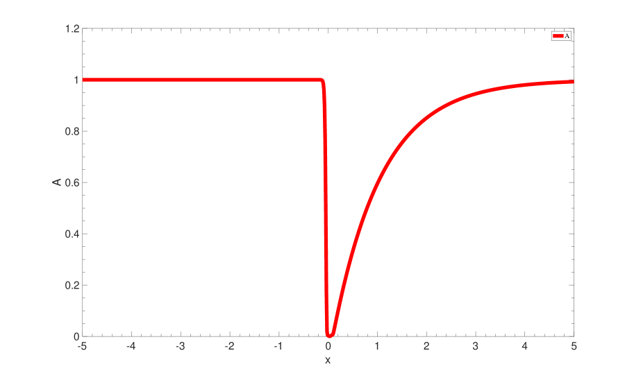
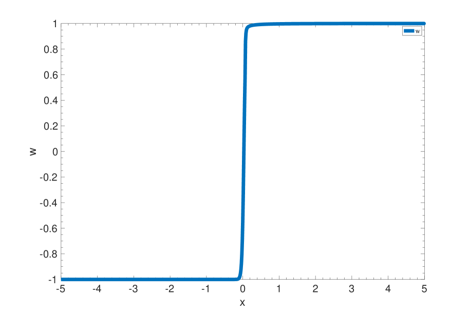
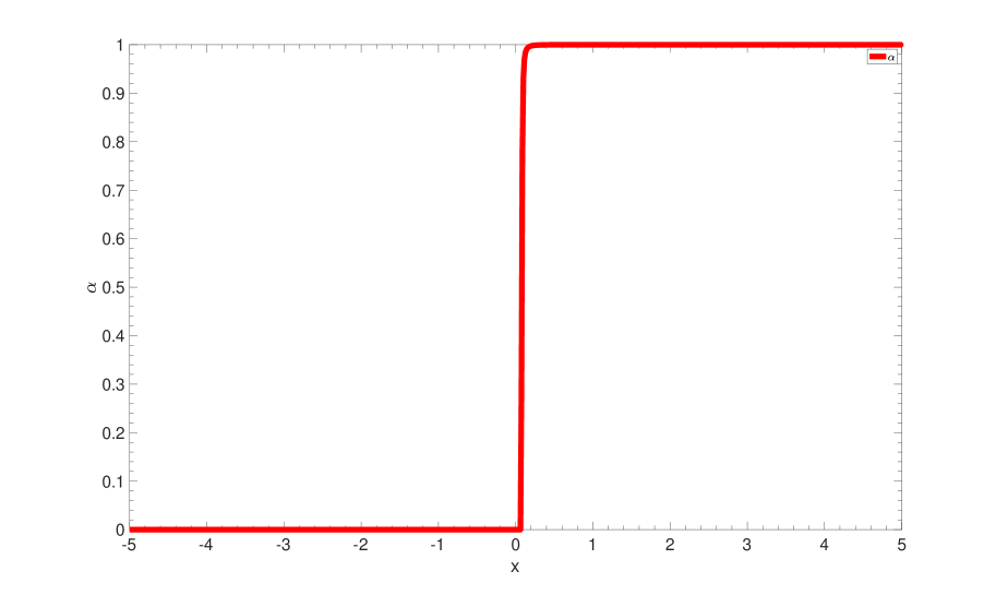
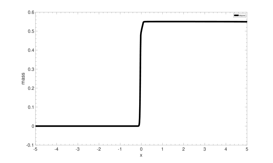
Figure 1: (a): The $A$ is regular $r=0$. There is no horizon and $\min(A)=0.0004$. Using different initial data, one can get different smooth steady state solution, such as $W(x,0)=\tanh(10(x-0.23))$, the $\min(A)=0.0026.$ (b): $W$ is smooth and approximates $1$ in the far field and close to -1 near $r=0.$ (c): $\alpha$ closes to 0 as $x\to-\infty$ ($r\to 0$). (d): The mass increases to the total mass $M=0.54.$

We consider the linear perturbation of EYM systems in this section. For convenience, we write the metric as

$$ds^{2}=-A\alpha^{2}dt^{2}+\frac{1}{A}dr^{2}+r^{2}(d\theta^{2}+\sin^{2}\theta d\phi^{2})$$

and denote the $SU(2)$ gauge potential by

$${\mathfrak{A}} =a_{0}\tau_{r}dt+a_{1}\tau_{r}dr+(1+W)(\tau_{\theta}\sin\theta d\phi-\tau_{\phi}d\theta)$$

$$\ \ \ \ \ +u(\tau_{\theta}d\theta+\tau_{\phi}\sin\theta d\phi),$$

where $A,\alpha,a_{0},a_{1},W,u$ are functions of $r,t$ and

$$\tau_{r} =\tau_{1}\sin\theta\cos\phi+\tau_{2}\sin\theta\sin\phi+\tau_{3}\cos\theta,$$ (14)

$$\tau_{\theta} =\tau_{1}\cos\theta\cos\phi+\tau_{2}\cos\theta\sin\phi-\tau_{3}\sin\theta,$$ (15)

$$\tau_{\phi} =-\tau_{1}\sin\phi+\tau_{2}\cos\phi$$ (16)

with $\tau_{i},i=1,2,3$ are the usual Pauli spin matrices. For more details, see Ref. Ge3 . In the static case, we set $a_{0}=a_{1}=u=0.$ We will consider the spherically symmstric perturbations for our regular solution obtained above. In history, many people study the instability of Bantnik-McKinnon solutions and colored black holes solutions. The unstable mode found bu Zhou-Straumannun2 belong to perturbations within the original Bantnik-McKinnon ansatz. Beside these even-parity modes there is a second class of exponentially growing modesGe1 ; Ge2 , which was called ”sphaleron-like” instability. The complete set of perturbation can be decoupled into two groups: even sector (“gravitational”) and odd sector (“sphaleron”), because the parity transformation $\theta\to\pi-\theta,\phi\to\phi+\pi$ is a symmetry operation Ge1 ; Ge2 .

The even-parity sector perturbation ansatz are

$$W(t,r) =W_{0}+\varepsilon\tilde{W}(r)e^{i\sigma t},$$ (17)

$$A(t,r) =A_{0}+\varepsilon\tilde{A}(r)e^{i\sigma t},$$ (18)

$$\alpha(t,r) =\alpha_{0}+\varepsilon\tilde{\alpha}(r)e^{i\sigma t},$$ (19)

where $W_{0},A_{0},\alpha_{0}$ are the background solution obtained above (See Fig. 1).

We obtain the following ODE eigenvalue problem

$$-\sigma^{2}\tilde{W}=A_{0}^{2}\alpha_{0}^{2}\tilde{W}_{rr}+\alpha_{0}^{2}C_{3}\tilde{W}_{r}+\tilde{W}\alpha_{0}^{2}(C_{1}-\frac{4}{r}C_{2}A_{0}W_{0,r}),$$

where

$$C_{1} =A_{0}(\frac{1-3W_{0}^{2}}{r^{2}}-\frac{4W_{0}(W_{0}^{2}-1)}{r^{3}}W_{0,r}),$$

$$C_{2} =2A_{0}W_{0,rr}+\frac{1}{r^{2}}W_{0}(1-W_{0}^{2}),$$

$$C_{3} =\frac{A_{0}}{r}(1-A_{0}-\frac{(1-W_{0}^{2})^{2}}{r^{2}}).$$

The first eigenvalue is given by

$$\sigma^{2}=24607.8079188817,$$

which show that the $\sigma\in\mathbb{R}$, and show the solution of the linear equation would not grow.

Next, we consider the odd-parity sector perturbation

$$a_{0}(t,r) =\varepsilon\tilde{a}_{0}(r)e^{i\sigma t},$$ (20)

$$a_{1}(t,r) =\varepsilon\tilde{a}_{1}(r)e^{i\sigma t},$$ (21)

$$u(t,r) =\varepsilon\tilde{u}(r)e^{i\sigma t}.$$ (22)

The odd-parity (“sphaleron”) perturbation equations are given by

$$\alpha_{0}^{2}A_{0}^{2}(-\tilde{u}_{rr}+W_{0}\tilde{a}_{1,r}-\frac{W_{0}^{2}-1}{A_{0}r^{2}}\tilde{u}) =\sigma^{2}\tilde{u},$$ (23)

$$\frac{2}{r^{2}}\alpha_{0}^{2}A_{0}(W_{0,r}\tilde{u}-W_{0}\tilde{u}_{r}+W_{0}^{2}\tilde{a}_{1}) =\sigma^{2}\tilde{a}_{1}.$$ (24)

The first eigenvalue of the above system is

$$\sigma^{2}=24359.6486332623.$$

Hence, the $\sigma\in\mathbb{R}$ and sphaleron sector will not grow.

III Acknowledgments

We would like to thank Professor George Lavrelashvili for valuable remarks and comments.

IV Appendix: Light cone and Curvature

Here, we will study the geometry structure of the smooth solution. First, we consider the null geodesic, which are given by

$$\frac{dt}{dr}=\pm\frac{1}{A\alpha}$$ (25)

or, in $x$ coordinate

$$t_{x}=\pm\frac{e^{x}}{A\alpha}.$$

We integral the null geodesic and show the light cones in Fig. 2.

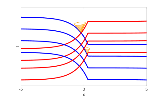
Figure 2: Light cones of the smooth solution.

The Ricci scalar curvature is computed in Fig. 3, and we found it is $0$ everywhere.

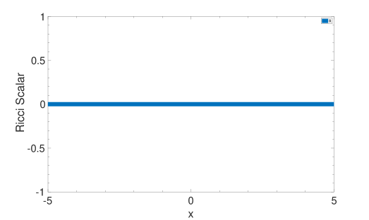
Figure 3: The Ricci scalar curvature is 0 everywhere.

References

- (1) R. Bartnik and J. McKinnon, Particle-like solutions of the Einstein Yang-Mills equations, Phys. Rev. Lett. 61, 141 (1988).
- (2) J. A. Smoller, A. G. Wasserman, S.-T. Yau, and J. B. McLeod, Smooth static solutions of the Einstein-Yang/Mills equation, Commun. Math. Phys. 143, 115-147 (1991).
- (3) J. A. Smoller, A. G. Wasserman, Existence of infinitely-many smooth, static, global solutions of the Einstein/Yang-Mills equations, Commun. Math. Phys. 151, 303-325 (1993).
- (4) J. A. Smoller and A. Wasserman, Regular solutions of the Einstein-Yang-Mills equations, J. Math. Phys. 36, 4301-4323 (1995).
- (5) N. Straumann and Z. H. Zhou, Instability of the Bartnik-mckinnon solution of the Einstein-Yang-Mills Equations, Phys. Lett. B 237, 353-356 (1990).
- (6) P. Bizon, Colored black holes, Phys. Rev. Lett. 64, 2844 (1990).
- (7) M. S. Volkov and D. V. Gal’tsov, NonAbelian Einstein-Yang-Mills black holes, Sov. J. Nucl. Phys. 51, 1171 (1990).
- (8) H. P. Künzle and A. K. M. Masood-ul-Alam, Spherically symmetric static Einstein-Yang-Mills fields, J. Math. Phys. 31, 928 (1990).
- (9) M. W. Choptuik, J. Chmaj, and P. Bizoń, Critical Behavior in Gravitational Collapse of a Yang-Mills Field, Phys. Rev. Lett. 773, 424-427 (1996).
- (10) M. Maliborski and O. Rinne, Critical phenomena in the general spherically symmetric Einstein-Yang-Mills system, Phys. Rev. D 97, 044053 (2018).
- (11) M. W. Choptuik, E. W. Hirschmann, and R. L. Marsa. New Critical Behavior in Einstein-Yang-Mills Collapse, Phys. Rev. D 60, 124011 (1999).
- (12) O. Rinne, Formation and decay of Einstein-Yang-Mills black holes, Phys. Rev. D 90, 124084 (2014).
- (13) J. A. Smoller, A. G. Wasserman, and S.-T. Yau, Existence of black-hole solutions for the Einstein-Yang/Mills equations, Commun. Math. Phys. 154, 377-401 (1993).
- (14) N. Straumann and Z. H. Zhou, Instability of a colored black hole solution, Phys. Lett. B 243, 33-35 (1990).
- (15) P. Bizon and R. M. Wald, The colored black hole is unstable, Phys. Lett. B 267, 173-174 (1991).
- (16) Z. H. Zhou and N. Straumann, Nonlinear perturbations of Einstein-Yang-Mills solitons and non-abelian black holes, Nucl. Phys. B 360, 180-196 (1991).
- (17) N. E. Mavromatos and E. Winstanley, Aspects of hairy black holes in spontaneously broken Einstein-Yang-Mills systems: Stability analysis and entropy considerations, Phys. Rev. D, 53, 3190 (1996).
- (18) G. Lavrelashvili and D. Maison, A remark on the instability of the Bartnik-McKinnon solutions, Phys. Lett. B, 343, 214-217 (1995).
- (19) M. S. Volkov, O. Brodbeck, G. Lavrelashvili, and N. Straumann, The number of sphaleron instabilities of the Bartnik-McKinnon solitons and non-Abelian black holes, Phys. Lett. B 349, 438-442 (1995).