Study of $SU(2)$ gauge theories with multiple Higgs fields in different representations

Abstract

We study two different SU(2) gauge-scalar theories in 3 and 4 spacetime dimensions. Firstly, we focus on the 3 dimensional SU(2) theory with multiple Higgs fields in the adjoint representation, that can be mapped to cuprate systems in condensed matter physics which host a rich phase diagram including high-Tc superconductivity. It has been proposed that the theory with 4 adjoint Higgs fields can be used to explain the physics of hole-doped cuprates for a wide range of parameters. We show exploratory results on the phase diagram of the theory.

On the other hand, we are interested in the 4 dimensional theory with 2 sets of fundamental scalar (Higgs) fields, which is relevant to the 2 Higgs Doublet Model (2HDM), a proposed extension to the Standard Model of particle physics. The goal is to understand the particle spectrum of the theory at zero temperature and the electroweak phase transition at finite temperature. We present exploratory results on scale setting and the multi-parameter phase diagram of this theory.

1 Introduction

Lattice gauge theories coupled to scalar (Higgs) fields have been studied for several decades, due to their applicability in diverse fields of physics. We study two $SU(2)$ gauge theories coupled to Higgs fields in different representations, one being relevant to BSM physics and the other to high-$T_{c}$ superconducting cuprate systems. The lattice action for $D$-dimensional $SU(2)$ gauge theory with $N_{h}$ Higgs fields transforming in a given representation of the gauge group can be written as

$$S=\beta\sum_{x}\sum_{\mu<\nu}^{D}\left(1-\frac{1}{2}\Tr U_{\mu\nu}(x)\right)-\sum_{x}\sum_{\mu=1}^{D}\sum_{n=1}^{N_{h}}\sum_{i,j=1}^{N_{g}}\kappa_{n}(\Phi_{n}^{i}(x))^{\ast}\tilde{U}_{\mu}^{ij}(x)\Phi_{n}^{j}(x+\hat{\mu})$$

$$+\sum_{x}\sum_{n=1}^{N_{h}}\sum_{i=1}^{N_{g}}(\Phi_{n}^{i}(x))^{\ast}\Phi_{n}^{i}(x)+\sum_{x}\sum_{n=1}^{N_{h}}\lambda_{n}\left(\sum_{i=1}^{N_{g}}(\Phi_{n}^{i}(x))^{\ast}\Phi_{n}^{i}(x)-1\right)^{2}+V(\{\Phi_{n}\})\,,$$ (1)

where the first term is the usual Wilson plaquette action of gauge links $U_{\mu}(x)$ in the fundamental representation and $\tilde{U}_{\mu}^{ij}(x)$ indicates the $SU(2)$ gauge link in a given representation, with the indices $i,j=1,\ldots,N_{g}$, $N_{g}$ being the dimension of the said representation. The dimensionless Higgs fields $\Phi_{n}^{i}(x)$ are real/complex-valued depending on the representation, with $n=1\ldots N_{h}$ being the flavor index and $i=1\ldots N_{g}$ being the representation index. Depending on the global symmetries of the theory, there can be other quartic interaction terms for the Higgs fields which are denoted by $V(\{\Phi_{n}\})$.

2 Gauge theory for cuprates on the lattice

Since their discovery in the 1980s, cuprate superconductors have been a topic of tremendous interest in the condensed matter community. Along with high temperature superconductivity (at $\sim$ 150 $K$), these materials exhibit rich phases with the variation of temperature, doping densities, magnetic field, etc. Of special interest are hole-doped cuprates near optimal doping, where there exist a plethora of unconventional phases with charge density wave (CDW) and/or nematic order that are unveiled from beneath the superconducting phase at strong magnetic field [1]. It is imperative to understand the microscopic mechanism behind these phases to explain the superconducting phenomenon.

In Ref. [2], the authors proposed a $SU(2)$ gauge theory with $N_{h}=4$ Higgs fields transforming under the adjoint representation of the gauge group in ($2+1$) spacetime dimensions to explain the $2d$ hole-doped cuprate systems around optimal doping. The usual confining phase of the gauge theory corresponds to the Fermi liquid phase at high doping density while the broken (Higgs) phase can be mapped to the unconventional phases at underdoping including the pseudogap phase. In contrast to the $N_{h}=1$ case [3], the $SU(2)$ gauge symmetry is expected to be broken into either $U(1)$-symmetric or $Z(2)$-symmetric Higgs phases.

The continuum action of the theory is given in Ref. [2]. We aim to study the phase diagram by discretising the continuum action on a $3d$ Euclidean spacetime lattice. In Eq. 1, we set $D=3$, $N_{h}=4$ and the couplings $\kappa_{n}=\kappa$ and $\lambda_{n}=\lambda$ for this theory. The $3\times 3$ adjoint representation link variable matrix can be written in terms of the $2\times 2$ fundamental link variable as $\tilde{U}_{\mu}^{ij}(x)=2\Tr(T^{i}U_{\mu}(x)T^{j}U_{\mu}^{\dagger}(x))$, where $T^{i}=\sigma_{i}/2$ are the generators of $SU(2)$ in the fundamental representation, $\sigma_{i}$ being the Pauli matrices. For convenience, we separate the complex Higgs fields $\mathcal{H}_{x/y}$ defined in [2] as $\boldsymbol{\mathcal{H}}_{x}=\varphi_{1}+i\varphi_{2}$, $\boldsymbol{\mathcal{H}}_{y}=\varphi_{3}+i\varphi_{4}$, to four real 3-component adjoint Higgs fields $\varphi_{n}^{i}(x)$ ($n=1,\ldots,4$ and $i=1,2,3$). The dimensionless Higgs fields for the lattice action (cf. Eq. 1) is related to the dimensionful $\varphi_{n}^{i}(x)$ as $\Phi_{n}^{i}=\sqrt{a/\kappa}\varphi_{n}^{i}$ , with $a$ being the lattice spacing. Since there are only local terms in the Higgs potential, we suppress the spacetime index and write the potential as

$$V(\{\Phi_{n}\})=4\lambda\sum_{x} \sum_{n\neq m}^{4}V_{mm}V_{nn}+\hat{u_{1}}\sum_{x}\sum_{m,n}^{4}g_{mn}V_{mm}V_{nn}+4\hat{u_{3}}\sum_{x}\sum_{n\neq m}^{4}V_{mn}V_{mn}$$

$$+\hat{u_{2}}\sum_{x} \left[\sum_{n=1}^{4}(V_{nn})^{2}+4(V_{12})^{2}+4(V_{34})^{2}-2V_{11}V_{22}-2V_{33}V_{44}\right]\,,$$ (2)

where we have used the abbreviation $V_{mn}=\Tr(\Phi_{m}\Phi_{n})$ and the Higgs fields have been expressed as $\Phi_{n}=\Phi_{n}^{i}T^{i}$ such that $2\Tr(\Phi_{m}\Phi_{n})=\sum_{i=1}^{3}\Phi_{m}^{i}\Phi_{n}^{i}$. In the 2^nd term, the $g_{mn}$ are symmetric and given by $g_{mm}=g_{12}=g_{34}=1$ and -1 for all other combinations. The dimensionful continuum couplings in Eq. (2.1c) of Ref. [2] are related to the dimensionless lattice couplings as follows

$$\beta=\frac{4}{g^{2}a},\quad\lambda=u_{0}a\kappa^{2},\quad s=\frac{1}{a^{2}}\left[\frac{1}{\kappa}-3-\frac{2\lambda}{\kappa}\right],\quad\hat{u_{i}}=u_{i}a\kappa^{2}\quad(i=1,2,3).$$ (3)

The terms in the Higgs potential are constrained by the global symmetries of the hole-doped cuprate systems. The breaking of these symmetries leads to different phases within the Higgs phase. These Higgs phases, labelled by (A)-(G) in Fig. 1, can be characterised by various gauge-invariant bilinear combinations combinations of the adjoint Higgs fields (cf. [2]),

$$\phi=\Phi_{1}^{i}\Phi_{1}^{i}+\Phi_{2}^{i}\Phi_{2}^{i}-\Phi_{3}^{i}\Phi_{3}^{i}-\Phi_{4}^{i}\Phi_{4}^{i}\quad \text{(Ising nematic order)},$$

$$\Phi_{x}=\Phi_{1}^{i}\Phi_{1}^{i}-\Phi_{2}^{i}\Phi_{2}^{i}+2i\Phi_{1}^{i}\Phi_{2}^{i}\quad (\text{CDW order at wave vector }K_{x}),$$

$$\Phi_{y}=\Phi_{3}^{i}\Phi_{3}^{i}-\Phi_{4}^{i}\Phi_{4}^{i}+2i\Phi_{3}^{i}\Phi_{4}^{i}\quad (\text{CDW order at wave vector }K_{y}),$$

$$\Phi_{+}=\Phi_{1}^{i}\Phi_{3}^{i}-\Phi_{2}^{i}\Phi_{4}^{i}+i(\Phi_{1}^{i}\Phi_{4}^{i}+\Phi_{2}^{i}\Phi_{3}^{i})\quad (\text{CDW order at wave vector }K_{x}+K_{y}),$$

$$\Phi_{-}=\Phi_{1}^{i}\Phi_{3}^{i}+\Phi_{2}^{i}\Phi_{4}^{i}+i(\Phi_{1}^{i}\Phi_{4}^{i}-\Phi_{2}^{i}\Phi_{3}^{i})\quad (\text{CDW order at wave vector }K_{x}-K_{y}),$$ (4)

where the sum over the adjoint index $i$ is implied. The different broken phases in the Higgs phase have been predicted through mean-field analysis [2] and is shown in Fig. 1. In the analysis, the coupling $s$ is chosen negative enough to be in the broken phase and the quartic coupling $u_{0}$ is chosen large enough to stabilise the potential. A follow-up work [4] studied the model numerically in the strong gauge coupling limit with the global $O(N_{h}=4)$-invariant action obtained by setting the couplings $u_{1}=u_{2}=u_{3}$. In this approximation, the existence of the confinement phase and broken phases, symmetric under $U(1)$ and $Z(2)$, were confirmed. Another recent study [5] in the $O(4)$ limit also demonstrated the existence of the two differently-broken Higs phases. In this work, we study the complete action, proposed in [2], non-perturbatively for the first time.

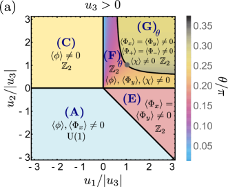
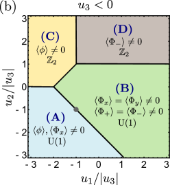
Figure 1: Mean-field prediction of the various broken phases in the 3d $SU(2)$ gauge theory with $N_{h}=4$ adjoint Higgs, taken from Ref. [2]. The expectation values of the observables for the different phases depicted above correspond to a particular choice in which the adjoint Higgs fields get the vev and there are other symmetry-equivalent choices. In general, the observables $\Phi_{x,y}$ and $\Phi_{+,-}$ can be complex and hence, we consider the modulus of them in our study. Moreover, the phases with non-zero $\expectationvalue{\Phi_{x}}$ ($\expectationvalue{\Phi_{+}}$) can also have a non-zero $\expectationvalue{\Phi_{y}}$ ($\expectationvalue{\Phi_{-}}$) for other choices of the vev. In plot (b), the expectation values of $\Phi_{x,y}$ and $\Phi_{+,-}$ in phase (B) are all equal.

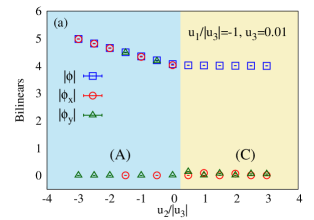
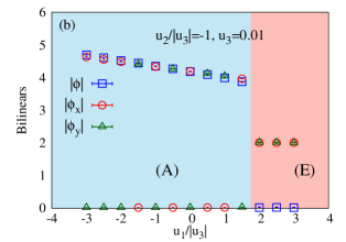
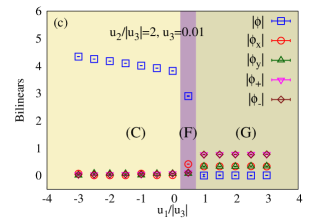
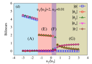
Figure 2: Expectation values of bilinears across the phase diagram for $u_{3}>0$. The results have been obtained from simulations on $12^{3}$ lattices.

2.1 Simulation details

We perform Monte Carlo simulations of the gauge theory with adjoint Higgs fields. We have used Hybrid Monte Carlo (HMC) algorithm for generating configurations of the gauge and Higgs fields and have measured the expectation values of various bilinears in Eq. 4. Our preliminary results include measurements on $8^{3}$ and $12^{3}$ lattices. The gauge coupling is set to $\beta=8.0$ for all simulations. In order to be in the stable broken phase, the lattice couplings $\kappa$ and $\lambda$ (related to the continuum couplings $s$ and $u_{0}$ by Eq. 3) are chosen to be $3.0$ and $1.0$ respectively. To study the predicted phase diagrams in Fig. 1, we set the lattice quartic coupling $\hat{u_{3}}$ to be $0.09$ and $-0.09$, and vary $\hat{u}_{1,2}$ such that the ratios $\hat{u_{1}}/|\hat{u_{3}}|$ and $\hat{u_{2}}/|\hat{u_{3}}|$ are in the range $[-3.5:3.5]$.

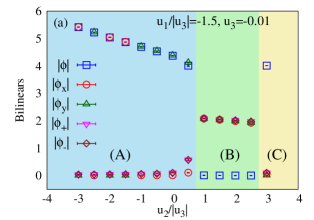
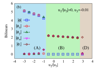
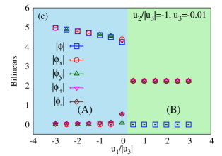
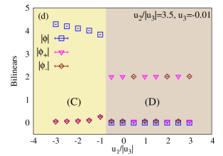
Figure 3: Results for expectation values of bilinears across the phase diagram for $u_{3}<0$ obtained from simulations on $12^{3}$ lattices.

2.2 Results

Our preliminary lattice simulations of the theory appear to qualitatively support the mean-field phase diagram. We have performed horizontal and vertical scans of the positive/negative $u_{3}$ phase diagram in Fig. 1. We plot the variation of the expectation values of the bilinears as a function of $u_{1}/|u_{3}|$ ($u_{2}/|u_{3}|$) at fixed $u_{2}/|u_{3}|$ ($u_{1}/|u_{3}|$).

For $u_{3}>0$, Fig. 2 shows the scanning results. In Fig. 2 (a), the variation of the bilinears $|\phi|$, $|\Phi_{x}|$ and $|\Phi_{y}|$ is shown as a function of $u_{2}/|u_{3}|$ where the value of $u_{1}/|u_{3}|$ is fixed at -1. In agreement with the mean-field scenario in Fig 1 (a), we find a transition between phases (A) and (C) around $u_{2}/|u_{3}|=0$. The bilinear $|\phi|$ is non-zero in both the phases while $|\Phi_{x}|$ or $|\Phi_{y}|$, either of which is non-zero in (A) vanishes sharply at the transition to phase (C). Next, Fig. 2 (b) depicts the transition between phases (A) and (E) as a function of $u_{1}/|u_{3}|$ at a fixed $u_{2}/|u_{3}|=-1$. The bilinear $|\phi|$ is non-zero in phase (A) and goes to zero in (E), while the bilinears $|\Phi_{x}|$ and $|\Phi_{y}|$ are equal and non-zero in phase (E). Fig. 2 (c) cuts across the phase diagram (in Fig. 1 (a)) horizontally and shows the transitions between phases (C) and (F) followed quickly by the transition to (G) from (F). Along with $|\phi|$, $|\Phi_{x}|$ and $|\Phi_{y}|$, we plot the bilinears $|\Phi_{+}|$ and $|\Phi_{-}|$ which are zero in phases (A), (C) and (E). In the transition between phases (F) and (G), the bilinear $|\phi|$ goes from non-zero in (F) to zero in (G) while $|\Phi_{x}|$ and $|\Phi_{y}|$ show similar behavior as in the transition from phase (A) to (E). The bilinears $|\Phi_{+}|$ and $|\Phi_{-}|$ become equal and non-zero in phase (G). Finally, in Fig. 2 (d), the variation of the bilinears along the vertical direction of the phase diagram (cf. Fig. 1 (a)) at a fixed $u_{1}/|u_{3}|=2$, shows the transitions from phase (A)-(E), (E)-(F) and (F)-(G).

Next we discuss our results for the case of $u_{3}<0$ corresponding to the mean-field phase diagram in Fig. 1 (b). The variation of the bilinears as a function of $u_{2}/|u_{3}|$ at a fixed $u_{1}/|u_{3}|=-1.5$ is shown in Fig. 3 (a). It depicts the transition from phase (A)-(B) and then from phase (B)-(C). The bilinear $|\phi|$ vanishes in phase (B) while $|\Phi_{x}|$, $|\Phi_{y}|$, $|\Phi_{+}|$ and $|\Phi_{-}|$ become non-zero and equal.The behavior of the observables in phases (A) and (C) are same as in the case of $u_{3}>0$ discussed earlier. Along the same direction, Fig. 3 (b) displays the transitions from phase (A)-(B) and phase (B)-(D) at a fixed value of $u_{1}/|u_{3}|=0$. All the bilinears vanish in phase (D) except for $|\Phi_{+}|$ or $|\Phi_{-}|$. Next in Fig. 3 (c), the bilinears exhibit a transition from phase (A) to (B) as a function of $u_{1}/|u_{3}|$ at fixed $u_{2}/|u_{3}|=-1$. Lastly, the transition from phase (C) to (D) is seen by varying the bilinears $|\phi|$, $|\Phi_{+}|$ and $|\Phi_{-}|$ with respect to $u_{1}/|u_{3}|$ at $u_{2}/|u_{3}|=3.5$.

3 Two Higgs Doublet Model on the lattice

3.1 Background and Action

The scalar field structure of the Standard Model (SM) is the simplest way to realize electroweak symmetry breaking. It consists of a single SU(2) Higgs doublet in the fundamental representation. On the other hand, the fermion structure of the theory includes various families, with mixing involved. One of the simplest extensions of the SM is the addition of extra Higgs fields in the fundamental representation. In this work we consider the Two Higgs Doublet Model (2HDM). The introduction of a second Higgs doublet is motivated by the existence of multiple families of fermions in the SM. It contains appealing features for model building, such as new sources of CP violation and a first-order electroweak phase transition (EWPT) that drives baryogenesis [6, 7]. However, since no deviation from the SM has been observed at the LHC, it is crucial that one of the two Higgs doublets in 2HDM mimics that of the SM. This is known as the “alignment” requirement. In supersymmetry-inspired 2HDM, it was shown that the masses of the scalar particles in the second Higgs doublet are around 5 TeV [8]. This places the extra Higgs doublet in the decoupling limit, leading to the fact that it cannot be discovered in direct searches at the LHC.

It has been suggested that the alignment requirement can be fulfilled without decoupling [9, 10, 11, 12]. In this scenario, the masses of the extra scalar particles are typically at around or below 1 TeV. Such a realisation of alignment is facilitated with choices of coupling and mixing strengths in 2HDM. Notably, as pointed out in Ref. [12], it may require certain couplings amongst the scalar fields to be strong. Combining this with the trivality property of these couplings, it is necessary to investigate the viability of this scenario by examining carefully the relationship amongst the spectrum, the cut-off scale, and the couplings. To study the above alignment phenomenon without decoupling, as well as the nature of EWPT, it is necessary to employ non-perturbative methods to survey the model. For this purpose, lattice field theory is the most reliable tool, and is what we pursue in this work.

In the lattice action in Eq. 1, we set $D=4$ and $N_{h}=2$. In this case, the complex Higgs doublet on the lattice $\Phi_{n}(x)=(\varphi_{n}^{2}(x)+i\varphi_{n}^{1}(x),\varphi_{n}^{0}(x)-i\varphi_{n}^{3}(x))$ ($n=1,2$) is related to the dimensionful continuum field $\phi_{n}(x)$ as $\Phi_{n}(x)=a/\sqrt{\kappa}\phi_{n}(x)$. For convenience, we combine the four degrees of freedom of the complex doublet in the quaternion representation as a matrix, $\hat{\Phi}_{n}(x)=\frac{1}{\sqrt{2}}\sum_{\alpha=0}^{3}\theta_{\alpha}\varphi^{\alpha}_{n}(x)$ where $\theta_{0}=1_{2\times 2}$, $\theta_{i}=\sigma_{i}$. The gauge-Higgs interaction term in Eq. 1 now contains the fundamental $SU(2)$ gauge link $U_{\mu}(x)$ and is written compactly as $-2\kappa_{n}\Tr\left(\hat{\Phi}_{n}^{\dagger}(x)U_{\mu}(x)\hat{\Phi}_{n}(x+\hat{\mu})\right)$. With the quartic couplings taken to be real, the local Higgs potential takes the form

$$V(\{\hat{\Phi}_{n}(x)\}) =2\mu^{2}\Tr\left(\hat{\Phi}_{1}^{\dagger}(x)\hat{\Phi}_{2}(x)\right)+\xi_{1}\Tr\left(\hat{\Phi}_{1}^{\dagger}(x)\hat{\Phi}_{1}(x)\right)\Tr\left(\hat{\Phi}_{2}^{\dagger}(x)\hat{\Phi}_{2}(x)\right)+\xi_{2}\Tr\left(\hat{\Phi}_{1}^{\dagger}(x)\hat{\Phi}_{2}(x)\right)^{2}$$

$$+2\Tr\left(\hat{\Phi}_{1}^{\dagger}(x)\hat{\Phi}_{2}(x)\right)\left[\xi_{3}\Tr\left(\hat{\Phi}_{1}^{\dagger}(x)\hat{\Phi}_{1}(x)\right)+\xi_{4}\Tr\left(\hat{\Phi}_{2}^{\dagger}(x)\hat{\Phi}_{2}(x)\right)\right].$$ (5)

It should be noted that the quartic couplings $\lambda_{i}$ in Eq. 1 are denoted by $\eta_{i}$ below.

3.2 Observables and Gradient Flow

To analyse the phase structure of the system we looked at observables which can signal a phase transition, although not being exactly order parameters. The squared Higgs length, $\expectationvalue{\rho_{n}^{2}}=1/V\expectationvalue{\sum_{x}\rho_{n}(x)^{2}}$ with $\rho_{n}^{2}=\det\hat{\Phi}_{n}(x)$ for each Higgs doublet was considered. It is non-zero in both the phases but increases rapidly in the Higgs phase. Along with the average plaquette $P=\frac{1}{12V}\sum_{\square}\Tr{U_{\square}}$, the following gauge-invariant links were also considered,

$$L_{\hat{\Phi}_{n}}=\frac{1}{8V}\sum_{x,\mu}\Tr{\hat{\Phi}_{n}^{\dagger}(x)U_{\mu}(x)\hat{\Phi}_{n}(x+\hat{\mu})}\,,\quad L_{\alpha_{n}}=\frac{1}{8V}\sum_{x,\mu}\Tr{\alpha_{n}^{\dagger}(x)U_{\mu}(x)\alpha_{n}(x+\hat{\mu})}\,,$$ (6)

where $\alpha_{n}$ is the “angular” part of the quaternion Higgs field, $\hat{\Phi}_{n}=\rho_{n}\alpha_{n}$. The quantity $L_{\alpha}$ is particularly useful since it is bounded between -1 and 1 and can be used to compare the strength of the transition at different parameter regions [13].

Additionally, since it important to know the scale of the theory, gradient flow observables were used. The gauge invariant action density, $\expectationvalue{E(x,t)}=-1/2\expectationvalue{\Tr G_{\mu\nu}(x,t)G_{\mu\nu}(x,t)}$, with $G_{\mu\nu}$ being the flowed gauge field strength ($t$ is the flow time), has been studied. Two discretizations, namely the plaquette and the clover, for the gauge field strength are considered. The idea of this scale setting is that the fields are flowed until the action density reaches a specific value $\mathcal{E}_{0}$ – this has an associated flow time value $t=t_{0}$, and thus a scale $\mu=1/\sqrt{8t_{0}}$ at which this happens. By doing this we can determine the relative scales for computations performed at different bare couplings.

In our theory, we are interested in the Higgs phase of the theory and, we want the renormalized gauge coupling at the $W$ boson mass to be $g^{2}\equiv 4\pi\alpha_{W}\simeq 0.5$ [14]. Using the relation between the renormalized coupling and the flowed action density [15], we will obtain the physical theory by requiring

$$\mathcal{E}_{0}\equiv t^{2}\expectationvalue{E(t)}\Big{|}_{t=t_{0}}=\frac{9g^{2}}{128\pi^{2}}(1+\mathcal{O}(g^{2}))\simeq 0.0036\Big{|}_{\mu=1/\sqrt{8t_{0}}=m_{W}},$$ (7)

and the SM Higgs mass being equal to its physical value.

3.3 Simulation details

The simulations have been performed using HMC algorithm on GPU machines [16] . This allows the use of large lattices. The results from the HMC code was independently verified using a Metropolis algorithm code. In our current simulations, the phase transition from the confinement to the Higgs phase was studied as a function of $\kappa_{1}=\kappa_{2}$ at different $\beta$ values. For all runs, the couplings $\mu^{2}=0.2$, $\eta_{1}=\eta_{2}=0.5$ and $\xi_{i}=0.1$ $(i=1,\ldots,4)$ have been kept fixed.

3.4 Results

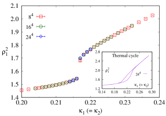
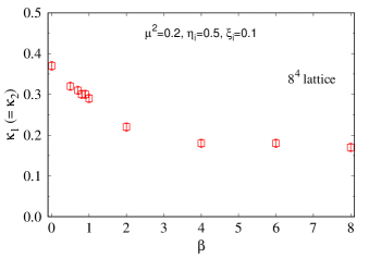
Figure 4: Left: Preliminary result of the variation of the Higgs length $\rho_{1}^{2}$ with respect to $\kappa_{1}$ ($=\kappa_{2}$) at $\beta=2.0$ on $8^{4}$, $16^{4}$ and $24^{4}$ lattices. Inset: Thermal cycle of $\rho_{1}^{2}$ obtained on a $24^{4}$ lattice displaying a hysteresis behavior. Right: Preliminary results of the phase transition points in the $\beta$ - $\kappa_{1}$ ($=\kappa_{2}$) plane found on $8^{4}$ lattices. Results in both plots have been obtained at fixed $\mu^{2}=0.2,\eta_{i}=0.5$ and $\xi_{i}=0.1$.

A preliminary analysis of the phase transition, obtained by changing the $\kappa_{1}=\kappa_{2}$ values at a constant $\beta$, allowed us to identify the Higgs/confinement phases in the space of bare parameters. To evaluate the phase transition line in the $\beta$ - $\kappa_{1}$/$\kappa_{2}$ plane, we calculate the gauge invariant observables on $8^{4}$, $16^{4}$ and $24^{4}$ lattices. We show a preliminary result of the hopping parameter $\kappa_{1}$ $(=\kappa_{2})$ dependence the Higgs length $\expectationvalue{\rho_{1}^{2}}$ at $\beta=2.0$ on different lattices in the left plot in Fig. 4. The observable shows a jump indicative of a first-order phase transition around $\kappa_{1}=\kappa_{2}=0.217$ at this parameter set. In the inset, we show results from a thermal cycle run which clearly indicates a hysteresis loop. The thermal cycle has been obtained by taking the system through steps of $\kappa_{1}=\kappa_{2}=0.01$ with only 5 HMC trajectories at each point, starting from $\kappa_{1}=\kappa_{2}=0.14$ to $0.29$ and coming back. The system was allowed to equilibrate at the end points. At each point in the up or down paths of the cycle, the HMC run uses the last configuration from the previous point as the initial start. Further analysis via finite size scaling or observation of a two-state signal near the transition needs to be obtained to confirm the position and order of the transition. We show the transition points obtained at different values in the $(\beta,\kappa_{1}=\kappa_{2})$ phase diagram in the right plot of Fig. 4. The transition at intermediate $\beta$ show a strong jump in the observables (as seen in Fig. 4 left) but become gradually continuous at smaller or larger $\beta$. These results are similar to the case of SU(2) gauge theory with a single Higgs doublet [13].

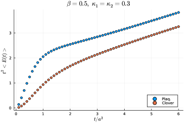
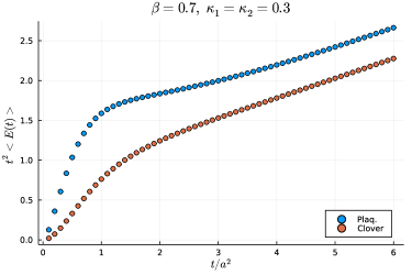
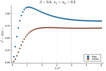
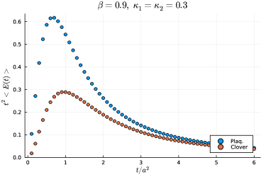
Figure 5: $t^{2}\expectationvalue{E(t)}$ for $\kappa_{1}=\kappa_{2}=0.3$ and various $\beta$ values from 500 flow measurements. For all the runs, the quadratic coupling is $\mu^{2}=0.2$ and the quartic couplings are $\eta_{i}=0.5$ and $\xi_{i}=0.1$.

As for scale setting, our preliminary investigations of the flow of the plaquette and clover action density, $t^{2}\expectationvalue{E(t)}$, as a function of the flow time, $t/a^{2}$, are shown in Fig. 5. The quantity $t^{2}\expectationvalue{E(t)}$ is proportional to the gauge coupling in the gradient-flow scheme [see Eq. (7)]. Results presented in this figure indicate a significant change in behaviour of the gauge coupling with flow time as one increases the $\beta$ at a fixed $\kappa_{1}=\kappa_{2}$. At smaller $\beta=0.5,0.7$, the system is in the confining phase and it goes over to the Higgs phase as $\beta$ is increased, (see Fig. 4). Plots in the top row of Fig. 5 exhibit $t^{2}\expectationvalue{E(t)}$ as a function of $t$ in the confining phase, In this phase, behaviour similar to that of QCD is observed, although the lattice artefacts are sizeable in simulations with these two $\beta$ values. The bottom-row plots in Fig. 5 demonstrate the same quantity in the Higgs phase. It is noticed that at long distance, the gauge coupling in the gradient-flow scheme decreases with the renormalisation scale. Qualitative understanding of this behaviour can be achieved by studying the one-loop $\beta{-}$ function of the gauge coupling in the SU(N) gauge theory coupled to $n_{s}$ scalar fields,

$$\beta_{{\mathrm{SU(N)-scalar}}}=\mu\frac{dg}{d\mu}=-\frac{b_{0}g^{3}}{16\pi^{2}}+{\mathcal{O}}(g^{5})\,,\,\,{\mathrm{where}}\,\,b_{0}=\frac{11N-n_{s}}{3}\,.$$ (8)

Below the $M_{W}$ threshold in the Higgs phase, the gauge bosons are integrated out, and $N=0$ in $b_{0}$, resulting in a positive $\beta_{{\mathrm{SU(N)-scalar}}}$. The short-distance ($t/a^{2}\rightarrow 0$) behaviour shown in these plots seems to be consistent with the presence of asymptotic freedom. Although this can also be understood by having $N=2$ in Eq. (8) (above the $M_{W}$ threshold), lattice artefacts are very significant in this regime, where further detailed investigation is needed in the future.

4 Conclusions and outlook

We study the $3d$ $SU(2)$ gauge theory with four flavors of Higgs fields transforming under the adjoint representation. The theory was proposed to describe the physics of hole-doped cuprate systems near optimal doping in Ref. [2]. In our lattice study, we have qualitatively confirmed the mean-field predictions of the theory in the Higgs phase. We show the existence of the various broken phases signalled by the expectation values of gauge-invariant order parameters bilinear in the Higgs fields. We are currently working on identifying the order of the phase transitions and finding out a purported deconfined quantum critical point, as predicted in [2].

In the lattice 2HDM, we calculate gauge invariant observables to investigate phase transition lines in the $(\beta,\kappa_{1}=\kappa_{2})$ phase diagram. This is the first-time study of complete potential with real couplings. Our preliminary results indicate the existence of first-order transition separating the confinement and Higgs phases of the theory. However, this needs to be established. We implement the gradient flow for the $SU(2)$ gauge fields in the 2HDM for setting the scale. Our goal is to study the mass spectrum of the two Higgs doublet model with the physical $W$ boson and Higgs boson masses.

5 Acknowledgements

The work of AH is supported by the Taiwanese MoST grant 110-2811-M-A49-501-MY2 and 111-2639-M-002-004-ASP. The work of CJDL is supported by the Taiwanese MoST grant 109-2112-M-009-006-MY3 and 111-2639-M-002-004-ASP. AR and GT acknowledge support from the Generalitat Valenciana (genT program CIDEGENT/2019/040) and the Ministerio de Ciencia e Innovacion PID2020-113644GB-I00. The work of MS is supported by the Taiwanese MoST grant NSTC 110-2811-M-002-582-MY2, NSTC 108-2112-M-002-020-MY3 and 111-2124-M-002-013-. The authors gratefully acknowledge the computer resources at Artemisa, funded by the European Union ERDF and Comunitat Valenciana as well as the technical support provided by the Instituto de Física Corpuscular, IFIC (CSIC-UV), and the computer resources at AS, NTHU, NTU, NYCU and DESY, Zeuthen.

References

- [1] C. Proust and L. Taillefer, Annual Review Of Condensed Matter Physics. 10, 409-429 (2019)
- [2] S. Sachdev, H. D. Scammell, M. S. Scheurer and G. Tarnopolsky, Phys. Rev. B 99 (2019) no.5, 054516.
- [3] A. Hart, O. Philipsen, J. D. Stack and M. Teper, Phys. Lett. B 396 (1997), 217-224.
- [4] H. D. Scammell, K. Patekar, M. S. Scheurer and S. Sachdev, Phys. Rev. B 101 (2020) no.20, 205124.
- [5] C. Bonati, A. Franchi, A. Pelissetto and E. Vicari, Phys. Rev. B 104 (2021) no.11, 115166.
- [6] M. Trodden, [arXiv:hep-ph/9805252 [hep-ph]].
- [7] L. Fromme, S. J. Huber and M. Seniuch, JHEP 11 (2006), 038.
- [8] P. Athron et al. [GAMBIT], Eur. Phys. J. C 77 (2017) no.12, 879.
- [9] J. F. Gunion and H. E. Haber, Phys. Rev. D 67 (2003), 075019.
- [10] M. Carena, I. Low, N. R. Shah and C. E. M. Wagner, JHEP 04 (2014), 015.
- [11] P. S. Bhupal Dev and A. Pilaftsis, JHEP 12 (2014), 024 [erratum: JHEP 11 (2015), 147].
- [12] W. S. Hou and M. Kikuchi, EPL 123 (2018) no.1, 11001.
- [13] M. Wurtz, R. Lewis and T. G. Steele, Phys. Rev. D 79 (2009), 074501.
- [14] W. Langguth, I. Montvay and P. Weisz, Nucl. Phys. B 277 (1986), 11-49.
- [15] M. Lüscher, JHEP 08 (2010), 071 [erratum: JHEP 03 (2014), 092].
- [16] Ramos, A., https://igit.ific.uv.es/alramos/latticegpu.jl/