Modelling Large Dimensional Datasets with Markov Switching Factor Models

Abstract

We study a novel large dimensional approximate factor model with regime changes in the loadings driven by a latent first order Markov process. By exploiting the equivalent linear representation of the model, we first recover the latent factors by means of Principal Component Analysis. We then cast the model in state-space form, and we estimate loadings and transition probabilities through an EM algorithm based on a modified version of the Baum-Lindgren-Hamilton-Kim filter and smoother that makes use of the factors previously estimated. Our approach is appealing as it provides closed form expressions for all estimators. More importantly, it does not require knowledge of the true number of factors. We derive the theoretical properties of the proposed estimation procedure, and we show their good finite sample performance through a comprehensive set of Monte Carlo experiments. The empirical usefulness of our approach is illustrated through an application to a large portfolio of stocks.

Keywords: Large Factor Model, Markov Switching, Baum-Lindgren-Hamilton-Kim Filter and Smoother, Principal Component Analysis, Stock Returns.

JEL Codes: C34, C38, C55, G10.

1 Introduction

This paper develops a comprehensive approach for the analysis of large dimensional models exhibiting an approximate factor structure, in which the loadings are subject to regime shifts driven by a first order latent Markov process. We label these large dimensional Markov Switching factor models.

Since the works of Hamilton (1989), and Diebold and Rudebusch (1996), and inspired by the seminal paper of Goldfeld and Quandt (1973), Markov switching models have been widely used in the empirical analysis of macroeconomic and financial time series data: Hamilton (2016) gives an overview from a macroeconomic perspective, and Doz et al. (2020) present recent evidence of their usefulness for turning-point detection and macroeconomic forecasting; Guidolin (2011), and Ang and Timmermann (2012), provide a comprehensive survey in relation to financial markets; see also Qu and Zhuo (2021) and references therein for more recent advances. However, to the very best of our knowledge, the existing literature has focused on small dimensional Markov switching models, which are not applicable to high dimensional cross-sections. We aim at filling a gap in the literature by studying Markov switching models as applied to large panels.

There now exists strong empirical evidence that macroecononomic and financial variables exhibit an approximate factor structure, as stressed in Giannone et al. (2021). This nature of the data naturally leads to approximate latent factor specifications as a tool to model time series comovement in large dimensional cross-sections. For example, following the seminal contribution of Chamberlain and Rothschild (1983), static approximate factor representations have been considered in Connor and Korajczyk (1986) to develop measures of portfolio performance, and in Stock and Watson (2002a, b) to forecast large macroeconomic panels and to build indexes of macroeconomic activity. The full inferential theory is developed by Bai (2003). Settings allowing for dynamic factor representations have been also extensively studied: see Forni et al. (2017) and references therein. A broad overview of large factor models is provided in Stock and Watson (2016). To the very best of our knowledge, the vast majority of existing contributions has looked at the linear setting. However, this may not be flexible enough to accommodate the discrete regimes typically observed in macroeconomic and financial series.

A number of contributions have extended linear static factor models to allow for discrete shifts in the loadings by assuming that these shifts are driven by an observable state variable. A first and growing stream of literature assumes that this state variable is a deterministic time index, which leads to a factor model with structural instability in the loadings: see Breitung and Eickmeier (2011), Corradi and Swanson (2014), Baltagi et al. (2016), Cheng et al. (2016), Barigozzi et al. (2018), Barigozzi and Trapani (2020), Duan et al. (2023), among others, and Bai and Han (2016) for a survey of the literature. The presence of structural breaks implies that regime changes are not recurrent and are related to events such as technological changes or shifts in monetary policy regimes. Alternatively, the states could be driven by the realisation of an observable stationary variable with respect to a reference value, in which case a threshold factor model would arise: see Massacci (2017, 2023). Under this set up, regimes are recurrent and associated to cyclical events such as business and financial cycles. Smoothly varying loadings are considered in Motta et al. (2011) and Pelger and Xiong (2022). Finally, Chen et al. (2023) follow Su and Wang (2017) and propose a time-varying matrix factor model with smooth changes in the loadings driven by a time index.

In this paper, we are interested in large dimensional factor models in relation to recurrent regime changes. A major drawback of threshold factor models is that they require a priori identification of the state variable. This may lead to model misspecification and unreliable empirical findings should the wrong state variable be employed to identify the regimes. In order to overcome this problem, we resort to the two-state Markov switching model of Goldfeld and Quandt (1973) with a latent state variable, and we extend it to allow for an underlying large dimensional factor structure. Within this setting, we make the following major methodological contributions: we propose an algorithm to estimate the conditional state probabilities, as well as the loadings and the factors; and we derive the asymptotic properties of the estimators for loadings and factors. Remarkably, our results do not require knowledge of the true number of factors in any regime, and they are robust to the number of factors being unknown and estimated. This is an important aspect of our paper. Estimating the number of factors is challenging in a linear setting, as evidenced by the high number of relevant contributions: Bai and Ng (2002), Alessi et al. (2010) and Ahn and Horenstein (2013), develop model selection criteria; Kapetanios (2010), Onatski (2010), and Trapani (2018), propose inferential procedures. Dealing with an unknown number of factors clearly becomes even more engaging in the presence of regimes driven by a latent state variable and it therefore is an important contribution of our paper.

To the very best of our knowledge, the literature on large dimensional Markov Switching factor models is still in its infancy. However, two existing contributions are important to discuss. First, Liu and Chen (2016) study a model similar to ours, but their definition of common factors differs from ours in that they consider factors that are pervasive along the time dimension rather than along the cross-sectional dimension. As a consequence, their idiosyncratic components are assumed to be white noise. Second, Urga and Wang (2022) study a set up similar to ours, with two important differences: they assume a priori knowledge of the number of factors; they consider a model with serially homoskedastic idiosyncratic components. In addition, the Maximum Likelihood estimation approach of Urga and Wang (2022) adapts the EM algorithm by Rubin and Thayer (1982) and Bai and Li (2012) to the case of Gaussian mixtures, where the weights are given by the probability of the latent variables to be in a given regime. Note that, to the very best of our knowledge, no existing contribution has formally proved that in the factor model case the EM algorithm is a contraction, namely that it converges to the Maximum Likelihood estimator. The approach in Urga and Wang (2022) leads to estimators for the unknown parameters that do not have closed form solutions. This in an additional important difference with respect to our approach, which instead leads to closed form solutions.

Our approach is as follows. We introduce an algorithm to estimate factors, loadings, and transition probabilities, which extends to high dimensional factor models the state-space approach advanced in Hamilton (1989) and Kim (1994) to handle low dimensional Markov switching autoregressive models. In particular, we generalize the the Baum-Lindgren-Hamilton-Kim filter and smoother, the original version of which was proposed to estimate Markov-switching VAR models: for example, see the reviews by Guidolin (2011), Krolzig (2013), Hamilton (2016), and Guidolin and Pedio (2018). An important feature of our approach is that it provides closed form expressions for all estimators. Even more remarkably, we not require a priori knowledge of the number of factors in each regime, which is instead needed by Urga and Wang (2022).

We obtain our theoretical results by exploiting the well known property that a factor model with neglected discrete regime changes admits an equivalent representation with a higher number of factors: for example, see the discussions in Breitung and Eickmeier (2011), Barigozzi et al. (2018), and Duan et al. (2023), in the case of structural breaks; and Massacci (2023) for threshold factor models. We use this property to estimate the latent factors by means of Principal Component Analysis (PCA) as applied to the linear representation. We then input these estimated factors into our algorithm, which allows us to recover the loadings and the transition probabilities. We then derive the asymptotic properties of the estimator for the loadings: we prove the asymptotic normality; we characterise the bias, which is induced both by the well known identification problem, and by the incomplete information related to the underlying data generated process. We also study the asymptotic properties of the estimated factors, which are obtained by projecting the data onto the estimated loadings. We corroborate our theoretical results through a comprehensive set of Monte Carlo experiments, which confirm the good finite sample properties of the estimation procedure we propose.

Finally, we assess the empirical validity of our model through an application to a large set of U.S. stock returns. Markov switching models have been widely used to capture the cyclical behaviour of small-dimensional portfolios of financial assets: see Guidolin (2011), and Ang and Timmermann (2012), and references therein. We contribute to this literature by applying the Markov switching factor model to a large dimensional portfolio of financial assets. Our results show that the regimes described by the model closely follow U.S. business cycle dynamics. In addition, an inspection of the estimated loadings allows us to identify level and slope factors. Therefore, our model could be employed to explain cross-sectional differences in average returns, and to then run conditional asset pricing tests when the regimes are driven by a latent first order Markov process. This would complement the findings in Massacci et al. (2021), who identify the regimes based on the return from the underlying stock market.

The rest of the paper is organised as follows. Section 2 introduces the two-state model. Section 3 describes the estimation algorithm. Section 4 derives the asymptotic theory. Section 5 presents two further results related to estimation of the number of factors and to underspecification of the number of regimes. Section 6 briefly discusses the issue of unobserved heterogeneity. Section 7 runs a comprehensive set of Monte Carlo experiments. Section 8 applies our model to a large number of industry equity portfolios. Finally, Section 9 concludes. Details about the estimation algorithm are given in Appendix A. Mathematical derivations are collected in Appendices B and C.

Notation

We denote as $\otimes$ the Kronecker product, with $\odot$ the Hadamard (element-wise) product, and with $\oslash$ the element-wise ratio. For a vector $\bm{v}=(v_{1}\cdots v_{m})^{\prime}$ we denote its Euclidean norm as $\|\bm{v}\|=\sqrt{\sum_{i=1}^{m}v_{i}^{2}}$. For a matrix $\mathbf{C}$ we denote the spectral norm as $\|\mathbf{C}\|=\sqrt{\mu_{1}(\mathbf{C}\mathbf{C}^{\prime})}$, where $\mu_{1}(\mathbf{C}\mathbf{C}^{\prime})$ indicates the largest eigenvalue of $\mathbf{C}\mathbf{C}^{\prime}$. If $\text{rk}(\mathbf{C})=r<\infty$, then, we sometimes use the same notation $\|\mathbf{C}\|$ to denote also the Frobenius norm $\|\mathbf{C}\|_{F}=\sqrt{\text{tr}(\mathbf{C}\mathbf{C}^{\prime})}$. Indeed, $\|\mathbf{C}\|_{F}\leq\sqrt{r}\|\mathbf{C}\|$ and since it is always true that $\|\mathbf{C}\|\leq\|\mathbf{C}\|_{F}$, then, bounding the Frobenius or the spectral norm is asymptotically equivalent.

For a scalar discrete random variable $Z$, the notation $\mathsf{P}(Z=z)$ is its probability mass function computed using the true value of the parameters. For random variables $\mathbf{Y}$ and $\mathbf{W}$ the notations $\mathsf{E}[\mathbf{Y}]$ and $\mathsf{E}[\mathbf{Y}|\mathbf{W}]$ are the expectation and conditional expectation given $\mathbf{W}$, respectively, computed with respect to the true distributions $F_{Y}(\mathbf{y})$ and $F_{Y|W}(\mathbf{y}|\mathbf{W})$ which in turn are computed using the true value of the parameters. If, in place of the true value of the parameters, we use an estimate of the parameters, say $\widehat{\theta}$, then we adopt the notations $\mathsf{P}_{\widehat{\theta}}(Z=z)$, $\mathsf{E}_{\widehat{\theta}}[\mathbf{Y}]$, and $\mathsf{E}_{\widehat{\theta}}[\mathbf{Y}|\mathbf{W}]$, respectively.

Finally, we let $\mathbf{I}_{m}$ be the identity matrix of dimension $m$, $\bm{\iota}_{m}$ an $m$-dimensional vector of ones, and $\mathbf{0}$ any matrix or vector of zeros whose dimensions depend on the context.

2 Markov switching factor model

2.1 Setup

We study a two-state large dimensional Markov switching factor model. Formally, we consider

$$\mathbf{x}_{t} =\bm{\Lambda}_{1}\mathbf{f}_{1t}\mathbb{I}(s_{t}=1)+\bm{\Lambda}_{2}\mathbf{f}_{2t}\mathbb{I}(s_{t}=2)+\mathbf{e}_{t},\qquad t\in\mathbb{Z},$$ (1)

$$\mathbf{e}_{t} =\bm{\Sigma}_{e1}^{1/2}\mathbb{I}(s_{t}=1)\bm{\nu}_{t}+\bm{\Sigma}_{e2}^{1/2}\mathbb{I}(s_{t}=2)\bm{\nu}_{t}.$$ (2)

We assume that the elements of the $N\times 1$ vector process of observable dependent variables $\{\mathbf{x}_{t}\}$ have zero mean, and we consider the more general case in which they are allowed to have mean different from zero in Section 6; $\{\mathbf{f}_{jt}\}$ is the $r_{j}\times 1$ vector process of latent factors such that $r_{j}$ is fixed and $r_{j}\ll N$, for $j=1,2$; $\bm{\Lambda}_{j}$ is the $N\times r_{j}$ matrix of factor loadings with rows equal to $\bm{\lambda}_{ji}^{\prime}$, for $i=1,\ldots,N$ and $j=1,2$; $\{\mathbf{e}_{t}\}$ is the $N\times 1$ vector process of idiosyncratic components with innovations $\bm{\nu}_{t}\sim\left(\mathbf{0},\mathbf{I}_{N}\right)$. Note that we allow the elements of $\{\mathbf{e}_{t}\}$ to be both serially and cross-sectionally weakly correlated, and we refer to Section 4 for the specific assumptions. It is also important to point out that the number of factors $r_{j}$ within each state is allowed to be unknown.

The model in (1) and (2) explicitly allows for two regimes: the case in which the number of states is actually underspecified is dealt with in Section 5.2. Also, the number of factors $r_{1}$ and $r_{2}$ is allowed to change between the regimes: in this, our approach is more general than in Liu and Chen (2016), who assume that $r_{1}=r_{2}$ and the dimension of the factor space is a priori the same between the two regimes.

As it is standard in the literature, we assume that $s_{t}$ follows a discrete-state, homogeneous, irreducible and ergodic, first-order Markov chain such that

$$\begin{array}[]{lll}\mathsf{P}\left(s_{t+1}=j\left|s_{t}=i\right.\right)=p_{ij},&i,j=1,2,&\sum\limits_{j=1}^{2}p_{ij}=1,\end{array}$$

with matrix of transition probabilities

$$\mathbf{P}=\left(\begin{array}[]{cc}p_{11}&p_{12}\\ p_{21}&p_{22}\end{array}\right)=\left(\begin{array}[]{cc}p_{11}&1-p_{11}\\ 1-p_{22}&p_{22}\end{array}\right).$$ (3)

Defining the $2\times 1$ vector of state indicators

$$\bm{\xi}_{t}=\left[\begin{array}[]{c}\mathbb{I}(s_{t}=1)\\ \mathbb{I}(s_{t}=2)\end{array}\right],\qquad t\in\mathbb{Z},$$ (4)

allows us to write the transition equation

$$\bm{\xi}_{t}=\mathbf{P}^{\prime}\bm{\xi}_{t-1}+\mathbf{v}_{t},\qquad t\in\mathbb{Z},$$ (5)

where $\{\mathbf{v}_{t}\}$ is a discrete-valued zero mean martingale difference sequence whose elements sum to zero. Because, $\|\mathbf{P}\|<1$, $\{s_{t}\}$ follows an ergodic Markov chain, thus, there exists a stationary vector of probabilities $\bar{\bm{\xi}}$ satisfying:

$$\bar{\bm{\xi}}=\mathbf{P}^{\prime}\bar{\bm{\xi}}.$$

Hence, the elements of $\bar{\bm{\xi}}$ are long-run or unconditional state probabilities. In particular, we have $\bar{\bm{\xi}}=\mathsf{E}[\bm{\xi}_{t}]$, such that

$$\mathsf{E}[\bm{\xi}_{t}]=\mathsf{E}\left[\begin{array}[]{c}\mathbb{I}(s_{t}=1)\\ \mathbb{I}(s_{t}=2)\end{array}\right]=\left[\begin{array}[]{c}\mathsf{P}(s_{t}=1)\\ \mathsf{P}(s_{t}=2)\end{array}\right],$$ (10)

where $0<\mathsf{P}(s_{t}=j)<1$, for $j=1,2$, by Assumption 1 in Section 4 below, which makes the Markov chain irreducible. In particular, (3) and (10) are related by (see, e.g., Guidolin and Pedio, 2018, Chapter 9)

$$\mathsf{P}(s_{t}=1)=\frac{1-p_{22}}{2-p_{11}-p_{22}},\quad\mathsf{P}(s_{t}=2)=\frac{1-p_{11}}{2-p_{11}-p_{22}}.$$ (11)

Finally, unlike the low-dimensional model of Diebold and Rudebusch (1996), we do not specify the factor dynamics. In particular, Diebold and Rudebusch (1996) allow for regime-specific factor mean, whereas the loadings do not vary: in this setting, the variance of the dependent variables remains constant over time. On the other hand, the large-dimensional model in (1) and (2) allows for regime-specific covariance matrix of $\mathbf{x}$: this is relevant for modelling both macroeconomic variables and financial returns, as stressed in McConnell and Perez-Quiros (2000), and Perez-Quiros and Timmermann (2000, 2001), respectively. We will exploit this feature in the empirical analysis in Section 8, where we will use the model in (1) and (2) to model returns from a large equity portfolio.

2.2 State space representation

Let the $\left(r_{1}+r_{2}\right)\times 1$ vector process $\{\mathbf{g}_{t}\}$ be defined as

$$\mathbf{g}_{t}=\left[\begin{array}[]{c}\mathbf{f}_{1t}\\ \mathbf{0}\end{array}\right]\mathbb{I}(s_{t}=1)+\left[\begin{array}[]{c}\mathbf{0}\\ \mathbf{f}_{2t}\end{array}\right]\mathbb{I}(s_{t}=2)=\left[\begin{array}[]{c}\mathbf{f}_{1t}\\ \mathbf{f}_{2t}\end{array}\right]\odot\bm{\xi}_{t},\qquad t\in\mathbb{Z}.$$ (12)

Let $\mathbf{B}_{1}=[\bm{\Lambda}_{1}\ \mathbf{0}]$ and $\mathbf{B}_{2}=[\mathbf{0}\ \bm{\Lambda}_{2}]$, where $\mathbf{B}_{1}$ and $\mathbf{B}_{2}$ are $N\times\left(r_{1}+r_{2}\right)$ matrices. The model in (1), (2) and (5) admits the equivalent state space representation

$$\mathbf{x}_{t} =\left(\mathbf{B}_{1}\leavevmode\nobreak\ \mathbf{B}_{2}\right)\left(\bm{\xi}_{t}\otimes\mathbf{g}_{t}\right)+\left(\mathbf{\Sigma}_{e1}^{1\left/2\right.}\leavevmode\nobreak\ \mathbf{\Sigma}_{e2}^{1\left/2\right.}\right)\left(\bm{\xi}_{t}\otimes\mathbf{I}_{N}\right)\mathbf{e}_{t},\qquad t\in\mathbb{Z},$$ (13)

$$\bm{\xi}_{t} =\mathbf{P}^{\prime}\bm{\xi}_{t-1}+\mathbf{v}_{t}.$$

Under standard assumptions, the term $\left(\mathbf{B}_{1}\leavevmode\nobreak\ \mathbf{B}_{2}\right)\left(\bm{\xi}_{t}\otimes\mathbf{g}_{t}\right)$ is identifiable up to a relabelling of the states. This means that the indices of the states can be permuted without changing the law governing the process for $\mathbf{x}_{t}$: on this, see Section 3 in Leroux (1992). Also note that, even for given $\bm{\xi}_{t}$, identification of $\textbf{B}_{1}$ and $\textbf{B}_{2}$, and therefore of the elements of $\{\textbf{g}_{t}\}$, is in general possible only up to an invertible linear transformation (see Bai, 2003).

2.3 Linear representation

Model (13) is observationally equivalent to a model with one change point affecting the loadings of all units (Barigozzi et al., 2018). It can then be rewritten as the $r_{1}+r_{2}$ linear factor model

$$\mathbf{x}_{t}=\mathbf{A}\mathbf{g}_{t}+\mathbf{e}_{t},\qquad t\in\mathbb{Z},$$ (14)

where $\mathbf{A}=\left[\mathbf{\Lambda}_{1}\leavevmode\nobreak\ \mathbf{\Lambda}_{2}\right]$. Then $\mathbf{A}$ and $\mathbf{g}_{t}$ may be estimated by standard Principal Component Analysis (PCA) (Stock and Watson, 2002a, b; Bai, 2003). Since PCA gives, as $N,T\to\infty$, consistent estimators of the factors up to premultiplication by an invertible matrix (see Bai, 2003), for ease of exposition we first consider estimation of the model in (13) by treating $\mathbf{g}_{t}$ as known. We then briefly review the implementation of PCA and its effect on the estimation of the model in Section 3.3.

2.4 Log-likelihood

We follow Bai and Li (2016) and estimate only the diagonal elements of $\bm{\Sigma}_{e1}$ and $\bm{\Sigma}_{e2}$ in (2). The parameters of interest are then partitioned as

$$\bm{\varphi}=\left[\mathrm{vec}\left(\mathbf{B}_{1}\right)^{\prime},\mathrm{vec}\left(\mathbf{B}_{2}\right)^{\prime},\text{diag}\left(\mathbf{\Sigma}_{e1}\right)^{\prime},\text{diag}\left(\mathbf{\Sigma}_{e2}\right)^{\prime}\right]^{\prime},\quad\bm{\rho}=\mathrm{vec}\left(\mathbf{P}\right),$$

so that the vector of parameters of interest, denoted as $\mathbf{q}$, is defined as

$$\mathbf{q}=\left[\bm{\varphi}^{\prime},\bm{\rho}^{\prime}\right]^{\prime}.$$

Let $\mathbf{X}=\left(\mathbf{x}_{1}^{\prime},\ldots,\mathbf{x}_{T}^{\prime}\right)^{\prime}$, $\bm{\mathcal{G}}=\left(\mathbf{g}_{1}^{\prime},\ldots,\mathbf{g}_{T}^{\prime}\right)^{\prime}$, where $\mathbf{X}$ is an $NT\times 1$ vector, $\bm{\mathcal{G}}$ is an $(r_{1}+r_{2})T\times 1$ vector. These are $T$-dimensional realizations of the stochastic processes $\{\mathbf{x}_{t}\}$ and $\{\mathbf{g}_{t}\}$, respectively. Moreover, let $\bm{X}_{v}$ be the $\sigma$-algebra generated by the random variables $\{\mathbf{x}_{t}\}_{t=1}^{v}$, for $v=1,\ldots,T$; in a similar way, define $\bm{G}_{v}$ as the $\sigma$-algebra generated by the random variables $\{\mathbf{g}_{t}\}_{t=1}^{v}$, for $v=1,\ldots,T$. And for simplicity we write $\bm{X}\equiv\bm{X}_{T}$ and $\bm{G}\equiv\bm{G}_{T}$.

The likelihood function, denoted by $f\left(\mathbf{X};\mathbf{q}\right)$, can be decomposed as

$$f\left(\mathbf{X};\mathbf{q}\right)=\frac{f\left(\mathbf{X},\bm{\mathcal{G}};\mathbf{q}\right)}{f\left(\bm{\mathcal{G}}\left|\bm{X};\mathbf{q}\right.\right)}=\frac{f\left(\mathbf{X}\left|\bm{G};\mathbf{q}\right.\right)f\left(\bm{\mathcal{G}};\mathbf{q}\right)}{f\left(\bm{\mathcal{G}}\left|\bm{X};\mathbf{q}\right.\right)}=\frac{f\left(\mathbf{X}\left|\bm{G};\mathbf{q}\right.\right)f\left(\bm{\mathcal{G}}\right)}{f\left(\bm{\mathcal{G}}\left|\bm{X};\mathbf{q}\right.\right)}:$$ (15)

in the last step we account for the fact that $f\left(\bm{\mathcal{G}};\mathbf{q}\right)\equiv f\left(\bm{\mathcal{G}}\right)$, since it does not depend on the parameters of our model, as we do not specify any dynamic model for the process $\{\mathbf{g}_{t}\}$.

Furthermore, following Krolzig (2013, Section 6.2), we have

$$f\left(\mathbf{X}\left|\bm{G};\mathbf{q}\right.\right)=f\left(\mathbf{X}\left|\bm{G};\bm{\varphi},\bm{\rho}\right.\right)=\sum_{\{\bm{\xi}_{t}\}_{t=1}^{T}\in\{0,1\}^{T}}f\left(\mathbf{X}\left|\bm{G},\{\bm{\xi}_{t}\}_{t=1}^{T};\bm{\varphi}\right.\right)\mathsf{P}\left(\{\bm{\xi}_{t}\}_{t=1}^{T}|\bm{G},\bm{\rho}\right).$$ (16)

Here, to avoid heavier notation, we use the same notation $\{\bm{\xi}_{t}\}_{t=1}^{T}$ both for a generic $T$ dimensional realization of the process $\{\bm{\xi}_{t}\}$ and for the $\sigma$-algebra generated by the random variables $\{\bm{\xi}_{t}\}_{t=1}^{T}$. Notice that the sum is over $2^{T}$ possible values since, given a realization for $\{\xi_{1t}\}_{t=1}^{T}$, the realizations of $\{\xi_{2t}\}_{t=1}^{T}$ are given by $\xi_{2t}=1-\xi_{1t}$ for all $t$.

Following the approach by Doz et al. (2012), and Barigozzi and Luciani (2019), and the one by Bai and Li (2016), all developed for QML estimation of linear factor models, for $f\left(\mathbf{X}\left|\bm{G},\{\bm{\xi}_{t}\}_{t=1}^{T};\bm{\varphi}\right.\right)$ we consider a misspecified Gaussian quasi-likelihood of an exact factor model. This implies that the idiosyncratic components are treated as if they were cross-sectionally uncorrelated. In addition, we also neglect serial correlation in the idiosyncratic components, thus treating them as if they were weak white noise processes. This approach is similar to the one also followed in Urga and Wang (2022). It is important to stress that we are not assuming that the idiosyncratic components are uncorrelated, as we are just considering likelihood estimation of a misspecified model. In the linear case, Bai and Li (2016), and Barigozzi and Luciani (2019), show that such misspecification is asymptotically negligible as $N,T\to\infty$. Under this setup, and using the Markov property of $\{\bm{\xi}_{t}\}$, up to omitted constant terms we have

$$\log f \left(\mathbf{X}\left|\bm{G},\{\bm{\xi}_{t}\}_{t=1}^{T};\bm{\varphi}\right.\right)=\sum_{t=1}^{T}\log f\left(\mathbf{x}_{t}\left|\mathbf{g}_{t},\bm{\xi}_{t};\bm{\varphi}\right.\right)$$ (17)

$$\simeq-\dfrac{1}{2}\sum\limits_{t=1}^{T}\log\det\mathbf{\Sigma}_{et}-\frac{1}{2}\sum_{t=1}^{T}\left\{\mathbf{x}_{t}-\left(\mathbf{B}_{1}\leavevmode\nobreak\ \mathbf{B}_{2}\right)\left(\bm{\xi}_{t}\otimes{\mathbf{g}}_{t}\right)\right\}^{\prime}\left(\mathbf{\Sigma}_{et}\right)^{-1}\left\{\mathbf{x}_{t}-\left(\mathbf{B}_{1}\leavevmode\nobreak\ \mathbf{B}_{2}\right)\left(\bm{\xi}_{t}\otimes{\mathbf{g}}_{t}\right)\right\},$$

where $\mathbf{\Sigma}_{et}=\left(\text{diag}(\mathbf{\Sigma}_{e1})\leavevmode\nobreak\ \text{diag}(\mathbf{\Sigma}_{e2})\right)\left(\bm{\xi}_{t}\otimes\mathbf{I}_{N}\right)$. Note that in this case the likelihood (16) is not Gaussian; rather, it is a mixture of Gaussian distributions. Finally, again by the Markov property of $\{\bm{\xi}_{t}\}$, we can write

$$\mathsf{P}\left(\{\bm{\xi}_{t}\}_{t=1}^{T}|\bm{G};\bm{\rho}\right) =\prod_{t=1}^{T}\mathsf{P}\left(\bm{\xi}_{t}|\bm{\xi}_{t-1},\bm{G};\bm{\rho}\right)\mathsf{P}\left(\bm{\xi}_{0}\right).$$ (18)

3 Estimation

In this section, we assume that the data generating process is characterised by two regimes as in the model in (1) and (2). In Section 5.2 we study the case in which the model is underspecified and the data generating process exhibits a higher number of regimes. We also assume that the dimension of the vector $\mathbf{g}_{t}$ in (14) is known. Should this not be the case, the dimension of $\mathbf{g}_{t}$ can be determined using information criteria such as those proposed in Bai and Ng (2002), Alessi et al. (2010) and Ahn and Horenstein (2013), or inferential techniques such as those developed in Onatski (2010), and Trapani (2018). This issue is discussed also in Section 5.1. For example, in the empirical analysis in Section 8, we use the criteria developed in Ahn and Horenstein (2013).

In what follows, Section 3.1 defines the steps of the proposed Expectation Maximization (EM) algorithm. Section 3.2 describes the Baum-Lindgren-Hamilton-Kim filter and smoother. Section 3.3 details the estimator for the factor space. Section 3.4 discusses the estimator for the parameters. Section 3.5 deals with initialization and convergence of the algorithm.

3.1 EM algorithm

The algorithm outlined in this section is a generalization of the procedure proposed by Krolzig (2013, Chapter 5). The EM algorithm is made of two steps repeated at each iteration $k\geq 0$. The E step involves taking the expected value of the log-likelihood derived from (15) conditional on $\bm{X}$ given an estimate of the parameters $\widehat{\mathbf{q}}^{\left(k\right)}$, namely

$$\log f\left(\mathbf{X};\mathbf{q}\right)=\mathsf{E}_{\mathbf{\widehat{q}}^{\left(k\right)}}\left[\log f\left(\mathbf{X}\left|\bm{G};\mathbf{q}\right.\right)\left|\bm{X}\right.\right]+\mathsf{E}_{\mathbf{\widehat{q}}^{\left(k\right)}}\left[\log f\left(\bm{\mathcal{G}}\right)\left|\bm{X}\right.\right]-\mathsf{E}_{\mathbf{\widehat{q}}^{\left(k\right)}}\left[\log f\left(\bm{\mathcal{G}}\left|\bm{X};\mathbf{q}\right.\right)\left|\bm{X}\right.\right].$$

The M step solves the constrained maximization problem with respect to $\mathbf{q}=\left[\bm{\varphi}^{\prime},\bm{\rho}^{\prime}\right]^{\prime}$, that is

$$\left({\widehat{\bm{\varphi}}}^{\left(k+1\right)},{\widehat{\bm{\rho}}}^{\left(k+1\right)}\right) =\arg\max_{\bm{\varphi},\bm{\rho}}\mathsf{E}_{\mathbf{\widehat{q}}^{\left(k\right)}}\left[\log f\left(\mathbf{X}\left|\bm{G};\bm{\varphi},\bm{\rho}\right.\right)\left|\bm{X}\right.\right]$$

$$\text{s.t.}\quad\mathbf{P}\bm{\iota}_{2}=\bm{\iota}_{2},$$ (19)

where the constraints ensure that probabilities add up to one. In principle, in the M step we should also account for the term $\mathsf{E}_{\mathbf{\widehat{q}}^{\left(k\right)}}\left[\log f\left(\bm{\mathcal{G}}\right)\left|\bm{X}\right.\right]$, which however in our context does not depend on any parameter.

It is well known that the iteration of these steps produces a series of increasing log-likelihoods. Indeed, $\mathsf{E}_{\mathbf{\widehat{q}}^{\left(k\right)}}\left[\log f\left(\bm{\mathcal{G}}\left|\bm{X};\mathbf{q}\right.\right)\left|\bm{X}\right.\right]$ does not contribute to the convergence of the EM algorithm (see Dempster et al., 1977, and Wu, 1983). Moreover, if the maximum is identified and unique, then the EM algorithm will eventually lead to the Maximum Likelihood estimator of $\mathbf{q}$. As shown below, the solution of the M step can be computed using the expressions given in (17) and (18). This solution is unique and in closed form. Therefore, no identification issue arises due to multiple maxima, or related to the existence of such maxima.

3.2 Baum-Lindgren-Hamilton-Kim filter and smoother

From (17) and (18), in order to compute the expected likelihood in the E step we need to compute $\mathsf{E}_{\widehat{\mathbf{q}}^{(k)}}[\bm{\xi}_{t}|\bm{X}]$, $\mathsf{E}_{\widehat{\mathbf{q}}^{(k)}}[\bm{\xi}_{t}\otimes\mathbf{g}_{t}|\bm{X}]$, and $\mathsf{E}_{\widehat{\mathbf{q}}^{(k)}}[(\bm{\xi}_{t}\otimes\mathbf{g}_{t})(\bm{\xi}_{t}\otimes\mathbf{g}_{t})^{\prime}|\bm{X}]=\mathsf{E}_{\widehat{\mathbf{q}}^{(k)}}[(\mathbf{I}_{2}\otimes\mathbf{g}_{t}\mathbf{g}_{t}^{\prime})|\bm{X}]$.

We start by considering the case in which both $\{\mathbf{g}_{t}\}_{t=1}^{T}$ is observed and the true value of the parameters $\mathbf{q}$ is known, while we postpone the discussion of the estimation of the factors to Section 3.3. Then, for the E step we just need to compute $\mathsf{E}[\bm{\xi}_{t}|\bm{X}]$, since in this case $\bm{\xi}_{t}$ and $\mathbf{g}_{t}$ are independent for all $t$. This is accomplished by means of a generalization the Baum-Lindgren-Hamilton-Kim filter and smoother explained in detail in Appendix A.1. It is an iterative procedure through which we first compute the sequences of conditional one-step-ahead predicted probabilities $\{\bm{\xi}_{t\left|t-1\right.}\}_{t=1}^{T}$, such that $\bm{\xi}_{t\left|t-1\right.}=\mathsf{E}\left[\bm{\xi}_{t}\left|\bm{X}_{t-1}\right.\right]$, and filtered probabilities $\{\bm{\xi}_{t\left|t\right.}\}_{t=1}^{T}$ such that $\bm{\xi}_{t|t}=\mathsf{E}[\bm{\xi}_{t}|\bm{X}_{t}]$. Second, by means of those sequences, we compute the sequence of smoothed probabilities $\{\bm{\xi}_{t\left|T\right.}\}_{t=1}^{T}$ such that $\bm{\xi}_{t|T}=\mathsf{E}[\bm{\xi}_{t}|\bm{X}]$.

The final recursions for the filtered probabilities are given by (e.g., see Krolzig, 2013, Chapter 5.1, and Hamilton, 1989)

$$\bm{\xi}_{t\left|t-1\right.} =\mathbf{P}^{\prime}\bm{\xi}_{t-1\left|t-1\right.},\quad t=1,\ldots,T,$$

$$\bm{\xi}_{t\left|t\right.} =\dfrac{\bm{\eta}_{t}\odot\bm{\xi}_{t\left|t-1\right.}}{\bm{\iota}_{2}^{\prime}\left(\bm{\eta}_{t}\odot\bm{\xi}_{t\left|t-1\right.}\right)},\quad t=1,\ldots,T,$$ (20)

where

$$\bm{\eta}_{t} =\left[\begin{array}[]{c}f\left(\mathbf{x}_{t}\left|\bm{\xi}_{t}=\left[1\leavevmode\nobreak\ 0\right]^{\prime},\mathbf{{g}}_{t}\right.\right)\\ f\left(\mathbf{x}_{t}\left|\bm{\xi}_{t}=\left[0\leavevmode\nobreak\ 1\right]^{\prime},\mathbf{{g}}_{t}\right.\right)\end{array}\right].$$ (23)

The filter can be started by setting either $\bm{\xi}_{0|0}=\left[1\leavevmode\nobreak\ 0\right]^{\prime}$, or, equivalently, $\bm{\xi}_{0|0}=\left[0\leavevmode\nobreak\ 1\right]^{\prime}$.

The final recursions for the smoothed probabilities are given by (e.g., see Krolzig, 2013, Chapter 5.2, and Kim, 1994)

$$\bm{\xi}_{t\left|T\right.}=\left[\mathbf{P}\left(\bm{\xi}_{t+1\left|T\right.}\oslash\bm{\xi}_{t+1\left|t\right.}\right)\right]\odot\bm{\xi}_{t\left|t\right.},\quad t=1,\ldots,T.$$ (24)

This backward recursion is initiated at $\bm{\xi}_{T|T}$, which is the last iteration of the filter in (20).

The above description of the Baum-Lindgren-Hamilton-Kim filter and smoother assumes that $\mathbf{q}$ and $\mathbf{g}_{t}$ are observed. However, in practice both need to be estimated. This is discussed in the next two Sections 3.3 and 3.4 below.

3.3 Estimating the factor space

In order to estimate the factors $\mathbf{g}_{t}$, and their dimension $r_{1}+r_{2}$, we exploit the fact that the Markov switching factor model in (1) is observationally equivalent to a linear factor model with $r_{1}+r_{2}$ common factors $\mathbf{g}_{t}$ and factor loadings $\mathbf{A}$: see Section 2.3 and, in particular, equation (14). The number of factors in (14) can be estimated using methods already available in the literature: for example, see Bai and Ng (2002), Onatski (2010), Ahn and Horenstein (2013), and Trapani (2018). The factors $\mathbf{g}_{t}$ can be estimated by PCA as follows. First, the estimator $\widehat{\mathbf{A}}$ of the loadings matrix $\mathbf{A}$ is obtained as $\sqrt{N}$ times the normalized eigenvectors corresponding to the $r_{1}+r_{2}$ largest eigenvalues of the sample $N\times N$ covariance matrix $T^{-1}\sum_{t=1}^{T}\mathbf{x}_{t}\mathbf{x}_{t}^{\prime}$. Second, the factors are estimated by linear projection of the data $\mathbf{x}_{t}$ onto the estimated loadings:

$$\widehat{\mathbf{g}}_{t}=\left(\widehat{\mathbf{A}}^{\prime}\widehat{\mathbf{A}}\right)^{-1}\widehat{\mathbf{A}}^{\prime}\mathbf{x}_{t}=\frac{1}{N}\widehat{\mathbf{A}}^{\prime}\mathbf{x}_{t},\quad t=1,\ldots,T.$$ (25)

This is the same approach followed by Stock and Watson (2002a). It is also the dual approach of the one adopted by Bai (2003). Consistency of $\widehat{\mathbf{A}}$ and $\widehat{\mathbf{g}}_{t}$ follow from Lemma 1 and Lemma 5(a) in Appendix B, respectively. Note that the steps described in this section do not require knowing the latent state indicator $\bm{\xi}_{t}$, and they can be carried out independently. Because of these results, $\bm{\xi}_{t}$ and $\widehat{\mathbf{g}}_{t}$ can also be treated as independent for all $t$. As a consequence, the Baum-Lindgren-Hamilton-Kim filter described in Section 3.2 can be implemented by just replacing the true factors $\mathbf{g}_{t}$ with their estimator $\widehat{\mathbf{g}}_{t}$ defined in (25).

3.4 Estimating the parameters

At each iteration $k\geq 0$ of the EM algorithm, the filtered and smoothed probabilities, given in (20) and (24), respectively, and the smoothed cross-probabilities given in (A.16), are computed using an estimator $\widehat{\mathbf{q}}^{(k)}$ of the parameters and an estimator $\widehat{\mathbf{g}}_{t}$ of the factors. Hereafter, we denote as $\bm{\xi}_{t|t}^{(k)}$, $\bm{\xi}_{t|T}^{(k)}$, and $\bm{\xi}_{t,t-1|T}^{(k)}$ such estimators. This defines the E step.

In the M step we have to solve the constrained maximization problem in (19). Here we just give the final results, while we refer to Appendix A.2 for their derivation. The estimates of the loadings $\mathbf{B}_{j}$, $j=1,2$, are given by

$$\mathbf{\widehat{B}}_{j}^{(k+1)}=\left(\sum_{t=1}^{T}{\xi}_{j,t\left|T\right.}^{(k)}\mathbf{x}_{t}\mathbf{\widehat{g}}_{t}^{\prime}\right)\left(\sum_{t=1}^{T}{\xi}_{j,t\left|T\right.}^{(k)}\widehat{\mathbf{g}}_{t}\mathbf{\widehat{g}}_{t}^{\prime}\right)^{-1},\quad j=1,2,$$ (26)

and, consistently with the fact that we use a mis-specified likelihood with uncorrelated idiosyncratic components, we set

$$[\widehat{\mathbf{\Sigma}}_{ej}^{(k+1)}]_{ii} =\left(\dfrac{\sum_{t=1}^{T}\left({x}_{it}-\mathbf{\widehat{b}}_{ji}^{(k+1)\prime}\mathbf{\widehat{g}}_{t}\right)^{2}}{\sum_{t=1}^{T}{\xi}_{j,t\left|T\right.}^{(k)}}\right),\quad i=1,\ldots,N,\quad j=1,2,$$ (27)

$$[\widehat{\mathbf{\Sigma}}_{ej}^{(k+1)}]_{ik} =0,\quad i,k=1,\ldots,N,\quad i\neq k,\quad j=1,2,$$

where $\mathbf{\widehat{b}}_{ji}^{(k+1)\prime}$ is the $i$th row of $\mathbf{\widehat{B}}_{j}^{(k+1)}$. Concerning the estimates of $\bm{\rho}$ which are subject to the adding up condition,

$$\widehat{\bm{\rho}}^{(k+1)}=\left[\sum_{t=1}^{T}\bm{\xi}_{t,t-1|T}^{(k)}\right]\oslash\left[\bm{\iota}_{2}\otimes\sum_{t=0}^{T-1}\bm{\xi}_{t|T}^{(k)}\right].$$ (28)

By letting $k^{*}$ be the last iteration of the EM algorithm, we define our final estimator of the parameters as $\widehat{\mathbf{q}}\equiv\widehat{\mathbf{q}}^{(k^{*}+1)}$, as given by (26), (27), and (28). The final estimator of $\bm{\xi}_{t}$ is defined as $\widehat{\bm{\xi}}_{t|T}\equiv\bm{\xi}_{t|T}^{(k^{*}+1)}$, i.e., obtained by running one last time the Baum-Lindgren-Hamilton-Kim filter using the final estimates of the parameters.

3.5 Initialization and convergence of the EM algorithm

To start the algorithm we need initial estimators $\widehat{\mathbf{q}}^{(0)}$ for the parameters. Specifically, we set $\widehat{\mathbf{B}}_{1}^{(0)}=\widehat{\mathbf{B}}_{2}^{(0)}=\widehat{\mathbf{A}}$, as defined in Section 3.3. Then, given also $\widehat{\mathbf{g}}_{t}$ as in (25), let $\widehat{\mathbf{e}}_{t}=\mathbf{x}_{t}-\widehat{\mathbf{A}}\widehat{\mathbf{g}}_{t}$, and we set $\widehat{\bm{\Sigma}}_{e1}^{(0)}=\widehat{\bm{\Sigma}}_{e2}^{(0)}=\text{diag}\left(T^{-1}\sum_{t=1}^{T}\widehat{\mathbf{e}}_{t}\widehat{\mathbf{e}}_{t}^{\prime}\right)$. Finally, we set

$$\widehat{\mathbf{P}}^{(0)}=\left(\begin{array}[]{cc}0.5+\omega_{1}&1-0.5-\omega_{1}\\ 1-0.5-\omega_{2}&0.5+\omega_{2}\end{array}\right),$$

where $\omega_{1},\omega_{2}\in(0,0.5)$ and $\omega_{1}>\omega_{2}$. This initialization implicitly identifies state 1 as the most probable one, i.e., it is the state with largest unconditional probability as defined in (11).

We say that the EM algorithm converged at iterations $k^{*}$, where $k^{*}$ is the first value of $k$ such that:

$$\frac{\left|\log f\left(\mathbf{X}\left|\bm{G};\widehat{\bm{\varphi}}^{(k)},\widehat{\bm{\rho}}^{(k)}\right.\right)-\log f\left(\mathbf{X}\left|\bm{G};\widehat{\bm{\varphi}}^{(k-1)},\widehat{\bm{\rho}}^{(k-1)}\right.\right)\right|}{\frac{1}{2}\left\{|\log f\left(\mathbf{X}\left|\bm{G};\widehat{\bm{\varphi}}^{(k)},\widehat{\bm{\rho}}^{(k)}\right.\right)+\log f\left(\mathbf{X}\left|\bm{G};\widehat{\bm{\varphi}}^{(k-1)},\widehat{\bm{\rho}}^{(k-1)}\right.\right)\right\}}<\epsilon,$$

for some a priori chosen threshold $\epsilon>0$.

4 Asymptotic theory

In what follows, Section 4.1 states the assumptions, whereas Section 4.2 presents the asymptotic properties of the estimators.

4.1 Assumptions

For ease of reference, let us write (1) and (14) in scalar notation as

$$x_{it}=\sum_{j=1}^{2}\bm{\lambda}_{ji}^{\prime}\mathbf{f}_{jt}\mathbb{I}(s_{t}=j)+e_{it}=\mathbf{a}_{i}^{\prime}\mathbf{g}_{t}+e_{it},\quad i=1,\ldots,N,\;t\in\mathbb{Z}.$$

We consider the following set of assumptions, which generalizes to our framework the settings in Bai (2003) and Massacci (2017).

Assumption 1.

Factors.  

1. For $j=1,2$, and all $t\in\mathbb{Z}$, $\mathsf{E}[\mathbf{f}_{jt}]=\mathbf{0}$ and $\mathsf{E}[\left\|\mathbf{f}_{jt}\right\|^{4}]<\infty$.

2. For $j,k=1,2$, as $T\to\infty$, $T^{-1}\sum\nolimits_{t=1}^{T}\mathbb{I}\left(s_{t}=j\right)h_{kt}\mathbf{f}_{jt}\mathbf{f}_{jt}^{\prime}\overset{p}{\rightarrow}\mathbf{\Sigma}^{\left(k\right)}_{\mathbf{f}j}$, where $\mathbf{\Sigma}_{\mathbf{f}j}^{(k)}$ is $r_{j}\times r_{j}$ positive definite, and $\left\{h_{kt}\right\}_{t=1}^{T}$ is any sequence such that (i) $\mathsf{P}\left[0\leq h_{kt}\leq 1\right]=1$and (ii) $T^{-1}\sum\nolimits_{t=1}^{T}h_{kt}\overset{p}{\rightarrow}\bar{h}_{k}>0$.

Assumption 1 restricts the factor processes $\left\{\mathbf{f}_{jt}\right\}$, for $j=1,2$, so that appropriate moments exist. The sequence $\{h_{kt}\}_{t=1}^{T}$ can be random or deterministic, and it is introduced to account for the fact that we estimate the expected value of $\xi_{jt}$, and not its actual value. Assumption 1 implies that $0<\mathsf{P}\left[s_{t}=j\right]<1$, for $j=1,2$, thus ruling out the possibility that any of the states is absorbing, as discussed in Section 2. It also implies that for $j=1,2$, as $T\rightarrow\infty$,

$$\frac{1}{T}\sum\limits_{t=1}^{T}\mathbb{I}\left(s_{t}=j\right)\mathbf{f}_{jt}\mathbf{f}_{jt}^{\prime}\overset{p}{\rightarrow}\mathbf{\Sigma}_{\mathbf{f}j},$$ (29)

where $\mathbf{\Sigma}_{\mathbf{f}j}$ is positive definite and

$$\frac{1}{T}\sum_{t=1}^{T}\mathbf{g}_{t}\mathbf{g}_{t}^{\prime}\stackrel{{\scriptstyle p}}{{\to}}\bm{\Sigma}_{\mathbf{g}}=\left(\begin{array}[]{cc}\mathbf{\Sigma}_{\mathbf{f}_{1}}&\mathbf{0}\\ \mathbf{0}&\mathbf{\Sigma}_{\mathbf{f}_{2}}\end{array}\right).$$ (30)

In particular, note that (29) allows the covariance matrix of $\mathbf{f}_{j}$ to be state-dependent, as advocated in Massacci (2023). It is also easy to see that if $j\neq k$, then for all $T\in\mathbb{N}$

$$\frac{1}{T}\sum\limits_{t=1}^{T}\mathbb{I}\left(s_{t}=j\right)\mathbf{f}_{jt}\mathbf{f}_{kt}^{\prime}\mathbb{I}\left(s_{t}=k\right)=\mathbf{0}.$$ (31)

Assumption 2.

Loadings.  

1. For $j=1,2$, all $i=1,\ldots,N$, and all $N\in\mathbb{N}$, $\left\|\bm{\lambda}_{ji}\right\|\leq\bar{\lambda}<\infty$, where $\bar{\lambda}$ is independent of $j$, $i$, and $N$.

2. For $j=1,2$, as $N\to\infty$, $N^{-1}\mathbf{\Lambda}_{j}^{\prime}\mathbf{\Lambda}_{j}\rightarrow\mathbf{\Sigma}_{\mathbf{\Lambda}_{j}}$, where $\mathbf{\Sigma}_{\mathbf{\Lambda}_{j}}$ is $r_{j}\times r_{j}$ positive definite.

3. As $N\to\infty$, $N^{-1}\mathbf{\Lambda}_{1}^{\prime}\mathbf{\Lambda}_{2}\rightarrow\mathbf{\Sigma}_{\mathbf{\Lambda}_{12}}$, where $\mathbf{\Sigma}_{\mathbf{\Lambda}_{12}}$ is $r_{1}\times r_{2}$.

4. For any $r_{2}\times r_{2}$ full rank matrix $\mathbf{L}$, $\mathbf{\Lambda}_{1}\neq\mathbf{\Lambda}_{2}\mathbf{L}$.

According to Assumption 2, loadings are nonstochastic and factors have a nonnegligible effect on the variance of $\{\mathbf{x}_{t}\}$ within each regime. The condition in part (d) ensures that the regimes are identified and it is analogous to the alternative hypothesis in the test for change in loadings developed in Pelger and Xiong (2022). This condition is trivially satisfied if $r_{1}\neq r_{2}$, since the number of factors changes between regimes; if instead $r_{1}=r_{2}$, then part (d) rules out the possibility that the columns of $\mathbf{\Lambda}_{1}$ are a linear combination of the columns of $\mathbf{\Lambda}_{2}$, in which case the regimes cannot be separately identified. From Assumption 2 it also follows that, as $N\to\infty$,

$$\frac{\mathbf{A}^{\prime}\mathbf{A}}{N}\to\mathbf{\Sigma}_{\mathbf{A}}=\left(\begin{array}[]{cc}\mathbf{\Sigma}_{\mathbf{\Lambda}_{1}}&\mathbf{\Sigma}_{\mathbf{\Lambda}_{12}}\\ \mathbf{\Sigma}_{\mathbf{\Lambda}_{12}}^{\prime}&\mathbf{\Sigma}_{\mathbf{\Lambda}_{2}}\end{array}\right),$$ (32)

and

$$\frac{\mathbf{B}_{1}^{\prime}\mathbf{B}_{1}}{N}\to\mathbf{\Sigma}_{\mathbf{B}_{1}}=\left(\begin{array}[]{cc}\mathbf{\Sigma}_{\mathbf{\Lambda}_{1}}&\mathbf{0}\\ \mathbf{0}&\mathbf{0}\end{array}\right),\quad\frac{\mathbf{B}_{2}^{\prime}\mathbf{B}_{2}}{N}\to\mathbf{\Sigma}_{\mathbf{B}_{2}}=\left(\begin{array}[]{cc}\mathbf{0}&\mathbf{0}\\ \mathbf{0}&\mathbf{\Sigma}_{\mathbf{\Lambda}_{2}}\end{array}\right),\quad\frac{\mathbf{B}_{j}^{\prime}\mathbf{B}_{k}}{N}\to\mathbf{0},\;\text{ if }j\neq k.$$ (37)

Assumption 3.

Idiosyncratic component.  

1. For all $i=1,\ldots,N$, all $t\in\mathbb{Z}$, and all $N\in\mathbb{N}$, $\mathsf{E}\left[e_{it}\right]=0$ and $\mathsf{E}[e_{it}^{8}]\leq M<\infty$, where $M$ is independent of $i$, $t$, and $N$.

2. For $j,k=1,2$, for all $t\in\mathbb{Z}$, and $N\in\mathbb{N}$,

   $$\frac{1}{N}\sum_{i,l=1}^{N}\left|\mathsf{E}[\mathbb{I}\left(s_{t}=j\right)h_{kt}e_{it}e_{lt}]\right|\leq M<\infty,$$

   where $\left\{h_{kt}\right\}_{t=1}^{T}$ is as in Assumption 1(b), and $M$ is independent of $t$ and $N$.

3. For $j,k=1,2$, all $i,l=1,\ldots,N$, all $N\in\mathbb{N}$, and all $T\in\mathbb{N}$,

   $$\mathsf{E}\left[\left|\frac{1}{\sqrt{T}}\sum\limits_{t=1}^{T}\left\{\mathbb{I}\left(s_{t}=j\right)h_{kt}e_{it}e_{lt}-\mathsf{E}\left[\mathbb{I}\left(s_{t}=j\right)h_{kt}e_{it}e_{lt}\right]\right\}\right|^{4}\right]\leq M<\infty,$$

   where $\left\{h_{kt}\right\}_{t=1}^{T}$ is as in Assumption 1(b), and $M$ is independent of $j$, $i$, $l$, $N$, and $T$.

Part (b) of Assumption 3 controls the amount of cross-sectional correlation we can allow for. It implies the usual assumption for approximate factor models of nondiagonal idiosyncratic covariances $\bm{\Sigma}_{ej}$, $j=1,2$. Note that the sequence $\left\{h_{kt}\right\}_{t=1}^{T}$ has the same role as in Assumption 1, which we refer to for further comments. Part (b) of Assumption 3 also implies

$$\mathsf{E}\left[\left|\frac{1}{\sqrt{N}}\sum_{i=1}^{N}\mathbb{I}(s_{t}=j)e_{it}\right|^{2}\right]\leq M<\infty,$$

and hence $N^{-1/2}\|\mathbb{I}(s_{t}=j)\mathbf{e}_{t}\|=O_{p}(1)$ for $j=1,2$, and for all $t\in\mathbb{Z}$. Part (c) of Assumption 3 limits time dependence, and it is guaranteed together with part (a) if we assume finite 8th order cumulants for the bivariate process $\{(e_{it},e_{lt})\}$. Notice that the constant $M$ in the three parts of the assumption does not have to be the same one.

Assumption 4.

Weak dependence between common and idiosyncratic components. For $j=1,2$, and all $N\in\mathbb{N}$, and all $T\in\mathbb{N}$,

$$\mathsf{E}\left[\frac{1}{N}\sum\limits_{i=1}^{N}\left\|\frac{1}{\sqrt{T}}\sum\limits_{t=1}^{T}\mathbb{I}\left(s_{t}=j\right)h_{kt}\mathbf{f}_{jt}e_{it}\right\|^{2}\right]\leq M<\infty,$$

where $\left\{h_{kt}\right\}_{t=1}^{T}$ is as in Assumption 1(b), and $M$ is independent of $N\in\mathbb{N}$ and $T\in\mathbb{N}$.

Assumption 4 limits the degree of dependence between factors, state variable $s_{t}$, and idiosyncratic components.

Assumption 5.

Eigenvalues. The eigenvalues of the $\left(r_{1}+r_{2}\right)\times\left(r_{1}+r_{2}\right)$ matrix $\mathbf{\Sigma}_{\mathbf{A}}\mathbf{\Sigma}_{\mathbf{g}}$ are distinct, where $\bm{\Sigma}_{\mathbf{A}}$ is defined in (32) and $\bm{\Sigma}_{\mathbf{g}}$ is defined in (30).

Assumption 5 guarantees a unique limit for $N^{-1}\mathbf{A}^{\prime}\mathbf{\widehat{A}}$, as stated in Lemma 6 in Appendix B. By assuming distinct eigenvalues, we can uniquely identify the space spanned by the eigenvectors, which are linear combinations of the columns of $\mathbf{A}$. Notice that $\bm{\Sigma}_{\mathbf{g}}$ is block diagonal because of (31).

Assumptions 1 to 5 are sufficient to prove the consistency of the estimators we propose. In order to derive their asymptotic distributions, we further introduce the following Assumptions (6) and (7).

Assumption 6.

Moments and Central Limit Theorems.  

1. For $j=1,2$, all $i=1,\ldots,N$, all $N\in\mathbb{N}$ and all $T\in\mathbb{N}$,

   $$\mathsf{E}\left[\left\|\dfrac{1}{\sqrt{NT}}\sum\limits_{l=1}^{N}\sum\limits_{t=1}^{T}\mathbf{a}_{l}\left\{\mathbb{I}\left(s_{t}=j\right)e_{it}e_{lt}-\mathsf{E}\left[\mathbb{I}\left(s_{t}=j\right)e_{it}e_{lt}\right]\right\}\right\|^{2}\right]\leq M<\infty,$$

   where $M$ is independent of $j$, $i$, $N$, and $T$.

2. For $j,k=1,2$, all $N\in\mathbb{N}$ and all $T\in\mathbb{N}$,

   $$\mathsf{E}\left[\left\|\dfrac{1}{\sqrt{NT}}\sum\limits_{i=1}^{N}\sum\limits_{t=1}^{T}\mathbb{I}\left(s_{t}=j\right)\bm{\lambda}_{ki}\mathbf{f}_{jt}^{\prime}e_{it}\right\|^{2}\right]\leq M<\infty,$$

   where $M$ is independent of $j$, $k$, $N$, and $T$.

3. For $j,k=1,2$, all $i=1,\ldots,N$ and all $N\in\mathbb{N}$, as $T\to\infty$,

   $$\dfrac{1}{\sqrt{T}}\sum\limits_{t=1}^{T}\mathbb{I}\left(s_{t}=j\right)h_{kt}\mathbf{f}_{jt}e_{it}\overset{d}{\rightarrow}\mathcal{N}\left(\mathbf{0},\mathbf{\Gamma}_{jki}\right),$$

   where $\left\{h_{kt}\right\}_{t=1}^{T}$ is defined in Assumption 1, and

   $$\mathbf{\Gamma}_{jki}=\lim_{T\rightarrow\infty}\frac{1}{T}\sum\limits_{t=1}^{T}\sum\limits_{v=1}^{T}\mathbb{I}\left(s_{t}=j\right)\mathbb{I}\left(s_{v}=j\right)h_{kt}h_{kv}\mathsf{E}[\mathbf{f}_{jt}\mathbf{f}_{jv}^{\prime}e_{it}e_{iv}].$$

4. For all $t\in\mathbb{Z}$, as $N\to\infty$,

   $$\dfrac{1}{\sqrt{N}}\sum_{i=1}^{N}\left[\begin{array}[]{c}\bm{\lambda}_{1i}\\ \bm{\lambda}_{2i}\\ \end{array}\right]e_{it}\overset{d}{\rightarrow}\mathcal{N}\left(\mathbf{0},\left(\begin{array}[]{cc}\mathbf{\Phi}_{1t}&\mathbf{\Phi}_{12t}\\ \mathbf{\Phi}_{12t}^{\prime}&\mathbf{\Phi}_{2t}\end{array}\right)\right),$$

   where for $j,k=1,2$

   $$\bm{\Phi}_{jkt}=\lim_{N\to\infty}\frac{1}{N}\sum_{i=1}^{N}\sum_{l=1}^{N}\bm{\lambda}_{ji}\bm{\lambda}_{kl}^{\prime}\mathsf{E}[e_{it}e_{lt}],$$

   and $\bm{\Phi}_{jt}=\bm{\Phi}_{jjt}$.

Parts (a) and (b) of Assumption 6 are suitable moment bounds, whereas parts (c) and (d) are central limit theorems.

Assumption 7.

Rates. As $N,T\rightarrow\infty$, $\sqrt{T}/N\rightarrow 0$ and $\sqrt{N}/T\rightarrow 0$.

Assumption 7 imposes standard restrictions on the convergence rates.

Define the $\left(r_{1}+r_{2}\right)\times\left(r_{1}+r_{2}\right)$ matrix $\mathbf{\widehat{H}}$ as

$$\mathbf{\widehat{H}}=\dfrac{\mathbf{GG}^{\prime}}{T}\dfrac{\mathbf{A}^{\prime}\mathbf{\widehat{A}}}{N}\mathbf{\widehat{V}}^{-1},$$ (38)

where $\mathbf{G}=\left(\mathbf{g}_{1},\ldots,\mathbf{g}_{T}\right)$ and $\mathbf{\widehat{V}}$ is the $\left(r_{1}+r_{2}\right)\times\left(r_{1}+r_{2}\right)$ diagonal matrix containing the first $r_{1}+r_{2}$ eigenvalues of $\mathbf{\widehat{\Sigma}}_{\mathbf{x}}=\left(NT\right)^{-1}\sum\nolimits_{t=1}^{T}\mathbf{x}_{t}\mathbf{x}_{t}^{\prime}$ sorted in decreasing order. In Lemma 6 we prove that

$$p\lim_{N,T\rightarrow\infty}\frac{\mathbf{A}^{\prime}\mathbf{\widehat{A}}}{N}=\mathbf{Q},\text{ with }\mathbf{Q}=\mathbf{\Sigma}_{\mathbf{g}}^{-1\left/2\right.}\mathbf{\Psi V}^{1\left/2\right.},$$ (39)

where $\mathbf{V}$ is the $\left(r_{1}+r_{2}\right)\times\left(r_{1}+r_{2}\right)$ diagonal matrix of the first $\left(r_{1}+r_{2}\right)$ eigenvalues of $\mathbf{\Sigma}_{\mathbf{g}}^{1\left/2\right.}\mathbf{\Sigma}_{\mathbf{A}}\mathbf{\Sigma}_{\mathbf{g}}^{1\left/2\right.}$ in decreasing order, and $\mathbf{\Psi}$ is the corresponding matrix of eigenvectors such that $\mathbf{\Psi}^{\prime}\mathbf{\Psi}=\mathbf{I}_{r_{1}+r_{2}}$. Likewise define $\mathbf{Q}_{j}=p\lim_{N,T\rightarrow\infty}N^{-1}\mathbf{\Lambda}_{j}^{\prime}\mathbf{\widehat{A}}$, for $j=1,2$, which is an $r_{j}\times(r_{1}+r_{2})$ matrix such that $\mathbf{Q}=\left[\mathbf{Q}_{1}^{\prime}\ \mathbf{Q}_{2}^{\prime}\right]^{\prime}$. Thus, by Lemma 7 we have

$$\mathbf{Q}_{j}=\mathbf{\Sigma}_{\mathbf{f}j}^{-1\left/2\right.}\mathbf{\Psi}_{j}\mathbf{V}^{1\left/2\right.},\quad j=1,2,$$ (40)

where $\mathbf{\Psi}_{j}$ is the $r_{j}\times\left(r_{1}+r_{2}\right)$ matrix such that $\mathbf{\Psi}=\left[\mathbf{\Psi}_{1}^{\prime}\ \mathbf{\Psi}_{2}^{\prime}\right]^{\prime}$. Therefore, because of (30), (39), and by Lemma 8 according to which $\widehat{\mathbf{V}}\overset{p}{\rightarrow}\mathbf{V}$,

$${p}\lim\limits_{N,T\rightarrow\infty}\widehat{\mathbf{H}}=\mathbf{H},\text{ with }\mathbf{H}=\bm{\Sigma}_{\mathbf{g}}\mathbf{Q}\mathbf{V}^{-1}.$$ (41)

4.2 Asymptotic results

For $j=1,2$, let $\mathbf{\widehat{B}}_{j}=\mathbf{\widehat{B}}_{j}^{(k^{*}+1)}$, where $k^{*}$ is the last iteration of the EM algorithm as defined in Section 3.4. For given $j=1,2$ and $i=1,\ldots,N$, let $\mathbf{\widehat{b}}_{ji}$ be the estimator for $\mathbf{b}_{ji}$ such that $\mathbf{\widehat{B}}_{j}=[\mathbf{\widehat{b}}_{j1},\ldots,\mathbf{\widehat{b}}_{jN}]^{\prime}$ and $\mathbf{B}_{j}=[\mathbf{b}_{j1},\ldots,\mathbf{b}_{jN}]^{\prime}$. The following theorem states the asymptotic distribution of $\mathbf{\widehat{b}}_{ji}$.

Theorem 1.

Let Assumptions 1 - 7 hold. Then, for $k_{1},k_{2}=1,2$ with $k_{1}\neq k_{2}$, for any given $i=1,\ldots,N$, as $N,T\to\infty$,

$$\sqrt{T}\left[\mathbf{\widehat{b}}_{k_{1}i}-\mathbf{\widehat{I}}^{\prime}_{\mathbf{\widehat{\xi}}k_{1}}\mathbf{\widehat{H}}^{\prime}\mathbf{b}_{k_{1}i}-\left(\mathbf{I}_{r_{1}+r_{2}}-\mathbf{\widehat{I}}_{\mathbf{\widehat{\xi}}k_{1}}\right)^{\prime}\mathbf{\widehat{H}}^{\prime}\mathbf{b}_{k_{2}i}\right]\overset{d}{\rightarrow}\mathcal{N}\left(\mathbf{0},\mathbf{\Sigma}_{\widehat{\mathbf{b}}k_{1}i}\right),$$

where the $\left(r_{1}+r_{2}\right)\times\left(r_{1}+r_{2}\right)$ matrix $\mathbf{\widehat{I}}_{\mathbf{\widehat{\xi}}k_{1}}$ is defined as

$$\mathbf{\widehat{I}}_{\mathbf{\widehat{\xi}}k_{1}}=\left(\sum\limits_{t=1}^{T}\widehat{\xi}_{k_{1},t\left|T\right.}\mathbb{I}(s_{t}=k_{1})\mathbf{\widehat{g}}_{t}\mathbf{\widehat{g}}_{t}^{\prime}\right)\left(\sum\limits_{t=1}^{T}\widehat{\xi}_{k_{1},t\left|T\right.}\mathbf{\widehat{g}}_{t}\mathbf{\widehat{g}}_{t}^{\prime}\right)^{-1},$$ (42)

and where

$$\mathbf{\Sigma}_{\widehat{\mathbf{b}}k_{1}i}=\left(\mathbf{Q}_{1}^{\prime}\mathbf{\Sigma}_{\mathbf{f}1}^{(k_{1})}\mathbf{Q}_{1}+\mathbf{Q}_{2}^{\prime}\mathbf{\Sigma}_{\mathbf{f}2}^{(k_{1})}\mathbf{Q}_{2}\right)^{-1}\left(\mathbf{Q}_{1}^{\prime}\mathbf{\Gamma}_{1k_{1}i}\mathbf{Q}_{1}+\mathbf{Q}_{2}^{\prime}\mathbf{\Gamma}_{2k_{1}i}\mathbf{Q}_{2}\right)\left(\mathbf{Q}_{1}^{\prime}\mathbf{\Sigma}_{\mathbf{f}1}^{(k_{1})}\mathbf{Q}_{1}+\mathbf{Q}_{2}^{\prime}\mathbf{\Sigma}_{\mathbf{f}2}^{(k_{1})}\mathbf{Q}_{2}\right)^{-1},$$

with $\mathbf{Q}_{j}$, $\mathbf{\Gamma}_{jk_{1}i}$, and $\mathbf{\Sigma}_{\mathbf{f}j}^{(k_{1})}$, $j=1,2$, defined in (40), Assumption 6(c), and Assumption 1 when $h_{k_{1}}=\widehat{\xi}_{k_{1},t\left|T\right.}$, respectively.

Theorem 1 shows that the estimator $\mathbf{\widehat{b}}_{k_{1}i}$ for $\mathbf{b}_{k_{1}i}$ is subject to two sources of bias. The first is standard and it is induced by the usual indeterminacy due to the latency of both factors and loadings, and it is captured by the invertible matrix $\mathbf{\widehat{H}}$ defined in (38) (see Bai, 2003). If we assume $T^{-1}\sum_{t=1}^{T}\mathbf{g}_{t}\mathbf{g}_{t}^{\prime}=\mathbf{I}_{r_{1}+r_{2}}$, then $\widehat{\mathbf{H}}$ becomes a rotation, namely an orthogonal matrix. However, additional restrictions on the loadings are necessary to reduce $\widehat{\mathbf{H}}$ to the identity: for a discussion on identification of factors see inter alia Bai and Ng (2013). The second source of bias is induced by $\mathbf{\widehat{I}}_{\mathbf{\widehat{\xi}}k_{1}}$ defined in (42), which depends on the probability of the state being asymptotically correctly estimated. If the unconditional probability of being in state $k_{1}$ were correctly estimated with probability one, that is, if $\widehat{\xi}_{k_{1},t|T}\stackrel{{\scriptstyle p}}{{\to}}\mathbb{I}(s_{t}=k_{1})$, as $N,T\to\infty$, then $\mathbf{\widehat{I}}_{\mathbf{\widehat{\xi}}k_{1}}\stackrel{{\scriptstyle p}}{{\to}}\mathbf{I}_{r_{1}+r_{2}}$ and $\mathbf{\widehat{b}}_{k_{1}i}$ would consistently estimate a linear transformation of $\mathbf{b}_{k_{1}i}$.

Therefore, $\mathbf{\widehat{b}}_{k_{1}i}$ estimates a linear transformations of $\mathbf{b}_{k_{1}i}$ and $\mathbf{b}_{k_{2}i}$, with weights determined by $\mathbf{\widehat{I}}_{\mathbf{\widehat{\xi}}k_{1}}$ and $(\mathbf{I}_{r_{1}+r_{2}}-\mathbf{\widehat{I}}_{\mathbf{\widehat{\xi}}k_{1}})$, respectively. This second source of bias is due to the fact that the process $s_{t}$ is latent, and it is specific to Markov switching models. As such, it does not affect threshold or structural break models, in which the state is identified with probability one.

Theorem 1 has implications for the estimation of the regime specific loadings $\bm{\Lambda}_{j}$, $j=1,2$. To see this, let $\widehat{\mathbf{R}}_{k}=\widehat{\mathbf{H}}\widehat{\mathbf{I}}_{\widehat{\xi}k}$, for $k=1,2$, and consider the partition

$$\begin{array}[]{ccc}\widehat{\mathbf{R}}_{k}=\left[\begin{array}[]{cc}\widehat{\mathbf{R}}_{k,11}&\widehat{\mathbf{R}}_{k,12}\\ \widehat{\mathbf{R}}_{k,21}&\widehat{\mathbf{R}}_{k,22}\end{array}\right],&&\widehat{\mathbf{H}}=\left[\begin{array}[]{cc}\widehat{\mathbf{H}}_{11}&\widehat{\mathbf{H}}_{12}\\ \widehat{\mathbf{H}}_{21}&\widehat{\mathbf{H}}_{22}\end{array}\right],\end{array}$$ (43)

where $\widehat{\mathbf{R}}_{k,j\ell}$, $k,j,\ell=1,2$ and $\widehat{\mathbf{H}}_{j\ell}$, $j,\ell=1,2$, are $r_{j}\times r_{\ell}$. Then, from Theorem 1, for any given $i=1,\ldots,N$, as $N,T\to\infty$, we obtain

$$\sqrt{T}\left\{\widehat{\mathbf{b}}_{1i}^{\prime}-[\bm{\lambda}_{1i}^{\prime}\leavevmode\nobreak\ \mathbf{0}]\,\widehat{\mathbf{R}}_{1}-[\mathbf{0}\leavevmode\nobreak\ \bm{\lambda}_{2i}^{\prime}]\,\left(\widehat{\mathbf{H}}-\widehat{\mathbf{R}}_{1}\right)\right\}$$

$$=\sqrt{T}\left\{\widehat{\mathbf{b}}_{1i}^{\prime}-\bm{\lambda}_{1i}^{\prime}[\widehat{\mathbf{R}}_{1,11}\,\widehat{\mathbf{R}}_{1,12}]-\bm{\lambda}_{2i}^{\prime}\left[\left(\widehat{\mathbf{H}}_{21}-\widehat{\mathbf{R}}_{1,21}\right)\,\left(\widehat{\mathbf{H}}_{22}-\widehat{\mathbf{R}}_{1,22}\right)\right]\right\}\stackrel{{\scriptstyle d}}{{\to}}\mathcal{N}\left(\mathbf{0},\mathbf{\Sigma}_{\widehat{\mathbf{b}}{1}i}\right),$$ (44)

and

$$\sqrt{T}\left\{\widehat{\mathbf{b}}_{2i}^{\prime}-[\mathbf{0}\leavevmode\nobreak\ \bm{\lambda}_{2i}^{\prime}]\,\widehat{\mathbf{R}}_{2}-[\bm{\lambda}_{1i}^{\prime}\leavevmode\nobreak\ \mathbf{0}]\,\left(\widehat{\mathbf{H}}-\widehat{\mathbf{R}}_{2}\right)\right\}$$

$$=\sqrt{T}\left\{\widehat{\mathbf{b}}_{2i}^{\prime}-\bm{\lambda}_{2i}^{\prime}[\widehat{\mathbf{R}}_{2,21}\,\widehat{\mathbf{R}}_{2,22}]-\bm{\lambda}_{1i}^{\prime}\left[\left(\widehat{\mathbf{H}}_{11}-\widehat{\mathbf{R}}_{2,11}\right)\,\left(\widehat{\mathbf{H}}_{12}-\widehat{\mathbf{R}}_{2,12}\right)\right]\right\}\stackrel{{\scriptstyle d}}{{\to}}\mathcal{N}\left(\mathbf{0},\mathbf{\Sigma}_{\widehat{\mathbf{b}}{2}i}\right).$$ (45)

This means that $r_{1}+r_{2}$ columns of $\widehat{\mathbf{B}}_{j}$, $j=1,2$, estimate two different linear transformations of the columns of $[\bm{\Lambda}_{1}\,\bm{\Lambda}_{2}]$. We can distinguish two cases. On the one hand, if $r_{1}=r_{2}=r$, as assumed for example in Liu and Chen (2016), there is no need to know the true values of $r_{1}$ and $r_{2}$ to get consistent estimates of the space spanned by the true loadings in the two different regimes. Indeed, in this case $\mathbf{B}_{1}$ and $\mathbf{B}_{2}$ have an even number of columns, equal to $2r$, and from the first line of (4.2) and (4.2) we see that we can consider the first half of the columns of either $\widehat{\mathbf{B}}_{1}$ or $\widehat{\mathbf{B}}_{2}$ as an estimator of a linear transformation of $\bm{\Lambda}_{1}$ and the second half of the columns of either $\widehat{\mathbf{B}}_{1}$ or $\widehat{\mathbf{B}}_{2}$ as an estimator of a linear transformation of $\bm{\Lambda}_{2}$. Hence, we can define the following estimators of the loadings:

$$\widehat{\bm{\lambda}}_{1i}=\widehat{\mathbf{b}}_{1i,1:r},\;\;\widehat{\bm{\lambda}}_{2i}=\widehat{\mathbf{b}}_{2i,r+1:2r},\quad i=1,\ldots,N,$$ (46)

or

$$\widetilde{\bm{\lambda}}_{1i}=\widehat{\mathbf{b}}_{2i,1:r},\;\;\widetilde{\bm{\lambda}}_{2i}=\widehat{\mathbf{b}}_{1i,r+1:2r}\quad i=1,\ldots,N,$$ (47)

where $\widehat{\mathbf{b}}_{ji,1:r}$ denotes the first $r$ elements of $\widehat{\mathbf{b}}_{ji}$, and $\widehat{\mathbf{b}}_{ji,r+1:2r}$ denotes the second $r$ elements of $\widehat{\mathbf{b}}_{ji}$, for $j=1,2$ and $i=1,\ldots,N$. The property of these estimators are formalized in the following corollary, which is a direct consequence of Theorem 1, and of (4.2) and (4.2).

Corollary 1.

Let Assumptions 1 - 7 hold and assume $r_{1}=r_{2}=r$. Then, for any given $i=1,\ldots,N$, as $N,T\to\infty$,

$$\sqrt{T}\left[\widehat{\bm{\lambda}}_{1i}^{\prime}-\bm{\lambda}_{1i}^{\prime}\widehat{\mathbf{R}}_{1,11}-\bm{\lambda}_{2i}^{\prime}\left(\widehat{\mathbf{H}}_{21}-\widehat{\mathbf{R}}_{1,21}\right)\right]\overset{d}{\rightarrow}\mathcal{N}\left(\mathbf{0},\mathbf{\Sigma}_{\widehat{\bm{\lambda}}1i}\right),$$

$$\sqrt{T}\left[\widehat{\bm{\lambda}}_{2i}^{\prime}-\bm{\lambda}_{2i}^{\prime}\widehat{\mathbf{R}}_{2,22}-\bm{\lambda}_{1i}^{\prime}\left(\widehat{\mathbf{H}}_{12}-\widehat{\mathbf{R}}_{2,12}\right)\right]\overset{d}{\rightarrow}\mathcal{N}\left(\mathbf{0},\mathbf{\Sigma}_{\widehat{\bm{\lambda}}2i}\right),$$

and

$$\sqrt{T}\left[\widetilde{\bm{\lambda}}_{1i}^{\prime}-\bm{\lambda}_{2i}^{\prime}\widehat{\mathbf{R}}_{2,21}-\bm{\lambda}_{1i}^{\prime}\left(\widehat{\mathbf{H}}_{11}-\widehat{\mathbf{R}}_{2,11}\right)\right]\overset{d}{\rightarrow}\mathcal{N}\left(\mathbf{0},\mathbf{\Sigma}_{\widetilde{\bm{\lambda}}1i}\right),$$

$$\sqrt{T}\left[\widetilde{\bm{\lambda}}_{2i}^{\prime}-\bm{\lambda}_{1i}^{\prime}\widehat{\mathbf{R}}_{1,12}-\bm{\lambda}_{2i}^{\prime}\left(\widehat{\mathbf{H}}_{22}-\widehat{\mathbf{R}}_{1,22}\right)\right]\overset{d}{\rightarrow}\mathcal{N}\left(\mathbf{0},\mathbf{\Sigma}_{\widetilde{\bm{\lambda}}2i}\right),$$

where $\mathbf{\Sigma}_{\widehat{\bm{\lambda}}1i}$, $\mathbf{\Sigma}_{\widehat{\bm{\lambda}}2i}$, $\mathbf{\Sigma}_{\widetilde{\bm{\lambda}}1i}$, and $\mathbf{\Sigma}_{\widetilde{\bm{\lambda}}2i}$ are the suitable $r\times r$ blocks of $\mathbf{\Sigma}_{\widehat{\mathbf{b}}1i}$ and $\mathbf{\Sigma}_{\widehat{\mathbf{b}}2i}$, respectively.

This corollary has some interesting implications. If we strengthen Assumption 2(c) to add the identification constraint $\bm{\Sigma}_{\bm{\Lambda}_{12}}=\mathbf{0}$, which is natural given Asssumption 2(d), then it is immediate to see that $\widehat{\mathbf{H}}_{12}\stackrel{{\scriptstyle p}}{{\to}}\mathbf{0}$ and $\widehat{\mathbf{H}}_{21}\stackrel{{\scriptstyle p}}{{\to}}\mathbf{0}$, as $N,T\to\infty$, in other words $\widehat{\mathbf{H}}\stackrel{{\scriptstyle p}}{{\to}}\mathbf{H}$ which is now a block-diagonal matrix (see (41) and recall that $\bm{\Sigma}_{\mathbf{g}}$ is block-diagonal by construction). It follows that if the unconditional probability of being in a given state were correctly estimated with probability one, so that, as $N,T\to\infty$, we had $\mathbf{\widehat{I}}_{\mathbf{\widehat{\xi}}k_{1}}\stackrel{{\scriptstyle p}}{{\to}}\mathbf{I}_{r_{1}+r_{2}}$, then, as $N,T\to\infty$, for $k=1,2$ we have $\widehat{\mathbf{R}}_{k}\stackrel{{\scriptstyle p}}{{\to}}\mathbf{H}$, which implies $\widehat{\bm{\lambda}}_{ki}^{\prime}\stackrel{{\scriptstyle p}}{{\to}}\bm{\lambda}_{ki}^{\prime}\widehat{\mathbf{H}}_{kk}$, while $\widetilde{\bm{\lambda}}_{ki}^{\prime}\stackrel{{\scriptstyle p}}{{\to}}\mathbf{0}$. These results, which allow for a clear separation of $\bm{\Lambda}_{1}$ and $\bm{\Lambda}_{2}$, hold only under the restrictive assumption $\bm{\Sigma}_{\bm{\Lambda}_{12}}=\mathbf{0}$. However, in general it is not possible to verify such condition and the two sets of estimators $\widehat{\bm{\lambda}}_{1i}^{\prime}$ and $\widehat{\bm{\lambda}}_{2i}^{\prime}$ or $\widetilde{\bm{\lambda}}_{1i}^{\prime}$ and $\widetilde{\bm{\lambda}}_{2i}^{\prime}$ will estimate consistently only a linear combination of the true loadings in both regimes.

On the other hand, if $r_{1}\neq r_{2}$, we need consistent estimators of $r_{1}$ and $r_{2}$ in order to be able to isolate the first $r_{1}$ columns of $\widehat{\mathbf{B}}_{1}$ and the last $r_{2}$ columns of $\widehat{\mathbf{B}}_{2}$, respectively. Therefore, if we only know that $r_{1}\neq r_{2}$ without knowing their true values, then we can consistently estimate a linear transformation of the columns of $\mathbf{B}_{j}$, but nothing can be said about $\bm{\Lambda}_{j}$, $j=1,2$.

Theorem 1 describes the asymptotic properties of the estimator for the factor loadings $\mathbf{\widehat{B}}_{1}$ and $\mathbf{\widehat{B}}_{2}$. Complementary results can be obtained with respect to the estimated factors associated to the loading matrices $\mathbf{\widehat{B}}_{1}$ and $\mathbf{\widehat{B}}_{2}$. Formally, the true factors that correspond to $\mathbf{B}_{1}$ and $\mathbf{B}_{2}$ are $\xi_{1t}\mathbf{g}_{t}$ and $\xi_{2t}\mathbf{g}_{t}$, respectively, and their estimators are $\widehat{\xi}_{1,t\left|T\right.}\mathbf{\widehat{g}}_{t}$ and $\widehat{\xi}_{2,t\left|T\right.}\mathbf{\widehat{g}}_{t}$, respectively. The following theorem states the asymptotic distribution of these estimators.

Theorem 2.

Let Assumptions 1 - 7 hold. Then, for any given $t=1,\dots,T$, as $N,T\to\infty$,

$$\sqrt{N}\left\{\left(\begin{array}[]{c}\widehat{\xi}_{1,t\left|T\right.}\mathbf{\widehat{g}}_{t}\\ \widehat{\xi}_{2,t\left|T\right.}\mathbf{\widehat{g}}_{t}\end{array}\right)-\mathbf{\widehat{H}}_{\mathbf{\xi}}^{-1}\left(\begin{array}[]{c}\xi_{1t}\mathbf{g}_{t}\\ \xi_{2t}\mathbf{g}_{t}\end{array}\right)\right\}\overset{d}{\rightarrow}\mathcal{N}\left(\mathbf{0},\mathbf{\Sigma}_{\mathbf{\widehat{\xi}\otimes\widehat{g}},t}\right),$$

where

$$\mathbf{\widehat{H}}_{\mathbf{\xi}}=\left[\begin{array}[]{cc}\mathbf{\widehat{H}\widehat{I}}_{\widehat{\mathbf{\xi}}1}&\mathbf{\widehat{H}}\left(\mathbf{I}_{r_{1}+r_{2}}-\mathbf{\widehat{I}}_{\widehat{\mathbf{\xi}}2}\right)\\ \mathbf{\widehat{H}}\left(\mathbf{I}_{r_{1}+r_{2}}-\mathbf{\widehat{I}}_{\widehat{\mathbf{\xi}}1}\right)&\mathbf{\widehat{H}\widehat{I}}_{\widehat{\mathbf{\xi}}2}\end{array}\right],$$

with $\mathbf{\widehat{H}}$ and $\mathbf{\widehat{I}}_{\widehat{\mathbf{\xi}}j}$ defined in (38) and (42), respectively, and where

$$\mathbf{\Sigma}_{\mathbf{\widehat{\xi}\otimes\widehat{g}},t}=\left\{\mathbf{H}_{\mathbf{\xi}}\left(\begin{array}[]{cc}\mathbf{\Sigma}_{\mathbf{B}1}&\mathbf{0}\\ \mathbf{0}&\mathbf{\Sigma}_{\mathbf{B}2}\end{array}\right)\mathbf{H}_{\mathbf{\xi}}^{\prime}\right\}^{-1}\left(\mathbf{H}_{\mathbf{\xi}}\mathbf{\Sigma}_{\mathbf{Be}t}\mathbf{H}_{\mathbf{\xi}}^{\prime}\right)\left\{\mathbf{H}_{\mathbf{\xi}}\left(\begin{array}[]{cc}\mathbf{\Sigma}_{\mathbf{B}1}&\mathbf{0}\\ \mathbf{0}&\mathbf{\Sigma}_{\mathbf{B}2}\end{array}\right)\mathbf{H}_{\mathbf{\xi}}^{\prime}\right\}^{-1},$$

where $\mathbf{\Sigma}_{\mathbf{B}j}$, $j=1,2$, is defined in (37),

$$\mathbf{\Sigma}_{\mathbf{Be}t}=\left(\begin{array}[]{cccc}\bm{\Phi}_{1t}&\mathbf{0}&\mathbf{0}&\bm{\Phi}_{12t}\\ \mathbf{0}&\mathbf{0}&\mathbf{0}&\mathbf{0}\\ \mathbf{0}&\mathbf{0}&\mathbf{0}&\mathbf{0}\\ \bm{\Phi}_{12t}^{\prime}&\mathbf{0}&\mathbf{0}&\bm{\Phi}_{2t}\end{array}\right),$$

with $\bm{\Phi}_{jt}$ and $\bm{\Phi}_{jkt}$, $j,k=1,2$, defined in Assumption 6(d), and where

$$\mathbf{H}_{\mathbf{\xi}}=\left[\begin{array}[]{cc}\mathbf{HI}_{\mathbf{\xi}1}&\mathbf{H}\left(\mathbf{I}_{r_{1}+r_{2}}-\mathbf{I}_{\mathbf{\xi}2}\right)\\ \mathbf{H}\left(\mathbf{I}_{r_{1}+r_{2}}-\mathbf{I}_{\mathbf{\xi}1}\right)&\mathbf{HI}_{\mathbf{\xi}2}\end{array}\right],$$

with $\mathbf{H}$ defined in (41) and

$$\mathbf{I}_{\mathbf{\xi}j}=\textrm{p}\lim\nolimits_{N,T\rightarrow\infty}\mathbf{\widehat{I}}_{\widehat{\mathbf{\xi}}j}=\mathbf{H}^{-1}\left[\begin{array}[]{cc}\mathbb{I}\left(j=1\right)\mathbf{I}_{r_{1}}&\mathbf{0}\\ \mathbf{0}&\mathbb{I}\left(j=2\right)\mathbf{I}_{r_{2}}\end{array}\right]\mathbf{H,}$$

as defined in Lemma 9 in Appendix B

In general, $\widehat{\mathbf{I}}_{\widehat{\mathbf{\xi}}j}\neq\mathbf{I}_{r_{1}+r_{2}}$ and so also $\mathbf{I}_{\mathbf{\xi}j}\neq\mathbf{I}_{r_{1}+r_{2}}$. Then, because of Theorem 1, the estimator $\widehat{\mathbf{b}}_{ji}$ is biased and it is straightforward to see that the asymptotic covariance in Theorem 2 is positive definite. Note that if we know that $r_{1}=r_{2}=r$ holds, then we can build consistent estimators for linear combinations of ${\mathbf{f}}_{jt}$, $j=1,2$, by simply regressing $\mathbf{x}_{t}$ onto the estimators $\widehat{\bm{\Lambda}}_{j}$ or $\widetilde{\bm{\Lambda}}_{j}$ which are defined in (46) and (47), respectively, and, as shown in Corollary 1, are consistent for linear transformation of ${\bm{\Lambda}}_{j}$. Formally, this means we can build the sequence of factor estimators by running the cross-sectional regressions

$$\begin{array}[]{ccc}\widehat{\mathbf{f}}_{jt}=\widehat{\xi}_{j,t\left|T\right.}\left(\widehat{\mathbf{\Lambda}}_{j}^{\prime}\widehat{\mathbf{\Lambda}}_{j}\right)^{-1}\left(\widehat{\mathbf{\Lambda}}_{j}^{\prime}\mathbf{x}_{t}\right),&j=1,2,&t=1,\ldots,T,\end{array}$$ (48)

or

$$\begin{array}[]{ccc}\widetilde{\mathbf{f}}_{jt}=\widehat{\xi}_{j,t\left|T\right.}\left(\widetilde{\mathbf{\Lambda}}_{j}^{\prime}\widetilde{\mathbf{\Lambda}}_{j}\right)^{-1}\left(\widetilde{\mathbf{\Lambda}}_{j}^{\prime}\mathbf{x}_{t}\right),&j=1,2,&t=1,\ldots,T.\end{array}$$ (49)

If the unconditional probability of being in a given state is correctly estimated then $\widehat{\mathbf{I}}_{\widehat{\mathbf{\xi}}j}\stackrel{{\scriptstyle p}}{{\to}}\mathbf{I}_{r_{1}+r_{2}}$ as $N,T\to\infty$, and Theorem 2 is redundant: in this case, asymptotic normality of (48) and of (49) follows from arguments analogous to those in Bai (2003). In the more general case we are considering, the asymptotic distribution of $\widehat{\mathbf{f}}_{jt}$ is stated in the following theorem (an analogous result holds for $\widetilde{\mathbf{f}}_{jt}$ and it is omitted for brevity).

Theorem 3.

Let Assumptions 1 - 7 hold and $r_{1}=r_{2}$. Then, for $j,k=1,2$ with $j\neq k$, and for any given $t=1,\dots,T$, as $N,T\to\infty$,

$$\begin{array}[]{cl}&\sqrt{N}\left\{\widehat{\mathbf{f}}_{jt}-\left\{\begin{array}[]{c}\left[\dfrac{\left(\mathbf{\Lambda}_{j}\widehat{\mathbf{H}}_{jj}+\mathbf{\Lambda}_{k}\widehat{\mathbf{H}}_{kj}\right)^{\prime}\left(\mathbf{\Lambda}_{j}\widehat{\mathbf{H}}_{jj}+\mathbf{\Lambda}_{k}\widehat{\mathbf{H}}_{kj}\right)}{N}\right]^{-1}\\ \times\dfrac{\left(\mathbf{\Lambda}_{j}\widehat{\mathbf{H}}_{jj}+\mathbf{\Lambda}_{k}\widehat{\mathbf{H}}_{kj}\right)^{\prime}\widehat{\xi}_{j,t\left|T\right.}\left(\mathbb{I}(s_{t}=j)\mathbf{\Lambda}_{j}\mathbf{f}_{jt}+\mathbb{I}(s_{t}=k)\mathbf{\Lambda}_{k}\mathbf{f}_{kt}\right)}{N}\end{array}\right\}\right\}\overset{d}{\rightarrow}\mathcal{N}\left(\mathbf{0},\mathbf{\Sigma}_{\widehat{\mathbf{f}}_{jt}}\right),\end{array}$$

where

$$\mathbf{\Sigma}_{\widehat{\mathbf{f}}_{jt}}=\left(\xi_{j,t}^{\ast}\right)^{2}\left(\mathbf{H}_{11}^{\prime}\mathbf{\Phi}_{1t}\mathbf{H}_{11}+\mathbf{H}_{jj}^{\prime}\mathbf{\Phi}_{jkt}\mathbf{H}_{kj}+\mathbf{H}_{kj}^{\prime}\mathbf{\Phi}_{jkt}^{\prime}\mathbf{H}_{jj}+\mathbf{H}_{22}^{\prime}\mathbf{\Phi}_{2t}\mathbf{H}_{22}\right),$$

with $\xi_{j,t}^{\ast}=p\lim_{N,T\rightarrow\infty}\widehat{\xi}_{j,t\left|T\right.}$ and $\mathbf{\Phi}_{1t}$, $\mathbf{\Phi}_{2t}$, and $\mathbf{\Phi}_{jkt}$, defined in Assumption 6(d).

According to Theorem 3, $\widehat{\mathbf{f}}_{jt}$ estimates the space spanned by either $\mathbf{f}_{jt}$ or $\mathbf{f}_{kt}$, for $j,k=1,2$, with $j\neq k$, depending on which the true underlying regime is in period $t$.

5 On the number of regimes and factors

This section deals with two further issues related to the model in (1) and (2). Section 5.1 studies estimation of the number of factors. Section 5.2 discusses the consequences of an underspecified model.

5.1 Estimating the number of factors

Theorems 1 and 2 rely on the factor estimator $\mathbf{\widehat{g}}_{t}$ obtained from the equivalent linear representation in (14). This estimator does not embed any information related to the likelihood of observing a regime $j$ at a given point in time $t$, for $j=1,2$ and $t\in\mathbb{Z}$. We now study the property of the estimator for the dimension of the factor space that is obtained when such information is accounted for.

Formally, for $j=1,2$, consider the covariance matrix

$$\mathbf{\widehat{\Sigma}}_{\widehat{\xi},\mathbf{x}j}=\dfrac{\sum\nolimits_{t=1}^{T}\widehat{\xi}_{jt\left|T\right.}\mathbf{x}_{t}\mathbf{x}_{t}^{\prime}}{N\sum\nolimits_{t=1}^{T}\widehat{\xi}_{jt\left|T\right.}},$$ (50)

where $0<\sum\nolimits_{t=1}^{T}\widehat{\xi}_{jt\left|T\right.}<T$: $\mathbf{\widehat{\Sigma}}_{\widehat{\xi},\mathbf{x}j}$ includes information about the regimes through the estimated sequence $\{\widehat{\xi}_{jt\left|T\right.}\}_{t=1}^{T}$. Define the $r_{j}\times 1$ vectors

$$\begin{array}[]{ccc}\mathbf{f}_{jjt}=\mathbb{I}_{jt}\mathbf{f}_{jt},&\mathbf{f}_{\widehat{\xi},kjt}=\widehat{\xi}_{kt\left|T\right.}\mathbf{f}_{jt},&j,k=1,2,\end{array}$$

and the $r_{j}\times T$ matrices

$$\begin{array}[]{ccc}\mathbf{F}_{jj}=\left(\mathbb{I}_{j1}\mathbf{f}_{j1},\ldots,\mathbb{I}_{jT}\mathbf{f}_{jT}\right),&\mathbf{F}_{\widehat{\xi},kj}=\left(\widehat{\xi}_{k1\left|T\right.}\mathbf{f}_{j1},\ldots,\widehat{\xi}_{kT\left|T\right.}\mathbf{f}_{jT}\right),&j,k=1,2.\end{array}$$

For $1\leq p\leq\bar{p}$, with $\bar{p}<\infty$, let $\mathbf{\widehat{V}}_{\widehat{\xi},j}^{\left(p\right)}$ be the $p\times p$ diagonal matrix containing the first $p$ eigenvalues of $\mathbf{\widehat{\Sigma}}_{\widehat{\xi},\mathbf{x}j}$ in decreasing order. Finally, let $\mathbf{\widehat{\Lambda}}_{\widehat{\xi},j}^{\left(p\right)}=[\bm{\widehat{\lambda}}_{\widehat{\xi},j1}^{\left(p\right)},\ldots,\bm{\widehat{\lambda}}_{\widehat{\xi},jN}^{\left(p\right)}]^{\prime}$ be the $N\times p$ matrix estimator for $\bm{\Lambda}_{j}$, which is obtained as $\sqrt{N}$ times the normalized eigenvectors corresponding to the $p$ largest eigenvalues of the $N\times N$ sample covariance matrix $\mathbf{\widehat{\Sigma}}_{\widehat{\xi},\mathbf{x}j}$ in (50). The following theorem characterises the mean square convergence of $\bm{\widehat{\lambda}}_{\widehat{\xi},ji}^{\left(p\right)}$ for a given value of $p$.

Theorem 4.

Let Assumptions 1 - 4 hold. Then, for any fixed $1\leq p\leq\bar{p}$ with $\bar{p}<\infty$, and for $j,k=1,2$ with $j\neq k$, there exists $r_{j}\times p$ matrices $\mathbf{\widehat{H}}_{\widehat{\xi},kj}^{\left(p\right)}$ such that

$$\mathbf{\widehat{V}}_{\widehat{\xi},j}^{\left(p\right)}\mathbf{\widehat{H}}_{\widehat{\xi},kj}^{\left(p\right)}=\dfrac{\mathbf{F}_{\widehat{\xi},kj}\mathbf{F}_{jj}^{\prime}}{\sum\nolimits_{t=1}^{T}\widehat{\xi}_{jt\left|T\right.}}\dfrac{\mathbf{\Lambda}_{j}^{\prime}\mathbf{\widehat{\Lambda}}_{\widehat{\xi},j}^{\left(p\right)}}{N}$$ (51)

with $\mathrm{rank}\left(\mathbf{\widehat{H}}_{\widehat{\xi},kj}^{\left(p\right)}\right)=\min\left\{r_{j},p\right\}$, which satisfy

$$\min\left\{{N},{T}\right\}\left\{\dfrac{1}{N}\sum\limits_{i=1}^{N}\left\|\left[\bm{\widehat{\lambda}}_{\widehat{\xi},ji}^{\left(p\right)}-\left(\mathbf{\widehat{H}}_{\widehat{\xi},jj}^{\left(p\right)\prime}\bm{\lambda}_{ji}+\mathbf{\widehat{H}}_{\widehat{\xi},kj}^{\left(p\right)\prime}\bm{\lambda}_{ki}\right)\right]\right\|^{2}\right\}=O_{p}\left(1\right).$$

Theorem 4 extends Theorem 1 in Bai and Ng (2002) and Theorem 3.4 in Massacci (2017) to the case of the Markov switching factor model in (1) and (2). For $j,k=1,2$ with $j\neq k$, the theorem shows that $\bm{\widehat{\lambda}}_{\widehat{\xi},ji}^{\left(p\right)}$ estimates a linear combination of the vector $\left(\bm{\lambda}^{\prime}_{ji},\bm{\lambda}^{\prime}_{ki}\right)^{\prime}$ and not just of $\bm{\lambda}_{ji}$. It implies that the dimension of the estimated underlying factor space is $r_{1}+r_{2}$ even when the available information about the regimes is accounted for. Imperfect knowledge of the regimes therefore leads to an enlarged factor space: this makes our setting analogous to large dimensional change point factor models, as previously discussed in Section 2.3. This complements what proved in Breitung and Eickmeier (2011), and Corradi and Swanson (2014), who show that model misspecification in the form of omitted discrete regime shifts leads to an inflated number of factors.

The result in Theorem 4 has practical implications. Let us assume that the number of factors is constant across regimes, as in Liu and Chen (2016). Then, if the estimated number of factors is even, we can easily recover the number of factors within each regime. If the estimated number is odd and greater than one, there might be a neglected regime, as discussed in Section 5.2 below. Obviously if we find evidence of just one common factor, then only the idiosyncratic covariances can be regime specific, while the loadings remain constant.

5.2 The case of an underspecified number of regimes

Up to know we have a priori assumed that the data are generated according to the model with two regimes in (1) and (2). This is consistent with existing empirical studies employing Markov switching models: for example, see Diebold and Rudebusch (1996). However, in some cases the underlying data generating process of the dependent variables of interest displays a higher number of regimes: for example, Guidolin and Timmermann (2006) show that the joint distribution of stock and bond returns requires a four-state model. Therefore, the two-regime specification in (1) and (2) leads to model misspecification in case the joint distribution of the dependent variables $\mathbf{x}_{t}$ is characterised by a higher number of regimes.

We now study the case in which the model is underspecified and the data are generated by a process with a number of regimes that is finite and greater than two.

Since the number of regimes is finite, without loss of generality we consider the model with three regimes

$$\mathbf{x}_{t}= \,\mathbb{I}\left(s_{t}=1\right)\left(\mathbf{\Lambda}_{1}\mathbf{f}_{1t}+\mathbf{\Sigma}_{e1}^{1\left/2\right.}\mathbf{e}_{t}\right)+\mathbb{I}\left(s_{t}=2\right)\left(\mathbf{\Lambda}_{2}\mathbf{f}_{2t}+\mathbf{\Sigma}_{e2}^{1\left/2\right.}\mathbf{e}_{t}\right)$$

$$+\mathbb{I}\left(s_{t}=3\right)\left(\mathbf{\Lambda}_{3}\mathbf{f}_{3t}+\mathbf{\Sigma}_{e3}^{1\left/2\right.}\mathbf{e}_{t}\right),\quad t\in\mathbb{Z},$$ (52)

and let

$$\begin{array}[]{cc}\mathbf{g}_{t}=\left[\begin{array}[]{c}\mathbf{f}_{1t}\\ \mathbf{0}\\ \mathbf{0}\end{array}\right]\mathbb{I}\left(s_{t}=1\right)+\left[\begin{array}[]{c}\mathbf{0}\\ \mathbf{f}_{2t}\\ \mathbf{0}\end{array}\right]\mathbb{I}\left(s_{t}=2\right)+\left[\begin{array}[]{c}\mathbf{0}\\ \mathbf{0}\\ \mathbf{f}_{3t}\end{array}\right]\mathbb{I}\left(s_{t}=3\right),&t\in\mathbb{Z}.\end{array}$$

Suppose that only two regimes are accounted for. Given a natural ordering of the regimes, this means that we have to consider two cases, namely: $\left(a\right)$ $s_{t}=1$ and $s_{t}\neq 1$; $\left(b\right)$ $s_{t}=3$ and $s_{t}\neq 3$. The model in $\left(\ref{eq: reg_0}\right)$ admits the following two equivalent two-regime representations

$$\mathbf{x}_{t} =\left(\mathbf{B}_{1}^{\left(j\right)}\leavevmode\nobreak\ \mathbf{B}_{2}^{\left(j\right)}\right)\left(\bm{\xi}_{t}^{\left(j\right)}\otimes\mathbf{g}_{t}\right)+\left(\bm{\Sigma}_{e1}^{\left(j\right),1\left/2\right.}\leavevmode\nobreak\ \bm{\Sigma}_{e2}^{\left(j\right),1\left/2\right.}\right)\left(\bm{\xi}_{t}^{\left(j\right)}\otimes\bm{\xi}_{t}\otimes\mathbf{I}_{N}\right)\mathbf{e}_{t},\;\;t\in\mathbb{Z},$$ (53)

$$\bm{\xi}_{t}^{\left(j\right)} =\mathbf{P}^{\left(j\right)\prime}\bm{\xi}_{t-1}^{\left(j\right)}+\mathbf{v}_{t}^{\left(j\right)},\qquad\qquad\qquad\qquad\qquad\qquad\qquad\qquad\qquad\qquad\qquad j=1,3,$$

where the loadings are defined as $\mathbf{B}_{1}^{\left(1\right)}=\left(\mathbf{\Lambda}_{1}\leavevmode\nobreak\ \mathbf{0}\leavevmode\nobreak\ \mathbf{0}\right)$, $\mathbf{B}_{2}^{\left(1\right)}=\left(\mathbf{0}\leavevmode\nobreak\ \mathbf{\Lambda}_{2}\leavevmode\nobreak\ \mathbf{\Lambda}_{3}\right)$, $\mathbf{B}_{1}^{\left(3\right)}=\left(\mathbf{\Lambda}_{1}\leavevmode\nobreak\ \mathbf{\Lambda}_{2}\leavevmode\nobreak\ \mathbf{0}\right)$, $\mathbf{B}_{2}^{\left(3\right)}=\left(\mathbf{0}\leavevmode\nobreak\ \mathbf{0}\leavevmode\nobreak\ \mathbf{\Lambda}_{3}\right)$, the latent state process is defined as

$$\begin{array}[]{cc}\bm{\xi}_{t}^{\left(1\right)}=\left[\begin{array}[]{c}\mathbb{I}\left(s_{t}=1\right)\\ \mathbb{I}\left(s_{t}=2\right)+\mathbb{I}\left(s_{t}=3\right)\end{array}\right],&\bm{\xi}_{t}^{\left(3\right)}=\left[\begin{array}[]{c}\mathbb{I}\left(s_{t}=1\right)+\mathbb{I}\left(s_{t}=2\right)\\ \mathbb{I}\left(s_{t}=3\right)\end{array}\right],\end{array}$$

the idiosyncratic covariance matrices are defined as $\bm{\Sigma}_{e1}^{\left(1\right)}=(\bm{\Sigma}_{e1}\leavevmode\nobreak\ \mathbf{0}\leavevmode\nobreak\ \mathbf{0})$, $\bm{\Sigma}_{e2}^{\left(1\right)}=(\mathbf{0}\leavevmode\nobreak\ \bm{\Sigma}_{e2}\leavevmode\nobreak\ \bm{\Sigma}_{e3})$, $\bm{\Sigma}_{e1}^{\left(3\right)}=(\bm{\Sigma}_{e1}\leavevmode\nobreak\ \bm{\Sigma}_{e2}\leavevmode\nobreak\ \mathbf{0})$, $\bm{\Sigma}_{e2}^{\left(3\right)}=(\mathbf{0}\leavevmode\nobreak\ \mathbf{0\leavevmode\nobreak\ }\bm{\Sigma}_{e3})$, and the transition probabilities are equal to

$$\begin{array}[]{c}\mathbf{P}^{\left(1\right)}=\left(\begin{array}[]{cc}p_{11}&p_{1,\neq 1}\\ p_{\neq 1,1}&p_{\neq 1,\neq 1}\end{array}\right)=\left(\begin{array}[]{cc}p_{11}&1-p_{11}\\ 1-p_{\neq 1,\neq 1}&p_{\neq 1,\neq 1}\end{array}\right),\\ \\ \mathbf{P}^{\left(3\right)}=\left(\begin{array}[]{cc}p_{\neq 3,\neq 3}&p_{\neq 3,3}\\ p_{3,\neq 3}&p_{3,3}\end{array}\right)=\left(\begin{array}[]{cc}p_{\neq 3,\neq 3}&1-p_{\neq 3,\neq 3}\\ 1-p_{3,3}&p_{3,3}\end{array}\right).\end{array}$$

For $j=1,3$, define the vector of parameters $\mathbf{q}^{\left(j\right)}=\left[\bm{\varphi}^{\left(j\right)\prime},\bm{\rho}^{\left(j\right)\prime}\right]^{\prime}$, where

$$\begin{array}[]{cc}\bm{\varphi}^{\left(j\right)}=\left[\mathrm{vec}\left(\mathbf{B}_{1}^{\left(j\right)}\right)^{\prime},\mathrm{vec}\left(\mathbf{B}_{2}^{\left(j\right)}\right)^{\prime},\mathrm{diag}\left(\bm{\Sigma}_{e1}^{\left(j\right)}\right)^{\prime},\mathrm{diag}\left(\bm{\Sigma}_{e2}^{\left(j\right)}\right)^{\prime}\right],&\bm{\rho}^{\left(j\right)}=\mathrm{vec}\left(\mathbf{P}^{\left(j\right)}\right).\end{array}$$

Let $\left(NT\right)^{-1}\log f\left(\mathbf{X};\mathbf{q}^{\left(j\right)}\right)$ be the normalised log-likelihood function of $\left(\ref{eq: reg_1}\right)$. Assume that

$$\mathsf{E}\left[\dfrac{1}{NT}\log f\left(\mathbf{X};\mathbf{q}^{\left(1\right)}\right)\right]>\mathsf{E}\left[\dfrac{1}{NT}\log f\left(\mathbf{X};\mathbf{q}^{\left(3\right)}\right)\right].$$ (54)

In a likelihood sense, the condition in (53) captures a larger regime shift for $j=1$ than for $j=3$. Further, let $\widehat{\mathbf{q}}$ be the generic maximum likelihood estimator for the parameter of an underspecified model that allows for only two regimes when in fact the data generating process is given by (52).

We proceed by contradiction, see also Appendix C for more details. If $\widehat{\mathbf{q}}$ were an estimator for $\mathbf{q}^{\left(3\right)}$, then

$$\mathsf{E}\left[\dfrac{1}{NT}\log f\left(\mathbf{X};\widehat{\mathbf{q}}\right)\right]-\mathsf{E}\left[\dfrac{1}{NT}\log f\left(\mathbf{X};\mathbf{q}^{\left(1\right)}\right)\right]=-C+o_{p}\left(1\right),$$ (55)

which leads to a contradiction since $\left(NT\right)^{-1}\log f\left(\mathbf{X};\widehat{\mathbf{q}}\right)$ is the estimated log-likelihood function. On the other hand, if $\widehat{\mathbf{q}}$ were an estimator for $\mathbf{q}^{\left(1\right)}$, then

$$\mathsf{E}\left[\dfrac{1}{NT}\log f\left(\mathbf{X};\widehat{\mathbf{q}}\right)\right]-\mathsf{E}\left[\dfrac{1}{NT}\log f\left(\mathbf{X};\mathbf{q}^{\left(1\right)}\right)\right]=o_{p}\left(1\right).$$

Therefore, when one regime is neglected, the maximum likelihood estimator estimates the regimes that maximise the likelihood according to the inequality in (54). Provided that a sufficient number of iterations is done, the EM algorithm proposed in Section 3 delivers an estimator that is close enough to the maximum likelihood estimator, such that the inequality in (54) is preserved: see Meng and Rubin (1993, 1994). Therefore, the EM algorithm delivers the estimator for the underspecified representation that is associated to the highest likelihood. This result is consistent with the homologous finding in Bai (1997), and Bai and Perron (1998), in relation to regression models with structural instability. Therefore, our result is the potential starting point for an inferential procedure on the number of regimes in large dimensional Markov switching factor models. It is also important to note that any neglected regime will be accounted for by an enlarged factor space, as discussed in Section 2.3.

6 Unobserved heterogeneity

The model in $\left(\ref{eq:model}\right)$ assumes no individual effects. However, these may be important when modelling macroeconomic series as in Diebold and Rudebusch (1996). In our set up, individual effects can be introduced by extending Bai and Li (2012, 2016) and considering

$$\mathbf{x}_{t}=\left(\bm{\alpha}_{1}+\bm{\Lambda}_{1}\mathbf{f}_{1t}\right)\mathbb{I}(s_{t}=1)+\left(\bm{\alpha}_{2}+\bm{\Lambda}_{2}\mathbf{f}_{2t}\right)\mathbb{I}(s_{t}=2)+\mathbf{e}_{t},$$ (56)

where $\bm{\alpha}_{j}=\left(\alpha_{j1},\ldots,\alpha_{jN}\right)^{\prime}$, for $j=1,2$, and $\alpha_{ji}$ captures the individual effect of cross-sectional unit $i$ within regime $j$. The vectors $\bm{\alpha}_{1}$ and $\bm{\alpha}_{2}$ introduce unobserved heterogeneity. If the state variable driving the regimes were observable, the resulting identification problem could be solved by expressing the model in terms of deviations of $\mathbf{x}_{t}$ from the conditional means within each regime: on this, see Massacci et al. (2021). However, since the state variable $s_{t}$ in $\left(\ref{eq:model_unobs_hetero}\right)$ is latent, this strategy no longer is applicable since the state is not observable with probability one. For this reason, we express the model in terms of the deviation of $\mathbf{x}_{t}$ from the unconditional mean.

Formally, consider the $N\times 1$ vector of centred variables $\mathbf{y}_{t}$ defined as

$$\mathbf{y}_{t}=\mathbf{x}_{t}-\mathsf{E}\left(\mathbf{x}_{t}\right)=\bm{\alpha}_{1}d_{1t}+\mathbf{\Lambda}_{1}\mathbf{f}_{1t}\mathbb{I}\left(s_{t}=1\right)+\bm{\alpha}_{2}d_{2t}+\mathbf{\Lambda}_{2}\mathbf{f}_{2t}\mathbb{I}\left(s_{t}=2\right)+\mathbf{e}_{t},$$

where $d_{jt}=\mathbb{I}\left(s_{t}=j\right)-\mathsf{E}\left[\mathbb{I}\left(s_{t}=j\right)\right]$, $j=1,2$. If $\bm{\alpha}_{1}=\bm{\alpha}_{2}$, $\mathbf{x}_{t}$ has the same expected value in both regimes, and $\mathbf{y}_{t}=\mathbf{\Lambda}_{1}\mathbf{f}_{1t}\mathbb{I}\left(s_{t}=1\right)+\mathbf{\Lambda}_{2}\mathbf{f}_{2t}\mathbb{I}\left(s_{t}=2\right)+\mathbf{e}_{t}$. In the more general case in which $\bm{\alpha}_{1}\neq\bm{\alpha}_{2}$, unconditional demeaning leads to a larger factor space of dimension $r_{1}+r_{2}+2$. The additional two factors $d_{1t}$ and $d_{2t}$ take only two values, namely $d_{jt}=-\mathsf{E}\left[\mathbb{I}\left(s_{t}=j\right)\right]$ or $d_{jt}=1-\mathsf{E}\left[\mathbb{I}\left(s_{t}=j\right)\right]$, depending on whether $\mathbb{I}\left(s_{t}=j\right)=0$ or $\mathbb{I}\left(s_{t}=j\right)=1$, respectively, for $j=1,2$. In this case, the equivalent linear representation in $\left(\ref{eq:linear_model}\right)$ holds with $\mathbf{g}_{t}=\left[d_{1t},\mathbb{I}\left(s_{t}=1\right)\mathbf{f}_{1t}^{\prime},d_{2t},\mathbb{I}\left(s_{t}=2\right)\mathbf{f}_{2t}^{\prime}\right]$ and $\mathbf{A}=\left[\bm{\alpha}_{1},\mathbf{\Lambda}_{1},\bm{\alpha}_{2},\mathbf{\Lambda}_{2}\right]$. The measurement equation in $\left(\ref{eq:state_space_mes}\right)$ of the state space representation remains valid with $\mathbf{B}_{1}=\left[\bm{\alpha}_{1},\mathbf{\Lambda}_{1},\bm{\alpha}_{2},\mathbf{0}\right]$ and $\mathbf{B}_{2}=\left[\bm{\alpha}_{1},\mathbf{0},\bm{\alpha}_{2},\mathbf{\Lambda}_{2}\right]$. Therefore, the tools developed in this paper can be applied to the sample counterpart of $\mathbf{y}_{t}$, namely to $\mathbf{\widehat{y}}_{t}=\mathbf{x}_{t}-\left(T^{-1}\sum_{t=1}^{T}\mathbf{x}_{t}\right)$, which consistently estimates $\mathbf{y}_{t}$ as $T\rightarrow\infty$. Corollary 1 holds accordingly with respect to $\left(\alpha_{1i},\bm{\lambda}^{\prime}_{1i}\right)^{\prime}$ and $\left(\alpha_{2i},\bm{\lambda}^{\prime}_{2i}\right)^{\prime}$ instead of with respect to $\bm{\lambda}_{1i}$ and $\bm{\lambda}_{2i}$ only, respectively, for $i=1,\ldots,N$.

7 Monte Carlo

We set $N=\{100,200\}$ and $T=\{250,500,750,1000\}$. At each time period $t=1,\ldots,T$, we simulate the $N\times 1$ vector of data $\mathbf{x}_{t}$ according to (1) and (2). This requires to simulate the latent state $\bm{\xi}_{t}$, the loadings $\bm{\Lambda}_{1}$ and $\bm{\Lambda}_{2}$, the factors $\mathbf{f}_{1t}$ and $\mathbf{f}_{2t}$, and the idiosyncratic components $\mathbf{e}_{t}$.

We simulate the latent state $\bm{\xi}_{t}$ according to (5), where $\mathbf{P}$ has entries $p_{11}=0.9$ and $p_{22}=0.7$, so that $p_{12}=0.1$ and $p_{21}=0.3$. This configuration corresponds to the unconditional probabilities to be equal to $\mathsf{P}(s_{t}=1)=\mathsf{E}[\xi_{1t}]=\frac{1-p_{22}}{2-p_{11}-p_{22}}=0.75$ and $\mathsf{P}(s_{t}=2)=\mathsf{E}[\xi_{2t}]=\frac{1-p_{11}}{2-p_{11}-p_{22}}=0.25$. Then, we generate the innovations $\mathbf{v}_{t}$ of the VAR in (5) as follows: at each given $t$ we generate $u_{t}\sim\mathcal{U}[0,1]$ and (i) if $\xi_{1,t-1}=1$ and $u_{t}\leq p_{11}$ then $\mathbf{v}_{t}=[1\;0]^{\prime}-\mathbf{P}^{\prime}\bm{\xi}_{t-1}$; (ii) if $\xi_{1,t-1}=1$ and $u_{t}>p_{11}$ then $\mathbf{v}_{t}=[0\;1]^{\prime}-\mathbf{P}^{\prime}\bm{\xi}_{t-1}$; (iii) if $\xi_{1,t-1}=0$ and $u_{t}\leq p_{21}$ then $\mathbf{v}_{t}=[1\;0]^{\prime}-\mathbf{P}^{\prime}\bm{\xi}_{t-1}$; (iv) if $\xi_{1,t-1}=0$ and $u_{t}>p_{21}$ then $\mathbf{v}_{t}=[0\;1]^{\prime}-\mathbf{P}^{\prime}\bm{\xi}_{t-1}$.

We set the number of factors in each state to $r_{j}=r=\{1,2\}$, $j=1,2$. The common component is generated according to model (1). Let $\chi_{it}=\bm{\lambda}_{1i}^{\prime}\mathbf{f}_{1t}\mathbb{I}(s_{t}=1)+\bm{\lambda}_{2i}^{\prime}\mathbf{f}_{2t}\mathbb{I}(s_{t}=1)$, $i=1,\ldots,N$, $t=1,\ldots,T$. The $r$ entries of $\bm{\lambda}_{1i}$ and $\bm{\lambda}_{2i}$ are generated from a $\mathcal{N}(1,1)$ distribution. The matrices $\bm{\Lambda}_{1}$ and $\bm{\Lambda}_{2}$ are then transformed in such a way that $\bm{\Lambda}_{1}^{\prime}\bm{\Lambda}_{1}$ and $\bm{\Lambda}_{2}^{\prime}\bm{\Lambda}_{2}$ are diagonal matrices. The factors are such that $\mathbf{f}_{jt}=\mathbf{f}_{t}$, $j=1,2$, and satisfy $T^{-1}\sum_{t=1}^{T}\mathbf{f}_{t}\mathbf{f}_{t}^{\prime}=\mathbf{I}_{r}$, where each component of $\mathbf{f}_{t}$ is such that $f_{kt}=\rho_{f}f_{k,t-1}+z_{kt}$, $k=1,\ldots,r$, with $\rho_{f}=\{0,0.7\}$ and $z_{kt}\sim\mathcal{N}(0,1)$.

The idiosyncratic components are generated according to (2), where $\mathbf{\Sigma}_{je}=\mathbf{\Sigma}_{je,a}+\mathbf{\Sigma}_{je,b}$, $j=1,2$, with $\mathbf{\Sigma}_{je,a}$ diagonal and $\mathbf{\Sigma}_{je,b}$ banded. Specifically, the entries of $\mathbf{\Sigma}_{1e,a}$ are generated from a $\mathcal{U}[0.25,1.25]$ and those of $\mathbf{\Sigma}_{2e,a}$ are generated from a $\mathcal{U}[0.75,1.75]$, while $\mathbf{\Sigma}_{1e,b}$ is a Toeplitz matrix with $\tau^{k}$ on the $k$th diagonal for $k=1,2$ and zero elsewhere, and, finally $\mathbf{\Sigma}_{2e,b}$ is a Toeplitz matrix with $\tau^{k-1}$ on the $k$th diagonal for $k=1,2,3$ and zero elsewhere. We set $\tau=\{0,0.5\}$. Moreover, each component of $\bm{\nu}_{t}$ is such that $\nu_{it}=\rho_{i}\nu_{i,t-1}+\omega_{it}$, $i=1,\ldots,N$, $t=1,\ldots,T$, with $\rho_{i}=\{0,\rho\}$ and $\rho\sim\mathcal{U}[0,0.5]$. Finally, we set the average noise-to-signal ratio across all $N$ simulated time series to be $N^{-1}\sum_{i=1}^{N}\frac{\sum_{t=1}^{T}e_{it}^{2}}{\sum_{t=1}^{T}\chi_{it}^{2}}=0.5$.

We simulate the model above 100 times for different values of $r$, $\rho_{f}$, $\tau$, and $\rho$. The EM is run allowing for at most 100 iterations and using a convergence threshold equal to $10^{-6}$. We initialize the algorithm using PCA as described in Section 3.5. Since the states are identified only up to a permutation at each iteration of the algorithm we assign label 1 to the state with the highest estimated unconditional probability.

Results are collected in Tables 1-4 and are organised as follows: $\left(i\right)$ $r=1$, $\rho_{f}=0$, $\tau=0$, $\rho=0$ in Table 1; $\left(ii\right)$ $r=1$, $\rho_{f}=0.7$, $\tau=0.5$, $\rho=0.5$ in Table 2; $\left(iii\right)$ $r=2$, $\rho_{f}=0$, $\tau=0$, $\rho=0$ in Table 3; $\left(iv\right)$ $r=2$, $\rho_{f}=0.7$, $\tau=0.5$, $\rho=0.5$ in Table 4.

The first four columns of Tables 1-4 report the mean and, between brackets, the corresponding standard deviation over all replications of the estimated diagonal entries of the transition matrix $\widehat{p}_{jj}$, $j=1,2$, of the unconditional probabilities $\mathsf{P}(s_{t}=j)$, estimated as $\bar{\widehat{\xi}}_{j,t|T}=T^{-1}\sum_{t=1}^{T}\widehat{\xi}_{j,t|T}$, $j=1,2$.

Table 1: Estimated probabilities - $r=1$, $\rho_{f}=0$, $\tau=0$, $\rho=0$.

$T$	$N$	$\widehat{p}_{11}$	$\widehat{p}_{22}$	$\bar{\widehat{\xi}}_{1,t|T}$	$\bar{\widehat{\xi}}_{2,t|T}$	$R^{2}_{B^{*}}$	MSE($\chi$)	avg. iter
250	100	0.89	0.64	0.76	0.24	0.97	0.02	13.78
		$(0.03)$	$(0.13)$	$(0.06)$	$(0.06)$
500	100	0.90	0.68	0.76	0.24	0.98	0.01	12.55
		$(0.01)$	$(0.04)$	$(0.03)$	$(0.03)$
750	100	0.90	0.69	0.75	0.25	0.98	0.01	12.71
		$(0.01)$	$(0.03)$	$(0.03)$	$(0.03)$
1000	100	0.90	0.69	0.75	0.25	0.98	0.01	12.05
		$(0.01)$	$(0.03)$	$(0.03)$	$(0.03)$
250	200	0.89	0.64	0.76	0.24	0.97	0.01	11.98
		$(0.02)$	$(0.11)$	$(0.06)$	$(0.06)$
500	200	0.89	0.68	0.75	0.25	0.97	0.01	21.23
		$(0.02)$	$(0.04)$	$(0.03)$	$(0.03)$
750	200	0.89	0.68	0.75	0.25	0.97	0.02	37.37
		$(0.02)$	$(0.04)$	$(0.03)$	$(0.03)$
1000	200	0.90	0.69	0.75	0.25	0.98	0.02	36.22
		$(0.01)$	$(0.03)$	$(0.03)$	$(0.03)$

Table 2: Estimated probabilities - $r=1$, $\rho_{f}=0.7$, $\tau=0.5$, $\rho=0.5$.

$T$	$N$	$\widehat{p}_{11}$	$\widehat{p}_{22}$	$\bar{\widehat{\xi}}_{1,t|T}$	$\bar{\widehat{\xi}}_{2,t|T}$	$R^{2}_{B^{*}}$	MSE($\chi$)	avg. iter
250	100	0.89	0.62	0.77	0.23	0.97	0.02	20.14
		$(0.03)$	$(0.17)$	$(0.07)$	$(0.07)$
500	100	0.90	0.68	0.76	0.24	0.98	0.02	15.28
		$(0.02)$	$(0.05)$	$(0.04)$	$(0.04)$
750	100	0.90	0.69	0.76	0.24	0.98	0.02	14.43
		$(0.01)$	$(0.03)$	$(0.03)$	$(0.03)$
1000	100	0.90	0.66	0.77	0.23	0.98	0.01	14.07
		$(0.02)$	$(0.14)$	$(0.05)$	$(0.05)$
250	200	0.89	0.62	0.77	0.23	0.98	0.02	11.95
		$(0.03)$	$(0.14)$	$(0.07)$	$(0.07)$
500	200	0.89	0.67	0.75	0.25	0.98	0.01	20.21
		$(0.02)$	$(0.04)$	$(0.04)$	$(0.04)$
750	200	0.89	0.69	0.75	0.25	0.98	0.01	19.17
		$(0.01)$	$(0.04)$	$(0.02)$	$(0.02)$
1000	200	0.90	0.69	0.75	0.25	0.98	0.01	21.82
		$(0.01)$	$(0.03)$	$(0.03)$	$(0.03)$

Table 3: Estimated probabilities - $r=2$, $\rho_{f}=0$, $\tau=0$, $\rho=0$.

$T$	$N$	$\widehat{p}_{11}$	$\widehat{p}_{22}$	$\bar{\widehat{\xi}}_{t|T,1}$	$\bar{\widehat{\xi}}_{t|T,2}$	$R^{2}_{B^{*}}$	MSE($\chi$)	avg. iter
250	100	0.88	0.46	0.81	0.19	0.97	0.04	19.32
		$(0.04)$	$(0.22)$	$(0.08)$	$(0.08)$
500	100	0.89	0.65	0.76	0.24	0.97	0.03	14.63
		$(0.02)$	$(0.04)$	$(0.03)$	$(0.03)$
750	100	0.90	0.67	0.76	0.24	0.97	0.03	14.46
		$(0.01)$	$(0.04)$	$(0.03)$	$(0.03)$
1000	100	0.90	0.68	0.76	0.24	0.97	0.03	13.83
		$(0.01)$	$(0.03)$	$(0.02)$	$(0.02)$
250	200	0.87	0.48	0.78	0.22	0.97	0.03	13.72
		$(0.04)$	$(0.22)$	$(0.08)$	$(0.08)$
500	200	0.89	0.65	0.75	0.25	0.97	0.02	10.40
		$(0.02)$	$(0.05)$	$(0.04)$	$(0.04)$
750	200	0.89	0.67	0.75	0.25	0.97	0.02	10.86
		$(0.01)$	$(0.04)$	$(0.03)$	$(0.03)$
1000	200	0.90	0.68	0.75	0.25	0.97	0.01	10.81
		$(0.01)$	$(0.03)$	$(0.02)$	$(0.02)$

Table 4: Estimated probabilities - $r=2$, $\rho_{f}=0.7$, $\tau=0.5$, $\rho=0.5$.

$T$	$N$	$\widehat{p}_{11}$	$\widehat{p}_{22}$	$\bar{\widehat{\xi}}_{t|T,1}$	$\bar{\widehat{\xi}}_{t|T,2}$	$R^{2}_{B^{*}}$	MSE($\chi$)	avg. iter
250	100	0.91	0.38	0.86	0.14	0.98	0.04	17.40
		$(0.03)$	$(0.20)$	$(0.07)$	$(0.07)$
500	100	0.90	0.65	0.77	0.23	0.97	0.03	20.36
		$(0.02)$	$(0.04)$	$(0.04)$	$(0.04)$
750	100	0.90	0.67	0.76	0.24	0.97	0.03	17.20
		$(0.01)$	$(0.04)$	$(0.03)$	$(0.03)$
1000	100	0.90	0.68	0.76	0.24	0.98	0.03	16.61
		$(0.01)$	$(0.03)$	$(0.03)$	$(0.03)$
250	200	0.89	0.41	0.83	0.17	0.97	0.03	14.55
		$(0.04)$	$(0.21)$	$(0.09)$	$(0.09)$
500	200	0.89	0.66	0.76	0.24	0.97	0.02	13.41
		$(0.01)$	$(0.06)$	$(0.04)$	$(0.04)$
750	200	0.90	0.67	0.76	0.24	0.97	0.02	14.56
		$(0.01)$	$(0.03)$	$(0.03)$	$(0.03)$
1000	200	0.90	0.68	0.76	0.24	0.98	0.02	11.96
		$(0.01)$	$(0.03)$	$(0.02)$	$(0.02)$

Since the loadings are not identified, in the fifth column of Tables 1-4 we report the multiple $R^{2}$ coefficient obtained from regressing the columns of $\widehat{\mathbf{B}}_{1}$ onto the columns of $\mathbf{B}_{1}^{*}=\mathbf{B}_{1}\mathbf{\widehat{I}}_{\mathbf{\widehat{\xi}}1}+\mathbf{B}_{2}(\mathbf{I}_{2r}-\mathbf{\widehat{I}}_{\mathbf{\widehat{\xi}}1})$, thus correcting for the bias described in Theorem 1. Namely, we compute

$$R^{2}_{B^{*}}=\frac{\text{tr}\left\{\left(\mathbf{B}_{1}^{*\prime}\widehat{\mathbf{B}}_{1}\right)\left(\widehat{\mathbf{B}}_{1}^{\prime}\widehat{\mathbf{B}}_{1}\right)^{-1}\left(\widehat{\mathbf{B}}_{1}^{\prime}\mathbf{B}_{1}^{*}\right)\right\}}{\text{tr}\left(\widehat{\mathbf{B}}_{1}^{*\prime}\widehat{\mathbf{B}}_{1}^{*}\right)}.$$

The closer this number is to one, the closer is the space spanned by the columns of $\widehat{\mathbf{B}}_{1}$ to the space spanned by the columns of ${\mathbf{B}}_{1}^{*}$ (see Doz et al., 2012).

In the sixth column of Tables 1-4 we report the MSE of the estimated common components defined as

$$\text{MSE}(\chi)=\frac{\sum_{i=1}^{N}\sum_{t=1}^{T}(\widehat{\chi}_{it}-\chi_{it})^{2}}{\sum_{i=1}^{N}\sum_{t=1}^{T}\chi_{it}^{2}},$$

where $\widehat{\chi}_{it}=\left(\widehat{\mathbf{b}}_{1i}\leavevmode\nobreak\ \widehat{\mathbf{b}}_{2i}\right)^{\prime}\left(\widehat{\bm{\xi}}_{t}\otimes\widehat{\mathbf{g}}_{t}\right)$.

In the last column of Tables 1-4 we report the average number of iterations needed for the EM algorithm to converge.

The results in Tables 1-4 confirm the empirical validity of the estimation procedure detailed in Section 3. In all four scenarios, as $N$ and $T$ increase the estimators $\widehat{p}_{11}$, $\widehat{p}_{22}$, $\bar{\widehat{\xi}}_{t|T,1}$ and $\bar{\widehat{\xi}}_{t|T,2}$ all converge to the true values of the corresponding parameters. In addition, $R^{2}_{B^{*}}$ and MSE($\chi$) are very to $1.00$ and $0.00$, respectively. Finally, note that the average number of iterations declines almost monotonically as $N$ and $T$ increase. Overall, our Monte Carlo findings provide evidence in support of the estimation algorithm proposed in Section 3.

8 Empirical analysis

In this section we show how the methodological framework we propose can be used to model a large set of stock returns. This relates our work to a vast literature that models stock return dynamics using Markov switching specifications. Perez-Quiros and Timmermann (2000, 2001) document business cycle asymmetries in U.S. stock return dynamics using decile-sorted portfolios. Ang and Bekaert (2002), and Guidolin and Timmermann (2008), study portfolio allocation in international equity markets under regime switching. In a multi asset setting, Guidolin and Timmermann (2006) describe the joint distribution of equity and bonds under regime switching. Guidolin (2011), and Ang and Timmermann (2012), provide a review of the literature. We contribute to this stream of literature by characterizing stock return dynamics with a Markov switching model in a large dimensional setting. To the very best of our knowledge, we are the first to do so. In what follows, Section 8.1 describes the data and the empirical model specification, Section 8.2 discusses the estimated regime probabilities, and Sections 8.3 and 8.4 present the findings for estimated loadings and factors.

8.1 Data and model specification

The vector of observable dependent variables $\mathbf{x}_{t}$ in $\left(\ref{eq:model}\right)$ is made of the monthly value weighted returns in excess of the risk-free rate from the $N=49$ industry portfolios kindly made publicly available on Kenneth French website. Consistently with the discussion in Section 6, the unconditional mean of $\mathbf{x}_{t}$ is equal to $\mathbf{0}$, which means that the returns have been demeaned along the time series dimension over the whole sample period. To obtain a balanced panel, the sample period runs from July 1969 through December 2021, a total of $T=630$ time periods.

8.2 Regime probabilities

Using the selection criterion of Ahn and Horenstein (2013) as applied to the equivalent linear representation in (14), we find that the dimension of the vector $\mathbf{g}_{t}$ is equal to $r_{1}+r_{2}=2$ common factors. As commonly assumed in the related literature (see Ang and Timmermann, 2012), we let the number of regimes be equal to two. Therefore, there is one common factor in each regime, so $r_{1}=r_{2}=r=1$. Based on this result, we apply the algorithm detailed in Section 3. The EM algorithm converges in just 22 iterations (see Figure 1). The realisation of the estimator $\widehat{\mathbf{P}}$ for the matrix of conditional probabilities $\mathbf{P}$ in (3) is equal to

$$\widehat{\mathbf{P}}=\left(\begin{array}[]{cc}0.9194&0.0806\\ 0.3395&0.6605\\ \end{array}\right).$$

The estimated unconditional probability for regime $j$ is equal to the sample average $\bar{\widehat{\xi}}_{j|T}=T^{-1}\sum_{t=1}^{T}\widehat{\xi}_{j,t|T}$, for $j=1,2$. It follows that $\bar{\widehat{\xi}}_{1|T}=0.8044$ and $\bar{\widehat{\xi}}_{2|T}=0.1956$. Therefore, regime $j=1$ is approximately four times more frequent than regime $j=2$.

In order to provide an economic understanding of the regimes described by the model, Figure 2 plots the sequences of estimates $\widehat{\xi}_{1,t|T}$ and $\widehat{\xi}_{2,t|T}$, for $t=1,\ldots,T$. These series are negatively and positively correlated, respectively, with the NBER recession indicator, with correlation coefficients equal to -0.303 and 0.303, respectively. Therefore, the state $j=1$ is related to periods of economic expansions, whereas the state $j=2$ is more likely to occur during recessionary phases. This is consistent with the empirical frequency of the states, since expansions occur more often than recessions. Our model therefore captures regime changes in equity markets related to business cycle dynamics.

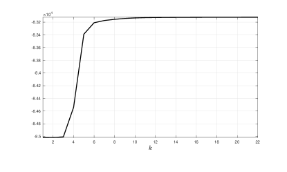
Figure 1: Expected log-likelihood

• This figure plots the value of the maximized expected conditional log-likelihood computed using the estimated factors, i.e., $\mathsf{E}_{\mathbf{\widehat{q}}^{\left(k\right)}}\left[\log f\left(\mathbf{X}\left|\widehat{\bm{G}};\widehat{\bm{\varphi}}^{(k+1)},\widehat{\bm{\rho}}^{(k+1)}\right.\right)\left|\bm{X}\right.\right]$ (see also (19)), as a function of the EM iterations $k$.

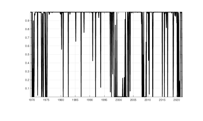
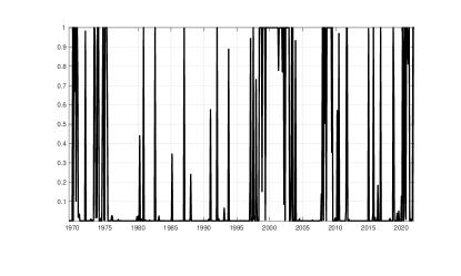
Figure 2: Estimated conditional probabilities $\widehat{\bm{\xi}}_{t|T}$.

(a): $\widehat{\xi}_{1,t|T}$	(b): $\widehat{\xi}_{2,t|T}$

• This figure plots the series of the estimated conditional probabilities $\widehat{\xi}_{1,t|T}$ (panel (a)) and $\widehat{\xi}_{2,t|T}$ (panel (b)), for $t=1,\ldots,T$, estimated from the Markov switching factor model in (13).

8.3 Factors and loadings - Linear factor model

Following the sequential order dictated by our estimation procedure, we first consider estimated factors and loadings for the equivalent linear representation in (14), namely the $N\times 2$ loadings matrix $\widehat{\mathbf{A}}$ with columns $\widehat{\mathbf{A}}_{j}$, $j=1,2$, having elements $\widehat{a}_{ji}$, $i=1,\ldots,N$, and the 2-dimensional vector of factors $\widehat{\mathbf{g}}_{t}=\left[\widehat{g}_{1t}\,\widehat{g}_{2t}\right]^{\prime}$, $t=1,\ldots,T$, both obtained via PCA as explained in Section 3.3. The estimated loadings are displayed in Figure 3 and the estimated factors are displayed in Figure 4.

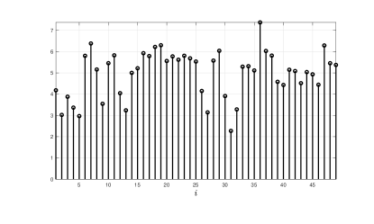
Figure 3: Estimated loadings $\widehat{\mathbf{A}}$ in the linear factor model.

(a): $\widehat{a}_{1i}$	(b): $\widehat{a}_{2i}$

• This figure plots the sequences of estimated loadings $\widehat{a}_{i1}$ (panel (a)) and $\widehat{a}_{i2}$ (panel (b)), for $i=1,\ldots,N$, estimated from the linear factor model in (14).

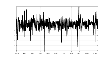
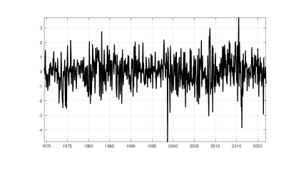
Figure 4: Estimated factors $\widehat{\mathbf{g}}_{t}$ in the linear factor model.

(a): $\widehat{g}_{1t}$	(b): $\widehat{g}_{2t}$

• This figure plots the series of the estimated factors $\widehat{g}_{1t}$ (panel (a)) and $\widehat{g}_{2t}$ (panel (b)), for $t=1,\ldots,T$, estimated from the linear factor model in (14).

The estimated loadings $\widehat{a}_{1i}$ associated to $\widehat{g}_{1t}$ all have the same sign. On the other hand, the loadings $\widehat{a}_{2i}$ associated to $\widehat{g}_{2t}$ have both positive and negative signs. To aid understanding of the factors, we study the correlation between them and the six observable factors considered in Fama and French (2016), namely: the value-weighted return on the market portfolio in excess of the one-month Treasury bill rate ($RM_{t}$); size ($SMB_{t}$); value ($HML_{t}$); profitability ($RMW_{t}$); investment ($CMA_{t}$); momentum ($MOM_{t}$). The correlations displayed in Table 5 show that the first estimated factor $\widehat{g}_{1t}$ is strongly correlated with the market return $RM_{t}$, it is reasonably correlated with $SMB_{t}$, $CMA_{t}$ and $MOM_{t}$, and it is only mildly correlated with $HML_{t}$ and $RMW_{t}$. On the other hand, the second estimated latent factor $\widehat{g}_{2t}$ does not exhibit any substantial correlation with any of the observable factors we consider. The first factor in the equivalent linear representation is then likely to be a market factor, while it is more difficult to give economic interpretation to the second factor.

Table 5: Factor correlations in the linear factor model.

	$\widehat{g}_{1t}$	$\widehat{g}_{2t}$
$RM_{t}$	0.96	0.05
$SMB_{t}$	0.40	-0.06
$HML_{t}$	-0.13	-0.06
$RMW_{t}$	-0.14	0.12
$CMA_{t}$	-0.32	-0.12
$MOM_{t}$	-0.26	-0.08

• This table reports the correlation coefficients between the estimated factors $\widehat{g}_{1t}$ and $\widehat{g}_{2t}$ from the equivalent linear specification in (14) and the following six observable factors from Fama and French (2016): the value-weighted return on the market portfolio in excess of the one-month Treasury bill rate ($RM_{t}$); size ($SMB_{t}$); value ($HML_{t}$); profitability ($RMW_{t}$); investment ($CMA_{t}$); momentum ($MOM_{t}$).

8.4 Factors and loadings - Markov switching factor model

We then turn to the estimated loadings and factors from the Markov switching factor model in (1). Since we have $r_{1}=r_{2}$, the estimators for $\bm{\Lambda}_{j}$, for $j=1,2$, are readily available from (46) or (47). Figure 5 shows the estimated loadings $\widehat{\lambda}_{1i}$ and $\widehat{\lambda}_{2i}$ (panels (a) and (b), respectively), and $\widetilde{\lambda}_{1i}$ and $\widetilde{\lambda}_{2i}$ (panels (c) and (d), respectively), for $i=1,\ldots,N$. As expected from Corollary 1, the two sets of estimators are similar, although not identical, since they are consistent for different linear transformations of the true loadings. In particular, the correlation between $\widehat{\lambda}_{1i}$ and $\widetilde{\lambda}_{1i}$ is $0.85$, whereas that between $\widehat{\lambda}_{2i}$ and $\widetilde{\lambda}_{2i}$ is $0.90$.

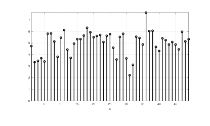
Figure 5: Estimated loadings $\widehat{\bm{\Lambda}}_{j}$ and $\widetilde{\bm{\Lambda}}_{j}$, $j=1,2$.

(a): $\widehat{\lambda}_{1i}$	(b): $\widehat{\lambda}_{2i}$
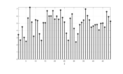
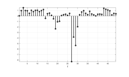
(c): $\widetilde{\lambda}_{1i}$	(d): $\widetilde{\lambda}_{2i}$

• This figure plots the sequences of estimated loadings $\widehat{\lambda}_{1i}$ (panel (a)), $\widehat{\lambda}_{2i}$ (panel (b)), $\widetilde{\lambda}_{1i}$ (panel (c)), and $\widetilde{\lambda}_{2i}$ (panel (d)), for $i=1,\ldots,N$, estimated from the Markov switching factor model in (1) according to (46) and (47).

Next, by projecting the data onto the estimated loadings weighted by the probability of being in a given state, we obtain the estimated scalar factors $\widehat{{f}}_{jt}$ and $\widetilde{{f}}_{jt}$, for $j=1,2$ and $t=1,\ldots,T$, as given in (48) and (49), respectively. These are shown in Figure 6. Finally, Table 6 displays the correlations between the estimated latent factors and the observable factors $RM_{t}$, $SMB_{t}$, $HML_{t}$, $RMW_{t}$, $CMA_{t}$, and $MOM_{t}$ described in Section 8.3. From the results in Table 6, we can see that $\widehat{{f}}_{1t}$, which estimates ${f}_{1t}$ according to (48), is strongly correlated with $RM_{t}$, and reasonably correlated with $SMB_{t}$, $HML_{t}$ and $CMA_{t}$. As for $\widehat{{f}}_{2t}$, the estimate for $f_{2t}$ from (48), it is correlated with $MOM_{t}$. A similar picture comes from $\widetilde{{f}}_{1t}$ and $\widetilde{{f}}_{2t}$, thus confirming the validity of our theoretical results.

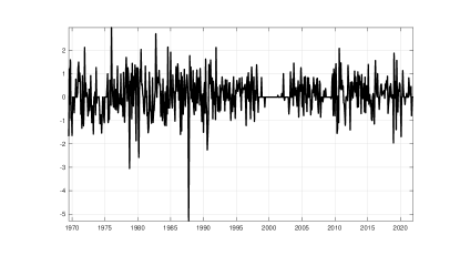
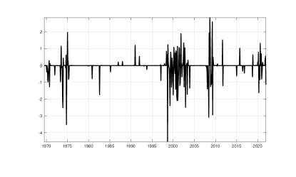
Figure 6: Estimated factors $\widehat{f}_{jt}$ and $\widetilde{f}_{jt}$, $j=1,2$.

(a): $\widehat{f}_{1t}$	(b): $\widehat{f}_{2t}$
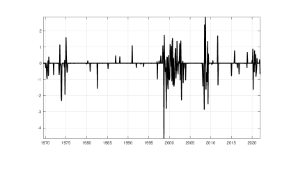
(c): $\widetilde{f}_{1t}$	(d): $\widetilde{f}_{2t}$

• This figure plots the series of the estimated factors $\widehat{f}_{1t}$ (panel (a)), $\widehat{f}_{2t}$ (panel (b)), $\widetilde{f}_{1t}$ (panel (c)), and $\widetilde{f}_{2t}$ (panel (d)), for $t=1,\dots,T$, estimated from the Markov switching factor model in (1) according to (48) and (49).

Table 6: Factor correlations in the Markov switching factor model.

	$\widehat{f}_{1t}$	$\widehat{f}_{2t}$	$\widetilde{f}_{1t}$	$\widetilde{f}_{2t}$
$RM_{t}$	0.74	0.01	0.74	-0.02
$SMB_{t}$	0.32	0.07	0.32	-0.03
$HML_{t}$	-0.17	0.06	-0.17	0.06
$RMW_{t}$	-0.06	0.02	-0.06	0.10
$CMA_{t}$	-0.22	-0.06	-0.13	-0.01
$MOM_{t}$	-0.01	-0.23	-0.01	-0.17

• This table reports the correlation coefficients between the estimated factors $\widehat{f}_{1t}$, $\widehat{f}_{2t}$, $\widetilde{f}_{1t}$, and $\widetilde{f}_{2t}$ from the Markov switching factor model in (1) according to (48) and (49), and the following six observable factors from Fama and French (2016): the value-weighted return on the market portfolio in excess of the one-month Treasury bill rate ($RM_{t}$); size ($SMB_{t}$); value ($HML_{t}$); profitability ($RMW_{t}$); investment ($CMA_{t}$); momentum ($MOM_{t}$).

9 Concluding remarks

This paper develops estimation and inferential theory for high dimensional factor models with discrete regime changes in the loadings driven by a latent first order Markov process. Our estimator employs a EM algorithm based on a modified version of the Baum-Lindgren-Hamilton-Kim filter and smoother. Remarkably, the estimator does not need knowledge of the number of factors in either states. It only requires the true number of factors in the equivalent linear representation, which can be estimated using existing techniques. We derive convergence rates and asymptotic distributions of the estimators for factors and loadings, and we show their good finite sample performance through an extensive set of Monte Carlo experiments. Finally, we empirically validate our methodology through an application to a large set of stock returns.

Our work can be extended along several dimensions. Two are worth mentioning. Our model allows for two regimes and the case of multiple states to capture richer dynamics is worth exploring. The challenging task of making inference on the number of regimes is also worth considering. These extensions are part of our research agenda.

Appendix A Details of estimation

A.1 Baum-Lindgren-Hamilton-Kim filter

For simplicity of notation, in this appendix we will consider both the factors $\{\mathbf{g}_{t}\}_{t=1}^{T}$ and the true values of the parameters $\mathbf{q}$ to be known. To simplify notation, let $\bm{\varepsilon}_{1}=\left[1\leavevmode\nobreak\ 0\right]^{\prime}$ and $\bm{\varepsilon}_{2}=\left[0\leavevmode\nobreak\ 1\right]^{\prime}$, so that $\mathsf{P}(s_{t}=j)\equiv\mathsf{P}(\bm{\xi}_{t}=\bm{\varepsilon}_{j})$, $j=1,2$, and therefore, in the following, we can just use $\bm{\xi}_{t}$ as defined in (4), without the need of referring also to $s_{t}$. Then, for any $v=1,\ldots,T$, we use the notation

$$\bm{\xi}_{t\left|v\right.}=\mathsf{E}\left[\bm{\xi}_{t}\left|\bm{X}_{v}\right.\right]=\left[\begin{array}[]{c}\mathsf{P}\left(\bm{\xi}_{t}=\bm{\varepsilon}_{1}\left|\bm{X}_{v}\right.\right)\\ \mathsf{P}\left(\bm{\xi}_{t}=\bm{\varepsilon}_{2}\left|\bm{X}_{v}\right.\right)\end{array}\right].$$ (A.1)

Notice also that, since $\{\bm{\xi}_{t}\}_{t=1}^{u}$ is independent of $\bm{G}_{v}$ for all $u,v=1,\ldots,T$, because we consider the factors as observed, we can always write $\bm{\xi}_{t\left|v\right.}=\mathsf{E}\left[\bm{\xi}_{t}\left|\bm{X}_{v}\right.\right]=\mathsf{E}\left[\bm{\xi}_{t}\left|\mathbf{X}_{v},\bm{G}_{v}\right.\right]$.

The one-step-ahead predictions and the filtered probabilities are computed by means of the following steps which are similar to the Hamilton filter, see, e.g., Krolzig (2013, Chapter 5.1) and Hamilton (1989).

Then, the one-step-ahead predicted probabilities are obtained through the prior probability

$$\mathsf{P}\left(\bm{\xi}_{t}=\bm{\varepsilon}_{i}\left|\bm{X}_{t-1},\bm{G}_{t-1}\right.\right) =\sum\limits_{j=1}^{2}\mathsf{P}\left(\bm{\xi}_{t}=\bm{\varepsilon}_{i}\left|\bm{\xi}_{t-1}=\bm{\varepsilon}_{j}\right.\right)\mathsf{P}\left(\bm{\xi}_{t-1}=\bm{\varepsilon}_{j}\left|\bm{X}_{t-1},\bm{G}_{t-1}\right.\right)$$

$$=\sum\limits_{j=1}^{2}\mathsf{P}\left(\bm{\xi}_{t}=\bm{\varepsilon}_{i}\left|\bm{\xi}_{t-1}=\bm{\varepsilon}_{j}\right.\right)\mathsf{P}\left(\bm{\xi}_{t-1}=\bm{\varepsilon}_{j}\left|\bm{X}_{t-1}\right.\right),\qquad i=1,2.$$ (A.2)

So that, because of (A.1), we have

$$\bm{\xi}_{t\left|t-1\right.}=\mathbf{P}^{\prime}\bm{\xi}_{t-1\left|t-1\right.},\quad t=1,\ldots,T.$$ (A.3)

The update involves the posterior probability:

$$\mathsf{P}\left(\bm{\xi}_{t}=\bm{\varepsilon}_{i}\left|\bm{X}_{t}\right.\right) =\mathsf{P}\left(\bm{\xi}_{t}=\bm{\varepsilon}_{i}\left|\bm{X}_{t},\bm{G}_{t}\right.\right)=\mathsf{P}\left(\bm{\xi}_{t}=\bm{\varepsilon}_{i}\left|\mathbf{x}_{t},\bm{X}_{t-1},\bm{G}_{t}\right.\right)$$

$$=\dfrac{f\left(\mathbf{x}_{t},\bm{\xi}_{t}=\bm{\varepsilon}_{i}\left|\bm{X}_{t-1},\bm{G}_{t}\right.\right)}{f\left(\mathbf{x}_{t}\left|\bm{X}_{t-1},\bm{G}_{t}\right.\right)}$$

$$=\dfrac{f\left(\mathbf{x}_{t}\left|\bm{\xi}_{t}=\bm{\varepsilon}_{i},\bm{X}_{t-1},\bm{G}_{t}\right.\right)\mathsf{P}\left(\bm{\xi}_{t}=\bm{\varepsilon}_{i}\left|\bm{X}_{t-1},\bm{G}_{t}\right.\right)}{f\left(\mathbf{x}_{t}\left|\bm{X}_{t-1},\bm{G}_{t}\right.\right)},\quad i=1,2.$$ (A.4)

Then, since $\mathbf{x}_{t}$ depends on $\bm{X}_{t-1}$ only through $\bm{\xi}_{t-1}$ and it depends on $\bm{G}_{t}$ only through $\mathbf{g}_{t}$

$$f\left(\mathbf{x}_{t}\left|\bm{\xi}_{t}=\bm{\varepsilon}_{i},\bm{X}_{t-1},\bm{G}_{t}\right.\right)=f\left(\mathbf{x}_{t}\left|\bm{\xi}_{t}=\bm{\varepsilon}_{i},\mathbf{g}_{t}\right.\right),\quad i=1,2.$$ (A.5)

Let,

$$\bm{\eta}_{t} =\left[\begin{array}[]{c}f\left(\mathbf{x}_{t}\left|\bm{\xi}_{t}=\bm{\varepsilon}_{1},\mathbf{{g}}_{t}\right.\right)\\ f\left(\mathbf{x}_{t}\left|\bm{\xi}_{t}=\bm{\varepsilon}_{2},\mathbf{{g}}_{t}\right.\right)\end{array}\right]$$ (A.8)

$$=\dfrac{1}{\left(2\pi\right)^{N\left/2\right.}}\left\{\begin{array}[]{c}\left|\text{diag}(\bm{\Sigma}_{e1})\right|^{-1\left/2\right.}\exp\left[-\dfrac{1}{2}\left(\mathbf{x}_{t}-\mathbf{B}_{1}\mathbf{{g}}_{t}\right)^{\prime}\left(\text{diag}(\bm{\Sigma}_{e1})\right)^{-1}\left(\mathbf{x}_{t}-\mathbf{B}_{1}\mathbf{{g}}_{t}\right)\right]\\ \\ \left|\text{diag}(\bm{\Sigma}_{e2})\right|^{-1\left/2\right.}\exp\left[-\dfrac{1}{2}\left(\mathbf{x}_{t}-\mathbf{B}_{2}\mathbf{{g}}_{t}\right)^{\prime}\left(\text{diag}(\bm{\Sigma}_{e2})\right)^{-1}\left(\mathbf{x}_{t}-\mathbf{B}_{2}\mathbf{{g}}_{t}\right)\right]\end{array}\right\}.$$ (A.12)

Further, notice that, from (A.1) and (A.12), the denominator of (A.4) be written as:

$$f\left(\mathbf{x}_{t}\left|\bm{X}_{t-1},\bm{G}_{t}\right.\right) =\sum\limits_{j=1}^{2}f\left(\mathbf{x}_{t}\left|\bm{\xi}_{t}=\bm{\varepsilon}_{j},\bm{X}_{t-1},\bm{G}_{t}\right.\right)\mathsf{P}\left(\bm{\xi}_{t}=\bm{\varepsilon}_{j},\left|\bm{X}_{t-1},\bm{G}_{t}\right.\right)$$

$$=\sum\limits_{j=1}^{2}f\left(\mathbf{x}_{t}\left|\bm{\xi}_{t}=\bm{\varepsilon}_{j},\mathbf{g}_{t}\right.\right)\mathsf{P}\left(\bm{\xi}_{t}=\bm{\varepsilon}_{j},\left|\bm{X}_{t-1}\right.\right)=\bm{\eta}_{t}^{\prime}\bm{\xi}_{t\left|t-1\right.}.$$ (A.13)

Taking into account (A.1), (A.2), (A.5), and (A.13), the filtered probabilities are obtained from (A.4) as

$$\bm{\xi}_{t\left|t\right.}=\dfrac{\bm{\eta}_{t}\odot\bm{\xi}_{t\left|t-1\right.}}{\bm{\eta}_{t}^{\prime}\bm{\xi}_{t\left|t-1\right.}}=\dfrac{\bm{\eta}_{t}\odot\bm{\xi}_{t\left|t-1\right.}}{\bm{\iota}_{2}^{\prime}\left(\bm{\eta}_{t}\odot\bm{\xi}_{t\left|t-1\right.}\right)},\quad t=1,\ldots,T,$$ (A.14)

where $\bm{\eta}_{t}$ is computed as in (A.12). The filter can started by setting either $\bm{\xi}_{0|0}=\bm{\varepsilon}_{1}$, or, equivalently, $\bm{\xi}_{0|0}=\bm{\varepsilon}_{2}$.

We then run the Kim smoother, see e.g., Krolzig (2013, Chapter 5.2) and Kim (1994). Notice that (recall that $\bm{X}\equiv\bm{X}_{T}$ and $\bm{G}\equiv\bm{{G}}_{T}$):

$$\mathsf{P} \left(\bm{\xi}_{t}=\bm{\varepsilon}_{i}\left|\bm{X},\bm{{G}}\right.\right)=\sum_{j=1}^{2}\mathsf{P}\left(\bm{\xi}_{t}=\bm{\varepsilon}_{i}\left|\bm{\xi}_{t+1}=\bm{\varepsilon}_{j},\bm{X},\bm{{G}}\right.\right)\mathsf{P}\left(\bm{\xi}_{t+1}=\bm{\varepsilon}_{j}\left|\bm{X},\bm{{G}}\right.\right)$$

$$=\sum_{j=1}^{2}\dfrac{\mathsf{P}\left(\bm{\xi}_{t}=\bm{\varepsilon}_{i}\left|\bm{\xi}_{t+1}=\bm{\varepsilon}_{j},\bm{X}_{t},\bm{{G}}_{t}\right.\right)f\left(\left\{\mathbf{x}_{s},\mathbf{{g}}_{s}\right\}_{s=t+1}^{T}\left|\bm{\xi}_{t}=\bm{\varepsilon}_{i},\bm{\xi}_{t+1}=\bm{\varepsilon}_{j},\bm{X}_{t},\bm{G}_{t}\right.\right)}{f\left(\left\{\mathbf{x}_{s},\mathbf{{g}}_{s}\right\}_{s=t+1}^{T}\left|\bm{\xi}_{t+1}=\bm{\varepsilon}_{j},\bm{X}_{t},\bm{{G}}_{t}\right.\right)}\mathsf{P}\left(\bm{\xi}_{t+1}=\bm{\varepsilon}_{j}\left|\bm{X},\bm{{G}}\right.\right)$$

$$=\sum_{j=1}^{2}\mathsf{P}\left(\bm{\xi}_{t}=\bm{\varepsilon}_{i}\left|\bm{\xi}_{t+1}=\bm{\varepsilon}_{j},\bm{X}_{t},\bm{{G}}_{t}\right.\right)\mathsf{P}\left(\bm{\xi}_{t+1}=\bm{\varepsilon}_{j}\left|\bm{X},\bm{{G}}\right.\right)$$

$$=\sum_{j=1}^{2}\dfrac{\mathsf{P}\left(\bm{\xi}_{t}=\bm{\varepsilon}_{i}\left|\bm{X}_{t},\bm{{G}}_{t}\right.\right)\mathsf{P}\left(\bm{\xi}_{t+1}=\bm{\varepsilon}_{j}\left|\bm{\xi}_{t}=\bm{\varepsilon}_{i},\bm{X}_{t},\bm{{G}}_{t}\right.\right)}{\mathsf{P}\left(\bm{\xi}_{t+1}=\bm{\varepsilon}_{j}\left|\bm{X}_{t},\bm{{G}}_{t}\right.\right)}\mathsf{P}\left(\bm{\xi}_{t+1}=\bm{\varepsilon}_{j}\left|\bm{X},\bm{{G}}\right.\right),\quad i=1,2,$$

which by (A.1) implies that the sequence of smoothed probabilities is given by

$$\bm{\xi}_{t\left|T\right.}=\left[\mathbf{P}\left(\bm{\xi}_{t+1\left|T\right.}\oslash\bm{\xi}_{t+1\left|t\right.}\right)\right]\odot\bm{\xi}_{t\left|t\right.},\quad t=1,\ldots,T.$$ (A.15)

This backward recursion is initiated at $\bm{\xi}_{T|T}$ which is the last iteration of the filter in (A.14).

Finally, for the implementation of the EM algorithm we need to compute also the smoothed cross-probabilities, see Krolzig (2013, Chapter 5.A.2),

$$\bm{\xi}_{t,t-1|T}=\left[\begin{array}[]{c}\mathsf{P}(\bm{\xi}_{t}=\bm{\varepsilon}_{1},\bm{\xi}_{t-1}=\bm{\varepsilon}_{1}|\bm{X})\\ \mathsf{P}(\bm{\xi}_{t}=\bm{\varepsilon}_{2},\bm{\xi}_{t-1}=\bm{\varepsilon}_{1}|\bm{X})\\ \mathsf{P}(\bm{\xi}_{t}=\bm{\varepsilon}_{1},\bm{\xi}_{t-1}=\bm{\varepsilon}_{2}|\bm{X})\\ \mathsf{P}(\bm{\xi}_{t}=\bm{\varepsilon}_{2},\bm{\xi}_{t-1}=\bm{\varepsilon}_{2}|\bm{X})\end{array}\right]=\bm{\rho}\,\odot\left[\left(\bm{\xi}_{t|T}\oslash\bm{\xi}_{t|t-1}\right)\otimes\bm{\xi}_{t-1|t-1}\right],\quad t=1,\ldots,T.$$ (A.16)

A.2 M-step

In the M step we have to solve the constrained maximization problem in (19). Let us start with estimation of $\bm{\varphi}$. From (16), we have:

$$\frac{\partial\log f\left(\mathbf{X}\left|\bm{G};\bm{\varphi},\bm{\rho}\right.\right)}{\partial\bm{\varphi}^{\prime}}=\frac{1}{f\left(\mathbf{X}\left|\bm{G};\bm{\varphi},\bm{\rho}\right.\right)}\sum_{\{\bm{\xi}_{t}\}_{t=1}^{T}}\frac{\partial f\left(\mathbf{X}\left|\bm{G},\{\bm{\xi}_{t}\}_{t=1}^{T};\bm{\varphi}\right.\right)}{\partial\bm{\varphi}^{\prime}}\mathsf{P}\left(\{\bm{\xi}_{t}\}_{t=1}^{T}|\bm{G},\bm{\rho}\right)$$

$$=\frac{1}{f\left(\mathbf{X}\left|\bm{G};\bm{\varphi},\bm{\rho}\right.\right)}\sum_{\{\bm{\xi}_{t}\}_{t=1}^{T}}\frac{\partial\log f\left(\mathbf{X}\left|\bm{G},\{\bm{\xi}_{t}\}_{t=1}^{T};\bm{\varphi}\right.\right)}{\partial\bm{\varphi}^{\prime}}f\left(\mathbf{X}\left|\bm{G},\{\bm{\xi}_{t}\}_{t=1}^{T};\bm{\varphi}\right.\right)\mathsf{P}\left(\{\bm{\xi}_{t}\}_{t=1}^{T}|\bm{G};\bm{\rho}\right)$$

$$=\mathcal{C}\sum_{\{\bm{\xi}_{t}\}_{t=1}^{T}}\frac{\partial\log f\left(\mathbf{X}\left|\bm{G},\{\bm{\xi}_{t}\}_{t=1}^{T};\bm{\varphi}\right.\right)}{\partial\bm{\varphi}^{\prime}}\mathsf{P}\left(\{\bm{\xi}_{t}\}_{t=1}^{T}|\bm{X},\bm{G};\bm{\varphi},\bm{\rho}\right),$$ (A.17)

where $\mathcal{C}$ is a positive normalization constant. Therefore, from (17), (19), and (A.17), if we observed $\bm{G}$, the first order conditions would be:

$$\mathbf{0} =\left.\frac{\partial\mathsf{E}_{\widehat{\mathbf{q}}^{(k)}}\left[\log f\left(\mathbf{X}\left|\bm{G};\bm{\varphi},\bm{\rho}\right.\right)\left|\bm{X}\right.\right]}{\partial\bm{\varphi}^{\prime}}\right|_{\bm{\varphi}=\widehat{\bm{\varphi}}^{(k+1)}}$$

$$=\sum_{t=1}^{T}\sum_{j=1}^{2}\left.\frac{\partial\mathsf{E}_{\widehat{\mathbf{q}}^{(k)}}\left[\log f\left(\mathbf{x}_{t}\left|\mathbf{g}_{t},\bm{\xi}_{t}=\bm{\varepsilon}_{j};\bm{\varphi}\right.\right)\left|\bm{X}\right.\right]}{\partial\bm{\varphi}^{\prime}}\right|_{\bm{\varphi}=\widehat{\bm{\varphi}}^{(k+1)}}\mathsf{P}\left(\bm{\xi}_{t}=\bm{\varepsilon}_{j}|\bm{X};\widehat{\bm{\varphi}}^{(k)},\widehat{\bm{\rho}}^{(k)}\right)$$

$$=\sum_{t=1}^{T}\sum_{j=1}^{2}\left.\frac{\partial\mathsf{E}_{\widehat{\mathbf{q}}^{(k)}}\left[\log f\left(\mathbf{x}_{t}\left|\mathbf{g}_{t},\bm{\xi}_{t}=\bm{\varepsilon}_{j};\bm{\varphi}\right.\right)\left|\bm{X}\right.\right]}{\partial\bm{\varphi}^{\prime}}\right|_{\bm{\varphi}=\widehat{\bm{\varphi}}^{(k+1)}}\xi_{j,t|T}^{(k)},$$ (A.18)

where ${\xi}_{j,t\left|T\right.}^{(k)}=\mathsf{E}_{\widehat{\mathbf{q}}^{(k)}}[\xi_{jt}|\mathbf{X}]=\mathsf{P}(\bm{\xi}_{t}=\bm{\varepsilon}_{j}\left|\bm{X};\widehat{\bm{\varphi}}^{(k)},\widehat{\bm{\rho}}^{(k)}\right.)$ is the $j$th component of $\bm{\xi}_{t\left|T\right.}^{(k)}$.

Then, by substituting (17) into (A.18), and by replacing true factors with estimated ones, we get

$$\mathbf{\widehat{B}}_{j}^{(k+1)}=\left(\sum_{t=1}^{T}{\xi}_{j,t\left|T\right.}^{(k)}\mathbf{x}_{t}\mathbf{\widehat{g}}_{t}^{\prime}\right)\left(\sum_{t=1}^{T}{\xi}_{j,t\left|T\right.}^{(k)}\widehat{\mathbf{g}}_{t}\mathbf{\widehat{g}}_{t}^{\prime}\right)^{-1},\quad j=1,2,$$ (A.19)

and, consistently with the fact that we use a mis-specified likelihood with uncorrelated idiosyncratic components, we set

$$[\widehat{\mathbf{\Sigma}}_{ej}^{(k+1)}]_{ii} =\left(\dfrac{\sum_{t=1}^{T}\left({x}_{it}-\mathbf{\widehat{b}}_{ji}^{(k+1)\prime}\mathbf{\widehat{g}}_{t}\right)^{2}}{\sum_{t=1}^{T}{\xi}_{j,t\left|T\right.}^{(k)}}\right),\quad i=1,\ldots,N,\quad j=1,2,$$ (A.20)

$$[\widehat{\mathbf{\Sigma}}_{ej}^{(k+1)}]_{ik} =0,\quad i,k=1,\ldots,N,\quad i\neq k,\quad j=1,2,$$

where $\mathbf{\widehat{b}}_{ji}^{(k+1)\prime}$ is the $i$th row of $\mathbf{\widehat{B}}_{j}^{(k+1)}$.

Moving to estimation of $\bm{\rho}$, from (16), we have:

$$\frac{\partial\log f\left(\mathbf{X}\left|\bm{G};\bm{\varphi},\bm{\rho}\right.\right)}{\partial\bm{\rho}^{\prime}}=\frac{1}{f\left(\mathbf{X}\left|\bm{G};\bm{\varphi},\bm{\rho}\right.\right)}\sum_{\{\bm{\xi}_{t}\}_{t=1}^{T}}f\left(\mathbf{X}\left|\bm{G},\{\bm{\xi}_{t}\}_{t=1}^{T};\bm{\varphi}\right.\right)\frac{\partial\mathsf{P}\left(\{\bm{\xi}_{t}\}_{t=1}^{T}|\bm{G};\bm{\rho}\right)}{\partial\bm{\rho}^{\prime}}$$

$$=\frac{1}{f\left(\mathbf{X}\left|\bm{G};\bm{\varphi},\bm{\rho}\right.\right)}\sum_{\{\bm{\xi}_{t}\}_{t=1}^{T}}\frac{\partial\log\mathsf{P}\left(\{\bm{\xi}_{t}\}_{t=1}^{T}|\bm{G};\bm{\rho}\right)}{\partial\bm{\rho}^{\prime}}f\left(\mathbf{X}\left|\bm{G},\{\bm{\xi}_{t}\}_{t=1}^{T};\bm{\varphi}\right.\right)\mathsf{P}\left(\{\bm{\xi}_{t}\}_{t=1}^{T}|\bm{G};\bm{\rho}\right)$$

$$=\mathcal{C}\sum_{\{\bm{\xi}_{t}\}_{t=1}^{T}}\frac{\partial\log\mathsf{P}\left(\{\bm{\xi}_{t}\}_{t=1}^{T}|\bm{G};\bm{\rho}\right)}{\partial\bm{\rho}^{\prime}}\mathsf{P}\left(\{\bm{\xi}_{t}\}_{t=1}^{T}|\bm{X},\bm{G};\bm{\varphi},\bm{\rho}\right),$$ (A.21)

where $\mathcal{C}$ is the same positive normalization constant as in (A.17). And, because of (18) and (A.21), if we observed $\bm{G}$ the derivatives with respect to the generic $(i,j)$th element of $\bm{\rho}$, i.e, $p_{ij}$, $i,j=1,2$, would be (treating $\bm{\xi}_{0}$ as known)

$$\frac{\partial\log f\left(\mathbf{X}\left|\bm{G};\bm{\varphi},\bm{\rho}\right.\right)}{\partial p_{ij}}$$

$$=\sum_{t=1}^{T}\sum_{h=1}^{2}\sum_{\ell=1}^{2}\frac{\partial\log\mathsf{P}\left(\bm{\xi}_{t}=\bm{\varepsilon}_{h}|\bm{\xi}_{t-1}=\bm{\varepsilon}_{\ell};\bm{\rho}\right)}{\partial p_{ij}}\mathsf{P}\left(\bm{\xi}_{t}=\bm{\varepsilon}_{h},\bm{\xi}_{t-1}=\bm{\varepsilon}_{\ell}|\bm{X};{\bm{\varphi}},{\bm{\rho}}\right)$$

$$=\sum_{t=1}^{T}\sum_{h=1}^{2}\sum_{\ell=1}^{2}\frac{1}{\mathsf{P}\left(\bm{\xi}_{t}=\bm{\varepsilon}_{h}|\bm{\xi}_{t-1}=\bm{\varepsilon}_{\ell};\bm{\rho}\right)}\frac{\partial\mathsf{P}\left(\bm{\xi}_{t}=\bm{\varepsilon}_{h}|\bm{\xi}_{t-1}=\bm{\varepsilon}_{\ell};\bm{\rho}\right)}{\partial p_{ij}}\mathsf{P}\left(\bm{\xi}_{t}=\bm{\varepsilon}_{h},\bm{\xi}_{t-1}=\bm{\varepsilon}_{\ell}|\bm{X};{\bm{\varphi}},{\bm{\rho}}\right)$$

$$=\sum_{t=1}^{T}\sum_{h=1}^{2}\sum_{\ell=1}^{2}\frac{\mathbb{I}\left(\bm{\xi}_{t}=\bm{\varepsilon}_{j},\bm{\xi}_{t-1}=\bm{\varepsilon}_{i}\right)}{\mathsf{P}\left(\bm{\xi}_{t}=\bm{\varepsilon}_{h}|\bm{\xi}_{t-1}=\bm{\varepsilon}_{\ell};\bm{\rho}\right)}\mathsf{P}\left(\bm{\xi}_{t}=\bm{\varepsilon}_{h},\bm{\xi}_{t-1}=\bm{\varepsilon}_{\ell}|\bm{X};{\bm{\varphi}},{\bm{\rho}}\right)$$

$$=\sum_{t=1}^{T}\frac{\mathsf{P}\left(\bm{\xi}_{t}=\bm{\varepsilon}_{j},\bm{\xi}_{t-1}=\bm{\varepsilon}_{i}|\bm{X};{\bm{\varphi}},{\bm{\rho}}\right)}{\mathsf{P}\left(\bm{\xi}_{t}=\bm{\varepsilon}_{j}|\bm{\xi}_{t-1}=\bm{\varepsilon}_{i};\bm{\rho}\right)}=\sum_{t=1}^{T}\frac{\mathsf{P}\left(\bm{\xi}_{t}=\bm{\varepsilon}_{j},\bm{\xi}_{t-1}=\bm{\varepsilon}_{i}|\bm{X};{\bm{\varphi}},{\bm{\rho}}\right)}{p_{ij}}.$$ (A.22)

Now, from (19) and (A.21), the first order conditions are:

$$\mathbf{0}= \left.\left\{\frac{\partial\mathsf{E}_{\widehat{\mathbf{q}}^{(k)}}\left[\log f\left(\mathbf{X}\left|\bm{G};\bm{\varphi},\bm{\rho}\right.\right)\left|\bm{X}\right.\right]}{\partial(\text{vec}(\mathbf{P}))^{\prime}}-\bm{\kappa}^{\prime}\left(\bm{\iota}_{2}^{\prime}\otimes\mathbf{I}_{2}\right)\right\}\right|_{\text{vec}(\mathbf{P})=\text{vec}(\widehat{\mathbf{P}}^{(k+1)})},$$ (A.23)

where $\bm{\kappa}$ is the $2$-dimensional vector of Lagrange multipliers, thus it has positive entries. Then, from (A.22)

$$\frac{\partial\mathsf{E}_{\widehat{\mathbf{q}}^{(k)}}\left[\log f\left(\mathbf{X}\left|\bm{G};\bm{\varphi},\bm{\rho}\right.\right)\left|\bm{X}\right.\right]}{\partial p_{ij}} =\sum_{t=1}^{T}\frac{\mathsf{P}\left(\bm{\xi}_{t}=\bm{\varepsilon}_{j},\bm{\xi}_{t-1}=\bm{\varepsilon}_{i}|\bm{X};\widehat{\bm{\varphi}}^{(k)},\widehat{\bm{\rho}}^{(k)}\right)}{p_{ij}}.$$ (A.24)

By collecting all 4 terms deriving from (A.24) into a vector, we have

$$\frac{\partial\mathsf{E}_{\widehat{\mathbf{q}}^{(k)}}\left[\log f\left(\mathbf{X}\left|\bm{G};\bm{\varphi},\bm{\rho}\right.\right)\left|\bm{X}\right.\right]}{\partial\bm{\rho}^{\prime}} =\sum_{t=1}^{T}\bm{\xi}_{t,t-1|T}^{(k)\prime}\oslash\bm{\rho}^{\prime},$$ (A.25)

where $\bm{\xi}_{t,t-1|T}^{(k)}$ is defined in (A.16). Finally, from the first order conditions (A.23), we must have:

$$\mathbf{0}=\left.\left\{\sum_{t=1}^{T}\bm{\xi}_{t,t-1|T}^{(k)\prime}\oslash\bm{\rho}^{\prime}-\bm{\kappa}^{\prime}\left(\bm{\iota}_{2}^{\prime}\otimes\mathbf{I}_{2}\right)\right\}\right|_{\bm{\rho}=\widehat{\bm{\rho}}^{(k+1)}}.$$ (A.26)

Let $\bm{\kappa}=(\kappa_{1},\kappa_{2})^{\prime}$, and let $\widetilde{\bm{\kappa}}=\left(\bm{\iota}_{2}\otimes\bm{\kappa}\right)=(\kappa_{1},\kappa_{2},\kappa_{1},\kappa_{2})^{\prime}$. Then, (A.26) gives

$$\widehat{\bm{\rho}}^{(k+1)}=\sum_{t=1}^{T}\bm{\xi}_{t,t-1|T}^{(k)}\oslash\widetilde{\bm{\kappa}}.$$ (A.27)

By applying the adding up condition to (A.27):

$$\bm{\iota}_{2} =\left(\bm{\iota}_{2}^{\prime}\otimes\mathbf{I}_{2}\right)\widehat{\bm{\rho}}^{(k+1)}=\left(\bm{\iota}_{2}^{\prime}\otimes\mathbf{I}_{2}\right)\left(\sum_{t=1}^{T}\bm{\xi}_{t,t-1|T}^{(k)}\oslash\widetilde{\bm{\kappa}}\right)=\left(\bm{\iota}_{2}^{\prime}\otimes\mathbf{I}_{2}\right)\sum_{t=1}^{T}\left(\begin{array}[]{c}\frac{\xi_{11,t,t-1|T}^{(k)}}{\kappa_{1}}\\ \frac{\xi_{21,t,t-1|T}^{(k)}}{\kappa_{2}}\\ \frac{\xi_{12,t,t-1|T}^{(k)}}{\kappa_{1}}\\ \frac{\xi_{22,t,t-1|T}^{(k)}}{\kappa_{2}}\end{array}\right)$$ (A.32)

$$=\sum_{t=1}^{T}\sum_{j=1}^{2}\left(\begin{array}[]{c}\frac{\xi_{1j,t,t-1|T}^{(k)}}{\kappa_{1}}\\ \frac{\xi_{2j,t,t-1|T}^{(k)}}{\kappa_{2}}\end{array}\right)=\sum_{t=1}^{T}\left(\begin{array}[]{c}\frac{\xi_{1,t-1|T}^{(k)}}{\kappa_{1}}\\ \frac{\xi_{2,t-1|T}^{(k)}}{\kappa_{2}}\end{array}\right)=\sum_{t=0}^{T-1}\left(\begin{array}[]{c}\frac{\xi_{1,t|T}^{(k)}}{\kappa_{1}}\\ \frac{\xi_{2,t|T}^{(k)}}{\kappa_{2}}\end{array}\right)=\sum_{t=0}^{T-1}\bm{\xi}_{t|T}^{(k)}\oslash{\bm{\kappa}},$$ (A.39)

which implies ${\bm{\kappa}}=\sum_{t=0}^{T-1}\bm{\xi}_{t|T}^{(k)}$. Therefore, from (A.27),

$$\widehat{\bm{\rho}}^{(k+1)}=\left[\sum_{t=1}^{T}\bm{\xi}_{t,t-1|T}^{(k)}\right]\oslash\left[\bm{\iota}_{2}\otimes\sum_{t=0}^{T-1}\bm{\xi}_{t|T}^{(k)}\right].$$ (A.40)

Appendix B Mathematical proofs

Define $C_{NT}=\min\left\{\sqrt{N},\sqrt{T}\right\}$ Let $\mathbb{I}_{1t}=\mathbb{I}(s_{t}=1)$ and $\mathbb{I}_{2t}=\mathbb{I}(s_{t}=2)$. For $j=1,2$, and $i,l=1,\ldots,N$, define

$$\begin{array}[]{rl}\sigma_{jil}=\mathsf{E}\left(\dfrac{1}{T}\sum\limits_{t=1}^{T}\mathbb{I}_{jt}e_{it}e_{lt}\right),&\chi_{jil}=\dfrac{1}{T}\sum\limits_{t=1}^{T}\mathbb{I}_{jt}e_{it}e_{lt}-\mathsf{E}\left(\dfrac{1}{T}\sum\limits_{t=1}^{T}\mathbb{I}_{jt}e_{it}e_{lt}\right),\\ \varphi_{jil}=\dfrac{1}{T}\sum\limits_{t=1}^{T}\mathbb{I}_{jt}\bm{\lambda}_{ji}^{\prime}\mathbf{f}_{jt}e_{lt},&\varphi_{jli}=\dfrac{1}{T}\sum\limits_{t=1}^{T}\mathbb{I}_{jt}\bm{\lambda}_{jl}^{\prime}\mathbf{f}_{jt}e_{it}.\end{array}$$ (B.1)

B.1 Lemmas

Lemma 1.

Under Assumptions 1 - 4, and given $\mathbf{\widehat{H}}$ defined in $\left(\ref{eq:hat_H}\right)$, we have

$$\dfrac{1}{N}\sum\limits_{i=1}^{N}\left\|\mathbf{\widehat{a}}_{i}-\mathbf{\widehat{H}}^{\prime}\mathbf{a}_{i}\right\|^{2}=O_{p}\left(\dfrac{1}{C_{NT}^{2}}\right).$$

Lemma 2.

Let Assumptions 1 - 6 hold. Then:

(a)

$N^{-1}\sum\nolimits_{l=1}^{N}\mathbf{\widehat{a}}_{l}\sigma_{jil}=O_{p}\left(\tfrac{1}{\sqrt{N}C_{NT}}\right)$;

(b)

$N^{-1}\sum\nolimits_{l=1}^{N}\mathbf{\widehat{a}}_{l}\chi_{jil}=O_{p}\left(\tfrac{1}{\sqrt{T}C_{NT}}\right)$;

(c)

$N^{-1}\sum\nolimits_{l=1}^{N}\mathbf{\widehat{a}}_{l}\varphi_{jil}=O_{p}\left(\tfrac{1}{\sqrt{T}C_{NT}}\right)$;

(d)

$N^{-1}\sum\nolimits_{l=1}^{N}\mathbf{\widehat{a}}_{l}\varphi_{jli}=O_{p}\left(\tfrac{1}{\sqrt{T}}\right)$.

Lemma 3.

Under Assumptions 1 - 6,

$$N^{-1}\left(\mathbf{\widehat{A}}-\mathbf{A\widehat{H}}\right)^{\prime}\mathbf{\widehat{A}}=O_{p}\left(\dfrac{1}{C_{NT}^{2}}\right).$$

Lemma 4.

Under Assumptions 1 - 6,

$$N^{-1}\left(\mathbf{\widehat{A}}-\mathbf{A\widehat{H}}\right)^{\prime}\mathbf{e}_{t}=O_{p}\left(\dfrac{1}{C^{2}_{NT}}\right).$$

Lemma 5.

Let Assumptions 1 - 6 hold. Then:

(a)

$\mathbf{\widehat{g}}_{t}-\mathbf{\widehat{H}}^{-1}\mathbf{g}_{t}=O_{p}\left(\tfrac{1}{\sqrt{N}}\right)+O_{p}\left(\tfrac{1}{C_{NT}^{2}}\right)$, for $t=1,\dots,T$;

(b)

$\tfrac{1}{T}\sum\nolimits_{t=1}^{T}\left(\mathbf{\widehat{g}}_{t}-\widehat{\mathbf{H}}^{-1}\mathbf{g}_{t}\right)\mathbf{\widehat{g}}_{t}^{\prime}=O_{p}\left(\tfrac{1}{C_{NT}^{2}}\right).$

Lemma 6.

Under Assumptions 1 - 5, and given $\mathbf{Q}$ defined in (39),

$$p\lim_{N,T\rightarrow\infty}\dfrac{\mathbf{A}^{\prime}\mathbf{\widehat{A}}}{N}=\mathbf{Q}.$$

Lemma 7.

Let Assumptions 1 - 5 hold, and consider the matrix $\mathbf{Q}$ defined in (39). Then, for $j=1,2$, the $r_{j}\times\left(r_{1}+r_{2}\right)$ matrix $\mathbf{Q}_{j}$ satisfying $\mathbf{Q}=\left[\mathbf{Q}_{1}^{\prime}\ \mathbf{Q}_{2}^{\prime}\right]^{\prime}$ is such that

$$\mathbf{Q}_{j}=\mathbf{\Sigma}_{\mathbf{f}j}^{-1\left/2\right.}\mathbf{\Psi}_{j}\mathbf{V}^{1\left/2\right.},$$

where $\mathbf{\Sigma}_{\mathbf{f}j}$ is defined in (29), and $\mathbf{\Psi}_{j}$ is the $r_{j}\times\left(r_{1}+r_{2}\right)$ matrix such that $\mathbf{\Psi}=\left[\mathbf{\Psi}_{1}^{\prime}\ \mathbf{\Psi}_{2}^{\prime}\right]^{\prime}$, with $\mathbf{\Psi}$ as in (39).

Lemma 8.

Let $\mathbf{\widehat{V}}$ be the $\left(r_{1}+r_{2}\right)\times\left(r_{1}+r_{2}\right)$ diagonal matrix containing the first $r_{1}+r_{2}$ eigenvalues of $\mathbf{\widehat{\Sigma}}_{\mathbf{x}}=\left(NT\right)^{-1}\sum\nolimits_{t=1}^{T}\mathbf{x}_{t}\mathbf{x}_{t}^{\prime}$ in decreasing order. Define $\mathbf{V}$ as the $\left(r_{1}+r_{2}\right)\times\left(r_{1}+r_{2}\right)$ diagonal matrix of the first $r_{1}+r_{2}$ eigenvalues of $\mathbf{\Sigma}_{\mathbf{g}}^{1\left/2\right.}\mathbf{\Sigma}_{\mathbf{A}}\mathbf{\Sigma}_{\mathbf{g}}^{1\left/2\right.}$ in decreasing order, where $\mathbf{\Sigma}_{\mathbf{g}}$ and $\mathbf{\Sigma}_{\mathbf{A}}$ are defined in (30) and (32), respectively. Then, under Assumptions 1 - 4,

$$\widehat{\mathbf{V}}\overset{p}{\rightarrow}\mathbf{V}.$$

Lemma 9.

Let Assumptions 1 - 6 hold. Then, as $N,T\rightarrow\infty$,

$$\begin{array}[]{cc}\mathbf{\widehat{I}}_{\mathbf{\widehat{\xi}}j}\overset{p}{\rightarrow}\mathbf{I}_{\mathbf{\xi}j}=\mathbf{H}^{-1}\left[\begin{array}[]{cc}\mathbb{I}\left(j=1\right)\mathbf{I}_{r_{1}}&\mathbf{0}\\ \mathbf{0}&\mathbb{I}\left(j=2\right)\mathbf{I}_{r_{2}}\end{array}\right]\mathbf{H,}&j=1,2,\end{array}$$

where $\mathbf{H}$ is defined in (41).

Lemma 10.

Let Assumptions 1 - 4 hold. Then, for any fixed $1\leq p\leq\bar{p}$ with $\bar{p}<\infty$, and for $j=1,2$, $\left\|\mathbf{\widehat{V}}_{\widehat{\xi},j}^{\left(p\right)}\right\|=O_{p}\left(1\right)$, where $\mathbf{\widehat{V}}_{\widehat{\xi},j}^{\left(p\right)}$ is the $p\times p$ diagonal matrix containing the first $p$ eigenvalues of $\mathbf{\widehat{\Sigma}}_{\widehat{\xi},\mathbf{x}j}$ defined in (50) in decreasing order.

Lemma 11.

Let Assumption 3 hold. For $j,k=1,2$, and $i,l=1,\ldots,N$, all $N\in\mathbb{N}$, consider

$$\sigma_{\widehat{\xi},jkil}=\dfrac{1}{T}\sum\limits_{t=1}^{T}\mathsf{E}\left(\mathbb{I}_{jt}\widehat{\xi}_{kt\left|T\right.}e_{it}e_{lt}\right).$$

Then

$$\dfrac{1}{N}\sum\limits_{i=1}^{N}\sum\limits_{l=1}^{N}\sigma_{\widehat{\xi},jkil}^{2}=O_{p}\left(1\right).$$

B.2 Proofs of Lemmas

Proof of Lemma 1.

Consider $\mathbf{\widehat{\Sigma}}_{\mathbf{x}}=\left(NT\right)^{-1}\sum\nolimits_{t=1}^{T}\mathbf{x}_{t}\mathbf{x}_{t}^{\prime}$, and $\mathbf{\widehat{H}}=\left(\mathbf{GG}^{\prime}/T\right)\left(\mathbf{A}^{\prime}\mathbf{\widehat{A}}/N\right)\mathbf{\widehat{V}}^{-1}$ as defined in (38). By the definition of eigenvectors and eigenvalues, $\mathbf{\widehat{\Sigma}}_{\mathbf{x}}\mathbf{\widehat{A}}=\mathbf{\widehat{A}}\mathbf{\widehat{V}}$, where $\mathbf{\widehat{V}}$ is the $\bar{r}\times\bar{r}$ diagonal matrix of the first $\bar{r}=\left(r_{1}+r_{2}\right)$ largest eigenvalues of $\mathbf{\widehat{\Sigma}}_{\mathbf{x}}$ in decreasing order, and $\mathbf{\widehat{A}}$ is $\sqrt{N}$ times the $N\times\bar{r}$ matrix of eigenvectors of $\mathbf{\widehat{\Sigma}}_{\mathbf{x}}$ corresponding to its $\bar{r}$ largest eigenvalues. Note that $\left\|\mathbf{\widehat{V}}\right\|=O_{p}\left(1\right)$ and $\left\|\mathbf{\widehat{H}}\right\|\leq\left\|\mathbf{GG}^{\prime}\left/T\right.\right\|\left\|\mathbf{AA}^{\prime}\left/N\right.\right\|^{1\left/2\right.}\left\|\mathbf{\widehat{A}\widehat{A}}^{\prime}\left/N\right.\right\|^{1\left/2\right.}\left\|\mathbf{\widehat{V}}^{-1}\right\|=O_{p}\left(1\right)$ by Assumptions 1 and 2. We then have

$$\left(\mathbf{\widehat{A}}-\mathbf{A\widehat{H}}\right)\mathbf{\widehat{V}}=\mathbf{\widehat{A}}\mathbf{\widehat{V}}-\mathbf{A\widehat{H}}\mathbf{\widehat{V}}=\mathbf{\widehat{A}}\mathbf{\widehat{V}}-\mathbf{A}\dfrac{\mathbf{GG}^{\prime}}{T}\dfrac{\mathbf{A}^{\prime}\mathbf{\widehat{A}}}{N},$$

which implies

$$\mathbf{\widehat{V}}\mathbf{\widehat{A}}^{\prime}-\dfrac{\mathbf{\widehat{A}}^{\prime}\mathbf{A}}{N}\dfrac{\mathbf{GG}^{\prime}}{T}\mathbf{A}^{\prime}=\mathbf{\widehat{A}}^{\prime}\mathbf{\widehat{\Sigma}}_{\mathbf{x}}-\dfrac{\mathbf{\widehat{A}}^{\prime}\mathbf{A}}{N}\dfrac{\mathbf{GG}^{\prime}}{T}\mathbf{A}^{\prime}=\mathbf{\widehat{A}}^{\prime}\dfrac{1}{NT}\left[\left(\sum\limits_{t=1}^{T}\mathbf{x}_{t}\mathbf{x}_{t}^{\prime}\right)-\mathbf{AGG}^{\prime}\mathbf{A}^{\prime}\right].$$

Taking into account (B.1), after some algebra we have

$$\begin{array}[]{rcl}\mathbf{\widehat{V}}\left(\mathbf{\widehat{a}}_{i}-\mathbf{\widehat{H}}^{\prime}\mathbf{a}_{i}\right)&=&\mathbf{\widehat{A}}^{\prime}\dfrac{1}{NT}\left[\left(\sum\limits_{t=1}^{T}\mathbf{x}_{t}x_{it}\right)-\mathbf{AGG}^{\prime}\mathbf{a}_{i}\right]\\ &=&\left[\sum\limits_{j=1}^{2}\left(\dfrac{1}{N}\sum\limits_{l=1}^{N}\mathbf{\widehat{a}}_{l}\sigma_{jil}+\dfrac{1}{N}\sum\limits_{l=1}^{N}\mathbf{\widehat{a}}_{l}\chi_{jil}+\dfrac{1}{N}\sum\limits_{l=1}^{N}\mathbf{\widehat{a}}_{l}\varphi_{jil}+\dfrac{1}{N}\sum\limits_{l=1}^{N}\mathbf{\widehat{a}}_{l}\varphi_{jli}\right)\right].\\ \end{array}$$ (B.2)

It follows that

$$\dfrac{1}{N}\sum\limits_{i=1}^{N}\left\|\mathbf{\widehat{a}}_{i}-\mathbf{\widehat{H}}^{\prime}\mathbf{a}_{i}\right\|^{2}\leq 8\left\|\mathbf{\widehat{V}}^{-1}\right\|^{2}\sum\limits_{j=1}^{2}\left(\dfrac{1}{N}\sum\limits_{i=1}^{N}\widehat{\sigma}_{ji\cdot}+\dfrac{1}{N}\sum\limits_{i=1}^{N}\widehat{\chi}_{ji\cdot}+\dfrac{1}{N}\sum\limits_{i=1}^{N}\widehat{\varphi}_{ji\cdot}+\dfrac{1}{N}\sum\limits_{i=1}^{N}\widehat{\varphi}_{j\cdot i}\right),$$ (B.3)

where

$$\begin{array}[]{cccc}\widehat{\sigma}_{ji\cdot}=\dfrac{1}{N^{2}}\left\|\sum\limits_{l=1}^{N}\mathbf{\widehat{a}}_{l}\sigma_{jil}\right\|^{2},&\widehat{\chi}_{ji\cdot}=\dfrac{1}{N^{2}}\left\|\sum\limits_{l=1}^{N}\mathbf{\widehat{a}}_{l}\chi_{jil}\right\|^{2},&\widehat{\varphi}_{ji\cdot}=\dfrac{1}{N^{2}}\left\|\sum\limits_{l=1}^{N}\mathbf{\widehat{a}}_{l}\varphi_{jil}\right\|^{2},&\widehat{\varphi}_{j\cdot i}=\dfrac{1}{N^{2}}\left\|\sum\limits_{l=1}^{N}\mathbf{\widehat{a}}_{l}\varphi_{jli}\right\|^{2}.\end{array}$$

Consider $\widehat{\sigma}_{ji\cdot}$ and note that

$$\left\|\sum\limits_{l=1}^{N}\mathbf{\widehat{a}}_{l}\sigma_{jil}\right\|^{2}\leq\left(\sum\limits_{l=1}^{N}\left\|\mathbf{\widehat{a}}_{l}\right\|^{2}\right)\left(\sum\limits_{l=1}^{N}\sigma_{jil}^{2}\right)$$

so that

$$\dfrac{1}{N}\sum\limits_{i=1}^{N}\widehat{\sigma}_{ji\cdot}=\dfrac{1}{N}\sum\limits_{i=1}^{N}\left(\dfrac{1}{N^{2}}\left\|\sum\limits_{l=1}^{N}\mathbf{\widehat{a}}_{l}\sigma_{jil}\right\|^{2}\right)\leq\dfrac{1}{N}\left(\dfrac{1}{N}\sum\limits_{l=1}^{N}\left\|\mathbf{\widehat{a}}_{l}\right\|^{2}\right)\dfrac{1}{N}\left(\sum\limits_{i=1}^{N}\sum\limits_{l=1}^{N}\sigma_{jil}^{2}\right):$$

given Assumption 3(b), $N^{-1}\left(\sum\nolimits_{i=1}^{N}\sum\nolimits_{l=1}^{N}\sigma_{jil}^{2}\right)\leq M$ by Lemma A.1(a) in Massacci (2017), which implies that

$$\frac{1}{N}\sum\limits_{i=1}^{N}\widehat{\sigma}_{ji\cdot}=O_{p}\left(\dfrac{1}{N}\right).$$ (B.4)

Consider now,

$$\begin{array}[]{rcl}\sum\limits_{i=1}^{N}\widehat{\chi}_{ji\cdot}&=&\dfrac{1}{N^{2}}\sum\limits_{i=1}^{N}\left\|\sum\limits_{l=1}^{N}\mathbf{\widehat{a}}_{l}\chi_{jil}\right\|^{2}\\ &=&\dfrac{1}{N^{2}}\sum\limits_{i=1}^{N}\sum\limits_{l=1}^{N}\sum\limits_{q=1}^{N}\mathbf{\widehat{a}}_{l}^{\prime}\mathbf{\widehat{a}}_{q}\chi_{jil}\chi_{jiq}\\ &\leq&\left[\dfrac{1}{N^{2}}\sum\limits_{l=1}^{N}\sum\limits_{q=1}^{N}\left(\mathbf{\widehat{a}}_{l}^{\prime}\mathbf{\widehat{a}}_{q}\right)^{2}\right]^{1\left/2\right.}\left[\dfrac{1}{N^{2}}\sum\limits_{l=1}^{N}\sum\limits_{q=1}^{N}\left(\sum\limits_{i=1}^{N}\chi_{jil}\chi_{jiq}\right)^{2}\right]^{1\left/2\right.}\\ &\leq&\left(\dfrac{1}{N}\sum\limits_{l=1}^{N}\left\|\mathbf{\widehat{a}}_{l}\right\|^{2}\right)\left[\dfrac{1}{N^{2}}\sum\limits_{l=1}^{N}\sum\limits_{q=1}^{N}\left(\sum\limits_{i=1}^{N}\chi_{jil}\chi_{jiq}\right)^{2}\right]^{1\left/2\right.};\end{array}$$

since

$$\mathsf{E}\left[\left(\sum\limits_{i=1}^{N}\chi_{jil}\chi_{jiq}\right)^{2}\right]=\mathsf{E}\left(\sum\limits_{i=1}^{N}\sum\limits_{u=1}^{N}\chi_{jil}\chi_{jiq}\chi_{jul}\chi_{juq}\right)\leq N^{2}\max_{i,l}\mathsf{E}\left(\left|\chi_{jil}\right|^{4}\right)$$

and

$$\begin{array}[]{rcl}\mathsf{E}\left(\left|\chi_{jil}\right|^{4}\right)&=&\mathsf{E}\left[\left|\dfrac{1}{T}\sum\limits_{t=1}^{T}\mathbb{I}_{jt}e_{it}e_{lt}-\mathsf{E}\left(\dfrac{1}{T}\sum\limits_{t=1}^{T}\mathbb{I}_{jt}e_{it}e_{lt}\right)\right|^{4}\right]\\ &=&\dfrac{1}{T^{2}}\mathsf{E}\left\{\left|\dfrac{1}{\sqrt{T}}\left[\sum\limits_{t=1}^{T}\mathbb{I}_{jt}e_{it}e_{lt}-\mathsf{E}\left(\sum\limits_{t=1}^{T}\mathbb{I}_{jt}e_{it}e_{lt}\right)\right]\right|^{4}\right\}\\ &\leq&\dfrac{1}{T^{2}}M\end{array}$$

by Assumption 3(c), then

$$\sum\limits_{i=1}^{N}\widehat{\chi}_{ji\cdot}\leq O_{p}\left(1\right)\sqrt{\dfrac{N^{2}}{T^{2}}}=O_{p}\left(\dfrac{N}{T}\right)$$

and

$$\dfrac{1}{N}\sum\limits_{i=1}^{N}\widehat{\chi}_{ji\cdot}=O_{p}\left(\dfrac{1}{T}\right).$$ (B.5)

Also

$$\begin{array}[]{rcl}\widehat{\varphi}_{ji\cdot}&=&\dfrac{1}{N^{2}}\left\|\sum\limits_{l=1}^{N}\mathbf{\widehat{a}}_{l}\varphi_{jil}\right\|^{2}\\ &=&\dfrac{1}{N^{2}}\left\|\sum\limits_{l=1}^{N}\mathbf{\widehat{a}}_{l}\left(\dfrac{1}{T}\sum\limits_{t=1}^{T}\mathbb{I}_{jt}\bm{\lambda}_{ji}^{\prime}\mathbf{f}_{jt}e_{lt}\right)\right\|^{2}\\ &=&\dfrac{1}{N^{2}}\left\|\sum\limits_{l=1}^{N}\mathbf{\widehat{a}}_{l}\bm{\lambda}_{ji}^{\prime}\left(\dfrac{1}{T}\sum\limits_{t=1}^{T}\mathbb{I}_{jt}\mathbf{f}_{jt}e_{lt}\right)\right\|^{2}\\ &\leq&\left[\dfrac{1}{N}\sum\limits_{l=1}^{N}\left(\dfrac{1}{T^{2}}\left\|\sum\limits_{t=1}^{T}\mathbb{I}_{jt}\mathbf{f}_{jt}e_{lt}\right\|^{2}\right)\right]\left\|\bm{\lambda}_{ji}\right\|^{2}\left(\dfrac{1}{N}\sum\limits_{l=1}^{N}\left\|\mathbf{\widehat{a}}_{l}\right\|^{2}\right)\end{array}$$

and

$$\begin{array}[]{rcl}\dfrac{1}{N}\sum\limits_{i=1}^{N}\widehat{\varphi}_{ji\cdot}&=&\left[\dfrac{1}{N}\sum\limits_{l=1}^{N}\left(\dfrac{1}{T^{2}}\left\|\sum\limits_{t=1}^{T}\mathbb{I}_{jt}\mathbf{f}_{jt}e_{lt}\right\|^{2}\right)\right]\left(\dfrac{1}{N}\sum\limits_{i=1}^{N}\left\|\bm{\lambda}_{ji}\right\|^{2}\right)\left(\dfrac{1}{N}\sum\limits_{l=1}^{N}\left\|\mathbf{\widehat{a}}_{l}\right\|^{2}\right)\\ &=&\dfrac{1}{T}\left(\dfrac{1}{N}\sum\limits_{l=1}^{N}\left\|\dfrac{1}{\sqrt{T}}\sum\limits_{t=1}^{T}\mathbb{I}_{jt}\mathbf{f}_{jt}e_{lt}\right\|^{2}\right)\left(\dfrac{1}{N}\sum\limits_{i=1}^{N}\left\|\bm{\lambda}_{ji}\right\|^{2}\right)\left(\dfrac{1}{N}\sum\limits_{l=1}^{N}\left\|\mathbf{\widehat{a}}_{l}\right\|^{2}\right)\\ &=&O_{p}\left(\dfrac{1}{T}\right)\end{array}$$ (B.6)

by Assumptions 2 and 4. Finally,

$$\begin{array}[]{rcl}\widehat{\varphi}_{j\cdot i}&=&\dfrac{1}{N^{2}}\left\|\sum\limits_{l=1}^{N}\mathbf{\widehat{a}}_{l}\varphi_{jli}\right\|^{2}\\ &=&\dfrac{1}{N^{2}}\left\|\sum\limits_{l=1}^{N}\mathbf{\widehat{a}}_{l}\left(\dfrac{1}{T}\sum\limits_{t=1}^{T}\mathbb{I}_{jt}\bm{\lambda}_{jl}^{\prime}\mathbf{f}_{jt}e_{it}\right)\right\|^{2}\\ &=&\dfrac{1}{N^{2}}\left\|\sum\limits_{l=1}^{N}\mathbf{\widehat{a}}_{l}\bm{\lambda}_{jl}^{\prime}\left(\dfrac{1}{T}\sum\limits_{t=1}^{T}\mathbb{I}_{jt}\mathbf{f}_{jt}e_{it}\right)\right\|^{2}\\ &\leq&\dfrac{1}{N^{2}}\left\|\sum\limits_{l=1}^{N}\mathbf{\widehat{a}}_{l}\bm{\lambda}_{jl}^{\prime}\right\|^{2}\left\|\dfrac{1}{T}\sum\limits_{t=1}^{T}\mathbb{I}_{jt}\mathbf{f}_{jt}e_{it}\right\|^{2}\\ &\leq&\dfrac{1}{T}\left\|\dfrac{1}{\sqrt{T}}\sum\limits_{t=1}^{T}\mathbb{I}_{jt}\mathbf{f}_{jt}e_{it}\right\|^{2}\left(\dfrac{1}{N}\sum\limits_{l=1}^{N}\left\|\bm{\lambda}_{jl}\right\|^{2}\right)\left(\dfrac{1}{N}\sum\limits_{l=1}^{N}\left\|\mathbf{\widehat{a}}_{l}\right\|^{2}\right)\end{array}$$

and

$$\dfrac{1}{N}\sum\limits_{i=1}^{N}\widehat{\varphi}_{j\cdot i}\leq\dfrac{1}{T}\left(\dfrac{1}{N}\sum\limits_{i=1}^{N}\left\|\dfrac{1}{\sqrt{T}}\sum\limits_{t=1}^{T}\mathbb{I}_{jt}\mathbf{f}_{jt}e_{it}\right\|^{2}\right)\left(\dfrac{1}{N}\sum\limits_{l=1}^{N}\left\|\bm{\lambda}_{jl}\right\|^{2}\right)\left(\dfrac{1}{N}\sum\limits_{l=1}^{N}\left\|\mathbf{\widehat{a}}_{l}\right\|^{2}\right)=O_{p}\left(\dfrac{1}{T}\right)$$ (B.7)

by Assumptions 2 and 4. By combining (B.3) - (B.7), and since $\left\|\mathbf{\widehat{V}}^{-1}\right\|=O_{p}\left(1\right)$, then

$$\dfrac{1}{N}\sum\limits_{i=1}^{N}\left\|\mathbf{\widehat{a}}_{i}-\mathbf{\widehat{H}}^{\prime}\mathbf{a}_{i}\right\|^{2}=O_{p}\left(\dfrac{1}{N}\right)+O_{p}\left(\dfrac{1}{T}\right)$$

and the result stated in the lemma follows. ∎

Proof of Lemma 2.

Starting from $\left(a\right)$, consider

$$\dfrac{1}{N}\sum\limits_{l=1}^{N}\mathbf{\widehat{a}}_{l}\sigma_{jil}=\dfrac{1}{N}\sum\limits_{l=1}^{N}\left(\mathbf{\widehat{a}}_{l}-\mathbf{\widehat{H}}^{\prime}\mathbf{a}_{l}+\mathbf{\widehat{H}}^{\prime}\mathbf{a}_{l}\right)\sigma_{jil}=\dfrac{1}{N}\sum\limits_{l=1}^{N}\left(\mathbf{\widehat{a}}_{l}-\mathbf{\widehat{H}}^{\prime}\mathbf{a}_{l}\right)\sigma_{jil}+\mathbf{\widehat{H}}^{\prime}\dfrac{1}{N}\sum\limits_{l=1}^{N}\mathbf{a}_{l}\sigma_{jil}.$$

Note that

$$\left\|\sum\limits_{l=1}^{N}\mathbf{a}_{l}\sigma_{jil}\right\|\leq\left(\max_{l}\left\|\mathbf{a}_{l}\right\|\right)\left(\sum\limits_{l=1}^{N}\left|\sigma_{jil}\right|\right)\leq\left[\max_{l}\left(\left\|\bm{\lambda}_{1l}\right\|+\left\|\bm{\lambda}_{2l}\right\|\right)\right]\left(\sum\limits_{l=1}^{N}\left|\sigma_{jil}\right|\right)\leq 2\bar{\lambda}M$$

by Assumption 2 and Assumption 3(b), so that

$$\dfrac{1}{N}\sum\limits_{l=1}^{N}\mathbf{a}_{l}\sigma_{jil}=O\left(\dfrac{1}{N}\right).$$

Further

$$\begin{array}[]{rcl}\left\|\dfrac{1}{N}\sum\limits_{l=1}^{N}\left(\mathbf{\widehat{a}}_{l}-\mathbf{\widehat{H}}^{\prime}\mathbf{a}_{l}\right)\sigma_{jil}\right\|&\leq&\left(\dfrac{1}{N}\sum\limits_{l=1}^{N}\left\|\mathbf{\widehat{a}}_{l}-\mathbf{\widehat{H}}^{\prime}\mathbf{a}_{l}\right\|^{2}\right)^{1\left/2\right.}\dfrac{1}{\sqrt{N}}\left(\sum\limits_{l=1}^{N}\left|\sigma_{jil}\right|^{2}\right)^{1\left/2\right.}\\ &=&\left[O_{p}\left(\dfrac{1}{C_{NT}^{2}}\right)\right]^{1\left/2\right.}O_{p}\left(\dfrac{1}{\sqrt{N}}\right)\\ &=&O_{p}\left(\dfrac{1}{\sqrt{N}C_{NT}}\right)\end{array}$$

by Lemma 1 and Assumption 3(b). It thus follows that

$$\dfrac{1}{N}\sum\limits_{l=1}^{N}\mathbf{\widehat{a}}_{l}\sigma_{jil}=O_{p}\left(\dfrac{1}{\sqrt{N}C_{NT}}\right)+O_{p}\left(\dfrac{1}{N}\right)=O_{p}\left(\dfrac{1}{\sqrt{N}C_{NT}}\right).$$

Moving on to $\left(b\right)$, we have

$$\dfrac{1}{N}\sum\limits_{l=1}^{N}\mathbf{\widehat{a}}_{l}\chi_{jil}=\dfrac{1}{N}\sum\limits_{l=1}^{N}\left(\mathbf{\widehat{a}}_{l}-\mathbf{\widehat{H}}^{\prime}\mathbf{a}_{l}\right)\chi_{jil}+\mathbf{\widehat{H}}^{\prime}\dfrac{1}{N}\sum\limits_{l=1}^{N}\mathbf{a}_{l}\chi_{jil}.$$

Note that

$$\left\|\dfrac{1}{N}\sum\limits_{l=1}^{N}\left(\mathbf{\widehat{a}}_{l}-\mathbf{\widehat{H}}^{\prime}\mathbf{a}_{l}\right)\chi_{jil}\right\|\leq\left(\dfrac{1}{N}\sum\limits_{l=1}^{N}\left\|\mathbf{\widehat{a}}_{l}-\mathbf{\widehat{H}}^{\prime}\mathbf{a}_{l}\right\|^{2}\right)^{1\left/2\right.}\left(\dfrac{1}{N}\sum\limits_{l=1}^{N}\chi_{jil}^{2}\right)^{1\left/2\right.},$$

with

$$\begin{array}[]{rcl}\dfrac{1}{N}\sum\limits_{l=1}^{N}\chi_{jil}^{2}&=&\dfrac{1}{N}\sum\limits_{l=1}^{N}\left[\dfrac{1}{T}\sum\limits_{t=1}^{T}\mathbb{I}_{jt}e_{it}e_{lt}-\mathsf{E}\left(\dfrac{1}{T}\sum\limits_{t=1}^{T}\mathbb{I}_{jt}e_{it}e_{lt}\right)\right]^{2}\\ &=&\dfrac{1}{NT}\sum\limits_{l=1}^{N}\left\{\dfrac{1}{\sqrt{T}}\sum\limits_{t=1}^{T}\left[\mathbb{I}_{jt}e_{it}e_{lt}-\mathsf{E}\left(\mathbb{I}_{jt}e_{it}e_{lt}\right)\right]\right\}^{2}\\ &=&O_{p}\left(\dfrac{1}{T}\right)\end{array}$$

so that

$$\left\|\dfrac{1}{N}\sum\limits_{l=1}^{N}\left(\mathbf{\widehat{a}}_{l}-\mathbf{\widehat{H}}^{\prime}\mathbf{a}_{l}\right)\chi_{jil}\right\|=O_{p}\left(\dfrac{1}{C_{NT}}\right)O_{p}\left(\dfrac{1}{\sqrt{T}}\right)=O_{p}\left(\dfrac{1}{\sqrt{T}C_{NT}}\right).$$

Further

$$\begin{array}[]{rcl}\dfrac{1}{N}\sum\limits_{l=1}^{N}\mathbf{a}_{l}\chi_{jil}&=&\dfrac{1}{N}\sum\limits_{l=1}^{N}\mathbf{a}_{l}\left[\dfrac{1}{T}\sum\limits_{t=1}^{T}\mathbb{I}_{jt}e_{it}e_{lt}-\mathsf{E}\left(\dfrac{1}{T}\sum\limits_{t=1}^{T}\mathbb{I}_{jt}e_{it}e_{lt}\right)\right]\\ &=&\dfrac{1}{NT}\sum\limits_{l=1}^{N}\sum\limits_{t=1}^{T}\mathbf{a}_{l}\left[\mathbb{I}_{jt}e_{it}e_{lt}-\mathsf{E}\left(\mathbb{I}_{jt}e_{it}e_{lt}\right)\right]\\ &=&O_{p}\left(\dfrac{1}{\sqrt{NT}}\right)\end{array}$$

by Assumption 6(a). It follows that

$$\dfrac{1}{N}\sum\limits_{l=1}^{N}\mathbf{\widehat{a}}_{l}\chi_{jil}=O_{p}\left(\dfrac{1}{\sqrt{T}C_{NT}}\right)+O_{p}\left(\dfrac{1}{\sqrt{NT}}\right)=O_{p}\left(\dfrac{1}{\sqrt{T}C_{NT}}\right).$$

As for $\left(c\right)$, consider

$$\begin{array}[]{rcl}\dfrac{1}{N}\sum\limits_{l=1}^{N}\mathbf{\widehat{a}}_{l}\varphi_{jil}&=&\dfrac{1}{N}\sum\limits_{l=1}^{N}\mathbf{\widehat{a}}_{l}\left(\dfrac{1}{T}\sum\limits_{t=1}^{T}\mathbb{I}_{jt}\bm{\lambda}_{ji}^{\prime}\mathbf{f}_{jt}e_{lt}\right)\\ &=&\dfrac{1}{NT}\sum\limits_{l=1}^{N}\sum\limits_{t=1}^{T}\mathbb{I}_{jt}\mathbf{\widehat{a}}_{l}e_{lt}\mathbf{f}_{jt}^{\prime}\bm{\lambda}_{ji}\\ &=&\dfrac{1}{NT}\sum\limits_{l=1}^{N}\sum\limits_{t=1}^{T}\mathbb{I}_{jt}\left(\mathbf{\widehat{a}}_{l}-\mathbf{\widehat{H}}^{\prime}\mathbf{a}_{l}+\mathbf{\widehat{H}}^{\prime}\mathbf{a}_{l}\right)e_{lt}\mathbf{f}_{jt}^{\prime}\bm{\lambda}_{ji}\\ &=&\dfrac{1}{NT}\sum\limits_{l=1}^{N}\sum\limits_{t=1}^{T}\mathbb{I}_{jt}\left(\mathbf{\widehat{a}}_{l}-\mathbf{\widehat{H}}^{\prime}\mathbf{a}_{l}\right)e_{lt}\mathbf{f}_{jt}^{\prime}\bm{\lambda}_{ji}+\mathbf{\widehat{H}}^{\prime}\dfrac{1}{NT}\sum\limits_{l=1}^{N}\sum\limits_{t=1}^{T}\mathbb{I}_{jt}\mathbf{a}_{l}e_{lt}\mathbf{f}_{jt}^{\prime}\bm{\lambda}_{ji}.\end{array}$$

We have

$$\begin{array}[]{rcl}\left\|\dfrac{1}{NT}\sum\limits_{l=1}^{N}\sum\limits_{t=1}^{T}\mathbb{I}_{jt}\left(\mathbf{\widehat{a}}_{l}-\mathbf{\widehat{H}}^{\prime}\mathbf{a}_{l}\right)e_{lt}\mathbf{f}_{jt}^{\prime}\bm{\lambda}_{ji}\right\|&\leq&\dfrac{1}{\sqrt{T}}\left(\dfrac{1}{N}\sum\limits_{l=1}^{N}\left\|\mathbf{\widehat{a}}_{l}-\mathbf{\widehat{H}}^{\prime}\mathbf{a}_{l}\right\|^{2}\right)^{1\left/2\right.}\\ &&\times\left(\dfrac{1}{N}\sum\limits_{l=1}^{N}\left\|\dfrac{1}{\sqrt{T}}\sum\limits_{t=1}^{T}\mathbb{I}_{jt}e_{lt}\mathbf{f}_{jt}\right\|^{2}\right)^{1\left/2\right.}\left\|\mathbf{\lambda}_{ji}\right\|\\ &=&O\left(\dfrac{1}{\sqrt{T}}\right)O_{p}\left(\dfrac{1}{C_{NT}}\right)O_{p}\left(1\right)O\left(1\right)\\ &=&O_{p}\left(\dfrac{1}{\sqrt{T}C_{NT}}\right)\end{array}$$

by Lemma 1, Assumption 6(c) and Assumption 2. Also,

$$\dfrac{1}{NT}\sum\limits_{l=1}^{N}\sum\limits_{t=1}^{T}\mathbb{I}_{jt}\mathbf{a}_{l}e_{lt}\mathbf{f}_{jt}^{\prime}\bm{\lambda}_{ji}=\dfrac{1}{\sqrt{NT}}\left[\dfrac{1}{\sqrt{NT}}\sum\limits_{l=1}^{N}\sum\limits_{t=1}^{T}\mathbb{I}_{jt}\left(\begin{array}[]{c}\bm{\lambda}_{1l}\\ \bm{\lambda}_{2l}\end{array}\right)e_{lt}\mathbf{f}_{jt}^{\prime}\right]\bm{\lambda}_{ji}=O_{p}\left(\dfrac{1}{\sqrt{NT}}\right)$$

by Assumption 6(b) and Assumption 2. It follows that

$$\dfrac{1}{N}\sum\limits_{l=1}^{N}\mathbf{\widehat{a}}_{l}\varphi_{jil}=O_{p}\left(\dfrac{1}{\sqrt{T}C_{NT}}\right)+O_{p}\left(\dfrac{1}{\sqrt{NT}}\right)=O_{p}\left(\dfrac{1}{\sqrt{T}C_{NT}}\right).$$

Finally, for $\left(d\right)$ we have

$$\dfrac{1}{N}\sum\limits_{l=1}^{N}\mathbf{\widehat{a}}_{l}\varphi_{jli}=\dfrac{1}{N}\sum\limits_{l=1}^{N}\left(\mathbf{\widehat{a}}_{l}-\mathbf{\widehat{H}}^{\prime}\mathbf{a}_{l}\right)\varphi_{jli}+\mathbf{\widehat{H}}^{\prime}\dfrac{1}{N}\sum\limits_{l=1}^{N}\mathbf{a}_{l}\varphi_{jli}.$$

Note that

$$\begin{array}[]{rcl}\dfrac{1}{N}\sum\limits_{l=1}^{N}\mathbf{a}_{l}\varphi_{jli}&=&\dfrac{1}{N}\sum\limits_{l=1}^{N}\mathbf{a}_{l}\left(\dfrac{1}{T}\sum\limits_{t=1}^{T}\mathbb{I}_{jt}\bm{\lambda}_{jl}^{\prime}\mathbf{f}_{jt}e_{it}\right)\\ &=&\left(\dfrac{1}{N}\sum\limits_{l=1}^{N}\mathbf{a}_{l}\bm{\lambda}_{jl}^{\prime}\right)\left(\dfrac{1}{T}\sum\limits_{t=1}^{T}\mathbb{I}_{jt}\mathbf{f}_{jt}e_{it}\right)\\ &=&\left[\dfrac{1}{N}\sum\limits_{l=1}^{N}\left(\begin{array}[]{c}\bm{\lambda}_{1l}\\ \bm{\lambda}_{2l}\end{array}\right)\bm{\lambda}_{jl}^{\prime}\right]\dfrac{1}{\sqrt{T}}\left(\dfrac{1}{\sqrt{T}}\sum\limits_{t=1}^{T}\mathbb{I}_{jt}\mathbf{f}_{jt}e_{it}\right)\\ &=&O_{p}\left(\dfrac{1}{\sqrt{T}}\right),\end{array}$$

by Assumption 2 and Assumption 6(c). Further,

$$\left\|\dfrac{1}{N}\sum\limits_{l=1}^{N}\left(\mathbf{\widehat{a}}_{l}-\mathbf{\widehat{H}}^{\prime}\mathbf{a}_{l}\right)\varphi_{jli}\right\|\leq\left(\dfrac{1}{N}\sum\limits_{l=1}^{N}\left\|\mathbf{\widehat{a}}_{l}-\mathbf{\widehat{H}}^{\prime}\mathbf{a}_{l}\right\|^{2}\right)^{1\left/2\right.}\left(\dfrac{1}{N}\sum\limits_{l=1}^{N}\varphi_{jli}^{2}\right)^{1\left/2\right.}$$

with

$$\dfrac{1}{N}\sum\limits_{l=1}^{N}\varphi_{jli}^{2}=\dfrac{1}{N}\sum\limits_{l=1}^{N}\left(\dfrac{1}{T}\sum\limits_{t=1}^{T}\mathbb{I}_{jt}\bm{\lambda}_{jl}^{\prime}\mathbf{f}_{jt}e_{it}\right)^{2}\leq\dfrac{1}{T}\left(\dfrac{1}{N}\sum\limits_{l=1}^{N}\left\|\bm{\lambda}_{jl}\right\|^{2}\right)\left(\dfrac{1}{\sqrt{T}}\sum\limits_{t=1}^{T}\mathbb{I}_{jt}\mathbf{f}_{jt}e_{it}\right)^{2}\leq O_{p}\left(\dfrac{1}{T}\right),$$

by Assumption 2 and Assumption 6(c), so that taking into account Lemma 1 we have

$$\dfrac{1}{N}\sum\limits_{l=1}^{N}\left(\mathbf{\widehat{a}}_{l}-\mathbf{\widehat{H}}^{\prime}\mathbf{a}_{l}\right)\varphi_{jli}=O_{p}\left(\dfrac{1}{C_{NT}}\right)O_{p}\left(\dfrac{1}{\sqrt{T}}\right)=O_{p}\left(\dfrac{1}{\sqrt{T}C_{NT}}\right).$$

It follows that

$$\dfrac{1}{N}\sum\limits_{l=1}^{N}\mathbf{\widehat{a}}_{l}\varphi_{jli}=O_{p}\left(\dfrac{1}{\sqrt{T}C_{NT}}\right)+O_{p}\left(\dfrac{1}{\sqrt{T}}\right)=O_{p}\left(\dfrac{1}{\sqrt{T}}\right),$$

which completes the proof of the lemma. ∎

Proof of Lemma 3.

Consider

$$\begin{array}[]{rcl}N^{-1}\left(\mathbf{\widehat{A}}-\mathbf{A\widehat{H}}\right)^{\prime}\mathbf{\widehat{A}}&=&N^{-1}\left(\mathbf{\widehat{A}}-\mathbf{A\widehat{H}}\right)^{\prime}\mathbf{\widehat{A}}-N^{-1}\left(\mathbf{\widehat{A}}-\mathbf{A\widehat{H}}\right)^{\prime}\mathbf{A\widehat{H}}+N^{-1}\left(\mathbf{\widehat{A}}-\mathbf{A\widehat{H}}\right)^{\prime}\mathbf{A\widehat{H}}\\ &=&N^{-1}\left(\mathbf{\widehat{A}}-\mathbf{A\widehat{H}}\right)^{\prime}\mathbf{A\widehat{H}}+N^{-1}\left(\mathbf{\widehat{A}}-\mathbf{A\widehat{H}}\right)^{\prime}\left(\mathbf{\widehat{A}}-\mathbf{A\widehat{H}}\right).\end{array}$$ (B.8)

Using the identity in (B.2), we have

$$\begin{array}[]{rcl}N^{-1}\left(\mathbf{\widehat{A}}-\mathbf{A\widehat{H}}\right)^{\prime}\mathbf{A}&=&\mathbf{\widehat{V}}^{-1}\dfrac{1}{N}\sum\limits_{i=1}^{N}\left(\mathbf{\widehat{a}}_{i}-\mathbf{\widehat{H}}^{\prime}\mathbf{a}_{i}\right)\mathbf{a}_{i}\\ &=&\mathbf{\widehat{V}}^{-1}\left\{\begin{array}[]{c}\sum\limits_{j=1}^{2}\left[\dfrac{1}{N}\sum\limits_{i=1}^{N}\left(\dfrac{1}{N}\sum\limits_{l=1}^{N}\mathbf{\widehat{a}}_{l}\sigma_{jil}\right)\mathbf{a}_{i}^{\prime}\right]+\sum\limits_{j=1}^{2}\left[\dfrac{1}{N}\sum\limits_{i=1}^{N}\left(\dfrac{1}{N}\sum\limits_{l=1}^{N}\mathbf{\widehat{a}}_{l}\chi_{jil}\right)\mathbf{a}_{i}^{\prime}\right]\\ +\sum\limits_{j=1}^{2}\left[\dfrac{1}{N}\sum\limits_{i=1}^{N}\left(\dfrac{1}{N}\sum\limits_{l=1}^{N}\mathbf{\widehat{a}}_{l}\varphi_{jil}\right)\mathbf{a}_{i}^{\prime}\right]+\sum\limits_{j=1}^{2}\left[\dfrac{1}{N}\sum\limits_{i=1}^{N}\left(\dfrac{1}{N}\sum\limits_{l=1}^{N}\mathbf{\widehat{a}}_{l}\varphi_{jli}\right)\mathbf{a}_{i}^{\prime}\right]\end{array}\right\}.\end{array}$$ (B.9)

Consider

$$\dfrac{1}{N}\sum\limits_{i=1}^{N}\left(\dfrac{1}{N}\sum\limits_{l=1}^{N}\mathbf{\widehat{a}}_{l}\sigma_{jil}\right)\mathbf{a}_{i}^{\prime}=\dfrac{1}{N}\sum\limits_{i=1}^{N}\left[\dfrac{1}{N}\sum\limits_{l=1}^{N}\left(\mathbf{\widehat{a}}_{l}-\mathbf{\widehat{H}}^{\prime}\mathbf{a}_{l}\right)\sigma_{jil}\right]\mathbf{a}_{i}^{\prime}+\mathbf{\widehat{H}}^{\prime}\dfrac{1}{N}\sum\limits_{i=1}^{N}\dfrac{1}{N}\sum\limits_{l=1}^{N}\mathbf{a}_{l}\mathbf{a}_{i}^{\prime}\sigma_{jil}.$$

We have

$$\begin{array}[]{rcl}\left\|\dfrac{1}{N}\sum\limits_{i=1}^{N}\left(\dfrac{1}{N}\sum\limits_{l=1}^{N}\mathbf{\widehat{a}}_{l}\sigma_{jil}\right)\mathbf{a}_{i}^{\prime}\right\|&\leq&\dfrac{1}{\sqrt{N}}\left(\dfrac{1}{N}\sum\limits_{l=1}^{N}\left\|\mathbf{\widehat{a}}_{l}-\mathbf{\widehat{H}}^{\prime}\mathbf{a}_{l}\right\|^{2}\right)^{1\left/2\right.}\left(\dfrac{1}{N}\sum\limits_{i=1}^{N}\sum\limits_{l=1}^{N}\left|\sigma_{jil}\right|^{2}\right)^{1\left/2\right.}\left(\dfrac{1}{N}\sum\limits_{i=1}^{N}\left\|\mathbf{a}_{i}\right\|^{2}\right)^{1\left/2\right.}\\ &=&\dfrac{1}{\sqrt{N}}O_{p}\left(\dfrac{1}{C_{NT}}\right)O_{p}\left(1\right)O_{p}\left(1\right)\\ &=&O_{p}\left(\dfrac{1}{\sqrt{N}C_{NT}}\right),\end{array}$$

by Lemma 1, Assumption 2, and the fact that, given $\rho_{jil}=\sigma_{jil}\left/\left(\sigma_{jii}\sigma_{jll}\right)^{1\left/2\right.}\right.$, by Assumption 3(b) we have

$$\dfrac{1}{N}\sum\limits_{i=1}^{N}\sum\limits_{l=1}^{N}\left|\sigma_{jil}\right|^{2}=\dfrac{1}{N}\sum\limits_{i=1}^{N}\sum\limits_{l=1}^{N}\sigma_{jii}\sigma_{jll}\rho_{jil}^{2}\leq M\dfrac{1}{N}\sum\limits_{i=1}^{N}\sum\limits_{l=1}^{N}\left|\sigma_{jii}\sigma_{jll}\right|^{1\left/2\right.}\left|\rho_{jil}\right|=M\dfrac{1}{N}\sum\limits_{i=1}^{N}\sum\limits_{l=1}^{N}\left|\sigma_{jil}\right|\leq M^{2}.$$ (B.10)

Further

$$\left\|\dfrac{1}{N}\sum\limits_{i=1}^{N}\dfrac{1}{N}\sum\limits_{l=1}^{N}\mathbf{a}_{l}\mathbf{a}_{i}^{\prime}\sigma_{jil}\right\|\leq\dfrac{1}{N}\left(\dfrac{1}{N}\sum\limits_{i=1}^{N}\sum\limits_{l=1}^{N}\left\|\mathbf{a}_{l}\right\|\left\|\mathbf{a}_{i}\right\|\left|\sigma_{jil}\right|\right)=O\left(\dfrac{1}{N}\right)$$

by Assumptions 2 and 3(b). Therefore,

$$\dfrac{1}{N}\sum\limits_{i=1}^{N}\left(\dfrac{1}{N}\sum\limits_{l=1}^{N}\mathbf{\widehat{a}}_{l}\sigma_{jil}\right)\mathbf{a}_{i}^{\prime}=O_{p}\left(\dfrac{1}{\sqrt{N}C_{NT}}\right)+O\left(\dfrac{1}{N}\right)=O_{p}\left(\dfrac{1}{\sqrt{N}C_{NT}}\right).$$ (B.11)

Consider now

$$\dfrac{1}{N}\sum\limits_{i=1}^{N}\left(\dfrac{1}{N}\sum\limits_{l=1}^{N}\mathbf{\widehat{a}}_{l}\chi_{jil}\right)\mathbf{a}_{i}^{\prime}=\dfrac{1}{N}\sum\limits_{i=1}^{N}\left[\dfrac{1}{N}\sum\limits_{l=1}^{N}\left(\mathbf{\widehat{a}}_{l}-\mathbf{\widehat{H}}^{\prime}\mathbf{a}_{l}\right)\chi_{jil}\right]\mathbf{a}_{i}^{\prime}+\mathbf{\widehat{H}}^{\prime}\dfrac{1}{N}\sum\limits_{i=1}^{N}\dfrac{1}{N}\sum\limits_{l=1}^{N}\mathbf{a}_{l}\mathbf{a}_{i}^{\prime}\chi_{jil}.$$

We have

$$\left\|\dfrac{1}{N}\sum\limits_{i=1}^{N}\left[\dfrac{1}{N}\sum\limits_{l=1}^{N}\left(\mathbf{\widehat{a}}_{l}-\mathbf{\widehat{H}}^{\prime}\mathbf{a}_{l}\right)\chi_{jil}\right]\mathbf{a}_{i}^{\prime}\right\|\leq\dfrac{1}{N}\sum\limits_{i=1}^{N}\left\|\dfrac{1}{N}\sum\limits_{l=1}^{N}\left(\mathbf{\widehat{a}}_{l}-\mathbf{\widehat{H}}^{\prime}\mathbf{a}_{l}\right)\chi_{jil}\right\|\left\|\mathbf{a}_{i}\right\|$$

and consider

$$\left\|\dfrac{1}{N}\sum\limits_{l=1}^{N}\left(\mathbf{\widehat{a}}_{l}-\mathbf{\widehat{H}}^{\prime}\mathbf{a}_{l}\right)\chi_{jil}\right\|\leq\left(\dfrac{1}{N}\sum\limits_{l=1}^{N}\left\|\mathbf{\widehat{a}}_{l}-\mathbf{\widehat{H}}^{\prime}\mathbf{a}_{l}\right\|^{2}\right)^{1\left/2\right.}\left(\dfrac{1}{N}\sum\limits_{l=1}^{N}\left|\chi_{jil}\right|^{2}\right)^{1\left/2\right.}$$

with

$$\begin{array}[]{rcl}\left(\dfrac{1}{N}\sum\limits_{l=1}^{N}\left|\chi_{jil}\right|^{2}\right)^{1\left/2\right.}&=&\left[\dfrac{1}{N}\sum\limits_{l=1}^{N}\left|\dfrac{1}{T}\sum\limits_{t=1}^{T}\mathbb{I}_{jt}e_{it}e_{lt}-\mathsf{E}\left(\dfrac{1}{T}\sum\limits_{t=1}^{T}\mathbb{I}_{jt}e_{it}e_{lt}\right)\right|^{2}\right]^{1\left/2\right.}\\ &=&\dfrac{1}{\sqrt{T}}\left[\dfrac{1}{N}\sum\limits_{l=1}^{N}\left|\dfrac{1}{\sqrt{T}}\sum\limits_{t=1}^{T}\mathbb{I}_{jt}e_{it}e_{lt}-\mathsf{E}\left(\dfrac{1}{T}\sum\limits_{t=1}^{T}\mathbb{I}_{jt}e_{it}e_{lt}\right)\right|^{2}\right]^{1\left/2\right.}\\ &=&O_{p}\left(\dfrac{1}{\sqrt{T}}\right)\end{array}$$

by Assumption 3(c). Therefore, taking into account Lemma 1,

$$\left\|\dfrac{1}{N}\sum\limits_{l=1}^{N}\left(\mathbf{\widehat{a}}_{l}-\mathbf{\widehat{H}}^{\prime}\mathbf{a}_{l}\right)\chi_{jil}\right\|=O_{p}\left(\dfrac{1}{C_{NT}}\right)O_{p}\left(\dfrac{1}{\sqrt{T}}\right)=O_{p}\left(\dfrac{1}{\sqrt{T}C_{NT}}\right).$$

Further,

$$\begin{array}[]{rcl}\left\|\dfrac{1}{N}\sum\limits_{i=1}^{N}\dfrac{1}{N}\sum\limits_{l=1}^{N}\mathbf{a}_{l}\mathbf{a}_{i}^{\prime}\chi_{jil}\right\|&=&\left\|\dfrac{1}{N}\sum\limits_{i=1}^{N}\dfrac{1}{N}\sum\limits_{l=1}^{N}\mathbf{a}_{l}\mathbf{a}_{i}^{\prime}\left[\dfrac{1}{T}\sum\limits_{t=1}^{T}\mathbb{I}_{jt}e_{it}e_{lt}-\mathsf{E}\left(\dfrac{1}{T}\sum\limits_{t=1}^{T}\mathbb{I}_{jt}e_{it}e_{lt}\right)\right]\right\|\\ &\leq&\dfrac{1}{\sqrt{NT}}\left\{\dfrac{1}{N}\sum\limits_{l=1}^{N}\left\|\mathbf{a}_{l}\right\|\left\|\dfrac{1}{\sqrt{NT}}\sum\limits_{i=1}^{N}\sum\limits_{t=1}^{T}\mathbf{a}_{i}\left[\mathbb{I}_{jt}e_{it}e_{lt}-\mathsf{E}\left(\mathbb{I}_{jt}e_{it}e_{lt}\right)\right]\right\|\right\}\\ &\leq&\dfrac{1}{\sqrt{NT}}\left(\dfrac{1}{N}\sum\limits_{l=1}^{N}\left\|\mathbf{a}_{l}\right\|^{2}\right)^{1\left/2\right.}\left\{\dfrac{1}{N}\sum\limits_{l=1}^{N}\left\|\dfrac{1}{\sqrt{NT}}\sum\limits_{i=1}^{N}\sum\limits_{t=1}^{T}\mathbf{a}_{i}\left[\mathbb{I}_{jt}e_{it}e_{lt}-\mathsf{E}\left(\mathbb{I}_{jt}e_{it}e_{lt}\right)\right]\right\|^{2}\right\}^{1\left/2\right.}\\ &=&O_{p}\left(\dfrac{1}{\sqrt{NT}}\right)\end{array}$$

by Assumptions 2 and 6(a). Therefore,

$$\dfrac{1}{N}\sum\limits_{i=1}^{N}\left(\dfrac{1}{N}\sum\limits_{l=1}^{N}\mathbf{\widehat{a}}_{l}\chi_{jil}\right)\mathbf{a}_{i}^{\prime}=O_{p}\left(\dfrac{1}{\sqrt{T}C_{NT}}\right)+O_{p}\left(\dfrac{1}{\sqrt{NT}}\right)=O_{p}\left(\dfrac{1}{\sqrt{T}C_{NT}}\right).$$ (B.12)

Consider now

$$\dfrac{1}{N}\sum\limits_{i=1}^{N}\left(\dfrac{1}{N}\sum\limits_{l=1}^{N}\mathbf{\widehat{a}}_{l}\varphi_{jil}\right)\mathbf{a}_{i}^{\prime}=\dfrac{1}{N}\sum\limits_{i=1}^{N}\left[\dfrac{1}{N}\sum\limits_{l=1}^{N}\left(\mathbf{\widehat{a}}_{l}-\mathbf{\widehat{H}}^{\prime}\mathbf{a}_{l}\right)\varphi_{jil}\right]\mathbf{a}_{i}^{\prime}+\mathbf{\widehat{H}}^{\prime}\dfrac{1}{N}\sum\limits_{i=1}^{N}\left(\dfrac{1}{N}\sum\limits_{l=1}^{N}\mathbf{a}_{l}\mathbf{a}_{i}^{\prime}\varphi_{jil}\right).$$

We have

$$\left\|\dfrac{1}{N}\sum\limits_{i=1}^{N}\left[\dfrac{1}{N}\sum\limits_{l=1}^{N}\left(\mathbf{\widehat{a}}_{l}-\mathbf{\widehat{H}}^{\prime}\mathbf{a}_{l}\right)\varphi_{jil}\right]\mathbf{a}_{i}^{\prime}\right\|\leq\left(\dfrac{1}{N}\sum\limits_{l=1}^{N}\left\|\mathbf{\widehat{a}}_{l}-\mathbf{\widehat{H}}^{\prime}\mathbf{a}_{l}\right\|^{2}\right)^{1\left/2\right.}\left(\dfrac{1}{N}\sum\limits_{i=1}^{N}\left\|\dfrac{1}{N}\sum\limits_{l=1}^{N}\varphi_{jil}\mathbf{a}_{i}\right\|^{2}\right)^{1\left/2\right.}$$

and

$$\begin{array}[]{rcl}\left(\dfrac{1}{N}\sum\limits_{i=1}^{N}\left\|\dfrac{1}{N}\sum\limits_{l=1}^{N}\varphi_{jil}\mathbf{a}_{i}\right\|^{2}\right)^{1\left/2\right.}&=&\left[\dfrac{1}{N}\sum\limits_{i=1}^{N}\left\|\dfrac{1}{N}\sum\limits_{l=1}^{N}\left(\dfrac{1}{T}\sum\limits_{t=1}^{T}\mathbb{I}_{jt}\bm{\lambda}_{ji}^{\prime}\mathbf{f}_{jt}e_{lt}\right)\mathbf{a}_{i}\right\|^{2}\right]^{1\left/2\right.}\\ &=&\dfrac{1}{\sqrt{NT}}\left[\dfrac{1}{N}\sum\limits_{i=1}^{N}\left\|\left(\dfrac{1}{\sqrt{NT}}\sum\limits_{l=1}^{N}\sum\limits_{t=1}^{T}\mathbb{I}_{jt}\bm{\lambda}_{ji}^{\prime}\mathbf{f}_{jt}e_{lt}\right)\mathbf{a}_{i}\right\|^{2}\right]^{1\left/2\right.}\\ &\leq&\dfrac{1}{\sqrt{NT}}\left(\dfrac{1}{N}\sum\limits_{i=1}^{N}\left\|\dfrac{1}{\sqrt{NT}}\sum\limits_{l=1}^{N}\sum\limits_{t=1}^{T}\mathbb{I}_{jt}\bm{\lambda}_{ji}^{\prime}\mathbf{f}_{jt}e_{lt}\right\|^{2}\left\|\mathbf{a}_{i}\right\|^{2}\right)^{1\left/2\right.}\\ &=&O_{p}\left(\dfrac{1}{\sqrt{NT}}\right)\end{array}$$

by Assumptions 2 and 6(b). Therefore,

$$\left\|\dfrac{1}{N}\sum\limits_{i=1}^{N}\left[\dfrac{1}{N}\sum\limits_{l=1}^{N}\left(\mathbf{\widehat{a}}_{l}-\mathbf{\widehat{H}}^{\prime}\mathbf{a}_{l}\right)\varphi_{jil}\right]\mathbf{a}_{i}^{\prime}\right\|=O_{p}\left(\dfrac{1}{C_{NT}}\right)O_{p}\left(\dfrac{1}{\sqrt{NT}}\right)=O_{p}\left(\dfrac{1}{\sqrt{NT}C_{NT}}\right)$$

by Lemma 1. Further

$$\begin{array}[]{rcl}\left\|\dfrac{1}{N}\sum\limits_{i=1}^{N}\left(\dfrac{1}{N}\sum\limits_{l=1}^{N}\mathbf{a}_{l}\mathbf{a}_{i}^{\prime}\varphi_{jil}\right)\right\|&=&\left\|\dfrac{1}{N^{2}}\sum\limits_{i=1}^{N}\sum\limits_{l=1}^{N}\mathbf{a}_{l}\mathbf{a}_{i}^{\prime}\left(\dfrac{1}{T}\sum\limits_{t=1}^{T}\mathbb{I}_{jt}\bm{\lambda}_{ji}^{\prime}\mathbf{f}_{jt}e_{lt}\right)\right\|\\ &=&\left\|\dfrac{1}{N^{2}}\sum\limits_{i=1}^{N}\sum\limits_{l=1}^{N}\left(\begin{array}[]{c}\bm{\lambda}_{1l}\\ \bm{\lambda}_{2l}\end{array}\right)\left(\dfrac{1}{T}\sum\limits_{t=1}^{T}\mathbb{I}_{jt}\bm{\lambda}_{ji}^{\prime}\mathbf{f}_{jt}e_{lt}\right)\left(\begin{array}[]{c}\bm{\lambda}_{1i}\\ \bm{\lambda}_{2i}\end{array}\right)^{\prime}\right\|\\ &\leq&\dfrac{1}{\sqrt{NT}}\dfrac{1}{N}\sum\limits_{i=1}^{N}\left\|\dfrac{1}{\sqrt{NT}}\sum\limits_{l=1}^{N}\left(\begin{array}[]{c}\bm{\lambda}_{1l}\\ \bm{\lambda}_{2l}\end{array}\right)\left(\dfrac{1}{T}\sum\limits_{t=1}^{T}\mathbb{I}_{jt}\mathbf{f}_{jt}^{\prime}e_{lt}\right)\right\|\left\|\bm{\lambda}_{ji}\right\|\left\|\left(\begin{array}[]{c}\bm{\lambda}_{1i}\\ \bm{\lambda}_{2i}\end{array}\right)^{\prime}\right\|\\ &=&O_{p}\left(\dfrac{1}{\sqrt{NT}}\right)\end{array}$$

by Assumptions 2 and 6(b). Therefore

$$\dfrac{1}{N}\sum\limits_{i=1}^{N}\left(\dfrac{1}{N}\sum\limits_{l=1}^{N}\mathbf{\widehat{a}}_{l}\varphi_{jil}\right)\mathbf{a}_{i}^{\prime}=O_{p}\left(\dfrac{1}{\sqrt{NT}C_{NT}}\right)+O_{p}\left(\dfrac{1}{\sqrt{NT}}\right)=O_{p}\left(\dfrac{1}{\sqrt{NT}}\right).$$ (B.13)

Finally,

$$\dfrac{1}{N}\sum\limits_{i=1}^{N}\left(\dfrac{1}{N}\sum\limits_{l=1}^{N}\mathbf{\widehat{a}}_{l}\varphi_{jli}\right)\mathbf{a}_{i}^{\prime}=\dfrac{1}{N}\sum\limits_{i=1}^{N}\left[\dfrac{1}{N}\sum\limits_{l=1}^{N}\left(\mathbf{\widehat{a}}_{l}-\mathbf{\widehat{H}}^{\prime}\mathbf{a}_{l}\right)\varphi_{jli}\right]\mathbf{a}_{i}^{\prime}+\mathbf{\widehat{H}}^{\prime}\dfrac{1}{N}\sum\limits_{i=1}^{N}\left(\dfrac{1}{N}\sum\limits_{l=1}^{N}\mathbf{a}_{l}\mathbf{a}_{i}^{\prime}\varphi_{jli}\right).$$

We have

$$\left\|\dfrac{1}{N}\sum\limits_{i=1}^{N}\left[\dfrac{1}{N}\sum\limits_{l=1}^{N}\left(\mathbf{\widehat{a}}_{l}-\mathbf{\widehat{H}}^{\prime}\mathbf{a}_{l}\right)\varphi_{jli}\right]\mathbf{a}_{i}^{\prime}\right\|\leq\left(\dfrac{1}{N}\sum\limits_{l=1}^{N}\left\|\mathbf{\widehat{a}}_{l}-\mathbf{\widehat{H}}^{\prime}\mathbf{a}_{l}\right\|^{2}\right)^{1\left/2\right.}\left(\dfrac{1}{N}\sum\limits_{i=1}^{N}\left\|\dfrac{1}{N}\sum\limits_{l=1}^{N}\varphi_{jli}\mathbf{a}_{i}\right\|^{2}\right)^{1\left/2\right.}$$

with

$$\begin{array}[]{rcl}\left(\dfrac{1}{N}\sum\limits_{i=1}^{N}\left\|\dfrac{1}{N}\sum\limits_{l=1}^{N}\varphi_{jli}\mathbf{a}_{i}\right\|^{2}\right)^{1\left/2\right.}&=&\left[\dfrac{1}{N}\sum\limits_{i=1}^{N}\left\|\dfrac{1}{N}\sum\limits_{l=1}^{N}\left(\dfrac{1}{T}\sum\limits_{t=1}^{T}\mathbb{I}_{jt}\bm{\lambda}_{jl}^{\prime}\mathbf{f}_{jt}e_{it}\right)\mathbf{a}_{i}\right\|^{2}\right]^{1\left/2\right.}\\ &=&\dfrac{1}{\sqrt{NT}}\left[\dfrac{1}{N}\sum\limits_{i=1}^{N}\left\|\left(\dfrac{1}{\sqrt{NT}}\sum\limits_{l=1}^{N}\sum\limits_{t=1}^{T}\mathbb{I}_{jt}\bm{\lambda}_{jl}^{\prime}\mathbf{f}_{jt}e_{it}\right)\mathbf{a}_{i}\right\|^{2}\right]^{1\left/2\right.}\\ &\leq&\dfrac{1}{\sqrt{NT}}\left(\dfrac{1}{N}\sum\limits_{i=1}^{N}\left\|\dfrac{1}{\sqrt{NT}}\sum\limits_{l=1}^{N}\sum\limits_{t=1}^{T}\mathbb{I}_{jt}\bm{\lambda}_{jl}^{\prime}\mathbf{f}_{jt}e_{it}\right\|^{2}\left\|\mathbf{a}_{i}\right\|^{2}\right)^{1\left/2\right.}\\ &=&O_{p}\left(\dfrac{1}{\sqrt{NT}}\right)\end{array}$$

by Assumptions 2 and 6(b). Further

$$\begin{array}[]{rcl}\left\|\dfrac{1}{N}\sum\limits_{i=1}^{N}\left(\dfrac{1}{N}\sum\limits_{l=1}^{N}\mathbf{a}_{l}\mathbf{a}_{i}^{\prime}\varphi_{jli}\right)\right\|&=&\left\|\dfrac{1}{N^{2}}\sum\limits_{i=1}^{N}\sum\limits_{l=1}^{N}\mathbf{a}_{l}\mathbf{a}_{i}^{\prime}\left(\dfrac{1}{T}\sum\limits_{t=1}^{T}\mathbb{I}_{jt}\bm{\lambda}_{jl}^{\prime}\mathbf{f}_{jt}e_{it}\right)\right\|\\ &=&\left\|\dfrac{1}{N^{2}}\sum\limits_{i=1}^{N}\sum\limits_{l=1}^{N}\left(\begin{array}[]{c}\bm{\lambda}_{1l}\\ \bm{\lambda}_{2l}\end{array}\right)\left(\dfrac{1}{T}\sum\limits_{t=1}^{T}\mathbb{I}_{jt}\bm{\lambda}_{jl}^{\prime}\mathbf{f}_{jt}e_{it}\right)\left(\begin{array}[]{c}\bm{\lambda}_{1i}^{\prime}\\ \bm{\lambda}_{2i}^{\prime}\end{array}\right)\right\|\\ &\leq&\dfrac{1}{\sqrt{NT}}\dfrac{1}{N}\sum\limits_{i=1}^{N}\left\|\dfrac{1}{\sqrt{NT}}\sum\limits_{l=1}^{N}\left(\begin{array}[]{c}\bm{\lambda}_{1l}\\ \bm{\lambda}_{2l}\end{array}\right)\left(\dfrac{1}{T}\sum\limits_{t=1}^{T}\mathbb{I}_{jt}\mathbf{f}_{jt}^{\prime}e_{it}\right)\right\|\left\|\bm{\lambda}_{jl}\right\|\left\|\left(\begin{array}[]{c}\bm{\lambda}_{1i}^{\prime}\\ \bm{\lambda}_{2i}^{\prime}\end{array}\right)\right\|\\ &=&O_{p}\left(\dfrac{1}{\sqrt{NT}}\right)\end{array}$$

by Assumptions 2 and 6(b). Therefore,

$$\dfrac{1}{N}\sum\limits_{i=1}^{N}\left(\dfrac{1}{N}\sum\limits_{l=1}^{N}\mathbf{\widehat{a}}_{l}\varphi_{jli}\right)\mathbf{a}_{i}^{\prime}=O_{p}\left(\dfrac{1}{\sqrt{NT}C_{NT}}\right)+O_{p}\left(\dfrac{1}{\sqrt{NT}}\right)=O_{p}\left(\dfrac{1}{\sqrt{NT}}\right).$$ (B.14)

Combining equations (B.9) through (B.14), we obtain

$$N^{-1}\left(\mathbf{\widehat{A}}-\mathbf{A\widehat{H}}\right)^{\prime}\mathbf{A}=O_{p}\left(\dfrac{1}{\sqrt{N}C_{NT}}\right)+O_{p}\left(\dfrac{1}{\sqrt{T}C_{NT}}\right)+O_{p}\left(\dfrac{1}{\sqrt{NT}}\right)+O_{p}\left(\dfrac{1}{\sqrt{NT}}\right)=O_{p}\left(\dfrac{1}{C_{NT}^{2}}\right).$$ (B.15)

From (B.8), (B.15) and Lemma 1, we obtain

$$N^{-1}\left(\mathbf{\widehat{A}}-\mathbf{A\widehat{H}}\right)^{\prime}\mathbf{\widehat{A}}=O_{p}\left(\dfrac{1}{C_{NT}^{2}}\right)+O_{p}\left(\dfrac{1}{C_{NT}^{2}}\right)=O_{p}\left(\dfrac{1}{C_{NT}^{2}}\right).$$

which completes the proof of the lemma.

∎

Proof of Lemma 4.

Given the identity in (B.2), we can write

$$\begin{array}[]{rcl}N^{-1}\left(\mathbf{\widehat{A}}-\mathbf{A\widehat{H}}\right)^{\prime}\mathbf{e}_{t}&=&\mathbf{\widehat{V}}^{-1}\dfrac{1}{N}\sum\limits_{i=1}^{N}\left(\mathbf{\widehat{a}}_{i}-\mathbf{\widehat{H}}^{\prime}\mathbf{a}_{i}\right)e_{it}\\ &=&\mathbf{\widehat{V}}^{-1}\left\{\begin{array}[]{c}\sum\limits_{j=1}^{2}\left[\dfrac{1}{N}\sum\limits_{i=1}^{N}\left(\dfrac{1}{N}\sum\limits_{l=1}^{N}\mathbf{\widehat{a}}_{l}\sigma_{jil}\right)e_{it}\right]+\sum\limits_{j=1}^{2}\left[\dfrac{1}{N}\sum\limits_{i=1}^{N}\left(\dfrac{1}{N}\sum\limits_{l=1}^{N}\mathbf{\widehat{a}}_{l}\chi_{jil}\right)e_{it}\right]\\ +\sum\limits_{j=1}^{2}\left[\dfrac{1}{N}\sum\limits_{i=1}^{N}\left(\dfrac{1}{N}\sum\limits_{l=1}^{N}\mathbf{\widehat{a}}_{l}\varphi_{jil}\right)e_{it}\right]+\sum\limits_{j=1}^{2}\left[\dfrac{1}{N}\sum\limits_{i=1}^{N}\left(\dfrac{1}{N}\sum\limits_{l=1}^{N}\mathbf{\widehat{a}}_{l}\varphi_{jli}\right)e_{it}\right]\end{array}\right\}.\end{array}$$ (B.16)

Consider

$$\dfrac{1}{N}\sum\limits_{i=1}^{N}\left(\dfrac{1}{N}\sum\limits_{l=1}^{N}\widehat{\mathbf{a}}_{l}\sigma_{jil}\right)e_{it}=\dfrac{1}{N}\sum\limits_{i=1}^{N}\left[\dfrac{1}{N}\sum\limits_{l=1}^{N}\left(\widehat{\mathbf{a}}_{l}-\widehat{\mathbf{H}}^{\prime}\mathbf{a}_{l}\right)\sigma_{jil}\right]e_{it}+\widehat{\mathbf{H}}^{\prime}\dfrac{1}{N}\sum\limits_{i=1}^{N}\left(\dfrac{1}{N}\sum\limits_{l=1}^{N}\mathbf{a}_{l}\sigma_{jil}e_{it}\right),$$

where

$$\begin{array}[]{rcl}\left\|\dfrac{1}{N}\sum\limits_{i=1}^{N}\left[\dfrac{1}{N}\sum\limits_{l=1}^{N}\left(\widehat{\mathbf{a}}_{l}-\widehat{\mathbf{H}}^{\prime}\mathbf{a}_{l}\right)\sigma_{jil}\right]e_{it}\right\|&\leq&\dfrac{1}{\sqrt{N}}\left(\dfrac{1}{N}\sum\limits_{l=1}^{N}\left\|\mathbf{\widehat{a}}_{l}-\mathbf{\widehat{H}}^{\prime}\mathbf{a}_{l}\right\|^{2}\right)^{1\left/2\right.}\left(\dfrac{1}{N}\sum\limits_{i=1}^{N}\sum\limits_{l=1}^{N}\left|\sigma_{jil}\right|^{2}\right)^{1\left/2\right.}\\ &&\times\left(\dfrac{1}{N}\sum\limits_{i=1}^{N}\left|e_{it}\right|^{2}\right)^{1\left/2\right.}\\ &=&\dfrac{1}{\sqrt{N}}O_{p}\left(\dfrac{1}{C_{NT}}\right)O_{p}\left(1\right)O_{p}\left(1\right)\\ &=&O_{p}\left(\dfrac{1}{\sqrt{N}C_{NT}}\right)\end{array}$$

by Lemma 1, equation (B.10), and Assumption 3(a), and

$$\begin{array}[]{rcl}\left\|\dfrac{1}{N}\sum\limits_{i=1}^{N}\left(\dfrac{1}{N}\sum\limits_{l=1}^{N}\mathbf{a}_{l}\sigma_{jil}e_{it}\right)\right\|&=&\left\|\dfrac{1}{N}\sum\limits_{i=1}^{N}\dfrac{1}{N}\sum\limits_{l=1}^{N}\mathbf{a}_{l}\mathsf{E}\left(\dfrac{1}{T}\sum\limits_{t=1}^{T}\mathbb{I}_{jt}e_{it}e_{lt}\right)e_{it}\right\|\\ &=&\left\|\dfrac{1}{T}\sum\limits_{t=1}^{T}\dfrac{1}{N}\sum\limits_{i=1}^{N}\dfrac{1}{N}\sum\limits_{l=1}^{N}\mathbf{a}_{l}\mathsf{E}\left(\mathbb{I}_{jt}e_{it}e_{lt}\right)e_{it}\right\|\\ &\leq&\dfrac{1}{N}\dfrac{1}{T}\sum\limits_{t=1}^{T}\left[\dfrac{1}{N}\sum\limits_{i=1}^{N}\sum\limits_{l=1}^{N}\left|\mathsf{E}\left(\mathbb{I}_{jt}e_{it}e_{lt}\right)\right|\right]\left\|\mathbf{a}_{l}\right\|\left|e_{it}\right|\\ &=&O_{p}\left(\dfrac{1}{N}\right)\end{array}$$

by Assumptions 2(a), Assumption 3(a), and Assumption 3(b), so that

$$\begin{array}[]{rcl}\left\|\dfrac{1}{N}\sum\limits_{i=1}^{N}\left(\dfrac{1}{N}\sum\limits_{l=1}^{N}\widehat{\mathbf{a}}_{l}\sigma_{jil}\right)e_{it}\right\|&\leq&\left\|\dfrac{1}{N}\sum\limits_{i=1}^{N}\left[\dfrac{1}{N}\sum\limits_{l=1}^{N}\left(\widehat{\mathbf{a}}_{l}-\widehat{\mathbf{H}}^{\prime}\mathbf{a}_{l}\right)\sigma_{jil}\right]e_{it}\right\|\\ &&+\left\|\widehat{\mathbf{H}}^{\prime}\dfrac{1}{N}\sum\limits_{i=1}^{N}\left(\dfrac{1}{N}\sum\limits_{l=1}^{N}\mathbf{a}_{l}\sigma_{jil}e_{it}\right)\right\|\\ &=&O_{p}\left(\dfrac{1}{\sqrt{N}C_{NT}}\right).\end{array}$$ (B.17)

Consider now

$$\dfrac{1}{N}\sum\limits_{i=1}^{N}\left(\dfrac{1}{N}\sum\limits_{l=1}^{N}\mathbf{\widehat{a}}_{l}\chi_{jil}\right)e_{it}=\dfrac{1}{N}\sum\limits_{i=1}^{N}\left[\dfrac{1}{N}\sum\limits_{l=1}^{N}\left(\mathbf{\widehat{a}}_{l}-\mathbf{\widehat{H}}^{\prime}\mathbf{a}_{l}\right)\chi_{jil}\right]e_{it}+\mathbf{\widehat{H}}^{\prime}\dfrac{1}{N}\sum\limits_{i=1}^{N}\dfrac{1}{N}\sum\limits_{l=1}^{N}\mathbf{a}_{l}e_{it}\chi_{jil}.$$

We have

$$\begin{array}[]{rcl}\left\|\dfrac{1}{N}\sum\limits_{i=1}^{N}\left[\dfrac{1}{N}\sum\limits_{l=1}^{N}\left(\mathbf{\widehat{a}}_{l}-\mathbf{\widehat{H}}^{\prime}\mathbf{a}_{l}\right)\chi_{jil}\right]e_{it}\right\|&\leq&\dfrac{1}{N}\sum\limits_{l=1}^{N}\left\|\left(\mathbf{\widehat{a}}_{l}-\mathbf{\widehat{H}}^{\prime}\mathbf{a}_{l}\right)\right\|\left(\dfrac{1}{N}\sum\limits_{i=1}^{N}\left|\chi_{jil}e_{it}\right|\right)\\ &\leq&\left[\dfrac{1}{N}\sum\limits_{l=1}^{N}\left\|\left(\mathbf{\widehat{a}}_{l}-\mathbf{\widehat{H}}^{\prime}\mathbf{a}_{l}\right)\right\|^{2}\right]^{1\left/2\right.}\left[\dfrac{1}{N}\sum\limits_{l=1}^{N}\left(\dfrac{1}{N}\sum\limits_{i=1}^{N}\left|\chi_{jil}e_{it}\right|\right)^{2}\right]^{1\left/2\right.}\end{array}$$

with

$$\begin{array}[]{rcl}\dfrac{1}{N}\sum\limits_{i=1}^{N}\left|\chi_{jil}e_{it}\right|&=&\dfrac{1}{N}\sum\limits_{i=1}^{N}\left|\left[\dfrac{1}{T}\sum\limits_{t=1}^{T}\mathbb{I}_{jt}e_{it}e_{lt}-\mathsf{E}\left(\dfrac{1}{T}\sum\limits_{t=1}^{T}\mathbb{I}_{jt}e_{it}e_{lt}\right)\right]e_{it}\right|\\ &=&\dfrac{1}{\sqrt{T}}\dfrac{1}{N}\sum\limits_{i=1}^{N}\left|\left[\dfrac{1}{\sqrt{T}}\sum\limits_{t=1}^{T}\mathbb{I}_{jt}e_{it}e_{lt}-\mathsf{E}\left(\dfrac{1}{\sqrt{T}}\sum\limits_{t=1}^{T}\mathbb{I}_{jt}e_{it}e_{lt}\right)\right]e_{it}\right|\\ &=&O_{p}\left(\dfrac{1}{\sqrt{T}}\right)\end{array}$$

by Assumptions 3(a) and 3(c). Therefore, taking into account Lemma 1,

$$\left\|\dfrac{1}{N}\sum\limits_{i=1}^{N}\left[\dfrac{1}{N}\sum\limits_{l=1}^{N}\left(\mathbf{\widehat{a}}_{l}-\mathbf{\widehat{H}}^{\prime}\mathbf{a}_{l}\right)\chi_{jil}\right]e_{it}\right\|=O_{p}\left(\dfrac{1}{C_{NT}}\right)O_{p}\left(\dfrac{1}{\sqrt{T}}\right)=O_{p}\left(\dfrac{1}{\sqrt{T}C_{NT}}\right).$$

Further,

$$\begin{array}[]{rcl}\left\|\dfrac{1}{N}\sum\limits_{i=1}^{N}\dfrac{1}{N}\sum\limits_{l=1}^{N}\mathbf{a}_{l}\chi_{jil}e_{it}\right\|&=&\left\|\dfrac{1}{N}\sum\limits_{i=1}^{N}\dfrac{1}{N}\sum\limits_{l=1}^{N}\mathbf{a}_{l}\left[\dfrac{1}{T}\sum\limits_{t=1}^{T}\mathbb{I}_{jt}e_{it}e_{lt}-\mathsf{E}\left(\dfrac{1}{T}\sum\limits_{t=1}^{T}\mathbb{I}_{jt}e_{it}e_{lt}\right)\right]e_{it}\right\|\\ &=&\dfrac{1}{\sqrt{NT}}\dfrac{1}{N}\sum\limits_{i=1}^{N}\left\|\dfrac{1}{\sqrt{NT}}\sum\limits_{l=1}^{N}\sum\limits_{t=1}^{T}\mathbf{a}_{l}\left[\mathbb{I}_{jt}e_{it}e_{lt}-\mathsf{E}\left(\mathbb{I}_{jt}e_{it}e_{lt}\right)\right]\right\|\left|e_{it}\right|\\ &\leq&\dfrac{1}{\sqrt{NT}}\left\{\dfrac{1}{N}\sum\limits_{i=1}^{N}\left\|\dfrac{1}{\sqrt{NT}}\sum\limits_{l=1}^{N}\sum\limits_{t=1}^{T}\mathbf{a}_{l}\left[\mathbb{I}_{jt}e_{it}e_{lt}-\mathsf{E}\left(\mathbb{I}_{jt}e_{it}e_{lt}\right)\right]\right\|^{2}\right\}^{1\left/2\right.}\left(\dfrac{1}{N}\sum\limits_{i=1}^{N}\left|e_{it}\right|^{2}\right)^{1\left/2\right.}\\ &=&O_{p}\left(\dfrac{1}{\sqrt{NT}}\right)\end{array}$$

by Assumptions 3(a) and 6(a). Therefore,

$$\dfrac{1}{N}\sum\limits_{i=1}^{N}\left(\dfrac{1}{N}\sum\limits_{l=1}^{N}\mathbf{\widehat{a}}_{l}\chi_{jil}\right)e_{it}=O_{p}\left(\dfrac{1}{\sqrt{T}C_{NT}}\right)+O_{p}\left(\dfrac{1}{\sqrt{NT}}\right)=O_{p}\left(\dfrac{1}{\sqrt{T}C_{NT}}\right).$$ (B.18)

Consider now

$$\dfrac{1}{N}\sum\limits_{i=1}^{N}\left(\dfrac{1}{N}\sum\limits_{l=1}^{N}\mathbf{\widehat{a}}_{l}\varphi_{jil}\right)e_{it}=\dfrac{1}{N}\sum\limits_{i=1}^{N}\left[\dfrac{1}{N}\sum\limits_{l=1}^{N}\left(\mathbf{\widehat{a}}_{l}-\mathbf{\widehat{H}}^{\prime}\mathbf{a}_{l}\right)\varphi_{jil}\right]e_{it}+\dfrac{1}{N}\sum\limits_{i=1}^{N}\dfrac{1}{N}\sum\limits_{l=1}^{N}\mathbf{\widehat{H}}^{\prime}\mathbf{a}_{l}\varphi_{jil}e_{it}.$$

We have

$$\begin{array}[]{rcl}\left\|\dfrac{1}{N}\sum\limits_{i=1}^{N}\left[\dfrac{1}{N}\sum\limits_{l=1}^{N}\left(\mathbf{\widehat{a}}_{l}-\mathbf{\widehat{H}}^{\prime}\mathbf{a}_{l}\right)\varphi_{jil}\right]e_{it}\right\|&\leq&\dfrac{1}{N}\sum\limits_{l=1}^{N}\left\|\mathbf{\widehat{a}}_{l}-\mathbf{\widehat{H}}^{\prime}\mathbf{a}_{l}\right\|\left(\dfrac{1}{N}\sum\limits_{i=1}^{N}\left|\varphi_{jil}e_{it}\right|\right)\\ &\leq&\left(\dfrac{1}{N}\sum\limits_{l=1}^{N}\left\|\mathbf{\widehat{a}}_{l}-\mathbf{\widehat{H}}^{\prime}\mathbf{a}_{l}\right\|^{2}\right)^{1\left/2\right.}\left[\dfrac{1}{N}\sum\limits_{l=1}^{N}\left(\dfrac{1}{N}\sum\limits_{i=1}^{N}\left|\varphi_{jil}e_{it}\right|\right)^{2}\right]^{1\left/2\right.},\end{array}$$

with

$$\begin{array}[]{rcl}\dfrac{1}{N}\sum\limits_{i=1}^{N}\left|\varphi_{jil}e_{it}\right|&=&\dfrac{1}{N}\sum\limits_{i=1}^{N}\left|\left(\dfrac{1}{T}\sum\limits_{t=1}^{T}\mathbb{I}_{jt}\bm{\lambda}_{ji}^{\prime}\mathbf{f}_{jt}e_{lt}\right)e_{it}\right|\\ &\leq&\dfrac{1}{\sqrt{T}}\dfrac{1}{N}\sum\limits_{i=1}^{N}\left\|\bm{\lambda}_{ji}\right\|\left\|\dfrac{1}{\sqrt{T}}\sum\limits_{t=1}^{T}\mathbb{I}_{jt}\mathbf{f}_{jt}e_{it}\right\|\left|e_{lt}\right|\\ &\leq&\bar{\lambda}\dfrac{1}{\sqrt{T}}\left|e_{lt}\right|\left(\dfrac{1}{N}\sum\limits_{i=1}^{N}\left\|\dfrac{1}{\sqrt{T}}\sum\limits_{t=1}^{T}\mathbb{I}_{jt}\mathbf{f}_{jt}e_{it}\right\|^{2}\right)^{1\left/2\right.}\\ &=&O_{p}\left(\dfrac{1}{\sqrt{T}}\right)\end{array}$$

by Assumptions 2, 3(a) and 4. Taking into account Lemma 1,

$$\dfrac{1}{N}\sum\limits_{i=1}^{N}\left[\dfrac{1}{N}\sum\limits_{l=1}^{N}\left(\mathbf{\widehat{a}}_{l}-\mathbf{\widehat{H}}^{\prime}\mathbf{a}_{l}\right)\varphi_{jil}\right]e_{it}=O_{p}\left(\dfrac{1}{C_{NT}}\right)O_{p}\left(\dfrac{1}{\sqrt{T}}\right)=O_{p}\left(\dfrac{1}{\sqrt{T}C_{NT}}\right).$$

Further,

$$\begin{array}[]{rcl}\left\|\dfrac{1}{N}\sum\limits_{i=1}^{N}\dfrac{1}{N}\sum\limits_{l=1}^{N}\mathbf{a}_{l}\varphi_{jil}e_{it}\right\|&=&\dfrac{1}{\sqrt{NT}}\left\|\dfrac{1}{N}\sum\limits_{l=1}^{N}\mathbf{a}_{l}\left(\dfrac{1}{\sqrt{NT}}\sum\limits_{i=1}^{N}\sum\limits_{t=1}^{T}\mathbb{I}_{jt}\bm{\lambda}_{ji}^{\prime}\mathbf{f}_{jt}e_{it}\right)e_{lt}\right\|\\ &\leq&\dfrac{1}{\sqrt{NT}}\left(\dfrac{1}{N}\sum\limits_{l=1}^{N}\left\|\mathbf{a}_{l}\right\|\left|e_{lt}\right|\right)\left\|\dfrac{1}{\sqrt{NT}}\sum\limits_{i=1}^{N}\sum\limits_{t=1}^{T}\mathbb{I}_{jt}\bm{\lambda}_{ji}^{\prime}\mathbf{f}_{jt}e_{it}\right\|\\ &=&\dfrac{1}{\sqrt{NT}}\left(\dfrac{1}{N}\sum\limits_{l=1}^{N}\left\|\mathbf{a}_{l}\right\|^{2}\right)^{1\left/2\right.}\left(\dfrac{1}{N}\sum\limits_{l=1}^{N}\left|e_{lt}\right|^{2}\right)^{1\left/2\right.}\left\|\dfrac{1}{\sqrt{NT}}\sum\limits_{i=1}^{N}\sum\limits_{t=1}^{T}\mathbb{I}_{jt}\bm{\lambda}_{ji}^{\prime}\mathbf{f}_{jt}e_{it}\right\|\\ &=&O_{p}\left(\dfrac{1}{\sqrt{NT}}\right),\end{array}$$

by Assumptions 2, 3(a) and 6(a). Therefore,

$$\dfrac{1}{N}\sum\limits_{i=1}^{N}\left(\dfrac{1}{N}\sum\limits_{l=1}^{N}\mathbf{\widehat{a}}_{l}\varphi_{jil}\right)e_{it}=O_{p}\left(\dfrac{1}{\sqrt{T}C_{NT}}\right)+O_{p}\left(\dfrac{1}{\sqrt{NT}}\right)=O_{p}\left(\dfrac{1}{\sqrt{T}C_{NT}}\right).$$ (B.19)

Finally,

$$\dfrac{1}{N}\sum\limits_{i=1}^{N}\left(\dfrac{1}{N}\sum\limits_{l=1}^{N}\widehat{\mathbf{a}}_{l}\varphi_{jli}\right)e_{it}=\dfrac{1}{N}\sum\limits_{i=1}^{N}\left[\dfrac{1}{N}\sum\limits_{l=1}^{N}\left(\widehat{\mathbf{a}}_{l}-\widehat{\mathbf{H}}^{\prime}\mathbf{a}_{l}\right)\varphi_{jli}\right]e_{it}+\widehat{\mathbf{H}}^{\prime}\dfrac{1}{N}\sum\limits_{i=1}^{N}\dfrac{1}{N}\sum\limits_{l=1}^{N}\mathbf{a}_{l}\varphi_{jli}e_{it}.$$

Consider first

$$\begin{array}[]{rcl}\left\|\dfrac{1}{N}\sum\limits_{i=1}^{N}\left[\dfrac{1}{N}\sum\limits_{l=1}^{N}\left(\widehat{\mathbf{a}}_{l}-\widehat{\mathbf{H}}^{\prime}\mathbf{a}_{l}\right)\varphi_{jli}\right]e_{it}\right\|&\leq&\dfrac{1}{N}\sum\limits_{l=1}^{N}\left[\left\|\widehat{\mathbf{a}}_{l}-\widehat{\mathbf{H}}^{\prime}\mathbf{a}_{l}\right\|\left(\dfrac{1}{N}\sum\limits_{i=1}^{N}\left|\varphi_{jli}e_{it}\right|\right)\right]\\ &\leq&\left(\dfrac{1}{N}\sum\limits_{l=1}^{N}\left\|\widehat{\mathbf{a}}_{l}-\widehat{\mathbf{H}}^{\prime}\mathbf{a}_{l}\right\|^{2}\right)^{1\left/2\right.}\left[\dfrac{1}{N}\sum\limits_{l=1}^{N}\left(\dfrac{1}{N}\sum\limits_{i=1}^{N}\left|\varphi_{jli}e_{it}\right|\right)^{2}\right]^{1\left/2\right.},\end{array}$$

with

$$\begin{array}[]{rcl}\dfrac{1}{N}\sum\limits_{i=1}^{N}\left|\varphi_{jli}e_{it}\right|&=&\dfrac{1}{N}\sum\limits_{i=1}^{N}\left|\left(\dfrac{1}{T}\sum\limits_{t=1}^{T}\mathbb{I}_{jt}\bm{\lambda}_{jl}^{\prime}\mathbf{f}_{jt}e_{it}\right)e_{it}\right|\\ &\leq&\left\|\bm{\lambda}_{jl}\right\|\dfrac{1}{\sqrt{T}}\dfrac{1}{N}\sum\limits_{i=1}^{N}\left(\left\|\dfrac{1}{\sqrt{T}}\sum\limits_{t=1}^{T}\mathbb{I}_{jt}\mathbf{f}_{jt}e_{it}\right\|\left|e_{it}\right|\right)\\ &\leq&\bar{\lambda}\dfrac{1}{\sqrt{T}}\left(\dfrac{1}{N}\sum\limits_{i=1}^{N}\left\|\dfrac{1}{\sqrt{T}}\sum\limits_{t=1}^{T}\mathbb{I}_{jt}\mathbf{f}_{jt}e_{it}\right\|^{2}\right)^{1\left/2\right.}\left(\dfrac{1}{N}\sum\limits_{i=1}^{N}\left|e_{it}\right|^{2}\right)^{1\left/2\right.}\\ &=&O_{p}\left(\dfrac{1}{\sqrt{T}}\right)\end{array}$$

by Assumptions 2(a), 3(a), and 4, so that

$$\left\|\dfrac{1}{N}\sum\limits_{i=1}^{N}\left[\dfrac{1}{N}\sum\limits_{l=1}^{N}\left(\widehat{\mathbf{a}}_{l}-\widehat{\mathbf{H}}^{\prime}\mathbf{a}_{l}\right)\varphi_{jli}\right]e_{it}\right\|=O_{p}\left(\dfrac{1}{\sqrt{T}C_{NT}}\right).$$

Also,

$$\begin{array}[]{rcl}\left\|\dfrac{1}{N}\sum\limits_{i=1}^{N}\dfrac{1}{N}\sum\limits_{l=1}^{N}\mathbf{a}_{l}\varphi_{jli}e_{it}\right\|&=&\left\|\dfrac{1}{N}\sum\limits_{i=1}^{N}\dfrac{1}{N}\sum\limits_{l=1}^{N}\mathbf{a}_{l}\left(\dfrac{1}{T}\sum\limits_{v=1}^{T}\mathbb{I}_{jv}\bm{\lambda}_{jl}^{\prime}\mathbf{f}_{jv}e_{iv}\right)e_{it}\right\|\\ &=&\left\|\left(\dfrac{1}{N}\sum\limits_{l=1}^{N}\mathbf{a}_{l}\bm{\lambda}_{jl}^{\prime}\right)\left(\dfrac{1}{NT}\sum\limits_{i=1}^{N}\sum\limits_{v=1}^{T}\mathbb{I}_{jv}\mathbf{f}_{jv}e_{iv}e_{it}\right)\right\|\\ &\leq&\left\|\dfrac{1}{N}\sum\limits_{l=1}^{N}\mathbf{a}_{l}\bm{\lambda}_{jl}^{\prime}\right\|\left\|\dfrac{1}{NT}\sum\limits_{i=1}^{N}\sum\limits_{v=1}^{T}\mathbb{I}_{jv}\mathbf{f}_{jv}e_{iv}e_{it}\right\|\\ &=&\left\|\dfrac{1}{NT}\sum\limits_{i=1}^{N}\sum\limits_{v=1}^{T}\mathbf{f}_{jv}\left[\mathbb{I}_{jv}e_{iv}e_{it}-\mathrm{E}\left(\mathbb{I}_{jv}e_{iv}e_{it}\right)+\mathrm{E}\left(\mathbb{I}_{jv}e_{iv}e_{it}\right)\right]\right\|O\left(1\right)\\ &\leq&\dfrac{1}{NT}\sum\limits_{i=1}^{N}\sum\limits_{v=1}^{T}\left\{\left\|\mathbf{f}_{jv}\right\|\left[\left|\mathbb{I}_{jv}e_{iv}e_{it}-\mathrm{E}\left(\mathbb{I}_{jv}e_{iv}e_{it}\right)\right|+\left|\mathrm{E}\left(\mathbb{I}_{jv}e_{iv}e_{it}\right)\right|\right]\right\}O\left(1\right)\\ &\leq&\dfrac{1}{NT}\sum\limits_{i=1}^{N}\sum\limits_{v=1}^{T}\left[\left|\mathbb{I}_{jv}e_{iv}e_{it}-\mathrm{E}\left(\mathbb{I}_{jv}e_{iv}e_{it}\right)\right|+\left|\mathrm{E}\left(\mathbb{I}_{jv}e_{iv}e_{it}\right)\right|\right]O_{p}\left(1\right)\\ &\leq&\left[\dfrac{1}{NT}\sum\limits_{i=1}^{N}\sum\limits_{v=1}^{T}\left|\mathbb{I}_{jv}e_{iv}e_{it}-\mathrm{E}\left(\mathbb{I}_{jv}e_{iv}e_{it}\right)\right|\right]O_{p}\left(1\right)\\ &&+\left[\dfrac{1}{NT}\sum\limits_{i=1}^{N}\sum\limits_{v=1}^{T}\left|\mathrm{E}\left(\mathbb{I}_{jv}e_{iv}e_{it}\right)\right|\right]O_{p}\left(1\right)\\ &=&O_{p}\left(\dfrac{1}{T}\right)\end{array}$$

by Assumption 3(c). Therefore,

$$\dfrac{1}{N}\sum\limits_{i=1}^{N}\left(\dfrac{1}{N}\sum\limits_{l=1}^{N}\widehat{\mathbf{a}}_{l}\varphi_{jli}\right)e_{it}=O_{p}\left(\dfrac{1}{\sqrt{T}C_{NT}}\right)+O_{p}\left(\dfrac{1}{T}\right)=O_{p}\left(\dfrac{1}{\sqrt{T}C_{NT}}\right).$$ (B.20)

By combining (B.16) through (B.20), we have

$$N^{-1}\left(\mathbf{\widehat{A}}-\mathbf{A\widehat{H}}\right)^{\prime}\mathbf{e}_{t}=O_{p}\left(\dfrac{1}{\sqrt{N}C_{NT}}\right)+O_{p}\left(\dfrac{1}{\sqrt{T}C_{NT}}\right)=O_{p}\left(\dfrac{1}{C^{2}_{NT}}\right),$$

which completes the proof of the lemma. ∎

Proof of Lemma 5.

Starting from (a), and taking into account (14), consider

$$\mathbf{\widehat{g}}_{t}=N^{-1}\mathbf{\widehat{A}}^{\prime}\mathbf{x}_{t}=N^{-1}\mathbf{\widehat{A}}^{\prime}\left(\mathbf{Ag}_{t}+\mathbf{e}_{t}\right)=N^{-1}\mathbf{\widehat{A}}^{\prime}\mathbf{Ag}_{t}+N^{-1}\mathbf{\widehat{A}}^{\prime}\mathbf{e}_{t}$$

and note that

$$\mathbf{A}=\mathbf{A}-\mathbf{\widehat{A}\widehat{H}}^{-1}+\mathbf{\widehat{A}\widehat{H}}^{-1},$$

so that we have

$$\begin{array}[]{rcl}\mathbf{\widehat{g}}_{t}&=&N^{-1}\mathbf{\widehat{A}}^{\prime}\left(\mathbf{A}-\mathbf{\widehat{A}\widehat{H}}^{-1}+\mathbf{\widehat{A}\widehat{H}}^{-1}\right)\mathbf{g}_{t}+N^{-1}\mathbf{\widehat{A}}^{\prime}\mathbf{e}_{t}\\ &=&N^{-1}\mathbf{\widehat{A}}^{\prime}\left(\mathbf{A}-\mathbf{\widehat{A}\widehat{H}}^{-1}+\mathbf{\widehat{A}\widehat{H}}^{-1}\right)\mathbf{g}_{t}+N^{-1}\mathbf{\widehat{A}}^{\prime}\mathbf{e}_{t}+N^{-1}\left(\mathbf{A\widehat{H}}\right)^{\prime}\mathbf{e}_{t}-N^{-1}\left(\mathbf{A\widehat{H}}\right)^{\prime}\mathbf{e}_{t}\\ &=&N^{-1}\mathbf{\widehat{A}}^{\prime}\left(\mathbf{A}-\mathbf{\widehat{A}\widehat{H}}^{-1}\right)\mathbf{g}_{t}+N^{-1}\mathbf{\widehat{A}}^{\prime}\mathbf{\widehat{A}\widehat{H}}^{-1}\mathbf{g}_{t}+N^{-1}\left(\mathbf{\widehat{A}}-\mathbf{A\widehat{H}}\right)^{\prime}\mathbf{e}_{t}+N^{-1}\left(\mathbf{A\widehat{H}}\right)^{\prime}\mathbf{e}_{t},\end{array}$$

which leads to

$$\mathbf{\widehat{g}}_{t}-\mathbf{\widehat{H}}^{-1}\mathbf{g}_{t}=N^{-1}\left(\mathbf{A\widehat{H}}\right)^{\prime}\mathbf{e}_{t}+N^{-1}\mathbf{\widehat{A}}^{\prime}\left(\mathbf{A}-\mathbf{\widehat{A}\widehat{H}}^{-1}\right)\mathbf{g}_{t}+N^{-1}\left(\mathbf{\widehat{A}}-\mathbf{A\widehat{H}}\right)^{\prime}\mathbf{e}_{t}.$$ (B.21)

The result in (a) follows by taking into account Assumption 6(d), Lemma 3 and Lemma 4. As for (b), adding and subtracting terms we have

$$\begin{array}[]{rcl}\dfrac{1}{T}\sum\limits_{t=1}^{T}\left(\widehat{\mathbf{g}}_{t}-\widehat{\mathbf{H}}^{-1}\mathbf{g}_{t}\right)\mathbf{\widehat{g}}_{t}^{\prime}&=&\dfrac{1}{T}\sum\limits_{t=1}^{T}\left(\widehat{\mathbf{g}}_{t}-\widehat{\mathbf{H}}^{-1}\mathbf{g}_{t}\right)\left(\widehat{\mathbf{g}}_{t}-\widehat{\mathbf{H}}^{-1}\mathbf{g}_{t}\right)^{\prime}\\ &&+\dfrac{1}{T}\sum\limits_{t=1}^{T}\left(\widehat{\mathbf{g}}_{t}-\widehat{\mathbf{H}}^{-1}\mathbf{g}_{t}\right)\mathbf{g}_{t}^{\prime}\left(\widehat{\mathbf{H}}^{-1}\right)^{\prime}.\end{array}$$ (B.22)

Taking into account the results in (a), it follows that

$$\dfrac{1}{T}\sum\limits_{t=1}^{T}\left(\widehat{\mathbf{g}}_{t}-\widehat{\mathbf{H}}^{-1}\mathbf{g}_{t}\right)\left(\widehat{\mathbf{g}}_{t}-\widehat{\mathbf{H}}^{-1}\mathbf{g}_{t}\right)^{\prime}=O_{p}\left(\dfrac{1}{N}\right)+O_{p}\left(\dfrac{1}{\sqrt{N}C_{NT}^{2}}\right)+O_{p}\left(\dfrac{1}{C_{NT}^{4}}\right).$$ (B.23)

From (B.21), we also have that

$$\begin{array}[]{rcl}\dfrac{1}{T}\sum\limits_{t=1}^{T}\left(\widehat{\mathbf{g}}_{t}-\widehat{\mathbf{H}}^{-1}\mathbf{g}_{t}\right)\mathbf{g}_{t}^{\prime}&=&\dfrac{1}{T}\sum\limits_{t=1}^{T}\left[\dfrac{1}{N}\left(\mathbf{A}\widehat{\mathbf{H}}\right)^{\prime}\mathbf{e}_{t}+\dfrac{1}{N}\mathbf{\widehat{A}}^{\prime}\left(\mathbf{A-}\widehat{\mathbf{A}}\widehat{\mathbf{H}}^{-1}\right)\mathbf{g}_{t}+\dfrac{1}{N}\left(\widehat{\mathbf{A}}-\mathbf{A}\widehat{\mathbf{H}}\right)^{\prime}\mathbf{e}_{t}\right]\mathbf{g}_{t}^{\prime}\\ &=&\dfrac{1}{\sqrt{NT}}\widehat{\mathbf{H}}^{\prime}\dfrac{\mathbf{A}^{\prime}}{\sqrt{N}}\left(\dfrac{1}{\sqrt{T}}\sum\limits_{t=1}^{T}\mathbf{e}_{t}\mathbf{g}_{t}^{\prime}\right)+\dfrac{\mathbf{\widehat{A}}^{\prime}\left(\mathbf{A-}\widehat{\mathbf{A}}\widehat{\mathbf{H}}^{-1}\right)}{N}\dfrac{1}{T}\sum\limits_{t=1}^{T}\mathbf{g}_{t}\mathbf{g}_{t}^{\prime}\\ &&+\dfrac{1}{\sqrt{NT}}\left(\dfrac{\widehat{\mathbf{A}}-\mathbf{A}\widehat{\mathbf{H}}}{\sqrt{N}}\right)^{\prime}\left(\dfrac{1}{\sqrt{T}}\sum\limits_{t=1}^{T}\mathbf{e}_{t}\mathbf{g}_{t}^{\prime}\right),\end{array}$$

and taking into account Assumptions 2 and 6(c), and Lemma 3,

$$\begin{array}[]{rcl}\left\|\dfrac{1}{T}\sum\limits_{t=1}^{T}\left(\widehat{\mathbf{g}}_{t}-\widehat{\mathbf{H}}^{-1}\mathbf{g}_{t}\right)\mathbf{g}_{t}^{\prime}\right\|&=&\dfrac{1}{\sqrt{NT}}\left\|\widehat{\mathbf{H}}\right\|\left\|\dfrac{\mathbf{A}}{\sqrt{N}}\right\|\left\|\dfrac{1}{\sqrt{T}}\sum\limits_{t=1}^{T}\mathbf{e}_{t}\mathbf{g}_{t}^{\prime}\right\|\\ &&+\left\|\dfrac{\mathbf{\widehat{A}}^{\prime}\left(\mathbf{A-}\widehat{\mathbf{A}}\widehat{\mathbf{H}}^{-1}\right)}{N}\right\|\left\|\dfrac{1}{T}\sum\limits_{t=1}^{T}\mathbf{g}_{t}\mathbf{g}_{t}^{\prime}\right\|\\ &&+\dfrac{1}{\sqrt{NT}}\left\|\dfrac{\widehat{\mathbf{A}}-\mathbf{A}\widehat{\mathbf{H}}}{\sqrt{N}}\right\|\left\|\dfrac{1}{\sqrt{T}}\sum\limits_{t=1}^{T}\mathbf{e}_{t}\mathbf{g}_{t}^{\prime}\right\|\\ &=&O_{p}\left(\dfrac{1}{\sqrt{NT}}\right)+O_{p}\left(\dfrac{1}{C_{NT}^{2}}\right)+O_{p}\left(\dfrac{1}{\sqrt{NT}}\right)\\ &=&O_{p}\left(\dfrac{1}{C_{NT}^{2}}\right).\end{array}$$ (B.24)

Combining (B.22) through (B.24), it follows that

$$\begin{array}[]{rcl}\dfrac{1}{T}\sum\limits_{t=1}^{T}\left(\widehat{\mathbf{g}}_{t}-\widehat{\mathbf{H}}^{-1}\mathbf{g}_{t}\right)\mathbf{\widehat{g}}_{t}^{\prime}&=&O_{p}\left(\dfrac{1}{N}\right)+O_{p}\left(\dfrac{1}{\sqrt{N}C_{NT}^{2}}\right)+O_{p}\left(\dfrac{1}{C_{NT}^{4}}\right)+O_{p}\left(\dfrac{1}{C_{NT}^{2}}\right)\\ &=&O_{p}\left(\dfrac{1}{C_{NT}^{2}}\right),\end{array}$$

which shows (b) and completes the proof of the lemma. ∎

Proof of Lemma 6.

We proceed by following steps analogous to those in the proof of Proposition 1 in Bai (2003), and we develop the proof of the lemma for the sake of completeness. Given $\mathbf{\widehat{H}}=\left(\mathbf{GG}^{\prime}/T\right)\left(\mathbf{A}^{\prime}\mathbf{\widehat{A}}/N\right)\mathbf{\widehat{V}}^{-1}$, pre-multiply both sides of the identity $\left(1/NT\right)\mathbf{X}^{\prime}\mathbf{X\widehat{A}}=\mathbf{\widehat{A}\widehat{V}}$ by $\left(\mathbf{GG}^{\prime}\left/T\right.\right)^{1\left/2\right.}N^{-1}\mathbf{A}^{\prime}$ to obtain

$$\frac{1}{N}\left(\dfrac{\mathbf{GG}^{\prime}}{T}\right)^{1\left/2\right.}\mathbf{A}^{\prime}\left(\frac{\mathbf{X}^{\prime}\mathbf{X}}{NT}\right)\mathbf{\widehat{A}}=\left(\dfrac{\mathbf{GG}^{\prime}}{T}\right)^{1\left/2\right.}\left(\dfrac{\mathbf{A}^{\prime}\mathbf{\widehat{A}}}{N}\right)\mathbf{\widehat{V}.}$$

Given $\left(\ref{eq:linear_model}\right)$, write $\mathbf{X}=\mathbf{G}^{\prime}\mathbf{A}^{\prime}+\mathbf{E}$ with $\mathbf{X}=\left(\mathbf{x}_{1},\ldots,\mathbf{x}_{T}\right)^{\prime}$ and $\mathbf{E}=\left(\mathbf{e}_{1},\ldots,\mathbf{e}_{T}\right)^{\prime}$. We thus have

$$\dfrac{1}{N}\left(\dfrac{\mathbf{GG}^{\prime}}{T}\right)^{1\left/2\right.}\mathbf{A}^{\prime}\left(\dfrac{\mathbf{AGG}^{\prime}\mathbf{A}^{\prime}}{NT}\right)\mathbf{\widehat{A}}+\mathbf{\widehat{D}}=\left(\dfrac{\mathbf{GG}^{\prime}}{T}\right)^{1\left/2\right.}\left(\dfrac{\mathbf{A}^{\prime}\mathbf{\widehat{A}}}{N}\right)\mathbf{\widehat{V}},$$ (B.25)

where

$$\mathbf{\widehat{D}}=\dfrac{1}{N}\left(\dfrac{\mathbf{GG}^{\prime}}{T}\right)^{1\left/2\right.}\mathbf{A}^{\prime}\left(\dfrac{\mathbf{AGE+E}^{\prime}\mathbf{G}^{\prime}\mathbf{A}^{\prime}+\mathbf{E}^{\prime}\mathbf{E}}{NT}\right)\mathbf{\widehat{A}}=o_{p}\left(1\right)$$

by Lemma 2. Let

$$\begin{array}[]{ll}\mathbf{W}=\left(\dfrac{\mathbf{GG}^{\prime}}{T}\right)^{1\left/2\right.}\left(\dfrac{\mathbf{A}^{\prime}\mathbf{A}}{N}\right)\left(\dfrac{\mathbf{GG}^{\prime}}{T}\right)^{1\left/2\right.},&\mathbf{\widehat{Z}}=\left(\dfrac{\mathbf{GG}^{\prime}}{T}\right)^{1\left/2\right.}\left(\dfrac{\mathbf{A}^{\prime}\mathbf{\widehat{A}}}{N}\right),\end{array}$$

so that we can write (B.25) as

$$\left(\mathbf{W}+\mathbf{\widehat{D}\widehat{Z}}^{-1}\right)\mathbf{\widehat{Z}}=\mathbf{\widehat{Z}\widehat{V}}.$$

Therefore, each column of $\mathbf{\widehat{Z}}$ is an eigenvector of $\left(\mathbf{W}+\mathbf{\widehat{D}\widehat{Z}}^{-1}\right)$, with length different from unity. Let $\mathbf{\widehat{V}}^{\ast}$ be the diagonal matrix of the diagonal elements of $\mathbf{\widehat{Z}}^{\prime}\mathbf{\widehat{Z}}$. Define $\mathbf{\widehat{\Psi}}=\mathbf{\widehat{Z}}\left(\mathbf{\widehat{V}}^{\ast}\right)^{-1\left/2\right.}$ so that each column of $\mathbf{\widehat{\Psi}}$ has unit length. We thus get

$$\left(\mathbf{W}+\mathbf{\widehat{D}\widehat{Z}}^{-1}\right)\mathbf{\widehat{\Psi}}=\mathbf{\widehat{\Psi}\widehat{V}},$$

where $\mathbf{\widehat{\Psi}}$ is the eigenvector matrix of $\left(\mathbf{W}+\mathbf{\widehat{D}\widehat{Z}}^{-1}\right)$. Consider

$$\mathbf{W}+\mathbf{\widehat{D}\widehat{Z}}^{-1}=\left(\dfrac{\mathbf{GG}^{\prime}}{T}\right)^{1\left/2\right.}\left(\dfrac{\mathbf{A}^{\prime}\mathbf{A}}{N}\right)\left(\dfrac{\mathbf{GG}^{\prime}}{T}\right)^{1\left/2\right.}+\mathbf{\widehat{D}\widehat{Z}}^{-1},$$

and note that

$$\dfrac{\mathbf{GG}^{\prime}}{T}=\dfrac{1}{T}\sum\limits_{t=1}^{T}\left(\begin{array}[]{c}\mathbb{I}_{1t}\mathbf{f}_{1t}\\ \mathbb{I}_{2t}\mathbf{f}_{2t}\end{array}\right)\left(\begin{array}[]{c}\mathbb{I}_{1t}\mathbf{f}_{1t}\\ \mathbb{I}_{2t}\mathbf{f}_{2t}\end{array}\right)^{\prime}=\dfrac{1}{T}\sum\limits_{t=1}^{T}\left(\begin{array}[]{cc}\mathbb{I}_{1t}\mathbf{f}_{1t}\mathbf{f}_{1t}^{\prime}&\mathbf{0}\\ \mathbf{0}&\mathbb{I}_{2t}\mathbf{f}_{2t}\mathbf{f}_{2t}^{\prime}\end{array}\right)\overset{p}{\rightarrow}\left(\begin{array}[]{cc}\mathbf{\Sigma}_{\mathbf{f}_{1}}&\mathbf{0}\\ \mathbf{0}&\mathbf{\Sigma}_{\mathbf{f}_{2}}\end{array}\right)=\mathbf{\Sigma}_{\mathbf{g}}$$

by Assumption 1. Further, $\left(\mathbf{A}^{\prime}\mathbf{A}\left/N\right.\right)\rightarrow\mathbf{\Sigma}_{\mathbf{A}}$ by Assumption 2. Therefore, by Assumptions 1 and 2, $\mathbf{W}+\mathbf{\widehat{D}\widehat{Z}}^{-1}\overset{p}{\rightarrow}\mathbf{\Sigma}_{\mathbf{g}}^{1\left/2\right.}\mathbf{\Sigma}_{\mathbf{A}}\mathbf{\Sigma}_{\mathbf{g}}^{1\left/2\right.}$. Because the eigenvalues of $\mathbf{\Sigma}_{\mathbf{g}}^{1\left/2\right.}\mathbf{\Sigma}_{\mathbf{A}}\mathbf{\Sigma}_{\mathbf{g}}^{1\left/2\right.}$ are distinct by Assumption 5, the eigenvalues of $\mathbf{W}+\mathbf{\widehat{D}\widehat{Z}}^{-1}$ are also distinct for large $N$ and $T$, by the continuity of eigenvalues. This implies that the eigenvector matrix of $\mathbf{W}+\mathbf{\widehat{D}\widehat{Z}}^{-1}$ is unique except for the fact that each column can be replaced by its negative value. Further, the $p-th$ column of $\mathbf{\widehat{Z}}$ depends on $\mathbf{\widehat{A}}$ only through the $p-th$ column of $\mathbf{\widehat{A}}$, for $p=1,\ldots,r$. This implies that the sign of each column in $\mathbf{\widehat{Z}}$, and thus in $\mathbf{\widehat{\Psi}}=\mathbf{\widehat{Z}}\left(\mathbf{\widehat{V}}^{\ast}\right)^{-1\left/2\right.}$, is determined by the sign of the corresponding column of $\mathbf{\widehat{A}}$. Therefore, the column sign of $\mathbf{\widehat{A}}$ and $\mathbf{\widehat{\Psi}}$ are uniquely determined. By the eigenvector perturbation theory, which requires the eigenvalues to be distinct, there exists a unique eigenvector matrix $\mathbf{\Psi}$ of $\mathbf{\Sigma}_{\mathbf{A}}^{1\left/2\right.}\mathbf{\Sigma}_{\mathbf{g}}^{1\left/2\right.}\mathbf{\Sigma}_{\mathbf{A}}^{1\left/2\right.}$ such that $\left\|\mathbf{\widehat{\Psi}}-\mathbf{\Psi}\right\|=o_{p}\left(1\right)$. Since $\mathbf{\widehat{\Psi}}=\mathbf{\widehat{Z}}\left(\mathbf{\widehat{V}}^{\ast}\right)^{-1\left/2\right.}$ and $\mathbf{\widehat{Z}}=\left(\mathbf{GG}^{\prime}\left/T\right.\right)^{1\left/2\right.}\left(\mathbf{A}^{\prime}\mathbf{\widehat{A}}\left/N\right.\right)$ then $\mathbf{\widehat{\Psi}}=\left(\mathbf{GG}^{\prime}\left/T\right.\right)^{1\left/2\right.}\left(\mathbf{A}^{\prime}\mathbf{\widehat{A}}\left/N\right.\right)\left(\mathbf{\widehat{V}}^{\ast}\right)^{-1\left/2\right.}$, which implies that

$$\dfrac{\mathbf{A}^{\prime}\mathbf{\widehat{A}}}{N}=\left(\dfrac{\mathbf{GG}^{\prime}}{T}\right)^{-1\left/2\right.}\mathbf{\widehat{\Psi}}\left(\mathbf{\widehat{V}}^{\ast}\right)^{1\left/2\right.}\overset{p}{\rightarrow}\mathbf{\Sigma}_{\mathbf{g}}^{-1\left/2\right.}\mathbf{\Psi V}^{1\left/2\right.}$$

by Assumption 1 and since $\mathbf{\widehat{V}}^{\ast}\overset{p}{\rightarrow}\mathbf{V}$, the latter following from arguments analogous to those in the proof of Proposition 1 in Bai (2003). This completes the proof of the lemma. ∎

Proof of Lemma 7.

From Lemma 6, and taking into account (30), we have

$$\begin{array}[]{rcl}\mathbf{Q}&=&\left(\begin{array}[]{c}\mathbf{Q}_{1}\\ \mathbf{Q}_{2}\end{array}\right)\\ &=&\mathbf{\Sigma}_{\mathbf{g}}^{-1\left/2\right.}\mathbf{\Psi V}^{1\left/2\right.}\\ &=&\left(\begin{array}[]{cc}\mathbf{\Sigma}_{\mathbf{f}1}&\mathbf{0}\\ \mathbf{0}&\mathbf{\Sigma}_{\mathbf{f}2}\end{array}\right)^{-1\left/2\right.}\mathbf{\Psi V}^{1\left/2\right.}\\ &=&\left(\begin{array}[]{cc}\mathbf{\Sigma}_{\mathbf{f}1}^{-1\left/2\right.}&\mathbf{0}\\ \mathbf{0}&\mathbf{\Sigma}_{\mathbf{f}2}^{-1\left/2\right.}\end{array}\right)\left(\begin{array}[]{c}\mathbf{\Psi}_{1}\\ \mathbf{\Psi}_{2}\end{array}\right)\mathbf{V}^{1\left/2\right.}\\ &=&\left(\begin{array}[]{c}\mathbf{\Sigma}_{\mathbf{f}1}^{-1\left/2\right.}\mathbf{\Psi}_{1}\mathbf{V}^{1\left/2\right.}\\ \mathbf{\Sigma}_{\mathbf{f}2}^{-1\left/2\right.}\mathbf{\Psi}_{2}\mathbf{V}^{1\left/2\right.}\end{array}\right)\end{array},$$

which completes the proof of the lemma. ∎

Proof of Lemma 8.

Given the equivalent linear representation in (14), we can write

$$\begin{array}[]{rcl}\dfrac{1}{NT}\sum\limits_{t=1}^{T}\mathbf{x}_{t}\mathbf{x}_{t}&=&\dfrac{1}{NT}\sum\limits_{t=1}^{T}\left(\mathbf{Ag}_{t}+\mathbf{e}_{t}\right)\left(\mathbf{Ag}_{t}+\mathbf{e}_{t}\right)^{\prime}\\ &=&\dfrac{\mathbf{A}}{\sqrt{N}}\left(\dfrac{1}{T}\sum\limits_{t=1}^{T}\mathbf{g}_{t}\mathbf{g}_{t}^{\prime}\right)\dfrac{\mathbf{A}}{\sqrt{N}}^{\prime}+\dfrac{\mathbf{A}}{N}\left(\dfrac{1}{T}\sum\limits_{t=1}^{T}\mathbf{g}_{t}\mathbf{e}_{t}^{\prime}\right)\\ &&+\left(\dfrac{1}{T}\sum\limits_{t=1}^{T}\mathbf{e}_{t}\mathbf{g}_{t}^{\prime}\right)\dfrac{\mathbf{A}^{\prime}}{N}+\dfrac{1}{NT}\sum\limits_{t=1}^{T}\mathbf{e}_{t}\mathbf{e}_{t}^{\prime}.\end{array}$$ (B.26)

Taking into account Assumption 2(b) and Assumption 4, it follows that

$$\begin{array}[]{rcl}\left\|\dfrac{\mathbf{A}}{N}\left(\dfrac{1}{T}\sum\limits_{t=1}^{T}\mathbf{g}_{t}\mathbf{e}_{t}^{\prime}\right)\right\|&\leq&\dfrac{1}{\sqrt{NT}}\left\|\dfrac{\mathbf{A}}{\sqrt{N}}\right\|\left\|\dfrac{1}{\sqrt{T}}\sum\limits_{t=1}^{T}\left(\begin{array}[]{c}\mathbb{I}_{1t}\mathbf{f}_{1t}\mathbf{e}_{t}^{\prime}\\ \mathbb{I}_{2t}\mathbf{f}_{2t}\mathbf{e}_{t}^{\prime}\end{array}\right)\right\|\\ &=&\dfrac{1}{\sqrt{NT}}O_{p}\left(1\right)O_{p}\left(\sqrt{N}\right)\\ &=&O_{p}\left(\dfrac{1}{\sqrt{T}}\right).\end{array}$$ (B.27)

Similarly, we can prove that

$$\dfrac{1}{N}\mathbf{A}\left(\dfrac{1}{T}\sum\limits_{t=1}^{T}\mathbf{e}_{t}\mathbf{g}_{t}^{\prime}\right)=O_{p}\left(\dfrac{1}{\sqrt{T}}\right).$$ (B.28)

Finally, by the weak dependence condition in Assumption (3),

$$\left\|\dfrac{1}{NT}\sum\limits_{t=1}^{T}\mathbf{e}_{t}\mathbf{e}_{t}^{\prime}\right\|=o_{p}\left(1\right).$$ (B.29)

By combining (B.26) through (B.29), we then have

$$\dfrac{1}{NT}\sum\limits_{t=1}^{T}\mathbf{x}_{t}\mathbf{x}_{t}=\dfrac{\mathbf{A}}{\sqrt{N}}\left(\dfrac{1}{T}\sum\limits_{t=1}^{T}\mathbf{g}_{t}\mathbf{g}_{t}^{\prime}\right)\dfrac{\mathbf{A}^{\prime}}{\sqrt{N}}+o_{p}\left(1\right)=\dfrac{\mathbf{A}}{\sqrt{N}}\dfrac{\mathbf{GG}^{\prime}}{T}\dfrac{\mathbf{A}^{\prime}}{\sqrt{N}}+o_{p}\left(1\right).$$

The result in the lemma follows from Assumptions (1) and (2) by noting that the eigenvalues of $\left(\mathbf{A}\left/\sqrt{N}\right.\right)\left(\mathbf{GG}^{\prime}\left/T\right.\right)\left(\mathbf{A}^{\prime}\left/\sqrt{N}\right.\right)$ are the same as those of $\left(\mathbf{G}^{\prime}\left/\sqrt{T}\right.\right)\left(\mathbf{A}^{\prime}\mathbf{A}\left/N\right.\right)\left(\mathbf{G}\left/\sqrt{T}\right.\right)$. ∎

Proof of Lemma 9.

From the definition of $\mathbf{\widehat{I}}_{\mathbf{\widehat{\xi}}k_{1}}$ in (42), and taking into account Lemma (5)(a), we have

$$\begin{array}[]{rcl}\mathbf{\widehat{I}}_{\mathbf{\widehat{\xi}}k_{1}}&=&\left(\sum\limits_{t=1}^{T}\widehat{\mathbf{\xi}}_{j,t\left|T\right.}\mathbb{I}_{jt}\widehat{\mathbf{g}}_{t}\widehat{\mathbf{g}}_{t}^{\prime}\right)\left(\sum\limits_{t=1}^{T}\widehat{\mathbf{\xi}}_{j,t\left|T\right.}\widehat{\mathbf{g}}_{t}\widehat{\mathbf{g}}_{t}^{\prime}\right)^{-1}\\ &=&\left\{\sum\limits_{t=1}^{T}\widehat{\mathbf{\xi}}_{j,t\left|T\right.}\mathbb{I}_{jt}\left\{\begin{array}[]{c}\left[\widehat{\mathbf{H}}^{-1}\mathbf{g}_{t}+O_{p}\left(\dfrac{1}{\sqrt{N}}\right)+O_{p}\left(\dfrac{1}{C_{NT}^{2}}\right)\right]\\ \times\left[\widehat{\mathbf{H}}^{-1}\mathbf{g}_{t}+O_{p}\left(\dfrac{1}{\sqrt{N}}\right)+O_{p}\left(\dfrac{1}{C_{NT}^{2}}\right)\right]^{\prime}\end{array}\right\}\right\}\\ &&\times\left\{\sum\limits_{t=1}^{T}\widehat{\mathbf{\xi}}_{j,t\left|T\right.}\left\{\begin{array}[]{c}\left[\widehat{\mathbf{H}}^{-1}\mathbf{g}_{t}+O_{p}\left(\dfrac{1}{\sqrt{N}}\right)+O_{p}\left(\dfrac{1}{C_{NT}^{2}}\right)\right]\\ \times\left[\widehat{\mathbf{H}}^{-1}\mathbf{g}_{t}+O_{p}\left(\dfrac{1}{\sqrt{N}}\right)+O_{p}\left(\dfrac{1}{C_{NT}^{2}}\right)\right]^{\prime}\end{array}\right\}\right\}^{-1}\\ &=&\left\{\dfrac{1}{T}\sum\limits_{t=1}^{T}\widehat{\mathbf{\xi}}_{j,t\left|T\right.}\mathbb{I}_{jt}\left[\begin{array}[]{l}\widehat{\mathbf{H}}^{-1}\mathbf{g}_{t}\mathbf{g}_{t}^{\prime}\left(\widehat{\mathbf{H}}^{-1}\right)^{\prime}+O_{p}\left(\dfrac{1}{\sqrt{N}}\right)+O_{p}\left(\dfrac{1}{C_{NT}^{2}}\right)\\ +O_{p}\left(\dfrac{1}{\sqrt{N}C_{NT}^{2}}\right)+O_{p}\left(\dfrac{1}{C_{NT}^{4}}\right)\end{array}\right]\right\}\\ &&\times\left\{\dfrac{1}{T}\sum\limits_{t=1}^{T}\widehat{\mathbf{\xi}}_{j,t\left|T\right.}\left[\begin{array}[]{l}\widehat{\mathbf{H}}^{-1}\mathbf{g}_{t}\mathbf{g}_{t}^{\prime}\left(\widehat{\mathbf{H}}^{-1}\right)^{\prime}+O_{p}\left(\dfrac{1}{\sqrt{N}}\right)+O_{p}\left(\dfrac{1}{C_{NT}^{2}}\right)\\ +O_{p}\left(\dfrac{1}{\sqrt{N}C_{NT}^{2}}\right)+O_{p}\left(\dfrac{1}{C_{NT}^{4}}\right)\end{array}\right]\right\}^{-1}\\ &=&\left[\widehat{\mathbf{H}}^{-1}\left(\dfrac{1}{T}\sum\limits_{t=1}^{T}\widehat{\mathbf{\xi}}_{j,t\left|T\right.}\mathbb{I}_{jt}\mathbf{g}_{t}\mathbf{g}_{t}^{\prime}\right)\left(\widehat{\mathbf{H}}^{-1}\right)^{\prime}+O_{p}\left(\dfrac{1}{\sqrt{N}}\right)+O_{p}\left(\dfrac{1}{C_{NT}^{2}}\right)\right]\\ &&\times\left[\widehat{\mathbf{H}}^{-1}\left(\dfrac{1}{T}\sum\limits_{t=1}^{T}\widehat{\mathbf{\xi}}_{j,t\left|T\right.}\mathbf{g}_{t}\mathbf{g}_{t}^{\prime}\right)\left(\widehat{\mathbf{H}}^{-1}\right)^{\prime}+O_{p}\left(\dfrac{1}{\sqrt{N}}\right)+O_{p}\left(\dfrac{1}{C_{NT}^{2}}\right)\right]^{-1}\\ &=&\widehat{\mathbf{H}}^{-1}\left(\dfrac{1}{T}\sum\limits_{t=1}^{T}\widehat{\mathbf{\xi}}_{j,t\left|T\right.}\mathbb{I}_{jt}\mathbf{g}_{t}\mathbf{g}_{t}^{\prime}\right)\left(\dfrac{1}{T}\sum\limits_{t=1}^{T}\widehat{\mathbf{\xi}}_{j,t\left|T\right.}\mathbf{g}_{t}\mathbf{g}_{t}^{\prime}\right)^{-1}\widehat{\mathbf{H}}+o_{p}\left(1\right).\end{array}$$

Taking further into account the definition of $\mathbf{g}_{t}$ in (12), it follows that

$$\begin{array}[]{rcl}\mathbf{\widehat{I}}_{\mathbf{\widehat{\xi}}k_{1}}&=&\widehat{\mathbf{H}}^{-1}\left(\dfrac{1}{T}\sum\limits_{t=1}^{T}\widehat{\mathbf{\xi}}_{j,t\left|T\right.}\mathbb{I}_{jt}\mathbf{g}_{t}\mathbf{g}_{t}^{\prime}\right)\left(\dfrac{1}{T}\sum\limits_{t=1}^{T}\widehat{\mathbf{\xi}}_{j,t\left|T\right.}\mathbf{g}_{t}\mathbf{g}_{t}^{\prime}\right)^{-1}\widehat{\mathbf{H}}+o_{p}\left(1\right)\\ &=&\widehat{\mathbf{H}}^{-1}\left[\dfrac{1}{T}\sum\limits_{t=1}^{T}\widehat{\mathbf{\xi}}_{j,t\left|T\right.}\mathbb{I}_{jt}\left(\begin{array}[]{c}\mathbb{I}_{1t}\mathbf{f}_{1t}\\ \mathbb{I}_{2t}\mathbf{f}_{2t}\end{array}\right)\left(\begin{array}[]{c}\mathbb{I}_{1t}\mathbf{f}_{1t}\\ \mathbb{I}_{2t}\mathbf{f}_{2t}\end{array}\right)^{\prime}\right]\\ &&\times\left[\dfrac{1}{T}\sum\limits_{t=1}^{T}\widehat{\mathbf{\xi}}_{j,t\left|T\right.}\left(\begin{array}[]{c}\mathbb{I}_{1t}\mathbf{f}_{1t}\\ \mathbb{I}_{2t}\mathbf{f}_{2t}\end{array}\right)\left(\begin{array}[]{c}\mathbb{I}_{1t}\mathbf{f}_{1t}\\ \mathbb{I}_{2t}\mathbf{f}_{2t}\end{array}\right)^{\prime}\right]^{-1}\widehat{\mathbf{H}}+o_{p}\left(1\right)\\ &=&\widehat{\mathbf{H}}^{-1}\left[\dfrac{1}{T}\sum\limits_{t=1}^{T}\left(\begin{array}[]{cc}\widehat{\mathbf{\xi}}_{j,t\left|T\right.}\mathbb{I}_{jt}\mathbb{I}_{1t}\mathbf{f}_{1t}\mathbf{f}_{1t}^{\prime}&\mathbf{0}\\ \mathbf{0}&\widehat{\mathbf{\xi}}_{j,t\left|T\right.}\mathbb{I}_{jt}\mathbb{I}_{2t}\mathbf{f}_{2t}\mathbf{f}_{2t}^{\prime}\end{array}\right)\right]\\ &&\times\left[\dfrac{1}{T}\sum\limits_{t=1}^{T}\left(\begin{array}[]{cc}\widehat{\mathbf{\xi}}_{j,t\left|T\right.}\mathbb{I}_{1t}\mathbf{f}_{1t}\mathbf{f}_{1t}^{\prime}&\mathbf{0}\\ \mathbf{0}&\widehat{\mathbf{\xi}}_{j,t\left|T\right.}\mathbb{I}_{2t}\mathbf{f}_{2t}\mathbf{f}_{2t}^{\prime}\end{array}\right)\right]^{-1}\widehat{\mathbf{H}}+o_{p}\left(1\right)\\ &=&\mathbf{H}^{-1}\left[\begin{array}[]{cc}\mathbb{I}\left(j=1\right)\mathbf{I}_{r_{1}}&\mathbf{0}\\ \mathbf{0}&\mathbb{I}\left(j=2\right)\mathbf{I}_{r_{2}}\end{array}\right]\mathbf{H}+o_{p}\left(1\right),\end{array}$$

where the last equality follows from (41). Therefore,

$$\mathbf{\widehat{I}}_{\mathbf{\widehat{\xi}}k_{1}}\overset{p}{\rightarrow}\mathbf{H}^{-1}\left[\begin{array}[]{cc}\mathbb{I}\left(j=1\right)\mathbf{I}_{r_{1}}&\mathbf{0}\\ \mathbf{0}&\mathbb{I}\left(j=2\right)\mathbf{I}_{r_{2}}\end{array}\right]\mathbf{H},$$

which completes the proof of the lemma. ∎

Proof of Lemma 10.

From the definitions of eigenvectors and eigenvalues, for $j=1,2$ it follows that

$$\widehat{\mathbf{\Sigma}}_{\widehat{\xi},\mathbf{x}j}\widehat{\mathbf{\Lambda}}_{\widehat{\xi},j}^{\left(p\right)}=\widehat{\mathbf{\Lambda}}_{\widehat{\xi},j}^{\left(p\right)}\widehat{\mathbf{V}}_{\widehat{\xi},j}^{\left(p\right)},$$

and, given the definition of $\widehat{\mathbf{\Sigma}}_{\widehat{\xi},\mathbf{x}j}$ in (50), we can write

$$\dfrac{\sum\nolimits_{t=1}^{T}\widehat{\xi}_{jt\left|T\right.}\mathbf{x}_{t}\mathbf{x}_{t}^{\prime}}{N\sum\nolimits_{t=1}^{T}\widehat{\xi}_{jt\left|T\right.}}\widehat{\mathbf{\Lambda}}_{\widehat{\xi},j}^{\left(p\right)}=\widehat{\mathbf{\Lambda}}_{\widehat{\xi},j}^{\left(p\right)}\widehat{\mathbf{V}}_{\widehat{\xi},j}^{\left(p\right)}.$$ (B.30)

The normalisation constraint

$$\dfrac{\widehat{\mathbf{\Lambda}}_{\widehat{\xi},j}^{\left(p\right)\prime}\widehat{\mathbf{\Lambda}}_{\widehat{\xi},j}^{\left(p\right)}}{N}=\mathbf{I}_{p}$$ (B.31)

allows us to obtain

$$\dfrac{\widehat{\mathbf{\Lambda}}_{\widehat{\xi},j}^{\left(p\right)\prime}}{N}\dfrac{\sum\nolimits_{t=1}^{T}\widehat{\xi}_{jt\left|T\right.}\mathbf{x}_{t}\mathbf{x}_{t}^{\prime}}{N\sum\nolimits_{t=1}^{T}\widehat{\xi}_{jt\left|T\right.}}\widehat{\mathbf{\Lambda}}_{\widehat{\xi},j}^{\left(p\right)}=\widehat{\mathbf{V}}_{\widehat{\xi},j}^{\left(p\right)}.$$

Taking into account Assumption 2(b), we then have

$$\begin{array}[]{rcl}\left\|\dfrac{\widehat{\mathbf{\Lambda}}_{\widehat{\xi},j}^{\left(p\right)\prime}}{N}\dfrac{\sum\nolimits_{t=1}^{T}\widehat{\xi}_{jt\left|T\right.}\mathbf{x}_{t}\mathbf{x}_{t}^{\prime}}{N\sum\nolimits_{t=1}^{T}\widehat{\xi}_{jt\left|T\right.}}\widehat{\mathbf{\Lambda}}_{\widehat{\xi},j}^{\left(p\right)}\right\|&\leq&\left\|\dfrac{\widehat{\mathbf{\Lambda}}_{\widehat{\xi},j}^{\left(p\right)}}{\sqrt{N}}\right\|\left\|\dfrac{\sum\nolimits_{t=1}^{T}\widehat{\xi}_{jt\left|T\right.}\mathbf{x}_{t}\mathbf{x}_{t}^{\prime}}{N\sum\nolimits_{t=1}^{T}\widehat{\xi}_{jt\left|T\right.}}\right\|\left\|\dfrac{\widehat{\mathbf{\Lambda}}_{\widehat{\xi},j}^{\left(p\right)}}{\sqrt{N}}\right\|\\ &=&\left\|\dfrac{\sum\nolimits_{t=1}^{T}\widehat{\xi}_{jt\left|T\right.}\mathbf{x}_{t}\mathbf{x}_{t}^{\prime}}{N\sum\nolimits_{t=1}^{T}\widehat{\xi}_{jt\left|T\right.}}\right\|O_{p}\left(1\right).\end{array}$$ (B.32)

Consider now

$$\begin{array}[]{rcl}\dfrac{\sum\nolimits_{t=1}^{T}\widehat{\xi}_{jt\left|T\right.}\mathbf{x}_{t}\mathbf{x}_{t}^{\prime}}{N\sum\nolimits_{t=1}^{T}\widehat{\xi}_{jt\left|T\right.}}&=&\dfrac{\sum\nolimits_{t=1}^{T}\widehat{\xi}_{jt\left|T\right.}\mathbf{x}_{t}\mathbf{x}_{t}^{\prime}}{N\sum\nolimits_{t=1}^{T}\widehat{\xi}_{jt\left|T\right.}}\\ &=&\dfrac{\sum\nolimits_{t=1}^{T}\widehat{\xi}_{jt\left|T\right.}\left(\mathbb{I}_{1t}\mathbf{\Lambda}_{1}\mathbf{f}_{1t}+\mathbb{I}_{2t}\mathbf{\Lambda}_{2}\mathbf{f}_{2t}+\mathbf{e}_{t}\right)\left(\mathbb{I}_{1t}\mathbf{\Lambda}_{1}\mathbf{f}_{1t}+\mathbb{I}_{2t}\mathbf{\Lambda}_{2}\mathbf{f}_{2t}+\mathbf{e}_{t}\right)^{\prime}}{N\sum\nolimits_{t=1}^{T}\widehat{\xi}_{jt\left|T\right.}}\\ &=&\dfrac{\mathbf{\Lambda}_{1}\left(\sum\nolimits_{t=1}^{T}\mathbb{I}_{1t}\widehat{\xi}_{jt\left|T\right.}\mathbf{f}_{1t}\mathbf{f}_{1t}^{\prime}\right)\mathbf{\Lambda}_{1}^{\prime}}{N\sum\nolimits_{t=1}^{T}\widehat{\xi}_{jt\left|T\right.}}+\dfrac{\mathbf{\Lambda}_{1}\left(\sum\nolimits_{t=1}^{T}\mathbb{I}_{1t}\widehat{\xi}_{jt\left|T\right.}\mathbf{f}_{1t}\mathbf{e}_{t}^{\prime}\right)}{N\sum\nolimits_{t=1}^{T}\widehat{\xi}_{jt\left|T\right.}}\\ &&+\dfrac{\mathbf{\Lambda}_{2}\left(\sum\nolimits_{t=1}^{T}\mathbb{I}_{2t}\widehat{\xi}_{jt\left|T\right.}\mathbf{f}_{2t}\mathbf{f}_{2t}^{\prime}\right)\mathbf{\Lambda}_{2}^{\prime}}{N\sum\nolimits_{t=1}^{T}\widehat{\xi}_{jt\left|T\right.}}+\dfrac{\mathbf{\Lambda}_{2}\left(\sum\nolimits_{t=1}^{T}\mathbb{I}_{2t}\widehat{\xi}_{jt\left|T\right.}\mathbf{f}_{2t}\mathbf{e}_{t}^{\prime}\right)}{N\sum\nolimits_{t=1}^{T}\widehat{\xi}_{jt\left|T\right.}}\\ &&+\dfrac{\left(\sum\nolimits_{t=1}^{T}\mathbb{I}_{1t}\widehat{\xi}_{jt\left|T\right.}\mathbf{e}_{t}\mathbf{f}_{1t}^{\prime}\right)\mathbf{\Lambda}_{1}^{\prime}}{N\sum\nolimits_{t=1}^{T}\widehat{\xi}_{jt\left|T\right.}}+\dfrac{\left(\sum\nolimits_{t=1}^{T}\mathbb{I}_{2t}\widehat{\xi}_{jt\left|T\right.}\mathbf{e}_{t}\mathbf{f}_{2t}^{\prime}\right)\mathbf{\Lambda}_{2}^{\prime}}{N\sum\nolimits_{t=1}^{T}\widehat{\xi}_{jt\left|T\right.}}+\dfrac{\sum\nolimits_{t=1}^{T}\widehat{\xi}_{jt\left|T\right.}\mathbf{e}_{t}\mathbf{e}_{t}^{\prime}}{N\sum\nolimits_{t=1}^{T}\widehat{\xi}_{jt\left|T\right.}}.\end{array}$$ (B.33)

By Assumptions 1(b) and 2(b), it follows that

$$\begin{array}[]{rcl}\left\|\dfrac{\mathbf{\Lambda}_{1}\left(\sum\nolimits_{t=1}^{T}\mathbb{I}_{1t}\widehat{\xi}_{jt\left|T\right.}\mathbf{f}_{1t}\mathbf{f}_{1t}^{\prime}\right)\mathbf{\Lambda}_{1}^{\prime}}{N\sum\nolimits_{t=1}^{T}\widehat{\xi}_{jt\left|T\right.}}\right\|&=&\left\|\dfrac{\mathbf{\Lambda}_{1}^{\prime}\mathbf{\Lambda}_{1}}{N}\dfrac{T}{\sum\nolimits_{t=1}^{T}\widehat{\xi}_{jt\left|T\right.}}\dfrac{\left(\sum\nolimits_{t=1}^{T}\mathbb{I}_{1t}\widehat{\xi}_{jt\left|T\right.}\mathbf{f}_{1t}\mathbf{f}_{1t}^{\prime}\right)}{T}\right\|\\ &\leq&\dfrac{T}{\sum\nolimits_{t=1}^{T}\widehat{\xi}_{jt\left|T\right.}}\left\|\dfrac{\mathbf{\Lambda}_{1}^{\prime}\mathbf{\Lambda}_{1}}{N}\right\|\left\|\dfrac{\sum\nolimits_{t=1}^{T}\mathbb{I}_{1t}\widehat{\xi}_{jt\left|T\right.}\mathbf{f}_{1t}\mathbf{f}_{1t}^{\prime}}{T}\right\|\\ &=&O_{p}\left(1\right).\end{array}$$ (B.34)

In a similar way, it can be proved that

$$\left\|\dfrac{\mathbf{\Lambda}_{1}\left(\sum\nolimits_{t=1}^{T}\mathbb{I}_{2t}\widehat{\xi}_{jt\left|T\right.}\mathbf{f}_{2t}\mathbf{f}_{2t}^{\prime}\right)\mathbf{\Lambda}_{2}^{\prime}}{N\sum\nolimits_{t=1}^{T}\widehat{\xi}_{jt\left|T\right.}}\right\|=O_{p}\left(1\right).$$ (B.35)

Assumptions 2(b) implies that

$$\begin{array}[]{rcl}\left\|\dfrac{\mathbf{\Lambda}_{1}\left(\sum\nolimits_{t=1}^{T}\mathbb{I}_{1t}\widehat{\xi}_{jt\left|T\right.}\mathbf{f}_{1t}\mathbf{e}_{t}^{\prime}\right)}{N\sum\nolimits_{t=1}^{T}\widehat{\xi}_{jt\left|T\right.}}\right\|&\leq&\dfrac{1}{\sqrt{T}}\dfrac{T}{\sum\nolimits_{t=1}^{T}\widehat{\xi}_{jt\left|T\right.}}\left\|\dfrac{\mathbf{\Lambda}_{1}}{\sqrt{N}}\right\|\left\|\dfrac{\sum\nolimits_{t=1}^{T}\mathbb{I}_{1t}\widehat{\xi}_{jt\left|T\right.}\mathbf{f}_{1t}\mathbf{e}_{t}^{\prime}}{\sqrt{NT}}\right\|\\ &=&\dfrac{1}{\sqrt{T}}\left\|\dfrac{\sum\nolimits_{t=1}^{T}\mathbb{I}_{1t}\widehat{\xi}_{jt\left|T\right.}\mathbf{f}_{1t}\mathbf{e}_{t}^{\prime}}{\sqrt{NT}}\right\|O_{p}\left(1\right),\end{array}$$ (B.36)

and, taking into account Assumption 4,

$$\begin{array}[]{rcl}\left\|\dfrac{\sum\nolimits_{t=1}^{T}\mathbb{I}_{1t}\widehat{\xi}_{jt\left|T\right.}\mathbf{f}_{1t}\mathbf{e}_{t}^{\prime}}{\sqrt{NT}}\right\|&=&\left\{\mathrm{tr}\left[\left(\dfrac{\sum\nolimits_{t=1}^{T}\mathbb{I}_{1t}\widehat{\xi}_{jt\left|T\right.}\mathbf{f}_{1t}\mathbf{e}_{t}^{\prime}}{\sqrt{NT}}\right)\left(\dfrac{\sum\nolimits_{t=1}^{T}\mathbb{I}_{1t}\widehat{\xi}_{jt\left|T\right.}\mathbf{f}_{1t}\mathbf{e}_{t}^{\prime}}{\sqrt{NT}}\right)^{\prime}\right]\right\}^{1\left/2\right.}\\ &=&\left\{\mathrm{tr}\left[\left(\dfrac{\sum\nolimits_{t=1}^{T}\mathbb{I}_{1t}\widehat{\xi}_{jt\left|T\right.}\mathbf{f}_{1t}\mathbf{e}_{t}^{\prime}}{\sqrt{NT}}\right)^{\prime}\left(\dfrac{\sum\nolimits_{t=1}^{T}\mathbb{I}_{1t}\widehat{\xi}_{jt\left|T\right.}\mathbf{f}_{1t}\mathbf{e}_{t}^{\prime}}{\sqrt{NT}}\right)\right]\right\}^{1\left/2\right.}\\ &=&\left\{\mathrm{tr}\left[\left(\dfrac{\sum\nolimits_{t=1}^{T}\mathbb{I}_{1t}\widehat{\xi}_{jt\left|T\right.}\mathbf{e}_{t}\mathbf{f}_{1t}^{\prime}}{\sqrt{NT}}\right)\left(\dfrac{\sum\nolimits_{t=1}^{T}\mathbb{I}_{1t}\widehat{\xi}_{jt\left|T\right.}\mathbf{f}_{1t}\mathbf{e}_{t}^{\prime}}{\sqrt{NT}}\right)\right]\right\}^{1\left/2\right.}\\ &=&\left\{\mathrm{tr}\left[\begin{array}[]{c}\left(\begin{array}[]{c}\dfrac{\sum\nolimits_{t=1}^{T}\mathbb{I}_{1t}\widehat{\xi}_{jt\left|T\right.}\mathbf{f}_{1t}^{\prime}e_{1t}}{\sqrt{NT}}\\ \vdots\\ \dfrac{\sum\nolimits_{t=1}^{T}\mathbb{I}_{1t}\widehat{\xi}_{jt\left|T\right.}\mathbf{f}_{1t}^{\prime}e_{Nt}}{\sqrt{NT}}\end{array}\right)\\ \times\left(\begin{array}[]{ccc}\dfrac{\sum\nolimits_{t=1}^{T}\mathbb{I}_{1t}\widehat{\xi}_{jt\left|T\right.}\mathbf{f}_{1t}e_{1t}}{\sqrt{NT}}&\cdots&\dfrac{\sum\nolimits_{t=1}^{T}\mathbb{I}_{1t}\widehat{\xi}_{jt\left|T\right.}\mathbf{f}_{1t}e_{Nt}}{\sqrt{NT}}\end{array}\right)\end{array}\right]\right\}^{1\left/2\right.}\\ &=&\left[\sum\limits_{i=1}^{N}\left(\dfrac{\sum\nolimits_{t=1}^{T}\mathbb{I}_{1t}\widehat{\xi}_{jt\left|T\right.}\mathbf{f}_{1t}^{\prime}e_{it}}{\sqrt{NT}}\right)\left(\dfrac{\sum\nolimits_{t=1}^{T}\mathbb{I}_{1t}\widehat{\xi}_{jt\left|T\right.}\mathbf{f}_{it}e_{it}}{\sqrt{NT}}\right)\right]^{1\left/2\right.}\\ &=&\left[\dfrac{1}{N}\sum\limits_{i=1}^{N}\left(\dfrac{\sum\nolimits_{t=1}^{T}\mathbb{I}_{1t}\widehat{\xi}_{jt\left|T\right.}\mathbf{f}_{1t}^{\prime}e_{it}}{\sqrt{T}}\right)\left(\dfrac{\sum\nolimits_{t=1}^{T}\mathbb{I}_{1t}\widehat{\xi}_{jt\left|T\right.}\mathbf{f}_{it}e_{it}}{\sqrt{T}}\right)\right]^{1\left/2\right.}\\ &=&\left[\dfrac{1}{N}\sum\limits_{i=1}^{N}\left\|\dfrac{1}{\sqrt{T}}\left(\sum\limits_{t=1}^{T}\mathbb{I}_{1t}\widehat{\xi}_{jt\left|T\right.}\mathbf{f}_{1t}e_{it}\right)\right\|^{2}\right]^{1\left/2\right.}\\ &=&O_{p}\left(1\right),\end{array}$$ (B.37)

and taking into account (B.36) and (B.37),

$$\left\|\dfrac{\mathbf{\Lambda}_{1}\left(\sum\nolimits_{t=1}^{T}\mathbb{I}_{1t}\widehat{\xi}_{jt\left|T\right.}\mathbf{f}_{1t}\mathbf{e}_{t}^{\prime}\right)}{N\sum\nolimits_{t=1}^{T}\widehat{\xi}_{jt\left|T\right.}}\right\|=O_{p}\left(\dfrac{1}{\sqrt{T}}\right).$$ (B.38)

In a similar way, it can be proved that

$$\left\|\dfrac{\mathbf{\Lambda}_{2}\left(\sum\nolimits_{t=1}^{T}\mathbb{I}_{2t}\widehat{\xi}_{jt\left|T\right.}\mathbf{f}_{2t}\mathbf{e}_{t}^{\prime}\right)}{N\sum\nolimits_{t=1}^{T}\widehat{\xi}_{jt\left|T\right.}}\right\|=O_{p}\left(\dfrac{1}{\sqrt{T}}\right),$$ (B.39)

$$\left\|\dfrac{\left(\sum\nolimits_{t=1}^{T}\mathbb{I}_{1t}\widehat{\xi}_{jt\left|T\right.}\mathbf{e}_{t}\mathbf{f}_{1t}^{\prime}\right)\mathbf{\Lambda}_{1}^{\prime}}{N\sum\nolimits_{t=1}^{T}\widehat{\xi}_{jt\left|T\right.}}\right\|=O_{p}\left(\dfrac{1}{\sqrt{T}}\right),$$ (B.40)

and

$$\left\|\dfrac{\left(\sum\nolimits_{t=1}^{T}\mathbb{I}_{2t}\widehat{\xi}_{jt\left|T\right.}\mathbf{e}_{t}\mathbf{f}_{2t}^{\prime}\right)\mathbf{\Lambda}_{2}^{\prime}}{N\sum\nolimits_{t=1}^{T}\widehat{\xi}_{jt\left|T\right.}}\right\|=O_{p}\left(\dfrac{1}{\sqrt{T}}\right).$$ (B.41)

Finally, by Assumption 3(b),

$$\begin{array}[]{rcl}\left\|\dfrac{\sum\nolimits_{t=1}^{T}\widehat{\xi}_{jt\left|T\right.}\mathbf{e}_{t}\mathbf{e}_{t}^{\prime}}{N\sum\nolimits_{t=1}^{T}\widehat{\xi}_{jt\left|T\right.}}\right\|&\leq&\dfrac{\sum\nolimits_{t=1}^{T}\widehat{\xi}_{jt\left|T\right.}\left\|\mathbf{e}_{t}\right\|\left\|\mathbf{e}_{t}\right\|}{N\sum\nolimits_{t=1}^{T}\widehat{\xi}_{jt\left|T\right.}}\\ &\leq&\dfrac{\sum\nolimits_{t=1}^{T}\widehat{\xi}_{jt\left|T\right.}\left(N^{-1\left/2\right.}\left\|\mathbb{I}_{1t}\mathbf{e}_{t}\right\|+N^{-1\left/2\right.}\left\|\mathbb{I}_{2t}\mathbf{e}_{t}\right\|\right)^{2}}{\sum\nolimits_{t=1}^{T}\widehat{\xi}_{jt\left|T\right.}}\\ &=&O_{p}\left(1\right).\end{array}$$ (B.42)

By combining equations (B.33), (B.34), (B.35), (B.38), (B.39), (B.40), (B.41) and (B.42), it follows that

$$\dfrac{\sum\nolimits_{t=1}^{T}\widehat{\xi}_{jt\left|T\right.}\mathbf{x}_{t}\mathbf{x}_{t}^{\prime}}{N\sum\nolimits_{t=1}^{T}\widehat{\xi}_{jt\left|T\right.}}=O_{p}\left(1\right),$$

which, taking into account (B.32), implies that

$$\dfrac{\widehat{\mathbf{\Lambda}}_{\widehat{\xi},j}^{\left(p\right)\prime}}{N}\dfrac{\sum\nolimits_{t=1}^{T}\widehat{\xi}_{jt\left|T\right.}\mathbf{x}_{t}\mathbf{x}_{t}^{\prime}}{N\sum\nolimits_{t=1}^{T}\widehat{\xi}_{jt\left|T\right.}}\widehat{\mathbf{\Lambda}}_{\widehat{\xi},j}^{\left(p\right)}=O_{p}\left(1\right).$$

The result stated in the lemma then follows directly from (B.30) and (B.31). ∎

Proof of Lemma 11.

Let $\rho_{\widehat{\xi},jkil}=\sigma_{\widehat{\xi},jkil}\left/\left(\sigma_{\widehat{\xi},jkii}\sigma_{\widehat{\xi},jkll}\right)^{1\left/2\right.}\right.$ such that $\left|\rho_{\widehat{\xi},jkil}\right|\leq 1$. Since $\left|\sigma_{\widehat{\xi},jkii}\right|\leq M<\infty$ by Assumption 3(c), then

$$\begin{array}[]{rcl}\dfrac{1}{N}\sum\limits_{i=1}^{N}\sum\limits_{l=1}^{N}\sigma_{\widehat{\xi},jkil}^{2}&=&\dfrac{1}{N}\sum\limits_{i=1}^{N}\sum\limits_{l=1}^{N}\rho_{\widehat{\xi},jkil}^{2}\sigma_{\widehat{\xi},jkii}\sigma_{\widehat{\xi},jkll}\\ &\leq&MN^{-1}\sum\limits_{i=1}^{N}\sum\limits_{l=1}^{N}\left|\sigma_{\widehat{\xi},jkii}\sigma_{\widehat{\xi},jkll}\right|^{1\left/2\right.}\left|\rho_{\widehat{\xi},jkil}\right|\\ &=&MN^{-1}\sum\limits_{i=1}^{N}\sum\limits_{l=1}^{N}\left|\sigma_{\widehat{\xi},jkii}\right|\\ &\leq&MT^{-1}\sum\limits_{t=1}^{T}\left[N^{-1}\sum\limits_{i=1}^{N}\sum\limits_{l=1}^{N}\left|\mathsf{E}\left(\mathbb{I}_{jt}\widehat{\xi}_{kt\left|T\right.}e_{it}e_{lt}\right)\right|\right]\\ &\leq&M^{2},\end{array}$$

by Assumption 3(b), which completes the proof of the lemma.

∎

B.3 Proof of Theorem 1

Given the specification in $\left(\ref{eq:model}\right)$, from Section 2.2 recall $\mathbf{B}_{1}=[\bm{\Lambda}_{1}\ \mathbf{0}]$ and $\mathbf{B}_{2}=[\mathbf{0}\ \bm{\Lambda}_{2}]$. Adding and subtracting terms, we have

$$\begin{array}[]{rcl}\mathbf{x}_{t}&=&\mathbb{I}_{1t}\mathbf{B}_{1}\mathbf{g}_{t}+\mathbb{I}_{2t}\mathbf{B}_{2}\mathbf{g}_{t}+\mathbf{e}_{t}\\ &=&\mathbb{I}_{1t}\mathbf{B}_{1}\mathbf{\widehat{H}\widehat{g}}_{t}+\mathbb{I}_{2t}\mathbf{B}_{2}\mathbf{\widehat{H}\widehat{g}}_{t}+\mathbb{I}_{1t}\mathbf{B}_{1}\mathbf{\widehat{H}}\left(\mathbf{\widehat{H}}^{-1}\mathbf{g}_{t}-\mathbf{\widehat{g}}_{t}\right)+\mathbb{I}_{2t}\mathbf{B}_{2}\mathbf{\widehat{H}}\left(\mathbf{\widehat{H}}^{-1}\mathbf{g}_{t}-\mathbf{\widehat{g}}_{t}\right)+\mathbf{e}_{t},\end{array}$$ (B.43)

where $\mathbf{\widehat{H}}$ is defined in (38), and $\mathbf{\widehat{g}}_{t}$ is the estimator for $\mathbf{g}_{t}$ given in (25). We focus upon $\mathbf{\widehat{B}}_{1}=\left[\mathbf{\widehat{b}}_{11},\ldots,\mathbf{\widehat{b}}_{1N}\right]^{\prime}$ as an estimator for $\mathbf{B}_{1}=\left[\mathbf{b}_{11},\ldots,\mathbf{b}_{1N}\right]^{\prime}$: analogous arguments hold for $\mathbf{\widehat{B}}_{2}$. From (26), and taking into account (B.43), we have

$$\begin{array}[]{rcl}\mathbf{\widehat{B}}_{1}&=&\left(\sum\limits_{t=1}^{T}\widehat{\xi}_{1,t\left|T\right.}\mathbf{x}_{t}\mathbf{\widehat{g}}_{t}^{\prime}\right)\left(\sum\limits_{t=1}^{T}\widehat{\xi}_{1,t\left|T\right.}\mathbf{\widehat{g}}_{t}\mathbf{\widehat{g}}_{t}^{\prime}\right)^{-1}\\ &=&\left\{\sum\limits_{t=1}^{T}\widehat{\xi}_{1,t\left|T\right.}\left[\mathbb{I}_{1t}\mathbf{B}_{1}\mathbf{\widehat{H}\widehat{g}}_{t}+\mathbb{I}_{2t}\mathbf{B}_{2}\mathbf{\widehat{H}\widehat{g}}_{t}+\mathbb{I}_{1t}\mathbf{B}_{1}\mathbf{\widehat{H}}\left(\mathbf{\widehat{H}}^{-1}\mathbf{g}_{t}-\mathbf{\widehat{g}}_{t}\right)+\mathbb{I}_{2t}\mathbf{B}_{2}\mathbf{\widehat{H}}\left(\mathbf{\widehat{H}}^{-1}\mathbf{g}_{t}-\mathbf{\widehat{g}}_{t}\right)+\mathbf{e}_{t}\right]\mathbf{\widehat{g}}_{t}^{\prime}\right\}\\ &&\times\left(\sum\limits_{t=1}^{T}\widehat{\xi}_{1,t\left|T\right.}\mathbf{\widehat{g}}_{t}\mathbf{\widehat{g}}_{t}^{\prime}\right)^{-1}\\ &=&\mathbf{B}_{1}\mathbf{\widehat{H}}\left(\sum\limits_{t=1}^{T}\widehat{\xi}_{1,t\left|T\right.}\mathbb{I}_{1t}\mathbf{\widehat{g}}_{t}\mathbf{\widehat{g}}_{t}^{\prime}\right)\left(\sum\limits_{t=1}^{T}\widehat{\xi}_{1,t\left|T\right.}\mathbf{\widehat{g}}_{t}\mathbf{\widehat{g}}_{t}^{\prime}\right)^{-1}+\mathbf{B}_{2}\mathbf{\widehat{H}}\left(\sum\limits_{t=1}^{T}\widehat{\xi}_{1,t\left|T\right.}\mathbb{I}_{2t}\mathbf{\widehat{g}}_{t}\mathbf{\widehat{g}}_{t}^{\prime}\right)\left(\sum\limits_{t=1}^{T}\widehat{\xi}_{1,t\left|T\right.}\mathbf{\widehat{g}}_{t}\mathbf{\widehat{g}}_{t}^{\prime}\right)^{-1}\\ &&+\mathbf{B}_{1}\mathbf{\widehat{H}}\left[\sum\limits_{t=1}^{T}\widehat{\xi}_{1,t\left|T\right.}\mathbb{I}_{1t}\left(\mathbf{\widehat{H}}^{-1}\mathbf{g}_{t}-\mathbf{\widehat{g}}_{t}\right)\mathbf{\widehat{g}}_{t}^{\prime}\right]\left(\sum\limits_{t=1}^{T}\widehat{\xi}_{1,t\left|T\right.}\mathbf{\widehat{g}}_{t}\mathbf{\widehat{g}}_{t}^{\prime}\right)^{-1}\\ &&+\mathbf{B}_{2}\mathbf{\widehat{H}}\left[\sum\limits_{t=1}^{T}\widehat{\xi}_{1,t\left|T\right.}\mathbb{I}_{2t}\left(\mathbf{\widehat{H}}^{-1}\mathbf{g}_{t}-\mathbf{\widehat{g}}_{t}\right)\mathbf{\widehat{g}}_{t}^{\prime}\right]\left(\sum\limits_{t=1}^{T}\widehat{\xi}_{1,t\left|T\right.}\mathbf{\widehat{g}}_{t}\mathbf{\widehat{g}}_{t}^{\prime}\right)^{-1}\\ &&+\left(\sum\limits_{t=1}^{T}\widehat{\xi}_{1,t\left|T\right.}\mathbf{e}_{t}\mathbf{\widehat{g}}_{t}^{\prime}\right)\left(\sum\limits_{t=1}^{T}\widehat{\xi}_{1,t\left|T\right.}\mathbf{\widehat{g}}_{t}\mathbf{\widehat{g}}_{t}^{\prime}\right)^{-1}.\end{array}$$

Since $\mathbb{I}_{2t}=1-\mathbb{I}_{1t}$, and recalling the definition of $\mathbf{\widehat{I}}_{\mathbf{\widehat{\xi}}1}$ in (42), after some algebra we get

$$\begin{array}[]{rrl}\sqrt{T}\left[\mathbf{\widehat{B}}_{1}-\mathbf{B}_{1}\mathbf{\widehat{H}\widehat{I}}_{\mathbf{\widehat{\xi}}1}-\mathbf{B}_{2}\mathbf{\widehat{H}}\left(\mathbf{I}-\mathbf{\widehat{I}}_{\mathbf{\widehat{\xi}}1}\right)\right]&=&\left(\dfrac{1}{\sqrt{T}}\sum\limits_{t=1}^{T}\widehat{\xi}_{1,t\left|T\right.}\mathbf{e}_{t}\mathbf{\widehat{g}}_{t}^{\prime}\right)\left(\dfrac{1}{T}\sum\limits_{t=1}^{T}\widehat{\xi}_{1,t\left|T\right.}\mathbf{\widehat{g}}_{t}\mathbf{\widehat{g}}_{t}^{\prime}\right)^{-1}\\ &&+\mathbf{B}_{1}\mathbf{\widehat{H}}\left[\dfrac{1}{\sqrt{T}}\sum\limits_{t=1}^{T}\widehat{\xi}_{1,t\left|T\right.}\mathbb{I}_{1t}\left(\mathbf{\widehat{H}}^{-1}\mathbf{g}_{t}-\mathbf{\widehat{g}}_{t}\right)\mathbf{\widehat{g}}_{t}^{\prime}\right]\\ &&\times\left(\dfrac{1}{T}\sum\limits_{t=1}^{T}\widehat{\xi}_{1,t\left|T\right.}\mathbf{\widehat{g}}_{t}\mathbf{\widehat{g}}_{t}^{\prime}\right)^{-1}\\ &&+\mathbf{B}_{2}\mathbf{\widehat{H}}\left[\dfrac{1}{\sqrt{T}}\sum\limits_{t=1}^{T}\widehat{\xi}_{1,t\left|T\right.}\mathbb{I}_{2t}\left(\mathbf{\widehat{H}}^{-1}\mathbf{g}_{t}-\mathbf{\widehat{g}}_{t}\right)\mathbf{\widehat{g}}_{t}^{\prime}\right]\\ &&\times\left(\dfrac{1}{T}\sum\limits_{t=1}^{T}\widehat{\xi}_{1,t\left|T\right.}\mathbf{\widehat{g}}_{t}\mathbf{\widehat{g}}_{t}^{\prime}\right)^{-1}.\end{array}$$ (B.44)

For $0<M<\infty$, and taking into account Lemma 5(b), for $j=1,2$ we have that,

$$\dfrac{1}{T}\sum\limits_{t=1}^{T}\widehat{\xi}_{1,t\left|T\right.}\mathbb{I}_{jt}\left(\mathbf{\widehat{H}}^{-1}\mathbf{g}_{t}-\mathbf{\widehat{g}}_{t}\right)\mathbf{\widehat{g}}_{t}^{\prime}\leq M\left[\dfrac{1}{T}\sum\limits_{t=1}^{T}\left(\mathbf{\widehat{H}}^{-1}\mathbf{g}_{t}-\mathbf{\widehat{g}}_{t}\right)\mathbf{\widehat{g}}_{t}^{\prime}\right]=O_{p}\left(\dfrac{1}{C_{NT}^{2}}\right).$$ (B.45)

From (B.44) and (B.45), and taking into account Assumption 7, it follows that

$$\sqrt{T}\left[\mathbf{\widehat{B}}_{1}-\mathbf{B}_{1}\mathbf{\widehat{H}\widehat{I}}_{\mathbf{\widehat{\xi}}1}-\mathbf{B}_{2}\mathbf{\widehat{H}}\left(\mathbf{I}-\mathbf{\widehat{I}}_{\mathbf{\widehat{\xi}}1}\right)\right]=\left(\dfrac{1}{\sqrt{T}}\sum\limits_{t=1}^{T}\widehat{\xi}_{1,t\left|T\right.}\mathbf{e}_{t}\mathbf{\widehat{g}}_{t}^{\prime}\right)\left(\dfrac{1}{T}\sum\limits_{t=1}^{T}\widehat{\xi}_{1,t\left|T\right.}\mathbf{\widehat{g}}_{t}\mathbf{\widehat{g}}_{t}^{\prime}\right)^{-1}+o_{p}\left(1\right).$$

Since $\mathbf{\widehat{g}}_{t}=N^{-1}\mathbf{\widehat{A}}^{\prime}\mathbf{x}_{t}$ and $\mathbf{x}_{t}=\mathbb{I}_{1t}\mathbf{\Lambda}_{1}\mathbf{f}_{1t}+\mathbb{I}_{2t}\mathbf{\Lambda}_{2}\mathbf{f}_{2t}+\mathbf{e}_{t}$ then $\mathbf{\widehat{g}}_{t}=N^{-1}\left(\mathbb{I}_{1t}\mathbf{\widehat{A}}^{\prime}\mathbf{\Lambda}_{1}\mathbf{f}_{1t}+\mathbb{I}_{2t}\mathbf{\widehat{A}}^{\prime}\mathbf{\Lambda}_{2}\mathbf{f}_{2t}+\mathbf{\widehat{A}}^{\prime}\mathbf{e}_{t}\right)$. After some algebra, we have

$$\begin{array}[]{cl}&\sqrt{T}\left[\mathbf{\widehat{B}}_{1}-\mathbf{B}_{1}\mathbf{\widehat{H}\widehat{I}}_{\mathbf{\widehat{\xi}}1}-\mathbf{B}_{2}\mathbf{\widehat{H}}\left(\mathbf{I}-\mathbf{\widehat{I}}_{\mathbf{\widehat{\xi}}1}\right)\right]\\ =&\left\{\left(\dfrac{1}{\sqrt{T}}\sum\limits_{t=1}^{T}\mathbb{I}_{1t}\widehat{\xi}_{1,t\left|T\right.}\mathbf{e}_{t}\mathbf{f}_{1t}^{\prime}\right)\dfrac{\mathbf{\Lambda}_{1}^{\prime}\mathbf{\widehat{A}}}{N}+\left(\dfrac{1}{\sqrt{T}}\sum\limits_{t=1}^{T}\mathbb{I}_{2t}\widehat{\xi}_{1,t\left|T\right.}\mathbf{e}_{t}\mathbf{f}_{2t}^{\prime}\right)\dfrac{\mathbf{\Lambda}_{2}^{\prime}\mathbf{\widehat{A}}}{N}+\left[\dfrac{1}{\sqrt{T}}\sum\limits_{t=1}^{T}\widehat{\xi}_{1,t\left|T\right.}\mathbf{e}_{t}\left(\mathbf{e}_{t}^{\prime}\dfrac{\mathbf{\widehat{A}}}{N}\right)\right]\right\}\\ &\times\left[\begin{array}[]{l}\dfrac{\mathbf{\widehat{A}}^{\prime}\mathbf{\Lambda}_{1}}{N}\left(\dfrac{1}{T}\sum\limits_{t=1}^{T}\mathbb{I}_{1t}\widehat{\xi}_{1,t\left|T\right.}\mathbf{f}_{1t}\mathbf{f}_{1t}^{\prime}\right)\dfrac{\mathbf{\Lambda}_{1}^{\prime}\mathbf{\widehat{A}}}{N}+\dfrac{\mathbf{\widehat{A}}^{\prime}\mathbf{\Lambda}_{2}}{N}\left(\dfrac{1}{T}\sum\limits_{t=1}^{T}\mathbb{I}_{2t}\widehat{\xi}_{1,t\left|T\right.}\mathbf{f}_{2t}\mathbf{f}_{2t}^{\prime}\right)\dfrac{\mathbf{\Lambda}_{2}^{\prime}\mathbf{\widehat{A}}}{N}\\ +\dfrac{\mathbf{\widehat{A}}^{\prime}\mathbf{\Lambda}_{1}}{N}\left(\dfrac{1}{T}\sum\limits_{t=1}^{T}\mathbb{I}_{1t}\widehat{\xi}_{1,t\left|T\right.}\mathbf{f}_{1t}\mathbf{e}_{t}^{\prime}\right)\dfrac{\mathbf{\widehat{A}}}{N}+\dfrac{\mathbf{\widehat{A}}^{\prime}}{N}\left(\dfrac{1}{T}\sum\limits_{t=1}^{T}\mathbb{I}_{1t}\widehat{\xi}_{1,t\left|T\right.}\mathbf{e}_{t}\mathbf{f}_{1t}^{\prime}\right)\dfrac{\mathbf{\Lambda}_{1}^{\prime}\mathbf{\widehat{A}}}{N}\\ +\dfrac{\mathbf{\widehat{A}}^{\prime}\mathbf{\Lambda}_{2}}{N}\left(\dfrac{1}{T}\sum\limits_{t=1}^{T}\mathbb{I}_{2t}\widehat{\xi}_{1,t\left|T\right.}\mathbf{f}_{2t}\mathbf{e}_{t}^{\prime}\right)\dfrac{\mathbf{\widehat{A}}}{N}+\dfrac{\mathbf{\widehat{A}}^{\prime}}{N}\left(\dfrac{1}{T}\sum\limits_{t=1}^{T}\mathbb{I}_{2t}\widehat{\xi}_{1,t\left|T\right.}\mathbf{e}_{t}\mathbf{f}_{2t}^{\prime}\right)\dfrac{\mathbf{\Lambda}_{2}^{\prime}\mathbf{\widehat{A}}}{N}\\ +\dfrac{\mathbf{\widehat{A}}^{\prime}}{N}\left(\dfrac{1}{T}\sum\limits_{t=1}^{T}\widehat{\xi}_{1,t\left|T\right.}\mathbf{e}_{t}\mathbf{e}_{t}^{\prime}\right)\dfrac{\mathbf{\widehat{A}}}{N}\end{array}\right]^{-1}+o_{p}\left(1\right).\end{array}$$ (B.46)

By Lemma 2, and taking into account the identity in (B.2), it follows that

$$\mathbf{\widehat{A}}^{\prime}-\mathbf{\widehat{H}}^{\prime}\mathbf{A}^{\prime}=O_{p}\left(\dfrac{1}{\sqrt{N}C_{NT}}\right)+O_{p}\left(\dfrac{1}{\sqrt{T}C_{NT}}\right)+O_{p}\left(\dfrac{1}{\sqrt{T}}\right),$$ (B.47)

which implies that

$$\mathbf{\widehat{A}}-\mathbf{A\widehat{H}}=O_{p}\left(\dfrac{1}{\sqrt{N}C_{NT}}\right)+O_{p}\left(\dfrac{1}{\sqrt{T}C_{NT}}\right)+O_{p}\left(\dfrac{1}{\sqrt{T}}\right).$$ (B.48)

From (B.46) through (B.48), it follows that

$$\begin{array}[]{rl}&\sqrt{T}\left[\mathbf{\widehat{b}}_{1i}-\mathbf{\widehat{I}}^{\prime}_{\mathbf{\widehat{\xi}}1}\mathbf{\widehat{H}}^{\prime}\mathbf{b}_{1i}-\left(\mathbf{I}-\mathbf{\widehat{I}}_{\mathbf{\widehat{\xi}}1}\right)^{\prime}\mathbf{\widehat{H}}^{\prime}\mathbf{b}_{2i}\right]\\ =&\left[\dfrac{\mathbf{\widehat{A}}^{\prime}\mathbf{\Lambda}_{1}}{N}\left(\dfrac{1}{T}\sum\limits_{t=1}^{T}\mathbb{I}_{1t}\widehat{\xi}_{1,t\left|T\right.}\mathbf{f}_{1t}\mathbf{f}_{1t}^{\prime}\right)\dfrac{\mathbf{\Lambda}_{1}^{\prime}\mathbf{\widehat{A}}}{N}+\dfrac{\mathbf{\widehat{A}}^{\prime}\mathbf{\Lambda}_{2}}{N}\left(\dfrac{1}{T}\sum\limits_{t=1}^{T}\mathbb{I}_{2t}\widehat{\xi}_{1,t\left|T\right.}\mathbf{f}_{2t}\mathbf{f}_{2t}^{\prime}\right)\dfrac{\mathbf{\Lambda}_{2}^{\prime}\mathbf{\widehat{A}}}{N}\right]^{-1}\\ &\times\left[\dfrac{\mathbf{\widehat{A}}^{\prime}\mathbf{\Lambda}_{1}}{N}\left(\dfrac{1}{\sqrt{T}}\sum\limits_{t=1}^{T}\mathbb{I}_{1t}\widehat{\xi}_{1,t\left|T\right.}\mathbf{f}_{1t}e_{it}\right)+\dfrac{\mathbf{\widehat{A}}^{\prime}\mathbf{\Lambda}_{2}}{N}\left(\dfrac{1}{\sqrt{T}}\sum\limits_{t=1}^{T}\mathbb{I}_{2t}\widehat{\xi}_{1,t\left|T\right.}\mathbf{f}_{2t}e_{it}\right)\right]+o_{p}\left(1\right),\end{array}$$

and the result stated in the theorem follows by Assumption 1 and Lemma 6, and by noting that, by Assumption 6(c), $\left(T^{-1/2}\sum_{t=1}^{T}\mathbb{I}_{1t}\widehat{\xi}_{1,t\left|T\right.}\mathbf{f}_{1t}e_{it}\right)$ and $\left(T^{-1/2}\sum_{t=1}^{T}\mathbb{I}_{2t}\widehat{\xi}_{1,t\left|T\right.}\mathbf{f}_{2t}e_{it}\right)$ converge in distribution to two independent Normal random variables.

B.4 Proof of Theorem 2

Given the representation in (13), we can write

$$\mathbf{x}_{t}=\left(\mathbf{B}_{1}\leavevmode\nobreak\ \mathbf{B}_{2}\right)\left(\mathbf{\xi}_{t}\otimes\mathbf{g}_{t}\right)+\mathbf{e}_{t}=\left(\mathbf{B}_{1}\leavevmode\nobreak\ \mathbf{B}_{2}\right)\left(\xi_{1t}\mathbf{g}_{t}\leavevmode\nobreak\ \xi_{2t}\mathbf{g}_{t}\right)^{\prime}+\mathbf{e}_{t}.$$

Recall also the estimators $\mathbf{\widehat{B}}_{1}$ and $\mathbf{\widehat{B}}_{2}$ defined according to (A.19), with $\mathbf{\widehat{B}}_{j}\equiv\mathbf{\widehat{B}}_{j}^{\left(k^{*}+1\right)}$, where $k^{*}$ is the last iteration of the EM algorithm detailed in Section A. The estimators $\widehat{\xi}_{1,t\left|T\right.}\mathbf{\widehat{g}}_{t}$ and $\widehat{\xi}_{2,t\left|T\right.}\mathbf{\widehat{g}}_{t}$ for $\xi_{1t}\mathbf{g}_{t}$ and $\xi_{2t}\mathbf{g}_{t}$, respectively, are obtained as

$$\begin{array}[]{rcl}\left(\begin{array}[]{c}\widehat{\xi}_{1,t\left|T\right.}\mathbf{\widehat{g}}_{t}\\ \widehat{\xi}_{2,t\left|T\right.}\mathbf{\widehat{g}}_{t}\end{array}\right)&=&\left[\left(\mathbf{\widehat{B}}_{1}\leavevmode\nobreak\ \mathbf{\widehat{B}}_{2}\right)^{\prime}\left(\mathbf{\widehat{B}}_{1}\leavevmode\nobreak\ \mathbf{\widehat{B}}_{2}\right)\right]^{-1}\left(\mathbf{\widehat{B}}_{1}\leavevmode\nobreak\ \mathbf{\widehat{B}}_{2}\right)^{\prime}\mathbf{x}_{t}\\ &=&\left(\begin{array}[]{cc}\mathbf{\widehat{B}}_{1}^{\prime}\mathbf{\widehat{B}}_{1}&\mathbf{\widehat{B}}_{1}^{\prime}\mathbf{\widehat{B}}_{2}\\ \mathbf{\widehat{B}}_{2}^{\prime}\mathbf{\widehat{B}}_{1}&\mathbf{\widehat{B}}_{2}^{\prime}\mathbf{\widehat{B}}_{2}\end{array}\right)^{-1}\left(\begin{array}[]{c}\mathbf{\widehat{B}}_{1}^{\prime}\\ \mathbf{\widehat{B}}_{2}^{\prime}\end{array}\right)\left(\mathbf{B}_{1}\leavevmode\nobreak\ \mathbf{B}_{2}\right)\left(\begin{array}[]{c}\xi_{1t}\mathbf{g}_{t}\\ \xi_{2t}\mathbf{g}_{t}\end{array}\right)\\ &&+\left(\begin{array}[]{cc}\mathbf{\widehat{B}}_{1}^{\prime}\mathbf{\widehat{B}}_{1}&\mathbf{\widehat{B}}_{1}^{\prime}\mathbf{\widehat{B}}_{2}\\ \mathbf{\widehat{B}}_{2}^{\prime}\mathbf{\widehat{B}}_{1}&\mathbf{\widehat{B}}_{2}^{\prime}\mathbf{\widehat{B}}_{2}\end{array}\right)^{-1}\left(\begin{array}[]{c}\mathbf{\widehat{B}}_{1}^{\prime}\\ \mathbf{\widehat{B}}_{2}^{\prime}\end{array}\right)\mathbf{e}_{t}.\end{array}$$

Adding and subtracting terms, it follows that

$$\begin{array}[]{rcl}\left(\begin{array}[]{c}\widehat{\xi}_{1,t\left|T\right.}\mathbf{\widehat{g}}_{t}\\ \widehat{\xi}_{2,t\left|T\right.}\mathbf{\widehat{g}}_{t}\end{array}\right)&=&\left(\begin{array}[]{cc}\mathbf{\widehat{B}}_{1}^{\prime}\mathbf{\widehat{B}}_{1}&\mathbf{\widehat{B}}_{1}^{\prime}\mathbf{\widehat{B}}_{2}\\ \mathbf{\widehat{B}}_{2}^{\prime}\mathbf{\widehat{B}}_{1}&\mathbf{\widehat{B}}_{2}^{\prime}\mathbf{\widehat{B}}_{2}\end{array}\right)^{-1}\left(\begin{array}[]{c}\mathbf{\widehat{B}}_{1}^{\prime}\\ \mathbf{\widehat{B}}_{2}^{\prime}\end{array}\right)\left(\mathbf{B}_{1}\leavevmode\nobreak\ \mathbf{B}_{2}\right)\left(\begin{array}[]{c}\xi_{1t}\mathbf{g}_{t}\\ \xi_{2t}\mathbf{g}_{t}\end{array}\right)\\ &&+\left(\begin{array}[]{cc}\mathbf{\widehat{B}}_{1}^{\prime}\mathbf{\widehat{B}}_{1}&\mathbf{\widehat{B}}_{1}^{\prime}\mathbf{\widehat{B}}_{2}\\ \mathbf{\widehat{B}}_{2}^{\prime}\mathbf{\widehat{B}}_{1}&\mathbf{\widehat{B}}_{2}^{\prime}\mathbf{\widehat{B}}_{2}\end{array}\right)^{-1}\left(\begin{array}[]{c}\mathbf{\widehat{B}}_{1}^{\prime}\\ \mathbf{\widehat{B}}_{2}^{\prime}\end{array}\right)\left(\mathbf{\widehat{B}}_{1}\leavevmode\nobreak\ \mathbf{\widehat{B}}_{2}\right)\mathbf{\widehat{H}}_{\mathbf{\xi}}^{-1}\left(\begin{array}[]{c}\xi_{1t}\mathbf{g}_{t}\\ \xi_{2t}\mathbf{g}_{t}\end{array}\right)\\ &&-\left(\begin{array}[]{cc}\mathbf{\widehat{B}}_{1}^{\prime}\mathbf{\widehat{B}}_{1}&\mathbf{\widehat{B}}_{1}^{\prime}\mathbf{\widehat{B}}_{2}\\ \mathbf{\widehat{B}}_{2}^{\prime}\mathbf{\widehat{B}}_{1}&\mathbf{\widehat{B}}_{2}^{\prime}\mathbf{\widehat{B}}_{2}\end{array}\right)^{-1}\left(\begin{array}[]{c}\mathbf{\widehat{B}}_{1}^{\prime}\\ \mathbf{\widehat{B}}_{2}^{\prime}\end{array}\right)\left(\mathbf{\widehat{B}}_{1}\leavevmode\nobreak\ \mathbf{\widehat{B}}_{2}\right)\mathbf{\widehat{H}}_{\mathbf{\xi}}^{-1}\left(\begin{array}[]{c}\xi_{1t}\mathbf{g}_{t}\\ \xi_{2t}\mathbf{g}_{t}\end{array}\right)\\ &&+\left(\begin{array}[]{cc}\mathbf{\widehat{B}}_{1}^{\prime}\mathbf{\widehat{B}}_{1}&\mathbf{\widehat{B}}_{1}^{\prime}\mathbf{\widehat{B}}_{2}\\ \mathbf{\widehat{B}}_{2}^{\prime}\mathbf{\widehat{B}}_{1}&\mathbf{\widehat{B}}_{2}^{\prime}\mathbf{\widehat{B}}_{2}\end{array}\right)^{-1}\left(\begin{array}[]{c}\mathbf{\widehat{B}}_{1}^{\prime}\\ \mathbf{\widehat{B}}_{2}^{\prime}\end{array}\right)\mathbf{e}_{t}\\ &&+\left(\begin{array}[]{cc}\mathbf{\widehat{B}}_{1}^{\prime}\mathbf{\widehat{B}}_{1}&\mathbf{\widehat{B}}_{1}^{\prime}\mathbf{\widehat{B}}_{2}\\ \mathbf{\widehat{B}}_{2}^{\prime}\mathbf{\widehat{B}}_{1}&\mathbf{\widehat{B}}_{2}^{\prime}\mathbf{\widehat{B}}_{2}\end{array}\right)^{-1}\mathbf{\widehat{H}}_{\mathbf{\xi}}^{{}^{\prime}}\left(\begin{array}[]{c}\mathbf{B}_{1}^{\prime}\\ \mathbf{B}_{2}^{\prime}\end{array}\right)\mathbf{e}_{t}\\ &&-\left(\begin{array}[]{cc}\mathbf{\widehat{B}}_{1}^{\prime}\mathbf{\widehat{B}}_{1}&\mathbf{\widehat{B}}_{1}^{\prime}\mathbf{\widehat{B}}_{2}\\ \mathbf{\widehat{B}}_{2}^{\prime}\mathbf{\widehat{B}}_{1}&\mathbf{\widehat{B}}_{2}^{\prime}\mathbf{\widehat{B}}_{2}\end{array}\right)^{-1}\mathbf{\widehat{H}}_{\mathbf{\xi}}^{{}^{\prime}}\left(\begin{array}[]{c}\mathbf{B}_{1}^{\prime}\\ \mathbf{B}_{2}^{\prime}\end{array}\right)\mathbf{e}_{t},\end{array}$$

or equivalently

$$\begin{array}[]{cl}&\left[\left(\begin{array}[]{c}\widehat{\xi}_{1,t\left|T\right.}\mathbf{\widehat{g}}_{t}\\ \widehat{\xi}_{2,t\left|T\right.}\mathbf{\widehat{g}}_{t}\end{array}\right)-\mathbf{\widehat{H}}_{\mathbf{\xi}}^{-1}\left(\begin{array}[]{c}\xi_{1t}\mathbf{g}_{t}\\ \xi_{2t}\mathbf{g}_{t}\end{array}\right)\right]\\ =&\left[N^{-1}\left(\begin{array}[]{cc}\mathbf{\widehat{B}}_{1}^{\prime}\mathbf{\widehat{B}}_{1}&\mathbf{\widehat{B}}_{1}^{\prime}\mathbf{\widehat{B}}_{2}\\ \mathbf{\widehat{B}}_{2}^{\prime}\mathbf{\widehat{B}}_{1}&\mathbf{\widehat{B}}_{2}^{\prime}\mathbf{\widehat{B}}_{2}\end{array}\right)\right]^{-1}\mathbf{\widehat{H}}_{\mathbf{\xi}}^{{}^{\prime}}\left[N^{-1}\left(\begin{array}[]{c}\mathbf{B}_{1}^{\prime}\\ \mathbf{B}_{2}^{\prime}\end{array}\right)\mathbf{e}_{t}\right]\\ &+\left[N^{-1}\left(\begin{array}[]{cc}\mathbf{\widehat{B}}_{1}^{\prime}\mathbf{\widehat{B}}_{1}&\mathbf{\widehat{B}}_{1}^{\prime}\mathbf{\widehat{B}}_{2}\\ \mathbf{\widehat{B}}_{2}^{\prime}\mathbf{\widehat{B}}_{1}&\mathbf{\widehat{B}}_{2}^{\prime}\mathbf{\widehat{B}}_{2}\end{array}\right)\right]\left\{N^{-1}\left(\begin{array}[]{c}\mathbf{\widehat{B}}_{1}^{\prime}\\ \mathbf{\widehat{B}}_{2}^{\prime}\end{array}\right)\left[\left(\mathbf{B}_{1}\leavevmode\nobreak\ \mathbf{B}_{2}\right)-\left(\mathbf{\widehat{B}}_{1}\leavevmode\nobreak\ \mathbf{\widehat{B}}_{2}\right)\mathbf{\widehat{H}}_{\mathbf{\xi}}^{-1}\right]\right\}\left(\begin{array}[]{c}\xi_{1t}\mathbf{g}_{t}\\ \xi_{2t}\mathbf{g}_{t}\end{array}\right)\\ &+\left[N^{-1}\left(\begin{array}[]{cc}\mathbf{\widehat{B}}_{1}^{\prime}\mathbf{\widehat{B}}_{1}&\mathbf{\widehat{B}}_{1}^{\prime}\mathbf{\widehat{B}}_{2}\\ \mathbf{\widehat{B}}_{2}^{\prime}\mathbf{\widehat{B}}_{1}&\mathbf{\widehat{B}}_{2}^{\prime}\mathbf{\widehat{B}}_{2}\end{array}\right)\right]^{-1}\left\{N^{-1}\left[\left(\begin{array}[]{c}\mathbf{\widehat{B}}_{1}^{\prime}\\ \mathbf{\widehat{B}}_{2}^{\prime}\end{array}\right)-\mathbf{\widehat{H}}_{\mathbf{\xi}}^{{}^{\prime}}\left(\begin{array}[]{c}\mathbf{B}_{1}^{\prime}\\ \mathbf{B}_{2}^{\prime}\end{array}\right)\right]\mathbf{e}_{t}\right\}.\end{array}$$ (B.49)

Consider first

$$\begin{array}[]{rl}&\dfrac{1}{N}\left(\begin{array}[]{c}\mathbf{\widehat{B}}_{1}^{\prime}\\ \mathbf{\widehat{B}}_{2}^{\prime}\end{array}\right)\left[\left(\mathbf{B}_{1}\leavevmode\nobreak\ \mathbf{B}_{2}\right)-\left(\mathbf{\widehat{B}}_{1}\leavevmode\nobreak\ \mathbf{\widehat{B}}_{2}\right)\mathbf{\widehat{H}}_{\mathbf{\xi}}^{-1}\right]\left(\begin{array}[]{c}\xi_{1t}\mathbf{g}_{t}\\ \xi_{2t}\mathbf{g}_{t}\end{array}\right)\\ =&\dfrac{1}{N}\left(\begin{array}[]{c}\mathbf{\widehat{B}}_{1}^{\prime}\\ \mathbf{\widehat{B}}_{2}^{\prime}\end{array}\right)\left[\left(\mathbf{B}_{1}\leavevmode\nobreak\ \mathbf{B}_{2}\right)\mathbf{\widehat{H}}_{\mathbf{\xi}}-\left(\mathbf{\widehat{B}}_{1}\leavevmode\nobreak\ \mathbf{\widehat{B}}_{2}\right)\right]\mathbf{\widehat{H}}_{\mathbf{\xi}}^{-1}\left(\begin{array}[]{c}\xi_{1t}\mathbf{g}_{t}\\ \xi_{2t}\mathbf{g}_{t}\end{array}\right),\end{array}$$

so that from (B.44) and (B.45), and taking into account Assumption 2, it follows that

$$\begin{array}[]{rl}&\left\|\dfrac{1}{N}\left(\begin{array}[]{c}\mathbf{\widehat{B}}_{1}^{\prime}\\ \mathbf{\widehat{B}}_{2}^{\prime}\end{array}\right)\left[\left(\mathbf{B}_{1}\leavevmode\nobreak\ \mathbf{B}_{2}\right)-\left(\mathbf{\widehat{B}}_{1}\leavevmode\nobreak\ \mathbf{\widehat{B}}_{2}\right)\mathbf{\widehat{H}}_{\mathbf{\xi}}^{-1}\right]\left(\begin{array}[]{c}\xi_{1t}\mathbf{g}_{t}\\ \xi_{2t}\mathbf{g}_{t}\end{array}\right)\right\|\\ \leq&\left\|\dfrac{1}{\sqrt{N}}\left(\begin{array}[]{c}\mathbf{\widehat{B}}_{1}^{\prime}\\ \mathbf{\widehat{B}}_{2}^{\prime}\end{array}\right)\right\|\left\|\dfrac{1}{\sqrt{N}}\left[\left(\mathbf{B}_{1}\leavevmode\nobreak\ \mathbf{B}_{2}\right)\mathbf{\widehat{H}}_{\mathbf{\xi}}-\left(\mathbf{\widehat{B}}_{1}\leavevmode\nobreak\ \mathbf{\widehat{B}}_{2}\right)\right]\right\|\left\|\mathbf{\widehat{H}}_{\mathbf{\xi}}\right\|\left\|\left(\begin{array}[]{c}\xi_{1t}\mathbf{g}_{t}\\ \xi_{2t}\mathbf{g}_{t}\end{array}\right)\right\|\\ =&O_{p}\left(\dfrac{1}{\sqrt{NT}}\right)+O_{p}\left(\dfrac{1}{\sqrt{N}C^{2}_{NT}}\right).\end{array}$$ (B.50)

By (B.44) and (B.45), and taking into account Assumption 3(b), we also have that,

$$\begin{array}[]{rcl}\left\|\dfrac{1}{N}\left[\left(\begin{array}[]{c}\mathbf{\widehat{B}}_{1}^{\prime}\\ \mathbf{\widehat{B}}_{2}^{\prime}\end{array}\right)-\mathbf{\widehat{H}}_{\mathbf{\xi}}^{{}^{\prime}}\left(\begin{array}[]{c}\mathbf{B}_{1}^{\prime}\\ \mathbf{B}_{2}^{\prime}\end{array}\right)\right]\mathbf{e}_{t}\right\|&\leq&\dfrac{\left\|\mathbf{e}_{t}\right\|}{\sqrt{N}}\left\|\dfrac{1}{\sqrt{N}}\left[\left(\begin{array}[]{c}\mathbf{\widehat{B}}_{1}^{\prime}\\ \mathbf{\widehat{B}}_{2}^{\prime}\end{array}\right)-\mathbf{\widehat{H}}_{\mathbf{\xi}}^{{}^{\prime}}\left(\begin{array}[]{c}\mathbf{B}_{1}^{\prime}\\ \mathbf{B}_{2}^{\prime}\end{array}\right)\right]\right\|\\ &=&O_{p}\left(\dfrac{1}{\sqrt{NT}}\right)+O_{p}\left(\dfrac{1}{\sqrt{N}C_{NT}^{2}}\right).\end{array}$$ (B.51)

Therefore, taking into account (B.49), (B.50) and (B.51), and by Assumption 7, we have

$$\sqrt{N}\left[\left(\begin{array}[]{c}\widehat{\xi}_{1,t\left|T\right.}\mathbf{\widehat{g}}_{t}\\ \widehat{\xi}_{2,t\left|T\right.}\mathbf{\widehat{g}}_{t}\end{array}\right)-\mathbf{\widehat{H}}_{\mathbf{\xi}}^{-1}\left(\begin{array}[]{c}\xi_{1t}\mathbf{g}_{t}\\ \xi_{2t}\mathbf{g}_{t}\end{array}\right)\right]=\left(\begin{array}[]{cc}\dfrac{\mathbf{\widehat{B}}_{1}^{\prime}\mathbf{\widehat{B}}_{1}}{N}&\dfrac{\mathbf{\widehat{B}}_{1}^{\prime}\mathbf{\widehat{B}}_{2}}{N}\\ \dfrac{\mathbf{\widehat{B}}_{2}^{\prime}\mathbf{\widehat{B}}_{1}}{N}&\dfrac{\mathbf{\widehat{B}}_{2}^{\prime}\mathbf{\widehat{B}}_{2}}{N}\end{array}\right)^{-1}\dfrac{1}{\sqrt{N}}\mathbf{\widehat{H}}_{\mathbf{\xi}}\left(\begin{array}[]{c}\mathbf{B}_{1}^{\prime}\\ \mathbf{B}_{2}^{\prime}\end{array}\right)\mathbf{e}_{t}+o_{p}\left(1\right).$$

Given $\mathbf{\widehat{H}}_{\mathbf{\xi}}$, recall $\mathbf{I}_{\mathbf{\xi}j}=\textrm{p}\lim\nolimits_{N,T\rightarrow\infty}\mathbf{\widehat{I}}_{\mathbf{\xi}j}$ for $j=1,2$, where $\mathbf{I}_{\mathbf{\xi}j}$ and $\mathbf{\widehat{I}}_{\mathbf{\xi}j}$ are defined in Lemma 9 and in (42), respectively. Also, given $\mathbf{\widehat{H}}$ defined in (38), we have $\mathbf{\widehat{H}}\overset{p}{\rightarrow}\mathbf{\Sigma}_{\mathbf{g}}\mathbf{QV}^{-1}=\mathbf{H}$, where $\mathbf{\Sigma}_{\mathbf{g}}=\textrm{p}\lim_{N,T\rightarrow\infty}\left(\mathbf{GG}/T\right)$ by Assumption (1), and $\mathbf{Q}=\textrm{p}\lim_{N,T\rightarrow\infty}\left(\mathbf{A}^{\prime}\mathbf{\widehat{A}}/N\right)$ by Lemma 6. By Theorem 1, we then have $\left(\mathbf{\widehat{B}}_{1}\leavevmode\nobreak\ \mathbf{\widehat{B}}_{2}\right)^{\prime}\overset{p}{\rightarrow}\mathbf{H}_{\mathbf{\xi}}\left(\mathbf{B}_{1}\leavevmode\nobreak\ \mathbf{B}_{2}\right)^{\prime}$. Therefore

$$\textrm{p}\lim_{N,T\rightarrow\infty}\left(\begin{array}[]{cc}\dfrac{\mathbf{\widehat{B}}_{1}^{\prime}\mathbf{\widehat{B}}_{1}}{N}&\dfrac{\mathbf{\widehat{B}}_{1}^{\prime}\mathbf{\widehat{B}}_{2}}{N}\\ \dfrac{\mathbf{\widehat{B}}_{2}^{\prime}\mathbf{\widehat{B}}_{1}}{N}&\dfrac{\mathbf{\widehat{B}}_{1}^{\prime}\mathbf{\widehat{B}}_{2}}{N}\end{array}\right)=\mathbf{H}_{\mathbf{\xi}}\left(\begin{array}[]{cc}\mathbf{\Sigma}_{\mathbf{B}1}&\mathbf{\Sigma}_{\mathbf{B}12}\\ \mathbf{\Sigma}_{\mathbf{B2}1}&\mathbf{\Sigma}_{\mathbf{B}2}\end{array}\right)\mathbf{H}_{\mathbf{\xi}}^{\prime},$$

where, by Assumption 2, $\left\|\left(\mathbf{B}_{j}^{\prime}\mathbf{B}_{j}/N\right)-\mathbf{\Sigma}_{\mathbf{B}j}\right\|\rightarrow 0$ and $\left\|\left(\mathbf{B}_{j}^{\prime}\mathbf{B}_{k}/N\right)-\mathbf{\Sigma}_{\mathbf{B}jk}\right\|\rightarrow 0$, for $j,k=1,2$ with $j\neq k$ as $N\rightarrow\infty$ . The result stated in the theorem follows by noting that

$$\dfrac{1}{\sqrt{N}}\left(\begin{array}[]{c}\mathbf{B}_{1}^{\prime}\\ \mathbf{B}_{2}^{\prime}\end{array}\right)\mathbf{e}_{t}\overset{d}{\rightarrow}\mathcal{N}\left(\mathbf{0},\mathbf{\Sigma}_{\mathbf{Be}t}\right).$$

by Assumption 6(d), which concludes the proof.

B.5 Proof of Theorem 3

Given $r_{1}=r_{2}$, consider $j=1$: analogous arguments hold for $j=2$. We can then partition the vector $\widehat{\mathbf{b}}_{1i}$ in (4.2) as

$$\widehat{\mathbf{b}}_{1i}=\left(\begin{array}[]{c}\widehat{\mathbf{b}}_{1i}^{\left(1\right)}\\ \widehat{\mathbf{b}}_{1i}^{\left(2\right)}\end{array}\right).$$

In this way, (4.2) itself may be written as

$$\begin{array}[]{rl}&\sqrt{T}\left\{\widehat{\mathbf{b}}_{1i}^{\prime}-\bm{\lambda}_{1i}^{\prime}\left[\widehat{\mathbf{R}}_{1,11},\widehat{\mathbf{R}}_{1,12}\right]-\bm{\lambda}_{2i}^{\prime}\left[\left(\widehat{\mathbf{H}}_{21}-\widehat{\mathbf{R}}_{1,21}\right),\left(\widehat{\mathbf{H}}_{22}-\widehat{\mathbf{R}}_{1,22}\right)\right]\right\}\\ =&\sqrt{T}\left\{\left(\widehat{\mathbf{b}}_{1i}^{\left(1\right)\prime},\widehat{\mathbf{b}}_{1i}^{\left(2\right)\prime}\right)^{\prime}-\bm{\lambda}_{1i}^{\prime}\left[\widehat{\mathbf{R}}_{1,11},\widehat{\mathbf{R}}_{1,12}\right]-\bm{\lambda}_{2i}^{\prime}\left[\left(\widehat{\mathbf{H}}_{21}-\widehat{\mathbf{R}}_{1,21}\right),\left(\widehat{\mathbf{H}}_{22}-\widehat{\mathbf{R}}_{1,22}\right)\right]\right\}\\ =&\sqrt{T}\left\{\widehat{\mathbf{b}}_{1i}^{\left(1\right)\prime}-\bm{\lambda}_{1i}^{\prime}\widehat{\mathbf{R}}_{1,11}-\bm{\lambda}_{2i}^{\prime}\left(\widehat{\mathbf{H}}_{21}-\widehat{\mathbf{R}}_{1,21}\right),\widehat{\mathbf{b}}_{1i}^{\left(2\right)\prime}-\bm{\lambda}_{1i}^{\prime}\widehat{\mathbf{R}}_{1,12}-\bm{\lambda}_{2i}^{\prime}\left(\widehat{\mathbf{H}}_{22}-\widehat{\mathbf{R}}_{1,22}\right)\right\}.\end{array}$$

Since it is known that $r_{1}=r_{2}$, the estimator $\widehat{\bm{\lambda}}_{1i}$ for $\bm{\lambda}_{1i}$ is equal to $\widehat{\mathbf{b}}_{1i}^{\left(1\right)}$. Formally, for $i=1,\ldots,N$, it follows that

$$\sqrt{T}\left[\widehat{\mathbf{b}}_{1i}^{\left(1\right)\prime}-\bm{\lambda}_{1i}^{\prime}\widehat{\mathbf{R}}_{1,11}-\bm{\lambda}_{2i}^{\prime}\left(\widehat{\mathbf{H}}_{21}-\widehat{\mathbf{R}}_{1,21}\right)\right]=\sqrt{T}\left[\widehat{\bm{\lambda}}_{1i}^{\prime}-\bm{\lambda}_{1i}^{\prime}\widehat{\mathbf{R}}_{1,11}-\bm{\lambda}_{2i}^{\prime}\left(\widehat{\mathbf{H}}_{21}-\widehat{\mathbf{R}}_{1,21}\right)\right].$$

Given $\widehat{\mathbf{\Lambda}}_{1}=\left(\widehat{\bm{\lambda}}_{11},\ldots,\widehat{\bm{\lambda}}_{1N}\right)^{\prime}$, from (48) interest lies in

$$\begin{array}[]{rcl}\widehat{\mathbf{f}}_{1t}&=&\widehat{\xi}_{1,t\left|T\right.}\left(\widehat{\mathbf{\Lambda}}_{1}^{\prime}\widehat{\mathbf{\Lambda}}_{1}\right)^{-1}\left(\widehat{\mathbf{\Lambda}}_{1}^{\prime}\mathbf{x}_{t}\right)\\ &=&\left(\widehat{\mathbf{\Lambda}}_{1}^{\prime}\widehat{\mathbf{\Lambda}}_{1}\right)^{-1}\left(\widehat{\mathbf{\Lambda}}_{1}^{\prime}\widehat{\xi}_{1,t\left|T\right.}\mathbf{x}_{t}\right)\\ &=&\left(\widehat{\mathbf{\Lambda}}_{1}^{\prime}\widehat{\mathbf{\Lambda}}_{1}\right)^{-1}\left[\widehat{\mathbf{\Lambda}}_{1}^{\prime}\widehat{\xi}_{1,t\left|T\right.}\left(\mathbf{\Lambda}_{1}\mathbf{f}_{1t}\mathbb{I}_{1t}+\mathbf{\Lambda}_{2}\mathbf{f}_{2t}\mathbb{I}_{2t}+\mathbf{e}_{t}\right)\right]\\ &=&\left(\widehat{\mathbf{\Lambda}}_{1}^{\prime}\widehat{\mathbf{\Lambda}}_{1}\right)^{-1}\left(\widehat{\mathbf{\Lambda}}_{1}^{\prime}\mathbf{\Lambda}_{1}\right)\left(\widehat{\xi}_{1,t\left|T\right.}\mathbb{I}_{1t}\mathbf{f}_{1t}\right)+\left(\widehat{\mathbf{\Lambda}}_{1}^{\prime}\widehat{\mathbf{\Lambda}}_{1}\right)^{-1}\left(\widehat{\mathbf{\Lambda}}_{1}^{\prime}\mathbf{\Lambda}_{2}\right)\left(\widehat{\xi}_{1,t\left|T\right.}\mathbb{I}_{2t}\mathbf{f}_{2t}\right)\\ &&+\left(\widehat{\mathbf{\Lambda}}_{1}^{\prime}\widehat{\mathbf{\Lambda}}_{1}\right)^{-1}\left(\widehat{\mathbf{\Lambda}}_{1}^{\prime}\widehat{\xi}_{1,t\left|T\right.}\mathbf{e}_{t}\right)\\ &=&\left(\dfrac{\widehat{\mathbf{\Lambda}}_{1}^{\prime}\widehat{\mathbf{\Lambda}}_{1}}{N}\right)^{-1}\left(\dfrac{\widehat{\mathbf{\Lambda}}_{1}^{\prime}\mathbf{\Lambda}_{1}}{N}\right)\left(\widehat{\xi}_{1,t\left|T\right.}\mathbb{I}_{1t}\mathbf{f}_{1t}\right)+\left(\dfrac{\widehat{\mathbf{\Lambda}}_{1}^{\prime}\widehat{\mathbf{\Lambda}}_{1}}{N}\right)^{-1}\left(\dfrac{\widehat{\mathbf{\Lambda}}_{1}^{\prime}\mathbf{\Lambda}_{2}}{N}\right)\left(\widehat{\xi}_{1,t\left|T\right.}\mathbb{I}_{2t}\mathbf{f}_{2t}\right)\\ &&+\left(\dfrac{\widehat{\mathbf{\Lambda}}_{1}^{\prime}\widehat{\mathbf{\Lambda}}_{1}}{N}\right)^{-1}\left(\dfrac{\widehat{\mathbf{\Lambda}}_{1}^{\prime}\widehat{\xi}_{1,t\left|T\right.}\mathbf{e}_{t}}{N}\right).\end{array}$$ (B.52)

Adding and subtracting terms, we have

$$\widehat{\mathbf{\Lambda}}_{1}=\widehat{\mathbf{\Lambda}}_{1}-\mathbf{\Lambda}_{1}\widehat{\mathbf{R}}_{1,11}-\mathbf{\Lambda}_{2}\left(\widehat{\mathbf{H}}_{21}-\widehat{\mathbf{R}}_{1,21}\right)+\mathbf{\Lambda}_{1}\widehat{\mathbf{R}}_{1,11}+\mathbf{\Lambda}_{2}\left(\widehat{\mathbf{H}}_{21}-\widehat{\mathbf{R}}_{1,21}\right),$$

which implies that

$$\begin{array}[]{rcl}\dfrac{\widehat{\mathbf{\Lambda}}_{1}^{\prime}\mathbf{\Lambda}_{1}}{N}&=&\dfrac{\left[\widehat{\mathbf{\Lambda}}_{1}-\mathbf{\Lambda}_{1}\widehat{\mathbf{R}}_{1,11}-\mathbf{\Lambda}_{2}\left(\widehat{\mathbf{H}}_{21}-\widehat{\mathbf{R}}_{1,21}\right)\right]^{\prime}\mathbf{\Lambda}_{1}}{N}\\ &=&+\dfrac{\left[\mathbf{\Lambda}_{1}\widehat{\mathbf{R}}_{1,11}+\mathbf{\Lambda}_{2}\left(\widehat{\mathbf{H}}_{21}-\widehat{\mathbf{R}}_{1,21}\right)\right]^{\prime}\mathbf{\Lambda}_{1}}{N}.\end{array}$$

Note that$\left.\left[\widehat{\mathbf{\Lambda}}_{1}-\mathbf{\Lambda}_{1}\widehat{\mathbf{R}}_{1,11}-\mathbf{\Lambda}_{2}\left(\widehat{\mathbf{H}}_{21}-\widehat{\mathbf{R}}_{1,21}\right)\right]\right/N$ is of the same order as $\left.\left(\widehat{\mathbf{A}}-\mathbf{A}\widehat{\mathbf{H}}\right)\right/N$. Therefore, by (B.15) it follows that

$$\dfrac{\left[\widehat{\mathbf{\Lambda}}_{1}-\mathbf{\Lambda}_{1}\widehat{\mathbf{R}}_{1,11}-\mathbf{\Lambda}_{2}\left(\widehat{\mathbf{H}}_{21}-\widehat{\mathbf{R}}_{1,21}\right)\right]^{\prime}\mathbf{\Lambda}_{1}}{N}=O_{p}\left(\dfrac{1}{C_{NT}^{2}}\right),$$

so that

$$\dfrac{\widehat{\mathbf{\Lambda}}_{1}^{\prime}\mathbf{\Lambda}_{1}}{N}=\dfrac{\left[\mathbf{\Lambda}_{1}\widehat{\mathbf{R}}_{1,11}+\mathbf{\Lambda}_{2}\left(\widehat{\mathbf{H}}_{21}-\widehat{\mathbf{R}}_{1,21}\right)\right]^{\prime}\mathbf{\Lambda}_{1}}{N}+O_{p}\left(\dfrac{1}{C_{NT}^{2}}\right).$$ (B.53)

Similarly,

$$\dfrac{\widehat{\mathbf{\Lambda}}_{1}^{\prime}\mathbf{\Lambda}_{2}}{N}=\dfrac{\left[\mathbf{\Lambda}_{1}\widehat{\mathbf{R}}_{1,11}+\mathbf{\Lambda}_{2}\left(\widehat{\mathbf{H}}_{21}-\widehat{\mathbf{R}}_{1,21}\right)\right]^{\prime}\mathbf{\Lambda}_{2}}{N}+O_{p}\left(\dfrac{1}{C_{NT}^{2}}\right).$$ (B.54)

Also,

$$\begin{array}[]{rcl}\dfrac{\widehat{\mathbf{\Lambda}}_{1}^{\prime}\widehat{\mathbf{\Lambda}}_{1}}{N}&=&\left[\dfrac{\widehat{\mathbf{\Lambda}}_{1}-\mathbf{\Lambda}_{1}\widehat{\mathbf{R}}_{1,11}-\mathbf{\Lambda}_{2}\left(\widehat{\mathbf{H}}_{21}-\widehat{\mathbf{R}}_{1,21}\right)+\mathbf{\Lambda}_{1}\widehat{\mathbf{R}}_{1,11}+\mathbf{\Lambda}_{2}\left(\widehat{\mathbf{H}}_{21}-\widehat{\mathbf{R}}_{1,21}\right)}{\sqrt{N}}\right]^{\prime}\\ &&\times\left[\dfrac{\widehat{\mathbf{\Lambda}}_{1}-\mathbf{\Lambda}_{1}\widehat{\mathbf{R}}_{1,11}-\mathbf{\Lambda}_{2}\left(\widehat{\mathbf{H}}_{21}-\widehat{\mathbf{R}}_{1,21}\right)+\mathbf{\Lambda}_{1}\widehat{\mathbf{R}}_{1,11}+\mathbf{\Lambda}_{2}\left(\widehat{\mathbf{H}}_{21}-\widehat{\mathbf{R}}_{1,21}\right)}{\sqrt{N}}\right]\\ &=&\left[\dfrac{\mathbf{\Lambda}_{1}\widehat{\mathbf{R}}_{1,11}+\mathbf{\Lambda}_{2}\left(\widehat{\mathbf{H}}_{21}-\widehat{\mathbf{R}}_{1,21}\right)}{\sqrt{N}}+O_{p}\left(\dfrac{\sqrt{N}}{C_{NT}^{2}}\right)\right]^{\prime}\\ &&\times\left[\dfrac{\mathbf{\Lambda}_{1}\widehat{\mathbf{R}}_{1,11}+\mathbf{\Lambda}_{2}\left(\widehat{\mathbf{H}}_{21}-\widehat{\mathbf{R}}_{1,21}\right)}{\sqrt{N}}+O_{p}\left(\dfrac{\sqrt{N}}{C_{NT}^{2}}\right)\right]\\ &=&\dfrac{\left[\mathbf{\Lambda}_{1}\widehat{\mathbf{R}}_{1,11}+\mathbf{\Lambda}_{2}\left(\widehat{\mathbf{H}}_{21}-\widehat{\mathbf{R}}_{1,21}\right)\right]^{\prime}\left[\mathbf{\Lambda}_{1}\widehat{\mathbf{R}}_{1,11}+\mathbf{\Lambda}_{2}\left(\widehat{\mathbf{H}}_{21}-\widehat{\mathbf{R}}_{1,21}\right)\right]}{N}+O_{p}\left(\dfrac{\sqrt{N}}{C_{NT}^{2}}\right).\end{array}$$ (B.55)

Therefore, taking into account (B.52) through (B.55) we have

$$\begin{array}[]{rcl}\widehat{\mathbf{f}}_{1t}&=&\left\{\dfrac{\left[\mathbf{\Lambda}_{1}\widehat{\mathbf{R}}_{1,11}+\mathbf{\Lambda}_{2}\left(\widehat{\mathbf{H}}_{21}-\widehat{\mathbf{R}}_{1,21}\right)\right]^{\prime}\left[\mathbf{\Lambda}_{1}\widehat{\mathbf{R}}_{1,11}+\mathbf{\Lambda}_{2}\left(\widehat{\mathbf{H}}_{21}-\widehat{\mathbf{R}}_{1,21}\right)\right]}{N}+O_{p}\left(\dfrac{\sqrt{N}}{C_{NT}^{2}}\right)\right\}^{-1}\\ &&\times\left\{\dfrac{\left[\mathbf{\Lambda}_{1}\widehat{\mathbf{R}}_{1,11}+\mathbf{\Lambda}_{2}\left(\widehat{\mathbf{H}}_{21}-\widehat{\mathbf{R}}_{1,21}\right)\right]^{\prime}\mathbf{\Lambda}_{1}}{N}\right\}\left(\widehat{\xi}_{1,t\left|T\right.}\mathbb{I}_{1t}\mathbf{f}_{1t}\right)\\ &&+\left\{\dfrac{\left[\mathbf{\Lambda}_{1}\widehat{\mathbf{R}}_{1,11}+\mathbf{\Lambda}_{2}\left(\widehat{\mathbf{H}}_{21}-\widehat{\mathbf{R}}_{1,21}\right)\right]^{\prime}\left[\mathbf{\Lambda}_{1}\widehat{\mathbf{R}}_{1,11}+\mathbf{\Lambda}_{2}\left(\widehat{\mathbf{H}}_{21}-\widehat{\mathbf{R}}_{1,21}\right)\right]}{N}+O_{p}\left(\dfrac{\sqrt{N}}{C_{NT}^{2}}\right)\right\}^{-1}\\ &&\times\left\{\dfrac{\left[\mathbf{\Lambda}_{1}\widehat{\mathbf{R}}_{1,11}+\mathbf{\Lambda}_{2}\left(\widehat{\mathbf{H}}_{21}-\widehat{\mathbf{R}}_{1,21}\right)\right]^{\prime}\mathbf{\Lambda}_{2}}{N}\right\}\left(\widehat{\xi}_{1,t\left|T\right.}\mathbb{I}_{2t}\mathbf{f}_{2t}\right)\\ &&+\left\{\dfrac{\left[\mathbf{\Lambda}_{1}\widehat{\mathbf{R}}_{1,11}+\mathbf{\Lambda}_{2}\left(\widehat{\mathbf{H}}_{21}-\widehat{\mathbf{R}}_{1,21}\right)\right]^{\prime}\left[\mathbf{\Lambda}_{1}\widehat{\mathbf{R}}_{1,11}+\mathbf{\Lambda}_{2}\left(\widehat{\mathbf{H}}_{21}-\widehat{\mathbf{R}}_{1,21}\right)\right]}{N}+O_{p}\left(\dfrac{\sqrt{N}}{C_{NT}^{2}}\right)\right\}^{-1}\\ &&\times\left\{\dfrac{\left[\mathbf{\Lambda}_{1}\widehat{\mathbf{R}}_{1,11}+\mathbf{\Lambda}_{2}\left(\widehat{\mathbf{H}}_{21}-\widehat{\mathbf{R}}_{1,21}\right)\right]^{\prime}\widehat{\xi}_{1,t\left|T\right.}\mathbf{e}_{t}}{N}\right\}\\ &&+O_{p}\left(\dfrac{1}{C_{NT}^{2}}\right).\end{array}$$

It follows that,

$$\begin{array}[]{cl}&\sqrt{N}\left\{\widehat{\mathbf{f}}_{1t}-\left\{\begin{array}[]{c}\left\{\dfrac{\left[\mathbf{\Lambda}_{1}\widehat{\mathbf{R}}_{1,11}+\mathbf{\Lambda}_{2}\left(\widehat{\mathbf{H}}_{21}-\widehat{\mathbf{R}}_{1,21}\right)\right]^{\prime}\left[\mathbf{\Lambda}_{1}\widehat{\mathbf{R}}_{1,11}+\mathbf{\Lambda}_{2}\left(\widehat{\mathbf{H}}_{21}-\widehat{\mathbf{R}}_{1,21}\right)\right]}{N}\right\}^{-1}\\ \times\dfrac{\left[\mathbf{\Lambda}_{1}\widehat{\mathbf{R}}_{1,11}+\mathbf{\Lambda}_{2}\left(\widehat{\mathbf{H}}_{21}-\widehat{\mathbf{R}}_{1,21}\right)\right]^{\prime}\widehat{\xi}_{1,t\left|T\right.}\left(\mathbb{I}_{1t}\mathbf{\Lambda}_{1}\mathbf{f}_{1t}+\mathbb{I}_{2t}\mathbf{\Lambda}_{2}\mathbf{f}_{2t}\right)}{N}\end{array}\right\}\right\}\\ =&\widehat{\xi}_{1,t\left|T\right.}\dfrac{\left[\mathbf{\Lambda}_{1}\widehat{\mathbf{R}}_{1,11}+\mathbf{\Lambda}_{2}\left(\widehat{\mathbf{H}}_{21}-\widehat{\mathbf{R}}_{1,21}\right)\right]^{\prime}\mathbf{e}_{t}}{\sqrt{N}}+O_{p}\left(\dfrac{\sqrt{N}}{C_{NT}^{2}}\right).\end{array}$$ (B.56)

Consider

$$\begin{array}[]{cl}&\widehat{\xi}_{1,t\left|T\right.}\dfrac{\left[\mathbf{\Lambda}_{1}\widehat{\mathbf{R}}_{1,11}+\mathbf{\Lambda}_{2}\left(\widehat{\mathbf{H}}_{21}-\widehat{\mathbf{R}}_{1,21}\right)\right]^{\prime}\mathbf{e}_{t}}{\sqrt{N}}\\ =&\widehat{\xi}_{1,t\left|T\right.}\left[\widehat{\mathbf{R}}_{1,11}^{\prime}\dfrac{1}{\sqrt{N}}\mathbf{\Lambda}_{1}^{\prime}\mathbf{e}_{t}+\left(\widehat{\mathbf{H}}_{21}-\widehat{\mathbf{R}}_{1,21}\right)^{\prime}\dfrac{1}{\sqrt{N}}\mathbf{\Lambda}_{2}^{\prime}\mathbf{e}_{t}\right]\\ =&\widehat{\xi}_{1,t\left|T\right.}\left[\widehat{\mathbf{R}}_{1,11}^{\prime}\dfrac{1}{\sqrt{N}}\sum\limits_{i=1}^{N}\bm{\lambda}_{1i}e_{it}+\left(\widehat{\mathbf{H}}_{21}-\widehat{\mathbf{R}}_{1,21}\right)^{\prime}\dfrac{1}{\sqrt{N}}\sum\limits_{i=1}^{N}\bm{\lambda}_{2i}e_{it}\right].\end{array}$$ (B.57)

and let

$$\xi_{1,t}^{\ast}=p\lim_{N,T\rightarrow\infty}\widehat{\xi}_{1,t\left|T\right.}.$$ (B.58)

Further, from (43) recall that for $j=1,2$,

$$\widehat{\mathbf{R}}_{j}=\widehat{\mathbf{H}}\widehat{\mathbf{I}}_{\widehat{\mathbf{\xi}}j}=\left(\begin{array}[]{cc}\widehat{\mathbf{R}}_{j,11}&\widehat{\mathbf{R}}_{j,12}\\ \widehat{\mathbf{R}}_{j,21}&\widehat{\mathbf{R}}_{j,22}\end{array}\right),$$

where $\widehat{\mathbf{H}}$ and $\widehat{\mathbf{I}}_{\widehat{\mathbf{\xi}}j}$ are defined in (38) and (42), respectively. Taking into account (41) and Lemma (9), it follows that

$$p\lim_{N,T\rightarrow\infty}\widehat{\mathbf{R}}_{j}=\mathbf{H\cdot I}_{\mathbf{\xi}j}=\mathbf{HH}^{-1}\left[\begin{array}[]{cc}\mathbb{I}\left(j=1\right)\mathbb{I}_{r_{1}}&\mathbf{0}\\ \mathbf{0}&\mathbb{I}\left(j=2\right)\mathbb{I}_{r_{2}}\end{array}\right]\mathbf{H=}\left[\begin{array}[]{cc}\mathbb{I}\left(j=1\right)\mathbb{I}_{r_{1}}&\mathbf{0}\\ \mathbf{0}&\mathbb{I}\left(j=2\right)\mathbb{I}_{r_{2}}\end{array}\right]\mathbf{H.}$$

Given (41), from (30) and (39), recall the definitions of $\mathbf{\Sigma}_{\mathbf{g}}$ and $\mathbf{Q}$, respectively. We then have

$$\mathbf{H}=\mathbf{\Sigma}_{\mathbf{g}}\mathbf{QV}^{-1}=\mathbf{\Sigma}_{\mathbf{g}}\left(\mathbf{\Sigma}_{\mathbf{g}}^{-1\left/2\right.}\mathbf{\Psi V}^{1\left/2\right.}\right)\mathbf{V}^{-1}=\mathbf{\Sigma}_{\mathbf{g}}^{1\left/2\right.}\mathbf{\Psi V}^{-1\left/2\right.},$$

which implies that

$$\begin{array}[]{rcl}\mathbf{H}&=&\mathbf{\Sigma}_{\mathbf{g}}^{1\left/2\right.}\mathbf{\Psi V}^{-1\left/2\right.}\\ &=&\left(\begin{array}[]{cc}\mathbf{\Sigma}_{\mathbf{f}_{1}}^{1\left/2\right.}&\mathbf{0}\\ \mathbf{0}&\mathbf{\Sigma}_{\mathbf{f}_{2}}^{1\left/2\right.}\end{array}\right)\left(\begin{array}[]{cc}\mathbf{\Psi}_{11}&\mathbf{\Psi}_{12}\\ \mathbf{\Psi}_{21}&\mathbf{\Psi}_{22}\end{array}\right)\left(\begin{array}[]{cc}\mathbf{V}_{1}^{-1\left/2\right.}&\mathbf{0}\\ \mathbf{0}&\mathbf{V}_{2}^{-1\left/2\right.}\end{array}\right)\\ &=&\left(\begin{array}[]{cc}\mathbf{\Sigma}_{\mathbf{f}_{1}}^{1\left/2\right.}\mathbf{\Psi}_{11}&\mathbf{\Sigma}_{\mathbf{f}_{1}}^{1\left/2\right.}\mathbf{\Psi}_{12}\\ \mathbf{\Sigma}_{\mathbf{f}_{2}}^{1\left/2\right.}\mathbf{\Psi}_{21}&\mathbf{\Sigma}_{\mathbf{f}_{2}}^{1\left/2\right.}\mathbf{\Psi}_{22}\end{array}\right)\left(\begin{array}[]{cc}\mathbf{V}_{1}^{-1\left/2\right.}&\mathbf{0}\\ \mathbf{0}&\mathbf{V}_{2}^{-1\left/2\right.}\end{array}\right)\\ &=&\left(\begin{array}[]{cc}\mathbf{\Sigma}_{\mathbf{f}_{1}}^{1\left/2\right.}\mathbf{\Psi}_{11}\mathbf{V}_{1}^{-1\left/2\right.}&\mathbf{\Sigma}_{\mathbf{f}_{1}}^{1\left/2\right.}\mathbf{\Psi}_{12}\mathbf{V}_{2}^{-1\left/2\right.}\\ \mathbf{\Sigma}_{\mathbf{f}_{2}}^{1\left/2\right.}\mathbf{\Psi}_{21}\mathbf{V}_{1}^{-1\left/2\right.}&\mathbf{\Sigma}_{\mathbf{f}_{2}}^{1\left/2\right.}\mathbf{\Psi}_{22}\mathbf{V}_{2}^{-1\left/2\right.}\end{array}\right)\\ &=&\left(\begin{array}[]{cc}\mathbf{H}_{11}&\mathbf{H}_{12}\\ \mathbf{H}_{21}&\mathbf{H}_{22}\end{array}\right),\end{array}$$

where $\mathbf{H}_{jk}=p\lim_{N,T\rightarrow\infty}\mathbf{\widehat{H}}_{jk}$. Therefore,

$$\begin{array}[]{rcl}p\lim\limits_{N,T\rightarrow\infty}\widehat{\mathbf{R}}_{j}&=&\left[\begin{array}[]{cc}\mathbb{I}\left(j=1\right)\mathbb{I}_{r_{1}}&\mathbf{0}\\ \mathbf{0}&\mathbb{I}\left(j=2\right)\mathbb{I}_{r_{2}}\end{array}\right]\left(\begin{array}[]{cc}\mathbf{\Sigma}_{\mathbf{f}_{1}}^{1\left/2\right.}\mathbf{\Psi}_{11}\mathbf{V}_{1}^{-1\left/2\right.}&\mathbf{\Sigma}_{\mathbf{f}_{1}}^{1\left/2\right.}\mathbf{\Psi}_{12}\mathbf{V}_{2}^{-1\left/2\right.}\\ \mathbf{\Sigma}_{\mathbf{f}_{2}}^{1\left/2\right.}\mathbf{\Psi}_{21}\mathbf{V}_{1}^{-1\left/2\right.}&\mathbf{\Sigma}_{\mathbf{f}_{2}}^{1\left/2\right.}\mathbf{\Psi}_{22}\mathbf{V}_{2}^{-1\left/2\right.}\end{array}\right)\\ &=&\left[\begin{array}[]{cc}\mathbb{I}\left(j=1\right)\mathbf{\Sigma}_{\mathbf{f}_{1}}^{1\left/2\right.}\mathbf{\Psi}_{11}\mathbf{V}_{1}^{-1\left/2\right.}&\mathbb{I}\left(j=1\right)\mathbf{\Sigma}_{\mathbf{f}_{1}}^{1\left/2\right.}\mathbf{\Psi}_{12}\mathbf{V}_{2}^{-1\left/2\right.}\\ \mathbb{I}\left(j=2\right)\mathbf{\Sigma}_{\mathbf{f}_{2}}^{1\left/2\right.}\mathbf{\Psi}_{21}\mathbf{V}_{1}^{-1\left/2\right.}&\mathbb{I}\left(j=2\right)\mathbf{\Sigma}_{\mathbf{f}_{2}}^{1\left/2\right.}\mathbf{\Psi}_{22}\mathbf{V}_{2}^{-1\left/2\right.}\end{array}\right].\end{array}$$

Therefore, we have $\widehat{\mathbf{R}}_{1,11}=\mathbf{H}_{11}+o_{p}\left(1\right)$ and $\widehat{\mathbf{R}}_{1,21}=o_{p}\left(1\right)$. Taking this into account in (B.56) and (B.57), and recalling (B.58), it follows that

$$\begin{array}[]{cl}&\sqrt{N}\left\{\widehat{\mathbf{f}}_{1t}^{\left(1\right)}-\left\{\begin{array}[]{c}\left[\dfrac{\left(\mathbf{\Lambda}_{1}\widehat{\mathbf{H}}_{11}+\mathbf{\Lambda}_{2}\widehat{\mathbf{H}}_{21}\right)^{\prime}\left(\mathbf{\Lambda}_{1}\widehat{\mathbf{H}}_{11}+\mathbf{\Lambda}_{2}\widehat{\mathbf{H}}_{21}\right)}{N}\right]^{-1}\\ \times\dfrac{\left(\mathbf{\Lambda}_{1}\widehat{\mathbf{H}}_{11}+\mathbf{\Lambda}_{2}\widehat{\mathbf{H}}_{21}\right)^{\prime}\widehat{\xi}_{1,t\left|T\right.}\left(\mathbb{I}_{1t}\mathbf{\Lambda}_{1}\mathbf{f}_{1t}+\mathbb{I}_{2t}\mathbf{\Lambda}_{2}\mathbf{f}_{2t}\right)}{N}\end{array}\right\}\right\}\\ =&\xi_{1,t}^{\ast}\left(\mathbf{H}_{11}^{\prime}\dfrac{1}{\sqrt{N}}\sum\limits_{i=1}^{N}\bm{\lambda}_{1i}e_{it}+\mathbf{H}_{21}^{\prime}\dfrac{1}{\sqrt{N}}\sum\limits_{i=1}^{N}\bm{\lambda}_{2i}e_{it}\right)+o_{p}\left(1\right).\end{array}$$

By Assumption (6)(d), it follows that

$$\begin{array}[]{cl}&\sqrt{N}\left\{\widehat{\mathbf{f}}_{1t}-\left\{\begin{array}[]{c}\left[\dfrac{\left(\mathbf{\Lambda}_{1}\widehat{\mathbf{H}}_{11}+\mathbf{\Lambda}_{2}\widehat{\mathbf{H}}_{21}\right)^{\prime}\left(\mathbf{\Lambda}_{1}\widehat{\mathbf{H}}_{11}+\mathbf{\Lambda}_{2}\widehat{\mathbf{H}}_{21}\right)}{N}\right]^{-1}\\ \times\dfrac{\left(\mathbf{\Lambda}_{1}\widehat{\mathbf{H}}_{11}+\mathbf{\Lambda}_{2}\widehat{\mathbf{H}}_{21}\right)^{\prime}\widehat{\xi}_{1,t\left|T\right.}\left(\mathbb{I}_{1t}\mathbf{\Lambda}_{1}\mathbf{f}_{1t}+\mathbb{I}_{2t}\mathbf{\Lambda}_{2}\mathbf{f}_{2t}\right)}{N}\end{array}\right\}\right\}\\ \overset{d}{\rightarrow}&\mathcal{N}\left(\mathbf{0},\mathbf{\Sigma}_{\widehat{\mathbf{f}}_{1t}}\right),\end{array}$$

where

$$\mathbf{\Sigma}_{\widehat{\mathbf{f}}_{1t}}=\left(\xi_{1,t}^{\ast}\right)^{2}\left(\mathbf{H}_{11}^{\prime}\mathbf{\Phi}_{1t}\mathbf{H}_{11}+\mathbf{H}_{11}^{\prime}\mathbf{\Phi}_{12t}\mathbf{H}_{21}+\mathbf{H}_{21}^{\prime}\mathbf{\Phi}_{12t}^{\prime}\mathbf{H}_{11}+\mathbf{H}_{22}^{\prime}\mathbf{\Phi}_{2t}\mathbf{H}_{22}\right),$$

with $\mathbf{\Phi}_{12t}$ defined in Assumption 6(d). This which completes the proof of the theorem.

B.6 Proof of Theorem 4

For $j=1,2$, consider the covariance matrix $\mathbf{\widehat{\Sigma}}_{\widehat{\xi},\mathbf{x}j}$ defined in (50). By definition of eigenvectors and eigenvalues, it follows that $\mathbf{\widehat{\Sigma}}_{\widehat{\xi},\mathbf{x}j}\mathbf{\widehat{\Lambda}}_{\widehat{\xi},j}^{\left(p\right)}=\mathbf{\widehat{\Lambda}}_{\widehat{\xi},j}^{\left(p\right)}\mathbf{\widehat{V}}_{\widehat{\xi},j}^{\left(p\right)}$. Recall the matrix $\mathbf{\widehat{H}}_{\widehat{\xi},kj}^{\left(p\right)}$ defined according to (51). We can then write

$$\mathbf{\widehat{\Lambda}}_{\widehat{\xi},j}^{\left(p\right)}\mathbf{\widehat{V}}_{\widehat{\xi},j}^{\left(p\right)}-\left(\mathbf{\Lambda}_{j}\mathbf{\widehat{H}}_{\widehat{\xi},jj}^{\left(p\right)}+\mathbf{\Lambda}_{k}\mathbf{\widehat{H}}_{\widehat{\xi},kj}^{\left(p\right)}\right)\mathbf{\widehat{V}}_{\widehat{\xi},j}^{\left(p\right)}=\mathbf{\widehat{\Sigma}}_{\widehat{\xi},\mathbf{x}j}\mathbf{\widehat{\Lambda}}_{\widehat{\xi},j}^{\left(p\right)}-\left(\mathbf{\Lambda}_{j}\mathbf{\widehat{H}}_{\widehat{\xi},jj}^{\left(p\right)}+\mathbf{\Lambda}_{k}\mathbf{\widehat{H}}_{\widehat{\xi},kj}^{\left(p\right)}\right)\mathbf{\widehat{V}}_{\widehat{\xi},j}^{\left(p\right)},$$

which implies that

$$\mathbf{\widehat{V}}_{\widehat{\xi},j}^{\left(p\right)}\mathbf{\widehat{\Lambda}}_{\widehat{\xi},j}^{\left(p\right)\prime}-\mathbf{\widehat{V}}_{\widehat{\xi},j}^{\left(p\right)}\left(\mathbf{\widehat{H}}_{\widehat{\xi},jj}^{\left(p\right)\prime}\mathbf{\Lambda}_{j}^{\prime}+\mathbf{\widehat{H}}_{\widehat{\xi},kj}^{\left(p\right)\prime}\mathbf{\Lambda}_{k}^{\prime}\right)=\mathbf{\widehat{\Lambda}}_{\widehat{\xi},j}^{\left(p\right)\prime}\mathbf{\widehat{\Sigma}}_{\widehat{\xi},\mathbf{x}j}-\mathbf{\widehat{V}}_{\widehat{\xi},j}^{\left(p\right)}\left(\mathbf{\widehat{H}}_{\widehat{\xi},jj}^{\left(p\right)\prime}\mathbf{\Lambda}_{j}^{\prime}+\mathbf{\widehat{H}}_{\widehat{\xi},kj}^{\left(p\right)\prime}\mathbf{\Lambda}_{k}^{\prime}\right).$$

Without loss of generality, set $j=1$: the case $j=2$ can be dealt with in a similar way. Since $\mathbf{x}_{t}=\mathbb{I}_{1t}\mathbf{\Lambda}_{1}\mathbf{f}_{1t}+\mathbb{I}_{2t}\mathbf{\Lambda}_{2}\mathbf{f}_{2t}+\mathbf{e}_{t}$, and $x_{it}=\mathbb{I}_{1t}\bm{\lambda}_{1i}^{\prime}\mathbf{f}_{1t}+\mathbb{I}_{2t}\bm{\lambda}_{2i}^{\prime}\mathbf{f}_{2t}+e_{it}$, we can write

$$\begin{array}[]{rl}&\mathbf{\widehat{V}}_{\widehat{\xi},1}^{\left(p\right)}\bm{\widehat{\lambda}}_{\widehat{\xi},1i}^{\left(p\right)}-\mathbf{\widehat{V}}_{\widehat{\xi},1}^{\left(p\right)}\left(\mathbf{\widehat{H}}_{\widehat{\xi},11}^{\left(p\right)\prime}\bm{\lambda}_{1i}+\mathbf{\widehat{H}}_{\widehat{\xi},21}^{\left(p\right)\prime}\bm{\lambda}_{2i}\right)\\ =&\mathbf{\widehat{\Lambda}}_{\widehat{\xi},1}^{\left(p\right)\prime}\dfrac{\sum\nolimits_{t=1}^{T}\mathbf{x}_{t}x_{it}}{N\sum\nolimits_{t=1}^{T}\widehat{\xi}_{1t\left|T\right.}}-\mathbf{\widehat{V}}_{\widehat{\xi},1}^{\left(p\right)}\left(\mathbf{\widehat{H}}_{\widehat{\xi},11}^{\left(p\right)\prime}\bm{\lambda}_{1i}+\mathbf{\widehat{H}}_{\widehat{\xi},21}^{\left(p\right)\prime}\bm{\lambda}_{2i}\right)\\ =&\mathbf{\widehat{\Lambda}}_{\widehat{\xi},1}^{\left(p\right)\prime}\dfrac{\sum\nolimits_{t=1}^{T}\widehat{\xi}_{1t\left|T\right.}\left(\mathbb{I}_{1t}\mathbf{\Lambda}_{1}\mathbf{f}_{1t}+\mathbb{I}_{2t}\mathbf{\Lambda}_{2}\mathbf{f}_{2t}+\mathbf{e}_{t}\right)\left(\mathbb{I}_{1t}\bm{\lambda}_{1i}^{\prime}\mathbf{f}_{1t}+\mathbb{I}_{2t}\bm{\lambda}_{2i}^{\prime}\mathbf{f}_{2t}+e_{it}\right)}{N\sum\nolimits_{t=1}^{T}\widehat{\xi}_{1t\left|T\right.}}\\ &-\dfrac{\mathbf{\widehat{\Lambda}}_{\widehat{\xi},1}^{\left(p\right)\prime}\mathbf{\Lambda}_{1}}{N}\dfrac{\mathbf{F}_{11}\mathbf{F}_{\widehat{\xi},11}^{\prime}}{\sum\nolimits_{t=1}^{T}\widehat{\xi}_{1t\left|T\right.}}\bm{\lambda}_{1i}-\dfrac{\mathbf{\widehat{\Lambda}}_{\widehat{\xi},1}^{\left(p\right)\prime}\mathbf{\Lambda}_{2}}{N}\dfrac{\mathbf{F}_{22}\mathbf{F}_{\widehat{\xi},12}^{\prime}}{\sum\nolimits_{t=1}^{T}\widehat{\xi}_{1t\left|T\right.}}\bm{\lambda}_{2i}\\ =&\dfrac{\mathbf{\widehat{\Lambda}}_{\widehat{\xi},1}^{\left(p\right)\prime}\mathbf{\Lambda}_{1}}{N}\left(\dfrac{\sum\nolimits_{t=1}^{T}\widehat{\xi}_{1t\left|T\right.}\mathbb{I}_{1t}\mathbf{f}_{1t}\mathbf{f}_{1t}^{\prime}}{\sum\nolimits_{t=1}^{T}\widehat{\xi}_{1t\left|T\right.}}\right)\bm{\lambda}_{1i}+\dfrac{\mathbf{\widehat{\Lambda}}_{\widehat{\xi},1}^{\left(p\right)\prime}\mathbf{\Lambda}_{2}}{N}\left(\dfrac{\sum\nolimits_{t=1}^{T}\widehat{\xi}_{1t\left|T\right.}\mathbb{I}_{2t}\mathbf{f}_{2t}\mathbf{f}_{2t}^{\prime}}{\sum\nolimits_{t=1}^{T}\widehat{\xi}_{1t\left|T\right.}}\right)\bm{\lambda}_{2i}\\ &+\dfrac{\mathbf{\widehat{\Lambda}}_{\widehat{\xi},1}^{\left(p\right)\prime}\mathbf{\Lambda}_{1}}{N}\dfrac{\sum\nolimits_{t=1}^{T}\widehat{\xi}_{1t\left|T\right.}\mathbb{I}_{1t}\mathbf{f}_{1t}e_{it}}{\sum\nolimits_{t=1}^{T}\widehat{\xi}_{1t\left|T\right.}}+\dfrac{\mathbf{\widehat{\Lambda}}_{\widehat{\xi},1}^{\left(p\right)\prime}\mathbf{\Lambda}_{2}}{N}\dfrac{\sum\nolimits_{t=1}^{T}\widehat{\xi}_{1t\left|T\right.}\mathbb{I}_{2t}\mathbf{f}_{2t}e_{it}}{\sum\nolimits_{t=1}^{T}\widehat{\xi}_{1t\left|T\right.}}\\ &+\dfrac{\mathbf{\widehat{\Lambda}}_{\widehat{\xi},1}^{\left(p\right)\prime}}{N}\left(\dfrac{\sum\nolimits_{t=1}^{T}\widehat{\xi}_{1t\left|T\right.}\mathbb{I}_{1t}\mathbf{e}_{t}\mathbf{f}_{1t}^{\prime}}{\sum\nolimits_{t=1}^{T}\widehat{\xi}_{1t\left|T\right.}}\right)\bm{\lambda}_{1i}+\dfrac{\mathbf{\widehat{\Lambda}}_{\widehat{\xi},1}^{\left(p\right)\prime}}{N}\left(\dfrac{\sum\nolimits_{t=1}^{T}\widehat{\xi}_{1t\left|T\right.}\mathbb{I}_{2t}\mathbf{e}_{t}\mathbf{f}_{2t}^{\prime}}{\sum\nolimits_{t=1}^{T}\widehat{\xi}_{1t\left|T\right.}}\right)\bm{\lambda}_{2i}+\dfrac{\mathbf{\widehat{\Lambda}}_{\widehat{\xi},1}^{\left(p\right)\prime}}{N}\left(\dfrac{\sum\nolimits_{t=1}^{T}\widehat{\xi}_{1t\left|T\right.}\mathbf{e}_{t}e_{it}}{\sum\nolimits_{t=1}^{T}\widehat{\xi}_{1t\left|T\right.}}\right)\\ &-\dfrac{\mathbf{\widehat{\Lambda}}_{\widehat{\xi},1}^{\left(p\right)\prime}\mathbf{\Lambda}_{1}}{N}\dfrac{\mathbf{F}_{11}\mathbf{F}_{\widehat{\xi},11}^{\prime}}{\sum\nolimits_{t=1}^{T}\widehat{\xi}_{1t\left|T\right.}}\bm{\lambda}_{1i}-\dfrac{\mathbf{\widehat{\Lambda}}_{\widehat{\xi},1}^{\left(p\right)\prime}\mathbf{\Lambda}_{2}}{N}\dfrac{\mathbf{F}_{22}\mathbf{F}_{\widehat{\xi},12}^{\prime}}{\sum\nolimits_{t=1}^{T}\widehat{\xi}_{1t\left|T\right.}}\bm{\lambda}_{2i}\\ =&\dfrac{1}{NT}\sum\limits_{l=1}^{N}\sum\limits_{t=1}^{T}\widehat{\xi}_{1t\left|T\right.}\bm{\widehat{\lambda}}_{\widehat{\xi},1l}^{\left(p\right)}\mathsf{E}\left(e_{lt}e_{it}\right)+\dfrac{1}{NT}\sum\limits_{l=1}^{N}\sum\limits_{t=1}^{T}\widehat{\xi}_{1t\left|T\right.}\bm{\widehat{\lambda}}_{\widehat{\xi},1l}^{\left(p\right)}\left[e_{lt}e_{it}-\mathsf{E}\left(e_{lt}e_{it}\right)\right]\\ &+\dfrac{\mathbf{\widehat{\Lambda}}_{\widehat{\xi},1}^{\left(p\right)\prime}\mathbf{\Lambda}_{1}}{N}\dfrac{\sum\nolimits_{t=1}^{T}\widehat{\xi}_{1t\left|T\right.}\mathbb{I}_{1t}\mathbf{f}_{1t}e_{it}}{T}\dfrac{T}{\sum\nolimits_{t=1}^{T}\widehat{\xi}_{1t\left|T\right.}}+\dfrac{\mathbf{\widehat{\Lambda}}_{\widehat{\xi},1}^{\left(p\right)\prime}\mathbf{\Lambda}_{2}}{N}\dfrac{\sum\nolimits_{t=1}^{T}\widehat{\xi}_{1t\left|T\right.}\mathbb{I}_{2t}\mathbf{f}_{2t}e_{it}}{T}\dfrac{T}{\sum\nolimits_{t=1}^{T}\widehat{\xi}_{1t\left|T\right.}}\\ &+\dfrac{\mathbf{\widehat{\Lambda}}_{\widehat{\xi},1}^{\left(p\right)\prime}}{N}\left(\dfrac{\sum\nolimits_{t=1}^{T}\widehat{\xi}_{1t\left|T\right.}\mathbb{I}_{1t}\mathbf{e}_{t}\mathbf{f}_{1t}^{\prime}}{T}\right)\bm{\lambda}_{1i}\dfrac{T}{\sum\nolimits_{t=1}^{T}\widehat{\xi}_{1t\left|T\right.}}+\dfrac{\mathbf{\widehat{\Lambda}}_{\widehat{\xi},1}^{\left(p\right)\prime}}{N}\left(\dfrac{\sum\nolimits_{t=1}^{T}\widehat{\xi}_{1t\left|T\right.}\mathbb{I}_{2t}\mathbf{e}_{t}\mathbf{f}_{2t}^{\prime}}{T}\right)\bm{\lambda}_{2i}\dfrac{T}{\sum\nolimits_{t=1}^{T}\widehat{\xi}_{1t\left|T\right.}},\end{array}$$

or equivalently

$$\begin{array}[]{rl}&\mathbf{\widehat{V}}_{\widehat{\xi},1}^{\left(p\right)}\left[\bm{\widehat{\lambda}}_{\widehat{\xi},1i}^{\left(p\right)}-\left(\mathbf{\widehat{H}}_{\widehat{\xi},11}^{\left(p\right)\prime}\bm{\lambda}_{1i}+\mathbf{\widehat{H}}_{\widehat{\xi},21}^{\left(p\right)\prime}\bm{\lambda}_{2i}\right)\right]\\ =&\dfrac{1}{NT}\sum\limits_{l=1}^{N}\sum\limits_{t=1}^{T}\bm{\widehat{\lambda}}_{\widehat{\xi},1l}^{\left(p\right)}\mathsf{E}\left(\mathbb{I}_{1t}\widehat{\xi}_{1t\left|T\right.}e_{lt}e_{it}\right)+\dfrac{1}{NT}\sum\limits_{l=1}^{N}\sum\limits_{t=1}^{T}\bm{\widehat{\lambda}}_{\widehat{\xi},1l}^{\left(p\right)}\mathsf{E}\left(\mathbb{I}_{2t}\widehat{\xi}_{1t\left|T\right.}e_{lt}e_{it}\right)\\ &+\dfrac{1}{NT}\sum\limits_{l=1}^{N}\sum\limits_{t=1}^{T}\bm{\widehat{\lambda}}_{\widehat{\xi},1l}^{\left(p\right)}\left[\mathbb{I}_{1t}\widehat{\xi}_{1t\left|T\right.}e_{lt}e_{it}-\mathsf{E}\left(\mathbb{I}_{1t}\widehat{\xi}_{1t\left|T\right.}e_{lt}e_{it}\right)\right]\\ &+\dfrac{1}{NT}\sum\limits_{l=1}^{N}\sum\limits_{t=1}^{T}\bm{\widehat{\lambda}}_{\widehat{\xi},1l}^{\left(p\right)}\left[\mathbb{I}_{2t}\widehat{\xi}_{1t\left|T\right.}e_{lt}e_{it}-\mathsf{E}\left(\mathbb{I}_{2t}\widehat{\xi}_{1t\left|T\right.}e_{lt}e_{it}\right)\right]\\ &+\dfrac{\mathbf{\widehat{\Lambda}}_{\widehat{\xi},1}^{\left(p\right)\prime}\mathbf{\Lambda}_{1}}{N}\dfrac{\sum\nolimits_{t=1}^{T}\widehat{\xi}_{1t\left|T\right.}\mathbb{I}_{1t}\mathbf{f}_{1t}e_{it}}{T}\dfrac{T}{\sum\nolimits_{t=1}^{T}\widehat{\xi}_{1t\left|T\right.}}+\dfrac{\mathbf{\widehat{\Lambda}}_{\widehat{\xi},1}^{\left(p\right)\prime}\mathbf{\Lambda}_{2}}{N}\dfrac{\sum\nolimits_{t=1}^{T}\widehat{\xi}_{1t\left|T\right.}\mathbb{I}_{2t}\mathbf{f}_{2t}e_{it}}{T}\dfrac{T}{\sum\nolimits_{t=1}^{T}\widehat{\xi}_{1t\left|T\right.}}\\ &+\dfrac{\mathbf{\widehat{\Lambda}}_{\widehat{\xi},1}^{\left(p\right)\prime}}{N}\left(\dfrac{\sum\nolimits_{t=1}^{T}\widehat{\xi}_{1t\left|T\right.}\mathbb{I}_{1t}\mathbf{e}_{t}\mathbf{f}_{1t}^{\prime}}{T}\right)\bm{\lambda}_{1i}\dfrac{T}{\sum\nolimits_{t=1}^{T}\widehat{\xi}_{1t\left|T\right.}}+\dfrac{\mathbf{\widehat{\Lambda}}_{\widehat{\xi},1}^{\left(p\right)\prime}}{N}\left(\dfrac{\sum\nolimits_{t=1}^{T}\widehat{\xi}_{1t\left|T\right.}\mathbb{I}_{2t}\mathbf{e}_{t}\mathbf{f}_{2t}^{\prime}}{T}\right)\bm{\lambda}_{2i}\dfrac{T}{\sum\nolimits_{t=1}^{T}\widehat{\xi}_{1t\left|T\right.}},\end{array}$$

which is also equal to

$$\begin{array}[]{rrl}\mathbf{\widehat{V}}_{\widehat{\xi},1}^{\left(p\right)}\left[\bm{\widehat{\lambda}}_{\widehat{\xi},1i}^{\left(p\right)}-\left(\mathbf{\widehat{H}}_{\widehat{\xi},11}^{\left(p\right)\prime}\bm{\lambda}_{1i}+\mathbf{\widehat{H}}_{\widehat{\xi},21}^{\left(p\right)\prime}\bm{\lambda}_{2i}\right)\right]&=&\dfrac{1}{N}\sum\limits_{l=1}^{N}\bm{\widehat{\lambda}}_{\widehat{\xi},1l}^{\left(p\right)}\left[\dfrac{1}{T}\sum\limits_{t=1}^{T}\mathsf{E}\left(\mathbb{I}_{1t}\widehat{\xi}_{1t\left|T\right.}e_{lt}e_{it}\right)\right]\\ &&+\dfrac{1}{N}\sum\limits_{l=1}^{N}\bm{\widehat{\lambda}}_{\widehat{\xi},1l}^{\left(p\right)}\left[\dfrac{1}{T}\sum\limits_{t=1}^{T}\mathsf{E}\left(\mathbb{I}_{2t}\widehat{\xi}_{1t\left|T\right.}e_{lt}e_{it}\right)\right]\\ &&+\dfrac{1}{N}\sum\limits_{l=1}^{N}\bm{\widehat{\lambda}}_{\widehat{\xi},1l}^{\left(p\right)}\left\{\dfrac{1}{T}\sum\limits_{t=1}^{T}\left[\mathbb{I}_{1t}\widehat{\xi}_{1t\left|T\right.}e_{lt}e_{it}-\mathsf{E}\left(\mathbb{I}_{1t}\widehat{\xi}_{1t\left|T\right.}e_{lt}e_{it}\right)\right]\right\}\\ &&+\dfrac{1}{N}\sum\limits_{l=1}^{N}\bm{\widehat{\lambda}}_{\widehat{\xi},1l}^{\left(p\right)}\left\{\dfrac{1}{T}\sum\limits_{t=1}^{T}\left[\mathbb{I}_{2t}\widehat{\xi}_{1t\left|T\right.}e_{lt}e_{it}-\mathsf{E}\left(\mathbb{I}_{2t}\widehat{\xi}_{1t\left|T\right.}e_{lt}e_{it}\right)\right]\right\}\\ &&+\dfrac{1}{N}\sum\limits_{i=1}^{N}\bm{\widehat{\lambda}}_{\widehat{\xi},1l}^{\left(p\right)}\left(\dfrac{1}{T}\sum\limits_{t=1}^{T}\bm{\lambda}_{1l}^{\prime}\widehat{\xi}_{1t\left|T\right.}\mathbb{I}_{1t}\mathbf{f}_{1t}e_{it}\right)\dfrac{T}{\sum\nolimits_{t=1}^{T}\widehat{\xi}_{1t\left|T\right.}}\\ &&+\dfrac{1}{N}\sum\limits_{i=1}^{N}\bm{\widehat{\lambda}}_{\widehat{\xi},1l}^{\left(p\right)}\left(\dfrac{1}{T}\sum\limits_{t=1}^{T}\bm{\lambda}_{2l}^{\prime}\widehat{\xi}_{1t\left|T\right.}\mathbb{I}_{2t}\mathbf{f}_{2t}e_{it}\right)\dfrac{T}{\sum\nolimits_{t=1}^{T}\widehat{\xi}_{1t\left|T\right.}}\\ &&+\dfrac{1}{N}\sum\limits_{i=1}^{N}\bm{\widehat{\lambda}}_{\widehat{\xi},1l}^{\left(p\right)}\left(\dfrac{1}{T}\sum\limits_{t=1}^{T}\bm{\lambda}_{1i}^{\prime}\widehat{\xi}_{1t\left|T\right.}\mathbb{I}_{1t}\mathbf{f}_{1t}e_{lt}\right)\dfrac{T}{\sum\nolimits_{t=1}^{T}\widehat{\xi}_{1t\left|T\right.}}\\ &&+\dfrac{1}{N}\sum\limits_{i=1}^{N}\bm{\widehat{\lambda}}_{\widehat{\xi},1l}^{\left(p\right)}\left(\dfrac{1}{T}\sum\limits_{t=1}^{T}\bm{\lambda}_{2i}^{\prime}\widehat{\xi}_{1t\left|T\right.}\mathbb{I}_{2t}\mathbf{f}_{2t}e_{lt}\right)\dfrac{T}{\sum\nolimits_{t=1}^{T}\widehat{\xi}_{1t\left|T\right.}}.\end{array}$$

In general, for $j,k=1,2$ define

$$\begin{array}[]{rcl}\sigma_{\widehat{\xi},jkil}=\dfrac{1}{T}\sum\limits_{t=1}^{T}\mathsf{E}\left(\mathbb{I}_{jt}\widehat{\xi}_{kt\left|T\right.}e_{it}e_{lt}\right),&&\chi_{\widehat{\xi},jkil}=\dfrac{1}{T}\sum\limits_{t=1}^{T}\left[\mathbb{I}_{jt}\widehat{\xi}_{kt\left|T\right.}e_{lt}e_{it}-\mathsf{E}\left(\mathbb{I}_{jt}\widehat{\xi}_{kt\left|T\right.}e_{lt}e_{it}\right)\right],\\ &&\\ \varphi_{\widehat{\xi},jkil}=\dfrac{1}{T}\sum\limits_{t=1}^{T}\bm{\lambda}_{ji}^{\prime}\mathbf{f}_{jt}\mathbb{I}_{jt}\widehat{\xi}_{kt\left|T\right.}e_{lt},&&\varphi_{\widehat{\xi},jkli}=\dfrac{1}{T}\sum\limits_{t=1}^{T}\bm{\lambda}_{jl}^{\prime}\mathbf{f}_{jt}\mathbb{I}_{jt}\widehat{\xi}_{kt\left|T\right.}e_{it}.\end{array}$$

We can then write

$$\begin{array}[]{rl}&\mathbf{\widehat{V}}_{\widehat{\xi},1}^{\left(p\right)}\left[\bm{\widehat{\lambda}}_{\widehat{\xi},1i}^{\left(p\right)}-\left(\mathbf{\widehat{H}}_{\widehat{\xi},11}^{\left(p\right)\prime}\bm{\lambda}_{1i}+\mathbf{\widehat{H}}_{\widehat{\xi},21}^{\left(p\right)\prime}\bm{\lambda}_{2i}\right)\right]\\ =&\dfrac{1}{N}\sum\limits_{l=1}^{N}\bm{\widehat{\lambda}}_{\widehat{\xi},1l}^{\left(p\right)}\sigma_{\widehat{\xi},11il}+\dfrac{1}{N}\sum\limits_{l=1}^{N}\bm{\widehat{\lambda}}_{\widehat{\xi},1l}^{\left(p\right)}\sigma_{\widehat{\xi},21il}\\ &+\dfrac{1}{N}\sum\limits_{l=1}^{N}\bm{\widehat{\lambda}}_{\widehat{\xi},1l}^{\left(p\right)}\chi_{\widehat{\xi},11il}+\dfrac{1}{N}\sum\limits_{l=1}^{N}\bm{\widehat{\lambda}}_{\widehat{\xi},1l}^{\left(p\right)}\chi_{\widehat{\xi},21il}\\ &+\left(\dfrac{1}{N}\sum\limits_{l=1}^{N}\bm{\widehat{\lambda}}_{\widehat{\xi},1l}^{\left(p\right)}\varphi_{\widehat{\xi},11il}\right)\dfrac{T}{\sum\nolimits_{t=1}^{T}\widehat{\xi}_{1t\left|T\right.}}+\left(\dfrac{1}{N}\sum\limits_{l=1}^{N}\bm{\widehat{\lambda}}_{\widehat{\xi},1l}^{\left(p\right)}\varphi_{\widehat{\xi},21il}\right)\dfrac{T}{\sum\nolimits_{t=1}^{T}\widehat{\xi}_{1t\left|T\right.}}\\ &+\left(\dfrac{1}{N}\sum\limits_{l=1}^{N}\bm{\widehat{\lambda}}_{\widehat{\xi},1l}^{\left(p\right)}\varphi_{\widehat{\xi},11li}\right)\dfrac{T}{\sum\nolimits_{t=1}^{T}\widehat{\xi}_{1t\left|T\right.}}+\left(\dfrac{1}{N}\sum\limits_{l=1}^{N}\bm{\widehat{\lambda}}_{\widehat{\xi},1l}^{\left(p\right)}\varphi_{\widehat{\xi},21li}\right)\dfrac{T}{\sum\nolimits_{t=1}^{T}\widehat{\xi}_{1t\left|T\right.}}.\end{array}$$

For $j,k=1,2$ note that

$$\left\|\mathbf{\widehat{V}}_{\widehat{\xi},j}^{\left(p\right)}\mathbf{\widehat{H}}_{\widehat{\xi},kj}^{\left(p\right)}\right\|\leq\left\|\dfrac{\mathbf{F}_{\widehat{\xi},kj}\mathbf{F}_{jj}^{\prime}}{\sum\nolimits_{t=1}^{T}\widehat{\xi}_{jt\left|T\right.}}\dfrac{\mathbf{\Lambda}_{j}^{\prime}\mathbf{\widehat{\Lambda}}_{\widehat{\xi},j}^{\left(p\right)}}{N}\right\|\leq\dfrac{T}{\sum\nolimits_{t=1}^{T}\widehat{\xi}_{jt\left|T\right.}}\left\|\dfrac{\mathbf{F}_{\widehat{\xi},kj}\mathbf{F}_{jj}^{\prime}}{T}\right\|\left\|\dfrac{\mathbf{\Lambda}_{j}^{\prime}\mathbf{\Lambda}_{j}}{N}\right\|^{1\left/2\right.}\left\|\dfrac{\bm{\widehat{\Lambda}}_{\widehat{\xi},j}^{\left(p\right)\prime}\bm{\widehat{\Lambda}}_{\widehat{\xi},j}^{\left(p\right)}}{N}\right\|^{1\left/2\right.}=O_{p}\left(1\right)$$

by Assumptions 1(b) and 2(b). Since $\left\|\mathbf{\widehat{V}}_{j}^{\left(p\right)}\right\|=O_{p}\left(1\right)$ by Lemma 10, then $\left\|\mathbf{\widehat{H}}_{\widehat{\xi},kj}^{\left(p\right)}\right\|=O_{p}\left(1\right)$. It follows that

$$\dfrac{1}{N}\sum\limits_{i=1}^{N}\left\|\mathbf{\widehat{V}}_{\widehat{\xi},1}^{\left(p\right)}\left[\bm{\widehat{\lambda}}_{\widehat{\xi},1i}^{\left(p\right)}-\left(\mathbf{\widehat{H}}_{\widehat{\xi},11}^{\left(p\right)\prime}\bm{\lambda}_{1i}+\mathbf{\widehat{H}}_{\widehat{\xi},21}^{\left(p\right)\prime}\bm{\lambda}_{2i}\right)\right]\right\|^{2}\leq 8\dfrac{1}{N}\sum\limits_{i=1}^{N}\sum\limits_{j=1}^{2}\left(\widehat{\sigma}_{\widehat{\xi},j1i\cdot}+\widehat{\chi}_{\widehat{\xi},j1i\cdot}+\widehat{\varphi}_{\widehat{\xi},j1i\cdot}+\widehat{\varphi}_{\widehat{\xi},j1\cdot i}\right),$$ (B.59)

where in general

$$\begin{array}[]{rcl}\widehat{\sigma}_{\widehat{\xi}jki\cdot}=\dfrac{1}{N^{2}}\left\|\sum\limits_{l=1}^{N}\bm{\widehat{\lambda}}_{\widehat{\xi},kl}^{\left(p\right)}\sigma_{\widehat{\xi},jkil}\right\|^{2},&&\widehat{\chi}_{\widehat{\xi},jki\cdot}=\dfrac{1}{N^{2}}\left\|\sum\limits_{l=1}^{N}\bm{\widehat{\lambda}}_{\widehat{\xi},kl}^{\left(p\right)}\chi_{\widehat{\xi},jkil}\right\|^{2},\\ &&\\ \widehat{\varphi}_{\widehat{\xi},jki\cdot}=\dfrac{1}{N^{2}}\left\|\sum\limits_{l=1}^{N}\bm{\widehat{\lambda}}_{\widehat{\xi},kl}^{\left(p\right)}\varphi_{\widehat{\xi},jkil}\right\|^{2},&&\widehat{\varphi}_{\widehat{\xi}jk\cdot i}=\dfrac{1}{N^{2}}\left\|\sum\limits_{l=1}^{N}\bm{\widehat{\lambda}}_{\widehat{\xi},kl}^{\left(p\right)}\varphi_{\widehat{\xi},jkli}\right\|^{2}.\end{array}$$

Starting from $\widehat{\sigma}_{\widehat{\xi},jki\cdot}$, consider

$$\left\|\sum\limits_{l=1}^{N}\bm{\widehat{\lambda}}_{\widehat{\xi},kl}^{\left(p\right)}\sigma_{\widehat{\xi},jkil}\right\|^{2}\leq\left(\sum\limits_{l=1}^{N}\left\|\bm{\widehat{\lambda}}_{kl}^{\left(p\right)}\right\|^{2}\right)\left(\sum\limits_{l=1}^{N}\sigma_{\widehat{\xi},jkil}^{2}\right)$$

and

$$\dfrac{1}{N}\sum\limits_{i=1}^{N}\sum\limits_{j=1}^{2}\widehat{\sigma}_{\widehat{\xi},jki\cdot}\leq\dfrac{1}{N}\sum\limits_{j=1}^{2}\left(\dfrac{1}{N}\sum\limits_{l=1}^{N}\left\|\bm{\widehat{\lambda}}_{\widehat{\xi},kl}^{\left(p\right)}\right\|^{2}\right)\left(\dfrac{1}{N}\sum\limits_{i=1}^{N}\sum\limits_{l=1}^{N}\sigma_{\widehat{\xi},jkil}^{2}\right)=O_{p}\left(\dfrac{1}{N}\right)$$ (B.60)

by Assumption 2(b) and Lemma 11. As for $\widehat{\chi}_{\widehat{\xi}jki\cdot}$,

$$\begin{array}[]{rcl}\sum\limits_{i=1}^{N}\widehat{\chi}_{\widehat{\xi},jki\cdot}&=&\dfrac{1}{N^{2}}\sum\limits_{i=1}^{N}\left\|\sum\limits_{l=1}^{N}\bm{\widehat{\lambda}}_{\widehat{\xi},kl}^{\left(p\right)}\chi_{\widehat{\xi},jkil}\right\|^{2}\\ &=&\dfrac{1}{N^{2}}\sum\limits_{i=1}^{N}\sum\limits_{l=1}^{N}\sum\limits_{q=1}^{N}\bm{\widehat{\lambda}}_{\widehat{\xi},kl}^{\left(p\right)\prime}\bm{\widehat{\lambda}}_{\widehat{\xi},kq}^{\left(p\right)}\chi_{\widehat{\xi},jkil}\chi_{\widehat{\xi},jkiq}\\ &\leq&\left[\dfrac{1}{N^{2}}\sum\limits_{l=1}^{N}\sum\limits_{q=1}^{N}\left(\bm{\widehat{\lambda}}_{\widehat{\xi},kl}^{\left(p\right)\prime}\bm{\widehat{\lambda}}_{\widehat{\xi},kq}^{\left(p\right)}\right)^{2}\right]^{1\left/2\right.}\left[\dfrac{1}{N^{2}}\sum\limits_{l=1}^{N}\sum\limits_{q=1}^{N}\left(\sum\limits_{i=1}^{N}\chi_{\widehat{\xi},jkil}\chi_{\widehat{\xi},jkiq}\right)^{2}\right]^{1\left/2\right.}\\ &\leq&\left(\dfrac{1}{N^{2}}\sum\limits_{l=1}^{N}\left\|\bm{\widehat{\lambda}}_{\widehat{\xi},kl}^{\left(p\right)}\right\|^{2}\right)\left[\dfrac{1}{N^{2}}\sum\limits_{l=1}^{N}\sum\limits_{q=1}^{N}\left(\sum\limits_{i=1}^{N}\chi_{\widehat{\xi},jkil}\chi_{\widehat{\xi},jkiq}\right)^{2}\right]^{1\left/2\right.}\end{array}$$

where

$$\mathsf{E}\left[\left(\sum\limits_{i=1}^{N}\chi_{\widehat{\xi},jkil}\chi_{\widehat{\xi},jkiq}\right)^{2}\right]=\mathsf{E}\left(\sum\limits_{i=1}^{N}\sum\limits_{q=1}^{N}\chi_{\widehat{\xi},jkil}\chi_{\widehat{\xi},jkiq}\chi_{\widehat{\xi},jkul}\chi_{\widehat{\xi},jkuq}\right)\leq N^{2}\cdot\max_{i,l}\mathsf{E}\left|\chi_{\widehat{\xi},jkil}\right|^{4},$$

and since

$$\begin{array}[]{rcl}\mathsf{E}\left|\chi_{\widehat{\xi},jkil}\right|^{4}&=&\mathsf{E}\left|\dfrac{1}{T}\sum\limits_{t=1}^{T}\left[\mathbb{I}_{jt}\widehat{\xi}_{kt\left|T\right.}e_{lt}e_{it}-\mathrm{E}\left(\mathbb{I}_{jt}\widehat{\xi}_{kt\left|T\right.}e_{lt}e_{it}\right)\right]\right|^{4}\\ &=&\dfrac{1}{T^{2}}\mathsf{E}\left|\dfrac{1}{\sqrt{T}}\sum\limits_{t=1}^{T}\left[\mathbb{I}_{jt}\widehat{\xi}_{kt\left|T\right.}e_{lt}e_{it}-\mathsf{E}\left(\mathbb{I}_{jt}\widehat{\xi}_{kt\left|T\right.}e_{lt}e_{it}\right)\right]\right|^{4}\\ &\leq&\dfrac{1}{T^{2}}M\end{array}$$

by Assumption 3(c), and taking into account Assumption 2(b),

$$\sum\limits_{i=1}^{N}\widehat{\chi}_{\widehat{\xi},jki\cdot}\leq O_{p}\left(1\right)\cdot\sqrt{\dfrac{N^{2}}{T^{2}}}=O_{p}\left(\dfrac{N}{T}\right),$$

which implies that

$$\dfrac{1}{N}\sum\limits_{i=1}^{N}\sum\limits_{j=1}^{2}\widehat{\chi}_{\widehat{\xi},jki\cdot}=\dfrac{1}{N}O_{p}\left(\dfrac{N}{T}\right)=O_{p}\left(\dfrac{1}{T}\right).$$ (B.61)

Further,

$$\begin{array}[]{rcl}\widehat{\varphi}_{\widehat{\xi},jki\cdot}&=&\dfrac{1}{N^{2}}\left\|\sum\limits_{l=1}^{N}\widehat{\bm{\lambda}}_{\widehat{\xi},kl}^{\left(p\right)}\varphi_{\widehat{\xi}jkil}\right\|^{2}\\ &=&\dfrac{1}{N^{2}}\left\|\sum\limits_{l=1}^{N}\widehat{\bm{\lambda}}_{\widehat{\xi},kl}^{\left(p\right)}\left(\dfrac{1}{T}\sum\limits_{t=1}^{T}\bm{\lambda}_{ji}^{\prime}\mathbf{f}_{jt}\mathbb{I}_{jt}\widehat{\xi}_{kt\left|T\right.}e_{lt}\right)\right\|^{2}\\ &=&\dfrac{1}{N^{2}}\left\|\sum\limits_{l=1}^{N}\widehat{\bm{\lambda}}_{\widehat{\xi},kl}^{\left(p\right)}\bm{\lambda}_{ji}^{\prime}\left(\dfrac{1}{T}\sum\limits_{t=1}^{T}\mathbf{f}_{jt}\mathbb{I}_{jt}\widehat{\xi}_{kt\left|T\right.}e_{lt}\right)\right\|^{2}\\ &\leq&\dfrac{1}{T}\left\|\bm{\lambda}_{ji}\right\|^{2}\left(\dfrac{1}{N}\sum\limits_{l=1}^{N}\left\|\widehat{\bm{\lambda}}_{\widehat{\xi},kl}^{\left(p\right)}\right\|^{2}\right)\left(\dfrac{1}{N}\sum\limits_{l=1}^{N}\left\|\dfrac{1}{\sqrt{T}}\sum\limits_{t=1}^{T}\mathbf{f}_{jt}\mathbb{I}_{jt}\widehat{\xi}_{kt\left|T\right.}e_{lt}\right\|^{2}\right)\\ &=&O_{p}\left(\dfrac{1}{T}\right)\end{array}$$ (B.62)

by Assumptions 2(a), 2(b) and 4. Finally,

$$\begin{array}[]{rcl}\widehat{\varphi}_{\widehat{\xi},jk\cdot i}&=&\dfrac{1}{N^{2}}\left\|\sum\limits_{l=1}^{N}\widehat{\bm{\lambda}}_{\widehat{\xi},kl}^{\left(p\right)}\varphi_{\widehat{\xi},jkli}\right\|^{2}\\ &=&\dfrac{1}{N^{2}}\left\|\sum\limits_{l=1}^{N}\widehat{\bm{\lambda}}_{\widehat{\xi},kl}^{\left(p\right)}\left(\dfrac{1}{T}\sum\limits_{t=1}^{T}\bm{\lambda}_{jl}^{\prime}\mathbf{f}_{jt}\mathbb{I}_{jt}\widehat{\xi}_{kt\left|T\right.}e_{it}\right)\right\|^{2}\\ &=&\dfrac{1}{N^{2}}\left\|\sum\limits_{l=1}^{N}\widehat{\bm{\lambda}}_{\widehat{\xi},kl}^{\left(p\right)}\bm{\lambda}_{jl}^{\prime}\left(\dfrac{1}{T}\sum\limits_{t=1}^{T}\mathbf{f}_{jt}\mathbb{I}_{jt}\widehat{\xi}_{kt\left|T\right.}e_{it}\right)\right\|^{2}\\ &\leq&\dfrac{1}{T}\left(\dfrac{1}{N}\sum\limits_{l=1}^{N}\left\|\widehat{\bm{\lambda}}_{\widehat{\xi},kl}^{\left(p\right)}\bm{\lambda}_{jl}^{\prime}\right\|\left\|\dfrac{1}{\sqrt{T}}\sum\limits_{t=1}^{T}\mathbf{f}_{jt}\mathbb{I}_{jt}\widehat{\xi}_{kt\left|T\right.}e_{it}\right\|\right)^{2}\\ &\leq&\dfrac{1}{T}\left[\left(\dfrac{1}{N}\sum\limits_{l=1}^{N}\left\|\widehat{\bm{\lambda}}_{\widehat{\xi},kl}^{\left(p\right)}\right\|^{2}\right)^{1\left/2\right.}\left(\dfrac{1}{N}\sum\limits_{l=1}^{N}\left\|\bm{\lambda}_{jl}\right\|^{2}\right)^{1\left/2\right.}O_{p}\left(1\right)\right]\\ &=&O_{p}\left(\dfrac{1}{T}\right)\end{array}$$ (B.63)

by Assumptions 2(b) and 4. From equations (B.59) through (B.63) it follows that

$$\dfrac{1}{N}\sum\limits_{i=1}^{N}\left\|\mathbf{\widehat{V}}_{\widehat{\xi},1}^{\left(p\right)}\left[\bm{\widehat{\lambda}}_{\widehat{\xi},1i}^{\left(p\right)}-\left(\mathbf{\widehat{H}}_{\widehat{\xi},11}^{\left(p\right)\prime}\bm{\lambda}_{1i}+\mathbf{\widehat{H}}_{\widehat{\xi},21}^{\left(p\right)\prime}\bm{\lambda}_{2i}\right)\right]\right\|^{2}=O_{p}\left(\dfrac{1}{N}\right)+O_{p}\left(\dfrac{1}{T}\right),$$

and since $\left\|\mathbf{\widehat{V}}_{\widehat{\xi},1}^{\left(p\right)}\right\|=O_{p}\left(1\right)$ by Lemma 10 the result stated in the theorem follows.

Appendix C Proof of result (55)

Consider

$$\dfrac{1}{NT}\log f\left(\mathbf{X};\widehat{\mathbf{q}}\right)-\dfrac{1}{NT}\log f\left(\mathbf{X};\mathbf{q}^{\left(1\right)}\right)= \,\dfrac{1}{NT}\log f\left(\mathbf{X};\widehat{\mathbf{q}}\right)-\dfrac{1}{NT}\log f\left(\mathbf{X};\mathbf{q}^{\left(1\right)}\right)$$

$$-\mathsf{E}\left[\dfrac{1}{NT}\log f\left(\mathbf{X};\widehat{\mathbf{q}}\right)\right]+\mathsf{E}\left[\dfrac{1}{NT}\log f\left(\mathbf{X};\widehat{\mathbf{q}}\right)\right]$$

$$+\mathsf{E}\left[\dfrac{1}{NT}\log f\left(\mathbf{X};\mathbf{q}^{\left(1\right)}\right)\right]-\mathsf{E}\left[\dfrac{1}{NT}\log f\left(\mathbf{X};\mathbf{q}^{\left(1\right)}\right)\right]$$

$$= \,\left\{\dfrac{1}{NT}\log f\left(\mathbf{X};\widehat{\mathbf{q}}\right)-\mathsf{E}\left[\dfrac{1}{NT}\log f\left(\mathbf{X};\widehat{\mathbf{q}}\right)\right]\right\}$$

$$-\left\{\dfrac{1}{NT}\log f\left(\mathbf{X};\mathbf{q}^{\left(1\right)}\right)-\mathsf{E}\left[\dfrac{1}{NT}\log f\left(\mathbf{X};\mathbf{q}^{\left(1\right)}\right)\right]\right\}$$

$$+\left\{\mathsf{E}\left[\dfrac{1}{NT}\log f\left(\mathbf{X};\widehat{\mathbf{q}}\right)\right]-\mathsf{E}\left[\dfrac{1}{NT}\log f\left(\mathbf{X};\mathbf{q}^{\left(1\right)}\right)\right]\right\}.$$

Since $\widehat{\mathbf{q}}$ is the maximum likelihood estimator, it follows that

$$\begin{array}[]{rl}&\dfrac{1}{NT}\log f\left(\mathbf{X};\widehat{\mathbf{q}}\right)\geq\dfrac{1}{NT}\log f\left(\mathbf{X};\mathbf{q}^{\left(1\right)}\right),\end{array}$$

or, equivalently,

$$\begin{array}[]{rl}&\dfrac{1}{NT}\log f\left(\mathbf{X};\widehat{\mathbf{q}}\right)-\dfrac{1}{NT}\log f\left(\mathbf{X};\mathbf{q}^{\left(1\right)}\right)\geq 0,\end{array}$$

which implies that

$$\mathsf{E}\left[\dfrac{1}{NT}\log f\left(\mathbf{X};\widehat{\mathbf{q}}\right)\right]-\mathsf{E}\left[\dfrac{1}{NT}\log f\left(\mathbf{X};\mathbf{q}^{\left(1\right)}\right)\right]\geq \,\left\{\dfrac{1}{NT}\log f\left(\mathbf{X};\mathbf{q}^{\left(1\right)}\right)-\mathsf{E}\left[\dfrac{1}{NT}\log f\left(\mathbf{X};\mathbf{q}^{\left(1\right)}\right)\right]\right\}$$

$$-\left\{\dfrac{1}{NT}\log f\left(\mathbf{X};\widehat{\mathbf{q}}\right)-\mathsf{E}\left[\dfrac{1}{NT}\log f\left(\mathbf{X};\widehat{\mathbf{q}}\right)\right]\right\}$$

$$= \,o_{p}\left(1\right)-\left\{\dfrac{1}{NT}\log f\left(\mathbf{X};\widehat{\mathbf{q}}\right)-\mathsf{E}\left[\dfrac{1}{NT}\log f\left(\mathbf{X};\widehat{\mathbf{q}}\right)\right]\right\},$$

so that

$$\mathsf{E}\left[\dfrac{1}{NT}\log f\left(\mathbf{X};\widehat{\mathbf{q}}\right)\right]-\mathsf{E}\left[\dfrac{1}{NT}\log f\left(\mathbf{X};\mathbf{q}^{\left(1\right)}\right)\right]\geq o_{p}\left(1\right).$$

If $\widehat{\mathbf{q}}$ was an estimator for $\mathbf{q}^{\left(3\right)}$, then

$$\mathsf{E}\left[\dfrac{1}{NT}\log f\left(\mathbf{X};\widehat{\mathbf{q}}\right)\right]-\mathsf{E}\left[\dfrac{1}{NT}\log f\left(\mathbf{X};\mathbf{q}^{\left(1\right)}\right)\right]-\mathsf{E}\left[\dfrac{1}{NT}\log f\left(\mathbf{X};\mathbf{q}^{\left(3\right)}\right)\right]-\mathsf{E}\left[\dfrac{1}{NT}\log f\left(\mathbf{X};\mathbf{q}^{\left(1\right)}\right)\right]=o_{p}\left(1\right).$$

This implies that, for some $C>0$, and taking into account (54),

$$\mathsf{E}\left[\dfrac{1}{NT}\log f\left(\mathbf{X};\widehat{\mathbf{q}}\right)\right]-\mathsf{E}\left[\dfrac{1}{NT}\log f\left(\mathbf{X};\mathbf{q}^{\left(1\right)}\right)\right] =-\left\{\mathsf{E}\left[\dfrac{1}{NT}\log f\left(\mathbf{X};\mathbf{q}^{\left(1\right)}\right)\right]-\mathsf{E}\left[\dfrac{1}{NT}\log f\left(\mathbf{X};\mathbf{q}^{\left(3\right)}\right)\right]\right\}+o_{p}\left(1\right)$$

$$=-C+o_{p}\left(1\right),$$

which leads to (55).

References

- Ahn and Horenstein (2013) Ahn, S. C. and A. R. Horenstein (2013). Eigenvalue ratio test for the number of factors. Econometrica 81, 1203–1227.
- Alessi et al. (2010) Alessi, L., M. Barigozzi, and M. Capasso (2010). Improved penalization for determining the number of factors in approximate static factor models. Statistics and Probability Letters 80, 1806–1813.
- Ang and Bekaert (2002) Ang, A. and G. Bekaert (2002). International asset allocation with regime shifts. Review of Financial Studies 15, 1137–1187.
- Ang and Timmermann (2012) Ang, A. and A. Timmermann (2012). Regime changes and financial markets. Annual Review of Financial Economics 4, 313–337.
- Bai (1997) Bai, J. (1997). Estimating multiple breaks one at a time. Econometric Theory 13(3), 315–352.
- Bai (2003) Bai, J. (2003). Inferential theory for factor models of large dimensions. Econometrica 71, 135–171.
- Bai and Han (2016) Bai, J. and X. Han (2016). Structural changes in high dimensional factor models. Frontiers of Economics in China 11, 9–39.
- Bai and Li (2012) Bai, J. and K. Li (2012). Statistical analysis of factor models of high dimension. The Annals of Statistics 40, 436–465.
- Bai and Li (2016) Bai, J. and K. Li (2016). Maximum likelihood estimation and inference for approximate factor models of high dimension. The Review of Economics and Statistics 98, 298–309.
- Bai and Ng (2002) Bai, J. and S. Ng (2002). Determining the number of factors in approximate factor models. Econometrica 70, 191–221.
- Bai and Ng (2013) Bai, J. and S. Ng (2013). Principal components estimation and identification of static factors. Journal of econometrics 176, 18–29.
- Bai and Perron (1998) Bai, J. and P. Perron (1998). Estimating and testing linear models with multiple structural changes. Econometrica 66(1), 47–78.
- Baltagi et al. (2016) Baltagi, B. H., Q. Feng, and C. Kao (2016). Estimation of heterogeneous panels with structural breaks. Journal of Econometrics 191, 176–195.
- Barigozzi et al. (2018) Barigozzi, M., H. Cho, and P. Fryzlewicz (2018). Simultaneous multiple change-point and factor analysis for high-dimensional time series. Journal of Econometrics 206, 187–225.
- Barigozzi and Luciani (2019) Barigozzi, M. and M. Luciani (2019). Quasi maximum likelihood estimation and inference of large approximate dynamic factor models via the EM algorithm. Technical Report arXiv:1910.03821.
- Barigozzi and Trapani (2020) Barigozzi, M. and L. Trapani (2020). Sequential testing for structural stability in approximate factor models. Stochastic Processes and their Applications 130, 5149–5187.
- Breitung and Eickmeier (2011) Breitung, J. and S. Eickmeier (2011). Testing for structural breaks in dynamic factor models. Journal of Econometrics 163, 71–84.
- Chamberlain and Rothschild (1983) Chamberlain, G. and M. Rothschild (1983). Arbitrage, factor structure, and mean-variance analysis on large asset markets. Econometrica 51, 1281–1304.
- Chen et al. (2023) Chen, B., E. Y. Chen, and R. Chen (2023). Time-varying matrix factor model. Technical report, University of Rochester, New York University and Rutgers University.
- Cheng et al. (2016) Cheng, X., Z. Liao, and F. Schorfheide (2016). Shrinkage estimation of high-dimensional factor models with structural instabilities. The Review of Economic Studies 83, 1511–1543.
- Connor and Korajczyk (1986) Connor, G. and R. Korajczyk (1986). Performance measurement with the arbitrage pricing theory: A new framework for analysis. Journal of Financial Economics 15, 373–394.
- Corradi and Swanson (2014) Corradi, V. and N. R. Swanson (2014). Testing for structural stability of factor augmented forecasting models. Journal of Econometrics 182, 100–118.
- Dempster et al. (1977) Dempster, A. P., N. M. Laird, and D. B. Rubin (1977). Maximum likelihood from incomplete data via the EM algorithm. Journal of the Royal Statistical Society: Series B (Statistical Methodology) 39, 1–38.
- Diebold and Rudebusch (1996) Diebold, F. X. and G. D. Rudebusch (1996). Measuring business cycles: A modern perspective. Review of Economics and Statistics 78, 67–77.
- Doz et al. (2020) Doz, C., L. Ferrara, and P.-A. Pionnier (2020). Business cycle dynamics after the great recession: An extended markov-switching dynamic factor model. Technical report, ffhalshs-02443364.
- Doz et al. (2012) Doz, C., D. Giannone, and L. Reichlin (2012). A quasi maximum likelihood approach for large approximate dynamic factor models. The Review of Economics and Statistics 94(4), 1014–1024.
- Duan et al. (2023) Duan, J., J. Bai, and X. Han (2023). Quasi-maximum likelihood estimation of break point in high-dimensional factor models. Journal of Econometrics 223, 209–236.
- Fama and French (2016) Fama, E. F. and K. R. French (2016). Dissecting anomalies with a five-factor model. Review of Financial Studies 29(1), 69–103.
- Forni et al. (2017) Forni, M., M. Hallin, M. Lippi, and P. Zaffaroni (2017). Dynamic factor models with infinite-dimensional factor space: Asymptotic analysis. Journal of Econometrics 199, 74–92.
- Giannone et al. (2021) Giannone, D., M. Lenza, and G. E. Primiceri (2021). Economic predictions with big data: The illusion of sparsity. Econometrica (forthcoming) 89(5), 2409–2437.
- Goldfeld and Quandt (1973) Goldfeld, S. M. and R. E. Quandt (1973). A Markov model for switching regressions. Journal of Econometrics 1, 3–15.
- Guidolin (2011) Guidolin, M. (2011). Markov Switching Models in Empirical Finance. In D. M. Drukker (Ed.), Missing Data Methods: Time-Series Methods and Applications (Advances in Econometrics), Volume 27 Part 2, pp. 1–86. Emerald Group Publishing Limited, Bingley.
- Guidolin and Pedio (2018) Guidolin, M. and M. Pedio (2018). Essentials of time series for financial applications. Academic Press.
- Guidolin and Timmermann (2006) Guidolin, M. and A. Timmermann (2006). An econometric model of nonlinear dynamics in the joint distribution of stock and bond returns. Journal of Applied Econometrics 21, 1–23.
- Guidolin and Timmermann (2008) Guidolin, M. and A. Timmermann (2008). International asset allocation under regime switching, skew, and kurtosis preferences. Review of Financial Studies 21, 889–935.
- Hamilton (1989) Hamilton, J. D. (1989). A new approach to the economic analysis of nonstationary time series and the business cycle. Econometrica 57, 357–384.
- Hamilton (2016) Hamilton, J. D. (2016). Macroeconomic Regimes and Regime Shifts. In J. B. Taylor and H. Uhlig (Eds.), Handbook of Macroeconomics, Volume 2A, pp. 163–201. Elsevier.
- Kapetanios (2010) Kapetanios, G. (2010). A testing procedure for determining the number of factors in approximate factor models with large datasets. Journal of Business & Economic Statistics 28(3), 397–409.
- Kim (1994) Kim, C.-J. (1994). Dynamic linear models with markov-switching. Journal of Econometrics 60, 1–22.
- Krolzig (2013) Krolzig, H.-M. (2013). Markov-switching vector autoregressions: Modelling, statistical inference, and application to business cycle analysis, Volume 454. Springer Science & Business Media.
- Leroux (1992) Leroux, B. G. (1992). Maximum-likelihood estimation for hidden markov models. Stochastic Processes and their Applications 40(1), 127–143.
- Liu and Chen (2016) Liu, X. and R. Chen (2016). Regime-switching factor models for high-dimensional time series. Statistica Sinica 26, 1427–1451.
- Massacci (2017) Massacci, D. (2017). Least squares estimation of large dimensional threshold factor models. Journal of Econometrics 197(1), 101–129.
- Massacci (2023) Massacci, D. (2023). Testing for regime changes in portfolios with a large number of assets: A robust approach to factor heteroskedasticity. Journal of Financial Econometrics 21(2), 316–367.
- Massacci et al. (2021) Massacci, D., L. Sarno, and L. Trapani (2021). Factor models with downside risk. Working paper, King’s College London, University of Cambridge and University of Nottingham.
- McConnell and Perez-Quiros (2000) McConnell, M. M. and G. Perez-Quiros (2000). Output fluctuations in the united states: What has changed since the early 1980’s? The American Economic Review 90(5), 1464–1476.
- Meng and Rubin (1993) Meng, X.-L. and D. B. Rubin (1993). Maximum likelihood estimation via the ECM algorithm: A general framework. Biometrika 80, 267–278.
- Meng and Rubin (1994) Meng, X.-L. and D. B. Rubin (1994). On the global and componentwise rates of convergence of the EM algorithm. Linear Algebra and its Applications 199, 413–425.
- Motta et al. (2011) Motta, G., C. M. Hafner, and R. Von Sachs (2011). Locally stationary factor models: Identification and nonparametric estimation. Econometric Theory 27, 1279–1319.
- Onatski (2010) Onatski, A. (2010). Determining the number of factors from empirical distribution of eigenvalues. The Review of Economics and Statistics 92, 1004–1016.
- Pelger and Xiong (2022) Pelger, M. and R. Xiong (2022). State-varying factor models of large dimensions. Journal of Business and Economic Statistics 40, 1315–1333.
- Perez-Quiros and Timmermann (2000) Perez-Quiros, G. and A. Timmermann (2000). Firm size and cyclical variations in stock returns. Journal of Finance 55, 1229–1262.
- Perez-Quiros and Timmermann (2001) Perez-Quiros, G. and A. Timmermann (2001). Business cycle asymmetries in stock returns: Evidence from higher order moments and conditional densities. Journal of Econometrics 103, 259–306.
- Qu and Zhuo (2021) Qu, Z. and F. Zhuo (2021). Likelihood ratio based tests for markov regime switching. Review of Economic Studies 88, 937–968.
- Rubin and Thayer (1982) Rubin, D. B. and D. T. Thayer (1982). EM algorithms for ML factor analysis. Psychometrika 47, 69–76.
- Stock and Watson (2002a) Stock, J. H. and M. W. Watson (2002a). Forecasting using principal components from a large number of predictors. Journal of the American Statistical Association 97, 1167–1179.
- Stock and Watson (2002b) Stock, J. H. and M. W. Watson (2002b). Macroeconomic forecasting using diffusion indexes. Journal of Business and Economic Statistics 20, 147–162.
- Stock and Watson (2016) Stock, J. H. and M. W. Watson (2016). Dynamic Factor Models, Factor-Augmented Vector Autoregressions, and Structural Vector Autoregressions in Macroeconomics. In J. B. Taylor and H. Uhlig (Eds.), Handbook of Macroeconomics, Volume 2, pp. 415–525. Elsevier.
- Su and Wang (2017) Su, L. and X. Wang (2017). On time-varying factor models: Estimation and testing. Journal of Econometrics 198(1), 84–101.
- Trapani (2018) Trapani, L. (2018). A randomized sequential procedure to determine the number of factors. Journal of the American Statistical Association 113, 1341–1349.
- Urga and Wang (2022) Urga, G. and F. Wang (2022). Estimation and inference for high dimensional factor model with regime switching. Working Paper, Bayes Business School and Peking University.
- Wu (1983) Wu, J. C. F. (1983). On the convergence properties of the EM algorithm. The Annals of Statistics 11, 95–103.