Inception-Based Crowd Counting — Being Fast while Remaining Accurate

Abstract

Recent sophisticated CNN-based algorithms have demonstrated their extraordinary ability to automate counting crowds from images, thanks to their structures which are designed to address the issue of various head scales. However, these complicated architectures also increase computational complexity enormously, making real-time estimation implausible. Thus, in this paper, a new method, based on Inception-V3, is proposed to reduce the amount of computation. This proposed approach (ICC), exploits the first five inception blocks and the contextual module designed in CAN to extract features at different receptive fields, thereby being context-aware. The employment of these two different strategies can also increase the model’s robustness. Experiments show that ICC can at best reduce 85.3 percent calculations with 24.4 percent performance loss. This high efficienty contributes significantly to the deployment of crowd counting models in surveillance systems to guard the public safety. The code will be available at https://github.com/YIMINGMA/CrowdCounting-ICC,and its pre-trained weights on the Crowd Counting dataset, which comprises a large variety of scenes from surveillance perspectives, will also open-sourced.

I Introduction

Crowd counting is the computer vision area that concerns estimating the number of individuals present in an image. It has a wide range of applications, such as traffic control [11, 13, 16] and biological studies [5, 23]. One of its most remarkable practices is monitoring the density of people, which is crucial under the circumstance of the global pandemic of COVID-19. Videos from surveillance cameras can be decomposed into frame. Then these frames can be fed into crowd counting models to infer numbers of people. This technique allows governments to know about the crowdedness of a place and take corresponding measures to inhibit the transmission of the virus. Another example is that public transport companies can calculate the number of passengers in a station and adjust the timetable dynamically to reduce the running cost. These two instances demonstrate that crowd counting has a vast potential to be applied in surveillance systems.

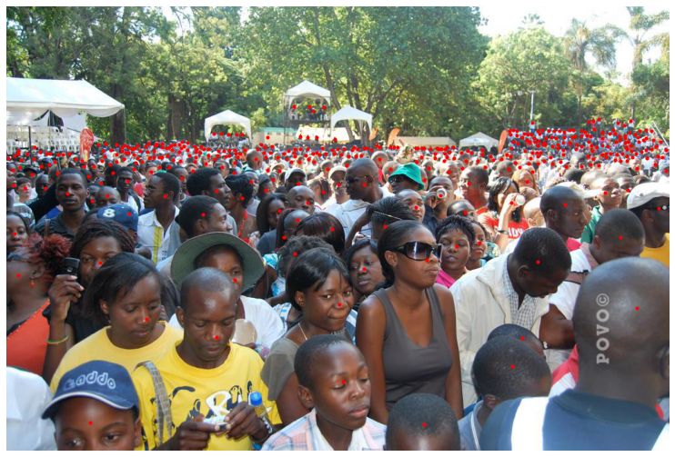
(a) A free-view image with annotations from ShanghaiTech A [19].

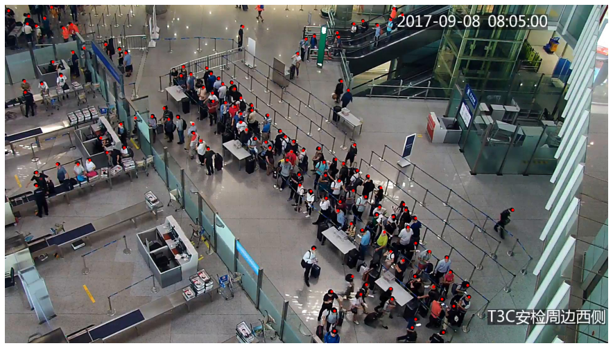
(b) A surveillance-view image with annotations from Crowd Surveillance [43].

Figure 1: Two instances of images and their corresponding dot annotations, which are usually marked at centers of people’s heads. Images from a free view can contain a much more congested crowd than those taken by surveillance cameras.

On the other hand, there are two challenges encountered during the deployment of crowd counting models. Although state-of-the-art algorithms have achieved exceptional results on several benchmark datasets, their backbones slow down the inference speed. Most use VGGs [14] as front ends, but this family of neural networks is composed of standard convolutions, indicating that hundreds of billions of arithmetic operations are required to make prediction on a $720$P image. In contrast, many $1\times 1$ and spatially separable convolutions are involved in Inception-V3 [18], significantly reducing the total amount of computation. More detailed comparison of the inference time of different CNN models can be found on Keras Applications [12]. The other difficulty is the lack of appropriately pre-trained models. The most popular benchmark datasets are UCF_CC_50 [9], ShanghaiTech (A and B) [19], and UCF-QNRF [28], so most researchers only open-source weights tuned on them to prove their models’ superiority. However, although ShanghaiTech B [19] is from a surveillance perspective, it solely represents crowded scenes, and the other three are free-view and much more congested. Hence, models trained on these datasets usually fail to generalize well to real-world data from surveillance cameras. By comparison, Crowd Surveillance [43] is another surveillance-view dataset containing both sparse and crowded scenes. This property endows models with better generalization on surveillance videos.

Hence, in this paper, inspired by Inception-V3 [18], a more diminutive crowd counting model will be proposed, and its pre-trained weights on Crowd Surveillance [43] will be open-sourced to facilitate its implementation in monitoring systems. Besides, multiple experiments will be conducted, including evaluating its performance on ShanghaiTech (A and B) [19] and Mall [6], to show that it requires fewer computation resources while preserves a high accuracy.

II Related Work

II-A The Evolvement of Crowd Counting Algorithms

Early crowd counting approaches [1, 2, 4] are based on object detection. They require laborious box annotations and are sensitive to occlusion, so later works seek to circumvent detection. Some [3, 6, 7] treat crowd counting as a regression problem and directly output the total count from a feature vector. Nevertheless, dot annotations (see Fig. 1) are underutilized in these algorithms because their loss functions are straight related to the ground-truth total count and its estimation, while the pixel-wise distribution of the crowd, which seems to be more critical, is neglected. As a result, these models suffer from poor generalization, and soon, they have been superseded by algorithms [17, 19, 27, 30, 33, 34, 35, 37, 38, 39, 40, 41, 42, 44, 45, 47, 49] that instead predict the crowd density, whose values indicate the number of people in the corresponding pixels.

However, the development of density-prediction-based approaches is not smooth; the problem of variant local scales of heads influencing a model’s performance has been haunting researchers for years. One viable solution is to leverage geometric information [17, 22] to adjust models to the scene’s geometry, but this information is usually unavailable in the test environment. Thus, other methods choose to include modules designed to cope with the variation of local scales. One of the most prominent among them is CAN [39], in which rapid scale changes are being handled by a contextual-aware module which fuses multi-scale features adaptively. Nevertheless, its backbone is still based on VGG-16 [14], resulting in extensive computation and thus improper for real-time estimation.

II-B Inception-V3

In comparison, Inception-V3 [18] is a more suitable candidate for the front end of fast algorithms since it has much fewer standard convolutions by decomposing kernels. For example, a convolutional kernel with a filter size of $3\times 3$ and $64$ output channels can be replaced with a $1\times 1$ kernel that add values along the channel, followed by a $3\times 3$ kernel to increase the number of channels. The former one performed on a $4\times 4$ image would require $13,568$ arithmetic operations, while the latter only needs $4,432$, reducing around $67\%$ computation. Large kernels ($n\times n$) can also be factorized into a $n\times 1$ kernel and a $1\times n$ kernel. Furthermore, unlike VGGs, Inceptions [15, 18, 25] have multi-column modules, so they can natively capture the scale variance. Nevertheless, it is insufficient for these modules alone to solve the problem caused by scales.

II-C The DM-Count Loss

Loss functions for training, defined on density maps, have also been well studied. Since the ground-truth density map is a sparse binary matrix, with $0$s and $1$s exceptionally unevenly distributed, functions directly based on the it are difficult to train. Thus, early methods [10, 19, 28, 39, 41] use Gaussian kernels to smooth the binary matrix, and as a result, the model’s performance is heavily affected by the quality of smoothing. However, setting suitable kernel widths is not easy because of various scales in an image. Therefore, the DM-Count loss, which uses optimal transport to measure the distance between density map distributions, has been proposed in [45] to address the challenge brought by training and Gaussian smoothing. The authors of [45] have also proved that models trained under the supervision of the DM-Count loss will have tighter upper bounds for the generalization error.

In this work, the first several blocks of Inception-V3 [18] will be used to construct the front end to speed up inference. The advantage of the context-aware module within CAN [39] will also be leveraged to adapt the model to different head scales. The inception blocks will also be exploited to reinforce the capture of contextual information. The DM-Count loss [45] will be employed in training to avoid issues caused by Gaussian smoothing.

III Inception-Based Crowd Counting

III-A Problem Formulation

Let $\bm{X}\in\bm{\mathcal{X}}\subset\mathbb{R}_{+}^{h\times w\times 3}$ be an RGB image with the height $h$ and the width $w$ and $\bm{Y}\in\bm{\mathcal{Y}}\subset\mathbb{R}_{+}^{h\times w}$ be its corresponding binary density map, i.e., for a pixel $(r,c)$, $\bm{Y}_{r,c}=1$ if and only if there is a person’s signiture (usually the head’s center) present in it. Assume $p(\bm{X})$ is the distribution of $\bm{X}$ and the dependent variable $\bm{Y}$ is always observable. For a general crowd counting algorithm and a given loss function $\mathcal{L}$ defined on $\bm{\mathcal{Y}}\times\bm{\mathcal{Y}}$, the mathematical aim is to fit a function $\bm{F}(\cdot\,;\,\bm{\omega})$ parameterized by $\bm{\omega}$ that minimizes the expected cost:

$$\int_{\bm{\mathcal{X}}}\mathcal{L}\left(\bm{F}(\bm{X};\,\bm{\omega}),\,\bm{Y}\right)\operatorname{d\!}\bm{X}.$$

Denote its minimum value as $\mathcal{C}_{\bm{F}}$, i.e.

$$\mathcal{C}_{\bm{F}}\mathrel{\mathop{\mathchar 58\relax}}=\min_{\bm{\omega}}\int_{\bm{\mathcal{X}}}\mathcal{L}\left(\bm{F}(\bm{X};\,\bm{\omega}),\,\bm{Y}\right)\operatorname{d\!}\bm{X}.$$ (1)

However, in practice, the distribution of $\bm{X}$ is unknow, and only observations of $\bm{X}$ and $\bm{Y}$ are accessible, so the problem of overfitting is inevitable. Thus, in machine learning, these data are usually split into two disjoint sets, namely, a training set $(\bm{\mathcal{X}}_{\text{tr}},\bm{\mathcal{Y}}_{\text{tr}})$ and a test set $(\bm{\mathcal{X}}_{\text{t}},\bm{\mathcal{Y}}_{\text{t}})$. The former is usually used to obtain $\hat{\bm{\omega}}$ by optmizing the training cost

$$\sum_{\bm{X}\in\bm{\mathcal{X}}_{\text{tr}}}\mathcal{L}_{\text{tr}}\left(\bm{F}(\bm{X};\,\bm{\omega}),\,\bm{Y}\right),$$

while the latter is used to estimate $\mathcal{C}_{\bm{F}}$ by calculating

$$\tilde{\mathcal{C}}_{\bm{F}}\mathrel{\mathop{\mathchar 58\relax}}=\sum_{\bm{X}\in\bm{\mathcal{X}}_{\text{t}}}\mathcal{L}\left(\bm{F}(\bm{X};\,\hat{\bm{\omega}}),\,\bm{Y}\right).$$

Since this paper is interested in real-time estimation, the form of $\bm{F}$ is constrained within a particular range $\bm{\mathcal{F}}$. The prediction must also remain as precise as possible, so ideally, the ultimate purpose is to solve

$$\min_{\bm{F}\in\bm{\mathcal{F}}}\tilde{C}_{\bm{F}}.$$ (2)

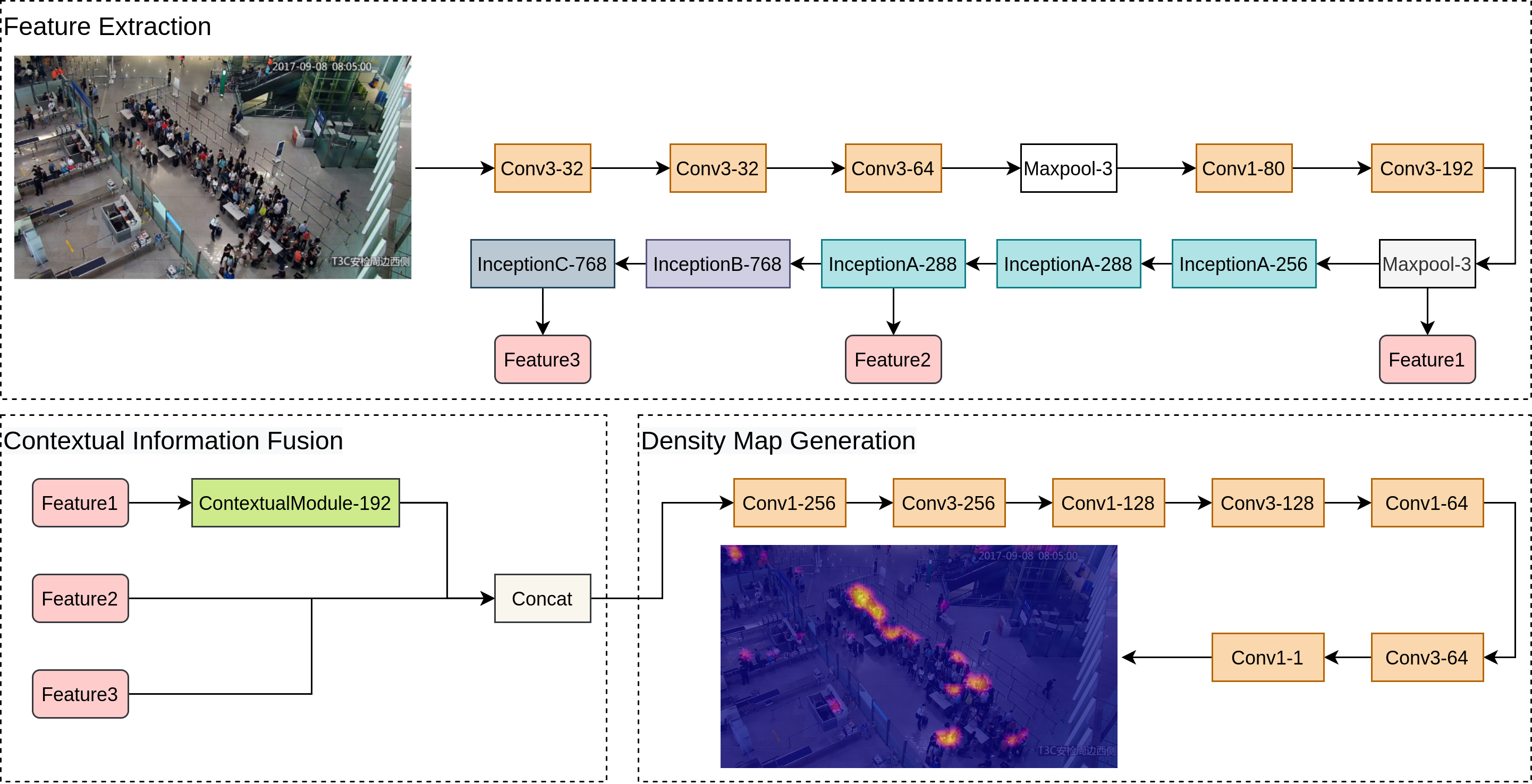
Figure 2: The architecture of the proposed model. It uses the first twelve layers of Inception-V3 [18] to obtain features at different levels from the input image. The contextual module from CAN [39] will be leverage to process Feature1. Then they are fused and passed into the decoder to generate the predicted density map.

III-B Model Architecture

Due to the unfeasibility to solve (2), and considering the benefits of those models mentioned in Section II, this paper comes up with a suboptimal solution instead. Its structure is shown in Fig. 2.

III-B1 The Encoding Front End

The starting point is a network consisting of the first 12 blocks of a pre-trained Inception-V3 [18]. Feature1, which is the output from the second max-pooling layer, is analogous to the base features extracted by the VGG component in CAN [39]. The difference is that Feature1 comes from a much shallower layer, accommodating more rich details. As the it goes deeper, the output from the third Inception-A block [18] is cloned as Feature2. To avoid introducing too many parameters, the original Inception-V3 [18] is truncated after the first Inception-C block [18], whose output is denoted as Feature3.

III-B2 Contextual Information Extraction

There are two different approaches used to extract contextual information. One is to impose the contextual module from [39], in which filters with different sizes (1, 2, 3 and 6) are employed, on Feature1 to produce scale-aware features. As the $1\times 1$ kernel is utilized, abundant details can be well preserved. These processed features are also context-aware, contributing remarkably to accurate predictions of heads at both small and large scales. The other avenue is to utilize the Inception blocks [18] within the front end. These blocks also have bottleneck structures to learn both sparse and non-sparse features, and the dissimilarity is that they are much deeper and during the extraction of Feature2 and Feature3, contextual information is repeatedly fused. As Feature2 and Feature3 already contains contextual information, there is no further processing of them, and all these context-aware features are finally combined along the channel. Exploiting disparate strategies can reinforce the model’s robustness.

III-B3 The Decoding Back End

The concatenated features are being input into this component to generate the predicted density map. $1\times 1$ convolutions are executed before standard convolutions to decrease the number of channels, so the overall computation can be notably reduced. Finally, tensor values are summed up across the channel to generate the predicted density map. Note that since downsampling operations like pooling with the stride of 2 are used, the size of the predicted density map is 8 times smaller. To recover it to the full size, upsampling such as interpolation can be leveraged.

III-C Training Details

III-C1 Pre-Processing

As for pre-processing, because of the reduced output size, the ground-truth density map needs to be downsampled to have the same shape. Besides, since widths and heights of images usually differ within any dataset, cropping is utilized so that data can be batched in training.

III-C2 Loss Functions

For the processed ground truth $\bm{Y}$ and its approximation $\hat{\bm{Y}}$, the loss function for training is the DM-Count loss defined in [45], which comprises the counting loss $\ell_{\text{C}}$, the optimal transport loss $\ell_{\text{OT}}$ and the total variation loss $\ell_{\text{TV}}$.

As the optimal transport measures the dissimilarity between two probability distributions, vectorizing $\bm{Y}$ and $\hat{\bm{Y}}$ brings easier definitions. Denote the downsampled width and height as $w^{\prime}$ and $h^{\prime}$. Let $\bm{y}$ and $\hat{\bm{y}}$ be the unrolled forms of $\bm{Y}$ and $\hat{\bm{Y}}$, so $\bm{y},\,\hat{\bm{y}}\in\mathbb{R}^{h^{\prime}\times w^{\prime}}$. Since each element of $\bm{y}$ (or $\hat{\bm{y}}$) represents the corresponding crowd density at that pixel, the total count is exactly its $L_{1}$ norm. Thus, the counting loss is defined as

$$\ell_{\text{C}}(\bm{y},\,\hat{\bm{y}})\mathrel{\mathop{\mathchar 58\relax}}=\left|\|\bm{y}\|_{1}-\|\hat{\bm{y}}\|_{1}\right|,$$ (3)

which measures the difference of the ground-truth and predicted counts.

Similar to the Kullback-Leibler divergence and the Jensen-Shannon divergece, Monge-Kantorovich’s optimal transport cost is another way to measure the distance between two probability distributions, but it has certain better optimization properties [20] and therefore is exploited. Assume $\bm{p}$ and $\bm{q}$ are two probability masses, i.e., $\bm{p}_{i},\,\bm{q}_{i}\geq 0$ and $\sum_{i=1}^{n}\bm{p}_{i}=\sum_{j=1}^{n}\bm{q}_{j}=1$. Let $c(\bm{p}_{i},\,\bm{q}_{j})$ be the cost of transforming $\bm{p}_{i}$ to $\bm{q}_{j}$ and $\bm{C}\in\mathbb{R}_{+}^{n\times n}$ such that $\bm{C}_{i,j}=c(\bm{p}_{i},\,\bm{q}_{j})$. Then the optimal transport cost $\mathcal{W}(\bm{p},\,\bm{q})$ is defined as the minimum cost of transforming $\bm{p}$ into $\bm{q}$, which is

$$\mathcal{W}(\bm{p},\,\bm{q})\mathrel{\mathop{\mathchar 58\relax}}=\min_{\bm{\pi}\in\mathbb{R}^{n\times n}_{+}}\langle\bm{\pi},\,\bm{C}\rangle.$$ (4)

For $\bm{\pi}\in\mathbb{R}^{n\times n}_{+}$ to be a valid transformation, it needs to satisfy $\sum_{k=1}^{n}\bm{\pi}_{i,k}=\bm{p}_{i}$ and $\sum_{k=1}^{n}\bm{\pi}_{k,j}=\bm{q}_{j}$, $\forall i,j\in\mathbb{N}_{+}$, $1\leq i,\,j\leq n$.

Hence, in [45], by viewing $\bm{y}$ and $\hat{\bm{y}}$ as two unnormalized distributions, the optimal transport loss is defined as

$$\ell_{\text{OT}}(\bm{y},\,\hat{\bm{y}})\mathrel{\mathop{\mathchar 58\relax}}=\mathcal{W}\left(\frac{\bm{y}}{\|\bm{y}\|_{1}},\,\frac{\hat{\bm{y}}}{\|\hat{\bm{y}}\|_{1}}\right),$$ (5)

in which the transport cost function is defined as the squared Euclidean distance of corresponding pixels. For example, suppose $\bm{y}_{h}$ corresponds to pixel $(i,\,j)$ in $\bm{Y}$ and $\hat{\bm{y}}_{k}$ corresponds to pixel $(p,\,q)$ in $\hat{\bm{Y}}$, then

$$c\left(\frac{\bm{y}_{h}}{\|\bm{y}\|_{1}},\,\frac{\hat{\bm{y}}_{k}}{\|\hat{\bm{y}}\|_{1}}\right)\mathrel{\mathop{\mathchar 58\relax}}=(p-i)^{2}+(q-j)^{2}.$$ (6)

Notice that the definition of (4) involves an optimization problem. Different from [45], in this paper, it is solved by the Sinkhorn-Knopp matrix scaling algorithm proposed in [8] and implemented by POT [46]. Since numerical errors will also be introduced in this process, the total variation loss defined in [45] is still included to stablize training:

$$\ell_{\text{TV}}(\bm{y},\,\hat{\bm{y}})\mathrel{\mathop{\mathchar 58\relax}}=\frac{1}{2}\left\|\frac{\bm{y}}{\|\bm{y}\|_{1}}-\frac{\hat{\bm{y}}}{\|\hat{\bm{y}}\|_{1}}\right\|_{1}.$$ (7)

The overall loss function [45] is defined as

$$\ell(\bm{y},\,\hat{\bm{y}})\mathrel{\mathop{\mathchar 58\relax}}=\ell_{\text{C}}(\bm{y},\,\hat{\bm{y}})+\lambda_{1}\ell_{\text{OT}}(\bm{y},\,\hat{\bm{y}})+\lambda_{2}\|\bm{y}\|_{1}\ell_{\text{TV}}(\bm{y},\,\hat{\bm{y}}),$$ (8)

in which $\lambda_{1}$ and $\lambda_{2}$ are tunable hyper-parameters.

III-C3 Optimization

AdamW [32] with exponential learning rate decay is used as the optmizer, and the initial learning rate used on all datasets is $10^{-4}$. The model’s performance on validation sets is evaluated after each epoch to avoid overfitting to training sets.

IV Experiments

In this section, the proposed model (ICC) will be evaluated, so evaluation metrics and benchmark datasets will be first introduced. Then it will be compared with the state-of-the-art approaches, and finally, an ablation study about the two avenues to extract contextual information will be conducted.

IV-A Evaluation Metrics

Following previous works [19, 21, 24, 29, 39, 45, 48, 49], the mean absolute error (MAE) and the root mean squared error (RMSE) are utilized as two evaluation metrics. For a set of ground-truth counts $\{{z}_{1},\,\cdots,\,{z}_{N}\}$ and their predictions $\{\hat{{z}}_{1},\cdots,\,\hat{{z}}_{N}\}$, these two metrics are defined as

$$\text{MAE}\mathrel{\mathop{\mathchar 58\relax}}=\frac{1}{N}\sum_{i=1}^{N}|z_{i}-\hat{z}_{i}|,$$ (9)

and

$$\text{RMSE}\mathrel{\mathop{\mathchar 58\relax}}=\sqrt{\frac{1}{N}\sum_{i=1}^{N}(z_{i}-\hat{z}_{i})^{2}}.$$ (10)

The number of floating-point operations required to infer on a $1080$P ($1080\times 1920$) image is leveraged to quantify the each model’s computational complexity.

IV-B Benchmark Datasets

Three datasets, ShanghaiTech A [19], ShanghaiTech B [19] and Mall [6] are used for comparison, although there are some other classic benchmark datasets in crowd counting, such as UCF_CC_50 [10] and UCF-QNRF [28]. This is because the primary purpose of this paper is to provide an efficient model for surveillance systems, only one free-view dataset (which is ShanghaiTech A [19]) is needed to reflect the model’s general crowd counting capability. The Crowd Surveillance dataset [43] will also be introduced, as the power of weights trained on it is demonstrated in Section IV-C.

IV-B1 ShanghaiTech A [19]

It is composed of $482$ images with annotations, $300$ for training and $182$ for testing. The average resolution of these images is $589\times 868$, and the average number of individuals present in one is approximately $501$. These images are not guaranteed to be from surveillance cameras, so this dataset is only used to prove the model’s ability to count crowds in free-view images. The orignal training set is split into a new training set ($80\%$) and a validation set ($20\%$). The latter is designated to tune hyper-paramters, such as the number of epochs for training. Fig. 3 provides visualization of the proposed model’s predictions on two randomly selected test images from ShanghaiTech A [19].

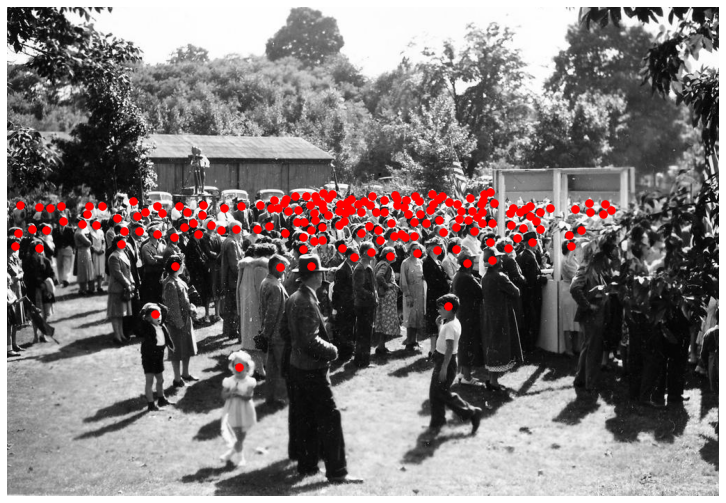
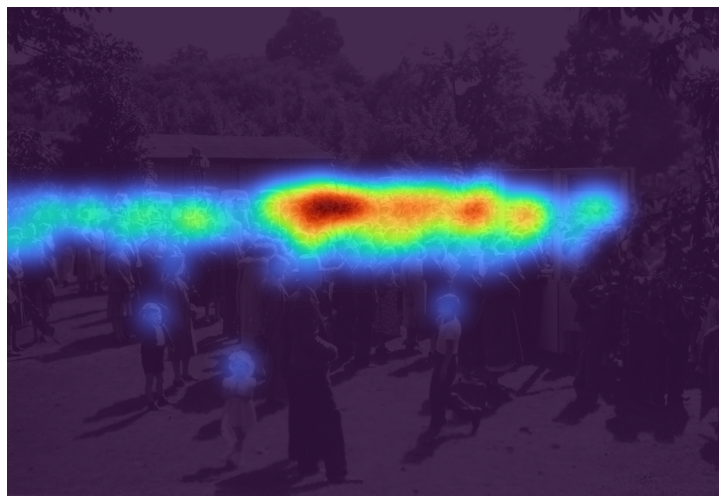
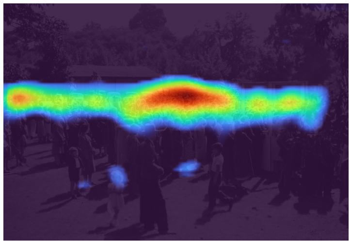
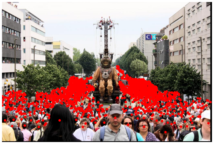
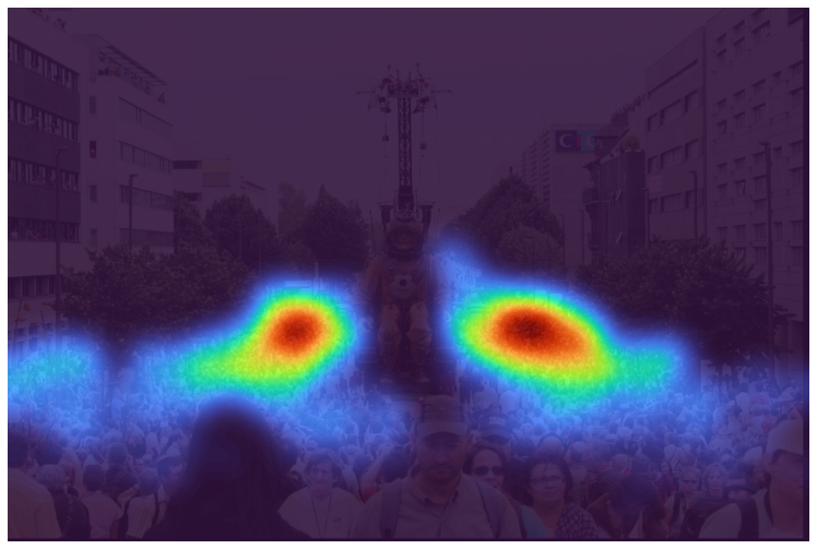
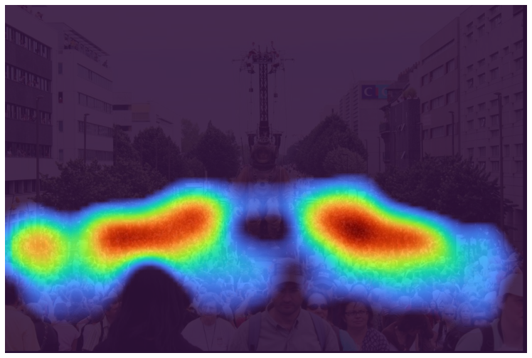
Figure 3: Crowd density estimation on two images from ShanghaiTech A [19]. 3 and 3 are images annotated with original ground truths, whose corresponding Gaussian smoothed (with $\sigma=20$) alternates are shown in 3 and 3. The proposed algorithm’s predictions are visualized in 3 and 3, which demonstrate its good performance on unseen data.

IV-B2 ShanghaiTech B [19]

This dataset comprehends $400$ images for training and $316$ for testing. These images come from surveillance cameras in different scenes. The average resolution is $768\times 1024$ and the mean count is about $123$, which indicates that crowds in these images are densely distributed. The same data splitting strategy is exploited to generate a validation dataset, and the proposed approach’s good generalization is illustrated in Fig. 4.

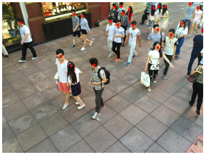
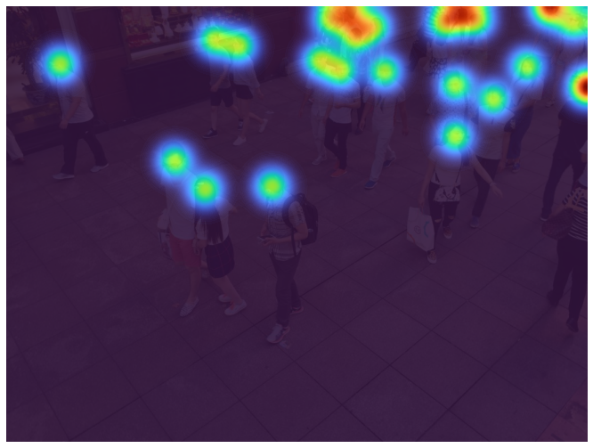
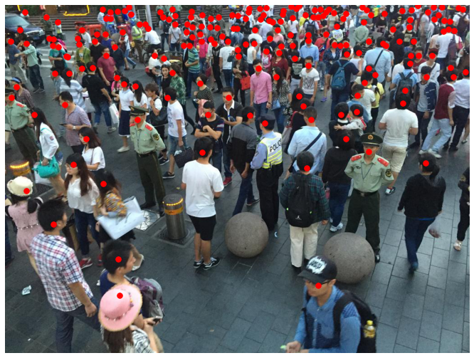
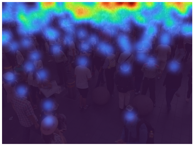
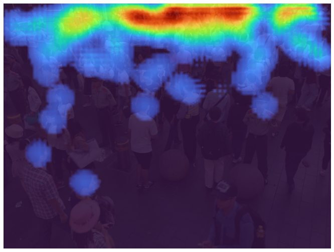
Figure 4: 4 and 4 are two test images from ShanghaiTech B [19], annotated with original ground truths. The Gaussian kernel with $\sigma=20$ is adopted in smoothing to produce 4 and 4, and 4 and 4 are plots of the corresponding predictions.

IV-B3 Mall [6]

Although it is also surveillance-view, its difference from ShanghaiTech B [19] is that its images are frames of a surveillance video, whose source is a fixed camera at a shopping center. These images are all $480\times 640$ with the mean count of $31$. Since the principal goal of the proposed method is to become applicable in surveillance systems, this dataset is the most ideal one for evaluation. Following previous works [6, 26, 30, 31, 36, 50], the training set comprises the first $800$ frames, and test set is composed of the rest. Results of predictions of two test images are shown in Fig. 5.

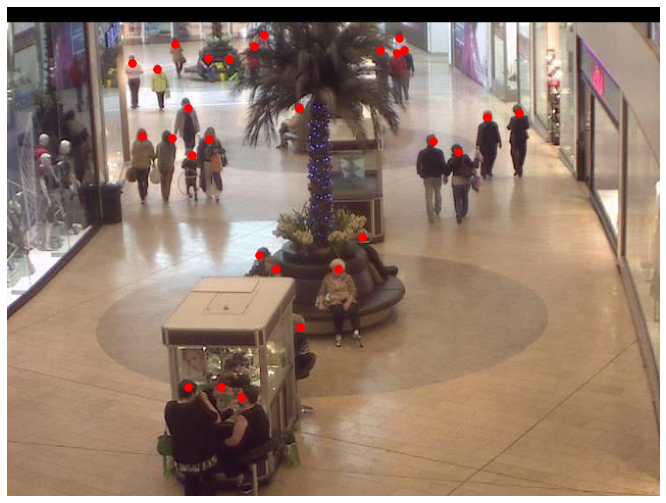
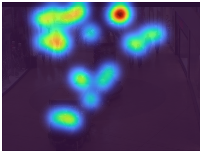
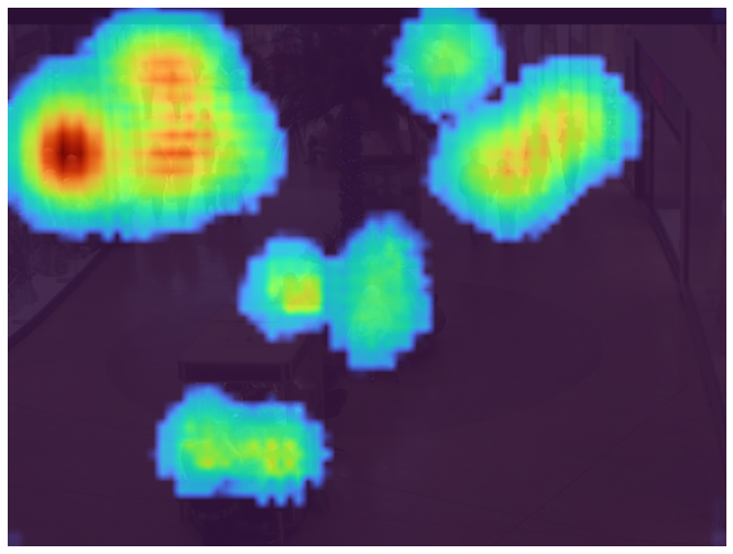
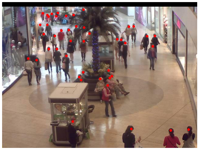
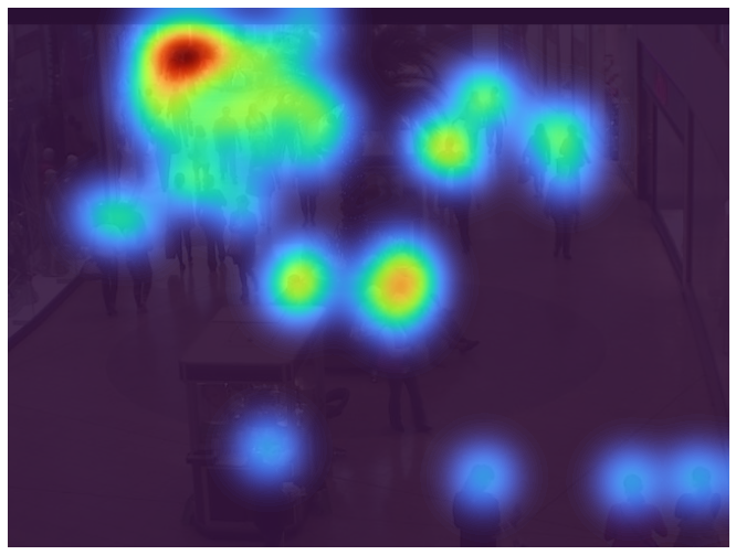
Figure 5: Crowd density predictions of two test images from Mall [6].

IV-B4 Crowd Surveillance [43]

It is one of the largest published crowd counting datasets that are from surveillance viewpoints: $10,880$ images constitute the training set, and $3,065$ account for the test set. More crucially, these images are from numerous free scenes instead of those fixed, and the total count spans a large range, so models trained on it can be exposed to more various situations and thus become more robust. Fig. 6 shows comparison of the distribution of total counts of Crowd Surveillance [43] against those of ShanghaiTech (A and B) [19].

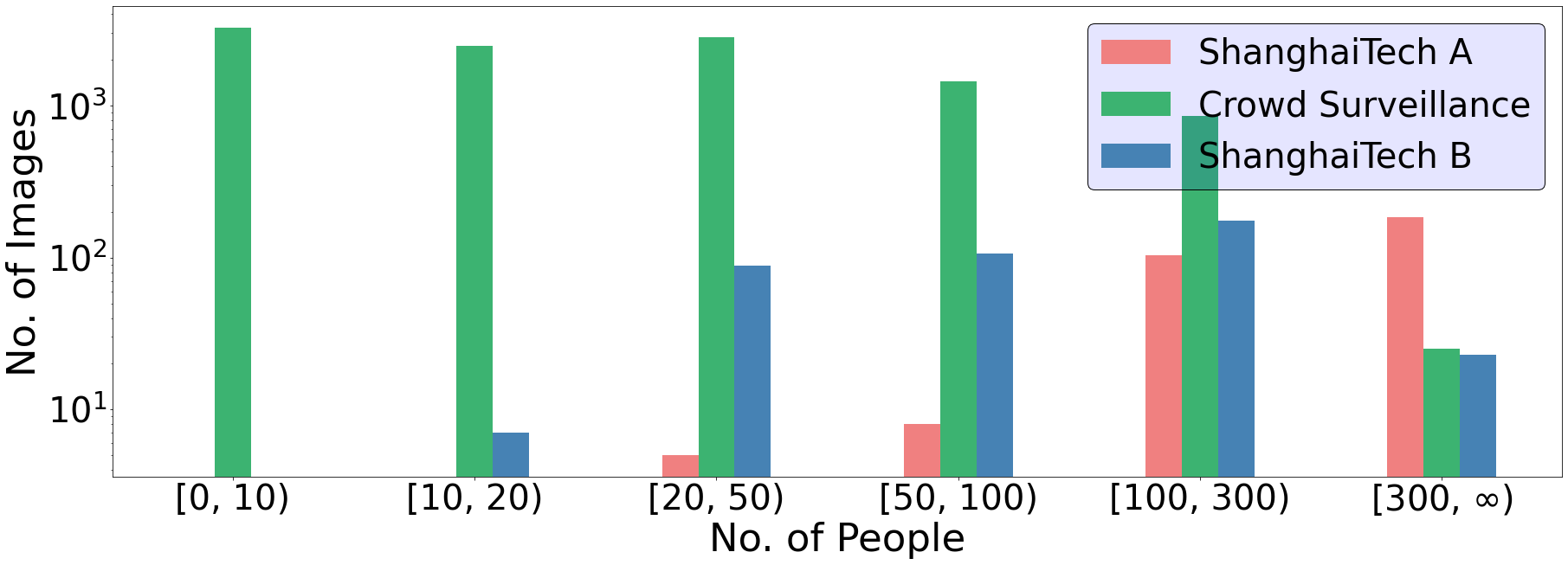
Figure 6: A histogram of total counts from the training sets. As it presents, the total counts of crowds in Crowd Surveillance is more uniformly distributed, so models trained on it should possess excellent generalization on others.

In practice, $20\%$ training data are dedicated to validation, and similar visualization of predictions is provided in Fig. 7.

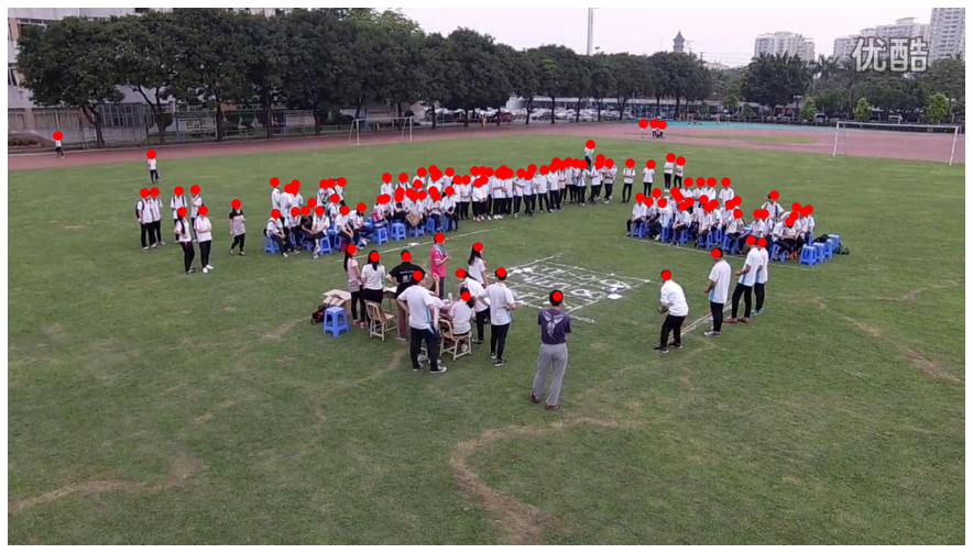
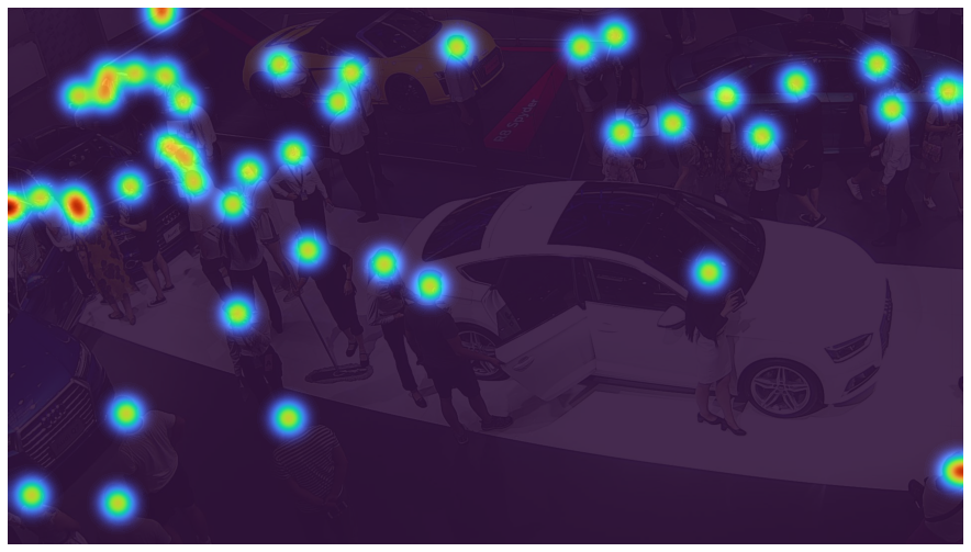
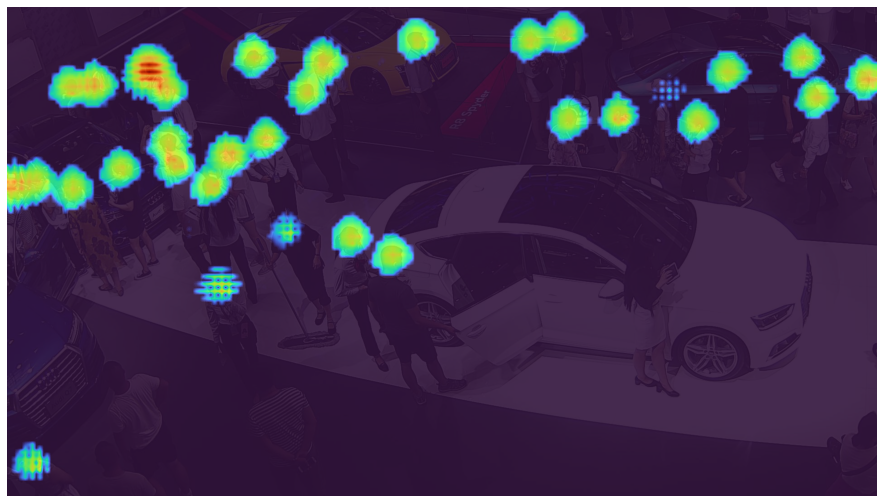
Figure 7: Crowd density predictions of two test images from Crowd Surveillance [43]. The proposed model has accomplished fine results on this dataset, with the test MAE being $4.01$.

IV-C Model Comparison

In this section, the performance of the proposed model on ShanghaiTech datasets [19] is compared only with open-source state-of-the-art algirithms, since the computational complexity needs to be measured. Regarding Mall [6], as many approaches that have published results on this dataset have not open-sourced their code, this quantity will not be computed. A randomly generated $1080\times 1920$ image is used to calculate the number of arithmetic operations.

TABLE I: Comparison with state-of-the-art models on ShanghaiTech [19]

Methods	Complexitya	Part A		Part B
		MAE	RMSE	MAE	RMSE
MCNN [19]	56.21 G	110.2	173.2	26.4	41.3
CMTL [24]	243.80 G	101.3	152.4	20.0	31.1
CSRNet [29]	857.84 G	68.2	115.0	10.6	16.0
CAN [39]	908.05 G	62.3	100.0	7.8	12.2
DM-Count [45]	853.70 G	59.7	95.7	7.4	11.8
M-SegNet [48]	749.73 G	60.55	100.8	6.8	10.4
SASNet [47]	1.84 T	54.59	88.38	6.35	9.9
ICC (proposed)	125.53 G	76.97	130.16	8.46	15.20
$\mathrm{a}$. The computational complexity of each model is quantified by the
number of arithmetic operations needed to make inference on a $1080$P
image.

TABLE II: Comparison with advanced algorithms on Mall [6]

Methods	MAE	RMSE
Chen et al. [6]	3.15	15.7
ConvLSTM [26]	2.24	8.50
DecideNet [30]	1.52	1.90
DRSAN [31]	1.72	2.10
SAAN [36]	1.28	1.68
LA-Batch [50]	1.34	1.90
ICC (proposed)	2.16	2.74
ICC (proposed) + Crowd Surveillance [43]	3.79	4.77

Results are summerized in Table I and II, showing that the proposed model have comparatively good performances on these three datasets. Compared with the top algorithm SASNet [47], the computation can be reduced by $93.18\%$ by sacrificing $41.00\%$, $47.27\%$, $33.23\%$ and $53.54$ performance, under the metrics of MAE and MSE on ShanghaiTech A and B [19], respectively. As for its comparison against the second best models (DM-Count [45] and M-SegNet [48] on ShanghaiTech A and B [19] respectively), losses have to increase by $28.93\%$, $36.00\%$, $24.41\%$ and $46.15\%$, in exchange for $85.30\%$ and $83.26\%$ decrease in calculations. More remarkably, on ShanghaiTech B [19], which is more similar to the deployment environment, the proposed architecture outperforms CSRNet [29] under both metrics, with $85.3\%$ operations less, demonstrating its exceedingly high efficiency.

As for the Mall [6] dataset, the proposed method also achieves comparable results on it. Table II shows that leading models can control both MSE and RMSE less than $3.0$, and the proposed can also manage to do so. Also, for an ICC that has no access to the training data of Mall [6] (denoted as “ICC (proposed) + Crowd Surveillance [43]” in Table II), exploiting trained weights on Crowd Surveillance [43] is effective, since its tset RMSE is $4.77$, much less than those of Chen et al. [6] and ConvLSTM [26], and the gap between MAEs of the two ICCs is not immense. This benefit can contribute vastly to the deployment of crowd counting methods. However, because the authors of those approaches listed in Table II have not open sourced their code for implementation yet, each model’s computational complexity is not compared.

IV-D Ablation Study

In this section, the effectiveness of the context-aware module [39] and those inception blocks [18] is researched by evaluating the performance of ICC without these modules on ShanghaiTech B [19]. Except for the structure, everything else in the setting remains the same. Results are shown in Table III, showing that including both the contextual module from CAN [39] and inception blocks [18] can both significantly lower the errors. However, as the difference between the model’s performance with and without the contextual module is notably prominent, the contextual module has the major role to take in the extraction of contextual information, and as claimed in previous sections, the function of inception blocks [18] is to reinforce this process.

TABLE III: Component Analysis of ICC on ShanghaiTech B [19]

Methods	MAE	RMSE
Original	8.46	15.20
No Contextual Module	25.56	44.72
No Inception Blocks	10.62	17.83

V Conclusion

In this paper, a convolutional neural network, established on Inception-V3 [18] and CAN [39] has been proposed to facilitate the deployment of crowd counting models in surveillance systems. The proposed method is much less computationally complex compared with the state-of-the-art algorithms, while its performance is not significantly harmed. This property has been testified by various experiments on benchmark datasets. Both context-aware components within the model have been proved to be useful, and this work also shows models pre-trained on Crowd Surveillance [43] have good generalization.

References

- [1] Sheng-Fuu Lin, Jaw-Yeh Chen and Hung-Xin Chao “Estimation of number of people in crowded scenes using perspective transformation” In IEEE Transactions on Systems, Man, and Cybernetics - Part A: Systems and Humans 31.6, 2001, pp. 645–654 DOI: 10.1109/3468.983420
- [2] Min Li, Zhaoxiang Zhang, Kaiqi Huang and Tieniu Tan “Estimating the number of people in crowded scenes by MID based foreground segmentation and head-shoulder detection” In 2008 19th International Conference on Pattern Recognition, 2008, pp. 1–4 DOI: 10.1109/ICPR.2008.4761705
- [3] Antoni B. Chan and Nuno Vasconcelos “Bayesian Poisson regression for crowd counting” In 2009 IEEE 12th International Conference on Computer Vision, 2009, pp. 545–551 DOI: 10.1109/ICCV.2009.5459191
- [4] Weina Ge and Robert T. Collins “Marked point processes for crowd counting” In 2009 IEEE Conference on Computer Vision and Pattern Recognition, 2009, pp. 2913–2920 DOI: 10.1109/CVPR.2009.5206621
- [5] Victor Lempitsky and Andrew Zisserman “Learning To Count Objects in Images” In Advances in Neural Information Processing Systems 23 Curran Associates, Inc., 2010 URL: https://proceedings.neurips.cc/paper/2010/file/fe73f687e5bc5280214e0486b273a5f9-Paper.pdf
- [6] Ke Chen, Chen Change Loy, Shaogang Gong and Tony Xiang “Feature Mining for Localised Crowd Counting” In British Machine Vision Conference, BMVC 2012, Surrey, UK, September 3-7, 2012 BMVA Press, 2012, pp. 1–11 DOI: 10.5244/C.26.21
- [7] Ke Chen, Shaogang Gong, Tao Xiang and Chen Change Loy “Cumulative Attribute Space for Age and Crowd Density Estimation” In 2013 IEEE Conference on Computer Vision and Pattern Recognition, 2013, pp. 2467–2474 DOI: 10.1109/CVPR.2013.319
- [8] Marco Cuturi “Sinkhorn distances: Lightspeed computation of optimal transport” In Advances in neural information processing systems 26, 2013, pp. 2292–2300
- [9] Haroon Idrees, Imran Saleemi, Cody Seibert and Mubarak Shah “Multi-source Multi-scale Counting in Extremely Dense Crowd Images” In 2013 IEEE Conference on Computer Vision and Pattern Recognition, 2013, pp. 2547–2554 DOI: 10.1109/CVPR.2013.329
- [10] Haroon Idrees, Imran Saleemi, Cody Seibert and Mubarak Shah “Multi-source multi-scale counting in extremely dense crowd images” In Proceedings of the IEEE conference on computer vision and pattern recognition, 2013, pp. 2547–2554
- [11] Thomas Moranduzzo and Farid Melgani “Automatic Car Counting Method for Unmanned Aerial Vehicle Images” In IEEE Transactions on Geoscience and Remote Sensing 52.3, 2014, pp. 1635–1647 DOI: 10.1109/TGRS.2013.2253108
- [12] François Chollet “Keras”, https://keras.io, 2015
- [13] Mingpei Liang et al. “Counting and Classification of Highway Vehicles by Regression Analysis” In IEEE Transactions on Intelligent Transportation Systems 16.5, 2015, pp. 2878–2888 DOI: 10.1109/TITS.2015.2424917
- [14] Karen Simonyan and Andrew Zisserman “Very Deep Convolutional Networks for Large-Scale Image Recognition” In International Conference on Learning Representations, 2015
- [15] Christian Szegedy et al. “Going deeper with convolutions” In Proceedings of the IEEE conference on computer vision and pattern recognition, 2015, pp. 1–9
- [16] Evgeny Toropov et al. “Traffic flow from a low frame rate city camera” In 2015 IEEE International Conference on Image Processing (ICIP), 2015, pp. 3802–3806 DOI: 10.1109/ICIP.2015.7351516
- [17] Cong Zhang, Hongsheng Li, Xiaogang Wang and Xiaokang Yang “Cross-scene crowd counting via deep convolutional neural networks” In Proceedings of the IEEE conference on computer vision and pattern recognition, 2015, pp. 833–841
- [18] Christian Szegedy et al. “Rethinking the inception architecture for computer vision” In Proceedings of the IEEE conference on computer vision and pattern recognition, 2016, pp. 2818–2826
- [19] Yingying Zhang et al. “Single-image crowd counting via multi-column convolutional neural network” In Proceedings of the IEEE conference on computer vision and pattern recognition, 2016, pp. 589–597
- [20] Martin Arjovsky, Soumith Chintala and Léon Bottou “Wasserstein generative adversarial networks” In International conference on machine learning, 2017, pp. 214–223 PMLR
- [21] Deepak Babu Sam, Shiv Surya and R Venkatesh Babu “Switching convolutional neural network for crowd counting” In Proceedings of the IEEE conference on computer vision and pattern recognition, 2017, pp. 5744–5752
- [22] Di Kang, Debarun Dhar and Antoni B Chan “Incorporating side information by adaptive convolution” In Proceedings of the 31st International Conference on Neural Information Processing Systems, 2017, pp. 3870–3880
- [23] Hao Lu et al. “TasselNet: counting maize tassels in the wild via local counts regression network” In Plant methods 13.1 BioMed Central, 2017, pp. 1–17
- [24] Vishwanath A Sindagi and Vishal M Patel “Cnn-based cascaded multi-task learning of high-level prior and density estimation for crowd counting” In 2017 14th IEEE International Conference on Advanced Video and Signal Based Surveillance (AVSS), 2017, pp. 1–6 IEEE
- [25] Christian Szegedy, Sergey Ioffe, Vincent Vanhoucke and Alexander A Alemi “Inception-v4, inception-resnet and the impact of residual connections on learning” In Thirty-first AAAI conference on artificial intelligence, 2017
- [26] Feng Xiong, Xingjian Shi and Dit-Yan Yeung “Spatiotemporal modeling for crowd counting in videos” In Proceedings of the IEEE International Conference on Computer Vision, 2017, pp. 5151–5159
- [27] Xinkun Cao, Zhipeng Wang, Yanyun Zhao and Fei Su “Scale aggregation network for accurate and efficient crowd counting” In Proceedings of the European Conference on Computer Vision (ECCV), 2018, pp. 734–750
- [28] Haroon Idrees et al. “Composition loss for counting, density map estimation and localization in dense crowds” In Proceedings of the European Conference on Computer Vision (ECCV), 2018, pp. 532–546
- [29] Yuhong Li, Xiaofan Zhang and Deming Chen “Csrnet: Dilated convolutional neural networks for understanding the highly congested scenes” In Proceedings of the IEEE conference on computer vision and pattern recognition, 2018, pp. 1091–1100
- [30] Jiang Liu, Chenqiang Gao, Deyu Meng and Alexander G Hauptmann “Decidenet: Counting varying density crowds through attention guided detection and density estimation” In Proceedings of the IEEE Conference on Computer Vision and Pattern Recognition, 2018, pp. 5197–5206
- [31] Lingbo Liu et al. “Crowd counting using deep recurrent spatial-aware network” In Proceedings of the 27th International Joint Conference on Artificial Intelligence, 2018, pp. 849–855
- [32] Ilya Loshchilov and Frank Hutter “Decoupled Weight Decay Regularization” In International Conference on Learning Representations, 2018
- [33] Erika Lu, Weidi Xie and Andrew Zisserman “Class-agnostic counting” In Asian conference on computer vision, 2018, pp. 669–684 Springer
- [34] Viresh Ranjan, Hieu Le and Minh Hoai “Iterative crowd counting” In Proceedings of the European Conference on Computer Vision (ECCV), 2018, pp. 270–285
- [35] Deepak Babu Sam, Neeraj N Sajjan, R Venkatesh Babu and Mukundhan Srinivasan “Divide and grow: Capturing huge diversity in crowd images with incrementally growing cnn” In Proceedings of the IEEE conference on computer vision and pattern recognition, 2018, pp. 3618–3626
- [36] Mohammad Hossain, Mehrdad Hosseinzadeh, Omit Chanda and Yang Wang “Crowd counting using scale-aware attention networks” In 2019 IEEE Winter Conference on Applications of Computer Vision (WACV), 2019, pp. 1280–1288 IEEE
- [37] Chenchen Liu, Xinyu Weng and Yadong Mu “Recurrent attentive zooming for joint crowd counting and precise localization” In Proceedings of the IEEE/CVF Conference on Computer Vision and Pattern Recognition, 2019, pp. 1217–1226
- [38] Ning Liu et al. “Adcrowdnet: An attention-injective deformable convolutional network for crowd understanding” In Proceedings of the IEEE/CVF Conference on Computer Vision and Pattern Recognition, 2019, pp. 3225–3234
- [39] Weizhe Liu, Mathieu Salzmann and Pascal Fua “Context-aware crowd counting” In Proceedings of the IEEE/CVF Conference on Computer Vision and Pattern Recognition, 2019, pp. 5099–5108
- [40] Miaojing Shi, Zhaohui Yang, Chao Xu and Qijun Chen “Revisiting perspective information for efficient crowd counting” In Proceedings of the IEEE/CVF Conference on Computer Vision and Pattern Recognition, 2019, pp. 7279–7288
- [41] Jia Wan and Antoni Chan “Adaptive density map generation for crowd counting” In Proceedings of the IEEE/CVF International Conference on Computer Vision, 2019, pp. 1130–1139
- [42] Haipeng Xiong et al. “From open set to closed set: Counting objects by spatial divide-and-conquer” In Proceedings of the IEEE/CVF International Conference on Computer Vision, 2019, pp. 8362–8371
- [43] Zhaoyi Yan et al. “Perspective-guided convolution networks for crowd counting” In Proceedings of the IEEE/CVF International Conference on Computer Vision, 2019, pp. 952–961
- [44] Anran Zhang et al. “Relational attention network for crowd counting” In Proceedings of the IEEE/CVF International Conference on Computer Vision, 2019, pp. 6788–6797
- [45] Boyu Wang, Huidong Liu, Dimitris Samaras and Minh Hoai Nguyen “Distribution Matching for Crowd Counting” In Advances in Neural Information Processing Systems 33, 2020
- [46] Rémi Flamary et al. “POT: Python Optimal Transport” In Journal of Machine Learning Research 22.78, 2021, pp. 1–8 URL: http://jmlr.org/papers/v22/20-451.html
- [47] Qingyu Song et al. “To Choose or to Fuse? Scale Selection for Crowd Counting” In Proceedings of the AAAI Conference on Artificial Intelligence 35.3, 2021, pp. 2576–2583
- [48] Pongpisit Thanasutives, Ken-ichi Fukui, Masayuki Numao and Boonserm Kijsirikul “Encoder-Decoder Based Convolutional Neural Networks with Multi-Scale-Aware Modules for Crowd Counting” In 2020 25th International Conference on Pattern Recognition (ICPR), 2021, pp. 2382–2389 IEEE
- [49] Jia Wan, Ziquan Liu and Antoni B Chan “A Generalized Loss Function for Crowd Counting and Localization” In Proceedings of the IEEE/CVF Conference on Computer Vision and Pattern Recognition, 2021, pp. 1974–1983
- [50] Joey Tianyi Zhou et al. “Locality-Aware Crowd Counting” In IEEE Transactions on Pattern Analysis and Machine Intelligence IEEE, 2021