Policy Gradient Methods for Designing Dynamic Output Feedback Controllers
Abstract
This paper proposes model-based and model-free policy gradient methods (PGMs) for designing dynamic output feedback controllers for discrete-time partially observable systems. To fulfill this objective, we first show that any dynamic output feedback controller design is equivalent to a state-feedback controller design for a newly introduced system whose internal state is a finite-length input-output history (IOH). Next, based on this equivalency, we propose a model-based PGM and show its global linear convergence by proving that the Polyak-Lojasiewicz inequality holds for a reachability-based lossless projection of the IOH dynamics. Moreover, we propose two model-free implementations of the PGM: the multi- and single-episodic PGM. The former is a Monte Carlo approximation of the model-based PGM, whereas the latter is a simplified version of the former for ease of use in real systems. A sample complexity analysis of both methods is also presented. Finally, the effectiveness of the model-based/model-free PGMs is investigated through a numerical simulation.
Index Terms:
Partially observable systems, dynamic output feedback control, policy gradient method, non-convex optimization, data-driven control, sample complexity analysisI Introduction
Data-driven control methodologies are classified into two categories: direct approaches [1, 2, 3, 4], which design controllers directly from data, and indirect approaches [5, 6, 7], which identify the target system from the data and then apply conventional model-based control methods. Recent work has shown that the amounts of data required for each approach are equal when optimizing control performance for discrete-time linear systems [8]. This motivates us to determine whether other differences exist between the two approaches aside from the total amounts of data.
One difference would be the control performance achieved when using a limited amount of data, that is, less than the abovementioned required amount. Though indirect approaches can find a gray model from such limited data [9], the controller designed via the identified gray model may not improve the control performance, owing to model uncertainties. In contrast, direct approaches, especially for online learning methods that gradually improve controllers while collecting data, are potentially continuous with respect to the data amount and control performance.
Online learning methods can be divided into two categories: methods that update the value/Q functions [10] and methods that update the policy directly [11, 12, 13, 14, 15]. Though the former can handle general control policies, the convergence speed is usually slower than that of the latter owing to its generality. The most well-known latter approach is the policy gradient method (PGM) [10, 16]. However, the convergence of the control policy to an optimal one is not guaranteed in general. Recently, the paper [11] has shown the global convergence of PGM in a standard linear quadratic regulator (LQR) setting. This paper showed that the cost function in the LQR setting is non-convex but is in a class of functions satisfying the Polyak-Lojasiewicz (PL) inequality [17], thereby guaranteeing global convergence. Moreover, a model-free implementation of the PGM based on the Monte Carlo approximation of the gradient has also been proposed. Similar approaches have been developed in continuous-time LQR settings [13, 14, 15]. However, these methods assume the availability of all state variables, which prevents their application to real control systems, such as power grids.
From this perspective, recent works [18, 19, 20] have studied static-output-feedback (SOF) control to optimize a linear quadratic cost function. However, unlike the state-feedback case, convergence to a globally optimal solution through the PGM is not guaranteed. This is because the set of stabilizing SOF controllers is typically disconnected, and stationary points can be local minima, saddle points, or even local maxima [18]. To overcome this difficulty, a PGM for designing dynamic optimal output feedback controllers must be developed. Although one aspect of its optimization landscape has been studied [21], to the best of our knowledge, concrete design methodologies and the corresponding convergence analyses do not exist.
Against this background, we propose model-free policy gradient methods for designing dynamic output feedback controllers for discrete-time partially observable systems. The contributions of this paper are as follows.
We show that designing any dynamic output feedback controller without a feedthrough term for a given partially observable system is equivalent to designing a state-feedback gain for a new system whose internal state is a finite-length input-output history (IOH). We refer to the new system and the gain as the IOH dynamics and IOH-feedback gain. In addition to showing the equivalency, we explain how to transform a designed IOH-feedback gain into the corresponding dynamic output feedback controller. These novel findings enable us to deal with dynamic controller designs as IOH-feedback gain designs.
We show the global linear convergence of the PGM for designing an IOH-feedback gain to an optimal gain if the gradient can be computed exactly (i.e., the IOH dynamics are known). Unlike the state-feedback case [11], the PL inequality of the IOH dynamics does not hold. This is because of the unavoidable singularity of the second-moment matrix of the IOH; thus, the straightforward application of the result [11] to this design is difficult. To resolve this issue, we introduce a lossless projection of the IOH dynamics to their reachable modes, and we show that the PL inequality holds for the projected IOH dynamics. As a result, the global linear convergence of the PGM is guaranteed.
We propose two model-free implementations of the PGM. The first is a multi-episodic implementation, a Monte Carlo approximation of the gradient for each episode. However, this method requires initialization at the end of each episode so that the IOH follows a particular probability distribution, which prevents its application to real systems. To overcome this problem, we next propose a single-episodic PGM that does not require this initialization. Moreover, we show that both methods are globally linearly convergent with a high probability under appropriate design parameter choices. This sample complexity analysis is also based on the projected IOH dynamics. The interpretation of the analyzed result itself is not significantly different from that in [11]; however, we believe that it is important to show that a similar claim also holds for the dynamic output feedback controller design via the IOH framework.
Organization: Section II formulates the IOH-feedback controller design problem, and shows its equivalency with the dynamic output feedback controller design problem. Section III presents the PGM and its global linear convergence if the model information is hypothetically available. Section IV presents two model-free implementations of the PGM (multi- and single-episodic) and presents the sample complexity analysis. Section V shows the numerical simulation results. Finally, Section VI concludes the paper.
Notation: We denote the set of -dimensional real vectors as , the set of natural numbers as , the set of positive real numbers as , the -dimensional identity matrix as , and the -by- zero matrix as . The subscript (resp. ) of (resp. ) is omitted if obvious. Given a matrix, entries with a value of zero are left blank, unless this would cause confusion. The stack of for is denoted as while the set as . For any , we denote its expectation value as , the Moore–Penrose inverse as , minimum singular value as , trace as , 2-induced norm as , Frobenius norm as , and spectral radius as . Further, the subspace spanned by the columns of is denoted as . The gradient of a differentiable function at is denoted as , and the Hessian of at is denoted as . Given functions , we denote a composite function of as . For any symmetric matrix , the positive (semi)definiteness of is denoted by (). We denote the Cholesky factor of as , i.e., . We denote the probability of satisfying a given condition as . When follows a Gaussian distribution whose second moment around zero is , we denote this fact as . Note that does not specify what the mean of is; however, we will use this simplified notation when the argument does not depend on the mean. Given an -dimensional system , and , we define , , and
II Problem Setup
We consider a MIMO discrete-time system described as
| (1) |
where is the state, is the control input, and is the evaluation output. We impose the following three assumptions on (1).
Assumption 1
The matrices , , and are unknown, and is a minimal realization.
Assumption 2
is Schur.
Assumption 3
is not measurable, but and are.
The inaccessibility of , , and motivates us to develop data-driven methodologies. Assumptions 2-3 are usually satisfied in many practical working systems, such as chemical plants and power grids.
Our objective is to design an output feedback controller
| (2) |
from the input-output data of to improve the damping performance of . Data-driven design of is more challenging than that of a state-feedback controller because has multiple parameters , , and to be designed. To overcome this difficulty, we propose a new approach that is similar to state-feedback controller designs. Some preliminaries for this purpose are introduced in the next subsection.
II-A Preliminary for Formulation
Definition 1
Let be the input-output signal of in (1). Given , we refer to
| (3) |
as an -length input-output history, or simply, an IOH.
Lemma 1
Proof
See Appendix -A.
This lemma shows the following two facts:
-
i)
The system , whose internal state (i.e., ) is unmeasurable, can be equivalently represented as , the internal state of which (i.e., ) is measurable.
-
ii)
Any is included in the -dimensional subspace . Note that this holds even for the initial IOH . This relation will be used for the problem formulation described later.
Owing to i), similarly to state-feedback controller designs such as the pole placement, it might be possible to improve the damping of by designing an IOH-feedback controller
| (8) |
for the hypothetical system , where . Once such a control gain is found, the controller (8) can be implemented as the form of (2), as shown below.
Lemma 2
Proof
See Appendix -B.
This lemma shows an equivalence between the closed loops and . Further, designing in (8) would be easier than designing multiple parameters , and . Based on these observations, we propose the following two-step approach for designing in (2):
- 1.
- 2.
In the remainder of this paper, we focus on 1). Next, we show the problem formulation.
II-B Problem Formulation and Overview of Approach
Problem 1
Again, note that once we obtain , we can construct in (2) by Lemma 2. The randomization in (11) is needed for making the design problem initial-IOH-independent, as described in the following.
Proposition 1
Proof
See Appendix -C
This proposition implies the following two facts. First, as in the usual LQR, the minimizing gain does not depend on the distribution or the second moment if (10) is satisfied. Second, the optimal control law (13) is equivalent to the state-feedback-type optimal control law . This equivalence is apparent because follows from the proof of Lemma 1, and follows from (7) and the definition of . If , , and were known, we could find easily; however, owing to the inaccessibility of these matrices, this model-based approach is not feasible.
As an alternative, we propose two data-driven PGMs: multi-episodic and single-episodic PGMs, which iteratively update the gain based on two different types of Monte Carlo approximations of the gradient of . To this end, as a first step, we show a PGM assuming that the gradient is exactly computable (i.e., the model is available), and show that the method is globally linearly convergent.
Remark 1
Problem 1 is comparable with the standard output feedback optimal controller design, formulated as a -optimal control problem. Because follows from the proof of Lemma 1, if then where . Thus, the cost function (11) is rewritten as
| (14) |
where obeys (1). The problem of finding a dynamical output feedback controller (without its initial state) minimizing can be written as the problem of minimizing the -norm from to , defined as
| (15) |
where and . Let the dynamical controller be denoted as and the cost achieved by it as . On the other hand, if is hypothetically available, the minimizing input sequence of is given by the linear controller . Let the achieved cost be denoted as . Clearly, . Further, Proposition 1 shows that the cost achieved by the IOH-feedback controller is identical to . Moreover, from Lemma 2, we can construct a dynamical controller in the form of (2) that exhibits the same control performance . Therefore, the controller designed via the IOH-feedback gain provides a better cost than an optimal output feedback controller designed via the -control synthesis. One might wonder if this conclusion is inconsistent with the optimality. This performance difference comes from the richness of the available information for implementing . The controller is able to access for to control for . In contrast, the controller is able to access not only the sequence but also the past sequence for , and to utilize the past one as its initial state . As a result, interestingly, the dynamical controller transformed from by Lemma 2 provides better performance than that designed by the -optimal output feedback control synthesis.
Remark 2
The value of satisfying (4) can be found by the singular value decomposition of the sequential data of [22]; however, this procedure must be performed before running the proposed learning algorithm. Because no theoretical problem occurs even if is large as long as it satisfies (4), there is no need to choose such an appropriate . Later, we will show this in numerical simulations.
III Model-Based Policy Gradient Method and its Convergence Analysis
III-A Model-Based Policy Gradient Method
The PGM is described as
| (16) |
where is an iteration number and is a given step-size parameter. The remainder of this subsection is devoted to derive an explicit representation of .
To fulfill this objective, we characterize the stability of the closed loop of in (5) with for , described as
| (17) |
for . Note that the stability of is sufficient but not necessary for because is constrained on the -dimensional subspace in (7). In other words, the stability of over is necessary and sufficient for . To see this more clearly, we introduce the following lemmas.
Lemma 3
Proof
See Appendix -D.
Proof
The claim immediately follows from (19) and the fact that for .
Based on these lemmas, we derive an explicit representation of in (16). Define
| (21) |
where is defined in (5). If is Schur, it follows from Lemma 4 that there exists satisfying
| (22) |
where and are defined in (11). Then, the cost in (11) can be written as
| (23) |
where
| (24) |
Under these settings, is given by the following lemma.
Lemma 5
Proof
See Appendix -E.
III-B Convergence Analysis
For the following analysis, we define a sublevel set of stabilizing controllers as
| (27) |
where is a given sufficiently large scalar satisfying . Note that in (21) is Schur for any as otherwise goes to infinity, as shown in the following lemma.
Proof
See Appendix -F.
The cost function and the set may not be convex, which is in fact true even for the state-feedback case [11]. Instead, following [11], to show the convergence of the gradient algorithm (16) with (26), we will use the fact that a gradient algorithm with an appropriately chosen step-size parameter is globally linearly convergent if the objective function is smooth and satisfies the PL inequality [23]. The PL inequality of over is shown by the following lemma.
Lemma 7
Proof
See Appendix -G.
Remark 3
The original PL inequality in [23] is defined for functions whose domains are vectors. However, by using the vector operator, we can immediately show that the original inequality is equivalent to that for functions whose domains are matrices. Hence, we refer to (28) as the PL inequality in the remainder of this paper.
It should be emphasized that the reachability-based reduced-order representation (19) plays an important role for deriving (28). Because is the projection of onto its reachable subspace in (7), the matrix is invertible. Hence, the term becomes nonzero; as a result, (28) holds. If we were to apply the argument in [11] straightforwardly to the IOH dynamics (5), this term would be with defined in (25), which must be zero due to (7). To avoid this singularity, we used the reachability-based representation (19), thereby successfully showing the PL inequality for .
The smoothness of over is hard to show due to the non-convexity of . Instead, we show a local smoothness of within a convex neighborhood around , defined as
| (29) |
This local smoothness is shown by the following lemma.
Lemma 8
Proof
See Appendix -H.
Theorem 1
Proof
In conclusion, the gradient algorithm (16) with (26) is globally linearly convergent as long as the step-size parameter is sufficiently small such that . Once it is converged, we can construct a dynamical controller in (2) based on Lemma 2. Next, we show two model-free implementations of this algorithm.
IV Model-Free Policy Gradient Methods and Sample Complexity Analysis
We propose two model-free PGMs, both of which are described as
| (35) |
where is an iteration number, is the step-size parameter, is the updated gain, and is an approximant of the gradient. Note that is a matrix to be computed from data, but is not that obtained by applying to . Though (35) has the same form as the exact case (16), we use (35) with the new symbols and to clarify that they are approximants of and in (16).
Two approaches for computing from data are presented: multi- and single-episodic approaches, where the term episode refers to a finite-length sequence of the IOH starting from . The former is a Monte Carlo approximation (more specifically, a zeroth-order approximation [11]) of the gradient over multiple episodes, while the latter is a simplified version of this method that can be performed in a single episode.
This section is organized as follows. The algorithm of the multi-episodic PGM is given in Section IV-A. Section IV-B shows that the algorithm is globally linearly convergent with a high probability when its design parameters are appropriately chosen. Based on this analysis, Section IV-C presents the single-episodic PGM. The performance improvement similar to the multi-episodic one is also theoretically guaranteed.
IV-A Multi-Episodic Model-Free PGM
Let be the number of episodes while be the length of each episode. For any in (35), , and given , let us consider an exploration gain defined as
| (36) |
where is randomly chosen such that each of its elements follows a uniform distribution while , and is a given constant representing the magnitude of the exploration. In addition, we denote the IOH and the increment of when the gain is used by
| (37) | |||||
| (38) |
for respectively, where is the output of in (5) with . Assuming that is given, a zeroth-order approximant can be given as
| (39) |
Owing to the acknowledgement that this approximation requires multiple (i.e., ) sets of -length data starting from , we refer to the algorithm (36) with (39) as a multi-episodic model-free PGM, the pseudo-code of which is summarized as follows.
Initialization:
Let and . Give satisfying (4), , , and sufficiently small .
Gradient Estimation:
for , do
end
Policy Update:
- 5)
-
6)
Let and . Exit if converged; otherwise, return to Gradient Estimation.
Note that Step 4) in this algorithm aims to reset the IOH such that . Later in Section IV-C we will relax this procedure. In the next subsection, we show a sample complexity analysis of this algorithm.
IV-B Sample Complexity Analysis
We first show a sufficient condition for ensuring the stability by the exploration gain in (36) and show a stochastic upper bound of the difference between the approximated gradient in (39) and the exact gradient in (26).
Lemma 9
Proof
See Appendix -J.
Claim i) in this lemma allows us to obtain a bounded value of in (38). Clearly, this property is necessary for the random search. Claim ii) shows that the upper bound of the difference between and is less than with a probability of at least . Note here that is an intermediate parameter representing a threshold of the bound of the approximation error . As increases, the probability increases in compensation for the increase of the bound . However, even if the error is large, by taking a smaller step-size in (35), the two gains updated by and are closer to each other, i.e., , where
| (47) |
On the other hand, Theorem 1 implies that when is sufficiently small can make smaller. Therefore, in conclusion, is also expected to decrease . This is, in fact, true, as shown in the following theorem.
Theorem 2
Consider Problem 1, in (13), in (27), in (47), and the algorithm (35) with (39). Assume and in (36) satisfy being with in (9). Consider
|
|
|||||
|
|
(48) |
where is defined in (25), in (24), in (31), in (34), in (32), in (20), in Lemma 9, and in (43). Then, the following two claims hold:
i) . Further, is continuous around a positive neighborhood at .
Proof
See Appendix -K.
Claim i) shows that becomes larger as becomes smaller. This property is not only a sufficient condition for ensuring Claim ii), but also guarantees the improvement of in (49). Claim ii) shows that the cost can be decreased by the controller updated by the model-free algorithm (35) and (39) with a probability of at least . The dependencies of on the design parameters and the stability of the closed-loop system are summarized as follows.
Dependency on : As decreases, the convergence speed of the algorithm (35) also decreases. To compensate for this, the value of increases because of Claim i) in Theorem 2. Because the function , defined as (45), monotonically increases for , choosing a smaller increases the probability.
Dependency on : As the number of episodes increases, we can see from (45) that the probability monotonically increases.
Dependency on : Denote as for clarifying the dependency of on through in (44). Clearly, if then . Hence, . Therefore, choosing larger makes the probability larger. However, the influence of this choice on is limited because .
Dependency on : As increases, we can see from (45)-(46) that decreases. However, should be less than in (9); thus, the impact of choosing on improving the probability is limited.
Dependency on the stability of closed loop: As the iterations go on, decreases with high probability. This yields a decrease of in (46), as a result of which increases.
Although Algorithm 1 has a provable global linear convergence as shown in Theorem 2, it has a drawback in that it is necessary to initialize the IOH at the end of every episodes such that holds. Step 4) is necessary for this initialization; however, generating such an input signal is difficult because the second moment is generally unknown. Thus, we next propose a relaxed version of the algorithm.
IV-C Single-Episodic Model-Free PGM
The idea for relaxing Step 4) in Algorithm 1 is based on the following two observations. The first is the observation from Proposition 1 that the minimizer is independent of the second moment as long as (10) is satisfied. In other words, if there exists satisfying
| (50) |
or equivalently, , then the global optimum can be obtained even if for each . The second observation is that (49) holds even when . Therefore, as long as
| (51) |
for denoting the final time of the first episode at the -th iteration, Algorithm 1 with without Step 4) can find a global optimal solution. Similarly to (49), the performance improvement achieved by this simplified algorithm is theoretically guaranteed with a high probability.
Moreover, note that it would not be necessary to satisfy (51) for any . Even if this condition is not met, the stochastic convergence to a local optimum is ensured by the local smoothness of . The condition (51) is necessary to satisfy (50), which guarantees the PL inequality in Lemma 7, thereby ensuring the global convergence. In other words, only when the algorithm falls into a local optimum should we apply noise to the system in order to break away from it. Based on these findings, we propose a single-episodic model-free PGM as follows.
Initialization:
Let , and . Give satisfying (4), , , and sufficiently small .
Gradient Estimation:
Policy Update:
- 5)
-
6)
Let and . Exit if converged; otherwise, return to Gradient Estimation.
Algorithm 2 is not only a method for finding a globally optimal controller, but also an adaptive controller by itself to improve performance. We will demonstrate this aspect in numerical simulations later.
Remark 5
Remark 6
The injection of when the update is stationary (i.e., Step 4 in Algorithm 2) is useful from a practical viewpoint. If then , which yields in (39). Because should be small, (35) is stationary even if (51) is theoretically satisfied. In contrast, by injecting a (small) excitation signal to the system, we can continue to update the gain.
V Numerical Simulation
We investigate the effectiveness of the proposed PGM through a numerical example. Consider in (1) with
|
|
and where denotes that follows a Gaussian distribution with mean and covariance . Let and in (11). We take , which satisfies (4). By applying such that for to , it follows that , where is defined in (53). Hence, (10) holds.
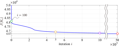
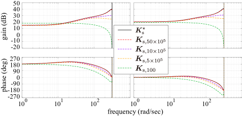
We first investigate the global convergence of the model-based PGM (16) with (26). We choose in (16). In Fig. 1, the blue solid line shows the variation of the cost in (11) for the iteration , while the black dotted line shows the optimal cost , where is given by (13). In addition, for each of the updated gains indicated by the colored circles in Fig. 1, we construct in (2) based on Lemma 2. Similarly, we construct from . Fig. 2 shows the variation of the Bode diagrams of those controllers. We can see from Figs. 1-2 that the PGM (16) with (26) successfully updates the dynamical controller so that its control performance is close to optimal. The resultant output feedback controller indicated by the red dotted line in Fig. 2 is
|
|
(54) |
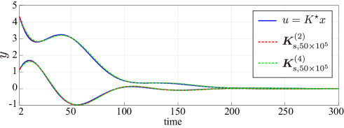
Let this controller be denoted as . In Fig. 3, the red dotted lines show the trajectory of in (1) when is actuated at , whereas the blue solid lines show the case when the state-feedback controller is actuated at , where is defined as in (12). Note that is generated by the aforementioned and the initial input . By comparing these lines, we can see that the learned output feedback dynamical controller exhibits optimal performance equivalent to that of the state-feedback controller.
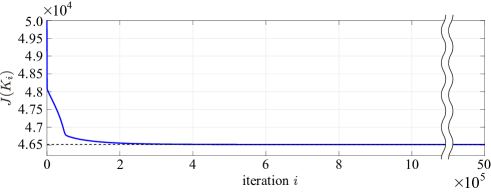
Moreover, the global convergence property of the PGM holds even if we choose to be unnecessarily large. Let and the other settings be the same as above. Fig. 4 shows the variation of in this case. Let the dynamical controller corresponding to the learned gain at be denoted as . In Fig. 3, the green dotted lines show the trajectory of when this controller is actuated at . We can see from Figs. 3-4 that the PGM with a different choice of can also find a global optimal solution.
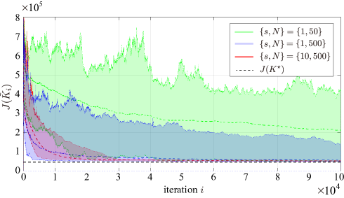
Next, we investigate the effectiveness of the multi-episodic PGM, i.e., Algorithm 1. Let , and . Suppose that we always execute Step 4). We consider three cases: , and execute the algorithm 50 times for each case. In Fig. 5, the green, blue, and red areas show the ranges covered by the 50 different variations of for each case, while the broken colored lines are the averages of the corresponding 50 variations. In addition, the broken black line shows the optimal cost. This figure implies that the larger or is, the smaller the difference in performance improvement per iteration. Further, we can see that the controller adaptation to an optimal controller is successful for any choices of and as iterations continue.
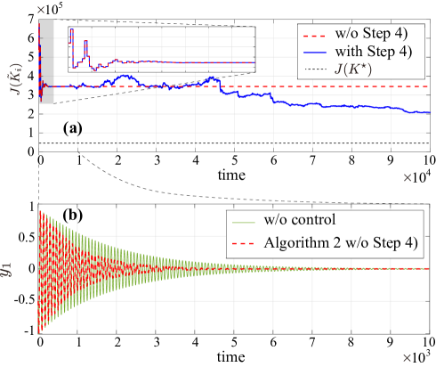
Finally, we investigate the effectiveness of the single-episodic PGM, i.e., Algorithm 2, where and . First, we suppose that Step 4) in the algorithm is skipped at every iteration. In Fig. 6(a), the red dotted line shows the variation of with respect to the time but not the iteration . We can see that the performance improves as increases. Furthermore, Fig. 6(b) shows how the transient response of is improved by the algorithm; the green solid line shows the case when no control is actuated, whereas the red dotted line shows the case corresponding to the red dotted line in Fig. 6(a). As demonstrated in this simulation, Algorithm 2 is not only a data-driven method for finding a better dynamical controller, but also an adaptive controller by itself to improve performance. However, the performance improvement stops for . This is because, in addition to the fact that (51) was not satisfied, the state almost converged, as described in Remark 6. To break away from there, we execute Step 4) in Algorithm 2 if for . Let the additive excitation signal follow with from to Also, to improve the convergence speed, we let . The variation of in this case is depicted by the blue solid lines in Fig. 6. We can see that the performance improvement successfully restarts and gradually becomes closer to a global optimum. These results imply the effectiveness of the proposed model-based/model-free PGMs.
VI Conclusion
In this paper, we have proposed model-based/model-free PGMs for designing dynamic output feedback controllers for discrete-time partially observable systems, using the newly introduced IOH dynamics and the corresponding reachability-based lossless projection. Unlike in SOF control [18, 19, 20, 12], the global linear convergence of the PGMs is guaranteed with a high probability (which becomes one for the model-based PGM) when design parameters are appropriately chosen. Future work includes establishing a computable criteria from data for parameter selection. Another task is to apply the proposed single-episodic PGM to more realistic systems, such as power systems.
-A Proof of Lemma 1
| (55) |
Hence, from a simple calculation, we have the output equation in (5). The dynamics of (5) follows from the definition of . This shows that and obey (5). From (52), any satisfies (53). From the reachability of , the subspace spanned by for any and input signals is . Note that this holds without depending on and . Hence,
| (56) |
which yields (7). Note that . Hence, . This completes the proof.
-B Proof of Lemma 2
We first show the equivalence of the two open-loop systems and for a common input . Let in (8) be denoted by , and the IOH generated by (8) be denoted by for . Hence, (8) is described as for , and is described as . We show for . From (2), we have
By substituting into this, we have . Hence, . Further, similarly to the proof of Lemma 1, it follows from (2) that for . Therefore, for , which shows the equivalence between and . Further, and are equivalent from Lemma 1. This completes the proof.
-C Proof of Proposition 1
We first show
| (57) |
From the proof of Lemma 1, holds for . Further, because due to , (57) holds. Based on this relation, we show the claim. To this end, we define the value function described as
|
|
(58) |
where obeys (5). Note from optimal control theory [24] that the minimizer in (58) is described as the linear controller , . Hence, , where is defined as (11). We will show that . From Lemma 1, without loss of generality, in (58) can be assumed to obey (1). Hence, from optimal control theory, the function has the form of while the minimizer in (58) is described as for , where is defined as (12). By combining this with (57), we have (13). Finally, we show that satisfies in Proposition 1. Note that holds when . By substituting into (58), the Bellman equation (58) is rewritten as
| (59) |
Here, from (10) and (18), there exists such that . From (19) and the relation , it follows that for . Since is reachable, must satisfy . Therefore, is invertible. Hence, (59) yields . This completes the proof.
-D Proof of Lemma 3
The existence of satisfying (18) follows from Lemma 1. Next, we show (19). Define such that is a unitary matrix. Define and . Then, the dynamics in (5) can be written as
| (60) |
It follows from (7) that . Hence, the dynamics in (19) follows. Finally, we have . This shows (19). From (19), we have . Hence, . The positive definiteness of immediately follows from (10). This completes the proof.
-E Proof of Lemma 5
We define
| (61) |
By pre- and post-multiplying and by (22), and by using the relation (24), we have
Note that holds for any because of (7) and (18). By substituting the above to (61), at can be written as
Similarly to Lemma 1 in [11], by differentiating at and taking the expectation of the derived equation, we obtain the claim.
-F Proof of Lemma 6
The sufficiency is obvious. We show the necessity. Note that
for where and is the Kronecker product. Hence, we have where ; is defined in (20). Further, using the notation
| (62) |
for given , the cost can be written as . Note that . Thus, yields , which shows the stability of . This completes the proof.
-G Proof of Lemma 7
The invertibility of follows from , where is defined in (20). Consider in (61), and in (25). Note that for . Define , , and for . It follows from the above that
Hence, we have
| (63) | |||
| (64) |
where appendix C.1 of [11] is used for deriving (63). Further, it follows from that is written as
| (65) |
Hence, in (26) can be written as
| (66) |
Further, it follows from the first equation that
| (67) |
Using (65)-(66), we can rewrite (64) as
| (68) | |||||
Finally, by substituting (67) into (68) and using , the claim follows.
-H Proof of Lemma 8
Similarly to Lemma 7.9 of [12], for any we have the operator norm of the Hessian as
| (69) |
where is defined in Lemma 7 and is defined in (24). Because (30) is equivalent to [25], it suffices to show that the RHS of (69) is bounded by . Note that from the first equation in (23) and (20). Hence, for any , it follows that
| (70) |
We next show an upper bound of . Given , consider in (62). Similarly to the proof of Lemma 6, we have . Hence, for any . Note here that . Hence, we have . Further, yields . Hence,
| (71) |
holds. By substituting (70)-(71) into (69), we have , which completes the proof.
-I Preliminary lemmas for sample complexity analysis
Lemma 10
Proof
The proof consists of the following two steps:
-
i)
First, assuming that satisfies both (73) and , we show that
(74) (75) (76) -
ii)
Second, we show that satisfying (73) yields by reductio ad absurdum.
First, we show (74). To this end, assume . Because , for any there exists
We denote the identity operator as . In addition, we define the operator norm of as . To simplify the notation, we define and . As shown in Lemma 18 of [11] and the proof of Lemma 20 in [11], it follows that and
| (77) |
Further, we have
| (78) |
In addition, . Therefore, in what follows, we will derive upper bounds of , , and to show (74). Now, we have
where is defined in (21) and . Since holds from (73), we have
Hence, it follows that
| (79) |
Also, from Lemma 17 of [11] and (71), we have
| (80) |
Using (79) and (80), it follows that
| (81) |
In addition, from (73), we have
| (82) |
By substituting this into (81), we have
| (83) |
Using (77) and (83), similarly to the proof of Lemma 20 in [11], we have
| (84) |
Therefore, by substituting this, (79), and (80) into the final equation in (78), we have
| (85) |
Taking in (85) and using (71), we have (74). Next, we show (75). Using (74), we have
By substituting (82) into the final inequality, we have (75). Next, we show (76). From Lemma 23 of [11], we have
Thus, it follows that
this yields (76).
Finally, we move to step ii), i.e., show by reductio ad absurdum. Assume that there exists such that satisfies (73). Since the spectral radius is a continuous function, there exists on the path between and such that holds. Moreover, because is on the path, satisfies (73) with the replacement of by . Hence, . On the other hand,
follows. This is a contradiction. Therefore, it follows that any satisfying (73) is a stabilizing controller, i.e., . This completes the proof.
Lemma 11
Proof
Note that satisfies (73). Hence, follows, where in (72). Because , for any , there exists
Similarly, exists. In addition, follows from (23). Thus, we have
| (87) |
Define . Then, it follows for that
| (88) |
In what follows, we show upper bounds of the four operator norms in the RHS of (88).
First, we show
| (89) |
Let the unit eigenvector corresponding to the largest eigenvalue of be denoted as . It follows that
which yields (89).
Second, we show
| (90) |
Similarly to (78), using the notations and , we have
| (91) |
Similarly, we have
| (92) |
Thus, using (89), we have
|
|
(93) |
Since follows (86), we have . Hence, we have . Substituting this, (89), and (93) into the RHS of (91), we have (90).
Third, we show
| (94) |
This relation follows from
and .
Fourth, we show
| (95) |
This follows from .
-J Proof of Lemma 9
Note that (86) holds by choosing and , where is defined as in (36) because is smaller than in (9). Hence, ; thus, is Schur.
For any , let denote the initial IOH of the -th episode. Let and denote uniform distributions over and , respectively. Define
| (99) | |||
| (100) | |||
| (101) |
where is defined in (38). It follows that
| (102) |
We derive upper bounds of the three terms in the RHS of (102) as follows.
First, we show that a bound of the second term is given as
| (103) |
To this end, let
|
, |
(104) |
and show that
| (105) |
holds for any , where . Let and . It holds that
Further, we have
Hence, follows. Thus, we have . By substituting the fact that and (71) into this relation, we have (105). Note that (95) holds. In addition, (105) follows because . Hence,
holds, where the relation given in (105) is used to derive the second final inequality. Thus, it follows that
| (106) |
This shows (103).
Second, we show
| (107) |
Note from Lemma 1 of [26] that
holds. Because , holds from Lemma 11. Hence, (30) holds for and , which is equivalent to . Thus, by using Jensen’s inequality, we have
| (108) |
which yields (107).
Third, we show
| (109) |
holds for any . To this end, we use the following Bernstein’s inequality:
Proposition 2 (Corollary 6.2.1 of [27])
Let satisfy and . Also, let be the -th random independent copy of and define . Then, for any , it follows that
| (110) |
where .
We utilize this proposition to show (109). More specifically, we define
Then, and in the proposition become and . From Lemma 11, (98) holds when and . Hence . Further, because holds from (9), we have . Hence, using the fact that if , we have
| (111) |
Thus, . Note that this inequality holds for any . Thus, we can choose as in Proposition 2. Also, we have
Hence, we can choose as in the proposition. Finally, note that holds if . Thus, by choosing as in the proposition, we have (109).
-K Proof of Theorem 2
First, we show Claim i). Note that for any and that is continuous around a positive neighborhood at . Hence, Claim i) follows.
Next, we show
|
|
(112) |
for any and such that . To this end, we show
| (113) |
where is defined in (72). From Theorem 1, we have with , which yields . Since for any , we have
with a probability of at least . By letting and in Lemma 10, the relation (73) holds because holds. Therefore, (113) holds. Now, we prove (112). Let . From the proof of Lemma 11 in [11], it follows
where is defined in Lemma 7, in (66), and . Note here that . Hence,
|
|
From the proof of Lemma 11 and the fact that , the relation (97) holds with a probability of at least when and . Hence, it follows that
| (114) |
with a probability of at least . On the other hand, it follows that
| (115) |
Note that if and . By adding (115) into (114), (112) holds for any . Finally, by letting be , we have (49). This completes the proof.
References
- [1] Z. S. Hou and Z. Wang, “From model-based control to data-driven control: Survey, classification and perspective,” Information Sciences, vol. 235, pp. 3–35, 2013.
- [2] M. C. Campi, A. Lecchini, and S. M. Savaresi, “Virtual reference feedback tuning: a direct method for the design of feedback controllers,” Automatica, vol. 38, no. 8, pp. 1337–1346, 2002.
- [3] F. L. Lewis and D. Liu, Reinforcement learning and approximate dynamic programming for feedback control. John Wiley & Sons, 2013.
- [4] C. D. Persis and P. Tesi, “Formulas for data-driven control: Stabilization, optimality, and robustness,” IEEE Transactions on Automatic Control, vol. 65, no. 3, pp. 909–924, 2019.
- [5] H. Hjalmarsson, M. Gevers, and F. De Bruyne, “For model-based control design, closed-loop identification gives better performance,” Automatica, vol. 32, no. 12, pp. 1659–1673, 1996.
- [6] M. Lorenzen, M. Cannon, and F. Allgöwer, “Robust MPC with recursive model update,” Automatica, vol. 103, pp. 461–471, 2019.
- [7] V. Krishnan and F. Pasqualetti, “On direct vs indirect data-driven predictive control,” in Proc. of Conference on Decision and Control, 2021, pp. 736–741.
- [8] H. J. Van Waarde, J. Eising, H. L. Trentelman, and M. K. Camlibel, “Data informativity: a new perspective on data-driven analysis and control,” IEEE Transactions on Automatic Control, vol. 65, no. 11, pp. 4753–4768, 2020.
- [9] S. Oymak and N. Ozay, “Non-asymptotic identification of LTI systems from a single trajectory,” in Proc. of American control conference, 2019, pp. 5655–5661.
- [10] R. S. Sutton and A. G. Barto, Reinforcement learning: An introduction (Second Edition). MIT press, 2018.
- [11] M. Fazel, R. Ge, S. Kakade, and M. Mesbahi, “Global convergence of policy gradient methods for the linear quadratic regulator,” in Proc. of International Conference on Machine Learning. PMLR, 2018, pp. 1467–1476.
- [12] J. Bu, A. Mesbahi, M. Fazel, and M. Mesbahi, “LQR through the lens of first order methods: Discrete-time case,” arXiv, 2019.
- [13] H. Mohammadi, A. Zare, M. Soltanolkotabi, and M. R. Jovanović, “Global exponential convergence of gradient methods over the nonconvex landscape of the linear quadratic regulator,” in Proc. of Conference on Decision and Control, 2019, pp. 7474–7479.
- [14] H. Mohammadi, M. Soltanolkotabi, and M. R. Jovanovic, “Random search for learning the linear quadratic regulator,” in Proc. of American Control Conference, 2020, pp. 4798–4803.
- [15] H. Mohammadi, A. Zare, M. Soltanolkotabi, and M. R. Jovanović, “Convergence and sample complexity of gradient methods for the model-free linear–quadratic regulator problem,” IEEE Transactions on Automatic Control, vol. 67, no. 5, pp. 2435–2450, 2021.
- [16] V. Gullapalli, “A stochastic reinforcement learning algorithm for learning real-valued functions,” Neural networks, vol. 3, no. 6, pp. 671–692, 1990.
- [17] S. K. Mishra and G. Giorgi, Invexity and optimization. Springer Science & Business Media, 2008.
- [18] I. Fatkhullin and B. Polyak, “Optimizing static linear feedback: Gradient method,” SIAM Journal on Control and Optimization, vol. 59, no. 5, pp. 3887–3911, 2021.
- [19] S. Takakura and K. Sato, “Structured output feedback control for linear quadratic regulator using policy gradient method,” arXiv, 2022.
- [20] J. Bu, A. Mesbahi, and M. Mesbahi, “On topological and metrical properties of stabilizing feedback gains: the MIMO case,” arXiv, 2019.
- [21] J. Duan, W. Cao, Y. Zheng, and L. Zhao, “On the optimization landscape of dynamical output feedback linear quadratic control,” arXiv, 2022.
- [22] T. Sadamoto and O. Kaneko, “Data-dependent analysis of model validation errors for linear system identification,” European Journal of Control, vol. 66, pp. 1–10, 2022.
- [23] B. Polyak, “Gradient methods for the minimisation of functionals,” Ussr Computational Mathematics and Mathematical Physics, vol. 3, pp. 864–878, Dec. 1963.
- [24] F. L. Lewis, D. Vrabie, and V. L. Syrmos, Optimal control. John Wiley & Sons, 2012.
- [25] S. Boyd and L. Vandenberghe, Convex optimization. Cambridge university press, 2004.
- [26] A. D. Flaxman, A. T. Kalai, and H. B. McMahan, “Online convex optimization in the bandit setting: gradient descent without a gradient,” arXiv preprint cs/0408007, 2004.
- [27] J. A. Tropp, An Introduction to Matrix Concentration Inequalities. Foundations and Trends in Machine Learning, 2015.