Resolving Fock states near the Kerr-free point of a superconducting resonator

Abstract

We have designed a tunable nonlinear resonator terminated by a SNAIL (Superconducting Nonlinear Asymmetric Inductive eLement). Such a device possesses a sweet spot in which the external magnetic flux allows to suppress the Kerr interaction. We have excited photons near this Kerr-free point and characterized the device using a transmon qubit. The excitation spectrum of the qubit allows to observe photon-number-dependent frequency shifts about nine times larger than the qubit linewidth. Our study demonstrates a compact integrated platform for continuous-variable quantum processing that combines large couplings, considerable relaxation times and excellent control over the photon mode structure in the microwave domain.

Encoding quantum information in the infinite Hilbert space of a harmonic oscillator is a promising avenue for quantum computing. Recently, significant progress has been made by using three-dimensional (3D) microwave cavities Ma et al. (2020); Hu et al. (2019); Reinhold et al. (2020); Grimm et al. (2020); Gertler et al. (2021); Gao et al. (2018). Thanks to the strong-dispersive coupling, quantum states such as cat states Vlastakis et al. (2013); Wang et al. (2016), GKP states Campagne-Ibarcq et al. (2020) and the cubic phase state Kudra et al. (2022) have been engineered. However, currently, the scalability and connectivity is difficult, limited by the size of the cavity. Another simpler method is to use coplanar microwave resonators where resonators and qubits can be fabricated together in a single chip Schuster et al. (2007); Wang et al. (2008); Hofheinz et al. (2008). The drawback is the shorter relaxation time of coplanar resonators compared to 3D cavities.

Both 2D and 3D microwave resonators as well as acoustic resonators Chu et al. (2018); Andersson et al. (2019) host linear modes. Therefore, an ancillary qubit is customarily used to introduce a nonlinearity for state preparation and operation. However, the limited coherence of the ancillary qubit and the imperfect operations on it will decrease the fidelity of the actual states Heeres et al. (2015, 2017); Kudra et al. (2022). To avoid operations on ancillary qubits, a Superconducting QUantum Interference Device (SQUID) can be used to terminate a coplanar resonator. This not only provides the tunability of the mode frequency by changing the external magnetic flux through the loop Wallquist et al. (2006); Mahashabde et al. (2020); Kennedy et al. (2019); Palacios-Laloy et al. (2008); Vissers et al. (2015); Sandberg et al. (2008), it also induces a sufficiently nonlinearity. Using this nonlinearity, experiments in waveguide quantum electrodynamics have demonstrated the generation of entangled microwave photons by the parametrical pumping of a symmetrical SQUID loop Schneider et al. (2020); Sandbo Chang et al. (2018). Non-Gaussian states, regarded as a resource for quantum computing, have also been realized Chang et al. (2020); Agustí et al. (2020); Wang et al. (2019). Therefore, state preparation and operations can be implemented in a nonlinear resonator, even without ancillary qubits. However, in those experiments, the generated states can not be stored for a long time since the resonators are directly coupled to the waveguides.

Theoretically, it has been shown that pulsed operations on a novel tunable nonlinear resonator can be used to achieve a universal gate set for continuous-variable (CV) quantum computation Hillmann et al. (2020). The proposed device is similar to a parametric amplifier where the Josephson junction or SQUID loop is replaced by an asymmetric Josephson device known as the SNAIL (Superconducting Nonlinear Asymmetric Inductive eLement) Frattini et al. (2018); Sivak et al. (2019), is applied. Using a SNAIL or an asymmetrically threaded SQUID loop Lescanne et al. (2020); Miano et al. (2022), it is possible to realize three-wave mixing free of residual Kerr interactions by biasing the element at a certain external magnetic flux. In this work, we refer to this flux sweet spot as the Kerr-free point.

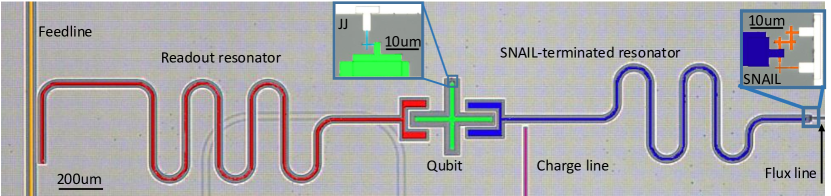
Figure 1: A scanning optical micrograph of the measured sample. A superconducting qubit with a cross-shaped island (green) and a single Josephson junction (JJ, light blue in the middle inset), capacitively coupled to both a coplanar read-out resonator (red) and the nonlinear resonator (blue). The nonlinear resonator is formed by a linear coplanar resonator terminated by a superconducting nonlinear asymmetric inductive element (SNAIL) that has three big Josephson junctions and one small junction (orange in right inset). The charge line (pink) is used to operate the qubit and drive the nonlinear resonator. The qubit state read-out is implemented through the transmission of the feedline. The on-chip flux line is not used in this work, instead, a superconducting coil on the top of the chip [not shown] is used to generate the external magnect flux $\Phi_{\rm{ext}}$ through the SNAIL. See more fabrication details and the measurement setup for this device in Supplementary.

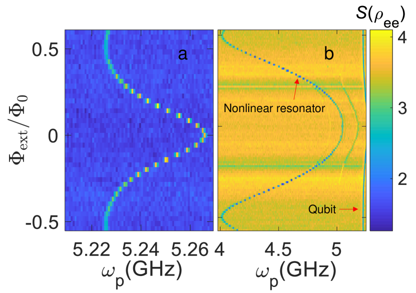
Figure 2: Spectroscopy for the qubit frequency and the SNAIL-terminated resonator frequency. a, The qubit frequency vs. the external magnetic flux through the SNAIL. b, The SNAIL-terminated resonator frequency vs. the external magnetic flux through the SNAIL. The nonlinear resonator is dispersively coupled to the qubit as shown in Fig. 1. $S(\rho_{\rm{ee}})\propto\rho_{\rm{ee}}$ is the measured signal from the read-out pulse of the qubit. $\omega_{\rm p}$ is the probe frequency.

Therefore, it is meaningful to investigate a SNAIL-terminated resonator in circuit quantum electrodynamics (cQED) where the nonlinear resonator, decoupled to the waveguide, can be used for state preparation and storage. Strong dispersive coupling between oscillators and qubits was achieved a decade ago for photons Schuster et al. (2007) and recently for phonons  Sletten et al. (2019); Arrangoiz-Arriola et al. (2019); von Lüpke et al. (2021), in linear resonators. Here, we observed the very well-resolved photon-number splitting up to the $9^{\rm{th}}$-photon Fock state in a SNAIL-terminated resonator coupled to a qubit. Our nonlinear resonator has a considerable relaxation time up to $T_{1}=20\,\rm\mu s$ under a few-photon drive, limited by (Two-Level Systems) TLSs. Our study opens the door to implement, operate and store quantum states on this scalable platform in the future. Moreover, compared to a linear resonator, our resonator has a non-negligible dephasing rate from its high sensivity to the magnetic flux noise due to the SNAIL loop.

Table 1: SNAIL-terminated resonator parameters at zero magnetic flux and near the Kerr-free point. The values are extracted from a transmission coefficient measurement on a SNAIL-terminated resonator coupled to a transmission line. We have $\gamma_{\rm{s}}=1/T_{\rm{s}}=\omega_{\rm s}/Q_{\rm{s}}$ where $\gamma_{\rm{s}}$, $T_{\rm{s}}$, $\omega_{\rm s}$ and $Q_{\rm{s}}$ are the resonator intrinsic decoherence rate, coherence time, frequency and the internal Q value, respectively. The intrinsic decoherence rate is given by $\gamma_{\rm{s}}=\frac{\Gamma_{1}}{2}+\Gamma_{\phi}$ where the intrinsic relaxation rate $\Gamma_{1}=\frac{1}{T_{1}}$ with the lifetime $T_{1}$ and the pure dephasing rate $\Gamma_{\phi}=\frac{1}{T_{\phi}}$ with the pure dephasing time $T_{\phi}$.

$\Phi_{\rm{ext}}/\Phi_{0}$	$\omega_{\rm s}/2\pi$	$Q_{\rm{s}}$	$\gamma_{\rm{s}}/2\pi$	$T_{\rm{s}}$
	$\rm{GHz}$		$\rm{kHz}$	$\mu$s
0	5.14	$2.23\times 10^{5}$	23	6.92
0.386	4.31	$3.86\times 10^{4}$	112	1.42

Characterization of the SNAIL-terminated resonator. In order to characterize the parameters for the SNAIL-terminated resonator directly, we first fabricated a SNAIL-terminated $\lambda/2$ resonator capacitively coupled to a coplanar transmission line [not shown], which is the same as the nonlinear resonator in Fig. 1. By measuring the transmission coefficient through a vector network analyzer similar to measuring conventional resonators Verjauw et al. (2021); Calusine et al. (2018); Kowsari et al. (2021); Probst et al. (2015), at the 10 mK stage of a dilution refrigerator, we can extract the nonlinear resonator frequency at different external magnetic fluxes [see Supplementary]. For our SNAIL-terminated resonator, the inductive energy can be written as Hillmann et al. (2020); Frattini et al. (2018); Sivak et al. (2019)

$$U_{\rm{SNAIL}}(\phi)=-\beta E_{\rm{J}}\cos(\phi)-3E_{\rm{J}}\cos\big{(}\frac{\phi_{\rm{ext}}-\phi}{3}\big{)},$$ (1)

where $\beta$ is the ratio of the Josephson energies of the small and the big junctions of the SNAIL, $\phi$ is the superconducting phase across the small junction, $\phi_{\rm{ext}}=2\pi\Phi_{\rm{ext}}/\Phi_{0}$ is the reduced external magnetic flux, and $E_{\rm{J}}$, related to the Josephson inductance $L_{\rm{J}}$, is the Josephson energy of the big junctions in the SNAIL. Upon quantization, the Hamiltonian for the SNAIL-terminated resonator becomes

$$H_{\rm{s}}=\hbar\omega_{\rm{s}}+g_{3}(a+a^{\dagger})^{3}+g_{4}(a+a^{\dagger})^{4},$$ (2)

where $g_{3}$ ($g_{4}$) is the couplings for the three (four)-wave mixing coupling strength, and $\omega_{s}$ is the resonator frequency which follows the relation Hillmann et al. (2020)

$$\omega_{\rm{s}}\tan{\big{(}\frac{\pi}{2}\frac{\omega_{\rm{s}}}{\omega_{\rm{r}0}}\big{)}}=\frac{Z_{c}c_{2}}{3L_{J}},$$ (3)

where $\omega_{\rm{r}0}$ describes the bare resonance frequency of the resonator without the SNAIL, $Z_{c}=58.7\,\Omega$ for the characteristic impedance of the resonator, and $c_{2}$ is a numerically determinable coefficient for the linear coupling whose specific value depends on $\beta$ and $\phi_{\rm{ext}}$ in our case.

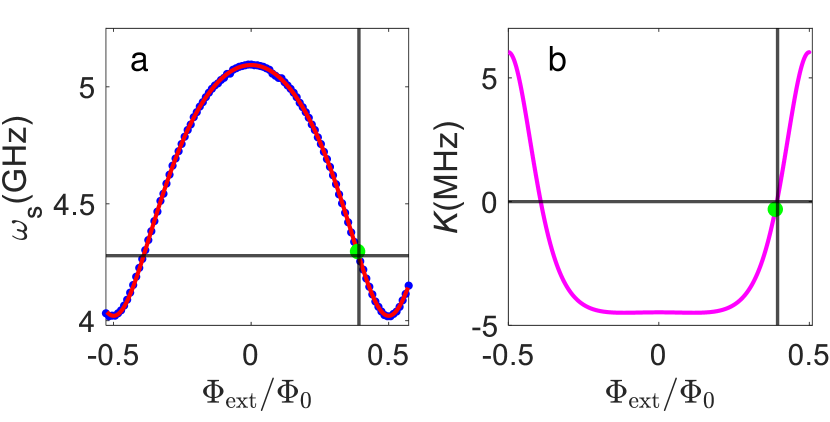
Figure 3: Frequency and Kerr strength for SNAIL-terminated resonator coupled to a qubit. a, The frequency of the nonlinear resonator vs. the external magnetic flux through the SNAIL. Blue dots (red curve) are (is) the experimental (fitting) data. By fitting the data to Eq. 3 [red curve], we obtain $\beta=0.9993\pm 0.0005$, well matched with the resistance ratio of the big junction over the small junction 0.104, measured at room temperature, $L_{\rm{J}}=629\pm 8\,\rm pH$ and $\omega_{\rm{s}}=8.87\pm 0.07\,\rm GHz$. The crossed point from two blacklines indicate the corresponding resonator frequency at the Kerr-free point. b, The Kerr-frequency shift per photon, $\it{K}$, vs. the external magnetic flux through the SNAIL calculated from the parameters in a. The crossed point from two black lines indicates that the Kerr coefficient is zero at $\Phi_{\rm{ext}}=0.392~{}\Phi_{0}$. The green dot at $\Phi_{\rm{ext}}=0.386~{}\Phi_{0}$ is the operating flux point in our work.

By sending a very weak probe with the average photon number in the resonator from the probe much less than one, we measure the corresponding transmission coefficient to extract the internal $Q_{\rm{s}}$ values at $\Phi_{\rm{ext}}=0$ and $\Phi_{\rm{ext}}=0.386~{}\Phi_{0}$ close to the Kerr-free point, where the magnetic flux is calibrated using the flux period $\Phi_{\rm{0}}$ of the SNAIL-terminated resonator frequency. As shown in Table. 1, we find that the coherence time in both cases is above one microsecond, especially, $T_{\rm{s}}\approx 7\mu s$ at $\Phi_{\rm{ext}}=0$. When we tune the resonator to $\Phi_{\rm{ext}}=0.386~{}\Phi_{0}$t, the coherence time is reduced by a factor of five due to the pure dephasing from the magnetic flux noise through the SNAIL.

A SNAIL-terminated resonator coupled to a qubit. In order to verify the nonlinear resonator performance in cQED in Fig. 1, the nonlinear resonator is dispersively coupled to a fixed frequency superconducting qubit with the bare qubit frequency $\frac{\omega_{\rm{q0}}}{2\pi}\approx 5.222\,\rm GHz$. The effective Hamiltonian that contains the leading order corrections to the rotating wave approximation for describing the coupled SNAIL-terminated resonator and qubit in the dispersive regime ($g_{0}\ll\Delta_{0}$) Noguchi et al. (2020) is

$$\frac{H_{\rm{eff}}}{\hbar}\approx\omega_{\rm{c}}a^{\dagger}a+K{a^{{\dagger}2}}a^{2}+\frac{\omega_{\rm{q}}}{2}b^{\dagger}b-\frac{\chi_{0}}{2}a^{\dagger}ab^{\dagger}-\frac{\alpha_{q}}{2}b^{\dagger 2}b^{2},$$

(4)

where the bare SNAIL-terminated resonator is dispersively shifted to be $\omega_{\rm c}=\omega_{\rm{s}}-\frac{g_{0}^{2}}{\Delta_{0}}$, and the qubit frequency for the qubit mode $b$ is $\omega_{\rm q}=\omega_{\rm q0}+\frac{g_{0}^{2}}{\Delta_{0}}$ with the bare qubit frequency $\omega_{\rm q0}$ and the Stark shift $\frac{g_{0}^{2}}{\Delta_{0}}$. $g_{0}$ is the coupling strength between the nonlinear resonator and the qubit, and $\Delta_{0}=\omega_{\rm q0}-\omega_{\rm s}$ is the detuning between the resonator and the bare qubit frequencies. The dispersive shift is $\chi_{0}=\frac{g_{0}^{2}\alpha_{\rm{q}}}{\Delta_{0}(\Delta_{0}-\alpha_{\rm{q}})}$ with the qubit anharmonicity $\alpha_{\rm{q}}\approx 450\,\rm MHz$. Furthermore, near the Kerr-free point where the Kerr nonlinearity (strength $K$) is cancelled in the leading order, the residual Kerr nonlinearity is due to the interplay of four- and three-wave mixing processes Hillmann et al. (2020) as well as the qubit induced nonlinearity.

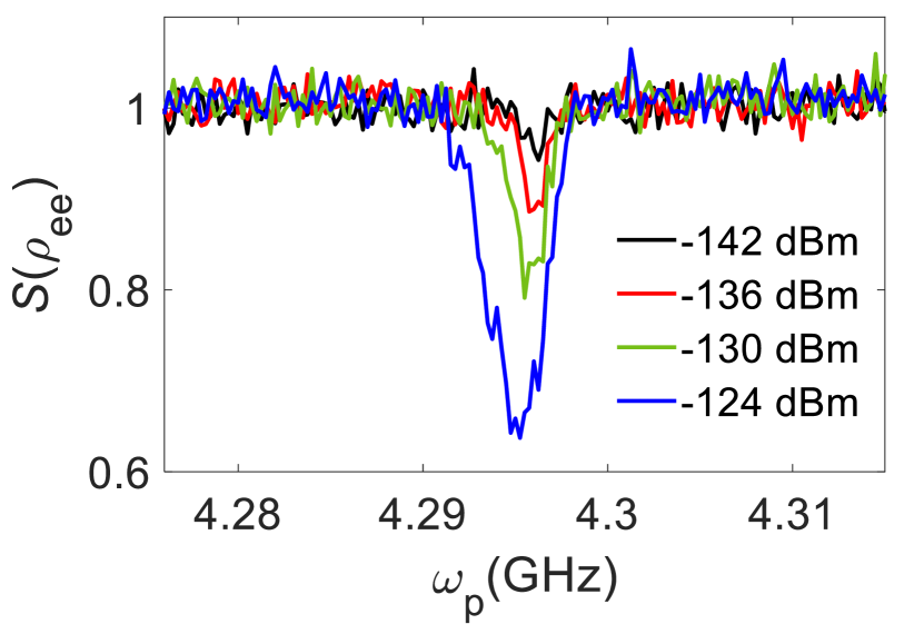
Figure 4: The spectroscopy of the nonlinear resonator near the Kerr-free point with different input powers. The signal $S(\rho_{\rm{ee}})$ is from the readout pulse, depending on the qubit population $\rho_{\rm{ee}}$ where $\rho_{\rm{ee}}$ is determined by the nonlinear resonator photon population. $\omega_{\rm{p}}$ is the frequency of the continuous probe where we vary the probe power to the sample from $-142\,\rm dBm$ to $-124\,\rm dBm$. The dip indicates the resonator frequency. The full linewidth of the dip is also reduced from about 10 MHz to 3 MHz. Note that the dip linewidth is almost three orders of magnitude larger than the resonator linewidth. At the lowest pump power, we find the qubit-dressed resonator frequency is $\omega_{\rm c}/2\pi\approx 4.296\,\rm GHz$.

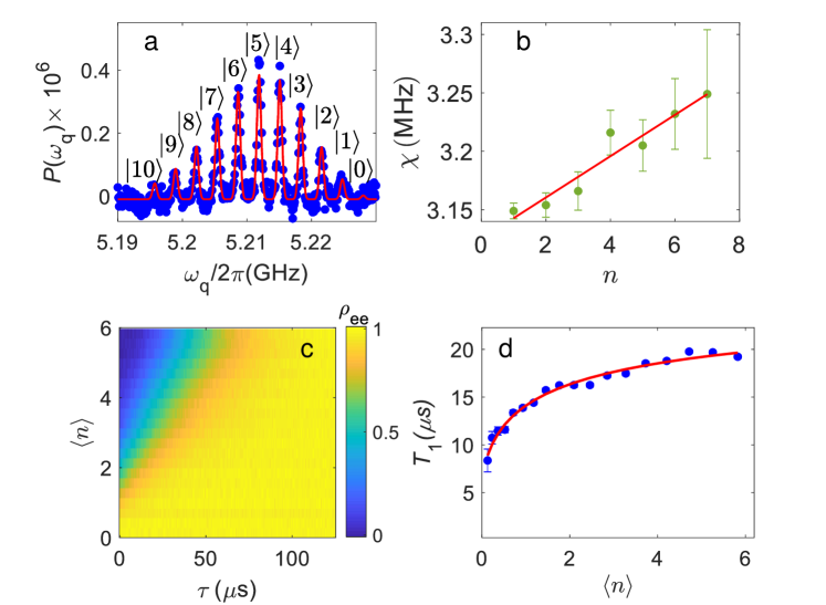
Figure 5: Photon-number splitting and lifetime of the SNAIL-terminated resonator near the Kerr-free point. a, the qubit-frequency distribution $P(\omega_{\rm{q}})=P(\omega_{\rm{q}})\times 10^{6}$ with the average photon number $|\alpha|^{2}\approx 6$, of the coherent displacement in the nonlinear resonator. The envelope of the distribution matches well with a Poisson distribution with the corresponding coherent-state amplitude $|\alpha|\approx 2.4$ [red solid line]. b, Dispersive shift $\chi$ over different photon numbers $n$ inside the nonlinear resonator. The data is fitted to the equation $\chi=\chi_{0}+\chi^{\prime}(n-1)/2$ with $\chi_{0}/2\pi=3.143\pm 0.021\,\rm MHz$ and the higher order correction $\chi^{\prime}/2\pi=35\pm 11\,\rm kHz$. c, the qubit population $\rho_{\rm{ee}}$ depending on the photon number $\langle n\rangle=|\alpha|^{2}$ in the nonlinear resonator. $\tau$ is the waiting time after the short displacement before the qubit read-out. d, The relaxation time $T_{1}$ of the nonlinear resonator vs. different photon number $\langle n\rangle$ inside the resonator. The error bars are for the standard deviation.

To experimentally find the qubit frequency, we sweep the frequency of a qubit-excitation pulse with the pulse length $\tau_{\rm{p}}=1\,\rm\mu s$ (spectroscopy pulse, see pulse generation in Supplementary). When the nonlinear resonator frequency is changed by the external flux $\Phi_{\rm{ext}}$, the values of $\Delta_{0}$ and the qubit frequency are also changed. In Fig. 2a, at a fixed $\Phi_{\rm{ext}}$, we sweep the pulse frequency, and when the pulse is on resonance with the qubit, the qubit is excited. Then, we measure the qubit state by sending a readout pulse to obtain $S(\rho_{\rm{ee}})\propto\rho_{\rm{ee}}$, which is manifested as bright dots in Fig. 2a. After finding the qubit frequency and calibrating the corresponding $\pi$-pulses at different values of $\Phi_{\rm{ext}}$, we send a continuous coherent drive to the nonlinear resonator meanwhile driving the qubit on resonance. However, when the drive is on resonance with the nonlinear resonator, the resonator is populated, leading to a change of the qubit frequency due to the dispersive interaction. Thus, the $\pi$-pulse will not excite the qubit anymore, resulting in a smaller signal $S(\rho_{\rm{ee}})$ [Fig. 2b].

With the values of $\omega_{\rm q0}$ and the dressed-qubit frequencies [Fig. 2a], we can obtain the values of the Stark shift at different external magnetic fluxes. Therefore, we can compensate the Stark shift from the qubit onto the SNAIL-terminated resonator to obtain the bare resonator frequency $\omega_{\rm s}$ [blue dots in Fig. 3a from Fig. 2b]. With the parameters extracted from Fig. 3a, we can calculate the Kerr coefficient as a function of external magnetic flux [pink curve in Fig. 3b, see Supplementary]. At the device operation point $\Phi_{\rm{ext}}=0.386\,\rm\Phi_{0}$ [green dot in Fig. 3b], close to the Kerr-free point $\Phi_{\rm{ext}}=0.386~{}\Phi_{0}$, we deduce a residual Kerr at the operation point of $K=-0.31\pm 0.04\,\rm MHz$ with $g_{3}/2\pi=-11.6\pm 0.4\,\rm MHz$, and $g_{4}/2\pi=-0.128\pm 0.004\,\rm MHz$.

Due to the dispersive coupling to the qubit, the qubit can be used as a very efficient probe to determine the frequency of the SNAIL-terminated resonator. In our case, the linewidth of the nonlinear resonator is only a few kHz. Thus, it will be extremely difficult to find the resonator frequency based on the reflection coefficient measurement Lu et al. (2021a, b, b, 2022); Lin et al. (2020) through the charge line. However, since our qubit is coupled to the resonator with a dispersive shift up to a few MHz as shown in Fig. 5c, a few photons inside the resonator will shift the qubit frequency significantly. Consequently, even though the frequency detuning between the pump frequency and the resonator frequency is much larger than the linewidth of the resonator, as soon as the intensity of the pump is strong enough to inject a few photons inside the resonator, we can perform qubit spectroscopy to roughly find the resonator frequency. Afterwards, we can find the resonator frequency more accurately by decreasing the pump intensity [Fig. 4].

Photon-number splitting near the Kerr-free point. Once we have determined the nonlinear resonator frequency, we perform a pump-probe measurement consisting of a short pulse (50 ns) to excite the resonator followed by a long qubit excitation pulse with $\tau_{\rm{p}}=2\,\rm\mu s$ and frequency $\omega_{\rm q}$, along with a read-out pulse at the end to infer the qubit excited-state population. Due to the weak hybridization between the qubit and the nonlinear resonator near the Kerr-free point, the short coherent pulse drives the resonator into an approximately coherent state with amplitude $|\alpha|$. We observed the qubit frequency splitting with the Fock states up to 9 photons where each peak has a Gaussian shape due to the quantum fluctuation of the photon number inside the resonator Gambetta et al. (2006) [Fig. 5a]. The separation of each peak is about 3 MHz, ten times larger than the qubit linewidth $\frac{\gamma_{\rm{q}}}{2\pi}\approx 280\,\rm kHz$, leading to well-resolved peaks. The pulse length satisfies $\tau_{\rm{p}}\gg 1/\gamma$, resulting in a good frequency resolution.

From the peak difference of the qubit spectroscopy [see Supplementary], we can extract the dispersive shift which increases with the photon number [Fig. 5b]. According to the dispersive shift $\chi_{0}$ and the qubit anharmonicity $\alpha_{\rm{q}}$, we can obtain the coupling strength $g_{0}/2\pi\approx 53\,\rm MHz$. Moreover, near the Kerr-free point, the self-Kerr $K_{\rm{sq}}$ of the SNAIL-resonator induced by the qubit-resonator coupling Hillmann and Quijandría (2022); Noguchi et al. (2020) is $K_{\rm{sq}}=-24g_{4}g_{0}^{2}/\Delta_{0}^{2}\approx-2\pi\times 9\,\rm kHz$, which is more than three hundred times smaller than the dispersive shift and more than 10 times smaller than $\gamma_{\rm{s}}$. Thus, the residual Kerr coefficient from the qubit has a small influence on the states stored in our device, which can be also completely suppressed by slightly shifting the external flux $\Phi_{\rm{ext}}$.

Lifetime of a single photon in the nonlinear resonator near the Kerr-free point. Even though a statistic study can be done by measuring multiple resonators coupled to waveguides to infer the average lifetime, it is still important to study the relaxation time directly on a specific device in cQED since in reality the device performance varies over different devices due to the imperfect fabrication process.

Here, for the device shown in Fig. 1, utilizing the dispersive coupling to the qubit, we can determine the energy lifetime of the nonlinear resonator $T_{1}$ at the single-photon level. Again, we send a 50 ns pulse to displace the resonator with the initial amplitude $|\alpha(\tau=0)|$, and after a time delay $\tau$, we apply a conditional $\pi$-pulse where the pulse is on resonance with the qubit frequency when the resonator is empty. Therefore, the qubit-excitation population depends on the photon number $\langle n\rangle$. In Fig. 5c at $\tau\sim 0$, when $\langle n\rangle<1$, the qubit frequency is still mainly centered at $\omega_{\rm q}/2\pi=5.228\,\rm GHz$, leading to the qubit population $\rho_{\rm{ee}}\approx 1$. However when $\langle n\rangle>1$, the qubit frequency starts to split, leading to a decreased $\rho_{\rm{ee}}$ where the population goes to zero smoothly and reaches $\rho_{\rm{ee}}\approx 0$ with $\langle n\rangle=5.8$. However, with increasing $\tau$, the coherent field in the resonator decreases as $\alpha(\tau)=\alpha(0){\rm{exp}}(-\tau/(2T_{1}))$ and the qubit frequency moves back. Thus, the conditional pulse can excite the qubit again.

Two-level systems (TLSs) are investigated extensively using conventional coplanar resonators Woods et al. (2019); Calusine et al. (2018); Wenner et al. (2011); Burnett et al. (2014); de Graaf et al. (2020); Brehm et al. (2017); McRae et al. (2020) along waveguides, where the photon number inside the resonator can be only roughly estimated according to the attenuation of the setup, and there is no TLS study in cavity quantum electrodynamics. Here, thanks to the accurate calibration of the photon number inside the nonlinear resonator, it is possible to directly study the TLS effect on our nonlinear resonator. The value of $T_{1}$ in Fig. 5d, extracted from the data in Fig. 5c [see Supplementary], increases from $8\,\rm\mu s$ to $20\,\rm\mu s$, which can be explained by saturation of two-level systems (TLS). According to the TLS model McRae et al. (2020); Burnett et al. (2014); Gao (2008), the resonator internal $Q_{1}$ is given by

$$\frac{1}{Q_{1}}=\frac{1}{\omega_{\rm c}T_{1}}=F\delta_{\rm{TLS}}\frac{\tanh{\big{(}\frac{\hbar\omega_{\rm c}}{2k_{\rm{B}}T_{\rm{res}}}\big{)}}}{\sqrt{1+\frac{\langle n\rangle}{n_{\rm{c}}}}}+\delta_{\rm{other}},$$ (5)

where $F$ is the filling factor describing the ratio of electrical field in the TLS host volume to the total volume. $\delta_{\rm{TLS}}$ is the TLS loss tangent of the dielectric hosting the TLSs, $n_{\rm{c}}$ is the critical photon number within the resonator to saturate one TLS. $\delta_{\rm{other}}$ is the contribution from non-TLS loss mechanisms. A fit to Eq. (5) gives $F\delta_{\rm{TLS}}\approx 4.5\times 10^{-6}$, $\delta_{\rm{other}}\approx 1.3\times 10^{-6}$ and $n_{\rm{c}}\approx 0.1$ photons [red solid curve in Fig. 5d], which is several orders of magnitude smaller than for normal linear resonators Burnett et al. (2018, 2014); Brehm et al. (2017); McRae et al. (2020); Kowsari et al. (2021); Verjauw et al. (2021); Calusine et al. (2018). This can be explained by long-lived TLSs due to $n_{\rm{c}}\propto\sqrt{T_{1,\rm{TLS}}T_{2,\rm{TLS}}}$ Gao (2008). Additionally, we also analyse the non-TLS loss where the loss could be possibly from both the chip design and chip modes [See supplementary].

Compared to the coherence time of the SNAIL-terminated resonator coupled to a waveguide near the Kerr-free point, the relaxation time here is significantly larger, indicating that the coherence time is limited by the pure dephasing. Assuming that the resonator coupled to the waveguide has the same internal relaxation time as the nonlinear resonator coupled to a qubit, according to $1/T_{\rm{s}}=1/(2T_{1})+1/T_{\phi}$ with $T_{1}\approx 8~{}\mu s$ at $\langle n\rangle\approx 0$ from Fig. 5d, we can infer the pure dephasing time $T_{\phi}\approx 12\,\rm\mu s$ and $2\,\rm\mu s$ at $\Phi_{\rm{ext}}=0$ and $\Phi_{\rm{ext}}=0.386~{}\Phi_{0}$, respectively. Especially, at $\Phi_{\rm{ext}}=0.386~{}\Phi_{0}$, the resonator becomes much more sensitive to the magnetic flux noise, leading to a shorter coherence time which could be increased by reducing the SNAIL parameter $\beta$ or adding more magnetic shielding to suppress the magnetic-flux noise or decrease the loop size.

In this study, we developed an efficient method to characterize a SNAIL-terminated nonlinear resonator and observed well-resolved photon-number splitting up to nine photons, where the relaxation time can be up to $20\,\rm\mu s$. The parameters of our device are suitable for implementing universal gate sets for quantum computing Hillmann et al. (2020). Compared to linear modes coupled to qubits, in our case, the Kerr effect from the ancilla qubit can be suppressed, leading to a better storage of bosonic modes where the Kerr coefficient makes the quantum state collapse Kirchmair et al. (2013). Moreover, by taking the advantages of the nonlinearity of our resonator, we could also generate and store entangled photon modes and non-Gaussian states Chang et al. (2020); Agustí et al. (2020). The dispersive coupling between the qubit and the resonator could also enable us to make quantum state tomography very efficient. Finally, compared to 3D cavities, our chip-scale structure is more compact for integration and scalability required by the large-scale CV quantum processing in the future.

Supplementary

Experimental setup. The complete experimental setup is shown in Fig. 6. The sample, as shown in Fig.1 in the main text, is wire-bonded in a nonmagnetic oxygen-free cooper sample box, mounted to the 10 mK stage of a dilution refrigerator, and shielded by a $\mu$-metal can which is used for suppressing the static and fluctuating magnetic field. The signal to the qubit and the SNAIL-terminated resonator, with heavily attenuation, is combined to the charge line on the sample. A pulse is sent to the feedline on the sample to read out the state of the qubit with amplification using a traveling-wave parametric amplifier (TWPA) at the 10 mK stage, a high electron mobility transistor (HEMT) amplifier at 3 K and a room-temperature amplifier.

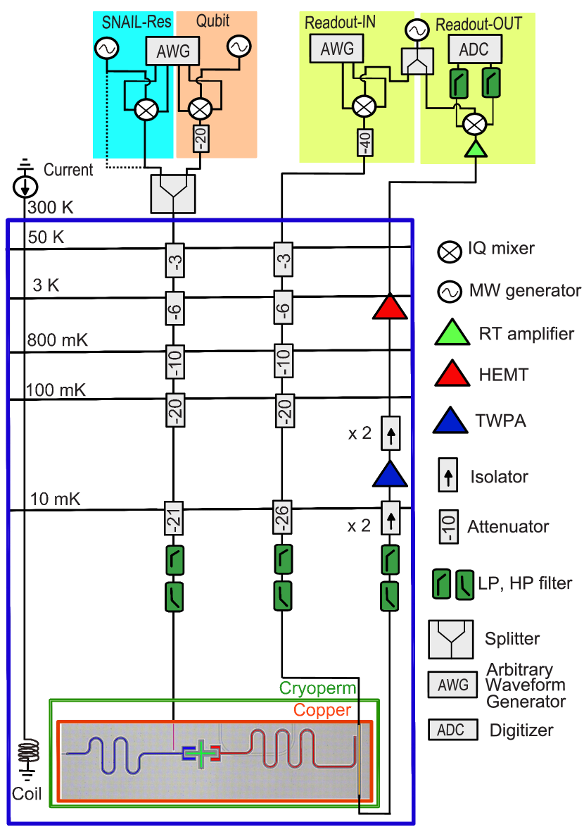
Figure 6: Experimental setup. Complete wiring diagram and room temperature setup for the nonlinear resonator coupled to a qubit. The qubit operation and the pulsed displacement are made by analog upconversion of the pulsed generated by an AWG (blue and orange). The dashed line in the blue box means that sometimes the microwave generator is connected to the combiner to pump the resonator continuously. The qubit readout (yellow) is controlled by the up- and down- conversion of a pulse generated by an AWG, and then digitized by an analog to digital converter (ADC).

Sample Fabrication. We first clean a high-resistance ($10\,\rm k\Omega$) 2-inch silicon wafer by hydrofluoric acid with $2\%$ concentration. Then, we evaporate aluminum on top of the silicon substrate, followed by direct laser writing, and etching using wet chemistry to obtain all the sample details except the Josephson junction. The Josephson junctions for the qubit and the SNAIL are defined in a bi-layer resist stack using electron-beam lithography. Later, we deposit aluminum again by using a two-angle evaporation technique. In order to ensure a superconducting contact between the junctions and the rest of circuit, an argon ion mill is used to remove native aluminium oxide before the junction aluminium deposition. Finally, the wafer is diced into individual chips and cleaned properly using both wet and dry chemistry.

Device parameters for the SNAIL-terminated resonator coupled to the waveguide. By sending a microwave probe to the SNAIL-terminated resonator coupled to the waveguide [the device for Table I in the main text], we measure the transmission coefficient of a SNAIL-terminated resonator to obtain the bare resonator frequency [blue stars in Fig. 7(a)]. Then, we get $\beta=0.095$ and $E_{\rm{J}}/(2\pi\hbar)=\frac{\hbar}{4e^{2}L_{\rm{J}}}\approx 830\,\rm GHz$ with the Josephson inductance $L_{\rm{J}}=600\,\rm pH$ by fitting the data to Eq.(3) in the main text [solid curve]. In Fig. 7(b), based on the values of $E_{\rm{J}}$ and $\beta$, we numerically calculate the Kerr coefficient $K$ due to the four-wave mixing coupling, which $K$ can be suppressed to zero at the flux point $\Phi_{\rm{ext}}/\Phi_{0}=0.39$.

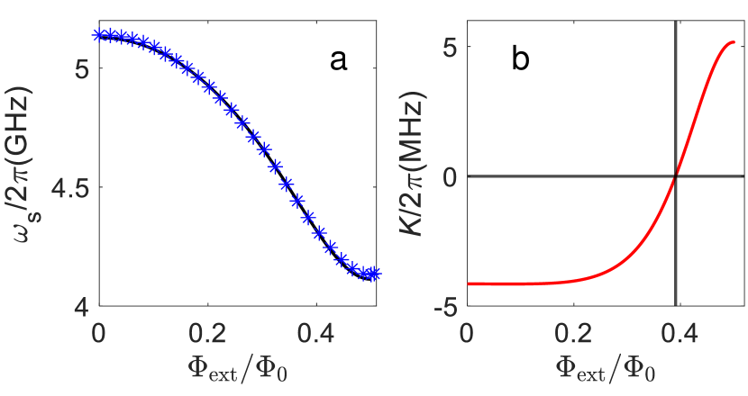
Figure 7: Frequency and Kerr strength for a SNAIL-terminated resonator coupled to a waveguide. a, The frequency of the nonlinear resonator vs. the external magnetic flux through the SNAIL. Stars are the experimental data determined from the transmission coefficient of the vector analyzer network. The solid blue curve is calculated numerically. b, The Kerr-frequency shift per photon, $\sf{K}$, vs. the external magnetic flux through the SNAIL. The Kerr-free point occurs at $\Phi_{\rm{ext}}=0.39~{}\Phi_{0}$.

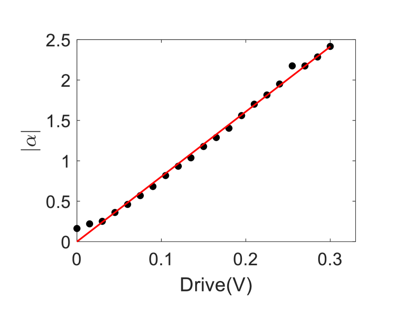
Figure 8: Pulse amplitude calibration. Calibration of the coherent displacement $\alpha$ with the voltage output $A$, of the arbitrary-wavefunction generator at the room-temperature.

Pulse generation and calibration. The microwave control for the qubit and the nonlinear resonator is achieved by up-converting the inphase (I) and the quadrature (Q) components of a low frequency pulse generated by four AWG channels (two each for the qubit and the resonator). The qubit read-out pulse is up-converted to the sample and then down-converted after the amplification with the same local oscillator (yellow area). The pump pulse for the displacement is generated by an IQ mixer with an input pulse from an Arbitrary Waveform Generator (AWG) with amplitude. In Fig. 8, we vary the amplitude of the pump pulse by changing the voltage amplitude $A$, and then obtain the corresponding displacement in the resonator according to the photon-number splitting as described in the main text. The data (black dots) is fitted to the equation $|\alpha|=kA$ with $k\approx 8$. This measurement is useful to calibrate the pump pulse with different amplitudes. We also notice that the residual thermal population with $A=0$ is $|\alpha|=0.16$ ($\langle n\rangle=|\alpha|^{2}\approx 0.03$ photons). The thermal and Poisson distributions are almost the same when the thermal photon number is small. In this case, we only take into account the single photon $P_{1}$ and the vacuum $P_{0}$ populations.Thus, we can calculate the corresponding thermal temperature as $T_{\rm{res}}=\hbar\omega_{\rm c}/\big{[}k_{\rm{B}}\ln{\big{(}1+\frac{1}{\langle n\rangle}}\big{)}\big{]}\approx 58\,\rm mK$. Kerr coefficient calculation. According the extracted parameters $\beta$ and $L_{\rm{J}}$ from Fig. 3a in the main text, we can calculate the coefficients $g_{3}$ and $g_{4}$ for the three-wave mixing and four-wave mixing terms, respectively [Fig. 9]. Then, we can infer the coupling strength for the Kerr coefficient $K$ according to $K=12(g_{4}-5g_{3}^{2}/\omega_{\rm s})$ [Fig.3b in the main text]. Qubit spectroscopy. In order to increase the signal-to-noise ratio, here, we average the qubit spectroscopy with different driven voltages [Fig. 10a] to obtain Fig. 10b. Afterwards, each peak corresponding to a photon number is fitted to a Gaussian function to extract the dispersive shift as shown in Fig.5b in the main text.

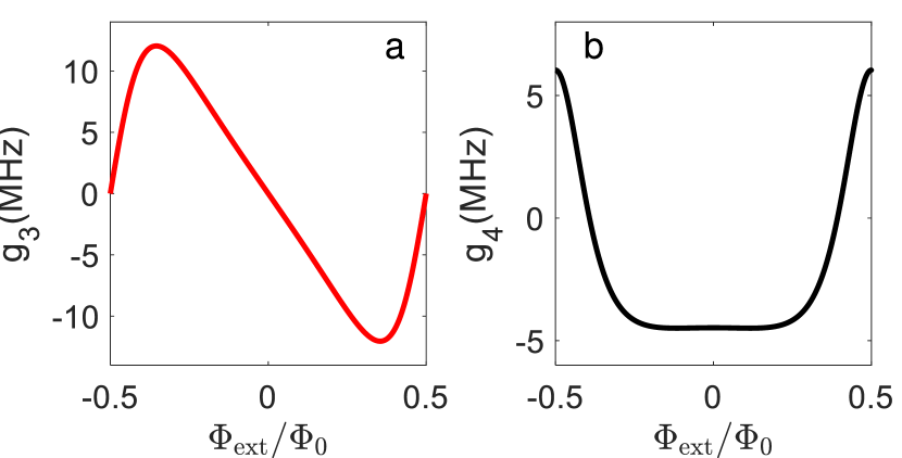
Figure 9: $g_{3}$ and $g_{4}$ numerical values for the SNAIL-terminated resonator coupled to a qubit. The numerical values of $g_{3}$ and $g_{4}$ for the SNAIL-terminated resonator coupled to a qubit.

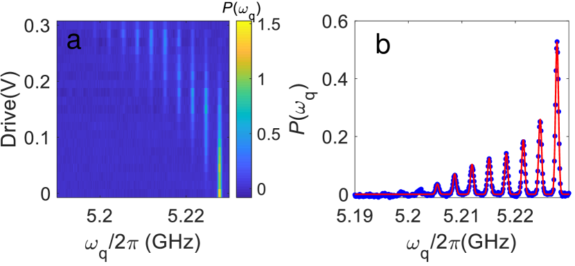
Figure 10: Qubit spectroscopy under different drive voltages. a, The qubit-frequency distribution $P(\omega_{\rm{q}})=P(\omega_{\rm{q}})\times 10^{6}$ Vs. different drive voltages. b, The averaged qubit-frequency distribution.

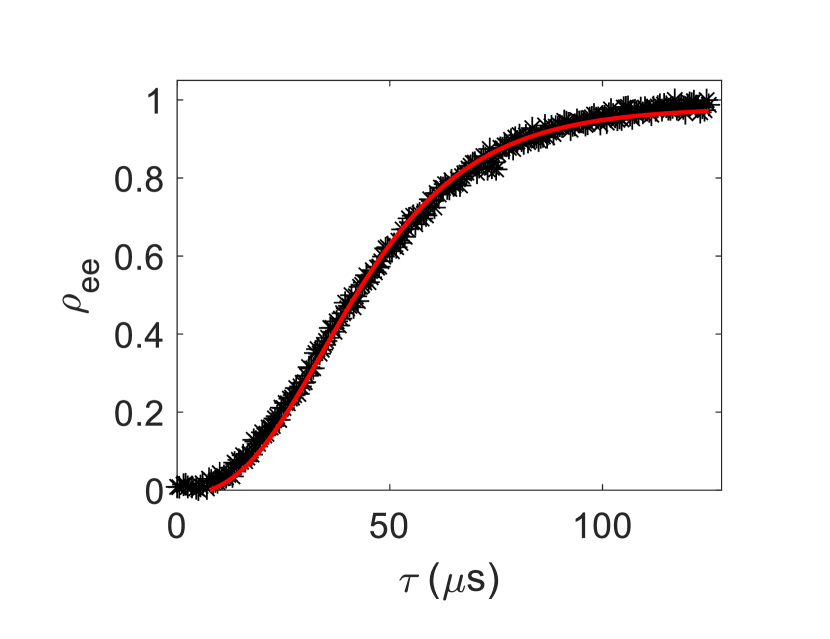
Figure 11: Extract the value of $T_{1}$ from the qubit population. The qubit population $\rho_{\rm{ee}}$ vs. the waiting time $\tau$ with $\langle n\rangle=5.8$.

The lifetime $T_{1}$ of the resonator. In Fig. 11, The data trace [black stars] is from the top trace in Fig.5c in the main text with the average photon number $\langle n\rangle=5.8$. Here, we show an example to obtain the value of $T_{1}$ from Fig.5c in the main text. The qubit excitation probability is $\rho_{\rm{ee}}=1-\rm{exp}[-|\alpha(0)|^{2}{\rm{exp}(-\tau/T_{1})}]$. By fitting the rising curve [Fig. 11] with the calibrated $|\alpha(0)|=\sqrt{5.8}$ $(\langle n\rangle=5.8)$ , we extract $T_{1}=19.2\pm 0.2\,\rm\mu s$, corresponding to a quality factor of $Q_{1}=\omega_{\rm c}T_{1}\approx 5.18\times 10^{5}$ which is close to the $Q_{1}$ value for a coplanar linear resonator in the few-photon limit Kowsari et al. (2021); Burnett et al. (2018). In order to improve $T_{1}$ further in the future, we also analyse the non-TLS loss. The non-TLS loss limits the lifetime to be $T_{\rm{other}}=1/(\delta_{\rm{other}}\omega_{\rm c})\approx 28\,\rm\mu s$ comparable to our qubit lifetime $T_{1,\rm{q}}\approx 20\,\rm\mu s$. In our sample, the nonlinear resonator couples to the qubit, charge line and a flux line where they contribute to the non-TLS loss as $\gamma_{\rm{q}}/2\pi=(g_{0}/\Delta_{0})^{2}\frac{1}{T_{1,\rm{q}}}\approx 170\,\rm Hz$, $\gamma_{\rm{c}}/2\pi\approx 2.07\,\rm kHz$ and $\gamma_{\rm{f}}/2\pi\approx 477\,\rm Hz$, respectively (the values of $\gamma_{\rm{c}}$ and $\gamma_{\rm{f}}$ are from the simulation). In total, the loss from the chip design is $\gamma_{\rm{total}}=\gamma_{\rm{q}}+\gamma_{\rm{c}}+\gamma_{\rm{f}}\approx 2\pi\times 2.717\,\rm kHz$ corresponding to $T_{\rm{total}}=1/\gamma_{\rm{total}}\approx 59{\,\rm\mu s}\approx 2T_{\rm{other}}$´, meaning that other unknown losses such as the chip modes are similiar to the loss from the chip design.

AUTHOR CONTRIBUTIONS

Y.L. planned the project. Y.L. performed the measurements with help from M.K. and J.Y.Y. Y.L. designed and fabricated the sample. T.H. and F.Q. helped to make the numerical calculation. Y.L. wrote the manuscript with input from all the authors. Y.L. analyzed the data. P.D. supervised this project.

COMPETING INTERESTS

The authors declare no competing interests.

REFEREENCES

References

- Ma et al. (2020) Yuwei Ma, Yuan Xu, Xianghao Mu, Weizhou Cai, Ling Hu, Weiting Wang, Xiaoxuan Pan, Haiyan Wang, YP Song, C-L Zou, and L.Sun, “Error-transparent operations on a logical qubit protected by quantum error correction,” Nature Physics 16, 827 (2020).
- Hu et al. (2019) Ling Hu, Yuwei Ma, Weizhou Cai, Xianghao Mu, Yuan Xu, Weiting Wang, Yukai Wu, Haiyan Wang, YP Song, C-L Zou, et al., “Quantum error correction and universal gate set operation on a binomial bosonic logical qubit,” Nature Physics 15, 503–508 (2019).
- Reinhold et al. (2020) Philip Reinhold, Serge Rosenblum, Wen-Long Ma, Luigi Frunzio, Liang Jiang, and Robert J Schoelkopf, “Error-corrected gates on an encoded qubit,” Nature Physics 16, 822 (2020).
- Grimm et al. (2020) Alexander Grimm, Nicholas E Frattini, Shruti Puri, Shantanu O Mundhada, Steven Touzard, Mazyar Mirrahimi, Steven M Girvin, Shyam Shankar, and Michel H Devoret, “Stabilization and operation of a kerr-cat qubit,” Nature 584, 205 (2020).
- Gertler et al. (2021) Jeffrey M Gertler, Brian Baker, Juliang Li, Shruti Shirol, Jens Koch, and Chen Wang, “Protecting a bosonic qubit with autonomous quantum error correction,” Nature 590, 243 (2021).
- Gao et al. (2018) Yvonne Y Gao, Brian J Lester, Yaxing Zhang, Chen Wang, Serge Rosenblum, Luigi Frunzio, Liang Jiang, SM Girvin, and Robert J Schoelkopf, “Programmable interference between two microwave quantum memories,” Physical Review X 8, 021073 (2018).
- Vlastakis et al. (2013) Brian Vlastakis, Gerhard Kirchmair, Zaki Leghtas, Simon E Nigg, Luigi Frunzio, Steven M Girvin, Mazyar Mirrahimi, Michel H Devoret, and Robert J Schoelkopf, “Deterministically encoding quantum information using 100-photon schrödinger cat states,” Science 342, 607 (2013).
- Wang et al. (2016) Chen Wang, Yvonne Y Gao, Philip Reinhold, Reinier W Heeres, Nissim Ofek, Kevin Chou, Christopher Axline, Matthew Reagor, Jacob Blumoff, KM Sliwa, et al., “A schrödinger cat living in two boxes,” Science 352, 1087 (2016).
- Campagne-Ibarcq et al. (2020) Philippe Campagne-Ibarcq, Alec Eickbusch, Steven Touzard, Evan Zalys-Geller, Nicholas E Frattini, Volodymyr V Sivak, Philip Reinhold, Shruti Puri, Shyam Shankar, Robert J Schoelkopf, et al., “Quantum error correction of a qubit encoded in grid states of an oscillator,” Nature 584, 368 (2020).
- Kudra et al. (2022) Marina Kudra, Mikael Kervinen, Ingrid Strandberg, Shahnawaz Ahmed, Marco Scigliuzzo, Amr Osman, Daniel Pérez Lozano, Mats O. Tholén, Riccardo Borgani, David B. Haviland, Giulia Ferrini, Jonas Bylander, Anton Frisk Kockum, Fernando Quijandría, Per Delsing, and Simone Gasparinetti, “Robust preparation of wigner-negative states with optimized snap-displacement sequences,” PRX Quantum 3, 030301 (2022).
- Schuster et al. (2007) DI Schuster, Andrew Addison Houck, JA Schreier, A Wallraff, JM Gambetta, A Blais, L Frunzio, J Majer, B Johnson, MH Devoret, et al., “Resolving photon number states in a superconducting circuit,” Nature 445, 515 (2007).
- Wang et al. (2008) H. Wang, M. Hofheinz, M. Ansmann, R. C. Bialczak, E. Lucero, M. Neeley, A. D. O’Connell, D. Sank, J. Wenner, A. N. Cleland, and John M. Martinis, “Measurement of the decay of fock states in a superconducting quantum circuit,” Phys. Rev. Lett. 101, 240401 (2008).
- Hofheinz et al. (2008) Max Hofheinz, EM Weig, M Ansmann, Radoslaw C Bialczak, Erik Lucero, M Neeley, AD O?connell, H Wang, John M Martinis, and AN Cleland, “Generation of fock states in a superconducting quantum circuit,” Nature 454, 310 (2008).
- Chu et al. (2018) Yiwen Chu, Prashanta Kharel, Taekwan Yoon, Luigi Frunzio, Peter T Rakich, and Robert J Schoelkopf, “Creation and control of multi-phonon fock states in a bulk acoustic-wave resonator,” Nature 563, 666 (2018).
- Andersson et al. (2019) Gustav Andersson, Baladitya Suri, Lingzhen Guo, Thomas Aref, and Per Delsing, “Non-exponential decay of a giant artificial atom,” Nature Physics 15, 1123 (2019).
- Heeres et al. (2015) Reinier W. Heeres, Brian Vlastakis, Eric Holland, Stefan Krastanov, Victor V. Albert, Luigi Frunzio, Liang Jiang, and Robert J. Schoelkopf, “Cavity state manipulation using photon-number selective phase gates,” Phys. Rev. Lett. 115, 137002 (2015).
- Heeres et al. (2017) Reinier W Heeres, Philip Reinhold, Nissim Ofek, Luigi Frunzio, Liang Jiang, Michel H Devoret, and Robert J Schoelkopf, “Implementing a universal gate set on a logical qubit encoded in an oscillator,” Nat. Commun. 8, 1 (2017).
- Wallquist et al. (2006) Margareta Wallquist, VS Shumeiko, and Göran Wendin, “Selective coupling of superconducting charge qubits mediated by a tunable stripline cavity,” Phys, Rev. B 74, 224506 (2006).
- Mahashabde et al. (2020) Sumedh Mahashabde, Ernst Otto, Domenico Montemurro, Sebastian de Graaf, Sergey Kubatkin, and Andrey Danilov, “Fast tunable high--factor superconducting microwave resonators,” Phys. Rev. Applied 14, 044040 (2020).
- Kennedy et al. (2019) O.W. Kennedy, J. Burnett, J.C. Fenton, N.G.N. Constantino, P.A. Warburton, J.J.L. Morton, and E. Dupont-Ferrier, “Tunable superconducting resonator based on a constriction nano-squid fabricated with a focused ion beam,” Phys. Rev. Applied 11, 014006 (2019).
- Palacios-Laloy et al. (2008) Agustín Palacios-Laloy, Francois Nguyen, Francois Mallet, Patrice Bertet, Denis Vion, and Daniel Esteve, “Tunable resonators for quantum circuits,” Journal of Low Temperature Physics 151, 1034 (2008).
- Vissers et al. (2015) Michael R Vissers, Johannes Hubmayr, Martin Sandberg, Saptarshi Chaudhuri, Clint Bockstiegel, and Jiansong Gao, “Frequency-tunable superconducting resonators via nonlinear kinetic inductance,” Appl. Phys. Lett. 107, 062601 (2015).
- Sandberg et al. (2008) Martin Sandberg, CM Wilson, Fredrik Persson, Thilo Bauch, Göran Johansson, Vitaly Shumeiko, Tim Duty, and Per Delsing, “Tuning the field in a microwave resonator faster than the photon lifetime,” Appl. Phys. Lett. 92, 203501 (2008).
- Schneider et al. (2020) B. H. Schneider, A. Bengtsson, I. M. Svensson, T. Aref, G. Johansson, Jonas Bylander, and P. Delsing, “Observation of broadband entanglement in microwave radiation from a single time-varying boundary condition,” Phys. Rev. Lett. 124, 140503 (2020).
- Sandbo Chang et al. (2018) C. W. Sandbo Chang, M. Simoen, José Aumentado, Carlos Sabín, P. Forn-Díaz, A. M. Vadiraj, Fernando Quijandría, G. Johansson, I. Fuentes, and C. M. Wilson, “Generating multimode entangled microwaves with a superconducting parametric cavity,” Phys. Rev. Applied 10, 044019 (2018).
- Chang et al. (2020) C. W. Sandbo Chang, Carlos Sabín, P. Forn-Díaz, Fernando Quijandría, A. M. Vadiraj, I. Nsanzineza, G. Johansson, and C. M. Wilson, “Observation of three-photon spontaneous parametric down-conversion in a superconducting parametric cavity,” Phys. Rev. X 10, 011011 (2020).
- Agustí et al. (2020) A. Agustí, C. W. Sandbo Chang, F. Quijandría, G. Johansson, C. M. Wilson, and C. Sabín, “Tripartite genuine non-gaussian entanglement in three-mode spontaneous parametric down-conversion,” Phys. Rev. Lett. 125, 020502 (2020).
- Wang et al. (2019) Zhaoyou Wang, Marek Pechal, E. Alex Wollack, Patricio Arrangoiz-Arriola, Maodong Gao, Nathan R. Lee, and Amir H. Safavi-Naeini, “Quantum dynamics of a few-photon parametric oscillator,” Phys. Rev. X 9, 021049 (2019).
- Hillmann et al. (2020) Timo Hillmann, Fernando Quijandría, Göran Johansson, Alessandro Ferraro, Simone Gasparinetti, and Giulia Ferrini, “Universal gate set for continuous-variable quantum computation with microwave circuits,” Phys. Rev. Lett. 125, 160501 (2020).
- Frattini et al. (2018) N. E. Frattini, V. V. Sivak, A. Lingenfelter, S. Shankar, and M. H. Devoret, “Optimizing the nonlinearity and dissipation of a snail parametric amplifier for dynamic range,” Phys. Rev. Applied 10, 054020 (2018).
- Sivak et al. (2019) V.V. Sivak, N.E. Frattini, V.R. Joshi, A. Lingenfelter, S. Shankar, and M.H. Devoret, “Kerr-free three-wave mixing in superconducting quantum circuits,” Phys. Rev. Applied 11, 054060 (2019).
- Lescanne et al. (2020) Raphaël Lescanne, Marius Villiers, Théau Peronnin, Alain Sarlette, Matthieu Delbecq, Benjamin Huard, Takis Kontos, Mazyar Mirrahimi, and Zaki Leghtas, “Exponential suppression of bit-flips in a qubit encoded in an oscillator,” Nature Physics 16, 509 (2020).
- Miano et al. (2022) A Miano, G Liu, VV Sivak, NE Frattini, VR Joshi, W Dai, L Frunzio, and MH Devoret, “Frequency-tunable kerr-free three-wave mixing with a gradiometric snail,” Applied Physics Letters 120, 184002 (2022).
- Sletten et al. (2019) L. R. Sletten, B. A. Moores, J. J. Viennot, and K. W. Lehnert, “Resolving phonon fock states in a multimode cavity with a double-slit qubit,” Phys. Rev. X 9, 021056 (2019).
- Arrangoiz-Arriola et al. (2019) Patricio Arrangoiz-Arriola, E Alex Wollack, Zhaoyou Wang, Marek Pechal, Wentao Jiang, Timothy P McKenna, Jeremy D Witmer, Raphaël Van Laer, and Amir H Safavi-Naeini, “Resolving the energy levels of a nanomechanical oscillator,” Nature 571, 537 (2019).
- von Lüpke et al. (2021) Uwe von Lüpke, Yu Yang, Marius Bild, Laurent Michaud, Matteo Fadel, and Yiwen Chu, “Parity measurement in the strong dispersive regime of circuit quantum acoustodynamics,” arXiv:2110.00263 (2021).
- Verjauw et al. (2021) J. Verjauw, A. Potočnik, M. Mongillo, R. Acharya, F. Mohiyaddin, G. Simion, A. Pacco, Ts. Ivanov, D. Wan, A. Vanleenhove, L. Souriau, J. Jussot, A. Thiam, J. Swerts, X. Piao, S. Couet, M. Heyns, B. Govoreanu, and I. Radu, “Investigation of microwave loss induced by oxide regrowth in high-q niobium resonators,” Phys. Rev. Applied 16, 014018 (2021).
- Calusine et al. (2018) Greg Calusine, Alexander Melville, Wayne Woods, Rabindra Das, Corey Stull, Vlad Bolkhovsky, Danielle Braje, David Hover, David K Kim, Xhovalin Miloshi, et al., “Analysis and mitigation of interface losses in trenched superconducting coplanar waveguide resonators,” Appl. Phys. Lett. 112, 062601 (2018).
- Kowsari et al. (2021) D Kowsari, K Zheng, JT Monroe, NJ Thobaben, X Du, PM Harrington, EA Henriksen, DS Wisbey, and KW Murch, “Fabrication and surface treatment of electron-beam evaporated niobium for low-loss coplanar waveguide resonators,” Appl. Phys. Lett. 119, 132601 (2021).
- Probst et al. (2015) Sebastian Probst, FB Song, Pavel A Bushev, Alexey V Ustinov, and Martin Weides, “Efficient and robust analysis of complex scattering data under noise in microwave resonators,” Rev. Sci. Instrum. 86, 024706 (2015).
- Noguchi et al. (2020) Atsushi Noguchi, Alto Osada, Shumpei Masuda, Shingo Kono, Kentaro Heya, Samuel Piotr Wolski, Hiroki Takahashi, Takanori Sugiyama, Dany Lachance-Quirion, and Yasunobu Nakamura, “Fast parametric two-qubit gates with suppressed residual interaction using the second-order nonlinearity of a cubic transmon,” Phys. Rev. A 102, 062408 (2020).
- Lu et al. (2021a) Yong Lu, Ingrid Strandberg, Fernando Quijandría, Göran Johansson, Simone Gasparinetti, and Per Delsing, “Propagating wigner-negative states generated from the steady-state emission of a superconducting qubit,” Phys. Rev. Lett. 126, 253602 (2021a).
- Lu et al. (2021b) Yong Lu, Andreas Bengtsson, Jonathan J Burnett, Emely Wiegand, Baladitya Suri, Philip Krantz, Anita Fadavi Roudsari, Anton Frisk Kockum, Simone Gasparinetti, Göran Johansson, et al., “Characterizing decoherence rates of a superconducting qubit by direct microwave scattering,” Npj Quantum Inf. 7, 35 (2021b).
- Lu et al. (2022) Yong Lu, Neill Lambert, Anton Frisk Kockum, Ken Funo, Andreas Bengtsson, Simone Gasparinetti, Franco Nori, and Per Delsing, “Steady-state heat transport and work with a single artificial atom coupled to a waveguide: Emission without external driving,” PRX Quantum 3, 020305 (2022).
- Lin et al. (2020) W-J Lin, Y Lu, PY Wen, Y-T Cheng, C-P Lee, K-T Lin, K-H Chiang, MC Hsieh, JC Chen, C-S Chuu, et al., “Deterministic loading and phase shaping of microwaves onto a single artificial atom,” https://arxiv.org/abs/2012.15084 (2020).
- Gambetta et al. (2006) Jay Gambetta, Alexandre Blais, D. I. Schuster, A. Wallraff, L. Frunzio, J. Majer, M. H. Devoret, S. M. Girvin, and R. J. Schoelkopf, “Qubit-photon interactions in a cavity: Measurement-induced dephasing and number splitting,” Phys. Rev. A 74, 042318 (2006).
- Hillmann and Quijandría (2022) Timo Hillmann and Fernando Quijandría, “Designing kerr interactions for quantum information processing via counterrotating terms of asymmetric josephson-junction loops,” Phys. Rev. Applied 17, 064018 (2022).
- Woods et al. (2019) W. Woods, G. Calusine, A. Melville, A. Sevi, E. Golden, D.K. Kim, D. Rosenberg, J.L. Yoder, and W.D. Oliver, “Determining interface dielectric losses in superconducting coplanar-waveguide resonators,” Phys. Rev. Applied 12, 014012 (2019).
- Wenner et al. (2011) James Wenner, R Barends, RC Bialczak, Yu Chen, J Kelly, Erik Lucero, Matteo Mariantoni, A Megrant, PJJ O?Malley, D Sank, et al., “Surface loss simulations of superconducting coplanar waveguide resonators,” Appl. Phys. Lett. 99, 113513 (2011).
- Burnett et al. (2014) Jonathan Burnett, Lara Faoro, I Wisby, VL Gurtovoi, AV Chernykh, GM Mikhailov, VA Tulin, R Shaikhaidarov, V Antonov, PJ Meeson, et al., “Evidence for interacting two-level systems from the 1/f noise of a superconducting resonator,” Nat. Commun. 5, 4119 (2014).
- de Graaf et al. (2020) SE de Graaf, L Faoro, LB Ioffe, S Mahashabde, JJ Burnett, T Lindström, SE Kubatkin, AV Danilov, and A Ya Tzalenchuk, “Two-level systems in superconducting quantum devices due to trapped quasiparticles,” Sci. Adv. 6, eabc5055 (2020).
- Brehm et al. (2017) Jan David Brehm, Alexander Bilmes, Georg Weiss, Alexey V Ustinov, and Jürgen Lisenfeld, “Transmission-line resonators for the study of individual two-level tunneling systems,” Appl. Phys. Lett. 111, 112601 (2017).
- McRae et al. (2020) Corey Rae Harrington McRae, Haozhi Wang, Jiansong Gao, Michael R Vissers, Teresa Brecht, Andrew Dunsworth, David P Pappas, and Josh Mutus, “Materials loss measurements using superconducting microwave resonators,” Rev. Sci. Instrum. 91, 091101 (2020).
- Gao (2008) Jiansong Gao, The physics of superconducting microwave resonators (PhD thesis, California Institute of Technology, 2008).
- Burnett et al. (2018) Jonathan Burnett, Andreas Bengtsson, David Niepce, and Jonas Bylander, “Noise and loss of superconducting aluminium resonators at single photon energies,” in J. Phys.: Conf. Ser., Vol. 969 (2018) p. 012131.
- Kirchmair et al. (2013) Gerhard Kirchmair, Brian Vlastakis, Zaki Leghtas, Simon E Nigg, Hanhee Paik, Eran Ginossar, Mazyar Mirrahimi, Luigi Frunzio, Steven M Girvin, and Robert J Schoelkopf, “Observation of quantum state collapse and revival due to the single-photon kerr effect,” Nature 495, 205 (2013).