Consistent Multiclass Algorithms for
Complex Metrics and Constraints

Abstract

We present consistent algorithms for multiclass learning with complex performance metrics and constraints, where the objective and constraints are defined by arbitrary functions of the confusion matrix. This setting includes many common performance metrics such as the multiclass G-mean and micro $F_{1}$-measure, and constraints such as those on the classifier’s precision and recall and more recent measures of fairness discrepancy. We give a general framework for designing consistent algorithms for such complex design goals by viewing the learning problem as an optimization problem over the set of feasible confusion matrices. We provide multiple instantiations of our framework under different assumptions on the performance metrics and constraints, and in each case show rates of convergence to the optimal (feasible) classifier (and thus asymptotic consistency). Experiments on a variety of multiclass classification tasks and fairness constrained problems show that our algorithms compare favorably to the state-of-the-art baselines.

Keywords: Multiclass, non-decomposable metrics, constraints, fairness, Frank-Wolfe, ellipsoid

1 Introduction

In many real-world machine learning tasks, the performance metric used to evaluate the performance of a classifier takes a complex form, and is not simply the expectation or sum of a loss on individual examples. Indeed, this is the case with the G-mean, H-mean and Q-mean performance metric used in class imbalance settings (Lawrence et al., 1998; Sun et al., 2006; Kennedy et al., 2009; Wang and Yao, 2012; Kim et al., 2013), the micro and macro $F_{1}$-measure used in information retrieval (IR) applications (Lewis, 1991), the worst-case error used in robust classification tasks (Vincent, 1994; Chen et al., 2017), and many others. Unlike linear performance metrics, which are simply linear functions (defined by a loss matrix) of the confusion matrix of a classifier, these complex performance metrics are defined by general functions of the confusion matrix. In this paper, we seek to design consistent learning algorithms for such complex performance metrics, i.e. algorithms that converge in the limit of infinite data to the optimal classifier for the metrics.

More generally, it is common for a classifier to be evaluated on more than one performance metric, and in such cases, a desirable goal could be to optimize the classifier’s performance on one metric while constraining the others to be within an acceptable range. These constrained classification problems commonly arise in fairness applications, where one may constrain a classifier to have equitable performance across multiple subgroups (Hardt et al., 2016; Zafar et al., 2017a), as well as, in many practical tasks where one wishes to constrain a classifier’s precision, coverage, or churn (Eban et al., 2017; Goh et al., 2016; Cotter et al., 2019b). Such metrics and constraints can be expressed as general functions of the confusion matrix, and are categorised as complex owing to their non-decomposable structure. Standard algorithmic learning frameworks are not readily designed to handle such complexity in the objectives and constraints. Doing so requires rethinking the underlying optimization schemes, as well as conducting bespoke analysis to establish algorithmic and statistical soundness. Practical applications and the lack of general approaches to solve such problems, motivate us to address the following question:

How can we design consistent algorithms for a general learning problem where the objective and (optionally) constraints are defined by general functions of the confusion matrix?

While there has been much interest in designing consistent algorithms for various types of supervised learning problems, most of this work has focused on linear performance metrics. This includes work on the binary or multiclass 0-1 loss (Bartlett et al., 2006; Zhang, 2004a, b; Lee et al., 2004; Tewari and Bartlett, 2007), losses for specific problems such as multilabel classification (Gao and Zhou, 2011), ranking (Duchi et al., 2010; Ravikumar et al., 2011; Calauzènes et al., 2012; Yang and Koyejo, 2020), and classification with abstention (Yuan and Wegkamp, 2010; Ramaswamy et al., 2018; Finocchiaro et al., 2020), and some work on general multiclass loss matrices (Steinwart, 2007; Ramaswamy and Agarwal, 2012; Pires et al., 2013; Ramaswamy et al., 2013; Nowak-Vila et al., 2020). The design of consistent algorithms for constrained classification problems has also received much attention recently, particularly in the context of fairness (Agarwal et al., 2018; Kearns et al., 2018; Donini et al., 2018), with the focus largely being on linear metrics and constraints.

There has also been much interest in designing algorithms for more complex performance metrics. One of the seminal approaches in this area is the $\text{SVM}^{\text{perf~{}}}$algorithm (Joachims, 2005), which was developed primarily for the binary setting. Other examples include convex relaxation based approaches that seek to improve upon the performance of this method (Kar et al., 2014, 2016; Narasimhan et al., 2019), as well as, algorithms for the binary $F_{1}$-measure and its multiclass and multilabel variants (Dembczynski et al., 2011, 2013; Natarajan et al., 2016; Zhang et al., 2020). Parallelly, there has been increasing interest in designing consistent algorithms for complex performance metrics. Most of these methods are focused on the binary case (Menon et al., 2013; Koyejo et al., 2014; Narasimhan et al., 2014; Dembczyński et al., 2017), and typically require tuning a single threshold or cost parameter to optimize the metric at hand. However, this simple approach of performing a one-dimensional parameter search does not extend easily to general $n$-class problems, where one may need to search over as many as $n^{2}$ parameters, requiring time exponential in $n^{2}$.

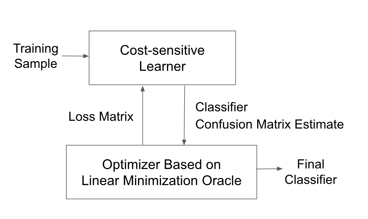
Figure 1: Simplified overview of the proposed framework.

In this paper, we develop a general framework for designing statistically consistent and computationally efficient algorithms for complex multiclass performance metrics and constraints. Our key idea is to pose the learning problem as an optimization problem over the set of feasible and achievable confusion matrices, and to solve this optimization problem using an optimization method that needs access to only a linear minimization routine (see Figure 1 for a simplified overview of the approach). Each of these linear minimization steps can be formulated as a cost-sensitive learning task, a classical problem for which numerous off-the-shelf solvers are available.

We provide instantiations of our framework under different assumptions on the performance metrics and constraints, and in each case establish rates of convergence to the optimal (feasible) classifier. Our algorithms can be used to learn plug-in type classifiers that post-shift a pre-trained class probability model, and are shown to be effective in optimizing for the given metric and constraints on a variety of application tasks.

1.1 Further Related Work

The literature on complex performance metrics and constrained learning can be broadly divided into two categories: algorithms that use surrogate relaxations (Joachims, 2005; Kar et al., 2014; Narasimhan et al., 2015a; Kar et al., 2016; Sanyal et al., 2018; Narasimhan et al., 2019), and algorithms that use a plug-in classifier (Ye et al., 2012; Menon et al., 2013; Koyejo et al., 2014; Narasimhan et al., 2014; Parambath et al., 2014; Dembczyński et al., 2017; Yang et al., 2020). The former methods are sometimes dubbed as in-training approaches, while the latter methods are referred to as post-hoc approaches.

A prominent example in the first category is the $\text{SVM}^{\text{perf~{}}}$ method of Joachims (2005), which employs a structural SVM formulation to construct convex surrogates for complex binary evaluation metrics. This approach does not however extend to multiclass problems as it uses a cutting-plane finding routine whose running time grows exponentially with the number of classes. Moreover, follow-up work has shown that structural SVM style surrogates are not necessarily consistent for complex metrics (Dembczynski et al., 2013). More recent surrogate-based algorithms improve upon this method, offering faster training procedures and better empirical performance (Narasimhan et al., 2015a; Kar et al., 2016; Sanyal et al., 2018), but do not come with consistency guarantees.

The second category of algorithms, which construct a classifier by tuning thresholds on a class-probability estimator, do enjoy consistency guarantees, but the bulk of the work here has focused on unconstrained binary metrics (Ye et al., 2012; Menon et al., 2013; Koyejo et al., 2014; Narasimhan et al., 2014; Dembczyński et al., 2017), and for the reasons mentioned in the introduction, do not directly extend to multi-class problems.

The work that most closely relates to our paper is that of Narasimhan et al. (2019), where a family of algorithms is provided for optimizing complex metrics with and without constraints, which includes as special cases some previous surrogate-based algorithms (Narasimhan et al., 2015a; Kar et al., 2016), as well as, the Frank-Wolfe based algorithm that appeared in a conference version of this paper (Narasimhan et al., 2015b). Their key idea is to introduce auxiliary variables to re-formulate the learning task into a min-max problem, in which the minimization step entails solving a linear objective. They then propose solving the minimization step either approximately using surrogate losses, or exactly using a linear minimization oracle. They regard the use of surrogate relaxations to be more practical, and conduct all their empirical comparisons with this approach, although the guarantees they provide only show convergence to an optimal solution for the surrogate-relaxed problem. We include their surrogate-based algorithms, available as a part of the TFCO library (Cotter et al., 2019b), as baselines in our experiments.

In contrast to the methods of Narasimhan et al. (2019), our focus is on designing algorithms that are statistically consistent, and do so using linear minimization oracles (such as plug-in classifiers) that are efficient to implement. We propose various algorithms for different problem settings, and in each case, provide consistency guarantees and rates of convergence to the optimal (feasible) classifier. For one particular problem setting (discussed in Sections 4.2 and 5.2), both the metrics involved are non-smooth convex functions of the confusion matrix. The algorithms we provide for this setting are a direct adaptation of the framework presented in Narasimhan et al. (2019), but come with complete consistency analyses.

Our paper is also closely related to the growing literature on machine learning fairness, where the use of constrained optimization has become one of the dominant approaches for enforcing fairness goals. The metrics handled here are typically linear functions of (group-specific) confusion matrices (Hardt et al., 2016), with the approaches proposed using both surrogate relaxations (Zafar et al., 2017a, b; Goh et al., 2016; Cotter et al., 2019a, b) and linear minimization oracles (Agarwal et al., 2018; Kearns et al., 2018; Yang et al., 2020). Recently, Celis et al. (2019) extended the work of Agarwal et al. (2018) to handle more complex fairness constraints that can be written as a difference of linear-fractional metrics, but require solving a large number of linearly-constrained sub-problems, with the number of sub-problems growing exponentially with the number of groups.

Other related work includes that of Eban et al. (2017) and Kumar et al. (2021), which use surrogate approximations to solve specialized non-decomposable constrained problems, such as maximizing precision subject to recall constraints. The work of Chen et al. (2017) provides provable algorithms to minimize the maximum among multiple linear metrics using an oracle subroutine.

1.2 Contributions

The main contributions of this paper are summarized below.

• We provide a characterization of the Bayes optimal classifier for unconstrained and constrained minimization of complex multiclass metrics (see Section 3).

• We propose a unified framework for designing consistent algorithms for complex multiclass metrics and constraints given access to a linear minimization oracle, i.e., a cost-sensitive learner (see Section 4).

• For unconstrained metrics, we identify four optimization algorithms that only require access to a linear minimization oracle. These include (i) the Frank-Wolfe method for smooth convex metrics, (ii) the gradient-descent ascent algorithm and (iii) the ellipsoid method for general convex metrics, and (iv) the bisection method for ratio-of-linear metrics (see Section 4).

• For constrained learning problems, where the classifier is required to satisfy some constraints on the confusion matrix in addition to performing well on a complex metric, we provide four algorithms as counterparts to the ones mentioned above (see Section 5).

• We show that the proposed algorithms are statistically consistent when used with a plug-in based linear minimization routine (see Section 6), and also show how they can be extended to handle fairness constraints over multiple subgroups (see Section 7).

• We conduct an extensive evaluation of the proposed algorithms on benchmark multiclass, image classification, and fair classification datasets, and show that they perform comparable to or better than the state-of-the-art approaches in each case. We also provide practical guidelines on choosing an appropriate algorithm for a given setting (see Section 8).

The following is a summary of the main differences from the conference versions of this paper (Narasimhan et al., 2015b; Narasimhan, 2018; Tavker et al., 2020).

• A definitive article on the broader topic of learning with complex metrics and constraints, with improved exposition and intuitive illustrations.

• New ellipsoid-based algorithms for convex performance metrics with a linear convergence rate (albiet with a dependence on dimension).

• Improved bisection-based algorithm for ratio-of-linear performance metrics with a better convergence rate for handling constraints.

• An adaptation of the gradient descent-ascent algorithm from Narasimhan et al. (2019) with a complete consistency analysis.

• Convergence results presented for a general linear minimization oracle, with the plug-in method as a special case.

• New set of experiments including benchmark image classification tasks.

All proofs not provided in the main text can be found in Appendix A.

2 Preliminaries and Examples

Notations. For $n\in{\mathbb{Z}}_{+}$, we denote $[n]=\{0,\ldots,n-1\}$. For matrices ${\mathbf{A}},{\mathbf{B}}\in{\mathbb{R}}^{n\times n}$, we denote $\|{\mathbf{A}}\|_{1}=\sum_{i,j}|A_{ij}|$ and $\langle{\mathbf{A}},{\mathbf{B}}\rangle=\sum_{i,j}A_{i,j}B_{i,j}$. The notation $\operatorname{argmin}^{*}_{i\in[n]}$ will denote ties being broken in favor of the larger number. We use $\Delta_{n}$ to denote the $(n-1)$-dimensional probability simplex. See Table 11 in the appendix for a summary of other common symbols in the paper. 

We are interested in general multiclass learning problems with instance space ${\mathcal{X}}\subseteq{\mathbb{R}}^{q}$ and label space ${\mathcal{Y}}=[n]$. Given a finite training sample $S=((x_{1},y_{1}),\ldots,(x_{N},y_{N}))\in({\mathcal{X}}\times[n])^{N}$, the goal is to learn a multiclass classifier $h:{\mathcal{X}}{\rightarrow}[n]$, or more generally, a randomized multiclass classifier $h:{\mathcal{X}}{\rightarrow}\Delta_{n}$, which given an instance $x$ predicts a class label in $[n]$ according to the probability distribution specified by $h(x)$. We assume examples are drawn iid from some distribution $D$ on ${\mathcal{X}}\times[n]$, and denote the marginal distribution over ${\mathcal{X}}$ by $\mu$, the class-conditional distribution by $\eta_{i}(x)={\mathbf{P}}(Y=i\,|\,X=x)$, and the class prior probabilities by $\pi_{i}={\mathbf{P}}(Y=i)$.

2.1 Performance Metrics Based on the Confusion Matrix

We will measure the performance of a classifier in terms of its confusion matrix.

Definition 1 (Confusion matrix).

The confusion matrix, ${\mathbf{C}}[h]\in[0,1]^{n\times n}$, of a randomised classifier $h$ w.r.t. a distribution $D$ has entries defined as

$$C_{ij}[h]={\mathbf{P}}_{(X,Y)\sim D,\,\widehat{Y}\sim h(X)}\big{(}Y=i,\,\widehat{Y}=j\big{)}\,,$$

where $\widehat{Y}\sim h(X)$ denotes a random draw of label from $h(X)$. We can get the prior class probabilities, and fractions of instances predicted as a particular class from ${\mathbf{C}}[h]$ by marginalisation as follows : $\sum_{j}C_{ij}[h]={\mathbf{P}}(Y=i):=\pi_{i}$, and $\sum_{i}C_{ij}[h]={\mathbf{P}}(h(X)=j)$.

We will be interested in general, complex performance metrics that can be expressed as an arbitrary function of the entries of the confusion matrix ${\mathbf{C}}[h]$. For any function $\psi:[0,1]^{n\times n}{\rightarrow}{\mathbb{R}}_{+}$, we define the performance metric of $h$ follows:

$$\Psi[h]=\psi({\mathbf{C}}[h]).$$

We adopt the convention that lower values of $\psi$ correspond to better performance.

As the following examples show, this formulation captures both common cost-sensitive classification, which corresponds to linear functions of the entries of the confusion matrix, and more complex performance metrics such as the G-mean, micro $F_{1}$-measure, and several others.

Example 1 (Linear performance metrics).

Consider a multiclass loss matrix ${\mathbf{L}}\in{\mathbb{R}}^{n\times n}$, such that $L_{ij}$ represents the cost incurred on predicting class $j$ when the true class is $i$. In such “cost-sensitive learning” settings (Elkan, 2001), the performance of a classifier $h$ is measured by the expected loss on a new example from $D$, which amounts to computing a linear function of the confusion matrix ${\mathbf{C}}[h]$:

$$\Psi[h] = {\mathbf{E}}\big{[}L_{Y,h(X)}\big{]}~{}=~{}\sum_{i,j}L_{ij}\,C_{ij}[h]~{}=~{}\psi^{\mathbf{L}}({\mathbf{C}}[h])\,,\vspace{-8pt}$$

where $\psi^{\mathbf{L}}({\mathbf{C}})=\langle{\mathbf{L}},{\mathbf{C}}\rangle~{}~{}\forall{\mathbf{C}}\in[0,1]^{n\times n}$. For example, for the 0-1 loss given by $L^{\textup{{0-1}}}_{ij}={\mathbf{1}}(i\neq j)$, we have $\psi^{\textup{{0-1}}}({\mathbf{C}})=1-\sum_{i}C_{ii}$; for the balanced 0-1 loss given by $L^{\textup{{bal}}}_{ij}=\frac{1}{n\pi_{i}}{\mathbf{1}}(i\neq j)$, we have $\psi^{\textup{{bal}}}({\mathbf{C}})=1-\frac{1}{n}\sum_{i}\frac{1}{\pi_{i}}C_{ii}$; for the absolute loss used in ordinal regression, $L^{\textup{{ord}}}_{ij}=|i-j|$, we have $\psi^{\textup{{ord}}}({\mathbf{C}})=\sum_{i,j}|i-j|C_{ij}$.

Example 2 (Binary performance metrics).

In the binary setting, the confusion matrix of a classifier contains the proportions of true negatives ($C_{00}=\textup{{TN}}$), false positives ($C_{01}=\textup{{FP}}$), false negatives ($C_{10}=\textup{{FN}}$), and true positives ($C_{11}=\textup{{TP}}$). Our framework therefore includes any binary performance metric that is expressed as a function of these quantities, including the balanced error rate metric (Menon et al., 2013) given by $\psi^{\textup{{BER}}}({\mathbf{C}})=\frac{1}{2}\big{(}\frac{\textup{{FP}}}{\textup{{TP}}+\textup{{FN}}}+\frac{\textup{{FN}}}{\textup{{TN}}+\textup{{FP}}}\big{)}\,,$ the $F_{\beta}$-measure given by $\psi^{F_{\beta}}({\mathbf{C}})=1-\frac{(1+\beta^{2})\,\textup{{TP}}}{(1+\beta^{2})\,\textup{{TP}}+\beta^{2}\,\textup{{FN}}+\textup{{FP}}}\,$ for any $\beta>0$, all “ratio-of-linear” binary performance metrics (Koyejo et al., 2014), and more generally, all “non-decomposable” binary performance metrics (Narasimhan et al., 2014).

Example 3 (G-mean metric).

The G-mean metric is used to evaluate both binary and multiclass classifiers in settings with class imbalance (Sun et al., 2006; Wang and Yao, 2012), and is given by

$$\psi^{\textup{{GM}}}({\mathbf{C}})=1\,-\,\bigg{(}\prod_{i}\frac{C_{ii}}{\sum_{j}C_{ij}}\bigg{)}^{1/n}\,.$$

Example 4 (Micro $F_{1}$-measure).

The micro $F_{1}$-measure is widely used to evaluate multiclass classifiers in information retrieval and information extraction applications (Manning et al., 2008). Many variants have been studied; we consider here the form used in the BioNLP challenge (Kim et al., 2013), which treats class 0 as a ‘default’ class and is effectively given by the function

$$\psi^{\textup{{micro}}F_{1}}({\mathbf{C}})=1\,-\,\frac{2\sum_{i\neq 0}C_{ii}}{2-\sum_{i}C_{0i}-\sum_{i}C_{i0}}\,.$$

In Table 1, we provide other examples of performance metrics that are given by (complex) functions of the confusion matrix, which include the macro $F_{1}$-measure (Lewis, 1991), the H-mean (Kennedy et al., 2009), the Q-mean (Lawrence et al., 1998), and the min-max metric in detection theory (Vincent, 1994) and for worst-case performance optimization (Chen et al., 2017).

Table 1: Left: examples of complex multiclass performance metrics. Right: examples of complex constraint functions. In the table on the right, $\pi_{y}={\mathbf{P}}(Y=y)$, $\tau_{i}$ is the target value for class $i$, and $\epsilon>0$ is a small slack. Rows 4–6 contain fairness metrics with $m$ protected groups, where $A(x)\in[m]$ is the protected group for instance $x$, $\mu_{a}={\mathbf{P}}(A(X)=a)$, and $\mu_{a,i}={\mathbf{P}}(A(X)=a,Y=i)$. Row 5 is defined for binary labels ${\mathcal{Y}}=\{0,1\}$. Rows 3–6 can be equivalently written as separate constraints on individual classes (and groups), but have been conveniently expressed in terms of the maximum constraint violation.

Metric	$\psi({\mathbf{C}})$
G-mean	$1\,-\,\left(\prod_{i}\frac{C_{ii}}{\sum_{j}C_{ij}}\right)^{1/n}$
H-mean	$1\,-\,n\left({\sum_{i}\frac{\sum_{j}C_{ij}}{C_{ii}}}\right)^{-1}$
Q-mean	$\sqrt{\frac{1}{n}\sum_{i}\left(1-\frac{C_{ii}}{\sum_{j}C_{ij}}\right)^{2}}$
Micro $F_{1}$	$1\,-\,\frac{2\sum_{i>0}C_{ii}}{2-\sum_{i}C_{1i}-\sum_{i}C_{i1}}$
Macro $F_{1}$	$1\,-\,\frac{1}{n}\sum_{i}\frac{2C_{ii}}{\sum_{j}C_{ij}\,+\,\sum_{j}C_{ji}}$
Min-max	$\max_{i}\left(1\,-\,\frac{C_{ii}}{\sum_{j}C_{ij}}\right)$

Constraint Function	$\phi({\mathbf{C}})$
Class $i$ Precision	$1\,-\,\frac{C_{ii}}{\sum_{j}C_{ji}}-\tau_{i}$
Quantification	$\sum_{i=1}^{n}\pi_{i}\log\left(\frac{\pi_{i}}{\sum_{j=1}^{n}C_{ji}}\right)-\epsilon$
Coverage	$\displaystyle\max_{i\in[n]}\textstyle|\sum_{j}C_{ji}\,-\,\tau_{i}|-\epsilon$
Demographic Parity	$\displaystyle\max_{a\in[m],\,i\in[n]}\textstyle\left|\frac{1}{\mu_{a}}\sum_{j}C^{a}_{ji}\,-\,\sum_{j}C_{ji}\right|-\epsilon$
Equal Opportunity	$\displaystyle\max_{a\in[m]}\textstyle\left|\frac{1}{\mu_{a1}}C^{a}_{11}\,-\,\frac{1}{\pi_{1}}C_{11}\right|-\epsilon$
Equalized Odds	$\displaystyle\max_{a\in[m],\,i,j\in[n]}\textstyle\left|\frac{1}{\mu_{ai}}C^{a}_{ij}\,-\,\frac{1}{\pi_{i}}C_{ij}\right|-\epsilon$

2.2 Constraints Based on the Confusion Matrix

We will also be interested in machine learning goals that can be expressed as constraints on a classifier’s output. Specifically, we will consider constraints that can be expressed as a general function of the classifier’s confusion matrix, i.e.  constraints on $h$ of the form $\Phi_{k}[h]\leq 0,\,\forall k\in[K]$, where

$$\Phi_{k}[h]\,=\,\phi_{k}({\mathbf{C}}[h])$$

for some $\phi_{k}:[0,1]^{n\times n}{\rightarrow}{\mathbb{R}}$. As shown in the following examples, this formulation includes constraints on precision, predictive coverage, fairness criteria and many others.

Example 5 (Precision).

A common goal in real-world applications is to constrain the precision of a classifier for a particular class $i$ (i.e. the number of correct predictions for class $i$ divided by the total number of class $i$ predictions) to be above a certain threshold $\tau_{i}$. Denoting $\phi^{\textup{{prec}}\text{-}i}({\mathbf{C}})\,=\,1\,-\,\frac{C_{ii}}{\sum_{j}C_{ji}}-\tau_{i}$, this constraint can be written as $\phi^{\textup{{prec}}\text{-}i}({\mathbf{C}})\leq 0$.

Example 6 (Coverage).

A classifier’s coverage for class $i$ is the proportion of examples that are predicted as $i$. Prior work has looked at constraining the coverage for different classes to match a target distribution $\tau\in\Delta_{n}$ (Goh et al., 2016; Cotter et al., 2019b). This can be formulated as a non-positivity constraint on the maximum coverage violation, given by $\phi^{\textup{{cov}}}(C)\,=\,\max_{i}|\sum_{j}C_{ji}\,-\,\tau_{i}|-\epsilon$, for a small slack $\epsilon>0$. A variant of this constraint in the quantification literature (Esuli and Sebastiani, 2015; Gao and Sebastiani, 2015) aims to match a classifier’s coverage with the class prior distribution $\pi$, with the KL-divergence between the two distributions used as the measure of discrepancy: $\phi^{\textup{{KLD}}}(C)\,=\,\sum_{i=1}^{n}\pi_{i}\log\left(\frac{\pi_{i}}{\sum_{j=1}^{n}C_{ji}}\right)-\epsilon.$

We next provide examples of fairness goals in machine learning that can be expressed as constraints on (group-specific) confusion matrices. In a typical fairness setup, each instance $x$ is associated with one of $m$ protected groups. For convenience, we will denote the protected group for a instance $x$ by $A(x)\in[m]$.

Definition 2 (Group-specific confusion matrix).

The confusion matrix of a classifier $h$ w.r.t. a distribution $D$ specific to group $a\in[m]$, ${\mathbf{C}}^{a}[h]\in[0,1]^{n\times n}$, has entries defined as

$$C^{a}_{ij}[h]\,=\,{\mathbf{P}}_{(X,Y)\sim D,\,\widehat{Y}\sim h(X)}\big{(}Y=i,\,\widehat{Y}=j,\,A(X)=a\big{)},$$

where $\widehat{Y}\sim h(X)$ denotes a random draw of label from $h(X)$. We denote the fraction of instances with protected attribute $a$ as $\mu_{a}$, i.e. $P(A(X)=a)=\mu_{a}=\sum_{i,j}C^{a}_{ij}$, and the fraction of instances with protected attribute $a$ and label $i$ by $\mu_{a,i}$, i.e. $P(A(X)=a,Y=i)=\mu_{a,i}=\sum_{j}C^{a}_{ij}$. Clearly, the general confusion matrix can be expressed as $C_{ij}=\sum_{a\in[m]}C_{ij}^{a}$.

The following fairness goals are given by general functions of the $m$ group-specific confusion matrices ${\mathbf{C}}^{1},\ldots,{\mathbf{C}}^{m}$, and are also summarized in Table 1.

Example 7 (Demographic parity fairness).

A popular fairness criterion is demographic parity, which for a problem with binary labels ${\mathcal{Y}}=\{0,1\}$, requires the proportion of class-1 predictions to be the same for each protected group (Hardt et al., 2016). This can be generalized to multiclass problems by requiring the proportion of prediction for each class $i$ to be the same for each protected group. We can enforce this criterion (approximately) by defining the demographic parity violation as $\phi^{\textup{{DP}}}({\mathbf{C}}^{10},\ldots,{\mathbf{C}}^{m-1})\,=\,\max_{a\in[m],\,i\in[n]}\left|\frac{1}{\mu_{a}}\sum_{j}C^{a}_{ji}\,-\,\sum_{j}C_{ji}\right|-\epsilon$, where $\epsilon>0$ is a small slack that we allow, and requiring that $\phi^{\textup{{DP}}}({\mathbf{C}}^{0},\ldots,{\mathbf{C}}^{m-1})\leq 0$.

Example 8 (Equal opportunity fairness).

Another popular fairness goal for problems with binary labels ${\mathcal{Y}}=\{0,1\}$ is the equal opportunity criterion (Zafar et al., 2017a; Hardt et al., 2016), which requires that the true positive rates be the same for examples belonging to each group. One can approximately enforce this criterion by defining the equal opportunity violation $\phi^{\textup{{EOpp}}}({\mathbf{C}}^{0},\ldots,{\mathbf{C}}^{m-1})\,=\,\max_{a\in[m]}\left|\frac{1}{\mu_{a1}}C^{a}_{11}\,-\,\frac{1}{\pi_{1}}C_{11}\right|-\epsilon$ with a small slack $\epsilon>0$, and imposing the constraint $\phi^{\textup{{EOpp}}}({\mathbf{C}}^{0},\ldots,{\mathbf{C}}^{m-1})\leq 0$.

Other examples of constraints that can be defined by a general function of the confusion matrix or its generalizations include the equalized odds fairness constraint (Hardt et al., 2016), constraints on classifier churn (Cormier et al., 2016; Goh et al., 2016; Cotter et al., 2019a), constraints on the performance of a classifier on multiple data distributions with varying quality (Cotter et al., 2019a), and constraints that encode performance in select portions of the ROC or precision-recall curves (Eban et al., 2017).

For ease of exposition, we will focus on metrics and constraints that are defined by a function of the overall confusion matrix ${\mathbf{C}}[h]$, and discuss in Section 7 how our approach can be extended to handle metrics defined by group-specific confusion matrices for fairness problems.

2.3 Learning Problems and Consistent Algorithms

One of our goals in this paper is to design learning algorithms for optimizing a performance metric of the form $\Psi[h]=\psi({\mathbf{C}}[h])$:

$$\min_{h:{\mathcal{X}}{\rightarrow}\Delta_{n}}\,\Psi[h].$$ (OP1)

We will also be interested in designing consistent learning algorithms for optimizing a performance measure $\Psi[h]=\psi({\mathbf{C}}[h])$ subject to constraints on $\Phi_{k}[h]=\phi_{k}({\mathbf{C}}[h]),\,\,\forall k\in[K]$:

$$\min_{h:{\mathcal{X}}{\rightarrow}\Delta_{n}}\,\Psi[h]~{}~{}~{}\text{s.t.}~{}~{}~{}\Phi_{k}[h]\leq 0,\,\forall k\in[K].$$ (OP2)

More specifically, we wish to design algorithms that are provably consistent for OP1 and OP2, in that they converge in probability to the optimal performance for these problems (and when there are constraints, to zero constraint violations) as the training sample size increases.

Definition 3 (Consistent algorithm for the unconstrained problem).

We define the optimal value w.r.t. $D$ for the unconstrained problem in OP1 as the minimum value of the performance measure $\Psi[h]$ over all randomized classifiers $h$:

$$\Psi_{\textup{U}}^{*}=\inf_{h:{\mathcal{X}}{\rightarrow}\Delta_{n}}\Psi[h].$$

We say a multiclass algorithm that given a training sample $S$ returns a classifier $h_{S}:{\mathcal{X}}{\rightarrow}\Delta_{n}$ is consistent w.r.t. $D$ for OP1 if $\forall\nu>0$:

$${\mathbf{P}}_{S\sim D^{N}}\big{(}\Psi[h_{S}]\,-\,\Psi^{*}_{\textup{U}}>\nu\big{)}\rightarrow 0~{}~{}~{}\text{as $N{\rightarrow}\infty$}\,.$$

For the constrained problem, we require the algorithms to additionally converge to zero constraint violations in the large sample limit.

Definition 4 (Consistent algorithm for the constrained problem).

We define the optimal value for the constrained problem in OP2 as the minimum value of the performance measure $\Psi[h]$ among all randomized classifiers $h$ that satisfy the $K$ constraints:

$$\Psi_{\textup{{C}}}^{*}=\inf_{h:{\mathcal{X}}{\rightarrow}\Delta_{n},\,\Phi_{k}[h]\leq 0\,\forall k}\Psi[h].$$

Given a training sample $S$, we say a multiclass algorithm that, returns a classifier $h_{S}:{\mathcal{X}}{\rightarrow}\Delta_{n}$ is consistent w.r.t. $D$ for OP2 if $\forall\nu>0$:

$${\mathbf{P}}_{S\sim D^{N}}\big{(}\Psi[h_{S}]\,-\,\Psi^{*}_{\textup{{C}}}>\nu\big{)}\rightarrow 0~{}~{}~{}\text{and}~{}~{}~{}{\mathbf{P}}_{S\sim D^{N}}\big{(}\forall k,~{}\Phi_{k}[h_{S}]>\nu\big{)}\rightarrow 0~{}~{}~{}\text{as $N{\rightarrow}\infty$}\,.$$

In developing our algorithms, we will find it useful to also define the empirical confusion matrix of a classifier $h$ w.r.t. sample $S$, denoted by $\widehat{{\mathbf{C}}}[h]\in[0,1]^{n\times n}$, as

$$\widehat{C}_{ij}[h]=\frac{1}{N}\sum_{\ell=1}^{N}{\mathbf{1}}(y_{\ell}=i,h(x_{\ell})=j)\,.\vspace{-2pt}$$

3 Bayes Optimal Classifiers

As a first step towards designing consistent algorithms, we start by examining the form of Bayes optimal classifiers for OP1 and OP2. It is well known that for the simpler linear performance measures (as is the case with cost-sensitive learning problems), any classifier that picks a class that minimizes the expected loss conditioned on the instance is optimal (see e.g. Lee et al. (2004)):

Proposition 5.

Let ${\mathbf{L}}\in{\mathbb{R}}^{n\times n}$ be a loss matrix. Then any (deterministic) classifier $h^{*}$ satisfying

$$h^{*}(x)\in\operatorname{argmin}_{j\in[n]}\textstyle{\sum_{i=1}^{n}\eta_{i}(x)L_{ij}}\vspace{-2pt}$$

is optimal for $\psi^{\mathbf{L}}$, i.e. $\langle{\mathbf{L}},{\mathbf{C}}[h^{*}]\rangle=\displaystyle\min_{h:{\mathcal{X}}{\rightarrow}\Delta_{n}}\langle{\mathbf{L}},{\mathbf{C}}[h]\rangle$.

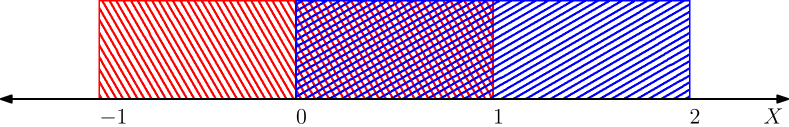
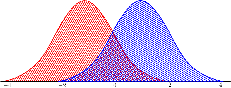
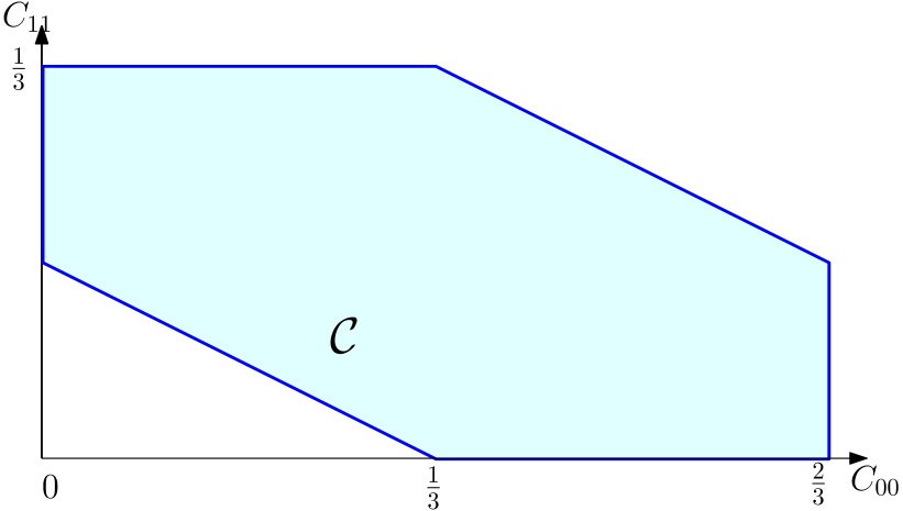
(a) Unif: $X|Y=0$ and $X|Y=1$ are uniform distributions over $[-1,1]$ and $[0,2]$ respectively; $P(Y=1)=\frac{1}{3}$.

(b) NormBal: $X|Y=0$ and $X|Y=1$ are Gaussians with means $-\frac{1}{2}$ and $\frac{1}{2}$ respectively; $P(Y=1)=\frac{1}{2}$.

(c) NormImbal: $X|Y=0$ and $X|Y=1$ are Gaussians with means $-\frac{1}{2}$ and $\frac{1}{2}$ respectively; $P(Y=1)=\frac{1}{5}$.

Figure 2: The set of achievable confusion matrices ${\mathcal{C}}$ for three example binary-labeled distributions: (a) Unif, (b) NormBal, and (c) NormImbal. The top row figures show the class-conditional distributions, and the bottom row figures represent the corresponding ${\mathcal{C}}$. While the confusion matrix has four entries, there are only two degrees of freedom (the rows of the confusion matrix sum to the prior probabilities). We therefore only illustrate the projection of ${\mathcal{C}}$ on to the diagonal entries $C_{00}$ and $C_{11}$. Note that the scales in the bottom row figures are different.

In order to understand optimal classifiers for the more complex learning problems in OP1 and OP2 described in the previous section, we will find it useful to view these learning problems as optimization problems over all achievable confusion matrices:

Definition 6 (Achievable confusion matrices).

Define the set of achievable confusion matrices w.r.t. $D$ as the set of all confusion matrices achieved by some randomized classifier:

$${\mathcal{C}}=\big{\{}\textrm{{vec}}({\mathbf{C}}[h])\,|\,~{}h:{\mathcal{X}}{\rightarrow}\Delta_{n}\big{\}}\subseteq\Delta_{d}$$

where $\textrm{{vec}}({\mathbf{C}}[h])\,=\,\left[C_{11}[h],\ldots,C_{1n}[h],\ldots,C_{n1}[h],\ldots,C_{nn}[h]\right]$ is of dimension $d=n^{2}$.

See Figure 2 for an illustration of the set of achievable confusion matrices for three simple synthetic distributions, which we will refer to as Unif, NormBal and NormImBal. For ease of exposition, in the above definition, we represent the achievable confusion matrices by a set of flattened vectors of dimension $d=n^{2}$. We will also find it convenient from now on to overload notation and denote the performance measures by a function $\psi:[0,1]^{d}{\rightarrow}{\mathbb{R}}_{+}$ mapping a $d$-dimensional vector representation of the confusion matrix to a non-negative real number, and the constraints by functions $\phi_{1},\ldots,\phi_{K}:[0,1]^{d}{\rightarrow}{\mathbb{R}}_{+}$ defined on $d$-dimensional vectors. We will similarly represent an $n\times n$ loss matrix by a flattened $d$-dimensional vector ${\mathbf{L}}\in{\mathbb{R}}^{d}$.

Proposition 7.

${\mathcal{C}}$ is a convex set.

Proof. For any ${\mathbf{C}}_{1},{\mathbf{C}}_{2}\in{\mathcal{C}}$ and $\gamma\in[0,1]$, we will show $\gamma{\mathbf{C}}_{1}+(1-\gamma){\mathbf{C}}_{2}\in{\mathcal{C}}$. Clearly, there exists randomized classifiers $h_{1},h_{2}:{\mathcal{X}}{\rightarrow}\Delta_{n}$ such that ${\mathbf{C}}_{1}={\mathbf{C}}[h_{1}]$ and ${\mathbf{C}}_{2}={\mathbf{C}}[h_{2}]$. Since $h(x)=\gamma h_{1}(x)+(1-\gamma)h_{2}(x)$ is a valid randomized classifier, ${\mathbf{C}}[h]=\gamma{\mathbf{C}}_{1}+(1-\gamma){\mathbf{C}}_{2}\in{\mathcal{C}}.$ ∎

The set ${\mathcal{C}}$ will play an important role in both our analysis of optimal classifiers and the subsequent development of consistent algorithms. Clearly, we can write OP1 as an unconstrained $d$-dimensional optimization problem over the convex set ${\mathcal{C}}$:

$$\min_{h:{\mathcal{X}}{\rightarrow}\Delta_{n}}\Psi[h] =\min_{{\mathbf{C}}\in{\mathcal{C}}}\psi({\mathbf{C}}),$$ (OP1*)

and write OP2 as a constrained optimization problem over ${\mathcal{C}}$:

$$\min_{h:{\mathcal{X}}{\rightarrow}\Delta_{n},\Phi_{k}[h]\leq 0,\forall k}\Psi[h] =\min_{{\mathbf{C}}\in{\mathcal{C}},{\boldsymbol{\phi}}({\mathbf{C}})\leq{\mathbf{0}}}\psi({\mathbf{C}}),$$ (OP2*)

where we denote $\boldsymbol{\phi}({\mathbf{C}})\,=\,[\phi_{1}({\mathbf{C}}),\ldots,\phi_{K}({\mathbf{C}})]$.

3.1 Bayes Optimal Classifier for the Unconstrained Problem

While it is not clear if a classifier achieving the Bayes optimal performance exists in general, we show below that under mild assumptions, the optimal classifier for the unconstrained problem in OP1 can always be expressed as the optimal classifier for a certain linear performance metric. We show this for “ratio-of-linear” performance measures $\psi$, and for “monotonic” performance measures $\psi$ under a mild continuity assumption on $D$.

Proposition 8 (Bayes optimal classifier for ratio-of-linear $\psi$).

Let the performance measure $\psi:[0,1]^{d}{\rightarrow}{\mathbb{R}}_{+}$ in OP1 be of the form $\psi({\mathbf{C}})=\frac{\langle{\mathbf{A}},{\mathbf{C}}\rangle}{\langle{\mathbf{B}},{\mathbf{C}}\rangle}$ for some ${\mathbf{A}},{\mathbf{B}}\in{\mathbb{R}}^{d}$ with $\langle{\mathbf{B}},{\mathbf{C}}\rangle>0~{}\forall{\mathbf{C}}\in{\mathcal{C}}$. Then there exists loss matrix ${\mathbf{L}}^{*}$ (which depends on $\psi$ and $D$) such that any classifier that is optimal for the linear metric $\langle{\mathbf{L}}^{*},{\mathbf{C}}\rangle$ is also optimal for OP1.

Proposition 9 (Bayes optimal classifier for monotonic $\psi$).

Let $\psi:[0,1]^{d}{\rightarrow}{\mathbb{R}}_{+}$ in OP1 be differentiable and bounded, and be monotonically decreasing in $C_{ii}$ for each $i$ and non-decreasing in $C_{ij}$ for all $i,j$. Assume ${{\boldsymbol{\eta}}}(X)$ is a continuous random vector. Then there exists a loss matrix ${\mathbf{L}}^{*}$ (which depends on $\psi$ and $D$) such that any classifier that is optimal for the linear metric $\langle{\mathbf{L}}^{*},{\mathbf{C}}\rangle$ over ${\mathcal{C}}$ is also optimal for OP1.

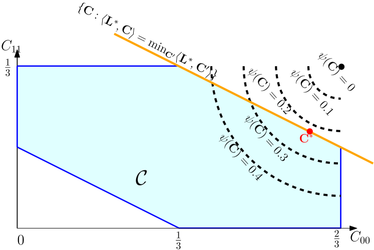
(a)

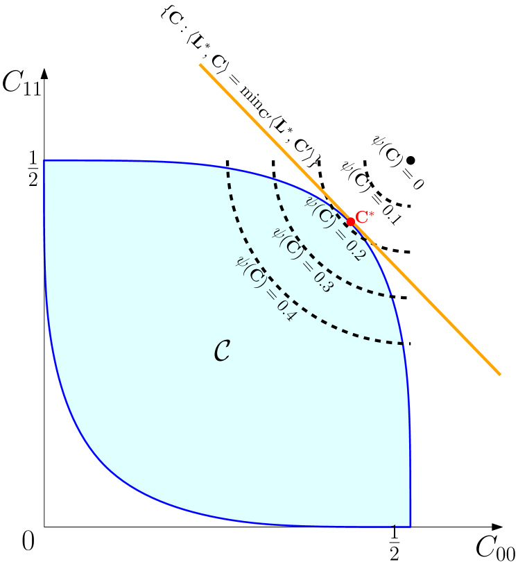
(b)

Figure 3: Illustration of the Bayes-optimal classifier for the unconstrained problem in OP1 with a monotonic $\psi$. The figures show the set of confusion matrices ${\mathcal{C}}$ for distributions Unif (left) and NormBal (right) in Figure 2 (represented by the diagonal entries), the contours of the monotonic performance metric $\psi$, and the corresponding solution ${\mathbf{C}}^{*}$ to $\min_{{\mathbf{C}}\in{\mathcal{C}}}\psi({\mathbf{C}})$ (red dot). The black dot denotes the minimizer over all confusion matrices (even those that are not achievable).

See Appendices A.1 and A.2 for the proofs. In Figure 3, we provide an illustration for Proposition 9 using the 2-class example distributions Unif and NormBal from Figure 2. We consider a monotonic performance metric $\psi$ whose contours are shown overlayed in the figure with the set of feasible confusion matrices ${\mathcal{C}}$. It can be clearly seen that the minimal value of $\psi$ over ${\mathcal{C}}$ is achieved by a point ${\mathbf{C}}^{*}$ on the boundary. Because ${\mathcal{C}}$ is a convex set, it follows that all points on the boundary of ${\mathcal{C}}$ are minimizers of some linear function $\langle{\mathbf{L}},{\mathbf{C}}\rangle$ over ${\mathbf{C}}\in{\mathcal{C}}$. Therefore, ${\mathbf{C}}^{*}$ is also a minimizer of $\langle{\mathbf{L}}^{*},{\mathbf{C}}\rangle$ for some loss matrix ${\mathbf{L}}^{*}$.

However, for ${\mathbf{C}}^{*}$ to be a unique minimizer of $\langle{\mathbf{L}}^{*},{\mathbf{C}}\rangle$, we need the additional continuity assumption on ${\boldsymbol{\eta}}(X)$ in Proposition 9 to hold. This does not hold for the Unif distribution in Figure 2(a), where the corresponding conditional-class probability vectors ${\boldsymbol{\eta}}(X)$ take only 3 possible values in $\Delta_{2}$. In contrast, ${\boldsymbol{\eta}}(X)$ is continuous for the NormBal distribution in Figure 3(b), and as result, the minimizer ${\mathbf{C}}^{*}$ of $\psi({\mathbf{C}})$, is also a unique minimizer for some linear function $\langle{\mathbf{L}}^{*},{\mathbf{C}}\rangle$.

In Figure 4, we compare the forms of the Bayes-optimal classifier for the standard 0-1 loss and for the H-mean loss in Table 1. The latter seeks to explicitly balance the classifier’s performance across all classes and is a monotonic function of (the diagonal elements of) ${\mathbf{C}}$. We provide plots of the optimal classifiers for a toy 3-class distribution, which contains equal class priors and has a conditional-class probability distribution ${\boldsymbol{\eta}}(X)$ which is continuous. We know that the optimal classifier for the 0-1 loss simply outputs the label with the maximum class probability $h^{*}(x)=\operatorname{argmax}^{*}_{i}\eta_{i}(x)$. As seen in Figure 4(a), despite the class priors being equal, this classifier predicts class 1 on only a small fraction of instances. On the other hand, for the H-mean loss, Proposition 9 tells us that the optimal classifier can be obtained by minimizing some linear function of ${\mathbf{C}}$, the optimal classifier for which, in this particular case, is of the form $h^{*}(x)=\operatorname{argmax}^{*}_{i}w^{*}_{i}\eta_{i}(x)$, for some distribution-dependent weights $w^{*}_{i}\in{\mathbb{R}}_{+}$. Note that $w^{*}_{i}$ can be seen as the penalty associated with a wrong prediction on class $i$, which in this case is the highest for class 1. The resulting classifier, shown in Figure 4(b), therefore yields equitable performance across the three classes.

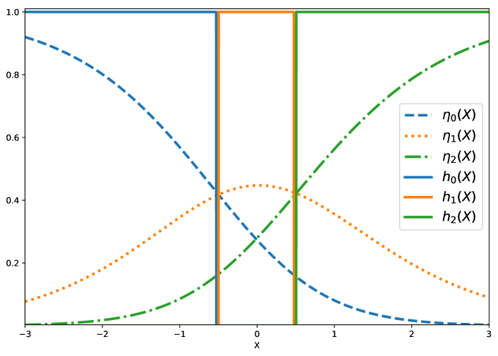
(a) Bayes-optimal classifier for 0-1 loss

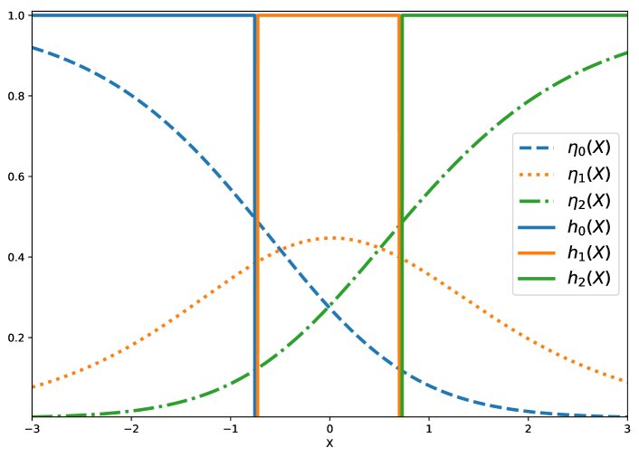
(b) Bayes-optimal classifier for H-mean loss

Figure 4: Comparison of Bayes-optimal classifiers for the 0-1 loss (left) and the H-mean loss (right). We use a toy 3-class (denoted as class 0, 1 and 2) distribution over an one-dimensional instance space ${\mathcal{X}}={\mathbb{R}}$, with equal priors, and with the class-conditional distribution for the three classes being a Gaussian distribution with means $-1,0$ and $1$ respectively and variance 1. We plot the conditional-class probability function $\eta_{i}(X)$, and the outputs of the optimal classifier $h^{*}_{i}(X)$ for each class $i\in[3]$. For the 0-1 loss, the optimal classifier predicts class 1 only on a small fraction of examples, whereas for the optimal classifier H-mean loss has greater coverage for class 1.

3.2 Bayes Optimal Classifier for the Constrained Problem

In both the characterizations in the previous section, the Bayes-optimal classifier for the unconstrained problem in OP1 is deterministic. An analogous statement does not hold in general for the constrained problem in OP2. However, we can prove a weaker characterization for OP2 showing that the Bayes optimal classifier is a randomized classifier that is supported by at most $d+1$ deterministic classifiers.

Proposition 10 (Bayes optimal classifier for continuous $\psi,\phi_{1},\ldots,\phi_{K}$).

Let the performance measure $\psi:[0,1]^{d}{\rightarrow}{\mathbb{R}}_{+}$ and the constraint functions $\phi_{1},\ldots,\phi_{K}:[-1,1]^{d}{\rightarrow}{\mathbb{R}}_{+}$ in OP2 be continuous and bounded. Then there exists $d+1$ loss matrices ${\mathbf{L}}^{*}_{1},{\mathbf{L}}^{*}_{2},\ldots,{\mathbf{L}}^{*}_{d+1}$ (which can depend on $\psi,\phi_{k}$’s and $D$) such that an optimal classifier for OP2 can be expressed as a randomized combination of the deterministic classifiers $h_{1},h_{2},\ldots,h_{d+1}$, where $h_{i}$ is optimal for the linear metric given by ${\mathbf{L}}^{*}_{i}$.

See Appendix A.3 for the proof. When the objective and constraints $\psi,\phi_{1},\ldots,\phi_{K}$ together depend on fewer than $d=n^{2}$ entries of the confusion matrix, we can extend the above proposition to show that the number of deterministic classifiers needed to construct an optimal classifier for OP2 is at most one plus the number of confusion matrix entries the metrics depend on. For example, if we wish to optimize the G-mean metric (Example 3) subject to a constraint on the class-1 precision (Example 5), the objective and constraints together depend only on $2n-1$ “entries” of the confusion matrix, and so an optimal classifier for this problem can be expressed as randomized combination of at most $2n$ deterministic classifiers. In Section 7, we provide a more detailed discussion about succinct vector representations for confusion matrices that require fewer than $n^{2}$ entries.

Under continuity assumptions on ${\boldsymbol{\eta}}(X)$ (which essentially translate to the space of achievable confusion matrices ${\mathcal{C}}$ being strictly convex), one can further show that the Bayes-optimal classifier can be expressed as a randomized combination of two deterministic classifiers $h_{1}$ and $h_{2}$, where $h_{i}$ is optimal for some linear metric ${\mathbf{L}}^{*}_{i}$ (Yang et al., 2020). The same characterization straight-forwardly holds for unconstrained minimization of a general performance metric $\psi$ (Wang et al., 2019).

3.3 Naïve Plug-in Approach

The characterization results for the unconstrained problem in OP1 suggest a simple algorithmic approach to finding the optimal classifier: search over a large range of loss matrices ${\mathbf{L}}$, estimate the optimal classifier for each such ${\mathbf{L}}$, and select among these a classifier that yields maximal $\psi$-performance (e.g. on a held-out validation data set). This is the analogue of “plug-in” type methods for binary performance metrics (such as those considered by Koyejo et al. (2014) and Narasimhan et al. (2014)), where one searches over possible thresholds on the (estimated) class probability function. However, while the binary case involves a search over values for a single threshold parameter, in the multiclass case, one may need to perform a brute-force search over as many as $d$ parameters, requiring time exponential in $d$. For large $d$, such a naïve plug-in approach is computationally intractable. In fact, this procedure becomes even more difficult to implement for the constrained problem in OP2, where the optimal classifier is a randomized combination of multiple ${\mathbf{L}}$-optimal classifiers, requiring a brute-force search of over multiple loss matrices ${\mathbf{L}}$.

In what follows, we will design efficient learning algorithms that instead search over the space of feasible confusion matrices ${\mathcal{C}}$ using suitable optimization methods.

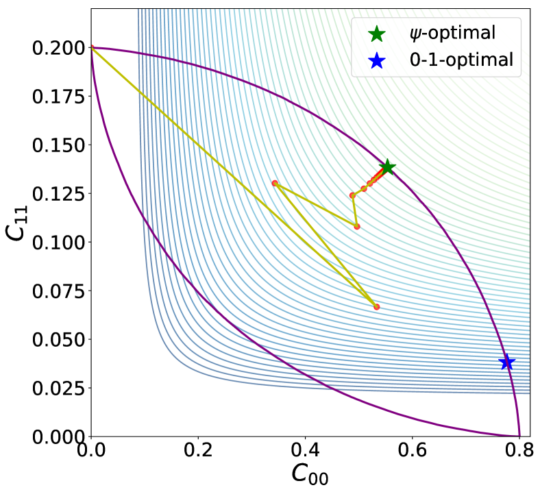
(a) Frank-Wolfe

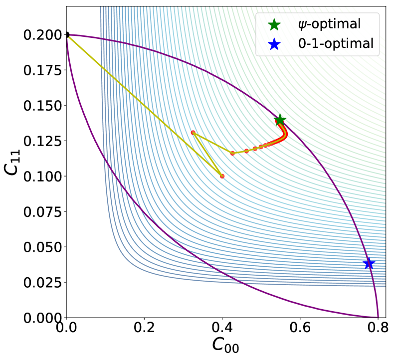
(b) GDA

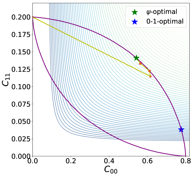
(c) Ellipsoid

Figure 5: Illustration of the Frank-Wolfe (Algorithm 1), Gradient Descent-Ascent (Algorithm 2) and Ellipsoid (Algorithm 3) algorithms in minimizing the H-mean loss $\psi^{\textup{{HM}}}$ on the NormImbal distribution in Figure 2(c). The figures contain the space of achievable confusion matrices ${\mathcal{C}}$ (with purple colored boundary), along with the contours of $\psi^{\textup{{HM}}}$. The trajectory of the confusion matrix ${\mathbf{C}}[\bar{h}^{t}]$ of the averaged classifier up until iteration $t$ is shown, where $\bar{h}^{t}=h^{t}$ for Frank-Wolfe, $\bar{h}^{t}=\frac{1}{t}\sum_{\tau=1}^{\tau}h^{t}$ for GDA, and $\bar{h}^{t}=\frac{1}{t}\sum_{\tau=1}^{t}\alpha^{*}_{\tau}h^{\tau}$ for ellipsoid, with the optimal coefficients ${\boldsymbol{\alpha}}^{*}\in\operatorname{argmin}_{{\boldsymbol{\alpha}}\in\Delta_{t}}\psi\left(\sum_{\tau=1}^{t}\alpha_{\tau}{\mathbf{C}}^{\tau}\right)$ computed for iterates $1,\ldots t$. The averaged classifier is seen to converge to an optimal classifier for the H-mean loss and away from that for the 0-1 loss.

Table 2: Algorithms for the unconstrained problem in OP1, with the number calls to the LMO and the optimality gap $\psi({\mathbf{C}}[\bar{h}])-\min_{{\mathbf{C}}\in{\mathcal{C}}}\psi({\mathbf{C}})$ for the returned classifier $\bar{h}$. Here $\rho^{\textup{{eff}}}=\rho+\sqrt{d}\rho^{\prime}$.

Algorithm	Assumption on $\psi$	# LMO Calls	Optimality Gap
Frank-Wolfe	Convex, smooth, Lipschitz	$\displaystyle{\mathcal{O}}\left(1/\epsilon\right)$	${\mathcal{O}}\big{(}\epsilon+\rho^{\textup{{eff}}}\big{)}$
Gradient Descent-Ascent	Convex, Lipschitz	$\displaystyle{\mathcal{O}}\left(1/\epsilon^{2}\right)$	${\mathcal{O}}\big{(}\epsilon+\rho^{\textup{{eff}}}\big{)}$
Ellipsoid	Convex, Lipschitz	$\displaystyle{\mathcal{O}}\left(d^{2}\log(d/\epsilon)\right)$	${\mathcal{O}}(\epsilon+\rho^{\textup{{eff}}})$
Bisection	Ratio-of-linear	$\displaystyle{\mathcal{O}}\left(\log(1/\epsilon)\right)$	${\mathcal{O}}\left(\epsilon+\rho^{\textup{{eff}}}\right)$

4 Algorithms for Unconstrained Problems

We start with algorithms for solving the unconstrained learning problem in OP1. As a running example to illustrate our algorithms, we will use the task of maximizing the H-mean loss on the NormImbal distribution described in Figure 2(e).

As noted in our discussion of OP1*, one can view OP1 as an optimization problem over ${\mathcal{C}}$: $\min_{{\mathbf{C}}\in{\mathcal{C}}}\psi({\mathbf{C}})$. While ${\mathcal{C}}$ is a convex set, it is not available directly to the learner as the set of all confusion matrices is hard to characterize. On the other hand, one operation that is easy to perform is to find an optimal classifier for a linear loss $\langle{\mathbf{L}},{\mathbf{C}}\rangle$ over ${\mathcal{C}}$. Indeed this amounts to solving a cost-sensitive learning problem (Elkan, 2001), a task for which there are numerous classical methods available. So we assume access to an oracle for solving this linear minimization problem over ${\mathcal{C}}$, which takes as input a loss matrix ${\mathbf{L}}$ and a sample $S$, and outputs a classifier $\widehat{g}$ and an estimate of the confusion matrix at $\widehat{g}$ with the following properties:

Definition 11 (Linear minimization oracle).

Let $\rho,\rho^{\prime},\delta\in(0,1)$. A linear minimization oracle, denoted by $\Omega$, takes a loss matrix ${\mathbf{L}}\in{\mathbb{R}}^{d}$ and a sample $S$ as input, and outputs a classifier $\widehat{g}$ and a confusion matrix $\widehat{{\boldsymbol{\Gamma}}}\in{\mathbb{R}}^{d}$. We say $\Omega$ is a $(\rho,\rho^{\prime},\delta)$-approximate LMO for sample size $N$, if, with probability $\geq 1-\delta$ over draw of $S\sim D^{N}$, for any ${\mathbf{L}}\in{\mathbb{R}}_{+}^{d}$ with $\|{\mathbf{L}}\|_{\infty}\leq 1$, it outputs $(\widehat{g},\widehat{{\boldsymbol{\Gamma}}})=\Omega({\mathbf{L}};S)$ such that:

$$\langle{\mathbf{L}},{\mathbf{C}}[\widehat{g}]\rangle\,\leq\,\min_{h:{\mathcal{X}}{\rightarrow}\Delta_{n}}\langle{\mathbf{L}},{\mathbf{C}}[h]\rangle+\rho;\quad\|{\mathbf{C}}[\widehat{g}]\,-\,\widehat{{\boldsymbol{\Gamma}}}\|_{\infty}\,\leq\,\rho^{\prime}.$$

The approximation constants $\rho$ and $\rho^{\prime}$ may in turn depend on the sample size $N$, the dimension $d$ and the confidence level $\delta$.

In Section 6, we discuss a practical plug-in based algorithm for implementing an LMO with these approximation properties. Equipped with access to such an LMO, we develop algorithms based on iterative optimization methods for minimizing $\psi$ over ${\mathcal{C}}$. Our algorithms do not require direct access to the set ${\mathcal{C}}$, but only make use of calls to the LMO over ${\mathcal{C}}$.

We present four algorithms under different assumptions on the metric $\psi$ and show convergence guarantees in each case (see Table 2 for a summary of our results). The proofs build on existing techniques for showing convergence of the respective optimization solvers, and need to additionally take into account the errors in the LMO calls.

Algorithm 1 Frank-Wolfe (FW) Algorithm for OP1 with Smooth Convex $\psi$

1:  Input: $\psi:[0,1]^{d}\to[0,1]$, an LMO $\Omega$, $S=\{(x_{1},y_{1}),\ldots,(x_{N},y_{N})\}$, $T$

2:  Initialize: $(h^{0},{\mathbf{C}}^{0})=\Omega({\mathbf{L}}^{0};S)$ for an arbitrary loss matrix ${\mathbf{L}}^{0}$

3:  For $t=1$ to $T$ do

4:       ${\mathbf{L}}^{t}\,=\,\frac{\nabla\psi({\mathbf{C}}^{t-1})}{\|\nabla\psi({\mathbf{C}}^{t-1})\|_{\infty}}$

5:       $(\widetilde{h}^{t},\widetilde{{\mathbf{C}}}^{t})\,=\,\Omega({\mathbf{L}}^{t};S)$

6:       ${h}^{t}=\big{(}1-\frac{2}{t+1}\big{)}{h}^{t-1}+\frac{2}{t+1}\widetilde{h}^{t}$

7:       ${{\mathbf{C}}}^{t}=\big{(}1-\frac{2}{t+1}\big{)}{{\mathbf{C}}}^{t-1}+\frac{2}{t+1}\widetilde{{\mathbf{C}}}^{t}$

8:  End For

9:  Output: $\bar{h}=h^{T}$

4.1 Frank-Wolfe Algorithm for Smooth Convex Metrics

The first algorithm that we describe uses the classical Frank-Wolfe method (Frank and Wolfe, 1956) to minimize $\psi({\mathbf{C}})$ over ${\mathbf{C}}$ for performance measures $\psi$ that are convex and smooth over ${\mathcal{C}}$. Examples of performance measures with these properties include the H-mean and Q-mean in Table 1.

The key idea behind this algorithm is to sequentially linearize the objective $\psi$ using its local gradients, and minimize the linear approximation over ${\mathcal{C}}$ using the LMO. The procedure, outlined in Algorithm 1, maintains iterates of confusion matrices ${\mathbf{C}}^{t}$, computes the gradient ${\mathbf{L}}^{t}=\nabla\psi({\mathbf{C}}^{t-1})$ for the current iterate, invokes the LMO to solve the resulting linear minimization problem $\min_{{\mathbf{C}}\in{\mathcal{C}}_{D}}\langle{\mathbf{L}}^{t},{\mathbf{C}}\rangle$, and updates ${\mathbf{C}}^{t}$ based on the result of the linear minimization. The minimizer ${\mathbf{C}}^{*}$ of $\psi({\mathbf{C}})$ can then be approximated by a combination of the iterates ${\mathbf{C}}^{1},\ldots,{\mathbf{C}}^{T}$, with the final classifier that achieves this confusion matrix given by a randomized combination of classifiers learned across all the iterations.

For metrics $\psi$ that are smooth, we show that the algorithm takes ${\mathcal{O}}(1/\epsilon)$ calls to the LMO to reach a classifier that is ${\mathcal{O}}(\epsilon+c)$-optimal for a constant $c>0$ that depends on the LMO error.

Theorem 12 (Convergence of FW algorithm).

Fix $\epsilon\in(0,1)$. Let $\psi:[0,1]^{d}{\rightarrow}[0,1]$ be convex, $\beta$-smooth and $L$-Lipschitz w.r.t. the $\ell_{2}$-norm. Let $\Omega$ in Algorithm 1 be a $(\rho,\rho^{\prime},\delta)$-approximate LMO for sample size $m$. Let $\bar{h}$ be a classifier returned by Algorithm 1 when run for $T$ iterations. Then with probability $\geq 1-\delta$ over draw of $S\sim D^{N}$, after $T={\mathcal{O}}(1/\epsilon)$ iterations:

$$\psi({\mathbf{C}}[\bar{h}])\,\leq\,\min_{{\mathbf{C}}\in{\mathcal{C}}}\,\psi({\mathbf{C}})+8\beta\epsilon+2L\rho+4\beta\sqrt{d}\rho^{\prime}\leq\min_{{\mathbf{C}}\in{\mathcal{C}}}\,\psi({\mathbf{C}})+{\mathcal{O}}(\epsilon+\rho^{\textup{{eff}}}),$$

where $\rho^{\textup{{eff}}}=\rho+\sqrt{d}\rho^{\prime}$.

Proof.

See Appendix A.4. ∎

The proof derives a version of the convergence guarantee for the Frank-Wolfe method (Jaggi, 2013) which is robust to errors in the gradients and confusion matrix estimates.

In Figure 5(a), we illustrate the trajectory taken by the Frank-Wolfe algorithm in minimizing the H-mean loss $\psi^{\textup{{HM}}}$ in Table 1. Notice that the linear minimization outputs $\widetilde{{\mathbf{C}}}^{t}$ lie on the boundary of ${\mathcal{C}}$, while the averaged confusion matrix iterates ${\mathbf{C}}^{t}$ lie in the interior. Also note that because NormImbal distribution we use for this illustration has significant class imbalance, the minimizer for the 0-1 loss incurs a large H-mean loss. In contrast, Algorithm 1 converges to a confusion matrix with substantially better H-mean loss.

4.2 Gradient Descent-Ascent Algorithm for Non-smooth Convex Metrics

The next algorithm we propose is designed for performance measures $\psi$ that are convex, but not necessarily smooth, such as the min-max metric in Table 1. We make use of the “three player” framework proposed by Narasimhan et al. (2019) and provide a slight variant of the “oracle-based algorithm” in their paper.

As a first step, we decouple the confusion matrix ${\mathbf{C}}$ from the function $\psi$ in OP1* by introducing auxiliary slack variables ${\boldsymbol{\xi}}\in\Delta_{d}$, and arrive at the following equivalent problem:

$$\min_{{\mathbf{C}}\in{\mathcal{C}}}\psi({\mathbf{C}}) =\min_{{\mathbf{C}}\in{\mathcal{C}},\,{\boldsymbol{\xi}}\in\Delta_{d},\,{\boldsymbol{\xi}}={\mathbf{C}}}\psi({\boldsymbol{\xi}}),$$ (1)

where we constraint the slack variables $\xi$ to be equal to the confusion matrix ${\mathbf{C}}$. We define the Lagrangian for the above problem introducing multipliers $\boldsymbol{\lambda}\in{\mathbb{R}}^{d}$ for the $d$ equality constraints:

$$\mathcal{L}({\mathbf{C}},{\boldsymbol{\xi}},\boldsymbol{\lambda}) =\psi({\boldsymbol{\xi}})+\langle\boldsymbol{\lambda},{\mathbf{C}}-{\boldsymbol{\xi}}\rangle,$$ (2)

and re-formulate (1) as an equivalent min-max problem where we minimize the Lagrangian over ${\boldsymbol{\xi}}$ and ${\mathbf{C}}$, and maximize it over the Lagrange multipliers $\boldsymbol{\lambda}$:

$$\min_{{\mathbf{C}}\in{\mathcal{C}}}\psi({\mathbf{C}}) =\min_{{\mathbf{C}}\in{\mathcal{C}},\,{\boldsymbol{\xi}}\in[0,1]^{d}}\,\max_{\boldsymbol{\lambda}\in{\mathbb{R}}^{d}}\,\mathcal{L}({\mathbf{C}},{\boldsymbol{\xi}},\boldsymbol{\lambda}).$$ (3)

The minimizer of $\psi({\mathbf{C}})$ over ${\mathbf{C}}$ can be then obtained by finding a saddle point of the above min-max problem. To this end, we first notice that the Lagrangian $\mathcal{L}$ is linear in ${\mathbf{C}}$, convex in ${\boldsymbol{\xi}}$ and linear in $\boldsymbol{\lambda}$. Following Narasimhan et al. (2019), we maintain iterates ${\mathbf{C}}^{t},{\boldsymbol{\xi}}^{t}$ and $\boldsymbol{\lambda}^{t}$ and at each iteration, perform a full minimization of $\mathcal{L}$ using a call to the LMO, perform gradient descent updates on ${\boldsymbol{\xi}}$, and perform gradient ascent updates on $\boldsymbol{\lambda}$. We constrain ${\boldsymbol{\xi}}$ to be within the probability simplex $\Delta_{d}$, and for technical reasons, also constrain $\boldsymbol{\lambda}$ to be within a bounded set $\Lambda$, both of which are accomplished using projection operations.

The resulting gradient descent-ascent procedure, outlined in Algorithm 2 can be shown to converge to an approximate saddle point of (3). In fact, one can further show that with ${\mathcal{O}}(\log(d)/\epsilon^{2})$ calls to the LMO, the algorithm finds a classifier that is ${\mathcal{O}}(\epsilon+c)$-optimal for $\psi$, for some constant $c>0$ that depends on the LMO errors:

Theorem 13 (Convergence of GDA algorithm).

Fix $\epsilon\in(0,1)$. Let $\psi:[0,1]^{d}{\rightarrow}[0,1]$ be convex and $L$-Lipschitz w.r.t. the $\ell_{2}$-norm. Let $\Omega$ in Algorithm 2 be a $(\rho,\rho^{\prime},\delta)$-approximate LMO for sample size $N$. Let the space of Lagrange multipliers $\Lambda=\{\boldsymbol{\lambda}\in{\mathbb{R}}^{d}\,|\,\|\boldsymbol{\lambda}\|_{2}\leq 2L\}$. Let $\bar{h}$ be a classifier returned by Algorithm 2 when run for $T$ iterations, with step-sizes $\eta=\frac{1}{4L\sqrt{2T}}$ and $\eta^{\prime}=\frac{4L}{\sqrt{2T}}$. Then with probability $\geq 1-\delta$ over draw of $S\sim D^{N}$, after $T={\mathcal{O}}(1/\epsilon^{2})$ iterations:

$$\psi({\mathbf{C}}[\bar{h}])\,\leq\,\min_{{\mathbf{C}}\in{\mathcal{C}}}\,\psi({\mathbf{C}})\,+\,{\mathcal{O}}\left(\epsilon+\rho^{\textup{{eff}}}\right),$$

where $\rho^{\textup{{eff}}}=\rho+\sqrt{d}\rho^{\prime}$ and ${\mathcal{O}}$ hides constants independent of $\epsilon,\rho,\rho^{\prime}$ and $d$.

Proof.

See Appendix A.5. ∎

Figure 5(b) shows the trajectory of the iterates of the GDA algorithm on the same running example used to illustrate the Frank-Wolfe based algorithm. Notice that the GDA algorithm converges to an optimal confusion matrix (classifier) for the problem.

Algorithm 2 Gradient Descent-Ascent (GDA) Algorithm for OP1 with Non-smooth Convex $\psi$

1:  Input: $\psi:[0,1]^{d}\to[0,1]$, an LMO $\Omega$ , $S=\{(x_{1},y_{1}),\ldots,(x_{N},y_{N})\}$, $T$, space of Lagrange multipliers $\Lambda\subset{\mathbb{R}}^{d}$

2:  Parameters: Step-sizes $\eta,\eta^{\prime}>0$

3:  Initialize: $\boldsymbol{\lambda}^{0}\in\Lambda$

4:  For $t=0$ to $T-1$ do

5:       ${\mathbf{L}}^{t}\,=\,\frac{\boldsymbol{\lambda}^{t}}{\|\boldsymbol{\lambda}^{t}\|_{\infty}}$

6:       $(h^{t},{\mathbf{C}}^{t})\,=\,\Omega({\mathbf{L}}^{t};S)$

7:       $\widetilde{{\boldsymbol{\xi}}}\,=\,{\boldsymbol{\xi}}^{t}\,-\,\eta\nabla_{{\boldsymbol{\xi}}}\mathcal{L}({\mathbf{C}}^{t},{\boldsymbol{\xi}}^{t},\boldsymbol{\lambda}^{t});$      ${\boldsymbol{\xi}}^{t+1}\,\in\,\operatorname{argmin}_{{\boldsymbol{\xi}}\in\Delta_{d}}\,\|{\boldsymbol{\xi}}-\widetilde{{\boldsymbol{\xi}}}\|_{2}$

8:       $\widetilde{\boldsymbol{\lambda}}\,=\,\boldsymbol{\lambda}^{t}\,+\,\eta^{\prime}\nabla_{\boldsymbol{\lambda}}\mathcal{L}({\mathbf{C}}^{t},{\boldsymbol{\xi}}^{t},\boldsymbol{\lambda}^{t});$      $\boldsymbol{\lambda}^{t+1}\,\in\,\operatorname{argmin}_{\boldsymbol{\lambda}\in\Lambda}\|\boldsymbol{\lambda}-\widetilde{\boldsymbol{\lambda}}\|_{2}$

9:  End For

10:  Output: $\bar{h}=\frac{1}{T}\sum_{t=1}^{T}h^{t}$

4.3 Ellipsoid Algorithm for Non-smooth Convex Metrics

Algorithm 3 Ellipsoid Algorithm for OP1 with Non-smooth Convex $\psi$

1:  Input: $\psi:[0,1]^{d}\to[0,1]$, an LMO $\Omega$, $S=\{(x_{1},y_{1}),\ldots,(x_{m},y_{m})\},T$

2:  Parameters: Initial ellipsoid radius $a$

3:  Initialize: $\widetilde{\boldsymbol{\lambda}}^{0}={\mathbf{0}}_{d}$, $\widetilde{{\mathbf{A}}}^{0}=a^{2}{\mathbf{I}}_{d}$

4:  For $t=0$ to $T-1$ do

5:       If $\|\widetilde{\boldsymbol{\lambda}}^{t}\|_{2}>a:$

6:           ${\mathbf{A}}^{t+1},\boldsymbol{\lambda}^{t+1}=\text{JLE}({{\mathbf{A}}}^{t},{\boldsymbol{\lambda}}^{t},-{\boldsymbol{\lambda}}^{t})$

7:           $h^{t},{\mathbf{C}}^{t}=h^{0},{\mathbf{C}}^{0}$; continue

8:       Else:

9:           ${\mathbf{A}}^{t},\boldsymbol{\lambda}^{t}=\widetilde{{\mathbf{A}}}^{t},\widetilde{\boldsymbol{\lambda}}^{t}$

10:           $(h^{t},{\mathbf{C}}^{t})=\Omega(\boldsymbol{\lambda}^{t},S)$

11:           ${\boldsymbol{\xi}}^{t}=\operatorname{argmin}_{{\boldsymbol{\xi}}\in\Delta_{d}}\psi({\boldsymbol{\xi}})-\langle\boldsymbol{\lambda}^{t},{\boldsymbol{\xi}}\rangle$

12:           ${\mathbf{A}}^{t+1},\boldsymbol{\lambda}^{t+1}=\text{JLE}({\mathbf{A}}^{t},\boldsymbol{\lambda}^{t},{\mathbf{C}}^{t}-{\boldsymbol{\xi}}^{t})$

13:  End For

14:  ${\boldsymbol{\alpha}}^{*}\in\operatorname{argmin}_{{\boldsymbol{\alpha}}\in\Delta_{T}}\psi\left(\sum_{t=0}^{T-1}\alpha_{t}{\mathbf{C}}^{t}\right)$

15:  Ouput: $\bar{h}=\sum_{t=0}^{T-1}\alpha^{*}_{t}h^{t}$

Algorithm 3(a) John-Lowner Ellipsoid (JLE) Construction

1:  Input: Positive-definite matrix ${\mathbf{A}}\in{\mathbb{R}}^{d\times d}$, $\boldsymbol{\lambda}$, $\mathbf{w}$

2:  Output: ${\mathbf{A}}^{\prime},\boldsymbol{\lambda}^{\prime}$ that parameterizes the smallest ellipsoid such that:

$$E(\boldsymbol{\lambda}^{\prime},{\mathbf{A}}^{\prime})\supseteq E(\boldsymbol{\lambda},{\mathbf{A}})\cap\{{\mathbf{x}}:({\mathbf{x}}-\boldsymbol{\lambda})^{\top}\mathbf{w}\geq 0\}$$

where $E(\boldsymbol{\lambda},{\mathbf{A}})=\{{\mathbf{x}}:({\mathbf{x}}-\boldsymbol{\lambda})^{\top}({\mathbf{A}})^{-1}({\mathbf{x}}-\boldsymbol{\lambda})\leq 1\}$

3:  $t=\frac{1}{d+1},a=\frac{1}{(1-t)^{2}},b=\frac{1-2t}{(1-t)^{2}}$

4:  $\widetilde{\mathbf{w}}=\frac{A^{1/2}{\mathbf{w}}}{\|A^{1/2}{\mathbf{w}}\|_{2}}$

5:  ${\mathbf{B}}^{-1}=a\widetilde{\mathbf{w}}\widetilde{\mathbf{w}}^{\top}+b(I-\widetilde{\mathbf{w}}\widetilde{\mathbf{w}}^{\top})$

6:  $\boldsymbol{\lambda}^{\prime}=\boldsymbol{\lambda}+t{\mathbf{A}}^{\frac{1}{2}}\widetilde{\mathbf{w}}$

7:  $({\mathbf{A}}^{\prime})^{-1}={\mathbf{A}}^{-1/2}{\mathbf{B}}^{-1}{\mathbf{A}}^{-1/2}$

8:  Return ${\mathbf{A}}^{\prime},\boldsymbol{\lambda}^{\prime}$

Building on the Lagrangian dual formulation described above, we next design an approach based on the classical ellipsoid algorithm (Boyd and Vandenberghe, 2004), which for convex (non-smooth) performance measures $\psi$, requires only ${\mathcal{O}}(d^{2}\log(d/\epsilon))$ calls to the LMO to reach an ${\mathcal{O}}(\epsilon+c)$-optimal classifier. Note that unlike the two previous algorithms, the number of LMO calls in this case has a logarithmic dependence on $1/\epsilon$, but at the cost of a stronger dependence on dimension $d$. So for problems where $d$ is small, we expect this approach to enjoy faster convergence.

We begin by defining the Lagrange dual function for given multipliers $\boldsymbol{\lambda}$:

$$f(\boldsymbol{\lambda}) =\min_{{\mathbf{C}}\in{\mathcal{C}},\,{\boldsymbol{\xi}}\in\Delta_{d}}\mathcal{L}({\mathbf{C}},{\boldsymbol{\xi}},\boldsymbol{\lambda}).$$

Because $f$ is concave in $\boldsymbol{\lambda}$, we can employ the ellipsoid algorithm to efficiently maximize $f$ over $\boldsymbol{\lambda}$ and thus solve OP1. Each step of the algorithm requires computing a super-gradient for $f$ at the current iterate $\boldsymbol{\lambda}^{t}$, which serves as a hyper-plane separating $\boldsymbol{\lambda}^{t}$ from the maximizer of $f$. For this, we find the the minimizers ${\mathbf{C}}^{t}\in\operatorname{argmin}_{{\mathbf{C}}\in{\mathcal{C}}}\langle\boldsymbol{\lambda}^{t},{\mathbf{C}}\rangle$ and ${\boldsymbol{\xi}}^{t}\in\operatorname{argmin}_{{\boldsymbol{\xi}}\in\Delta_{d}}\psi({\boldsymbol{\xi}})-\langle\boldsymbol{\lambda}^{t},{\boldsymbol{\xi}}\rangle$; an application of Danskin’s theorem (Danskin, 2012) then gives us that ${\mathbf{C}}^{t}-{\boldsymbol{\xi}}^{t}=\nabla_{\boldsymbol{\lambda}}\mathcal{L}({\mathbf{C}}^{t},{\boldsymbol{\xi}}^{t},\boldsymbol{\lambda})$ is a super-gradient for $f$ at $\boldsymbol{\lambda}^{t}$. Note that the minimization over ${\mathbf{C}}$ can be performed (approximately) by calling the LMO $\Omega$, and the minimization over ${\boldsymbol{\xi}}$ is a simple convex program.

The algorithm uses the (approximate) super-gradient obtained above to maintain an ellipsoid containing a solution that approximately maximises $f(\cdot)$ (with the current iterate $\boldsymbol{\lambda}^{t}$ serving as the center of the ellipsoid), and iteratively shrinks its volume until we reach a small-enough region enclosing the maximizer. In Algorithm 3, we outline the details of the procedure. Lines 5-7 of the algorithm are added to ensure that the iterates $\boldsymbol{\lambda}^{t}$ never leave the initial ball.

The main loop of Algorithm 3 gives us a solution $\boldsymbol{\lambda}$ that is close to the optimal dual solution. All that remains is to convert this to a solution for the primal problem in OP1*. For this, we adopt an approach from Lee et al. (2015), which uses the fact that the algorithm maintains a subset of solutions obtained from convex combinations of the confusion matrix iterates $\operatorname{conv}\left({\mathbf{C}}^{0},\ldots,{\mathbf{C}}^{T-1}\right)$, each of which is a primal-optimal solution. Furthermore because the ellipsoid algorithm returns a solution from this set which is (approximately) dual-optimal, we have that:

$$\max_{\boldsymbol{\lambda}\in{\mathbb{R}}^{d}}\,\min_{{\mathbf{C}}\in{\mathcal{C}},\,{\boldsymbol{\xi}}\in\Delta_{d}}\mathcal{L}({\mathbf{C}},{\boldsymbol{\xi}},\boldsymbol{\lambda})\sim\max_{\boldsymbol{\lambda}\in{\mathbb{R}}^{d}}\,\min_{\begin{subarray}{c}{\mathbf{C}}\in\operatorname{conv}\left({\mathbf{C}}^{0},\ldots,{\mathbf{C}}^{T-1}\right)\\ {\boldsymbol{\xi}}\in\Delta_{d}\end{subarray}}\mathcal{L}({\mathbf{C}},{\boldsymbol{\xi}},\boldsymbol{\lambda}).$$

An application of min-max theorem then gives us that an approximate primal-optimal solution can be found by solving:

$$\min_{\begin{subarray}{c}{\mathbf{C}}\in\operatorname{conv}\left({\mathbf{C}}^{0},\ldots,{\mathbf{C}}^{T-1}\right)\\ {\boldsymbol{\xi}}\in\Delta_{d}\end{subarray}}\,\max_{\boldsymbol{\lambda}\in{\mathbb{R}}^{d}}\mathcal{L}({\mathbf{C}},{\boldsymbol{\xi}},\boldsymbol{\lambda})~{}=~{}\min_{{\mathbf{C}}\in\operatorname{conv}\left({\mathbf{C}}^{0},\ldots,{\mathbf{C}}^{T-1}\right)}\,\psi({\mathbf{C}}),$$

which amounts to solving a convex program with no further calls to the LMO and does not require further access to the training data. Line 14 of Algorithm 3 describes this post-processing step.

Theorem 14 (Convergence of Ellipsoid algorithm).

Fix $\epsilon\in(0,1)$. Let $\psi:[0,1]^{d}{\rightarrow}[0,1]$ be convex and $L$-Lipschitz w.r.t. the $\ell_{2}$ norm. Let $\Omega$ in Algorithm 3 be a $(\rho,\rho^{\prime},\delta)$-approximate LMO for sample size $N$. Let $\bar{h}$ be the classifier returned by Algorithm 3 when run for $T$ iterations with initial radius $a=2L$. Then with probability $\geq 1-\delta$ over draw of $S\sim D^{N}$, after $T={\mathcal{O}}\left(d^{2}\log\left(d/{\epsilon}\right)\right)$ iterations:

$$\psi({\mathbf{C}}[\bar{h}])\, \leq\,\min_{{\mathbf{C}}\in{\mathcal{C}}}\,\psi({\mathbf{C}})\,+{\mathcal{O}}\left(\epsilon+\rho^{\textup{{eff}}}\right),$$

where $\rho^{\textup{{eff}}}=\rho+\sqrt{d}\rho^{\prime}$ and the ${\mathcal{O}}$ notation hides constant factors independent of $\rho,\rho^{\prime},\epsilon,d$.

Proof.

See Appendix A.6. ∎

Figure 5(c) illustrates the trajectory taken by the LMO iterates and the final confusion matrix for the running example, and demonstrates the convergence of the algorithm to an optimal classifier.

Algorithm 4 Bisection Algorithm for OP1 with Ratio-of-linear $\psi$

1:  Input: $\psi:[0,1]^{d}{\rightarrow}[0,1]$ s.t.  $\psi({\mathbf{C}})=\frac{\langle{\mathbf{A}},{\mathbf{C}}\rangle}{\langle{\mathbf{B}},{\mathbf{C}}\rangle}$ with ${\mathbf{A}},{\mathbf{B}}\in{\mathbb{R}}^{d}$

2:              an LMO $\Omega$, $S=\{(x_{1},y_{1}),\ldots,(x_{N},y_{N})\}$, $T$

3:  Initialize: $\alpha^{0}=0,\beta^{0}=1,$ arbitrary classifier $h^{0}$

4:  For $t=1~{}\text{to}~{}T$ do

5:       $\gamma^{t}=(\alpha^{t-1}+\beta^{t-1})/{2}$

6:       ${{\mathbf{L}}}^{t}=\frac{{\mathbf{A}}\,-\,\gamma^{t}{\mathbf{B}}}{\|{\mathbf{A}}\,-\,\gamma^{t}{\mathbf{B}}\|_{2}}$

7:       $(g^{t},{\mathbf{C}}^{t})\,=\,\Omega({\mathbf{L}}^{t};S)$

8:       If $\psi({\mathbf{C}}^{t})\leq\gamma^{t}$  then  $\alpha^{t}=\alpha^{t-1},~{}~{}\beta^{t}=\gamma^{t},~{}~{}h^{t}=g^{t}$

9:                                else  $\alpha^{t}=\gamma^{t},~{}~{}\beta^{t}=\beta^{t-1},~{}~{}h^{t}=h^{t-1}$

10:  End For

11:  Output: $\bar{h}=h^{T}$

4.4 Bisection Algorithm for Ratio-of-linear Metrics

The final algorithm we describe in this section uses the bisection method (Boyd and Vandenberghe, 2004) and is designed for ratio-of-linear performance metrics that can be written in the form $\psi({\mathbf{C}})=\frac{\langle{\mathbf{A}},{\mathbf{C}}\rangle}{\langle{\mathbf{B}},{\mathbf{C}}\rangle}$ for some ${\mathbf{A}},{\mathbf{B}}\in{\mathbb{R}}^{d}$, such as the micro $F_{1}$-measure in Example 4.

For these performance measures, it is easy to see that:

$$\min_{{\mathbf{C}}\in{\mathcal{C}}}\psi({\mathbf{C}})\geq\gamma\Longleftrightarrow\min_{{\mathbf{C}}\in{\mathcal{C}}}\langle{\mathbf{A}}-\gamma{\mathbf{B}},{\mathbf{C}}\rangle\geq 0.$$

Thus, to test whether the optimal value of $\psi$ is greater than $\gamma$, one can simply solve the linear minimization problem $\min_{{\mathbf{C}}\in{\mathcal{C}}}\langle{\mathbf{A}}-\gamma{\mathbf{B}},{\mathbf{C}}\rangle$ and test the value of $\psi$ at the resulting minimizer. Based on this observation, one can employ the bisection method to conduct a binary search for the minimal value (and the minimizer) of $\psi({\mathbf{C}})$ using only a linear minimization subroutine.

As outlined in Algorithm 4, our proposed approach maintains a confusion matrix ${\mathbf{C}}^{t}$ implicitly via classifier $h^{t}$, together with lower and upper bounds $\alpha^{t}$ and $\beta^{t}$ on the minimal value of $\psi$. At each iteration, it determines whether this minimal value is greater than the midpoint $\gamma^{t}$ of these bounds using a call to the LMO, and then update ${\mathbf{C}}^{t}$ and $\alpha^{t},\beta^{t}$ accordingly. Since for ratio-of-linear performance measures there is always a deterministic classifier achieving the optimal performance (see Proposition 8), here it suffices to maintain deterministic classifiers $h^{t}$.

Like the previous ellipsoid-based algorithm, the bisection algorithm also enjoys a logarithmic convergence rate:

Theorem 15 (Convergence of Bisection algorithm).

Fix $\epsilon\in(0,1)$. Let $\psi:[0,1]^{d}{\rightarrow}[0,1]$ be such that $\psi({\mathbf{C}})\,=\,\frac{\langle{\mathbf{A}},{\mathbf{C}}\rangle}{\langle{\mathbf{B}},{\mathbf{C}}\rangle}$, where ${\mathbf{A}},{\mathbf{B}}\in{\mathbb{R}}^{n\times n}$, and $\min_{{\mathbf{C}}\in{\mathcal{C}}}{\langle{\mathbf{B}},{\mathbf{C}}\rangle}\,=\,b$ for some $b>0$. Let $\Omega$ in Algorithm 4 be a $(\rho,\rho^{\prime},\delta)$-approximate LMO for sample size $N$. Let $\bar{h}$ be a classifier returned by Algorithm 4 when run for $T$ iterations. Then with probability $\geq 1-\delta$ over draw of $S\sim D^{N}$, after $T=\log(1/\epsilon)$ iterations:

$$\psi({\mathbf{C}}[\bar{h}])\,\leq\,\min_{{\mathbf{C}}\in{\mathcal{C}}}\,\psi({\mathbf{C}})\,+\,{\mathcal{O}}\left(\epsilon+\rho^{\textup{{eff}}}\right),$$

where $\rho^{\textup{{eff}}}=\rho+\sqrt{d}\rho^{\prime}$ and the ${\mathcal{O}}$ notation hides constant factors independent of $\rho,\rho^{\prime},\epsilon$ and $d$.

Proof.

See Appendix A.7. ∎

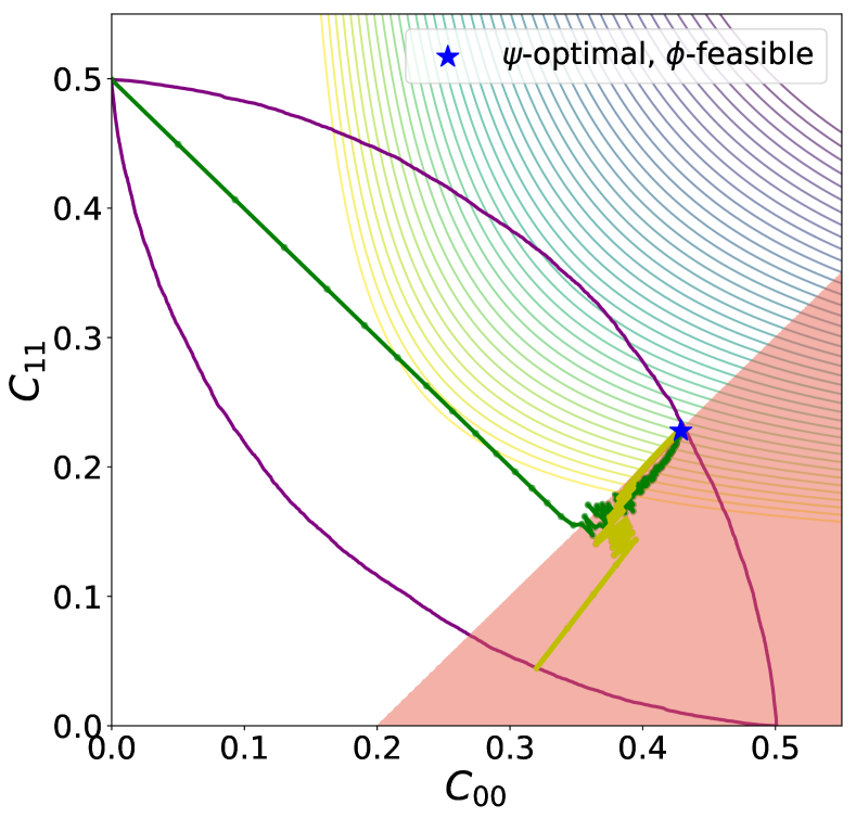
(a) SplitFW

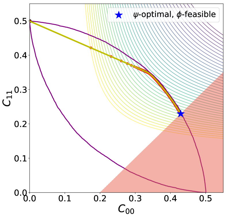
(b) ConGDA

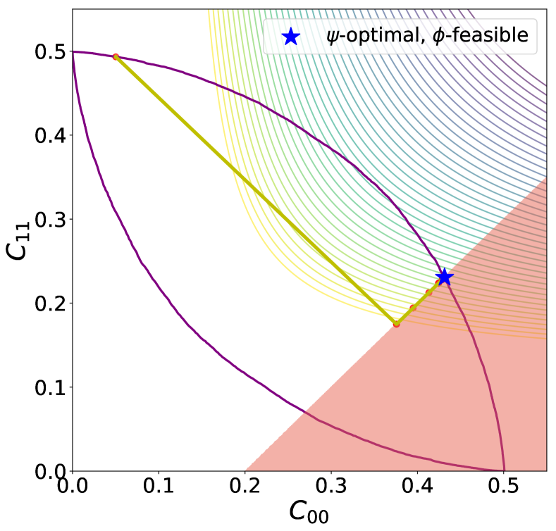
(c) ConEllipsoid

Figure 6: Illustration of the Split Frank-Wolfe (Algorithm 1), Constrained GDA (Algorithm 6) and Constrained Ellipsoid (Algorithm 7) algorithms in minimizing the H-mean loss $\psi^{\textup{{HM}}}$ subject to the constraint $C_{00}-C_{11}\geq 0.2$ on the NormBal distribution in Figure 2(b). The figures contain the space of achievable confusion matrices ${\mathcal{C}}$ (with purple colored boundary), along with the contours of $\psi^{\textup{{HM}}}$. The trajectory of the averaged confusion matrix ${\mathbf{C}}[\bar{h}^{t}]$ for the averaged classifier is shown in green, where $\bar{h}^{t}=h^{t}$ for Frank-Wolfe, $\bar{h}^{t}=\frac{1}{t}\sum_{\tau=1}^{t}h^{t}$ for GDA, and $\bar{h}^{t}=\frac{1}{t}\sum_{\tau=1}^{t}\alpha^{*}_{\tau}h^{\tau}$ for ellipsoid, with the optimal coefficients ${\boldsymbol{\alpha}}^{*}\in\operatorname{argmin}_{{\boldsymbol{\alpha}}\in\Delta_{t}:\,{\boldsymbol{\phi}}(\sum_{\tau=1}^{t}\alpha_{\tau}{\mathbf{C}}^{\tau})\leq{\mathbf{0}}}\psi\left(\sum_{\tau=1}^{t}\alpha_{\tau}{\mathbf{C}}^{\tau}\right)$ computed for iterates $1,\ldots t$. For SplitFW, we additionally plot the set of feasible confusion matrices ${\mathcal{F}}$ that satisfy the constraint (shaded red region), along with the trajectory of the the averaged auxiliary variables ${\mathbf{F}}^{t}$ (gold). The algorithms can be seen to converge to an optimal feasible solution.

5 Algorithms for Constrained Problems

We next present iterative algorithms for solving the constrained learning problem in OP2, which as noted earlier, can be viewed as a minimization problem over ${\mathcal{C}}$:

$$\min_{{\mathbf{C}}\in{\mathcal{C}},{\boldsymbol{\phi}}({\mathbf{C}})\leq{\mathbf{0}}}\psi({\mathbf{C}}).$$ (OP2*)

As in the previous section, we will assume access to an LMO with the properties in Definition 11.

A simple approach to solving OP2 for convex $\psi$’s and $\phi$’s is to formulate an equivalent convex-concave saddle point problem in terms of its Lagrangian:

$$\min_{{\mathbf{C}}\in{\mathcal{C}}}\max_{\boldsymbol{\lambda}\in{\mathbb{R}}_{+}^{K}}\,\psi({\mathbf{C}})+\sum_{k=1}^{K}\lambda_{k}\phi_{k}({\mathbf{C}})~{}=~{}\max_{\boldsymbol{\lambda}\in{\mathbb{R}}_{+}^{K}}\underbrace{\min_{{\mathbf{C}}\in{\mathcal{C}}}\,\psi({\mathbf{C}})+\sum_{k=1}^{K}\lambda_{k}\phi_{k}({\mathbf{C}})}_{\nu(\lambda)},$$

where $\lambda_{k}$ is the Lagrange multiplier for constraint $\phi_{k}$, and we use strong duality to exchange the ‘min’ and ‘max’. For a fixed $\boldsymbol{\lambda}$, the minimization over ${\mathbf{C}}$ is an unconstrained convex problem in ${\mathbf{C}}$. This resembles OP1 and can be solved with any of Algorithm 1–3 proposed in the previous section. One can therefore apply a standard gradient ascent procedure to maximize the dual function $\nu(\boldsymbol{\lambda})$, where the gradients w.r.t. $\boldsymbol{\lambda}$ can be computed by solving the minimization of ${\mathbf{C}}$. However, this vanilla dual-ascent approach does not enjoy strong convergence guarantees because of the multiple levels of nesting. For example, with the Frank-Wolfe based algorithm (Algorithm 1) for the inner minimization, this procedure would take ${\mathcal{O}}(1/\epsilon^{3})$ calls to the LMO to reach an ${\mathcal{O}}(\epsilon)$-optimal, ${\mathcal{O}}(\epsilon)$-feasible solution (Narasimhan, 2018).

In what follows, we describe four algorithms for solving OP2 which require fewer calls to the LMO than the vanilla approach described above (see Table 3 for a summary of our results). The proofs build on standard techniques for showing convergence of the respective optimization solvers, but need to additionally take into account the errors in the LMO calls and need to translate the dual-optimal solution guarantees to optimality and feasibility guarantees for the primal solution.

The proposed algorithms can be seen as “constrained” counterparts to the four unconstrained algorithms described in the previous section. All our algorithms will assume that the constraints $\phi_{k}({\mathbf{C}})$ are convex in ${\mathbf{C}}$. As a running example to illustrate our algorithms, we will use the task of maximizing the H-mean loss on the NormBal distribution described in Figure 2(b), subject to the constraint that coverage on class 1 be no more than 0.3. This constraint is linear in ${\mathbf{C}}$ and can be written as $C_{01}+C_{11}\leq 0.3$, or equivalently re-written as $C_{00}-C_{11}\geq 0.2$.

Table 3: Algorithms for the constrained problem in OP2, with the number calls to the LMO, and the optimality gap $\psi({\mathbf{C}}[\bar{h}])-\min_{{\mathbf{C}}\in{\mathcal{C}}}\psi({\mathbf{C}})$ and feasibility gap $\max_{k}\phi_{k}({\mathbf{C}}[\bar{h}])$ for the returned classifier $\bar{h}$. In rows 1–3, we assume $\psi$ is Lipschitz w.r.t. the $\ell_{2}$-norm, and in all rows, we assume that $\phi_{1},\ldots,\phi_{K}$ are convex and Lipschitz, and satisfy the strict feasibilty condition in Assumption 1. In row 4, $\psi({\mathbf{C}})\,=\,\frac{\langle{\mathbf{A}},{\mathbf{C}}\rangle}{\langle{\mathbf{B}},{\mathbf{C}}\rangle}$ with $\min_{{\mathbf{C}}\in{\mathcal{C}}}\langle{\mathbf{B}},{\mathbf{C}}\rangle>0$. We denote $\bar{d}=d+K$, and $\rho^{\textup{{eff}}}=\rho+\sqrt{d}\rho^{\prime}$.

Algorithm	Assumption on $\psi$	# LMO Calls	Opt. Gap	Feasibility Gap
Split Frank-Wolfe	Convex, Smooth	$\displaystyle{\mathcal{O}}\left(1/\epsilon^{2}\right)$	${\mathcal{O}}\left(\epsilon+\sqrt{\rho^{\textup{{eff}}}}\right)$	${\mathcal{O}}\left(\epsilon+\sqrt{\rho^{\textup{{eff}}}}\right)$
Con. GDA	Convex	$\displaystyle{\mathcal{O}}\left(K/\epsilon^{2}\right)$	${\mathcal{O}}\left(\epsilon+\rho^{\textup{{eff}}}\right)$	${\mathcal{O}}\left(\epsilon+\rho^{\textup{{eff}}}\right)$
Con. Ellipsoid	Convex	$\displaystyle{\mathcal{O}}\left(\bar{d}^{2}\log(\bar{d}/\epsilon)\right)$	${\mathcal{O}}\left(\epsilon+\rho^{\textup{{eff}}}\right)$	${\mathcal{O}}\left(\rho^{\textup{{eff}}})\right)$
Con. Bisection	Ratio-of-linear	$\displaystyle{\mathcal{O}}\left(K\log(1/\epsilon)/\epsilon^{2}\right)$	${\mathcal{O}}\left(\epsilon+\rho^{\textup{{eff}}}\right)$	${\mathcal{O}}\left(\epsilon+\rho^{\textup{{eff}}}\right)$

5.1 (Split) Frank-Wolfe Algorithm for Smooth Convex Metrics

In this section, we adapt the Frank-Wolfe approach in Algorithm 1 to constrained learning problems OP2 for smooth convex metrics $\psi$. The key idea is to pose OP2* as an optimization problem over the intersection of two sets:

$$\min_{{\mathbf{C}}\in{\mathcal{C}}:\,{\boldsymbol{\phi}}({\mathbf{C}})\leq{\mathbf{0}}}\psi({\mathbf{C}}) =\min_{{\mathbf{C}}\in{\mathcal{C}}\cap{\mathcal{F}}}\psi({\mathbf{C}}),$$ (4)

where ${\mathcal{F}}=\{{\mathbf{F}}\in\Delta_{d}\,|\,{\boldsymbol{\phi}}({\mathbf{F}})\leq{\mathbf{0}}\}$ is the set of all points in $\Delta_{d}$ that satisfy the $K$ inequality constraints. While the set ${\mathcal{F}}$ is convex (and so is the intersection ${\mathcal{C}}\cap{\mathcal{F}}$), we will not be able to apply the classical Frank-Wolfe method to this problem as we cannot directly solve a linear minimization over the intersection ${\mathcal{C}}\cap{\mathcal{F}}$. However, we already have access to an LMO for the set ${\mathcal{C}}$ alone, and performing a linear minimization over the set ${\mathcal{F}}$ amounts to solving a straight-forward convex program. We therefore adopt the Frank-Wolfe based variant proposed by Gidel et al. (2018) for optimizing a (smooth) convex function over the intersection of two convex sets with access to linear minimization oracles for the individual sets.

To this end, we introduce auxiliary variables ${\mathbf{F}}\in\Delta_{d}$ in (4) and decouple the two constraint sets, giving us the following equivalent optimization problem:

$$\min_{{\mathbf{C}}\in{\mathcal{C}},{\mathbf{F}}\in{\mathcal{F}}}\psi({\mathbf{C}})+\psi({\mathbf{F}})\enskip\text{s.t.}\enskip{\mathbf{C}}-{\mathbf{F}}=0.$$ (5)

We then define the augmented Lagrangian of the above problem as:

$$\mathcal{L}^{\textup{{aug}}}({\mathbf{C}},{\mathbf{F}},\boldsymbol{\lambda})=\psi({\mathbf{C}})+\psi({\mathbf{F}})+\langle\boldsymbol{\lambda},{\mathbf{C}}-{\mathbf{F}}\rangle+\dfrac{\zeta}{2}||{\mathbf{C}}-{\mathbf{F}}||_{2}^{2},$$ (6)

where $\boldsymbol{\lambda}$ is a vector of Lagrange multipliers for the equality constraints and $\zeta>0$ is a constant weight on the quadratic penalty term. We apply the approach of Gidel et al. (2018) to solve (5) by using a gradient ascent step to maximize $\mathcal{L}^{\textup{{aug}}}$ over $\boldsymbol{\lambda}$, a linear minimization step for ${\mathbf{C}}$ over ${\mathcal{C}}$, and a linear minimization step for ${\mathbf{F}}$ over ${\mathcal{F}}$.

Algorithm 5 Split Frank-Wolfe (SplitFW) Algorithm for OP2 with Smooth Convex $\psi$

1:  Input: $\psi,\phi_{1},\ldots,\phi_{k}:[0,1]^{d}\to[0,1]$, an LMO $\Omega$, $S=\{(x_{1},y_{1}),\ldots,(x_{N},y_{N})\}$, $T\in{\mathbb{N}}$, $\zeta,\eta>0$.

2:  Initialize: $(h^{0},{\mathbf{C}}^{0})=\Omega({\mathbf{L}}^{0};S)$ for an arbitrary loss matrix ${\mathbf{L}}^{0}$

3:  For $t=1$ to $T$ do

4:       ${\mathbf{L}}^{t}\,=\,\frac{\mathbf{a}^{t}}{\|\mathbf{a}\|_{2}},$ where $\mathbf{a}^{t}=\nabla_{\mathbf{C}}\mathcal{L}^{\textup{{aug}}}({\mathbf{C}}^{t-1},{\mathbf{F}}^{t-1},\boldsymbol{\lambda}^{t-1})$

5:       $(\widetilde{h}^{t},\widetilde{{\mathbf{C}}}^{t})\,=\,\Omega({\mathbf{L}}^{t};S)$

6:       $\widetilde{\mathbf{F}}^{t}=\operatorname{argmin}_{{\mathbf{F}}\in{\mathcal{F}}}\left\langle\mathbf{b}^{t},{\mathbf{F}}\right\rangle$, where $\mathbf{b}^{t}=\nabla_{\mathbf{F}}\mathcal{L}^{\textup{{aug}}}({\mathbf{C}}^{t-1},{\mathbf{F}}^{t-1},\boldsymbol{\lambda}^{t-1})$

7:       $\gamma^{t}=\operatorname{argmin}_{\gamma\in[0,1]}\mathcal{L}^{\textup{{aug}}}\big{(}(1-\gamma){\mathbf{C}}^{t-1}+\gamma\widetilde{\mathbf{C}}^{t},\ (1-\gamma){\mathbf{F}}^{t-1}+\gamma\widetilde{\mathbf{F}}^{t},\ \boldsymbol{\lambda}^{t-1}\big{)}$

8:       ${h}^{t}=\big{(}1-\gamma^{t}\big{)}{h}^{t-1}+\gamma^{t}\widetilde{h}^{t}$

9:       ${\mathbf{C}}^{t}=(1-\gamma^{t}){\mathbf{C}}^{t-1}+\gamma^{t}\widetilde{{\mathbf{C}}}^{t}$

10:       ${\mathbf{F}}^{t}=(1-\gamma^{t}){\mathbf{F}}^{t-1}+\gamma^{t}\widetilde{{\mathbf{F}}}^{t}$

11:       $\boldsymbol{\lambda}^{t}=\boldsymbol{\lambda}^{t-1}+\frac{\eta}{t}({\mathbf{C}}^{t}-{\mathbf{F}}^{t})$

12:  End For

13:  Output: $\bar{h}=h^{t_{*}}$ and $\bar{{\mathbf{C}}}={\mathbf{C}}^{t_{*}}$, where $t_{*}=\operatorname{argmin}_{t>T/2}||{\mathbf{C}}^{t}-{\mathbf{F}}^{t}||_{2}^{2}$

This procedure, outlined in Algorithm 5, is guaranteed to converge to an optimal feasible classifier under the assumption that there exists a confusion matrix which is strictly feasible.

Assumption 1 (Strict feasibility).

For some $r>0$, there exists a confusion matrix ${\mathbf{C}}^{\prime}\in{\mathcal{C}}$ such that $\max_{k\in[K]}\phi_{k}({\mathbf{C}}^{\prime})\leq-r$.

Theorem 16 (Convergence of SplitFW algorithm).

Fix $\epsilon>0$. Let $\psi:[0,1]^{d}{\rightarrow}[0,1]$ be convex, $\beta$-smooth and $L$-Lipschitz w.r.t. the $\ell_{2}$-norm, and let $\phi_{1},\ldots,\phi_{K}:[0,1]^{d}{\rightarrow}[-1,1]$ be convex and $L$-Lipschitz w.r.t. the $\ell_{2}$-norm. Let $\Omega$ in Algorithm 5 be a $(\rho,\rho^{\prime},\delta)$-approximate LMO for sample size $N$. Let $\bar{h}$ be a classifier returned by Algorithm 5 when run for $T$ iterations with some $\zeta>0$. Let the strict feasibility condition in Assumption 1 hold for radius $r>0$. Then, with probability $\geq 1-\delta$ over draw of $S\sim D^{N}$, after $T={\mathcal{O}}(1/\epsilon^{2})$ iterations:

$$\textbf{Optimality:}~{}~{}\psi({\mathbf{C}}[\bar{h}])\,\leq\,\min_{{\mathbf{C}}\in{\mathcal{C}},\phi_{k}({\mathbf{C}})\leq 0,\forall k}\,\psi({\mathbf{C}})\,+\,{\mathcal{O}}\left(\epsilon+\sqrt{\rho^{\textup{{eff}}}}\right);\vspace{-5pt}$$

$$\textbf{Feasibility:}~{}~{}\phi_{k}({\mathbf{C}}[\bar{h}])\,\leq\,{\mathcal{O}}\left(\epsilon+\sqrt{\rho^{\textup{{eff}}}}\right),~{}\forall k\in[K].$$

where $\rho^{\textup{{eff}}}=\rho+\sqrt{d}\rho^{\prime}$ and the ${\mathcal{O}}$ notation hides constant factors independent of $\rho,\rho^{\prime},T,d$ and $K$ for small enough $\rho,\rho^{\prime}$ and large $T$.

Proof.

See Appendix A.8 ∎

Unlike the Frank-Wolfe based algorithm for the unconstrained problem (see Theorem 12) which needed only ${\mathcal{O}}(1/\epsilon)$ calls to the LMO to reach an ${\mathcal{O}}(\epsilon+c)$-optimal solution, the proposed algorithm for handling constraints requires ${\mathcal{O}}(1/\epsilon^{2})$ calls to reach an ${\mathcal{O}}(\epsilon+c)$-optimal, feasible solution.

Figure 6(a) illustrates the trajectories of the algorithm applied to the previously described running example. As seen, both the iterates ${\mathbf{C}}^{t}$ and ${\mathbf{F}}^{t}$, representing the achievable and feasible confusion matrices respectively, are seen to converge to a solution that is optimal and feasible for the problem.

5.2 Gradient Descent-Ascent Algorithm for Non-smooth Convex Metrics

Next, we modify the gradient descent-ascent approach in Algorithm 2 to handle constraints. Our proposal is a slight variant of the oracle-based algorithm in Narasimhan et al. (2019) for optimizing with constraints. As before, we introduce slack variables ${\boldsymbol{\xi}}\in\Delta_{d}$ to decouple the functions $\psi,\phi_{1},\ldots,\phi_{K}$ from the confusion matrix ${\mathbf{C}}$, and re-write OP2* as:

$$\min_{{\mathbf{C}}\in{\mathcal{C}}:\,{\boldsymbol{\phi}}({\mathbf{C}})\leq{\mathbf{0}}}\psi({\mathbf{C}}) =\min_{\begin{subarray}{c}{\mathbf{C}}\in{\mathcal{C}},\,{\boldsymbol{\xi}}\in\Delta_{d}\\ {\boldsymbol{\xi}}={\mathbf{C}},\,\phi_{k}({\boldsymbol{\xi}})\leq 0,\forall k\end{subarray}.}\psi({\boldsymbol{\xi}})$$ (7)

We then define the Lagrangian for the above problem with multipliers $\boldsymbol{\lambda}\in{\mathbb{R}}^{d}$ for the $d$ equality constraints and ${\boldsymbol{\mu}}\in{\mathbb{R}}_{+}^{K}$ for the $K$ inequality constraints:

$$\mathcal{L}^{\textup{{con}}}({\mathbf{C}},{\boldsymbol{\xi}},\boldsymbol{\lambda},{\boldsymbol{\mu}}) =\psi({\boldsymbol{\xi}})+\langle\boldsymbol{\lambda},{\mathbf{C}}-{\boldsymbol{\xi}}\rangle+\langle{\boldsymbol{\mu}},\boldsymbol{\phi}({\boldsymbol{\xi}})\rangle,$$ (8)

and re-formulate (7) as the following min-max problem:

$$\min_{{\mathbf{C}}\in{\mathcal{C}},\phi_{k}({\mathbf{C}})\leq 0,\forall k} =\min_{{\mathbf{C}}\in{\mathcal{C}},\,{\boldsymbol{\xi}}\in\Delta_{d}}\,\max_{\boldsymbol{\lambda}\in{\mathbb{R}}^{d},{\boldsymbol{\mu}}\in{\mathbb{R}}_{+}^{K}}\,\mathcal{L}^{\textup{{con}}}({\mathbf{C}},{\boldsymbol{\xi}},\boldsymbol{\lambda},{\boldsymbol{\mu}}).$$ (9)

The gradient descent-ascent procedure for solving an approximate saddle point of (9) is shown in Algorithm 2 and enjoys the following convergence guarantee for a convex, non-smooth metric $\psi$:

Theorem 17 (Convergence of ConGDA algorithm).

Fix $\epsilon\in(0,1)$. Let $\psi:[0,1]^{d}{\rightarrow}[-1,1]$ and $\phi_{1},\ldots,\phi_{K}:[0,1]^{d}{\rightarrow}[-1,1]$ be convex and $L$-Lipschitz w.r.t. the $\ell_{2}$-norm. Let $\Omega$ in Algorithm 6 be a $(\rho,\rho^{\prime},\delta)$-approximate LMO for sample size $N$. Suppose the strict feasibility condition in Assumption 1 holds for radius $r>0$. Let the space of Lagrange multipliers $\Lambda=\{\boldsymbol{\lambda}\in{\mathbb{R}}^{d}\,|\,\|\boldsymbol{\lambda}\|_{2}\leq 2L(1+1/r)\}$, and $\Xi=\{{\boldsymbol{\mu}}\in{\mathbb{R}}_{+}^{K}\,|\,\|{\boldsymbol{\mu}}\|_{1}\leq 2/r\}$. Let $\bar{h}$ be a classifier returned by Algorithm 6 when run for $T$ iterations, with step-sizes $\eta=\frac{1}{\bar{L}\sqrt{2T}}$ and $\eta^{\prime}=\frac{\bar{L}}{(1+2\sqrt{K})\sqrt{2T}}$, where $\bar{L}=4(1+1/r)L+2/r$. Then with probability $\geq 1-\delta$ over draw of $S\sim D^{N}$, after $T={\mathcal{O}}(K/\epsilon^{2})$ iterations:

$$\textbf{Optimality:}~{}~{}\psi({\mathbf{C}}[\bar{h}])\,\leq\,\min_{{\mathbf{C}}\in{\mathcal{C}}:\,{\boldsymbol{\phi}}({\mathbf{C}})\leq{\mathbf{0}}}\,\psi({\mathbf{C}})\,+\,{\mathcal{O}}\left(\epsilon+\rho^{\textup{{eff}}}\right);$$

$$\textbf{Feasibility:}~{}~{}\phi_{k}({\mathbf{C}}[\bar{h}])\,\leq\,{\mathcal{O}}\left(\epsilon+\rho^{\textup{{eff}}}\right),\forall k\in[K].$$

where $\rho^{\textup{{eff}}}=\rho+\sqrt{d}\rho^{\prime}$ and the ${\mathcal{O}}$ notation hides constant factors independent of $\rho,\rho^{\prime},T,d$ and $K$.

Proof.

See Appendix A.9. ∎

Algorithm 6 Constrained GDA (ConGDA) Algorithm for OP2 with Non-smooth Convex $\psi$

1:  Input: $\psi,\phi_{1},\ldots,\phi_{K}:[0,1]^{d}\to[0,1]$, an LMO $\Omega$, $S=\{(x_{1},y_{1}),\ldots,(x_{N},y_{N})\}$, $T$, space of Lagrange multipliers $\Lambda\subset{\mathbb{R}}^{d},\Xi\subset{\mathbb{R}}_{+}^{K}$

2:  Parameters: Step-sizes $\eta_{{\boldsymbol{\xi}}},\eta_{\boldsymbol{\lambda}},\eta_{{\boldsymbol{\mu}}}>0$

3:  Initialize: $(h^{0},{\mathbf{C}}^{0})=\Omega({\mathbf{L}}^{0};S)$ for an arbitrary loss matrix ${\mathbf{L}}^{0}$

4:  For $t=1$ to $T$ do

5:       ${\mathbf{L}}^{t}\,=\,\frac{\boldsymbol{\lambda}^{t-1}}{\|\boldsymbol{\lambda}^{t-1}\|_{2}}$

6:       $(h^{t},{\mathbf{C}}^{t})\,=\,\Omega({\mathbf{L}}^{t};S)$

7:       $\widetilde{{\boldsymbol{\xi}}}\,=\,{\boldsymbol{\xi}}^{t-1}\,-\,\eta_{\boldsymbol{\xi}}\nabla_{{\boldsymbol{\xi}}}\mathcal{L}^{\textup{{con}}}({\mathbf{C}}^{t},{\boldsymbol{\xi}}^{t-1},\boldsymbol{\lambda}^{t-1},{\boldsymbol{\mu}}^{t-1})$;      ${\boldsymbol{\xi}}^{t+1}\,\in\,\operatorname{argmin}_{{\boldsymbol{\xi}}\in[0,1]^{d}}\,\|{\boldsymbol{\xi}}-\widetilde{{\boldsymbol{\xi}}}\|_{2}$

8:       $\widetilde{\boldsymbol{\lambda}}\,=\,\boldsymbol{\lambda}^{t-1}\,+\,\eta_{\boldsymbol{\lambda}}\nabla_{\boldsymbol{\lambda}}\mathcal{L}^{\textup{{con}}}({\mathbf{C}}^{t},{\boldsymbol{\xi}}^{t-1},\boldsymbol{\lambda}^{t-1},{\boldsymbol{\mu}}^{t-1})$;      $\boldsymbol{\lambda}^{t+1}\,\in\,\operatorname{argmin}_{\boldsymbol{\lambda}\in\Lambda}\|\boldsymbol{\lambda}-\widetilde{\boldsymbol{\lambda}}\|_{2}$

9:       $\widetilde{{\boldsymbol{\mu}}}^{t}\,=\,{\boldsymbol{\mu}}^{t-1}\,+\,\eta_{\boldsymbol{\mu}}\nabla_{{\boldsymbol{\mu}}}\mathcal{L}^{\textup{{con}}}({\mathbf{C}}^{t},{\boldsymbol{\xi}}^{t-1},\boldsymbol{\lambda}^{t-1},{\boldsymbol{\mu}}^{t-1})$;      ${\boldsymbol{\mu}}^{t+1}\,\in\,\operatorname{argmin}_{{\boldsymbol{\mu}}\in\Xi}\|{\boldsymbol{\mu}}-\widetilde{{\boldsymbol{\mu}}}\|_{2}$

10:  End For

11:  Output: $\bar{h}=\frac{1}{T}\sum_{t=1}^{T}h^{t}$

Figure 6(b) shows the trajectory of the iterates of the algorithm on the same running example used for the SplitFW algorithm. The algorithm is seen to converge to an optimal-feasible classifier.

5.3 Ellipsoid Algorithm for Non-smooth Convex Metrics

Our next algorithm extends the ellipsoid method in Algorithm 3 to handle constraints ${\boldsymbol{\phi}}({\mathbf{C}})\leq{\mathbf{0}}$. We use the Lagrangian $\mathcal{L}^{\textup{{con}}}({\mathbf{C}},{\boldsymbol{\xi}},\boldsymbol{\lambda},{\boldsymbol{\mu}})$ for the constrained problem defined in the previous section in (8), and work with its dual function $f$:

$$f^{\textup{{con}}}(\boldsymbol{\lambda},{\boldsymbol{\mu}}) =\begin{cases}\min_{{\mathbf{C}}\in{\mathcal{C}},\,{\boldsymbol{\xi}}\in\Delta_{d}}\mathcal{L}^{\textup{{con}}}({\mathbf{C}},{\boldsymbol{\xi}},\boldsymbol{\lambda},{\boldsymbol{\mu}})&\text{ if }{\boldsymbol{\mu}}\geq 0\\ -\infty&\text{ otherwise}\end{cases},$$

where we note that the Lagrange multipliers ${\boldsymbol{\mu}}$ for the $K$ inequality constraints are not allowed to be negative.

Following the unconstrained case, we seek to maximize the dual function over $\boldsymbol{\lambda}\in{\mathbb{R}}^{d}$ and over ${\boldsymbol{\mu}}\in{\mathbb{R}}_{+}^{K}$. Because $f^{\textup{{con}}}$ is concave in $\boldsymbol{\lambda}$ and ${\boldsymbol{\mu}}$, we can employ the ellipsoid method with the JLE subroutine in Algorithm 3(a) to maximize $f^{\textup{{con}}}(\boldsymbol{\lambda},{\boldsymbol{\mu}})$, and use a post-processing step to convert the dual solution to a near-optimal and near-feasible solution for the primal problem. As shown in Algorithm 7, at each iteration, the procedure maintains an ellipsoid containing the maximizer of $f^{\textup{{con}}}$, with the current iterate $[\boldsymbol{\lambda}^{t},{\boldsymbol{\mu}}^{t}]$ serving as the center of the ellipsoid

Lines 5 to 10 of the algorithm simply ensure the iterate $[\boldsymbol{\lambda}^{t},{\boldsymbol{\mu}}^{t}]$ stays within the initial ellipsoid, and ${\boldsymbol{\mu}}^{t}$ remains non-negative. As before, to compute a super-gradient for $f$ at a given $[\boldsymbol{\lambda}^{t},{\boldsymbol{\mu}}^{t}]$, we compute ${\mathbf{C}}^{t}\in\operatorname{argmin}_{{\mathbf{C}}\in{\mathcal{C}}}\langle\boldsymbol{\lambda}^{t},{\mathbf{C}}\rangle$ and ${\boldsymbol{\xi}}^{t}\in\operatorname{argmin}_{{\boldsymbol{\xi}}\in\Delta_{d}}\psi({\boldsymbol{\xi}})-\langle\boldsymbol{\lambda}^{t},{\boldsymbol{\xi}}\rangle+\langle{\boldsymbol{\mu}}^{t},{\boldsymbol{\phi}}({\boldsymbol{\xi}})\rangle$, and evaluate $[{\mathbf{C}}^{t}-{\boldsymbol{\xi}}^{t},{\boldsymbol{\phi}}({\boldsymbol{\xi}}^{t})]$. Note that ${\mathbf{C}}^{t}$ can be obtained via a linear minimization oracle over ${\mathcal{C}}$ and ${\boldsymbol{\xi}}^{t}$ is the solution of a convex program that has no dependence on the data distribution. The approximate nature of the LMO (and in turn the supergradient of $f^{\textup{{con}}}$) require a modified proof from the standard ellipsoid to argue that the errors at each iteration do not add up catastrophically. The dual solution is converted to a primal-feasible solution in line 16 of the algorithm by solving a convex optimization problem that requires no access to the training data.

Figure 7 illustrates the working of the algorithm. Note that the initial classifier $h^{0}$ can be any classifier, as it is the result of the LMO where the loss is the zero matrix. We assume here that the initial classifier $h^{0}$ is strictly feasible for convenience.

Algorithm 7 Constrained Ellipsoid (ConEllipsoid) Algorithm for OP2 with Non-smooth Convex $\psi$

1:  Input: $\psi:[0,1]^{d}\to[0,1]$, an LMO $\Omega$, $S=\{(x_{1},y_{1}),\ldots,(x_{N},y_{N})\},T$

2:  Parameters: Initial ellipsoid radius $a$, a strictly feasible classifier $h^{0}$

3:  Initialize: ${\boldsymbol{\lambda}}^{0}={\mathbf{0}}_{d},{{\boldsymbol{\mu}}}^{0}=0$, ${{\mathbf{A}}}^{0}=a^{2}{\mathbf{I}}_{d+K}$, ${\mathbf{C}}^{0}={{\mathbf{C}}}[h^{0}]$

4:  For $t=0$ to $T-1$:

5:       If $\|[{\boldsymbol{\lambda}}^{t},{{\boldsymbol{\mu}}}^{t}]\|_{2}>a$:

6:           ${{\mathbf{A}}}^{t+1},[{\boldsymbol{\lambda}}^{t+1},{{\boldsymbol{\mu}}}^{t+1}]=\text{JLE}({{\mathbf{A}}}^{t},[{\boldsymbol{\lambda}}^{t},{{\boldsymbol{\mu}}}^{t}],[-{\boldsymbol{\lambda}}^{t},-{{\boldsymbol{\mu}}}^{t}])$

7:           $h^{t},{\mathbf{C}}^{t}=h^{0},{\mathbf{C}}^{0}$ ; continue

8:       Else If ${{\boldsymbol{\mu}}}^{t}\ngeq{\mathbf{0}}$ :

9:           ${{\mathbf{A}}}^{t+1},[{\boldsymbol{\lambda}}^{t+1},{{\boldsymbol{\mu}}}^{t+1}]=\text{JLE}({{\mathbf{A}}}^{t},[{\boldsymbol{\lambda}}^{t},{{\boldsymbol{\mu}}}^{t}],[{\mathbf{0}}_{d},\text{pos}(-{\boldsymbol{\mu}}^{t})])$, where $\text{pos}(u)=\max(u,0)$.

10:           $h^{t},{\mathbf{C}}^{t}=h^{0},{\mathbf{C}}^{0}$ ; continue

11:      Else:

12:           $(h^{t},{\mathbf{C}}^{t})=\Omega(\boldsymbol{\lambda}^{t},S)$

13:           ${\boldsymbol{\xi}}^{t}=\operatorname{argmin}_{{\boldsymbol{\xi}}\in\Delta_{d}}\psi({\boldsymbol{\xi}})-\langle\boldsymbol{\lambda}^{t},{\boldsymbol{\xi}}\rangle+\langle{\boldsymbol{\mu}}^{t},\boldsymbol{\phi}({\boldsymbol{\xi}})\rangle$

14:           ${{\mathbf{A}}}^{t+1},[{\boldsymbol{\lambda}}^{t+1},{{\boldsymbol{\mu}}}^{t+1}]=\text{JLE}({\mathbf{A}}^{t},[\boldsymbol{\lambda}^{t},{\boldsymbol{\mu}}^{t}],[{\mathbf{C}}^{t}-{\boldsymbol{\xi}}^{t},\boldsymbol{\phi}({\boldsymbol{\xi}}^{t})])$

15:  End For

16:  ${\boldsymbol{\alpha}}^{*}\in\underset{{\boldsymbol{\alpha}}\in\Delta_{T}:\,{\boldsymbol{\phi}}(\sum_{t}\alpha_{t}{\mathbf{C}}^{t})\leq{\mathbf{0}}}{\operatorname{argmin}}\psi\left(\sum_{t=0}^{T-1}\alpha_{t}{\mathbf{C}}^{t}\right)$

17:  Ouput: $\bar{h}=\sum_{t=0}^{T-1}\alpha^{*}_{t}h^{t}$

Theorem 18 (Convergence of ConEllipsoid).

Fix $\epsilon\in(0,1)$. Let $\psi:[0,1]^{d}{\rightarrow}[0,1],\phi_{1},\ldots,\phi_{K}:[0,1]^{d}{\rightarrow}[-1,1]$ be convex and $L$-Lipschitz w.r.t. the $\ell_{2}$ norm. Let $\Omega$ in Algorithm 6 be a $(\rho,\rho^{\prime},\delta)$-approximate LMO for sample size $N$. Suppose the strict feasibility condition in Assumption 1 holds for some $r>0$. Let the initial classifier $h^{0}$ satisfy this condition, i.e. ${\boldsymbol{\phi}}({\mathbf{C}}[h^{0}])\leq-r$ and ${\mathbf{C}}[h^{0}]={\mathbf{C}}^{0}$. Let $\bar{d}=d+K$. Let $\bar{h}$ be the classifier returned by Algorithm 7 when run for $T>2\bar{d}^{2}\log(\frac{\bar{d}}{\epsilon})$ iterations with initial radius $a>2(L+\frac{L+1}{r})$. Then with probability $\geq 1-\delta$ over draw of $S\sim D^{N}$, we have

$$\textbf{Optimality:}~{}~{}\psi({\mathbf{C}}[\bar{h}])\, \leq\,\min_{{\mathbf{C}}\in{\mathcal{C}}:\,\phi_{k}({\mathbf{C}})\leq 0,\forall k}\,\psi({\mathbf{C}})+{\mathcal{O}}(\epsilon+\rho^{\textup{{eff}}});$$

$$\textbf{Feasibility:}~{}~{}\phi_{k}({\mathbf{C}}[\bar{h}])\, \leq\,{\mathcal{O}}(\rho^{\textup{{eff}}}),~{}\forall k\in[K],$$

where $\rho^{\textup{{eff}}}=\rho+\sqrt{d}\rho^{\prime}$ and the ${\mathcal{O}}$ notation hides constant factors independent of $\rho,\rho^{\prime},T,d$ and $K$.

Proof.

See Appendix A.10. ∎

The theorem above gives guarantees on the convergence of the constrained ellipsoid algorithm to the optimal feasible solution. Notice the exponential convergence rate in $1/\epsilon$ at the cost of a quadratic dependence on dimension $d$ and number of constraints $K$. Figure 6(c) shows the trajectory of the iterates of the algorithm on the same running example used previously. The algorithm is clearly seen to converge to an optimal-feasible classifier.

5.4 Bisection Algorithm for Fractional-linear Metrics

The final constrained algorithm we describe is a straightforward extension of the bisection method in Algorithm 4 for ratio-of-linear performance measures that can be written in the form $\psi({\mathbf{C}})=\frac{\langle{\mathbf{A}},{\mathbf{C}}\rangle}{\langle{\mathbf{B}},{\mathbf{C}}\rangle}$ for some ${\mathbf{A}},{\mathbf{B}}\in{\mathbb{R}}^{d}$. The key observation here is that testing whether the optimal solution to the constrained problem OP2* with a ratio-of-linear $\psi$ is greater than a threshold $\gamma$ is equivalent to minimizing a linear metric with constraints:

$$\min_{{\mathbf{C}}\in{\mathcal{C}}:\,{\boldsymbol{\phi}}({\mathbf{C}})\leq{\mathbf{0}}}\psi({\mathbf{C}})\geq\gamma\Longleftrightarrow\min_{{\mathbf{C}}\in{\mathcal{C}}:\,{\boldsymbol{\phi}}({\mathbf{C}})\leq{\mathbf{0}}}\langle{\mathbf{A}}-\gamma{\mathbf{B}},{\mathbf{C}}\rangle\geq 0.$$

The latter can be solved using any of constrained learning methods outlined Algorithms 5–7. Therefore one can employ the bisection method as before to conduct a binary search for the minimal value (and minimizer) of $\psi({\mathbf{C}})$ by calling one of these algorithms at each step. We outline this procedure in Algorithm 8, with the ConGDA method (Algorithm 6) used for the inner minimization.

We then have the following convergence guarantee:

Theorem 19 (Convergence of ConBisection algorithm).

Fix $\epsilon\in(0,1)$. Let $\psi:[0,1]^{d}{\rightarrow}[0,1]$ be such that $\psi({\mathbf{C}})\,=\,\frac{\langle{\mathbf{A}},{\mathbf{C}}\rangle}{\langle{\mathbf{B}},{\mathbf{C}}\rangle}$, where ${\mathbf{A}},{\mathbf{B}}\in[0,1]^{d}$, and $\min_{{\mathbf{C}}\in{\mathcal{C}}}{\langle{\mathbf{B}},{\mathbf{C}}\rangle}\,=\,b$ for some $b>0$. Let $\phi_{1},\ldots,\phi_{K}:[0,1]^{d}{\rightarrow}[-1,1]$ be convex and $L$-Lipschitz w.r.t. the $\ell_{2}$-norm. Let $\Omega$ in Algorithm 8 be a $(\rho,\rho^{\prime},\delta)$-approximate LMO for sample size $N$. Suppose the strict feasibility condition in Assumption 1 holds for some $r>0$. Let $\Lambda$, $\Xi$, $\eta$ and $\eta^{\prime}$ in the call to Algorithm 6 be set as in Theorem 17 with Lipschitz constant $L^{\prime}=\max\{L,\|{\mathbf{A}}\|_{2}+\|{\mathbf{B}}\|_{2}\}$. Let $\bar{h}$ be a classifier returned by Algorithm 8 when run for $T$ outer iterations and $T^{\prime}$ inner iterations. Then with probability $\geq 1-\delta$ over draw of $S\sim D^{N}$, after $T=\log(1/\epsilon)$ outer iterations and $T^{\prime}={\mathcal{O}}(K/\epsilon^{2})$ inner iterations:

$$\textbf{Optimality}:~{}~{}\psi({\mathbf{C}}[\bar{h}])\,\leq\,\min_{{\mathbf{C}}\in{\mathcal{C}}:\,{\boldsymbol{\phi}}({\mathbf{C}})\leq{\mathbf{0}}}\,\psi({\mathbf{C}})\,+\,{\mathcal{O}}\left(\epsilon+\rho^{\textup{{eff}}}\right);\vspace{-5pt}$$

$$\textbf{Feasibility}:~{}~{}\phi_{k}({\mathbf{C}}[\bar{h}])\,\leq\,{\mathcal{O}}\left(\epsilon+\rho^{\textup{{eff}}}\right),~{}\forall k\in[K],$$

where $\rho^{\textup{{eff}}}=\rho+\sqrt{d}\rho^{\prime}$ and the ${\mathcal{O}}$ notation hides constant factors independent of $\rho,\rho^{\prime},T,d$ and $K$.

Proof.

See Appendix A.11. ∎

Algorithm 8 Constrained Bisection (ConBisection) Algorithm for OP2 with Ratio-of-linear $\psi$

1:  Input: $\psi:[0,1]^{d}{\rightarrow}[0,1]$ s.t.  $\psi({\mathbf{C}})=\frac{\langle{\mathbf{A}},{\mathbf{C}}\rangle}{\langle{\mathbf{B}},{\mathbf{C}}\rangle}$ with ${\mathbf{A}},{\mathbf{B}}\in{\mathbb{R}}^{d}$ and $\phi_{1},\ldots,\phi_{K}:[0,1]^{d}{\rightarrow}[0,1]$

2:              an LMO $\Omega$, $S=\{(x_{1},y_{1}),\ldots,(x_{N},y_{N})\}$, $T$, $T^{\prime}$, ConGDA parameters: $\Lambda$, $\Xi$, $\eta$ and $\eta^{\prime}$

3:  Initialize: $\alpha^{0}=0,\beta^{0}=1,$ a classifier $h^{0}$ that satisfies the constraints, i.e. ${\boldsymbol{\phi}}({\mathbf{C}}[h^{0}])\leq{\mathbf{0}}$

4:  For $t=1~{}\text{to}~{}T$ do

5:       $\gamma^{t}=(\alpha^{t-1}+\beta^{t-1})/{2}$

6:       $({g}^{t},{\mathbf{C}}^{t})\,=\,\text{ConGDA}(\psi^{\prime},{\boldsymbol{\phi}},S,\Omega,T^{\prime},\Lambda,\Xi,\eta,\eta^{\prime}),$ where $\psi^{\prime}({\mathbf{C}})=\langle{\mathbf{A}}\,-\,\gamma^{t}{\mathbf{B}},{\mathbf{C}}\rangle$

7:       If $\psi({\mathbf{C}}^{t})\geq\gamma^{t}$  then  $\alpha^{t}=\gamma^{t},~{}~{}\beta^{t}=\beta^{t-1},~{}~{}h^{t}={g}^{t}$

8:                                else  $\alpha^{t}=\alpha^{t-1},~{}~{}\beta^{t}=\gamma^{t},~{}~{}h^{t}=h^{t-1}$

9:  End For

10:  Output: $\bar{h}=h^{T}$

6 Plug-in Based Linear Minimization Oracle

All the learning algorithms we have presented have assumed access to an approximate linear minimization oracle (LMO) (see Definition 11). In this section, we describe a practical plug-in based LMO with the desired approximation properties. This method seeks to approximate the Bayes-optimal classifier for the given linear metric using an estimate $\widehat{{\boldsymbol{\eta}}}:{\mathcal{X}}{\rightarrow}\Delta_{n}$ of the conditional-class probability distribution $\eta_{i}(X)={\mathbf{P}}(Y=i|X)$.

Specifically, for a flattened loss matrix ${\mathbf{L}}\in{\mathbb{R}}_{+}^{d}$, where $L_{n(i-1)+j}$ is the cost of predicting class $j$ when the true class is $i$, we have from Proposition 5 that the Bayes-optimal classifier is given by $h^{*}(x)=\operatorname{argmin}^{*}_{j\in[n]}\sum_{i=1}^{n}\eta_{i}(x)L_{n(i-1)+j}$. The plug-in based LMO outlined in Algorithm 9 approximates this classifier with the class probability model $\widehat{{\boldsymbol{\eta}}}$. The classifier and confusion matrix returned by the algorithm satisfy the LMO approximation properties laid out in Definition 11:

Theorem 20 (Regret bound for plug-in LMO).

Fix $\delta\in(0,1)$. Then with probability $\geq 1-\delta$ over draw of sample $S\sim D^{N}$, for any loss matrix ${\mathbf{L}}\in{\mathbb{R}}^{d}$, the classifier and confusion matrix $(\widehat{g},\widehat{\boldsymbol{\Gamma}})$ returned by Algorithm 9 satisfies:

$$\langle{\mathbf{L}},{\mathbf{C}}[\widehat{g}]\rangle\,\leq\,\min_{h:{\mathcal{X}}{\rightarrow}\Delta_{n}}\langle{\mathbf{L}},{\mathbf{C}}[h]\rangle+\|{\mathbf{L}}\|_{\infty}{\mathbf{E}}_{X}\big{[}\big{\|}\widehat{{\boldsymbol{\eta}}}(X)\,-\,{\boldsymbol{\eta}}(X)\big{\|}_{1}\big{]};\vspace{-5pt}$$

$$\|{\mathbf{C}}[\widehat{g}]\,-\,\widehat{{\boldsymbol{\Gamma}}}\|_{\infty}\,\leq\,{\mathcal{O}}\bigg{(}\sqrt{\displaystyle\frac{d\log(n)\log(N)+\log(d/\delta)}{N}}\bigg{)}.$$

Proof.

See Appendix A.12 ∎

Algorithm 9 Plug-in Based LMO

1:  Input: Loss matrix ${\mathbf{L}}\in{\mathbb{R}}_{+}^{d}$, Class prob. model $\widehat{{\boldsymbol{\eta}}}:{\mathcal{X}}{\rightarrow}\Delta_{n}$, $S=\{(x_{1},y_{1}),\ldots,(x_{N},y_{N})\}$

2:  Construct classifier $\widehat{g}(x)\,=\,\operatorname{argmin}^{*}_{j\in[n]}\sum_{i=1}^{n}\widehat{\eta}_{i}(x)L_{n(i-1)+j}$

3:  $\widehat{{\boldsymbol{\Gamma}}}=\textup{{vec}}\big{(}\widehat{{\mathbf{C}}}^{S}[\widehat{g}]\big{)}$

4:  Output: $\widehat{g}$, $\widehat{{\boldsymbol{\Gamma}}}$

6.1 Consistency of Proposed Algorithms with Plug-in LMO

Theorem 20 tells us that the quality of the classifier $\widehat{g}$ returned by the plug-in based LMO depends on the estimation error ${\mathbf{E}}_{X}\big{[}\big{\|}\widehat{{\boldsymbol{\eta}}}(X)\,-\,{\boldsymbol{\eta}}(X)\big{\|}_{1}\big{]}$, which measures the gap between the class probability model $\widehat{{\boldsymbol{\eta}}}$ and the true conditional class probabilities ${\boldsymbol{\eta}}$. By combining this result with Theorem 12–18, we can show that the algorithms described in Sections 4 and 5, when used with the plug-in based LMO, are statistically consistent. For the sake of brevity, we present the consistency analysis for the GDA algorithm and its constrained counter-part alone. The analysis for the other algorithms follow identical steps.

Let $S_{1}$ and $S_{2}$ be equal splits of the training sample $S$, and suppose we provide $S_{1}$ to the outer optimization methods in Algorithms 2 and 6 and $S_{2}$ to the inner LMO implemented using the plug-in method in Algorithm 9. We then have:

Corollary 21 (Regret bound for GDA algorithm).

Let $\psi:[0,1]^{d}{\rightarrow}[0,1]$ be convex and $L$-Lipschitz w.r.t. the $\ell_{2}$-norm. Let the LMO $\Omega$ in Algorithm 2 be a plug-in based LMO (as in Algorithm 9) with a CPE argument $\widehat{\boldsymbol{\eta}}$. Let $\bar{h}$ be a classifier returned by Algorithm 2 when run for $T$ iterations with the parameter settings in Theorem 13. Then with probability $\geq 1-\delta$ over draw of $S\sim D^{N}$, after $T={\mathcal{O}}(N)$ iterations:

$$\psi({\mathbf{C}}[\bar{h}])\,\leq\,\min_{{\mathbf{C}}\in{\mathcal{C}}}\,\psi({\mathbf{C}})\,+\,{{\mathcal{O}}}\left({\mathbf{E}}_{X}[\|\widehat{\boldsymbol{\eta}}(X)-{\boldsymbol{\eta}}(X)\|_{1}]+\sqrt{d}\sqrt{\frac{d\log(n)\log(N)+\log(d/\delta)}{N}}\right).$$

Corollary 22 (Regret bound for ConGDA algorithm).

Let $\psi:[0,1]^{d}{\rightarrow}[0,1]$ and $\phi_{1},\ldots,\phi_{K}:[0,1]^{d}{\rightarrow}[-1,1]$ be convex and $L$-Lipschitz. Let the LMO $\Omega$ in Algorithm 2 be a plug-in based LMO (as in Algorithm 9) with a CPE argument $\widehat{\boldsymbol{\eta}}$. Let $\bar{h}$ be a classifier returned by Algorithm 6 when run for $T$ iterations with the parameter settings in Theorem 17. Then with probability $\geq 1-\delta$ over draw of $S\sim D^{N}$, after $T={\mathcal{O}}(KN)$ iterations:

$$\psi({\mathbf{C}}[\bar{h}])\,\leq\,\min_{{\mathbf{C}}\in{\mathcal{C}}}\,\psi({\mathbf{C}})\,+\,{\mathcal{O}}\left({\mathbf{E}}_{X}[\|\widehat{\boldsymbol{\eta}}(X)-{\boldsymbol{\eta}}(X)\|_{1}]+\sqrt{d}\sqrt{\frac{d\log(n)\log(N)+\log(d/\delta)}{N}}\right);\vspace{-5pt}$$

$$\phi_{k}({\mathbf{C}}[\bar{h}])\,\leq\,{\mathcal{O}}\left({\mathbf{E}}_{X}[\|\widehat{\boldsymbol{\eta}}(X)-{\boldsymbol{\eta}}(X)\|_{1}]+\sqrt{d}\sqrt{\frac{d\log(n)\log(N)+\log(d/\delta)}{N}}\right),~{}\forall k\in[K].$$

When the class probability model $\widehat{{\boldsymbol{\eta}}}$ used by the LMO is learned by an algorithm that guarantees ${\mathbf{E}}_{X}[\|\widehat{{\boldsymbol{\eta}}}(X)-{\boldsymbol{\eta}}(X)\|_{1}]{\rightarrow}0$ as $N{\rightarrow}\infty$, then Algorithm 2 is statistically consistent for the unconstrained problem in (OP1), and Algorithm 6 is statistically consistent for the constrained problem in (OP2). The property that the learned class probability estimation error goes to zero in the large sample limit is true for any algorithm that minimizes a strictly proper composite multiclass loss (e.g. the standard cross-entropy loss) over a suitably large function class (Vernet et al., 2011).

While our consistency results require that the samples used by the outer optimization method and the inner LMO to be drawn independently, this may be inconvenient in real-world applications where data is scarce and limited. In practice, we find that using the same sample for both the outer and inner routines does not hurt performance, and this is the approach we adopt in our experiments.

A practical advantage of the plug-in based LMO is that one can pre-train the class probability model $\widehat{{\boldsymbol{\eta}}}$ and re-use the same model each time the LMO is invoked. In practice, there are other off-the-shelf algorithms that one can use to implement the LMO, such as cost-weighted decision trees (Ting, 2002) and those based on optimizing a cost-weighted surrogate loss (e.g. Lee et al. (2004)), which require training a new classifier for each given loss vector ${\mathbf{L}}$. While a majority of our experiments will use a plug-in based LMO, we also explore the use of cost-weighted surrogate losses for implementing the LMO.

7 Extension to Fairness Metrics and Other Refinements

To keep the exposition concise, we have so far focused on metrics defined by a function of the overall confusion matrix ${\mathbf{C}}[h]$. We now discuss how the algorithms in Sections 4 and 5 can be extended to handle the group-based fairness metrics described in Section 2.2, which are defined in terms of group-specific confusion matrices (see Definition 2).

7.1 Group-based Fairness Metrics

In the fairness setup we consider, each instance $x\in{\mathcal{X}}$ is associated with a group $A(x)\in[m]$, and the objective and constraints are defined by functions of $m$ group-specific confusion matrices ${\mathbf{C}}^{1}[h],\ldots,{\mathbf{C}}^{m}[h]$. Note that even for binary problems where $n=2$, the presence of multiple groups poses challenges in solving the resulting learning problems in (OP1) and (OP2). For example, a naïve approach one could take for binary labels is to construct a simple plug-in classifier for these problems that assigns a separate threshold for each group, but tuning $m$ thresholds via a brute-force search can quickly become infeasible when $m$ is large.

Our approach to solving the learning problems in (OP1) and (OP2) with group fairness metrics is to once again reformulate as an optimization problem over the set of achievable group-specific confusion matrices, in this case, represented by vectors of dimension $d=mn^{2}$.

Definition 23 (Achievable group-specific confusion matrices).

Define the set of achievable group-specific confusion matrices w.r.t. $D$ as:

$${\mathcal{C}}^{[m]}=\big{\{}\big{[}\textup{{vec}}({\mathbf{C}}^{0}[h]),\ldots,\textup{{vec}}({\mathbf{C}}^{m-1}[h])\big{]}\big{|}\,~{}h:{\mathcal{X}}{\rightarrow}\Delta_{n}\big{\}}.$$

Algorithms 1–8 can now be directly applied to solve the resulting optimization over ${\mathcal{C}}^{[m]}$, at each iteration, assuming access to an oracle for approximately solving a linear minimization problem over ${\mathcal{C}}^{[m]}$. This linear minimization sub-problem can again be solved using a plug-in based LMO similar Algorithm 9. The details of the plug-in variant for the fairness setup are provided in Algorithm 10, where we denote the empirical group-specific confusion matrix for group $a$ from sample $S=\{(x_{1},y_{1}),\ldots,(x_{N},y_{N})\}$ by:

$$\vspace{-2pt}\widehat{C}^{a}_{ij}[h]=\frac{1}{N}\sum_{\ell=1}^{N}{\mathbf{1}}(y_{\ell}=i,h(x_{\ell})=j,A(x_{\ell})=a)\,.\vspace{-2pt}$$

Algorithm 10 Plug-in Based LMO for Fairness Problems

1:  Input: Loss matrix ${\mathbf{L}}\in{\mathbb{R}}_{+}^{d}$, Class prob. model $\widehat{{\boldsymbol{\eta}}}:{\mathcal{X}}{\rightarrow}\Delta_{n}$, $S=\{(x_{1},y_{1}),\ldots,(x_{N},y_{N})\}$

2:              Group assignment $A:{\mathcal{X}}{\rightarrow}[m]$

3:  Define $\sigma(x,i,j)=mn(A(x)-1)+n(i-1)+j$

4:  Construct $\widehat{g}(x)\,=\,\operatorname{argmin}_{j\in[n]}\sum_{i=1}^{n}\widehat{\eta}_{i}(x)L_{\sigma(x,i,j)}$

5:  $\widehat{{\boldsymbol{\Gamma}}}=\big{[}\textup{{vec}}\big{(}\widehat{{\mathbf{C}}}^{0}[\widehat{g}]\big{)},\ldots,\textup{{vec}}\big{(}\widehat{{\mathbf{C}}}^{m-1}[\widehat{g}]\big{)})\big{]}$

6:  Output: $\widehat{g}$, $\widehat{{{\boldsymbol{\Gamma}}}}$

7.2 Succinct Confusion Matrix Representations

Before closing, we note that for simplicity, we have allowed the $d$-dimensional vector representation of the confusion matrix to contain all $n^{2}$ entries (or all $mn^{2}$ for fairness metrics). In practice, we only need to take into account those entries of the confusion matrix performance measures and constraints we seek to optimize depend upon. For example, the G-mean metric in Example 3 is defined on only the diagonal entries of the confusion matrix, and so the vector representation in this case needs to only contain the $n$ diagonal entries. In fact, for some metrics, it suffices to represent the confusion matrix using a small number of linear transformations. For example, the coverage metric described in Example 6 is defined on only the column sums of the confusion matrix, and hence the $d$-dimensional vector representation in this case only needs to contain the $n$ column sums.

More generally, we can work with succinct vector representations given by linear transformations of the confusion matrices:

Definition 24 (Generalized confusion vectors).

Define the set of (achievable) generalized confusion vectors w.r.t. $D$ as:

$${\mathcal{C}}^{\textup{{gen}}}=\big{\{}\big{[}\varphi_{1}({\mathbf{C}}^{0}[h],\ldots,{\mathbf{C}}^{m-1}[h]),\ldots,\varphi_{d}({\mathbf{C}}^{0}[h],\ldots,{\mathbf{C}}^{m-1}[h])\big{]}\big{|}\,~{}h:{\mathcal{X}}{\rightarrow}\Delta_{n}\big{\}},$$

where each $\varphi_{k}:[0,1]^{mn^{2}}{\rightarrow}{\mathbb{R}}_{+}$ is a linear map.

The set ${\mathcal{C}}^{\textup{{gen}}}$ is convex. In the simplest case, we can have a linear map $\varphi_{k}$ of dimension $d=mn^{2}$, where each coordinate picks one entry from the $m$ confusion matrices. However, for most of the performance metrics described in Section 2.1 and 2.2, it suffices to use a a small number of $d<<mn^{2}$ linear transformations and we can translate the corresponding learning problems in OP1 and OP2 into equivalent optimization problems over ${\mathcal{C}}^{\textup{{gen}}}$. The iterative algorithms discussed in Sections 4 and 5 can then be applied to solve the resulting lower-dimensional optimization problem over ${\mathbf{C}}$, with the plug-in procedure in Algorithm 9 straightforwardly adapted to solve the linear minimization over ${\mathcal{C}}^{\textup{{gen}}}$ at each step.

8 Experiments

We present an experimental evaluation of the algorithms presented in Sections 4 and 5 on a variety of multi-class datasets and multi-group fair classification tasks. Broadly, we cover the following:

1. We showcase on a synthetic dataset that our algorithms converge in the large sample limit to optimal (feasible) classifier (Section 8.3).

2. We demonstrate that the proposed algorithms are competitive or better than the state-of-the-art algorithms for the real-world tasks we consider (Sections 8.4–8.5).

3. We provide practical guidance on which algorithm is better suited for a given application, and investigate two different choices for the LMO (Sections 8.6–8.7).

4. We illustrate with image classification case-studies how our algorithms can be applied to tackle class-imbalance and label noise (Section 8.8).

A summary of the datasets we use is provided in Tables 4 and 5, along with the model architecture we use in each case. The details of the data pre-processing are provided in Appendix B. With the exception of the CIFAR datasets, which comes with standard train-test splits, we split all other datasets into 2/3-rd for training and 1/3-rd for testing, and repeat our experiments over multiple such random splits. All our methods were implemented in Python using PyTorch and Scikit-learn.

Table 4: Multi-class datasets used in our experiments

Dataset	#Classes	#Train	#Test	#Features	$\frac{\min_{y}\pi_{y}}{\max_{y}\pi_{y}}$	Model
Abalone	12	2923	1254	8	0.149	Linear
PageBlock	5	3831	1642	10	0.0057	Linear
MACHO	8	4241	1818	64	0.0148	Linear
Sat-Image	6	4504	1931	36	0.408	Linear
CovType	7	406708	174304	14	0.0097	Linear
CIFAR-10-Flip	10	27500	5500	32 $\times$ 32	0.1	ResNet-50
CIFAR-55	55	50000	10000	32 $\times$ 32	0.1	ResNet-50

Table 5: Multi-group fairness datasets with binary labels used in our experiments.

Dataset	#Train	#Test	#Features	Protected Attr.	Prot. Group Frac.	Model
Communities & Crime	1395	599	132	Race (binary)	0.49	Linear
COMPAS	4320	1852	32	Gender	0.19	Linear
Law School	14558	6240	16	Race (binary)	0.06	Linear
Default	21000	9000	23	Gender	0.40	Linear
Adult	34189	14653	123	Gender	0.10	Linear

8.1 Baselines

In a majority of the experiments, our algorithms will use the plug-in method in Algorithm 9 for the inner linear minimization oracle, with a logistic regression model $\widehat{{\boldsymbol{\eta}}}:{\mathcal{X}}{\rightarrow}\Delta_{n}$ used to estimate the conditional-class probabilities. As baselines, we compare with methods for minimizing the standard 0-1 loss and the balanced 0-1 loss, both of which are simpler alternatives to the metrics we consider, and the state-of-the-art approach for directly optimizing with complex metrics and constraints.

1. A plug-in classifier that predicts the class with the maximum class probability, i.e. $\operatorname{argmax}_{i}\widehat{\eta}_{i}(x)$; this method is consistent for the 0-1 loss.

2. A plug-in classifier that weighs the class probabilities by the inverse class priors, and predicts the class with the highest weighted probability $\operatorname{argmax}_{i}\frac{1}{\widehat{\pi}_{i}}\widehat{\eta}_{i}(x)$, where $\widehat{\pi}_{i}$ is an estimate of the prior for class $i$; this method is consistent for the balanced 0-1 loss.

3. The approach of Narasimhan et al. (2019) for optimizing with complex performance metrics and constraints, available as a part of the TensorFlow Constrained Optimization (TFCO) library.

TFCO uses an optimization procedure similar to the GDA method in Algorithm 2, but instead of fitting a plug-in classifier to a pre-trained class probability model, performs online updates on surrogate approximations. Therefore one key difference between our use of plug-in classifiers and the approach taken by TFCO is that the latter is an in-training method which trains a classifier from scratch. Unlike our proposal, it does not come with consistency guarantees. It is worth noting that TFCO can be seen as a strict generalization to previous surrogate-based methods for complex evaluation metrics (Narasimhan et al., 2015a; Kar et al., 2016).

All the plug-in based methods use the same class probability estimator $\widehat{{\boldsymbol{\eta}}}$. We employ the same architecture as $\widehat{{\boldsymbol{\eta}}}$ for the model trained by TFCO.

We do not include the previous $\text{SVM}^{\text{perf}}$ method (Joachims, 2005) as a baseline because it has a running time that is exponential in the number of classes, and as shown in the previous conference version of this paper, can be prohibitively expensive to run even for a moderate number of classes (Narasimhan et al., 2015b). Moreover, this method was proposed for unconstrained problems, and does not explicitly allow for imposing constraints on metrics.

8.2 Post-processing

Recall that the Frank-Wolfe, GDA and ellipsoid algorithms that we propose for convex metrics return classifiers that randomize over $T$ plug-in classifiers. When implementing their constrained counterparts, we additional apply “pruning” step to the returned randomized classifier, which re-computes the convex combination of the $T$ iterates ${\mathbf{C}}^{1},\ldots,{\mathbf{C}}^{T}$ so that the constraints are exactly satisfied (if such a solution exists). Specifically, the final classifier is given by $\frac{1}{T}\sum_{t=1}^{T}\alpha_{*}^{t}\,g^{t}$, where ${\boldsymbol{\alpha}}_{*}\in\underset{{\boldsymbol{\alpha}}\in\Delta_{T}:\,\sum_{t}\alpha^{t}{\boldsymbol{\phi}}({\mathbf{C}}[g^{t}])\leq{\mathbf{0}}}{\operatorname{argmin}}\sum_{t=1}^{T}\alpha^{t}\psi\left({\mathbf{C}}[g^{t}]\right)$. Note that the objective here is an approximation to the true objective $\psi\left(\sum_{t=1}^{T}\alpha^{t}{\mathbf{C}}[g^{t}]\right)$, with the former upper bounding the latter when $\psi$ is convex. This approximation to the objective allows us to compute the optimal coefficients ${\boldsymbol{\alpha}}_{*}$ by solving a simple linear program. The use of a post-processing pruning step is prescribed by the TFCO library (Cotter et al., 2019b; Narasimhan et al., 2019), and is also applied to the classifier returned by the TFCO baseline. In Appendix B.1, we provide other details such as how we choose the hyper-parameters for our algorithms and the baselines.

We additionally note that the H-mean, Q-mean and G-mean metrics we consider in our experiments can be written as functions of normalized diagonal entries of the confusion matrix: $\frac{C_{ii}}{\pi_{i}},\forall i\in[n]$ (see Table 1). For these metrics, we formulate OP1 and OP2 as optimization problems over normalized confusion diagonal entries $\left[\frac{C_{11}}{\pi_{1}},\ldots,\frac{C_{nn}}{\pi_{n}}\right]^{\top}\in[0,1]^{n}$, which is of lower-dimensional than the space of full confusion matrices. This requires a small modification to the GDA and ellipsoid algorithms, where the slack variables ${\boldsymbol{\xi}}$ will have to be constrained to be in $[0,1]^{n}$ instead of in the simplex $\Delta_{n^{2}}$. Similarly, when the fairness constraints in Table 1 are enforced on binary-labeled problems, we can write the objective and constraints as functions of normalized diagonal confusion entries of group-specific confusion matrices, resulting in an optimization over vectors in $[0,1]^{2m}$.

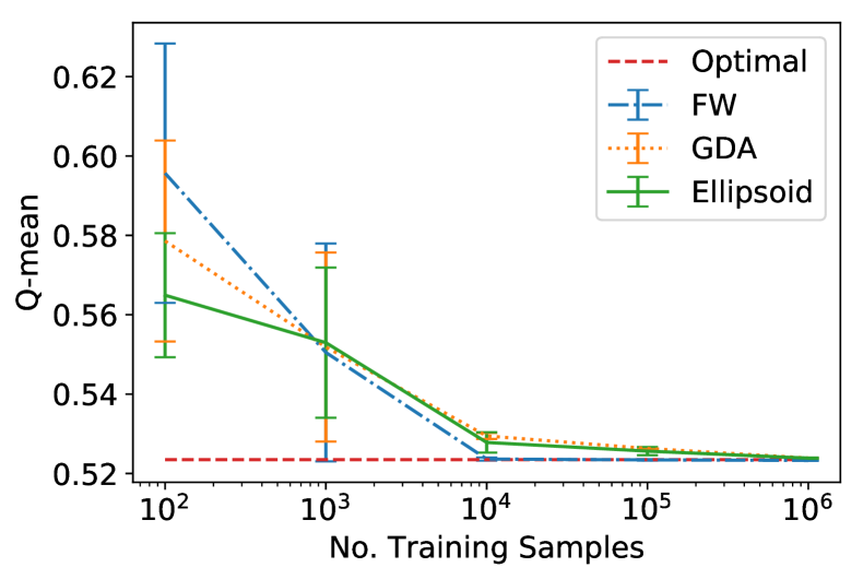
(a) Unconstrained

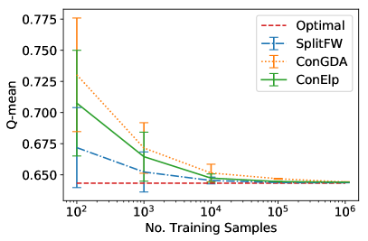
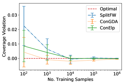
(b) Constrained

Figure 7: Convergence of the proposed algorithms on synthetic data to (a) the Bayes optimal classifier for of the Q-mean loss, and (b) the optimal-feasible classifier for the task of minimizing Q-mean loss subject to a coverage constraint, with the Q-mean loss shown on the left and the coverage constraint violation $\max_{i\in[3]}\big{|}\sum_{j}C_{ji}-\pi_{i}\big{|}-0.01$ shown on the right. The results are reported on the test set, and averaged over training with 5 random draws of the dataset.

8.3 Convergence to the Optimal Classifier

In our first set of experiments, we test the consistency behavior of the algorithms on a synthetic data set for which the Bayes optimal performance could be calculated. We use a 3-class synthetic data set with instances in ${\mathcal{X}}={\mathbb{R}}^{2}$ generated as follows: examples are chosen from class 1 with probability 0.85, from class 2 with probability 0.1 and from class 3 with probability 0.05; instances in the three classes are then drawn from multivariate Gaussian distributions with means $(1,1)^{\top}$, $(0,0)^{\top}$, and $(-1,-1)^{\top}$ respectively, and with the same covariance matrix $\big{[}\begin{smallmatrix}5&1\\ 1&5\end{smallmatrix}\big{]}$. The conditional-class probability function ${\boldsymbol{\eta}}:{\mathbb{R}}^{2}{\rightarrow}\Delta_{3}$ for this distribution is a softmax of linear functions, and can be computed in closed-form.

We first consider the unconstrained task of optimizing the Q-mean loss in Table 1, given by $\psi^{\text{QM}}({\mathbf{C}})=\Big{(}\frac{1}{n}\sum_{i}\left(1-\frac{C_{ii}}{\sum_{j}C_{ij}}\right)^{2}\Big{)}^{1/2}$. Note that this performance metric is a smooth convex function of ${\mathbf{C}}$, and can be optimized with any one of the proposed Frank-Wolfe, GDA or ellipsoid methods (Algorithms 1–3). Because the metric and the distribution satisfy the conditions of Proposition 9, and the Bayes-optimal classifier is of the form $h^{*}(x)=\operatorname{argmax}^{*}_{i\in[3]}w^{*}_{i}\,\eta_{i}(x)$, for some distribution-dependent coefficients $w^{*}_{i}\in{\mathbb{R}}$,. To compute the Bayes-optimal classifier, we run a brute-force grid search for $w^{*}_{i}$.

Our algorithms use the plug-in method in Algorithm 9 for the LMO subroutine. Specifically, they fit a linear logistic regression model $\widehat{{\boldsymbol{\eta}}}:{\mathbb{R}}^{2}{\rightarrow}\Delta_{3}$ to the training set, and iteratively learn a randomized combination of classifiers of the form $h(x)=\operatorname{argmax}^{*}_{i\in[3]}w_{i}\,\widehat{\eta}_{i}(x)$. In Figure 7(a), we plot the Q-mean loss for the classifier learned by the proposed algorithms, evaluated on a test set of $10^{6}$ examples, for different sizes of the training sample. In each case, we average the results over 5 random draws of the training sample. As seen, all three methods converge to the performance of the Bayes-optimal classifier.

We next consider the task of optimizing the Q-mean loss subject to a coverage constraint, requiring the proportion of predictions made for class $i$ to be (approximately) equal to the class prior $\pi_{i}$. Specifically, we constraint the max coverage deviation, $\max_{i\in[3]}\big{|}\sum_{j}C_{ji}-\pi_{i}\big{|}$ to be at most 0.01. This is a constrained problem with a convex smooth objective and a convex constraint in ${\mathbf{C}}$, and can be solved using the constrained counter-parts to the Frank-Wolfe, GDA and ellipsoid methods (Algorithm 5–7). Following Yang et al. (2020), we have that the optimal-feasible classifier for this problem is a randomized classifier of two classifiers $h^{1,*}(x)=\operatorname{argmax}^{*}_{i\in[3]}w^{1,*}_{i}\eta_{i}(x)$ and $h^{2,*}(x)=\operatorname{argmax}^{*}_{i\in[3]}w^{2,*}_{i}\eta_{i}(x)$, for distribution-dependent coefficients $w^{1,*}_{i}$ and $w^{2,*}_{i}$. We compute these coefficients and the optimal randomized combination via a brute-force grid search. Figure 7(b) plots the Q-mean loss and the constraint violation for the three algorithms. All of them can be seen to converge to the Q-mean of the optimal-feasible classifier and to zero constraint violation.

8.4 Performance on Unconstrained Problems

We next compare the proposed algorithms for unconstrained problems on five benchmark multiclass datasets: (i) Abalone, (ii) PageBlock, (iii) CovType, (iv) SatImage and (v) MACHO. The first four were obtained from the UCI Machine Learning repository (Frank and Asuncion, 2010). The fifth dataset pertains to the task of classifying celestial objects from the Massive Compact Halo Object (MACHO) catalog using photometric time series data (Alcock et al., 2000; Kim et al., 2011). Each celestial object is described by measurements from 6059 light curves, and is categorized either as one of seven celestial objects or as a miscellaneous category.

We consider two performance metrics from Table 1: (i) the H-mean metric $\psi^{\textup{{HM}}}({\mathbf{C}})=1\,-\,n\left({\sum_{i}\frac{\sum_{j}C_{ij}}{C_{ii}}}\right)^{-1}$ and (ii) the micro F-measure $\psi^{{\textup{{micro}}F_{1}}}({\mathbf{C}})=1\,-\,\frac{2\sum_{i\neq k}C_{ii}}{2-\sum_{i}C_{ki}-\sum_{i}C_{ik}}$, where $k\in[n]$ is a designated default class. The first metric is convex in ${\mathbf{C}}$, for which we compare the performances of the Frank-Wolfe, GDA, and ellipsoid algorithms (Algorithms 1–3); the second metric is ratio-of-linear in ${\mathbf{C}}$, and for this, we apply the bisection algorithm (Algorithm 4). Our algorithms use a plug-in based LMO with a linear logistic regression model used to estimate the conditional-class probabilities. We compare our methods with the 0-1 plug-in, balanced plug-in and TFCO baselines.

Table 6: Unconstrained optimization of the (convex) H-mean loss. Lower values are better. The results are averaged over 10 random train-test splits.

Dataset	Plugin [0-1]	Plugin (bal)	TFCO	FW	GDA	Ellipsoid
Abalone	$1.0\pm 0.0$	$0.890\pm 0.038$	$0.824\pm 0.018$	$\textbf{0.816}\pm\textbf{0.020}$	$0.818\pm 0.017$	$0.817\pm 0.019$
Pgblk	$0.416\pm 0.128$	$0.130\pm 0.034$	$0.200\pm 0.023$	$0.120\pm 0.028$	$0.130\pm 0.04$	$\textbf{0.110}\pm\textbf{0.025}$
MACHO	$0.210\pm 0.043$	$0.130\pm 0.015$	$0.143\pm 0.019$	$0.124\pm 0.017$	$\textbf{0.124}\pm\textbf{0.015}$	$0.125\pm 0.017$
SatImage	$0.279\pm 0.01$	$0.173\pm 0.008$	$\textbf{0.170}\pm\textbf{0.006}$	$0.171\pm 0.007$	$0.173\pm 0.008$	$\textbf{0.170}\pm\textbf{0.006}$
CovType	$1.0\pm 0.0$	$0.507\pm 0.001$	$0.469\pm 0.001$	$0.463\pm 0.001$	$0.463\pm 0.001$	$\textbf{0.461}\pm\textbf{0.001}$

Table 7: Unconstrained optimization of the (ratio-of-linear) micro $F_{1}$ loss. Lower values are better. The results are averaged over 10 random train-test splits.

Datasets	Plugin [0-1]	Plugin (bal)	TFCO	Bisection
Abalone	$0.713\pm 0.006$	$0.760\pm 0.004$	$0.728\pm 0.012$	$\mathbf{0.693\pm 0.006}$
Pgblk	$0.218\pm 0.012$	$0.441\pm 0.033$	$0.216\pm 0.018$	$\mathbf{0.211\pm 0.016}$
MACHO	$\textbf{0.089}\pm\textbf{0.005}$	$0.106\pm 0.007$	$0.110\pm 0.005$	$\mathbf{0.089\pm 0.005}$
SatImage	$\textbf{0.180}\pm\textbf{0.005}$	$0.185\pm 0.007$	$0.234\pm 0.003$	$\mathbf{0.180\pm 0.005}$
CovType	$0.548\pm 0.001$	$0.625\pm 0.003$	$0.486\pm 0.001$	$\mathbf{0.403\pm 0.001}$

The results of optimizing the two metrics are shown in Tables 6 and 7 respectively. As expected both the 0-1 and balanced plug-in classifiers are often seen to perform poorly on the H-mean and micro $F_{1}$ metrics. For example, on the Abalone and CovType dataset, the plug-in (0-1) yields a H-mean loss of 1 as it achieves high accuracies on the higher-frequency classes at the cost of yielding zero accuracy on one or more minority classes. In contrast, the proposed algorithms provide equitable performance across all classes, and are able to yield a much lower H-mean score. This demonstrates the advantage of using algorithms that directly optimize for the metric of interest. In most experiments, TFCO is seen to be a competitive baseline: with the H-mean metric, the proposed algorithms yields significantly better performance over this method on two of the five datasets, and with the micro $F_{1}$ metric it yields significantly better performance than TFCO on four of the five datasets . We stress that our algorithms are able to provide these gains despite TFCO using a more flexible class of randomized classifiers. In fact, with the MACHO dataset, TFCO can be seen to perform worse than our method as a result of over-fitting to the training set.

We also note that all the algorithms compared beat a trivial classifier that predicts all classes with equal probability (see Appendix B.2 for the performance of the trivial classifier on the different datasets with different metrics).

8.5 Performance on Constrained Problems

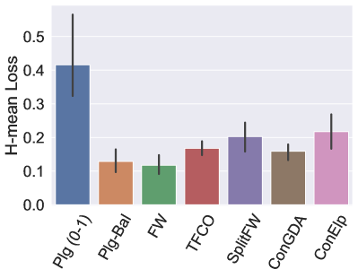
(a) PageBlock

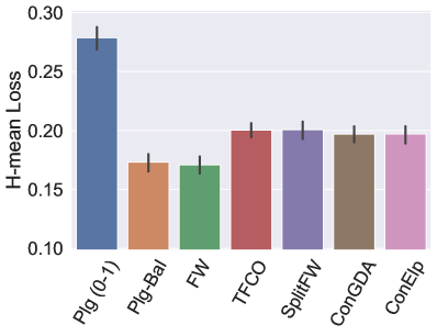
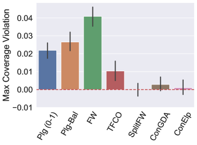
(b) SatImage

Figure 8: Optimizing the H-mean loss subject to the coverage constraint $\max_{i}|\sum_{j}C_{ji}\,-\,\pi_{i}|\leq 0.01$. The plots on the left show the H-mean loss on the test set and those on the right show the coverage violation $\max_{i}|\sum_{j}C_{ji}\,-\,\pi_{i}|-0.01$ on the test set. Lower H-mean value are better, and the constraint values need to be $\leq 0$. The results are averaged over 10 random train-test splits. The error bars indicate 95% confidence intervals.

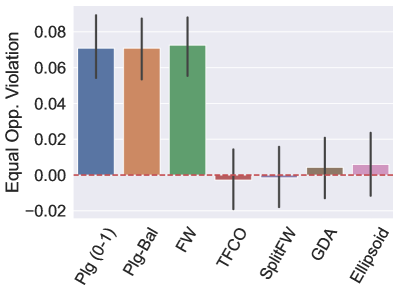
(a) COMPAS

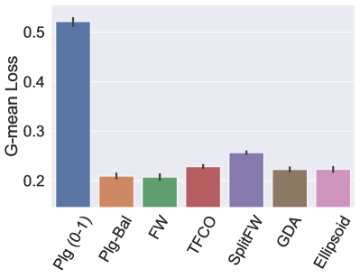
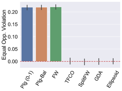
(b) Law School

Figure 9: Optimizing the G-mean loss subject to the equal-opportunity fairness constraint $\max_{a\in[m]}\big{|}\frac{1}{\mu_{a1}}C^{a}_{11}\,-\,\frac{1}{\pi_{1}}C_{11}\big{|}\leq 0.05$. The plots on the left show the G-mean loss on the test set and those on the right show the equal opportunity violation $\max_{a\in[m]}\big{|}\frac{1}{\mu_{a1}}C^{a}_{11}\,-\,\frac{1}{\pi_{1}}C_{11}\big{|}$ on the test set. Lower G-mean value are better, and the constraint violations need to be $\leq 0$. The results are averaged over 10 random train-test splits. The error bars indicate 95% confidence intervals.

Having showed the efficacy of our algorithms on unconstrained problems, we move to constrained problems. The first task we consider is to minimize the H-mean loss subject to coverage constraint requiring the proportion of predictions for each class $i$ to match the class prior $\pi$. Specifically, we require the maximum coverage violation over the $n$ classes $\max_{i\in[n]}|\sum_{j}C_{ji}\,-\,\pi_{i}|$ to be at most 0.01. In Figure 8, we report both the H-mean and the maximum coverage violation for the three proposed constrained learning algorithms (Algorithms 5–7) for this problem (see Appendix B.3 for additional results). For comparison, we also report the performance of the 0-1 plug-in, balanced plug-in, and TFCO baselines, as well as the unconstrained Frank-Wolfe (FW) method, which seeks to optimize only the H-mean ignoring the constraint. We find that all three algorithms satisfy the constraint on the training set, but occasionally incur some violations on the test set. In contrast, all baselines expect TFCO fail to satisfy the constraint. On SatImage, TFCO satisfies the constraint on the training set, but fails to satisfy it on the test set, while the proposed methods incur much lower test violations. This is also the case with MACHO, where TFCO incurs lower constraint violation and loss value on the training set, but compared to our methods is worse of on both metrics on the test set. The reason our methods are less prone to over-fitting is because they use a plug-in based LMO that post-shifts a pre-trained class-probability estimator, and therefore have fewer parameters to optimize when compared to TFCO.

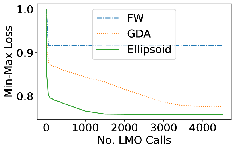
(a) Abalone (Train)

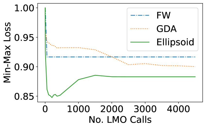
(b) Abalone (Test)

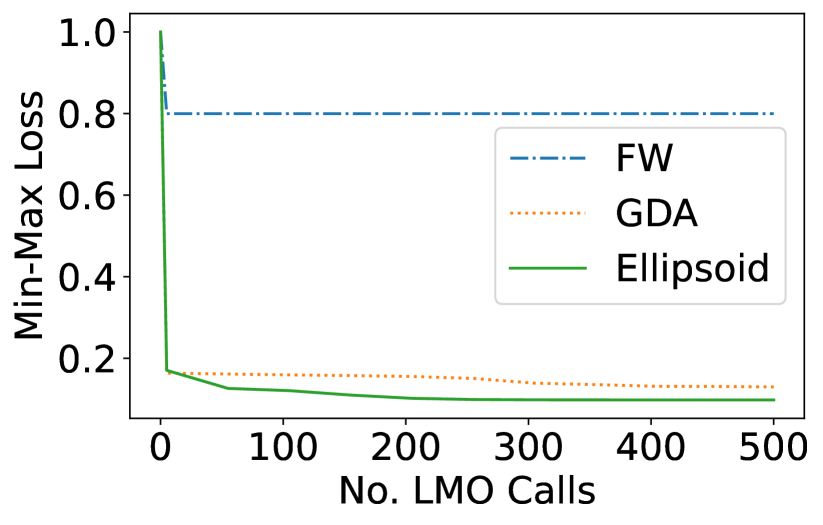
(c) PageBlock (Train)

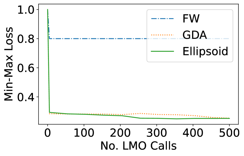
(d) PageBlock (Test)

Figure 10: Optimizing the Min-max loss: Comparison of performance of the Frank-Wolfe, GDA and ellipsoid methods as a function of the number of LMO calls. Lower values are better. Because the min-max loss is non-smooth, Frank-Wolfe is seen to converge to a sub-optimal classifier.

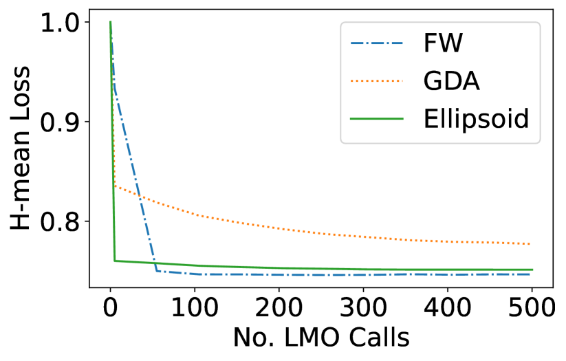
(a) Abalone (Train)

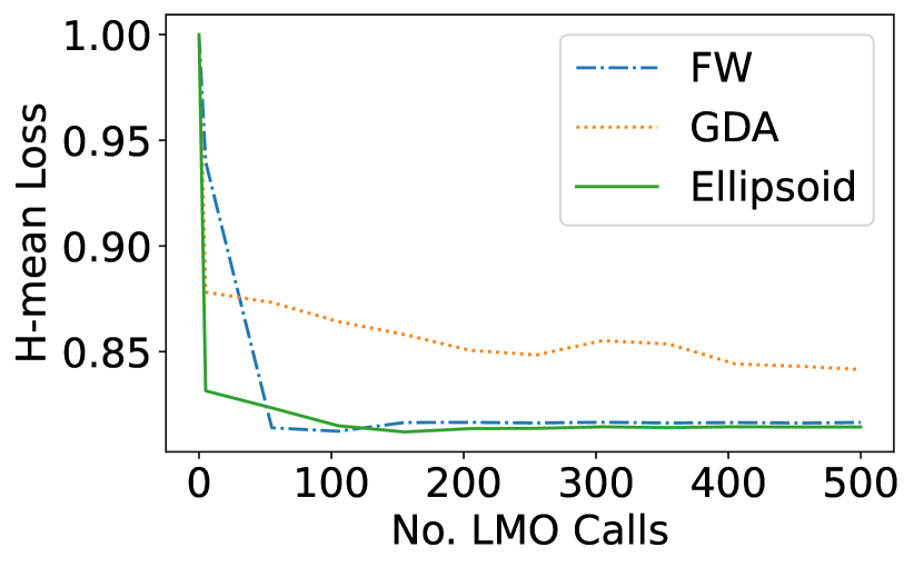
(b) Abalone (Test)

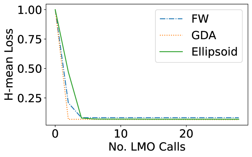
(c) PageBlock (Train)

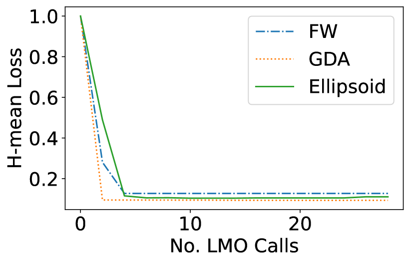
(d) PageBlock (Test)

Figure 11: Optimizing the H-mean loss: Comparison of performance of the Frank-Wolfe, GDA and ellipsoid methods as a function of the number of LMO calls. Lower values are better.

Our second task seeks to impose fairness constraints on benchmark fair classification datasets containing protected group information. These include: (1) COMPAS, where the goal is to predict recidivism with gender as the protected attribute (Angwin et al., 2016); (2) Communities & Crime, where the goal is to predict if a community in the US has a crime rate above the $70$th percentile (Frank and Asuncion, 2010), and we consider communities having a black population above the $50$th percentile as protected (Kearns et al., 2018); (3) Law School, where the task is to predict whether a law school student will pass the bar exam, with race (black or other) as the protected attribute (Wightman, 1998); (4) Adult, where the task is to predict if a person’s income exceeds 50K/year, with gender as the protected attribute (Frank and Asuncion, 2010); (5) Default, where the task is to predict if a credit card user defaulted on a payment, with gender as the protected attribute (Frank and Asuncion, 2010). While these are all binary-labelled datasets, because we wish to evaluate performance separately on the individual protected groups, the number of threshold parameters needed to learn a naïve plug-in classifier like the one described in Section 3.3 would grow exponentially with the number of groups, making the algorithms proposed in this paper desirable even in these multi-group settings.

The specific optimization goal is to minimize the G-mean loss $\psi^{\textup{{GM}}}({\mathbf{C}})=1\,-\,\big{(}\prod_{i}\frac{C_{ii}}{\sum_{j}C_{ij}}\big{)}^{1/n}$ subject to an equal opportunity constraint $\max_{a\in[m]}\big{|}\frac{1}{\mu_{a1}}C^{a}_{11}\,-\,\frac{1}{\pi_{1}}C_{11}\big{|}\leq 0.05$, requiring the true positive rates for different protected groups to be similar. The plots in Figure 9 presents the results for the three proposed algorithms relevant to this problem, and show both the G-mean loss and the equal opportunity violation (more results in Appendix B.3). In addition to the 0-1 plug-in, balanced plug-in and TFCO baselines, we include an unconstrained Frank-Wolfe (FW) method which seeks to minimize only the G-mean ignoring the constraint. All these methods incur large constrained violations. The objectives are largely comparable for the three proposed methods, except on LawSchool, where SplitFW yields a higher loss. The constraint violations for our methods are comparable to or lower than TFCO, with TFCO failing to satisfy the constraint on Crimes as a result of over-fitting to the training set.

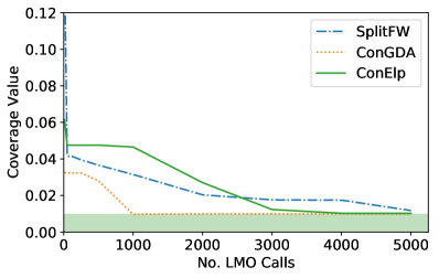
(a) Abalone (Train)

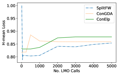
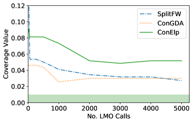
(b) Abalone (Test)

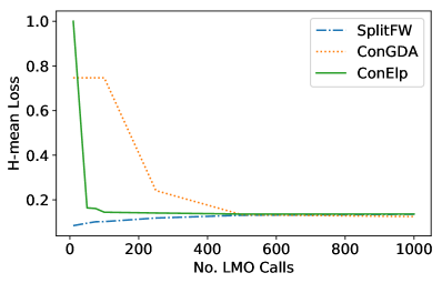
(c) PageBlock (Train)

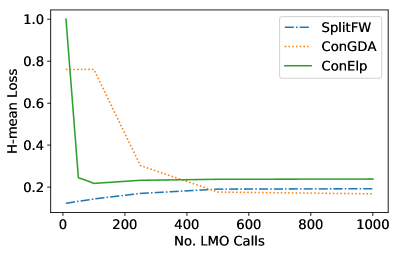
(d) PageBlock (Test)

Figure 12: Optimizing H-mean subject to coverage constraint: Comparison of performance of SplitFW, ConGDA and ConEllipsoid algorithms as a function of the number of LMO calls. Lower H-mean values are better. Green shaded region denotes coverage values that satisfy the constraints.

8.6 Practical Guidance on Algorithm Choice

Of the three types of algorithms we have proposed for convex metrics $\psi$, the choice of the algorithm to use in an application would depend on three factors: the smoothness of the metric, the presence of constraints, and the dimension of the problem. In Figure 10, we consider the task of optimizing the min-max metric $\psi^{\text{MM}}({\mathbf{C}})=\max_{i}\left(1-\frac{C_{ii}}{\sum_{j}C_{ij}}\right)$, a non-smooth function of ${\mathbf{C}}$, and plot the performance of the three algorithms (with a plug-in based LMO) on the training and test sets as a function of the number of calls to the LMO. Since the objective for this unconstrained problem does not satisfy the smoothness property required by the Frank-Wolfe algorithm, as expected, it fairs poorly even with a large number of LMO calls. The ellipsoid algorithm is often seen to exhibit faster convergence than GDA on the training set, but there isn’t a clear winner on the test set. In Figure 10, we repeat the experiment with the smooth H-mean metric, and find that Frank-Wolfe algorithm does converge to a similar performance as the other methods, and is in fact the fastest to do so on the 12-class Abalone dataset. Moreover unlike the GDA, the Frank-Wolfe algorithm has no additional hyper-parameters to tune and is therefore an attractive option for smooth convex metrics.

On the other hand, when it comes to constrained problems, we find the (constrained) GDA algorithm to exhibit the fastest convergence. In this case, the (constrained) ellipsoid algorithm may take longer to converge to the optimal-feasible solution, particularly when the number of classes is high (as seen from the strong dependence on dimension its convergence rate has in Theorem 18). For example, this evident with the 12-class Abalone dataset in Figure 12(a)–(b), where we seek to maximize the H-mean loss subject to the coverage constraint described in Section 8.5, and find the GDA algorithm to converge the fastest to a feasible classifier. In contrast, the (constrained) ellipsoid algorithm exhibits the fastest convergence on the smaller 5-class PageBlock dataset (although it yields slightly worse H-mean values than the other methods on the test set). See Appendix B.3 for additional experimental results.

Overall, we prescribe using the ellipsoid algorithm (or its constrained counterpart) for problems with a small number of classes, the FrankWolfe algorithm if the metric is smooth and there are no constraints, and the GDA algorithm (or its constrained counterpart) for all other scenarios.

Table 8: Comparison of the plug-in and weighted logistic regression (WLR) based LMOs on the task of optimizing the (convex) H-mean loss. The number of iterations, i.e. calls to the LMO, is fixed at 20. Lower values are better. The results are averaged over 10 random train-test splits.

Data	FW		GDA		Ellipsoid
	Plugin	WLR	Plugin	WLR	Plugin	WLR
Aba	$0.797\pm 0.008$	$\textbf{0.791}\pm\textbf{0.004}$	$0.892\pm 0.038$	$\textbf{0.838}\pm\textbf{0.017}$	$0.833\pm 0.038$	$0.833\pm 0.038$
PgB	$0.13\pm 0.038$	$\textbf{0.084}\pm\textbf{0.015}$	$0.129\pm 0.034$	$\textbf{0.083}\pm\textbf{0.018}$	$0.105\pm 0.019$	$\textbf{0.080}\pm\textbf{0.017}$
MAC	$\textbf{0.125}\pm\textbf{0.01}7$	$0.245\pm 0.027$	$\textbf{0.124}\pm\textbf{0.015}$	$0.206\pm 0.028$	$\textbf{0.122}\pm\textbf{0.015}$	$0.247\pm 0.027$
Sat	$0.174\pm 0.007$	$\textbf{0.171}\pm\textbf{0.007}$	$\textbf{0.173}\pm\textbf{0.008}$	$0.176\pm 0.006$	$0.168\pm 0.006$	$\textbf{0.167}\pm\textbf{0.006}$
Cov	$0.468\pm 0.001$	$\textbf{0.453}\pm\textbf{0.001}$	$0.488\pm 0.001$	$\textbf{0.453}\pm\textbf{0.001}$	$0.463\pm 0.001$	$\textbf{0.447}\pm\textbf{0.001}$

8.7 Choice of LMO: Plug-in vs. Weighted Logistic Regression

In previous experiments, we have seen that the proposed algorithms were less prone to over-fitting because of the use of a plug-in based LMO that post-fit a small number of parameters to a pre-trained model. We now compare the performance of these algorithms with an LMO that re-trains a classifier from scratch each time it is called. Specifically, we repeat the H-mean optimization task from Section 8.4, with weighted (linear) logistic regression as the LMO. For a given (diagonal) loss matrix ${\mathbf{L}}$, this LMO learns a classifier by optimizing a weighted logistic loss, where the per-class weights are set to be the diagonal entries of ${\mathbf{L}}$. Note that such a weighted surrogate loss is calibrated for ${\mathbf{L}}$ (Tewari and Bartlett, 2007). Unlike the simple plug-in LMO, each call to weighted logistic regression can be expensive; hence it is important that we are able to limit the number of calls to it.

In Table 8, we present results comparing performance of the Frank-Wolfe, GDA and ellipsoid algorithms with the plug-in and weighted logistic regression LMOs when run for 20 iterations. Appendix B.3 contains results of these experiments when the algorithms are allowed 100 iterations. The performance with the two LMOs are comparable on Abalone and SatImage. On PageBlocks and CovType, weighted logistic regression has a moderate to significant advantage. Interestingly, on MACHO, the plug-in based LMO, despite learning from a less flexible hypothesis class (post-hoc adjustments to a fixed model), is substantially better. This is because weighted logistic regression over-fits to the training set in this case.

Overall, we find that an LMO such as weighted logistic regression, while being computationally expensive, does sometimes provide metric gains over a less-flexible plug-in type approach. However, this method can be prone to over-fitting because of its added flexibility.

8.8 Case Study: Image Classification with Imbalance and Label Noise

As case studies, we demonstrate two natural workflows our algorithms in (i) tackling label imbalance in CIFAR-55 and (ii) mitigating label noise in a noisy version of CIFAR-10.

8.8.1 Class Imbalance with Large Number of Classes

One of the undesirable effects of learning with a class-imbalanced dataset is that the learned classifier tends to over-predict classes that are more prevalent and under-predict classes that are rare. We consider two approaches to avoid this problem: minimizing a loss such as the H-mean that emphasizes equal performance across all classes, and constraining the proportions of predictions the classifier makes for each class to match the true prevalence of the class.

For this experiment, we use the CIFAR-100 dataset (Krizhevsky, 2009), which contains images labelled with one of 100 classes. We create an imbalanced 55-class dataset by merging 50 classes in CIFAR-100 into 5 “super-classes” (see Appendix B.2 for details), and leaving the rest of the classes untouched. In the resulting class distribution, 5 of the classes are 10 times more prevalent than the remaining 50. All our methods use a plug-in based LMO which uses a pre-trained class probability estimator. We train a ResNet-50 model for the class probability estimator, using SGD to minimize the standard cross-entropy loss. We use a batch size of 64, a base learning rate of 0.01 (with a warm-up cosine schedule), and a momentum of 0.9. We apply a weight decay of 0.01 and train for 39 epochs.

In Table 9, we analyze the performance of a ResNet-50 model trained with the standard cross-entropy loss (Plugin [0-1]), where the class that receives the highest estimated probability is predicted as the output label, and report its 0-1 loss, its H-mean loss, and the deviation of its class prediction rates from the prior probabilities, i.e. its maximum coverage violation: $\max_{i\in[n]}|\sum_{j}C_{ji}\,-\,\pi_{i}|$. We find that naïvely optimizing for the 0-1 loss yields a high coverage violation. Moreover, it yields high accuracies on the 5 super-classes, at the cost of a much lower accuracy on the 50 minority classes, resulting in a high H-mean loss. To emphasize better performance on the minority classes, we train classifiers to minimize the H-mean loss (FW [H-mean]), and minimize the 0-1 loss subject to the maximum coverage violation being within a tolerance of 0.01 (SplitFW [0-1]). We also consider a combination of both, i.e. minimizing the H-mean loss subject to the maximum coverage violation being within 0.01 (SplitFW [H-mean]). It can be seen that all three algorithms do only slightly worse than the Plugin [0-1] baseline in terms of 0-1 loss, but do significantly better in terms of both the H-mean loss and the coverage violation.

Table 9: Results on CIFAR-55 imbalanced dataset. The train and test sets are imbalanced, with 5 classes being 10 times larger in size than the remaining 50 classes. We report the 0-1 loss, the H-mean loss, and the coverage violation $\max_{i\in[n]}|\sum_{j}C_{ji}\,-\,\pi_{i}|-0.01$. Lower values are better.

Method	Train (Imbalanced)			Test (Imbalanced)
	0-1	H-mean	Violation	0-1	H-mean	Violation
Plugin [0-1]	0.278	0.457	0.030	0.437	0.709	0.045
FW [H-mean]	0.307	0.323	0.026	0.481	0.564	0.029
SplitFW [0-1]	0.279	0.391	0.000	0.436	0.636	0.007
SplitFW [H-mean]	0.279	0.342	0.000	0.448	0.595	0.000

8.8.2 Class Imbalance with Label Noise

Our next experiment demonstrates how label noise can be mitigating by imposing coverage constraints on the classifier. We use a class-imbalanced version of the CIFAR-10 dataset (Krizhevsky, 2009), where we sub-sample images from classes 1 to 5 by a factor of 10, with the resulting class priors are given by $\pi_{y}=\frac{2}{110}$ when $y\in\{1,2,3,4,5\}$ and $\pi_{y}=\frac{2}{11}$ otherwise. Our algorithms assume the knowledge of $\pi$. In addition to class imbalance, very often one has to work with noisy training labels to building a classifier that performs well on uncorrupted test data. We simulate this scenario by adding a label noise corruption to the training data, which is chosen such that classes 1 to 9 are left undisturbed, and the labels of images from class 10 are randomly chosen from 1 to 10. This effectively mimics a crowd-sourced label collection with 9 easy labels, and one difficult or incomprehensible label. Our algorithms do not have knowledge of this corruption.

Equipped with the knowledge of the class priors $\pi$, we propose constraining the proportion of predictions made for each class to match the priors $\pi$. While this is not necessarily equivalent to training the classifier with uncorrupted labels, we expect that these additional coverage constraints will dampen the effect of the noisy labels. As with the previous experiment, we evaluate the classifier on two criteria: (i) how well it performs on the (balanced) H-mean metric on the test data, and (ii) how well the class prediction rates match the priors $\pi$ on the test data. Our framework can be applied to this problem by minimizing the H-mean error on the corrupted training dataset, subject to a coverage constraint on the classifier forcing it to predict classes at a rate that matches $\pi$.

In addition to a ResNet model baseline that optimizes the cross-entropy loss (Plugin [0-1]), we include the state-of-the-art method of Patrini et al. (2017), which uses the predictions from Plugin [0-1] on the training data to compute an estimate of the label noise transition matrix, and re-trains the classifier with a (forward) correction computation applied to the loss (Noise Correction [Estimate]). For completeness, we also include an idealized version of this method, where the “exact” noise transition matrix is used for the forward correction (Noise Correction [Exact]). While this baseline is unrealistic, it provides us with an estimate best possible 0-1 loss achievable for this problem.

We provide the result of this experiment in Table 10, where FW [H-mean] corresponds to a classifier that minimizes the H-mean loss on the corrupted training dataset, and SplitFW [0-1] (resp. SplitFW [H-mean]), correspond to a classifier that minimizes the 0-1 loss (resp. H-mean loss) on the corrupted training dataset, while enforcing the coverage constraint to a tolerance of $0.01$. All three methods use the same underlying class probability model as Plugin [0-1]. It is seen that only SplitFW [0-1] and SplitFW [H-mean] achieve low coverage violations on the test set, and are still only moderately worse than the idealized Noise Correction [Exact] method in terms of their respective objective metrics. The FW [H-mean] algorithm achieves the best H-mean on clean test data despite being trained on the corrupted training labels.

Table 10: Results on imbalanced CIFAR-10 dataset with label noise. The train set is imbalanced and has label noise, while the test set is imbalanced but clean. We report the 0-1 loss, the H-mean loss, and the coverage violation $\max_{i\in[n]}|\sum_{j}C_{ji}\,-\,\pi_{i}|-0.01$. Lower values are better.

Method	Train (Flipped)			Test (Imbalanced)
	0-1	H-mean	Violation	0-1	H-mean	Violation
Plugin [0-1]	0.266	0.896	0.170	0.332	0.899	0.169
Noise Correction [Estimate]	0.174	0.370	0.054	0.179	0.430	0.055
FW [H-mean]	0.348	0.481	0.072	0.329	0.396	0.076
SplitFW [0-1]	0.272	0.609	0.001	0.196	0.610	0.004
SplitFW [H-mean]	0.292	0.523	0.003	0.221	0.471	0.003
Noise Correction [Exact]	0.196	0.394	0.022	0.151	0.358	0.018

9 Conclusions

We have developed a framework for designing consistent and efficient algorithms for multiclass performance metrics and constraints that are general functions of the confusion matrix. As instantiations of this framework, we provided four algorithms for optimizing unconstrained metrics, and four analogous counterparts for solving constrained learning problems. In each case, we have shown convergence guarantees for the algorithms under different assumptions on the performance metrics and constraints.

Our key idea was to reduce the complex learning problem into a sequence of linear minimization problems, for which we recommended an efficient plug-in based approach that applies a post-hoc transformations to a pre-trained class probability model. The results of these linear minimization problems are then combined to return a final classifier. One of the main challenges in instantiating this idea was to identify optimization algorithms for different problem settings that only required access to a linear minimization oracle (LMO).

We also presented extensive experiments on a variety of multiclass and fairness datasets and demonstrated that the proposed algorithms (despite being limited to performing adjustments to a fixed model) are competitive or better than the state-of-the-art TFCO approach (Cotter et al., 2019b) which works with a more flexible hypothesis class. We additionally provided precise guidance for which of the proposed algorithms are best suited for a given multiclass problem, and highlighted scenarios where one might want to use a more expensive LMO that trains a new classifier from scratch at each iteration.

Over the years, the conference versions of this paper have attracted several follow-up works, which have adapted our ideas to optimizing multiclass extensions of the F-measure (Pan et al., 2016), to balancing accuracy with fairness objectives (Alabi et al., 2018), to eliciting multi-class performance metrics (Hiranandani et al., 2019), to training classifiers to optimize more general multi-output classification metrics (Wang et al., 2019), to imposing fairness constraints with overlapping protected groups (Yang et al., 2020), and to optimizing black-box evaluation metrics Hiranandani et al. (2021).

A number of follow-up directions arise from the proposed framework. First, it would interesting to derive lower bounds on the number of calls to the LMO needed under different assumptions on the performance metrics and constraints.

Second, while the optimality (and feasibility) gap for most of our proposed algorithms depend linearly on the LMO approximation errors $\rho$ and $\rho^{\prime}$, the split Frank-Wolfe method (Algorithm 5 alone has a square-root dependence on these parameters. Are these dependencies on the LMO errors optimal or simply artifacts of the analysis?

Third, for algorithms where the convergence rates have a linear (or quadratic) dependence on the dimension of the problem $d$ (which is typically the same order as the number of classes), how does one extend our framework to handle problems with an extremely large number classes (perhaps under additional structural assumptions on the classes, akin to Ramaswamy et al. (2015)) and problems with an extremely large number of constraints (Narasimhan et al., 2020)?

Fourth, our experiments in Section 8.7 show that in some applications, using a flexible LMO that trains a classifier from scratch can yield significant gains over a plug-in based LMO, but this however comes at the cost of added computational time. Can one devise an intermediate approach, where each call to the LMO only needs to run a constant number of optimization steps on a surrogate loss (akin to the TFCO baseline of Cotter et al. (2019b)), while still guaranteeing that the outer algorithm provably convergences to the optimal (feasible) classifier?

Finally, except for the bisection method, all the algorithms we propose rely on the use of a randomized classifier. In some applications, deploying a randomized classifier can be undesirable for ethical reasons or because of the engineering difficulties it poses. In these scenarios, one could approximate the learned randomized classifier with a deterministic classifier using, for example, the approach of Cotter et al. (2019). Understanding the loss in performance and constraint satisfaction as a result of such de-randomization procedures is an interesting direction for future work.

Table 11: Table of notations.

Notation	Description
$n$	Number of classes
$N$	Number of training examples
$m$	Number of protected groups
$K$	Number of constraints
$d$	Dimension of the vector representation for the confusion matrix
$T$	Number of iterations for the proposed iterative algorithms
$i,j$	Indices over $n$ classes
$a$	Index over $m$ protected groups
$k$	Index over $K$ constraints
$t$	Index over $T$ iterations
$\ell$	Index over $N$ training instances
${\mathbf{C}}$	$n\times n$ Confusion matrix, or an equivalent vector representation of dimension $d=n^{2}$
${\mathbf{L}}$	$n\times n$ Loss matrix, or an equivalent vector representation of dimension $d=n^{2}$
${\mathcal{C}}$	Set of achievable confusion matrices, represented by vectors of dimension $d=n^{2}$
$S$	Training sample with $N$ instances

A Proofs

A.1 Proof of Proposition 8 (Bayes-optimal Classifier for Ratio-of-linear $\psi$)

Proposition ((Restated) Bayes optimal classifier for ratio-of-linear $\psi$).

Let the performance measure $\psi:[0,1]^{d}{\rightarrow}{\mathbb{R}}_{+}$ in OP1 be of the form $\psi({\mathbf{C}})=\frac{\langle{\mathbf{A}},{\mathbf{C}}\rangle}{\langle{\mathbf{B}},{\mathbf{C}}\rangle}$ for some ${\mathbf{A}},{\mathbf{B}}\in{\mathbb{R}}^{d}$ with $\langle{\mathbf{B}},{\mathbf{C}}\rangle>0~{}\forall{\mathbf{C}}\in{\mathcal{C}}$. Let $t^{*}=\inf_{{\mathbf{C}}\in{\mathcal{C}}}\psi({\mathbf{C}})$ and ${\mathbf{L}}^{*}={\mathbf{A}}-t^{*}{\mathbf{B}}$. Then any classifier that is optimal for the linear metric $\langle{\mathbf{L}}^{*},{\mathbf{C}}\rangle$ is also optimal for OP1.

We will find the following lemma useful in the proof of the proposition.

Lemma 25.

Let $\psi:[0,1]^{d}{\rightarrow}{\mathbb{R}}_{+}$ be such that $\psi({\mathbf{C}})=\frac{\langle{\mathbf{A}},{\mathbf{C}}\rangle}{\langle{\mathbf{B}},{\mathbf{C}}\rangle},$ for some matrices ${\mathbf{A}},{\mathbf{B}}\in{\mathbb{R}}^{d}$ with $\langle{\mathbf{B}},{\mathbf{C}}\rangle>0$ for all ${\mathbf{C}}\in{\mathcal{C}}$. Let $t^{*}=\inf_{{\mathbf{C}}\in{\mathcal{C}}}\psi({\mathbf{C}})$. Then $\inf_{{\mathbf{C}}\in{\mathcal{C}}}\langle{\mathbf{A}}-t^{*}{\mathbf{B}},{\mathbf{C}}\rangle=0.$

Proof.

Define $\varphi:{\mathbb{R}}{\rightarrow}{\mathbb{R}}$ as $\varphi(t)=\inf_{{\mathbf{C}}\in{\mathcal{C}}}\langle{\mathbf{A}}-t{\mathbf{B}},{\mathbf{C}}\rangle.$ It is easy to see that $\varphi$ (being a point-wise supremum of linear functions) is convex, and hence a continuous function over ${\mathbb{R}}$. Let $t^{*}=\inf_{{\mathbf{C}}\in{\mathcal{C}}}\psi({\mathbf{C}})$. We then have for all ${\mathbf{C}}\in{\mathcal{C}}$,

$$\frac{\langle{\mathbf{A}},{\mathbf{C}}\rangle}{\langle{\mathbf{B}},{\mathbf{C}}\rangle}\,\geq\,t^{*}~{}~{}~{}\text{or equivalently}~{}~{}~{}\varphi(t^{*})\,=\,\langle{\mathbf{A}}-t^{*}{\mathbf{B}},{\mathbf{C}}\rangle\,\geq\,0.$$

Thus

$$\varphi(t^{*})=\sup_{{\mathbf{C}}\in{\mathcal{C}}}\langle{\mathbf{A}}-t^{*}{\mathbf{B}},{\mathbf{C}}\rangle\geq 0\;.$$ (10)

Also, by continuity of $\frac{\langle{\mathbf{A}},{\mathbf{C}}\rangle}{\langle{\mathbf{B}},{\mathbf{C}}\rangle}$ in ${\mathbf{C}}$, for any $t<t^{*}$, there exists ${\mathbf{C}}\in{\mathcal{C}}$ such that

$$\frac{\langle{\mathbf{A}},{\mathbf{C}}\rangle}{\langle{\mathbf{B}},{\mathbf{C}}\rangle}\,>\,t~{}~{}~{}\text{or equivalently}~{}~{}~{}\varphi(t)\,=\,\langle{\mathbf{A}}-t{\mathbf{B}},{\mathbf{C}}\rangle\,<\,0.$$

Thus for all $t<t^{*}$,

$$\varphi(t)=\inf_{{\mathbf{C}}\in{\mathcal{C}}}\langle{\mathbf{A}}-t{\mathbf{B}},{\mathbf{C}}\rangle<0\;.$$

Next, by continuity of $\varphi$, for any monotonically increasing sequence of real numbers $\{t_{i}\}_{i=1}^{\infty}$ converging to $t^{*}$, we have that $\varphi(t_{i})$ converges to $\varphi(t^{*})$; since for each $t_{i}$ in this sequence $\varphi(t_{i})<0$, at the $t^{*}$, we have that $\varphi(t^{*})\geq 0$. Along with (10), this gives us

$$\inf_{{\mathbf{C}}\in{\mathcal{C}}}\langle{\mathbf{A}}-t^{*}{\mathbf{B}},{\mathbf{C}}\rangle=\varphi(t^{*})=0,$$

as desired. ∎

We are now ready to prove Proposition 8.

Proof of Proposition 8.

Let ${h}^{*}:{\mathcal{X}}{\rightarrow}\Delta_{n}$ be a classifier that is optimal for ${\mathbf{L}}^{*}={\mathbf{A}}-t^{*}{\mathbf{B}}$, i.e.,

$$\langle{\mathbf{A}}-t^{*}{\mathbf{B}},{\mathbf{C}}[{h}^{*}]\rangle\,=\,\inf_{{\mathbf{C}}\in{\mathcal{C}}}\langle{\mathbf{A}}-t^{*}{\mathbf{B}},{\mathbf{C}}\rangle.$$

Note from Lemma 25 that $\langle{\mathbf{A}}-t^{*}{\mathbf{B}},{\mathbf{C}}[{h}^{*}]\rangle=0$. Hence,

$$\frac{\langle{\mathbf{A}},{\mathbf{C}}[{h}^{*}]\rangle}{\langle{\mathbf{B}},{\mathbf{C}}[{h}^{*}]\rangle}\,=\,t^{*},\text{or equivalently},~{}~{}~{}~{}\psi({\mathbf{C}}[{h}^{*}])\,=\,\inf_{{\mathbf{C}}\in{\mathcal{C}}}\psi({\mathbf{C}}),$$

which shows that $h^{*}$ is also $\psi$-optimal. ∎

A.2 Proof of Proposition 9 (Bayes-optimal Classifier for Monotonic $\psi$)

Proposition ((Restated) Bayes-optimal classifier for monotonic $\psi$).

Let the performance measure $\psi:[0,1]^{d}{\rightarrow}{\mathbb{R}}_{+}$ in OP1 be differentiable and bounded, and be monotonically decreasing in $C_{ii}$ for each $i$ and non-decreasing in $C_{ij}$ for all $i,j$. Let ${\boldsymbol{\eta}}(X)$ be a continuous random vector. Then there exists a loss matrix ${\mathbf{L}}^{*}$ (which depends on $\psi$ and $D$) such that any classifier that is optimal for the linear metric given by ${\mathbf{L}}^{*}$ is also optimal for OP1.

Let $\overline{{\mathcal{C}}}$ denote the closure of ${\mathcal{C}}$. We will find the following lemma crucial to our proof.

Lemma 26.

Let $\eta(X)$ be a continuous random vector. Let ${\mathbf{L}}\in{\mathbb{R}}^{d}$ be such that no two columns are identical. Then,

$$\operatorname{argmin}_{{\mathbf{C}}\in\overline{{\mathcal{C}}}}\,\langle{\mathbf{L}},{\mathbf{C}}\rangle\,=\,\operatorname{argmin}_{{\mathbf{C}}\in{\mathcal{C}}}\langle{\mathbf{L}},{\mathbf{C}}\rangle.$$

Moreover, the above set is a singleton.

The proof for the lemma is highly technical and can be found in the conference version of the paper, specifically Lemma 12 in Narasimhan et al. (2015b).

Proof of Proposition 9.

Let ${\mathbf{C}}^{*}=\operatorname{argmin}_{{\mathbf{C}}\in\overline{{\mathcal{C}}}}\psi({\mathbf{C}})$. Such a ${\mathbf{C}}^{*}$ always exists by compactness of $\overline{{\mathcal{C}}}$ and continuity of $\psi$. By first order optimality, and convexity of $\overline{{\mathcal{C}}}$, we have that for all ${\mathbf{C}}\in\overline{{\mathcal{C}}}$

$$\langle\nabla\psi({\mathbf{C}}^{*}),{\mathbf{C}}^{*}\rangle\leq\langle\nabla\psi({\mathbf{C}}^{*}),{\mathbf{C}}\rangle\;.$$

For ${\mathbf{L}}^{*}=\nabla\psi({\mathbf{C}}^{*})$, we have that ${\mathbf{C}}^{*}\in\operatorname{argmin}_{{\mathbf{C}}\in\overline{{\mathcal{C}}}}\langle{\mathbf{L}}^{*},{\mathbf{C}}\rangle.$

Due to the monotonicity condition on $\psi$ the diagonal elements of its gradient $\nabla\psi({\mathbf{C}}^{*})$ are positive, and the off-diagonal elements are non-positive, and hence no two columns of ${\mathbf{L}}^{*}$ are identical. Thus by a direct application of Lemma 26, we have that ${\mathbf{C}}^{*}\in{\mathcal{C}}$, and moreover ${\mathbf{C}}^{*}$ is the unique minimizer of $\langle{\mathbf{L}}^{*},{\mathbf{C}}\rangle$ over all ${\mathbf{C}}\in{\mathcal{C}}$. ∎

A.3 Proof of Proposition 10 (Bayes-optimal Classifier for Continuous $\psi,\phi_{1},\ldots,\phi_{K}$)

Proposition (Bayes optimal classifier for continuous $\psi,\phi_{1},\ldots,\phi_{K}$).

Let the performance measure $\psi:[0,1]^{d}{\rightarrow}{\mathbb{R}}_{+}$ and the constraint functions $\phi_{1},\ldots,\phi_{K}:[0,1]^{d}{\rightarrow}{\mathbb{R}}$ in OP2 be continuous and bounded. Then there exists $d+1$ loss matrices ${\mathbf{L}}^{*}_{1},{\mathbf{L}}^{*}_{2},\ldots,{\mathbf{L}}^{*}_{d+1}$ (which can depend on $\psi,\phi_{k}$’s and $D$) such that an optimal classifier for OP2 can be expressed as a randomized combination of the deterministic classifiers $h_{1},h_{2},\ldots,h_{d+1}$, where $h_{i}$ is optimal for the linear metric given by ${\mathbf{L}}^{*}_{i}$.

Proof.

We first note that ${\mathcal{C}}$ is a compact set, and as a result there exists an optimal-feasible solution ${\mathbf{C}}^{*}$ for OP2 in ${\mathcal{C}}$. It is straightforward to see that ${\mathcal{C}}$ is bounded. To see that ${\mathcal{C}}$ is closed, note that from Proposition 5, any linear function over ${\mathcal{C}}$ is minimized by some confusion matrix in ${\mathcal{C}}$. Since every extreme point is a unique minimizer of a linear function in ${\mathcal{C}}$, every extreme point of ${\mathcal{C}}$ is also in ${\mathcal{C}}$. It follows that all convex combinations of the extreme points of ${\mathcal{C}}$ are also in ${\mathcal{C}}$ and as a result, so are all its limit points.

Now to prove the characterization in the proposition, let us use ${\mathcal{E}}$ to denote the set of extreme points of ${\mathcal{C}}$. By Krein–Milman theorem, we have that because ${\mathcal{C}}$ is a compact convex set, it is equal to the convex hull of ${\mathcal{E}}$ (Narici and Beckenstein, 2010). We further have from Carathéodory’s theorem that any ${\mathbf{C}}\in{\mathcal{C}}$ can be the be expressed as a convex combination of $d+1$ points in ${\mathcal{E}}$ (Steinitz, 1913). Since ${\mathbf{C}}^{*}$ is in ${\mathcal{C}}$, we have that there exists $d+1$ confusion matrices ${\mathbf{C}}^{*}_{1},\ldots,{\mathbf{C}}^{*}_{d+1}\in{\mathcal{E}}$ and coefficients ${\boldsymbol{\alpha}}\in\Delta_{d+1}$ such that ${\mathbf{C}}^{*}=\sum_{i=1}^{d+1}\alpha_{i}\,{\mathbf{C}}^{*}_{i}$.

Next, because each ${\mathbf{C}}^{*}_{i}$ is an extreme point of ${\mathcal{C}}$, there exists a supporting hyperplane ${\mathbf{L}}^{*}_{i}$ for ${\mathcal{C}}$ at ${\mathbf{C}}^{*}_{i}$ such that $\langle{\mathbf{L}}^{*}_{i},{\mathbf{C}}^{*}_{i}\rangle\leq\langle{\mathbf{L}}^{*}_{i},{\mathbf{C}}\rangle,\,\forall{\mathbf{C}}\in{\mathcal{C}}$. Moreover, owing to ${\mathbf{C}}^{*}$ being an extreme point, it is also the unique minimizer of the linear function $\langle{\mathbf{L}}^{*}_{i},{\mathbf{C}}\rangle$. Furthermore, because Proposition 5 tells us that there exists a deterministic classifier $h_{i}$ that is optimal for the linear metric $\langle{\mathbf{L}}^{*}_{i},{\mathbf{C}}\rangle$, it follows that ${\mathbf{C}}[h^{*}_{i}]={\mathbf{C}}^{*}_{i}$. Consequently, we have that the randomized classifier $h^{*}=\sum_{i=1}^{m}\alpha_{i}h_{i}$ is an optimal feasible solution for OP2, i.e. ${\mathbf{C}}[h^{*}]=\sum_{i=1}^{m}\alpha_{i}{\mathbf{C}}[h_{i}]=\sum_{i=1}^{m}\alpha_{i}{\mathbf{C}}^{*}_{i}={\mathbf{C}}^{*}$. ∎

A.4 Proof of Theorem 12 (Frank-Wolfe for Unconstrained Problems)

Theorem ((Restated) Convergence of FW algorithm).

Fix $\epsilon\in(0,1)$. Let $\psi:[0,1]^{d}{\rightarrow}[0,1]$ be convex, and $\beta$-smooth and $L$-Lipschitz w.r.t. the $\ell_{2}$-norm. Let $\Omega$ in Algorithm 1 be a $(\rho,\rho^{\prime},\delta)$-approximate LMO for sample size $m$. Let $\bar{h}$ be a classifier returned by Algorithm 1 when run for $T$ iterations. Then with probability $\geq 1-\delta$ over draw of $S\sim D^{N}$, after $T={\mathcal{O}}(1/\epsilon)$ iterations:

$$\psi({\mathbf{C}}[\bar{h}])\,\leq\,\min_{{\mathbf{C}}\in{\mathcal{C}}}\,\psi({\mathbf{C}})\,+\,{\mathcal{O}}\left(\beta\epsilon\,+\,L\rho+\beta\sqrt{d}\rho^{\prime}\right).$$

We first prove an important lemma where we bound the approximation error of the linear minimization oracle used in the algorithm. This result coupled with the standard convergence analysis for the Frank-Wolfe method (Jaggi, 2013) will then allow us to prove the above theorem.

Lemma 27.

Let $\psi:[0,1]^{d}{\rightarrow}{\mathbb{R}}_{+}$ be convex over ${\mathcal{C}}$, and $L$-Lipschitz and $\beta$-smooth w.r.t. the $\ell_{2}$ norm. Let classifiers $\widetilde{h}^{1},\ldots,\widetilde{h}^{T}$, and $h^{0},h^{1},\ldots,h^{T}$ be as defined in Algorithm 1. Then for any $\delta\in(0,1]$, with probability at least $1-\delta$ (over draw of $S$ from $D^{N}$), we have for all $1\leq t\leq T$

$$\langle\nabla\psi({\mathbf{C}}[h^{t-1}]),{\mathbf{C}}[\widetilde{h}^{t}]\rangle\leq\min_{{\mathbf{g}}:{\mathcal{X}}:{\rightarrow}\Delta_{n}}\langle\nabla\psi({\mathbf{C}}[h^{t-1}]),{\mathbf{C}}[{\mathbf{g}}]\rangle+L\rho+2\beta\sqrt{d}\rho^{\prime}.$$

Proof.

For any $1\leq t\leq T$, let ${\mathbf{g}}^{t,*}\in\operatorname{argmin}_{{\mathbf{g}}:{\mathcal{X}}{\rightarrow}\Delta_{n}}\langle\nabla\psi({\mathbf{C}}[h^{t-1}]),{\mathbf{C}}[{\mathbf{g}}]\rangle.$ We then have

$$\min_{{\mathbf{g}}:{\mathcal{X}}:{\rightarrow}\Delta_{n}}\langle\nabla\psi({\mathbf{C}}[h^{t-1}]),{\mathbf{C}}[{\mathbf{g}}]\rangle\,-\,\langle\nabla\psi({\mathbf{C}}[h^{t-1}]),{\mathbf{C}}[\widetilde{h}^{t}]\rangle$$

$$= \langle\nabla\psi({\mathbf{C}}[h^{t-1}]),{\mathbf{C}}[{\mathbf{g}}^{t,*}]\rangle\,-\,\langle\nabla\psi({\mathbf{C}}[h^{t-1}]),{\mathbf{C}}[\widetilde{h}^{t}]\rangle$$

$$= \underbrace{\langle\nabla\psi({\mathbf{C}}[h^{t-1}]),{\mathbf{C}}[{\mathbf{g}}^{t,*}]\rangle\,-\,\langle\nabla\psi({\mathbf{C}}^{t-1}),{\mathbf{C}}[g^{t,*}]\rangle}_{\text{term}_{1}}$$

$$\hskip 56.9055pt\,+\,\underbrace{\langle\nabla\psi({\mathbf{C}}^{t-1}),{\mathbf{C}}[g^{t,*}]\rangle\,-\,\langle\nabla\psi({\mathbf{C}}^{t-1}),{\mathbf{C}}[\widetilde{h}^{t}]\rangle}_{\text{term}_{2}}$$

$$\hskip 56.9055pt\,+\,\underbrace{\langle\nabla\psi({\mathbf{C}}^{t-1}),{\mathbf{C}}[\widetilde{h}^{t}]\rangle\,-\,\langle\nabla\psi({\mathbf{C}}[h^{t-1}]),{\mathbf{C}}[\widetilde{h}^{t}]\rangle}_{\text{term}_{3}}.$$

We next bound each of these terms. We start with $\text{term}_{2}$. For any $1\leq t\leq T$, let ${\mathbf{L}}^{t}$ be as defined in Algorithm 1. For all $1\leq t\leq T$,

$${\langle\nabla\psi({\mathbf{C}}^{t-1}),{\mathbf{C}}[{\mathbf{g}}^{t,*}]\rangle-\langle\nabla\psi({\mathbf{C}}^{t-1}),{\mathbf{C}}[\widetilde{h}^{t}]\rangle} = \|\nabla\psi({\mathbf{C}}^{t-1})\|_{\infty}(\langle{\mathbf{L}}^{t},{\mathbf{C}}[\widetilde{h}^{t}]\rangle-\langle{\mathbf{L}}^{t},{\mathbf{C}}[{\mathbf{g}}^{t,*}]\rangle)$$

$$\leq \|\nabla\psi({\mathbf{C}}^{t-1})\|_{2}(\langle{\mathbf{L}}^{t},{\mathbf{C}}[\widetilde{h}^{t}]\rangle-\langle{\mathbf{L}}^{t},{\mathbf{C}}[{\mathbf{g}}^{t,*}]\rangle)$$

$$\leq L\rho,$$

which follows from the property of the LMO (in Definition 11) and from $L$-Lipchitzness of $\psi$, and holds with probability at least $1-\delta$ (over draw of $S$).

Next, for $\text{term}_{1}$, we have by an application of Holder’s inequality

$$\langle\nabla\psi({\mathbf{C}}[h^{t-1}]),{\mathbf{C}}[{\mathbf{g}}^{t,*}]\rangle\,-\,\langle\nabla\psi({\mathbf{C}}^{t-1}),{\mathbf{C}}[g^{t,*}]\rangle$$

$$\leq \big{\|}\nabla\psi({\mathbf{C}}^{t-1})-\nabla\psi({\mathbf{C}}[h^{t-1}])\big{\|}_{\infty}\|{\mathbf{C}}[{\mathbf{g}}^{t,*}]\|_{1}$$

$$= \big{\|}\nabla\psi({\mathbf{C}}^{t-1})-\nabla\psi({\mathbf{C}}[h^{t-1}])\big{\|}_{\infty}(1)$$

$$= \big{\|}\nabla\psi({\mathbf{C}}^{t-1})-\nabla\psi({\mathbf{C}}[h^{t-1}])\big{\|}_{2}$$

$$\leq \beta\big{\|}{\mathbf{C}}^{t-1}-{\mathbf{C}}[h^{t-1}]\big{\|}_{2}$$

$$\leq \beta\sqrt{d}\big{\|}{\mathbf{C}}^{t-1}-{\mathbf{C}}[h^{t-1}]\big{\|}_{\infty}$$

$$\leq \beta\sqrt{d}\rho^{\prime},$$

where the third step follows from $\beta$-smoothness of $\psi$; the last step uses the property of the LMO and holds with probability at least $1-\delta$ (over draw of $S$). One can similarly bound $\text{term}_{3}$. We thus have for all $1\leq t\leq T$, with probability at least $1-\delta$ (over draw of $S$),

$${\max_{{\mathbf{g}}:{\mathcal{X}}{\rightarrow}\Delta_{n}}\langle\nabla\psi({\mathbf{C}}[h^{t-1}]),{\mathbf{C}}[{\mathbf{g}}]\rangle-\langle\nabla\psi({\mathbf{C}}[h^{t-1}]),{\mathbf{C}}[\widetilde{h}^{t}]\rangle} \leq L\rho+2\beta\sqrt{d}\rho^{\prime},$$

as desired. ∎

We are now ready to prove Theorem 12.

Proof of Theorem 12.

Our proof shall make use of the standard convergence result for the Frank-Wolfe algorithm for minimizing a convex function over a convex set (Jaggi, 2013). We will find it useful to first define the following quantity, referred to as the curvature constant in Jaggi (2013).

$$C_{\psi} = \sup_{{\mathbf{C}}_{1},{\mathbf{C}}_{2}\in{\mathcal{C}},\gamma\in[0,1]}\frac{2}{\gamma^{2}}\Big{(}\psi\big{(}{\mathbf{C}}_{1}+\gamma({\mathbf{C}}_{2}-{\mathbf{C}}_{1})\big{)}-\psi\big{(}{\mathbf{C}}_{1}\big{)}-\gamma\big{\langle}{\mathbf{C}}_{2}-{\mathbf{C}}_{1},\nabla\psi({\mathbf{C}}_{1})\big{\rangle}\Big{)}.$$

Also, define two positive scalars $\epsilon_{S}$ and $\delta_{\text{apx}}$ required in the analysis of Jaggi (2013):

$$\epsilon_{S} = L\rho+2\beta\sqrt{d}\rho^{\prime}$$

$$\delta_{\text{apx}} = \frac{(T+1)\epsilon_{S}}{C_{\psi}},$$

where $\delta\in(0,1]$ is as in the theorem statement. Further, let the classifiers $\widetilde{h}^{1},\ldots,\widetilde{h}^{T}$, and $h^{0},\ldots,h^{T}$ be as defined in Algorithm 1. We then have from Lemma 27 that the following holds with probability at least $1-\delta$, for all $1\leq t\leq T$,

$$\left\langle\nabla\psi\left({\mathbf{C}}[h^{t-1}]\right),{\mathbf{C}}[\widetilde{h}^{t}]\right\rangle \leq \min_{{\mathbf{g}}:{\mathcal{X}}:{\rightarrow}\Delta_{n}}\left\langle\nabla\psi\left({\mathbf{C}}\left[h^{t-1}\right]\right),{\mathbf{C}}\left[{\mathbf{g}}\right]\right\rangle+\epsilon_{S}$$ (11)

$$= \min_{{\mathbf{C}}\in{\mathcal{C}}}\left\langle\nabla\psi\left({\mathbf{C}}\left[h^{t-1}\right]\right),{\mathbf{C}}\right\rangle+\epsilon_{S}$$

$$= \min_{{\mathbf{C}}\in{\mathcal{C}}}\left\langle\nabla\psi\left({\mathbf{C}}\left[h^{t-1}\right]\right),{\mathbf{C}}\right\rangle+\frac{1}{2}\delta_{\text{apx}}\frac{2}{T+1}C_{\psi}$$

$$\leq \min_{{\mathbf{C}}\in{\mathcal{C}}}\langle\nabla\psi\left({\mathbf{C}}\left[h^{t-1}\right]\right),{\mathbf{C}}\rangle+\frac{1}{2}\delta_{\text{apx}}\frac{2}{t+1}C_{\psi}\;.$$

Also observe that for the two sequences of iterates given by the confusion matrices of the above classifiers,

$${\mathbf{C}}[h^{t}] = \left(1-\frac{2}{t+1}\right){\mathbf{C}}[h^{t-1}]+\frac{2}{t+1}{\mathbf{C}}[\widetilde{h}^{t}],\;.$$ (12)

for all $1\leq t\leq T$. Based on (11) and (12), one can now apply the result of Jaggi (2013).

In particular, the sequence of iterates ${\mathbf{C}}[h^{0}],{\mathbf{C}}[h^{1}],\ldots,{\mathbf{C}}[h^{T}]$ can be considered as the sequence of iterates arising from running the Frank-Wolfe optimization method to minimize $\psi$ over $\overline{\mathcal{C}}$ with a linear optimization oracle that is $\frac{1}{2}\delta_{\text{apx}}\frac{2}{t+1}C_{\psi}$ accurate at iteration $t$. Since $\psi$ is a convex function over the convex constraint set ${\mathcal{C}}$, one has from Theorem 1 in Jaggi (2013) that the following convergence guarantee holds with probability at least $1-\delta$:

$$\psi({\mathbf{C}}[\bar{h}])~{}=~{}\psi({\mathbf{C}}[h^{T}]) \leq \min_{{\mathbf{C}}\in{\mathcal{C}}}\psi({\mathbf{C}})+\frac{2C_{\psi}}{T+2}(1+\delta_{\text{apx}})$$ (13)

$$= \min_{{\mathbf{C}}\in{\mathcal{C}}}\psi({\mathbf{C}})+\frac{2C_{\psi}}{T+2}+\frac{2\epsilon_{S}(T+1)}{T+2}$$

$$\leq \min_{{\mathbf{C}}\in{\mathcal{C}}}\psi({\mathbf{C}})+\frac{2C_{\psi}}{T+2}+2\epsilon_{S}$$

We can further upper bound $C_{\psi}$ in terms of the the smoothness parameter of $\psi$:

$$C_{\psi} = \sup_{{\mathbf{C}}_{1},{\mathbf{C}}_{2}\in{\mathcal{C}},\gamma\in[0,1]}\frac{2}{\gamma^{2}}\Big{(}\psi\big{(}{\mathbf{C}}_{1}+\gamma({\mathbf{C}}_{2}-{\mathbf{C}}_{1})\big{)}-\psi\big{(}{\mathbf{C}}_{1}\big{)}-\gamma\big{\langle}{\mathbf{C}}_{2}-{\mathbf{C}}_{1},\nabla\psi({\mathbf{C}}_{1})\big{\rangle}\Big{)}$$

$$\leq \sup_{{\mathbf{C}}_{1},{\mathbf{C}}_{2}\in{\mathcal{C}},\gamma\in[0,1]}\frac{2}{\gamma^{2}}\Big{(}\frac{\beta}{2}\gamma^{2}||{\mathbf{C}}_{1}-{\mathbf{C}}_{2}||^{2}_{2}\Big{)}~{}=\,4\beta\;,$$

where the second step follows from the $\beta$-smoothness of $\psi$. Substituting back in (13), we finally have with probability at least $1-\delta$,

$$\psi({\mathbf{C}}[\bar{h}]) \leq \min_{{\mathbf{C}}\in{\mathcal{C}}}\psi({\mathbf{C}})+\frac{8\beta}{T+2}+2\epsilon_{S}~{}=~{}\min_{{\mathbf{C}}\in{\mathcal{C}}}\psi({\mathbf{C}})+\frac{8\beta}{T+2}+2L\rho+4\beta\sqrt{d}\rho^{\prime}.$$

Setting $T=1/\epsilon$ completes the proof. ∎

A.5 Proof of Theorem 13 (GDA for Unconstrained Problems)

Theorem 13 follows from Theorem 17 under the special case of $K=0$. The algorithms for the constrained and unconstrained case become identical and the same bounds apply with $r=\infty$. Please see Appendix A.9 for proof of Theorem 17.

A.6 Proof of Theorem 14 (Ellipsoid For Unconstrained Problems)

Theorem 14 follows from Theorem 18 under the special case of $K=0$. The algorithms for the constrained and unconstrained case become identical and the same bounds apply with $r=\infty$. Please see Appendix A.10 for proof of Theorem 18.

A.7 Proof of Theorem 15 (Bisection For Unconstrained Problems)

Theorem 15 follows from Theorem 19 under the special case of $K=0$ and $T^{\prime}=1$. Please see Appendix A.11 for proof of Theorem 19.

A.8 Proof of Theorem 16 (SplitFW for Constrained Problems)

Theorem ((Restated) Convergence of SplitFW algorithm).

Fix $\epsilon>0$. Let $\psi:[0,1]^{d}{\rightarrow}[0,1]$ be convex, $\beta$-smooth and $L$-Lipschitz w.r.t. the $\ell_{2}$-norm, and let $\phi_{1},\ldots,\phi_{K}:[0,1]^{d}{\rightarrow}[-1,1]$ be convex and $L$-Lipschitz w.r.t. the $\ell_{2}$-norm. Let $\Omega$ in Algorithm 5 be a $(\rho,\rho^{\prime},\delta)$-approximate LMO for sample size $N$. Let $\bar{h}$ be a classifier returned by Algorithm 5 when run for $T$ iterations with some $\zeta>0$. Let the strict feasibility condition in Assumption 1 hold for radius $r>0$. Then, with probability $\geq 1-\delta$ over draw of $S\sim D^{N}$, after $T={\mathcal{O}}(1/\epsilon^{2})$ iterations, the classifier $\bar{h}$ is near-optimal and near-feasible:

$$\textbf{Optimality:}~{}~{}\psi({\mathbf{C}}[\bar{h}])\,\leq\,\min_{{\mathbf{C}}\in{\mathcal{C}},\phi_{k}({\mathbf{C}})\leq 0,\forall k}\,\psi({\mathbf{C}})\,+\,{\mathcal{O}}\left(\epsilon+\sqrt{\rho^{\textup{{eff}}}}\right);\vspace{-5pt}$$

$$\textbf{Feasibility:}~{}~{}\phi_{k}({\mathbf{C}}[\bar{h}])\,\leq\,{\mathcal{O}}\left(\epsilon+\sqrt{\rho^{\textup{{eff}}}}\right),~{}\forall k\in[K].$$

where $\rho^{\textup{{eff}}}=\rho+\sqrt{d}\rho^{\prime}$ and the ${\mathcal{O}}$ notation hides constant factors independent of $\rho,\rho^{\prime},T,\epsilon,d,K$ for small enough $\rho,\rho^{\prime}$ and large enough $T$ (or small enough $\epsilon$).

There are two key steps to the proof of this theorem. First, we show that the use of an approximate LMO in steps 9, 11 of Algorithm 5 does not affect the convergence results by Gidel et al. (2018). Specifically, they measure the sub-optimality of an iterate using a duality gap measure. In Lemma 32 we show that a similar bound on the duality gap can be derived with an approximate LMO over ${\mathcal{C}}$. Second, we use the strict feasibilty assumption to convert a bound on the duality gap into a bound on the sub-optimality of the in problem (4) in Lemma 31.

We will find it useful to first define the following quantities: fat achievable set, dual functions, and the primal and dual gaps.

Definition 28 (Fat achievable set).

The set ${\mathcal{C}}_{\rho^{\prime}}$ is defined as follows:

$${\mathcal{C}}_{\rho^{\prime}}=\left({\mathcal{C}}+B({\mathbf{0}},\sqrt{d}\rho^{\prime})\right)\cap\Delta_{d}=\{{\mathbf{C}}+{\mathbf{r}}:{\mathbf{C}}\in{\mathcal{C}},\|{\mathbf{r}}\|_{2}\leq\sqrt{d}\rho^{\prime},{\mathbf{C}}+{\mathbf{r}}\in\Delta_{d}\}.$$

The set ${\mathcal{C}}_{\rho^{\prime}}$ is defined so that the iterates $\widetilde{\mathbf{C}}^{t}$ and ${\mathbf{C}}^{t}$ lie within ${\mathcal{C}}_{\rho}^{\prime}$ with high probability.

Definition 29 (Dual function).

The dual function $f^{\textup{{aug}}}:{\mathbb{R}}^{d}{\rightarrow}{\mathbb{R}}$ is defined as

$$f^{\textup{{aug}}}(\boldsymbol{\lambda})=\min_{{\mathbf{C}}\in{\mathcal{C}}_{\rho^{\prime}},{\mathbf{F}}\in{\mathcal{F}}}\mathcal{L}^{\textup{{aug}}}({\mathbf{C}},{\mathbf{F}},\boldsymbol{\lambda}).$$

We also use $\widehat{\mathbf{C}}(\boldsymbol{\lambda}),\widehat{\mathbf{F}}(\boldsymbol{\lambda})$ to denote any arbitrary minimizer of $\mathcal{L}^{\textup{{aug}}}(.,.,\boldsymbol{\lambda})$ over ${\mathcal{C}}_{\rho^{\prime}}\times{\mathcal{F}}$. Thus $f^{\textup{{aug}}}(\boldsymbol{\lambda})=\mathcal{L}^{\textup{{aug}}}(\widehat{\mathbf{C}}(\boldsymbol{\lambda}),\widehat{\mathbf{F}}(\boldsymbol{\lambda}),\boldsymbol{\lambda})$. Further, let the maximum value of the dual function be $f^{\textup{{aug}}*}$. By the min-max theorem, we have that

$$f^{\textup{{aug}}*}=\max_{\boldsymbol{\lambda}\in{\mathbb{R}}^{d}}\min_{{\mathbf{C}}\in{\mathcal{C}}_{\rho^{\prime}},{\mathbf{F}}\in{\mathcal{F}}}\mathcal{L}^{\textup{{aug}}}({\mathbf{C}},{\mathbf{F}},\boldsymbol{\lambda})=\min_{{\mathbf{C}}\in{\mathcal{C}}_{\rho^{\prime}},{\mathbf{F}}\in{\mathcal{F}}}\max_{\boldsymbol{\lambda}\in{\mathbb{R}}^{d}}\mathcal{L}^{\textup{{aug}}}({\mathbf{C}},{\mathbf{F}},\boldsymbol{\lambda})=\min_{{\mathbf{C}}\in{\mathcal{C}}_{\rho^{\prime}}\cap{\mathcal{F}}}2\psi({\mathbf{C}}).$$

The last equality follows from the observation that if ${\mathbf{C}}\neq{\mathbf{F}}$ then $\max_{\boldsymbol{\lambda}\in{\mathbb{R}}^{d}}\mathcal{L}^{\textup{{aug}}}({\mathbf{C}},{\mathbf{F}},\boldsymbol{\lambda})=\infty$. Next, let ${\mathbf{C}}^{*}\in{\mathcal{C}}_{\rho^{\prime}}\cap{\mathcal{F}}$ such that

$$\psi({\mathbf{C}}^{*})=\min_{{\mathbf{C}}\in{\mathcal{C}}_{\rho^{\prime}}\cap{\mathcal{F}}}\psi({\mathbf{C}}).$$

and let ${\mathcal{W}}^{*}=\operatorname{argmax}_{\boldsymbol{\lambda}\in{\mathbb{R}}^{d}}f^{\textup{{aug}}}(\boldsymbol{\lambda})\subseteq{\mathbb{R}}^{d}$.

Definition 30 (Primal and dual gaps).

For any ${\mathbf{C}}\in{\mathcal{C}}_{\rho^{\prime}},{\mathbf{F}}\in{\mathcal{F}}$ and $\boldsymbol{\lambda}\in{\mathbb{R}}^{d}$, we define the primal and dual gaps as follows:

$$\Delta^{(\text{p})}({\mathbf{C}},{\mathbf{F}},\boldsymbol{\lambda}) =\mathcal{L}^{\textup{{aug}}}({\mathbf{C}},{\mathbf{F}},\boldsymbol{\lambda})-\min_{{\mathbf{C}}\in{\mathcal{C}}_{\rho^{\prime}},{\mathbf{F}}\in{\mathcal{F}}}\mathcal{L}^{\textup{{aug}}}({\mathbf{C}},{\mathbf{F}},\boldsymbol{\lambda})=\mathcal{L}^{\textup{{aug}}}({\mathbf{C}},{\mathbf{F}},\boldsymbol{\lambda})-f^{\textup{{aug}}}(\boldsymbol{\lambda});$$

$$\Delta^{(\text{d})}(\boldsymbol{\lambda}) =f^{\textup{{aug}}*}-f^{\textup{{aug}}}(\boldsymbol{\lambda})=2\psi({\mathbf{C}}^{*})-f^{\textup{{aug}}}(\boldsymbol{\lambda}),$$

and define the total gap as $\Delta({\mathbf{C}},{\mathbf{F}},\boldsymbol{\lambda})=\Delta^{(p)}({\mathbf{C}},{\mathbf{F}},\boldsymbol{\lambda})+\Delta^{(d)}(\boldsymbol{\lambda})$.

In the theorems and lemmas below, we will refer to the iterates ${\mathbf{C}}^{t},{\mathbf{F}}^{t},\widetilde{\mathbf{C}}^{t},\widetilde{\mathbf{F}}^{t}$ in the Algorithm 5. We use the the short-hands $\Delta_{t},\Delta_{t}^{(\text{p})},\Delta_{t}^{(\text{d})}$ for representing the same primal and dual gaps evaluated at, $({\mathbf{C}}^{t+1},{\mathbf{F}}^{t+1},\boldsymbol{\lambda}^{t})$.

We will require the use of Theorem 1 and Corollary 1 from Gidel et al. (2018), which we restate below in our notation. We use the following facts to transform their Theorem. The norms of vectors correspond to the $\ell_{2}$-norm unless specified otherwise. We also overload notation and refer to the concatenation of two vectors ${\mathbf{C}},{\mathbf{F}}$ as $[{\mathbf{C}},{\mathbf{F}}]$.

$$|\psi({\mathbf{C}})+\psi({\mathbf{F}})-\psi({\mathbf{C}}^{\prime})-\psi({\mathbf{F}}^{\prime})| \leq 2L\|[{\mathbf{C}}-{\mathbf{C}}^{\prime},{\mathbf{F}}-{\mathbf{F}}^{\prime}]\|_{2}$$

$$\max\left(\text{eigen-val}\left([I,-I]^{\top}[-I,I]\right)\right) =2$$

$$(\text{diam}({\mathcal{F}}))^{2} \leq\text{diam}(\Delta_{d})^{2}\leq 2$$

$$(\text{diam}({\mathcal{C}}_{\rho^{\prime}}))^{2} \leq\text{diam}(\Delta_{d})^{2}\leq 2$$

$$(\text{diam}({\mathcal{C}}_{\rho^{\prime}}\times{\mathcal{F}}))^{2} \leq 4,$$

where $\|M\|$ of a matrix $M$ refers to its spectral norm, and $\text{diam}(\mathcal{A})$ refers to the diameter of a set $\mathcal{A}$, i.e. the maximum $\ell_{2}$ distance between any two elements from the set $\mathcal{A}$.

Theorem (Restated from Gidel et al. (2018)).

There exists a constant $\alpha>0$ such that

$$f^{\textup{{aug}}*}-f^{\textup{{aug}}}(\boldsymbol{\lambda}) \geq\frac{1}{8L_{\zeta}}\min\left\{\alpha^{2}\textup{dist}(\boldsymbol{\lambda},{\mathcal{W}}^{*})^{2},\alpha L_{\zeta}Z^{2}\textup{dist}(\boldsymbol{\lambda},{\mathcal{W}}^{*})\right\};$$

$$||\nabla f^{\textup{{aug}}}(\boldsymbol{\lambda})||_{2} \geq\frac{1}{8L_{\zeta}}\min\left\{\alpha^{2}\textup{dist}(\boldsymbol{\lambda},{\mathcal{W}}^{*}),\alpha L_{\zeta}Z^{2}\right\};$$

$$||\nabla f^{\textup{{aug}}}(\boldsymbol{\lambda})||_{2} \geq\frac{\alpha}{\sqrt{8L_{\zeta}}}\min\left\{\sqrt{f^{\textup{{aug}}*}-f^{\textup{{aug}}}(\boldsymbol{\lambda})},\sqrt{\frac{L_{\zeta}Z^{2}}{2}}\right\},$$

where $L_{\zeta}=2L+2\zeta$ and dist represents the standard distance function between a point and a set, i.e. $\text{dist}({\mathbf{x}},\mathcal{A})=\min_{{\mathbf{x}}^{\prime}\in\mathcal{A}}\|{\mathbf{x}}-{\mathbf{x}}^{\prime}\|$.

We will fix a probability of failure $\delta$ throughout the rest of the proof, and assume that the training sample $S$ is “good”, in which case the empirical confusion matrix output by the $\Omega$ is $\rho^{\prime}$ close to the true confusion matrix of the classifier whenever it is called by Algorithm 5.

We then show below that, if the total gap is low then the resulting classifier is close to optimal and feasible.

Lemma 31.

Let the assumptions in Theorem 16 hold. Let $g:{\mathcal{X}}{\rightarrow}\Delta_{n}$ be a randomized classifier, and ${\mathbf{C}}\in\Delta_{d}$ be such that $\|{\mathbf{C}}-{\mathbf{C}}[g]\|_{\infty}\leq\rho^{\prime}$. Let ${\mathbf{F}}\in{\mathcal{F}},\boldsymbol{\lambda}\in{\mathbb{R}}^{d}$ be such that $\Delta({\mathbf{C}},{\mathbf{F}},\boldsymbol{\lambda})\leq\tau$ and $||{\mathbf{C}}-{\mathbf{F}}||_{2}^{2}\leq\kappa$. We then have:

$$\psi(C[g]) \leq\min_{{\mathbf{C}}^{\prime}\in{\mathcal{C}}\cap{\mathcal{F}}}\psi({\mathbf{C}}^{\prime})+\frac{\tau}{2}+(\gamma+L)\sqrt{\kappa}+L\sqrt{d}\rho^{\prime}$$

$$\|{\boldsymbol{\phi}}({\mathbf{C}}[g])\|_{\infty} \leq L(\sqrt{d}\rho^{\prime}+\sqrt{\kappa}),$$

where $\gamma=\frac{2L}{r}+\frac{\zeta r}{2L}+\frac{\tau L}{r}$.

Proof.

The second inequality in the lemma trivially follows from the triangle inequality and the $\ell_{2}$ Lipschitzness of the constraint functions $\phi_{k}$, i.e. for any $k\in[K]$

$$\phi_{k}({\mathbf{C}}[g]) \leq\phi_{k}({\mathbf{C}})+L\|{\mathbf{C}}-{\mathbf{C}}[g]\|_{2}$$

$$\leq\phi_{k}({\mathbf{C}})+L\sqrt{d}\rho^{\prime}$$

$$\leq\phi_{k}({\mathbf{F}})+L\|{\mathbf{F}}-{\mathbf{C}}\|_{2}+L\sqrt{d}\rho^{\prime}$$

$$\leq L\sqrt{\kappa}+L\sqrt{d}\rho^{\prime}$$

We will prove the first inequality below. By construction, ${\mathbf{C}}\in{\mathcal{C}}_{\rho^{\prime}}$. As $\Delta({\mathbf{C}},{\mathbf{F}},\boldsymbol{\lambda})\leq\tau$, we have

$$\Delta^{(\text{p})}({\mathbf{C}},{\mathbf{F}},\boldsymbol{\lambda}) =\mathcal{L}^{\textup{{aug}}}({\mathbf{C}},{\mathbf{F}},\boldsymbol{\lambda})-\min_{{\mathbf{C}}^{\prime}\in{\mathcal{C}}_{\rho^{\prime}},{\mathbf{F}}^{\prime}\in{\mathcal{F}}}\mathcal{L}^{\textup{{aug}}}({\mathbf{C}}^{\prime},{\mathbf{F}}^{\prime},\boldsymbol{\lambda})\leq\tau$$ (14)

$$\Delta^{(\text{d})}(\boldsymbol{\lambda}) =2\psi({\mathbf{C}}^{*})-\min_{{\mathbf{C}}^{\prime}\in{\mathcal{C}}_{\rho^{\prime}},{\mathbf{F}}^{\prime}\in{\mathcal{F}}}\mathcal{L}^{\textup{{aug}}}({\mathbf{C}}^{\prime},{\mathbf{F}}^{\prime},\boldsymbol{\lambda})\leq\tau$$ (15)

where ${\mathbf{C}}^{*}\in\operatorname{argmin}_{{\mathbf{C}}^{\prime}\in{\mathcal{C}}_{\rho^{\prime}}\cap{\mathcal{F}}}\psi({\mathbf{C}}^{\prime})$. Setting ${\mathbf{C}}^{\prime}={\mathbf{F}}^{\prime}={\mathbf{C}}^{*}$ in the second term of Eqn. (14):

$$\psi({\mathbf{C}})+\psi({\mathbf{F}})+\boldsymbol{\lambda}^{T}({\mathbf{C}}-{\mathbf{F}})+\frac{\zeta}{2}\|{\mathbf{C}}-{\mathbf{F}}\|_{2}^{2}\leq 2\psi({\mathbf{C}}^{*})+\tau~{}.$$ (16)

The variables ${\mathbf{C}}^{\prime},{\mathbf{F}}^{\prime}$ in the second term of (15) are set as follows. Let ${\mathbf{C}}^{\prime}={\mathbf{C}}[h]$ be a strictly feasible point, i.e. ${\boldsymbol{\phi}}({\mathbf{C}}^{\prime})\leq-r$. Such a $h$ exists by Assumption 1. As the constraint functions $\phi_{k}$ are all $L$-Lipschitz w.r.t. $\ell_{2}$ norm, a ball of radius $\frac{r}{L}$ centered at ${\mathbf{C}}^{\prime}$ is a subset of ${\mathcal{F}}$. Further, let ${\mathbf{F}}^{\prime}={\mathbf{C}}^{\prime}+\frac{r}{L||\boldsymbol{\lambda}||}\boldsymbol{\lambda}$. We then have:

$$2\psi({\mathbf{C}}^{*})\leq\psi({\mathbf{C}}^{\prime})+\psi({\mathbf{F}}^{\prime})-\frac{r\|\boldsymbol{\lambda}\|_{2}}{L}+\frac{\zeta r^{2}}{2L^{2}}+\tau.$$ (17)

This can be reduced to a bound on $||\boldsymbol{\lambda}||_{2}$,

$$\|\boldsymbol{\lambda}\|_{2}\leq\frac{2L}{r}+\frac{\zeta r}{2L}+\frac{\tau L}{r}=\gamma.$$ (18)

From Cauchy-Schwarz inequality, (16) becomes:

$$\psi({\mathbf{C}})+\psi({\mathbf{F}}) \leq 2\psi({\mathbf{C}}^{*})+\tau-\boldsymbol{\lambda}^{\top}({\mathbf{C}}-{\mathbf{F}})-\frac{\zeta}{2}\|{\mathbf{C}}-{\mathbf{F}}\|_{2}^{2}$$

$$\leq 2\psi({\mathbf{C}}^{*})+\tau+\gamma\sqrt{\kappa}.$$ (19)

As $\psi$ is $L$-Lipschitz, we have

$$\psi({\mathbf{C}})-\psi({\mathbf{F}})\leq L\|{\mathbf{C}}-{\mathbf{F}}\|_{2}\leq L\sqrt{\kappa}.$$ (20)

Adding (19) and (20) and dividing by 2, we get

$$\psi({\mathbf{C}})\leq\min_{{\mathbf{C}}^{\prime}\in{\mathcal{C}}_{\rho^{\prime}}\cap{\mathcal{F}}}\psi({\mathbf{C}}^{\prime})+\frac{\tau}{2}+(\gamma+L)\sqrt{\kappa}.$$

As ${\mathcal{C}}_{\rho^{\prime}}\supseteq{\mathcal{C}}$, and $\psi$ is $L$-Lipschitz, we have

$$\psi(C[{\mathbf{g}}]) \leq\psi({\mathbf{C}})+L\|{\mathbf{C}}-C[{\mathbf{g}}]\|_{2}$$

$$\leq\min_{{\mathbf{C}}^{\prime}\in{\mathcal{C}}_{\rho^{\prime}}\cap{\mathcal{F}}}\psi({\mathbf{C}}^{\prime})+\frac{\tau}{2}+(\gamma+L)\sqrt{\kappa}+L\sqrt{d}\rho^{\prime}$$

$$\leq\min_{{\mathbf{C}}^{\prime}\in{\mathcal{C}}\cap{\mathcal{F}}}\psi({\mathbf{C}}^{\prime})+\frac{\tau}{2}+(\gamma+L)\sqrt{\kappa}+L\sqrt{d}\rho^{\prime},$$

which completes the proof. ∎

The lemma below bounds the duality gap $\Delta_{t}$ and $\|{\mathbf{C}}_{t}-{\mathbf{F}}_{t}\|^{2}$ based on the proof of Theorem 2 in Gidel et al. (2018). The only difference is the approximate nature of the LMO, that simply contributes an additive factor of ${\mathcal{O}}(\rho+\sqrt{d}\rho^{\prime})$ to the convergence rate of ${\mathcal{O}}(1/t)$. The proof is highly technical, and we skip it for brevity. The details can be inferred from Tavker et al. (2020), which contains the full proof using a different notation.

Lemma 32.

Let the assumptions in Theorem 16 hold. Let $t_{*}\in[T]$ be such that $\bar{h}=h^{t_{*}}$ in Algorithm 5. Let $\Omega$ be a $(\rho,\rho^{\prime},\delta)$-approximate LMO. For large enough $T$ and $\zeta$, with probability $1-\delta$ over draw of $S\sim D^{N}$ we have that

$$\Delta({\mathbf{C}}_{t_{*}},{\mathbf{F}}_{t_{*}},\boldsymbol{\lambda}_{t_{*}-1}) \leq c_{1}(\rho+\sqrt{d}\rho^{\prime})+\frac{c_{2}}{T};$$

$$||{\mathbf{C}}_{t_{*}}-{\mathbf{F}}_{t_{*}}||_{2}^{2} \leq c_{3}(\rho+\sqrt{d}\rho^{\prime})+\frac{c_{4}}{T},$$

where $h_{t_{*}},{\mathbf{F}}_{t_{*}},\boldsymbol{\lambda}_{t_{*}-1}$ are as defined in Algorithm 5. The constants $c_{1},c_{2},c_{3}$ and $c_{4}$ are independent of the dimension $d$ and number of constraints $K$, approximation constants $\rho,\rho^{\prime}$ and iterations $T$. More explicitly, $c_{1}=\frac{4+12\zeta}{a\zeta}$, $c_{2}=16(\beta+2\zeta)(t_{0}+2)$, $c_{3}=\frac{8+24\zeta}{\zeta}\left[1+\frac{2}{a}\right]$, $c_{4}=8\left[32(\beta+2\zeta)\frac{(t_{0}+2)}{a}+\frac{64a(\beta+2\zeta)}{\zeta^{2}}\right]$, $a=\min\left[\frac{2}{\zeta},\frac{\alpha^{2}}{8(\beta+2\zeta)}\right]$, and $t_{0}$ is a constant $>0$.

We are now ready to prove Theorem 16.

Proof of Theorem 16.

We first note that Lemma 32 can be applied to Lemma 31 setting $\tau=c_{1}\left(\rho+\sqrt{d}\rho^{\prime}\right)+\frac{c_{2}}{T}$ and $\kappa=c_{3}\left(\rho+\sqrt{d}\rho^{\prime}\right)+\frac{c_{4}}{T}$, with the classifier $g$ in Lemma 31 set to the classifer $\overline{h}$ returned by Algorithm 5. For the sake of simplicity, the bound below focuses on the small $\rho,\rho^{\prime}$ and large $T$ regime. For small enough $\rho,\rho^{\prime}$ and large enough $T$, we have $(\gamma+L)\sqrt{\kappa}>\tau+L\sqrt{d}\rho^{\prime}$, based on the simple argument that for a small enough positive scalar $u$ , we have $c\sqrt{u}>u$. Thus, from the first inequality of Lemma 31,

$$\psi({\mathbf{C}}[\bar{h}]) \leq\min_{{\mathbf{C}}^{\prime}\in{\mathcal{C}}\cap{\mathcal{F}}}\psi({\mathbf{C}}^{\prime})+\frac{\tau}{2}+L\sqrt{d}\rho^{\prime}+(\gamma+L)\sqrt{\kappa}$$

$$\leq\min_{{\mathbf{C}}^{\prime}\in{\mathcal{C}}\cap{\mathcal{F}}}\psi({\mathbf{C}}^{\prime})+2(\gamma+L)\sqrt{\kappa}$$

$$\leq\min_{{\mathbf{C}}\in{\mathcal{C}},\phi_{k}({\mathbf{C}})\leq 0,\forall k}\,\psi({\mathbf{C}})+2(\gamma+L)\left(\sqrt{c_{3}\left(\rho+\sqrt{d}\rho^{\prime}\right)+\frac{c_{4}}{T}}\right)$$

$$\leq\min_{{\mathbf{C}}\in{\mathcal{C}},\phi_{k}({\mathbf{C}})\leq 0,\forall k}\,\psi({\mathbf{C}})+2(\gamma+L)\left(\sqrt{c_{3}\left(\rho+\sqrt{d}\rho^{\prime}\right)}+\sqrt{\frac{c_{4}}{T}}\right)$$

$$\leq\min_{{\mathbf{C}}\in{\mathcal{C}},\phi_{k}({\mathbf{C}})\leq 0,\forall k}\,\psi({\mathbf{C}})+{\mathcal{O}}\left(\epsilon+\sqrt{\rho+\sqrt{d}\rho^{\prime}}\right)$$

By a similar analysis as above, from the second inequality of Lemma 31, we have for small enough $\rho,\rho^{\prime}$ and large enough $T$,

$$\phi_{k}({\mathbf{C}}[\bar{h}]) \leq L\sqrt{d}\rho^{\prime}+L\sqrt{\kappa}$$

$$\leq 2L\sqrt{\kappa}$$

$$\leq 2L\left(\sqrt{c_{3}\left(\rho+\sqrt{d}\rho^{\prime}\right)+\frac{c_{4}}{T}}\right)$$

$$\leq{\mathcal{O}}\big{(}\epsilon+\sqrt{\rho+\sqrt{d}\rho^{\prime}}\big{)},$$

as desired. ∎

A.9 Proof of Theorem 17 (GDA for Constrained Problems)

Theorem ((Restated) Convergence of ConGDA algorithm).

Fix $\epsilon\in(0,1)$. Let $\psi:[0,1]^{d}{\rightarrow}[0,1]$ and $\phi_{1},\ldots,\phi_{K}:[0,1]^{d}{\rightarrow}[-1,1]$ be convex and $L$-Lipschitz w.r.t. the $\ell_{2}$-norm. Let $\Omega$ in Algorithm 6 be a $(\rho,\rho^{\prime},\delta)$-approximate LMO for sample size $N$. Suppose the strict feasibility condition in Assumption 1 holds for radius $r>0$. Let the space of Lagrange multipliers $\Lambda=\{\boldsymbol{\lambda}\in{\mathbb{R}}^{d}\,|\,\|\boldsymbol{\lambda}\|_{2}\leq 2L(1+1/r)\}$, and $\Xi=\{{\boldsymbol{\mu}}\in{\mathbb{R}}_{+}^{K}\,|\,\|{\boldsymbol{\mu}}\|_{1}\leq 2/r\}$. Let $B_{{\boldsymbol{\phi}}}\geq\max_{{\boldsymbol{\xi}}\in\Delta_{d}}\|{\boldsymbol{\phi}}({\boldsymbol{\xi}})\|_{2}$. Let $\bar{h}$ be a classifier returned by Algorithm 6 when run for $T$ iterations, with step-sizes $\eta=\frac{1}{\bar{L}\sqrt{2T}}$ and $\eta^{\prime}=\frac{\bar{L}}{(1+2\sqrt{K})\sqrt{2T}}$, where $\bar{L}=4(1+1/r)L+2/r$. Then with probability $\geq 1-\delta$ over draw of $S\sim D^{N}$, after $T={\mathcal{O}}(K/\epsilon^{2})$ iterations:

$$\psi({\mathbf{C}}[\bar{h}])\,\leq\,\min_{{\mathbf{C}}\in{\mathcal{C}}:\,{\boldsymbol{\phi}}({\mathbf{C}})\leq{\mathbf{0}}}\,\psi({\mathbf{C}})\,+\,{\mathcal{O}}\left(L(\epsilon+\rho^{\textup{{eff}}})\right)$$

$$\phi_{k}({\mathbf{C}}[\bar{h}])\,\leq\,{\mathcal{O}}\left(L(\epsilon+\rho^{\textup{{eff}}})\right),\forall k\in[K],$$

where $\rho^{\textup{{eff}}}=\rho+\sqrt{d}\rho^{\prime}$ and the ${\mathcal{O}}$ notation hides constant factors independent of $\rho,\rho^{\prime},T,d$ and $K$.

The proof is an adaptation of the proof of convergence in Narasimhan et al. (2019) for their oracle-based optimizer (Theorem 3 in their paper), but takes into account three differences: (i) they consider a generic objective function that is independent of ${\mathbf{C}}$, (ii) they assume that $\phi_{k}$s are monotonic, (iii) they perform a full optimization on ${\boldsymbol{\xi}}$ instead of gradient-based updates. Moreover, unlike them, we employ exponentiated gradient updates, and derive a better dependence on dimension.

We will first find it useful to first state the following lemma, which adapts the proof steps from Lemmas 2, 4 and 6 in Narasimhan et al. (2019).

Lemma 33.

Let $\psi:[0,1]^{d}{\rightarrow}[0,1]$ and $\phi_{1},\ldots,\phi_{K}:[0,1]^{d}{\rightarrow}[-1,1]$ be convex and $L$-Lipschitz w.r.t. the $\ell_{2}$-norm. Suppose the strict feasibility condition in Assumption 1 holds for radius $r>0$. Let ${\mathbf{C}}^{*}\in\underset{{\mathbf{C}}\in{\mathcal{C}}:\,{\boldsymbol{\phi}}({\mathbf{C}})\leq{\mathbf{0}}}{\operatorname{argmin}}\,\psi({\mathbf{C}})$, and let

$$(\boldsymbol{\lambda}^{*},{\boldsymbol{\mu}}^{*})\in\underset{\boldsymbol{\lambda}\in{\mathbb{R}}^{d},{\boldsymbol{\mu}}\in{\mathbb{R}}^{K}_{+}}{\operatorname{argmax}}\left\{\min_{{\mathbf{C}}\in{\mathcal{C}},\,{\boldsymbol{\xi}}\in\Delta^{d}}\mathcal{L}^{\textup{{con}}}({\mathbf{C}},{\boldsymbol{\xi}},\boldsymbol{\lambda},{\boldsymbol{\mu}})\right\}.$$

Then:

1. $\displaystyle\psi({\mathbf{C}}^{*})=\min_{{\mathbf{C}}\in{\mathcal{C}},\,{\boldsymbol{\xi}}\in\Delta_{d}}\max_{\boldsymbol{\lambda}\in{\mathbb{R}}^{d},\,{\boldsymbol{\mu}}\in{\mathbb{R}}^{K}_{+}}\mathcal{L}^{\textup{{con}}}({\mathbf{C}},{\boldsymbol{\xi}},\boldsymbol{\lambda},{\boldsymbol{\mu}})=\max_{\boldsymbol{\lambda}\in{\mathbb{R}}^{d},\,{\boldsymbol{\mu}}\in{\mathbb{R}}^{K}_{+}}\min_{{\mathbf{C}}\in{\mathcal{C}},\,{\boldsymbol{\xi}}\in\Delta_{d}}\mathcal{L}^{\textup{{con}}}({\mathbf{C}},{\boldsymbol{\xi}},\boldsymbol{\lambda},{\boldsymbol{\mu}});$

2. $\displaystyle\psi({\mathbf{C}}^{\prime})=\max_{\boldsymbol{\lambda}\in\Lambda}\min_{{\boldsymbol{\xi}}\in\Delta_{d}}\mathcal{L}({\mathbf{C}}^{\prime},{\boldsymbol{\xi}},\boldsymbol{\lambda})=\min_{{\boldsymbol{\xi}}\in\Delta_{d}}\max_{\boldsymbol{\lambda}\in\Lambda}\mathcal{L}({\mathbf{C}}^{\prime},{\boldsymbol{\xi}},\boldsymbol{\lambda}),$ for any ${\mathbf{C}}^{\prime}\in{\mathcal{C}};$

3. $\|{\boldsymbol{\mu}}^{*}\|_{1}\leq 1/r$;

4. $\|\boldsymbol{\lambda}^{*}\|_{2}\leq L(1+1/r)$.

Proof.

For part 1, we begin by writing out the Lagrangian from (2):

$$\mathcal{L}^{\textup{{con}}}({\mathbf{C}},{\boldsymbol{\xi}},\boldsymbol{\lambda},{\boldsymbol{\mu}})=\psi({\boldsymbol{\xi}})+\langle\boldsymbol{\lambda},{\mathbf{C}}-{\boldsymbol{\xi}}\rangle+\langle{\boldsymbol{\mu}},{\boldsymbol{\phi}}({\boldsymbol{\xi}})\rangle.$$

Since $\mathcal{L}^{\textup{{con}}}$ is convex in ${\boldsymbol{\xi}}$ and linear in $\boldsymbol{\lambda}$ and ${\boldsymbol{\mu}}$, strong duality holds, and we have:

$$\max_{\boldsymbol{\lambda}\in{\mathbb{R}}^{d},\,{\boldsymbol{\mu}}\in{\mathbb{R}}^{K}_{+}}\min_{{\mathbf{C}}\in{\mathcal{C}},\,{\boldsymbol{\xi}}\in\Delta_{d}}\mathcal{L}^{\textup{{con}}}({\mathbf{C}},{\boldsymbol{\xi}},\boldsymbol{\lambda},{\boldsymbol{\mu}}) = \min_{{\mathbf{C}}\in{\mathcal{C}},\,{\boldsymbol{\xi}}\in\Delta_{d}}\max_{\boldsymbol{\lambda}\in{\mathbb{R}}^{d},\,{\boldsymbol{\mu}}\in{\mathbb{R}}^{K}_{+}}\mathcal{L}^{\textup{{con}}}({\mathbf{C}},{\boldsymbol{\xi}},\boldsymbol{\lambda},{\boldsymbol{\mu}})$$

$$= \min_{{\mathbf{C}}\in{\mathcal{C}},\,{\boldsymbol{\xi}}\in\Delta_{d}:\,{\boldsymbol{\xi}}={\mathbf{C}},\,{\boldsymbol{\phi}}({\boldsymbol{\xi}})\leq{\mathbf{0}}}\psi({\mathbf{C}})$$

$$= \min_{{\mathbf{C}}\in{\mathcal{C}},:\,{\boldsymbol{\phi}}({\mathbf{C}})\leq{\mathbf{0}}}\,\psi({\mathbf{C}})~{}=\,\psi({\mathbf{C}}^{*}).$$

For part 2, we follow similar steps as part 1 except that it applies to the Lagrangian in (2) for the unconstrained problem.

For part 3, recall from our strict feasibility assumption that there exists ${\mathbf{C}}^{\prime}\in{\mathcal{C}}$ such that $\max_{k\in[K]}\phi_{k}({\mathbf{C}}^{\prime})\leq-r$ for some $r>0$. It then follows from part 1 that:

$$\psi({\mathbf{C}}^{*}) = \min_{{\mathbf{C}}\in{\mathcal{C}},\,{\boldsymbol{\xi}}\in\Delta_{d}}\mathcal{L}^{\textup{{con}}}({\mathbf{C}},{\boldsymbol{\xi}},\boldsymbol{\lambda}^{*},{\boldsymbol{\mu}}^{*})$$

$$\leq \mathcal{L}^{\textup{{con}}}({\mathbf{C}}^{\prime},{\mathbf{C}}^{\prime},\boldsymbol{\lambda}^{*},{\boldsymbol{\mu}}^{*})$$

$$\leq \psi({\mathbf{C}}^{\prime})+\langle{\boldsymbol{\mu}}^{*},{\boldsymbol{\phi}}({\mathbf{C}}^{\prime})\rangle~{}=\,\psi({\mathbf{C}}^{\prime})-r\|{\boldsymbol{\mu}}^{*}\|_{1}.$$

We thus have:

$$\|{\boldsymbol{\mu}}^{*}\|_{1}\,\leq\,(\psi({\mathbf{C}}^{\prime})-\psi({\mathbf{C}}^{*}))/r\,=\,1/r.$$

For part 4, letting $\omega({\boldsymbol{\xi}})=\psi({\boldsymbol{\xi}})+\langle{\boldsymbol{\mu}}^{*},{\boldsymbol{\phi}}({\boldsymbol{\xi}})\rangle$, we note that:

$$\max_{\boldsymbol{\lambda}\in{\mathbb{R}}^{d}}\min_{{\boldsymbol{\xi}}\in\Delta_{d}}\mathcal{L}^{\textup{{con}}}({\mathbf{C}}^{*},{\boldsymbol{\xi}},\boldsymbol{\lambda},{\boldsymbol{\mu}}^{*}) = \min_{{\boldsymbol{\xi}}\in\Delta_{d}}\mathcal{L}^{\textup{{con}}}({\mathbf{C}}^{*},{\boldsymbol{\xi}},\boldsymbol{\lambda}^{*},{\boldsymbol{\mu}}^{*})$$ (21)

$$= \min_{{\boldsymbol{\xi}}\in\Delta_{d}}\left\{\psi({\boldsymbol{\xi}})+\langle{\boldsymbol{\mu}}^{*},{\boldsymbol{\phi}}({\boldsymbol{\xi}})\rangle-\langle\boldsymbol{\lambda}^{*},{\boldsymbol{\xi}}\rangle\right\}+\langle\boldsymbol{\lambda}^{*},{\mathbf{C}}^{*}\rangle$$

$$= \min_{{\boldsymbol{\xi}}\in\Delta_{d}}\left\{\omega({\boldsymbol{\xi}})-\langle\boldsymbol{\lambda}^{*},{\boldsymbol{\xi}}\rangle\right\}+\langle\boldsymbol{\lambda}^{*},{\mathbf{C}}^{*}\rangle$$

$$= -\omega^{*}(\boldsymbol{\lambda}^{*})+\langle\boldsymbol{\lambda}^{*},{\mathbf{C}}^{*}\rangle,$$

where $\omega^{*}$ denotes the Fenchel conjugate of $\omega$. We similarly note that:

$$\max_{\boldsymbol{\lambda}\in{\mathbb{R}}^{d}}\min_{{\boldsymbol{\xi}}\in\Delta_{d}}\mathcal{L}^{\textup{{con}}}({\mathbf{C}}^{*},{\boldsymbol{\xi}},\boldsymbol{\lambda},{\boldsymbol{\mu}}^{*}) = \max_{\boldsymbol{\lambda}\in{\mathbb{R}}^{d}}\left\{\min_{{\boldsymbol{\xi}}\in\Delta_{d}}\left\{\omega({\boldsymbol{\xi}})-\langle\boldsymbol{\lambda},{\boldsymbol{\xi}}\rangle\right\}+\langle\boldsymbol{\lambda},{\mathbf{C}}^{*}\rangle\right\}$$ (22)

$$= \max_{\boldsymbol{\lambda}\in{\mathbb{R}}^{d}}\left\{-\omega^{*}(\boldsymbol{\lambda})+\langle\boldsymbol{\lambda},{\mathbf{C}}^{*}\rangle\right\}$$

$$= \omega^{**}({\mathbf{C}}^{*})~{}=~{}\omega({\mathbf{C}}^{*}),$$

where $\omega^{**}$ denotes the second Fenchel conjugate of $\omega$. From (21) and (22), its clear that:

$$\omega({\mathbf{C}}^{*})\,=\,-\omega^{*}(\boldsymbol{\lambda}^{*})+\langle\boldsymbol{\lambda}^{*},{\mathbf{C}}^{*}\rangle.$$

An application of the Fenchel-Young inequality then gives us that:

$$\lambda^{*}=\nabla\omega({\mathbf{C}}^{*})=\nabla\psi({\mathbf{C}}^{*})+\sum_{k=1}^{K}\mu^{*}_{k}\nabla\phi_{k}({\mathbf{C}}^{*}).$$

We can thus bound the norm of $\boldsymbol{\lambda}^{*}$ as:

$$\|\lambda^{*}\|_{2} \leq \|\nabla\psi({\mathbf{C}}^{*})\|_{2}+\sum_{k=1}^{K}|\mu_{k}^{*}|\|\nabla\phi_{k}({\mathbf{C}}^{*})\|_{2}$$

$$\leq \|\nabla\psi({\mathbf{C}}^{*})\|_{2}+\|{\boldsymbol{\mu}}^{*}\|_{1}\,\max_{k\in K}\|\nabla\phi_{k}({\mathbf{C}}^{*})\|_{2}~{}=\,L(1+1/r),$$

which follows from part 2 and the fact that $\psi$ and $\phi_{k}$s are Lipschitz w.r.t. the $\ell_{1}$-norm. ∎

Proof of Theorem 17.

We begin by writing out the Lagrangian from (2):

$$\mathcal{L}^{\textup{{con}}}({\mathbf{C}},{\boldsymbol{\xi}},\boldsymbol{\lambda},{\boldsymbol{\mu}})=\psi({\boldsymbol{\xi}})+\langle\boldsymbol{\lambda},{\mathbf{C}}-{\boldsymbol{\xi}}\rangle+\langle{\boldsymbol{\mu}},{\boldsymbol{\phi}}({\boldsymbol{\xi}})\rangle=\underbrace{\psi({\boldsymbol{\xi}})-\langle\boldsymbol{\lambda},{\boldsymbol{\xi}}\rangle+\langle{\boldsymbol{\mu}},{\boldsymbol{\phi}}({\mathbf{C}})\rangle}_{\mathcal{L}_{1}({\boldsymbol{\xi}},\boldsymbol{\lambda},{\boldsymbol{\mu}})}+\underbrace{\langle\boldsymbol{\lambda},{\mathbf{C}}\rangle}_{\mathcal{L}_{2}({\mathbf{C}},\boldsymbol{\lambda})}.$$

Optimality. To show optimality, note that $\mathcal{L}_{1}$ is convex in $\xi$ and linear in $\boldsymbol{\lambda}$ and ${\boldsymbol{\mu}}$, and $\mathcal{L}_{2}$ is linear both in ${\mathbf{C}}$ and $\boldsymbol{\lambda}$. The use of a $(\rho,\rho^{\prime},\delta)$-approximate LMO to compute ${\mathbf{C}}^{t}$ and $h^{t}$ at each iteration gives us with probability at least $1-\delta$ (over draw of $S$):

$$\frac{1}{T}\sum_{t=1}^{T}\mathcal{L}_{2}({\mathbf{C}}^{t},\boldsymbol{\lambda}^{t}) \leq \frac{1}{T}\sum_{t=1}^{T}\mathcal{L}_{2}({\mathbf{C}}[h^{t}],\boldsymbol{\lambda}^{t})\,+\,\|\boldsymbol{\lambda}^{t}\|_{1}\|{\mathbf{C}}^{t}-{\mathbf{C}}[h^{t}]\|_{\infty}$$ (23)

$$\leq \|\boldsymbol{\lambda}^{t}\|_{\infty}\frac{1}{T}\sum_{t=1}^{T}\min_{{\mathbf{C}}\in{\mathcal{C}}}\left\langle\frac{\boldsymbol{\lambda}^{t}}{\|\boldsymbol{\lambda}^{t}\|_{\infty}},{\mathbf{C}}\right\rangle\,+\,\|\boldsymbol{\lambda}^{t}\|_{\infty}\rho\,+\,\|\boldsymbol{\lambda}^{t}\|_{1}\rho^{\prime}$$

$$\leq \min_{{\mathbf{C}}\in{\mathcal{C}}}\frac{1}{T}\sum_{t=1}^{T}\mathcal{L}_{2}({\mathbf{C}},\boldsymbol{\lambda}^{t})\,+\,2L(1+1/r)\rho+2L\sqrt{d}(1+1/r)\rho^{\prime}.$$

$$= \min_{{\mathbf{C}}\in{\mathcal{C}}}\frac{1}{T}\sum_{t=1}^{T}\mathcal{L}_{2}({\mathbf{C}},\boldsymbol{\lambda}^{t})\,+\,\bar{\rho},$$

where we denote $\bar{\rho}=2L(1+1/r)\rho+2L\sqrt{d}(1+1/r)\rho^{\prime}$.

Next, we apply the classical regret bound guarantee for online gradient descent (Zinkevich, 2003; Shalev-Shwartz, 2011), we have from the sequence of objectives $\mathcal{L}_{1}(\cdot,\boldsymbol{\lambda}^{t},{\boldsymbol{\mu}}^{t})$’s (where the optimization is over $\xi$). Note that

$$\|\nabla_{\boldsymbol{\xi}}\mathcal{L}_{1}({\boldsymbol{\xi}},\boldsymbol{\lambda}^{t},{\boldsymbol{\mu}}^{t})\|_{2} \leq \|\nabla_{\boldsymbol{\xi}}\psi({\boldsymbol{\xi}})\|_{2}+\|\boldsymbol{\lambda}^{t}\|_{2}+\|{\boldsymbol{\mu}}^{t}\|_{1}\max_{k}\|\nabla_{\boldsymbol{\xi}}\phi_{k}({\boldsymbol{\xi}})\|_{2}$$

$$\leq L+2L(1+1/r)+2L/r=(3+4/r)L\,\leq\,\bar{L}.$$

Also note that $\max_{{\boldsymbol{\xi}}\in\Delta_{d}}\|{\boldsymbol{\xi}}\|_{2}\leq 1$. So with $\eta=\frac{1}{\bar{L}\sqrt{2T}}$, we have:

$$\frac{1}{T}\sum_{t=1}^{T}\mathcal{L}_{1}({\boldsymbol{\xi}}^{t},\boldsymbol{\lambda}^{t},{\boldsymbol{\mu}}^{t})~{}\leq~{}\min_{{\boldsymbol{\xi}}\in[0,1]^{d}}\,\sum_{t=1}^{T}\,\mathcal{L}_{1}({\boldsymbol{\xi}},\boldsymbol{\lambda}^{t},{\boldsymbol{\mu}}^{t})\,+\,\frac{\sqrt{2}\bar{L}}{\sqrt{T}}.$$ (24)

Combining (23) and (24), we have with probability at least $1-\delta$ (over draw of $S$):

$${\frac{1}{T}\sum_{t=1}^{T}\mathcal{L}^{\textup{{con}}}({\mathbf{C}}^{t},{\boldsymbol{\xi}}^{t},\boldsymbol{\lambda}^{t},{\boldsymbol{\mu}}^{t})} \leq \min_{{\mathbf{C}}\in{\mathcal{C}},\,{\boldsymbol{\xi}}\in[0,1]^{d}}\,\sum_{t=1}^{T}\,\mathcal{L}^{\textup{{con}}}({\mathbf{C}},{\boldsymbol{\xi}},\boldsymbol{\lambda}^{t},{\boldsymbol{\mu}}^{t})\,+\,\frac{\sqrt{2}\bar{L}}{\sqrt{T}}\,+\,\bar{\rho}$$ (25)

$$= \min_{{\mathbf{C}}\in{\mathcal{C}},\,{\boldsymbol{\xi}}\in[0,1]^{d}}\,\mathcal{L}({\mathbf{C}},{\boldsymbol{\xi}},\bar{\boldsymbol{\lambda}},\bar{{\boldsymbol{\mu}}})\,+\,\frac{\sqrt{2}\bar{L}}{\sqrt{T}}\,+\,\bar{\rho}$$

$$\leq \max_{\boldsymbol{\lambda}\in{\mathbb{R}}^{d},{\boldsymbol{\mu}}\in{\mathbb{R}}^{K}_{+}}\min_{{\mathbf{C}}\in{\mathcal{C}},\,{\boldsymbol{\xi}}\in[0,1]^{d}}\,\mathcal{L}^{\textup{{con}}}({\mathbf{C}},{\boldsymbol{\xi}},{\boldsymbol{\lambda}},{\boldsymbol{\mu}})\,+\,\frac{\sqrt{2}\bar{L}}{\sqrt{T}}\,+\,\bar{\rho}$$

$$= \min_{{\mathbf{C}}\in{\mathcal{C}}}\left\{\max_{\boldsymbol{\lambda}\in{\mathbb{R}}^{d},{\boldsymbol{\mu}}\in{\mathbb{R}}^{K}_{+}}\,\min_{{\boldsymbol{\xi}}\in[0,1]^{d}}\,\mathcal{L}^{\textup{{con}}}({\mathbf{C}},{\boldsymbol{\xi}},{\boldsymbol{\lambda}},{\boldsymbol{\mu}})\right\}\,+\,\frac{\sqrt{2}\bar{L}}{\sqrt{T}}\,+\,\bar{\rho}$$

$$= \min_{{\mathbf{C}}\in{\mathcal{C}}:\,{\boldsymbol{\phi}}({\mathbf{C}})\leq{\mathbf{0}}}\psi({\mathbf{C}})\,+\,\frac{\sqrt{2}\bar{L}}{\sqrt{T}}\,+\,\bar{\rho},$$

where in the second step $\bar{\boldsymbol{\lambda}}=\frac{1}{T}\sum_{t=1}^{T}\boldsymbol{\lambda}^{t}$ and $\bar{{\boldsymbol{\mu}}}=\frac{1}{T}\sum_{t=1}^{T}{\boldsymbol{\mu}}^{t}$ and we use the linearity of $\mathcal{L}$ in $\boldsymbol{\lambda}$ and ${\boldsymbol{\mu}}$; in the fourth step we use strong duality to interchange the max and min; and the last step follows from Lemma 33 (part 1).

Similarly, we apply the standard online gradient ascent analysis on the sequence of losses $\mathcal{L}^{\textup{{con}}}({\mathbf{C}}^{t},{\boldsymbol{\xi}}^{t},\cdot,\cdot)$’s, where the optimization is over $\boldsymbol{\lambda}$ and ${\boldsymbol{\mu}}$. Note that $\|\nabla_{\boldsymbol{\lambda},{\boldsymbol{\mu}}}\,\mathcal{L}^{\textup{{con}}}({\mathbf{C}}^{t},{\boldsymbol{\xi}}^{t},\boldsymbol{\lambda}^{t},{\boldsymbol{\mu}}^{t})\|_{2}=\|{\mathbf{C}}^{t}-{\boldsymbol{\xi}}^{t}\|_{2}+\|{\boldsymbol{\phi}}({\boldsymbol{\xi}}^{t})\|_{2}\leq 1+B_{{\boldsymbol{\phi}}}$ and $\textstyle\left\|\begin{bmatrix}\boldsymbol{\lambda}\\ {\boldsymbol{\mu}}\end{bmatrix}\right\|_{2}\leq 2L(1+1/r)+2/r\leq\bar{L}$ (from Lemma 33, parts 3–4). So with $\eta^{\prime}=\frac{\bar{L}}{(1+B_{{\boldsymbol{\phi}}})\sqrt{2T}}$, we have:

$$\frac{1}{T}\sum_{t=1}^{T}\mathcal{L}^{\textup{{con}}}({\mathbf{C}}^{t},{\boldsymbol{\xi}}^{t},\boldsymbol{\lambda}^{t},{\boldsymbol{\mu}}^{t})$$

$$\geq \max_{\boldsymbol{\lambda}\in\Lambda,\,{\boldsymbol{\mu}}\in\Xi}\,\sum_{t=1}^{T}\,\mathcal{L}^{\textup{{con}}}({\mathbf{C}}^{t},{\boldsymbol{\xi}}^{t},\boldsymbol{\lambda},{\boldsymbol{\mu}})\,-\,\frac{\sqrt{2}\bar{L}(1+B_{{\boldsymbol{\phi}}})}{\sqrt{T}}$$

$$\geq \max_{\boldsymbol{\lambda}\in\Lambda,\,{\boldsymbol{\mu}}\in\Xi}\left\{\sum_{t=1}^{T}\,\mathcal{L}^{\textup{{con}}}({\mathbf{C}}[h^{t}],{\boldsymbol{\xi}}^{t},\boldsymbol{\lambda},{\boldsymbol{\mu}})\,-\,\|\boldsymbol{\lambda}\|_{1}\|{\mathbf{C}}^{t}-{\mathbf{C}}[h^{t}]\|_{\infty}\right\}\,-\,\frac{\sqrt{2}\bar{L}(1+B_{{\boldsymbol{\phi}}})}{\sqrt{T}}$$

$$\geq \max_{\boldsymbol{\lambda}\in\Lambda,\,{\boldsymbol{\mu}}\in\Xi}\,\sum_{t=1}^{T}\,\mathcal{L}({\mathbf{C}}[h^{t}],{\boldsymbol{\xi}}^{t},\boldsymbol{\lambda},{\boldsymbol{\mu}})\,-\,2L(1+1/r)\sqrt{d}\rho^{\prime}\,-\,\frac{\sqrt{2}\bar{L}(1+B_{{\boldsymbol{\phi}}})}{\sqrt{T}}$$

$$\geq \max_{\boldsymbol{\lambda}\in\Lambda,\,{\boldsymbol{\mu}}\in\Xi}\,\mathcal{L}^{\textup{{con}}}({\mathbf{C}}[\bar{h}],\bar{{\boldsymbol{\xi}}},\boldsymbol{\lambda},{\boldsymbol{\mu}})\,-\,2L(1+1/r)\sqrt{d}\rho^{\prime}\,-\,\frac{\sqrt{2}\bar{L}(1+B_{{\boldsymbol{\phi}}})}{\sqrt{T}}$$

$$= \max_{\boldsymbol{\lambda}\in\Lambda}\left\{\psi(\bar{{\boldsymbol{\xi}}})+\langle\boldsymbol{\lambda},{\mathbf{C}}[\bar{h}]-\bar{{\boldsymbol{\xi}}}\rangle\right\}\,+\,\max_{{\boldsymbol{\mu}}\in\Xi}\,\langle{\boldsymbol{\mu}},{\boldsymbol{\phi}}(\bar{{\boldsymbol{\xi}}})\rangle\,-\,2L(1+1/r)\sqrt{d}\rho^{\prime}\,-\,\frac{\sqrt{2}\bar{L}(1+B_{{\boldsymbol{\phi}}})}{\sqrt{T}}$$

$$\geq \min_{{\boldsymbol{\xi}}\in[0,1]^{d}}\left\{\max_{\boldsymbol{\lambda}\in\Lambda}\,\left\{\psi({\boldsymbol{\xi}})+\langle\boldsymbol{\lambda},{\mathbf{C}}[\bar{h}]-{\boldsymbol{\xi}}\rangle\right\}\,+\,\max_{{\boldsymbol{\mu}}\in\Xi}\,\langle{\boldsymbol{\mu}},{\boldsymbol{\phi}}({\boldsymbol{\xi}})\rangle\right\}\,-\,2L(1+1/r)\sqrt{d}\rho^{\prime}\,-\,\frac{\sqrt{2}\bar{L}(1+B_{{\boldsymbol{\phi}}})}{\sqrt{T}}$$

$$\geq \min_{{\boldsymbol{\xi}}\in[0,1]^{d}}\left\{\max_{\boldsymbol{\lambda}\in\Lambda}\,\left\{\psi({\boldsymbol{\xi}})+\langle\boldsymbol{\lambda},{\mathbf{C}}[\bar{h}]-{\boldsymbol{\xi}}\rangle\right\}\,+\,\langle{\mathbf{0}},{\boldsymbol{\phi}}({\boldsymbol{\xi}})\rangle\right\}\,-\,2L(1+1/r)\sqrt{d}\rho^{\prime}\,-\,\frac{\sqrt{2}\bar{L}(1+B_{{\boldsymbol{\phi}}})}{\sqrt{T}}$$

$$= \psi({\mathbf{C}}[\bar{h}])\,-\,2L(1+1/r)\sqrt{d}\rho^{\prime}\,-\,\frac{\sqrt{2}\bar{L}(1+B_{{\boldsymbol{\phi}}})}{\sqrt{T}},$$ (27)

where in the third step, we use the fact that for any $\lambda\in\Lambda$, $\|\boldsymbol{\lambda}\|_{\infty}\leq\|\boldsymbol{\lambda}\|_{2}\leq L$, and the property of the LMO. In the fourth step, we use ${\mathbf{C}}[\bar{h}]=\frac{1}{T}\sum_{t=1}^{T}{\mathbf{C}}[h^{t}]$ and $\bar{{\boldsymbol{\xi}}}=\frac{1}{T}\sum_{t=1}^{T}{\boldsymbol{\xi}}^{t}$, and use the linearity of $\mathcal{L}$ in ${\mathbf{C}}$, and convexity of $\mathcal{L}$ in ${\boldsymbol{\xi}}$ and Jensen’s inequality. In the last step, we apply Lemma 33 (part 2). The last six steps hold with probability at least $1-\delta$.

Combining (25) and (27), we get with probability at least $1-\delta$ (over draw of $S$), for any ${\boldsymbol{\mu}}^{\prime}\in\Xi$

$$\psi({\mathbf{C}}[\bar{h}])\leq\min_{{\mathbf{C}}\in{\mathcal{C}}:\,{\boldsymbol{\phi}}({\mathbf{C}})\leq{\mathbf{0}}}\,\psi({\mathbf{C}})\,+\,\frac{\sqrt{2}\bar{L}(2+B_{{\boldsymbol{\phi}}})}{\sqrt{T}}\,+\,2L(1+1/r)(\rho+2\sqrt{d}\rho^{\prime}).$$

Setting $B_{\boldsymbol{\phi}}=\sqrt{K}$ and $T=(K+1)/\epsilon^{2}$ completes the proof of optimality.

Feasibility. Let ${\mathbf{C}}^{*},\boldsymbol{\lambda}^{*},{\boldsymbol{\mu}}^{*}$ be as defined in Lemma 33. To show feasibility, combining (25) and (A.9), and interchanging the min and max, we get:

$$\max_{\boldsymbol{\lambda}\in\Lambda,{\boldsymbol{\mu}}\in\Xi}\left\{\psi({\boldsymbol{\xi}})+\langle\boldsymbol{\lambda},{\mathbf{C}}[\bar{h}]-\bar{{\boldsymbol{\xi}}}\rangle\,+\,\langle{\boldsymbol{\mu}},{\boldsymbol{\phi}}(\bar{{\boldsymbol{\xi}}})\rangle\right\}\,\leq\,\psi({\mathbf{C}}^{*})\,+\,\widetilde{\rho}\,+\,\frac{\sqrt{2}\bar{L}(2+B_{{\boldsymbol{\phi}}})}{\sqrt{T}},$$ (28)

where we denote $\widetilde{\rho}=2L(1+1/r)(\rho+2\sqrt{d}\rho^{\prime})$ Let $k^{\prime}\in\operatorname{argmax}_{k\in[K]}\,\phi_{k}({\mathbf{C}}[\bar{h}])$ denote the index of the most-violated among the $K$ constraints $\phi_{1}({\mathbf{C}}[\bar{h}]),\ldots,\phi_{K}({\mathbf{C}}[\bar{h}])$. Also let $\boldsymbol{\lambda}^{\prime}=\boldsymbol{\lambda}^{*}$ and $\mu^{\prime}_{k^{\prime}}=\mu^{*}_{k^{\prime}}+\frac{1}{r}$ and $\mu^{\prime}_{k}=\mu^{*}_{k},\forall k\neq k^{\prime}$. Note that $\boldsymbol{\lambda}^{\prime}\in\Lambda$ and ${\boldsymbol{\mu}}^{\prime}\in\Xi$. Substituting $(\mu^{\prime},\lambda^{\prime})$ into the LHS of (28), we have:

$$\psi(\bar{{\boldsymbol{\xi}}})+\langle\boldsymbol{\lambda}^{*},{\mathbf{C}}[\bar{h}]-\bar{{\boldsymbol{\xi}}}\rangle\,+\,\langle{\boldsymbol{\mu}}^{*},{\boldsymbol{\phi}}({\boldsymbol{\xi}})\rangle\,+\,\frac{1}{r}\max_{k}\,\phi_{k}(\bar{{\boldsymbol{\xi}}})\,\leq\,\psi({\mathbf{C}}^{*})\,+\,\widetilde{\rho}\,+\,\frac{\sqrt{2}\bar{L}(1+B_{{\boldsymbol{\phi}}})}{\sqrt{T}},$$

and we further get:

$$\min_{{\mathbf{C}}\in{\mathcal{C}},\,{\boldsymbol{\xi}}\in[0,1]^{d}}\,\left\{\psi({\boldsymbol{\xi}})+\langle\boldsymbol{\lambda}^{*},{\mathbf{C}}-{\boldsymbol{\xi}}\rangle\,+\,\langle{\boldsymbol{\mu}}^{*},{\boldsymbol{\phi}}({\boldsymbol{\xi}})\rangle\right\}\,+\,\frac{1}{r}\max_{k}\,\phi_{k}(\bar{{\boldsymbol{\xi}}})$$

$$\leq \psi({\mathbf{C}}^{*})\,+\,\widetilde{\rho}\,+\,\frac{\sqrt{2}\bar{L}(1+B_{{\boldsymbol{\phi}}})}{\sqrt{T}}.$$

Applying Lemma 33 (part 1),

$$\psi({\mathbf{C}}^{*})\,+\,\frac{1}{r}\max_{k}\,\phi_{k}(\bar{{\boldsymbol{\xi}}})\,\leq\,\psi({\mathbf{C}}^{*})\,+\,\widetilde{\rho}\,+\,\frac{\sqrt{2}\bar{L}(1+B_{{\boldsymbol{\phi}}})}{\sqrt{T}},$$

giving us for all $k$:

$$\phi_{k}(\bar{{\boldsymbol{\xi}}})\,\leq\,r\left(\widetilde{\rho}\,+\,\frac{\sqrt{2}\bar{L}(1+B_{{\boldsymbol{\phi}}})}{\sqrt{T}}\right).$$ (29)

Next set ${\boldsymbol{\mu}}^{\prime}={\boldsymbol{\mu}}^{*}$ and

$$\lambda^{\prime}_{j^{\prime}}=\lambda^{*}_{j^{\prime}}+\frac{L(1+1/r)}{\left\|{\mathbf{C}}[\bar{h}]-\bar{{\boldsymbol{\xi}}}\right\|_{2}}({\mathbf{C}}_{j^{\prime}}[\bar{h}]-\bar{\xi}_{j^{\prime}}).$$

Substituting $(\mu^{\prime},\lambda^{\prime})$ into the LHS of (28), we have:

$$\psi(\bar{{\boldsymbol{\xi}}})+\langle\boldsymbol{\lambda}^{*},{\mathbf{C}}[\bar{h}]-\bar{{\boldsymbol{\xi}}}\rangle\,+\,\langle{\boldsymbol{\mu}}^{*},{\boldsymbol{\phi}}({\boldsymbol{\xi}})\rangle\,+\,{L(1+1/r)}\left\|{\mathbf{C}}[\bar{h}]-\bar{{\boldsymbol{\xi}}}\right\|_{2}$$

$$\leq \psi({\mathbf{C}}^{*})\,+\,\widetilde{\rho}\,+\,\frac{\sqrt{2}\bar{L}(1+B_{{\boldsymbol{\phi}}})}{\sqrt{T}},\hskip 142.26378pt$$

and again taking a min over ${\mathbf{C}}$ and ${\boldsymbol{\xi}}$ and applying Lemma 33, we get

$${\left\|{\mathbf{C}}[\bar{h}]-\bar{{\boldsymbol{\xi}}}\right\|_{2}} \leq \frac{1}{L(1+1/r)}\left(\widetilde{\rho}\,+\,\frac{\sqrt{2}\bar{L}(1+B_{{\boldsymbol{\phi}}})}{\sqrt{T}}\right).$$ (30)

Combining (29) and (30), and using the Lipschitz property of $\phi_{k}$, we get for all $k$:

$$\phi_{k}({\mathbf{C}}[\bar{h}]) \leq L\left\|{\mathbf{C}}[\bar{h}]-\bar{{\boldsymbol{\xi}}}\right\|_{2}\,+\,r\left(\widetilde{\rho}\,+\,\frac{\sqrt{2}\bar{L}(1+B_{{\boldsymbol{\phi}}})}{\sqrt{T}}\right)$$

$$\leq \frac{r(2+r)}{1+r}\left(\widetilde{\rho}\,+\,\frac{\sqrt{2}\bar{L}(1+B_{{\boldsymbol{\phi}}})}{\sqrt{T}}\right)~{}\leq~{}r\left(\widetilde{\rho}\,+\,\frac{\sqrt{2}\bar{L}(1+B_{{\boldsymbol{\phi}}})}{\sqrt{T}}\right).$$

Setting $B_{\boldsymbol{\phi}}=2\sqrt{K}$ and $T=(K+1)/\epsilon^{2}$ completes the proof of feasibility. ∎

A.10 Proof of Theorem 18 (Ellipsoid for Constrained Problems)

Theorem ((Restated) Convergence of ConEllipsoid).

Fix $\epsilon\in(0,1)$. Let $\psi:[0,1]^{d}{\rightarrow}[0,1]$ and $\phi_{1},\ldots,\phi_{K}:[0,1]^{d}{\rightarrow}[-1,1]$ be convex and $L$-Lipschitz w.r.t. the $\ell_{2}$ norm. Let $\Omega$ in Algorithm 6 be a $(\rho,\rho^{\prime},\delta)$-approximate LMO for sample size $N$. Suppose the strict feasibility condition in Assumption 1 holds for radius $r>0$. Let the initial classifier $h^{0}$ satisfy this condition, i.e. ${\boldsymbol{\phi}}({\mathbf{C}}[h^{0}])\leq-r$ and ${\mathbf{C}}[h^{0}]={\mathbf{C}}^{0}$. Let $\bar{d}=d+K$. Let $\bar{h}$ be the classifier returned by Algorithm 7 when run for $T>2\bar{d}^{2}\log(\frac{\bar{d}}{\epsilon})$ iterations with initial radius $a>2(L+\frac{L+1}{r})$. Then with probability $\geq 1-\delta$ over draw of $S\sim D^{N}$, we have

$$\textbf{Optimality:}~{}~{}\psi({\mathbf{C}}[\bar{h}])\, \leq\,\min_{{\mathbf{C}}\in{\mathcal{C}}:\,\phi_{k}({\mathbf{C}})\leq 0,\forall k}\,\psi({\mathbf{C}})+\big{(}4a\big{)}\epsilon+4a(\rho+2\sqrt{d}\rho^{\prime});$$

$$\textbf{Feasibility:}~{}~{}\phi_{k}({\mathbf{C}}[\bar{h}])\, \leq\,a(\rho+2\sqrt{d}\rho^{\prime}),~{}\forall k\in[K]$$

In both the constrained and unconstrained versions of the Ellipsoid Algorithm, successive ellipsoids are constructed by obtaining the Löwner-John ellipsoid (JLE), i.e., the minimum volume ellipsoid containing the intersection of the current ellipsoid and a half space obtained by drawing a cutting hyperplane through the current center. This process yields a sequence of ellipsoids with geometrically decreasing volumes. We restate the lemma from Bubeck (2015) that establishes this fact.

Lemma 34.

Let the ellipsoid $\mathcal{E}^{0}=\{{\mathbf{x}}\in{\mathbb{R}}^{d}:({\mathbf{x}}-{\mathbf{c}}_{0})^{\top}\mathbf{H}_{0}^{-1}({\mathbf{x}}-{\mathbf{c}}_{0})\leq 1)\}$, where $H_{0}\in{\mathbb{R}}^{d\times d}$ is a positive definite matrix and ${\mathbf{c}}_{0},\in{\mathbb{R}}^{d}$. Let $(\mathbf{H},{\mathbf{c}})=\textup{{JLE}}(\mathbf{H}_{0},{\mathbf{c}}_{0},{\mathbf{g}})$ , where JLE refers to the subroutine 3(a). Let the ellipsoid ${\mathcal{E}}=\{{\mathbf{x}}\in{\mathbb{R}}^{d}:({\mathbf{x}}-{\mathbf{c}})^{\top}\mathbf{H}^{-1}({\mathbf{x}}-{\mathbf{c}})\leq 1)\}$. Then,

$$\mathcal{E} \supset{\mathcal{E}}^{0}\cap\{{\mathbf{x}}\in{\mathbb{R}}^{d}:{\mathbf{g}}^{\top}({\mathbf{x}}-{\mathbf{c}}_{0})\geq 0\}$$

$$\textup{{vol}}(\mathcal{E}) \leq\exp\left(\frac{-1}{2d}\right)\hskip 3.00003pt\textup{{vol}}(\mathcal{E}^{0})$$

where vol refers to the standard $d$-dimensional volume.

We will define some functions and variables below that will be useful in our proofs:

$$\mathcal{L}^{\textup{{con}}}({\mathbf{C}},{\boldsymbol{\xi}},\boldsymbol{\lambda},{\boldsymbol{\mu}}) =\psi({\boldsymbol{\xi}})+\boldsymbol{\lambda}^{\top}({\mathbf{C}}-{\boldsymbol{\xi}})+{\boldsymbol{\mu}}^{\top}{\boldsymbol{\phi}}({\boldsymbol{\xi}})$$

$$f^{\textup{{con}}}(\boldsymbol{\lambda},{\boldsymbol{\mu}}) =\min_{{\mathbf{C}}\in{\mathcal{C}},{\boldsymbol{\xi}}\in\Delta_{d}}\mathcal{L}^{\textup{{con}}}({\mathbf{C}},{\boldsymbol{\xi}},\boldsymbol{\lambda},{\boldsymbol{\mu}})$$

$$\mathcal{R}^{0} :=\{{\mathbf{x}}\in{\mathbb{R}}^{d+K}:||{\mathbf{x}}||_{2}\leq a,{\mathbf{x}}_{d+i}\geq 0,\hskip 3.00003pt\forall i\in\{1,2,...,K\}\}$$

$$\widehat{f}^{\textup{{con}}}(\boldsymbol{\lambda},{\boldsymbol{\mu}}) =f^{\textup{{con}}}(\boldsymbol{\lambda},{\boldsymbol{\mu}})-\infty{\mathbf{1}}([\boldsymbol{\lambda},{\boldsymbol{\mu}}]\notin\mathcal{R}^{0})$$

$${\boldsymbol{\xi}}(\boldsymbol{\lambda},{\boldsymbol{\mu}}) \in\operatorname{argmin}_{{\boldsymbol{\xi}}\in\Delta_{d}}\psi({\boldsymbol{\xi}})-\boldsymbol{\lambda}^{\top}{\boldsymbol{\xi}}+{\boldsymbol{\mu}}^{\top}{\boldsymbol{\phi}}({\boldsymbol{\xi}})$$

The helper function $\widehat{f}^{\textup{{con}}}(\boldsymbol{\lambda},{\boldsymbol{\mu}})$ is equal to $f^{\textup{{con}}}(\boldsymbol{\lambda},{\boldsymbol{\mu}})$ when $[\boldsymbol{\lambda},{\boldsymbol{\mu}}]\in\mathcal{R}^{0}$. Let $h^{t}$ and ${\mathbf{C}}^{t}$ be the iterates in Algorithm 7. Let ${\mathcal{E}}^{t}$ denote the ellipsoid centered at $[\boldsymbol{\lambda}^{t},{\boldsymbol{\mu}}^{t}]$ with axes given by the eigen vectors of ${\mathbf{A}}^{t}$, with axes lengths squared given by the corresponding eigenvalues of ${\mathbf{A}}^{t}$, i.e.

$${\mathcal{E}}^{t}=\{[\boldsymbol{\lambda},{\boldsymbol{\mu}}]\in{\mathbb{R}}^{d+K}:[\boldsymbol{\lambda}-\boldsymbol{\lambda}^{t},{\boldsymbol{\mu}}-{\boldsymbol{\mu}}^{t}]^{\top}{({\mathbf{A}}^{t})}^{-1}[\boldsymbol{\lambda}-\boldsymbol{\lambda}^{t},{\boldsymbol{\mu}}-{\boldsymbol{\mu}}^{t}]\leq 1\}$$

We abuse notation sometimes in the proof below by interchangeably using the ellipsoid ${\mathcal{E}}^{t}$ and its corresponding center, axis matrix $[\boldsymbol{\lambda}^{t},{\boldsymbol{\mu}}^{t}],{\mathbf{A}}^{t}$ whenever the context is clear. For example, line 14 of Algorithm 7 can be written compactly as ${\mathcal{E}}^{t+1}=\textup{{JLE}}({\mathcal{E}}^{t},[{\mathbf{C}}^{t}-{\boldsymbol{\xi}}^{t},{\boldsymbol{\phi}}({\boldsymbol{\xi}}^{t})])$.

A.10.1 Bounding the Dual Suboptimality of $[\boldsymbol{\lambda}^{t},{\boldsymbol{\mu}}^{t}]$

We first prove, that for any iteration $t\in\{0,1,...,T-1\}$, if $[\boldsymbol{\lambda},{\boldsymbol{\mu}}]\notin\mathcal{R}^{0}$, then ${\mathcal{E}}^{t+1}\supseteq\{{\mathcal{E}}^{t}\cap\mathcal{R}^{0}\}$. We establish this in the following three lemmas.

Lemma 35.

If at any iteration $t\in\{0,1,...,T-1\},\hskip 3.00003pt||[{\boldsymbol{\lambda}}^{t},{{\boldsymbol{\mu}}}^{t}]||_{2}>a$, then ${\mathcal{E}}^{t+1}\supseteq\{{\mathcal{E}}^{t}\cap\mathcal{R}^{0}\}$

Proof.

Let $t\in\{0,1,...,T-1\}$, such that, $||[{\boldsymbol{\lambda}}^{t},{{\boldsymbol{\mu}}}^{t}]||_{2}>a$. In such a case, the if condition (line 5) of algorithm 7 gets invoked and we obtain the new ellipsoid ${\mathcal{E}}^{t+1}$. Due to the JLE construction, we get that

$${\mathcal{E}}^{t+1} \supseteq{{\mathcal{E}}}^{t}\cap\{{\mathbf{x}}\in{\mathbb{R}}^{d+K}:({\mathbf{x}}-[{\boldsymbol{\lambda}}^{t},{{\boldsymbol{\mu}}}^{t}])^{\top}(-[{\boldsymbol{\lambda}}^{t},{{\boldsymbol{\mu}}}^{t}]))\geq 0\}$$

$$={{\mathcal{E}}}^{t}\cap\{{\mathbf{x}}\in{\mathbb{R}}^{d+K}:{\mathbf{x}}^{\top}[{\boldsymbol{\lambda}}^{t},{{\boldsymbol{\mu}}}^{t}]\leq||[{\boldsymbol{\lambda}}^{t},{{\boldsymbol{\mu}}}^{t}]||_{2}^{2}]\}$$

$$\supseteq{{\mathcal{E}}}^{t}\cap\mathbf{B}({\mathbf{0}}_{d+K},||[\widehat{\boldsymbol{\lambda}}^{t},\widehat{{\boldsymbol{\mu}}}^{t}]||_{2})\supseteq\{{\mathcal{E}}^{t}\cap\mathcal{R}^{0}\}$$

Thus, ${\mathcal{E}}^{t+1}\supseteq\{{\mathcal{E}}^{t}\cap\mathcal{R}^{0}\}$. ∎

Lemma 36.

If at any iteration $t\in\{0,1,...,T-1\},\hskip 3.00003pt||[{\boldsymbol{\lambda}}^{t},{{\boldsymbol{\mu}}}^{t}]||_{2}\leq a$, and ${{\boldsymbol{\mu}}}^{t}\ngeq{\mathbf{0}}$, then ${\mathcal{E}}^{t+1}\supseteq\{{\mathcal{E}}^{t}\cap\mathcal{R}^{0}\}$

Proof.

Let $t\in\{0,1,...,T-1\}$, such that, $||[{\boldsymbol{\lambda}}^{t},{{\boldsymbol{\mu}}}^{t}]||_{2}\leq a$, while ${{\boldsymbol{\mu}}}^{t}\ngeq{\mathbf{0}}$. In such a case, the else-if condition (line 8) of algorithm 7 gets invoked and we obtain the new ellipsoid ${\mathcal{E}}^{t+1}$. Due to the JLE construction, we get that

$${\mathcal{E}}^{t+1} \supseteq{\mathcal{E}}^{t}\cap\{{\mathbf{x}}\in{\mathbb{R}}^{d+K}:({\mathbf{x}}-[{\boldsymbol{\lambda}}^{t},{{\boldsymbol{\mu}}}^{t}])^{\top}([{\mathbf{0}}_{d},\text{pos}(-{\boldsymbol{\mu}}^{t})]))\geq 0\}$$

$$={\mathcal{E}}^{t}\cap\{{\mathbf{x}}\in{\mathbb{R}}^{d+K}:{\mathbf{x}}^{\top}[{\mathbf{0}}_{d},\text{pos}(-{\boldsymbol{\mu}}^{t})]\geq[\boldsymbol{\lambda}^{t},{\boldsymbol{\mu}}^{t}]^{\top}[{\mathbf{0}}_{d},\text{pos}(-{\boldsymbol{\mu}}^{t})]$$

$$\supseteq{\mathcal{E}}^{t}\cap\{{\mathbf{x}}\in{\mathbb{R}}^{d+K}:{\mathbf{x}}_{d+i}\geq 0,\forall i\in{1,2,...,K}\}\supseteq\{{\mathcal{E}}^{t}\cap\mathcal{R}^{0}\}$$

Thus, ${\mathcal{E}}^{t+1}\supseteq\{{\mathcal{E}}^{t}\cap\mathcal{R}^{0}\}$. ∎

Lemma 37.

For any iteration $t\in\{0,1,...,T-1\}$ of Algorithm 7, if $[\boldsymbol{\lambda},{\boldsymbol{\mu}}]\notin\mathcal{R}^{0}$, then ${\mathcal{E}}^{t+1}\supseteq\{{\mathcal{E}}^{t}\cap\mathcal{R}^{0}\}$

Proof.

The result follows directly from Lemmas 35 and 36. ∎

We would also like to prove that the optimal solution, i.e., the maximizer of $f^{\textup{{con}}}$ over ${\mathbb{R}}^{d}\times{\mathbb{R}}_{+}^{K}$ indeed lies inside our search space. In our setting, we show in 38 that the maximizer lies inside $\mathcal{R}^{0}$

Lemma 38.

Let $(\boldsymbol{\lambda}^{*},{\boldsymbol{\mu}}^{*})$ be a maximizer of $f^{\textup{{con}}}$ over ${\mathbb{R}}^{d}\times{\mathbb{R}}_{+}^{K}$. Then $[\boldsymbol{\lambda}^{*},{\boldsymbol{\mu}}^{*}]\in\mathcal{R}^{0}$

Proof.

From Lemma 33 (parts 3– 4) we have that $\|[\boldsymbol{\lambda}^{*},{\boldsymbol{\mu}}^{*}]\|_{2}\leq L+\frac{L+1}{r}\leq a/2$. Thus:

$$\max_{\boldsymbol{\lambda}\in{\mathbb{R}}^{d},{\boldsymbol{\mu}}\in{\mathbb{R}}^{K}_{+}}f^{\textup{{con}}}(\boldsymbol{\lambda},{\boldsymbol{\mu}})=\max_{\boldsymbol{\lambda}\in{\mathbb{R}}^{d},{\boldsymbol{\mu}}\in{\mathbb{R}}^{K}_{+}}\widehat{f}^{\textup{{con}}}(\boldsymbol{\lambda},{\boldsymbol{\mu}})=\psi({\mathbf{C}}^{*})=\min_{{\mathbf{C}}\in{\mathcal{C}},{\boldsymbol{\phi}}({\mathbf{C}})\leq 0}\psi({\mathbf{C}})$$

This ensures that $[\boldsymbol{\lambda}^{*},{\boldsymbol{\mu}}^{*}]\in\mathcal{R}^{0}$ ∎

Lemmas 37 and 38 allow us to establish Lemma 39, which will be required in proving Theorem 44.

Lemma 39.

Let $\epsilon\in[0,1]$ and $[\boldsymbol{\lambda}^{*},{\boldsymbol{\mu}}^{*}]$ be any maximiser of $\widehat{f}^{\textup{{con}}}$. Define the convex set ${\mathcal{R}}^{0}_{\epsilon}\subseteq{\mathcal{R}}^{0}\subseteq{\mathbb{R}}^{d}\times{\mathbb{R}}_{+}^{K}$ as

$$\mathcal{R}^{0}_{\epsilon}:=\{[\boldsymbol{\lambda},{\boldsymbol{\mu}}]\in\mathcal{R}^{0}:(1-\epsilon)[\boldsymbol{\lambda}^{*},{\boldsymbol{\mu}}^{*}]+\epsilon[\boldsymbol{\lambda},{\boldsymbol{\mu}}]\}.$$

Let the number of iterations $T$ in Algorithm 7, be such that $T>2(d+K)^{2}\log\left(\frac{2}{\epsilon}\right)$. Then there exists an iteration $t^{*}\in\{0,1,..,T-1\}$ such that $\mathcal{R}^{0}_{\epsilon}\subseteq{\mathcal{E}}^{t^{*}}$ and $\mathcal{R}^{0}_{\epsilon}\not\subseteq{\mathcal{E}}^{t^{*}+1}$ and $[\boldsymbol{\lambda}^{t^{*}},{\boldsymbol{\mu}}^{t^{*}}]\in\mathcal{R}^{0}$.

Proof.

From Lemma 38, $[\boldsymbol{\lambda}^{*},{\boldsymbol{\mu}}^{*}]\in{\mathcal{R}}^{0}$ and thus ${\mathcal{R}}^{0}_{\epsilon}\subseteq{\mathcal{R}}^{0}\subseteq{\mathcal{E}}^{0}$. We also have the following by simple geometry and the classic ellipsoid volume reduction result of Lemma 34.

$$\textup{{vol}}(\mathcal{R}^{0}_{\epsilon}) =\epsilon^{d+K}\textup{{vol}}({\mathcal{R}}^{0})=\epsilon^{d+K}2^{-K}\textup{{vol}}({\mathcal{E}}^{0})$$

$$\textup{{vol}}({\mathcal{E}}^{T}) \leq\exp\left(\frac{-T}{2(d+K)}\right)\textup{{vol}}({\mathcal{E}}^{0})$$

$$\leq\exp\left((d+K)\log\left(\frac{\epsilon}{2}\right)\right)\textup{{vol}}({\mathcal{E}}^{0})<\textup{{vol}}(\mathcal{R}^{0}_{\epsilon})$$

And hence ${\mathcal{R}}^{0}_{\epsilon}\nsubseteq{\mathcal{E}}^{T}$. Clearly, there exists an iteration $t^{*}\in\{0,1,\ldots,T-1\}$ such that ${\mathcal{R}}^{0}_{\epsilon}\subseteq{\mathcal{E}}^{t^{*}}$ but ${\mathcal{R}}^{0}_{\epsilon}\nsubseteq{\mathcal{E}}^{t^{*}+1}$. If $[\boldsymbol{\lambda}^{t^{*}},{\boldsymbol{\mu}}^{t^{*}}]\notin{\mathcal{R}}^{0}$, then by Lemma 37 we have that ${\mathcal{E}}^{t^{*}+1}\supseteq{\mathcal{E}}^{t^{*}}\cap{\mathcal{R}}^{0}\supseteq{\mathcal{R}}^{0}_{\epsilon}$, giving a contradiction. Thus $[\boldsymbol{\lambda}^{t^{*}},{\boldsymbol{\mu}}^{t^{*}}]\in{\mathcal{R}}^{0}$.

∎

We now prove that $f^{\textup{{con}}}$ is a Lipschitz function w.r.t. $\ell_{2}$ norm over the domain $\mathcal{R}^{0}$. We will exploit this fact later in the proof for Theorem 44.

Lemma 40.

$f^{\textup{{con}}}$ is a $\sqrt{d+K}$-Lipschitz function w.r.t. $\ell_{2}$ norm over the domain $\mathcal{R}^{0}$.

Proof.

The difference $f^{\textup{{con}}}$ at $[\boldsymbol{\lambda},{\boldsymbol{\mu}}]\in\mathcal{R}^{0}$ and $[\boldsymbol{\lambda}^{\prime},{\boldsymbol{\mu}}^{\prime}]\in\mathcal{R}^{0}$ can be bounded by:

$$f^{\textup{{con}}}(\boldsymbol{\lambda},{\boldsymbol{\mu}})-f^{\textup{{con}}}(\boldsymbol{\lambda}^{\prime},{\boldsymbol{\mu}}^{\prime}) =\min_{{\mathbf{C}}\in{\mathcal{C}},{\boldsymbol{\xi}}\in\Delta_{d}}\mathcal{L}^{\textup{{con}}}({\mathbf{C}},{\boldsymbol{\xi}},\boldsymbol{\lambda},{\boldsymbol{\mu}})-\min_{{\mathbf{C}}\in{\mathcal{C}},{\boldsymbol{\xi}}\in\Delta_{d}}\mathcal{L}^{\textup{{con}}}({\mathbf{C}},{\boldsymbol{\xi}},\boldsymbol{\lambda}^{\prime},{\boldsymbol{\mu}}^{\prime})$$

$$\leq\max_{{\mathbf{C}}\in{\mathcal{C}},{\boldsymbol{\xi}}\in\Delta_{d}}\left(\mathcal{L}^{\textup{{con}}}({\mathbf{C}},{\boldsymbol{\xi}},\boldsymbol{\lambda},{\boldsymbol{\mu}})-\mathcal{L}^{\textup{{con}}}({\mathbf{C}},{\boldsymbol{\xi}},\boldsymbol{\lambda}^{\prime},{\boldsymbol{\mu}}^{\prime})\right)$$

$$\leq\max_{{\mathbf{C}}\in{\mathcal{C}},{\boldsymbol{\xi}}\in\Delta_{d}}\left((\boldsymbol{\lambda}-\boldsymbol{\lambda}^{\prime})^{\top}({\mathbf{C}}-{\boldsymbol{\xi}})+({\boldsymbol{\mu}}-{\boldsymbol{\mu}}^{\prime})^{\top}{\boldsymbol{\phi}}({\boldsymbol{\xi}})\right)$$

$$\leq\max_{{\mathbf{C}}\in{\mathcal{C}},{\boldsymbol{\xi}}\in\Delta_{d}}\left(\|\boldsymbol{\lambda}-\boldsymbol{\lambda}^{\prime}\|_{1}\|{\mathbf{C}}-{\boldsymbol{\xi}}\|_{\infty}+\|{\boldsymbol{\mu}}-{\boldsymbol{\mu}}^{\prime}\|_{1}\|{\boldsymbol{\phi}}({\boldsymbol{\xi}})\|_{\infty}\right)$$

$$\leq\|\boldsymbol{\lambda}-\boldsymbol{\lambda}^{\prime}\|_{1}+\|{\boldsymbol{\mu}}-{\boldsymbol{\mu}}^{\prime}\|_{1}=\|[\boldsymbol{\lambda},{\boldsymbol{\mu}}]-[\boldsymbol{\lambda}^{\prime},{\boldsymbol{\mu}}^{\prime}]\|_{1}$$

$$\leq\sqrt{d+K}\hskip 3.00003pt\|[\boldsymbol{\lambda},{\boldsymbol{\mu}}]-[\boldsymbol{\lambda}^{\prime},{\boldsymbol{\mu}}^{\prime}]\|_{2}$$

Identically, $f^{\textup{{con}}}(\boldsymbol{\lambda}^{\prime},{\boldsymbol{\mu}}^{\prime})-f^{\textup{{con}}}(\boldsymbol{\lambda},{\boldsymbol{\mu}})\leq\sqrt{d+K}\hskip 3.00003pt\|[\boldsymbol{\lambda},{\boldsymbol{\mu}}]-[\boldsymbol{\lambda}^{\prime},{\boldsymbol{\mu}}^{\prime}]\|_{2}$. Thus $|f^{\textup{{con}}}(\boldsymbol{\lambda}^{\prime},{\boldsymbol{\mu}}^{\prime})-f^{\textup{{con}}}(\boldsymbol{\lambda},{\boldsymbol{\mu}})|\leq\sqrt{d+K}\hskip 3.00003pt\|[\boldsymbol{\lambda},{\boldsymbol{\mu}}]-[\boldsymbol{\lambda}^{\prime},{\boldsymbol{\mu}}^{\prime}]\|_{2}$ which concludes the proof. ∎

Recall that we only have access to $(\rho,\rho^{{}^{\prime}},\delta)$-approximate LMO. The sample and approximation errors induced by calls to this approximate LMO must be accounted for. It turns out, that despite having access to only an approximate LMO, we are able to achieve a desirable sub-optimality with probability $1-\delta$ over the draw of random sample $S\sim D^{N}$. The rest of the analysis will only apply for this high probability event. We now present two lemmas that will be helpful in allowing us to show provided an approximate LMO, the iterates $[\boldsymbol{\lambda}^{t},{\boldsymbol{\mu}}^{t}]$ approximately maximize $f^{\textup{{con}}}$ and subsequently, we will use these results to convert our dual guarantees into primal guarantees.

Lemma 41.

Let $t\in\{0,1,...,T-1\}$. Then with probability $1-\delta$ (over draw of $S\sim D^{N}$) uniformly for all $t$, such that $[\boldsymbol{\lambda}^{t},{\boldsymbol{\mu}}^{t}]\in\mathcal{R}^{0}$, we have that:

• ${\boldsymbol{\lambda}^{t}}^{\top}{\mathbf{C}}[h^{t}]\leq\min_{{\mathbf{C}}\in{\mathcal{C}}}{\boldsymbol{\lambda}^{t}}^{\top}{\mathbf{C}}+a\rho$

• $\|{\mathbf{C}}[h^{t}]-{\mathbf{C}}^{t}\|_{2}\leq\sqrt{d}\rho^{\prime}$

• ${\boldsymbol{\lambda}^{t}}^{\top}{\mathbf{C}}^{t}\leq\min_{{\mathbf{C}}\in{\mathcal{C}}}{\boldsymbol{\lambda}^{t}}^{\top}{\mathbf{C}}+a(\rho+\sqrt{d}\rho^{\prime})$

Proof.

The first two inequalities are simply restatements of the definition of $(\rho,\rho^{\prime},\delta)$-approximate LMO. And the third follows by putting the first two together.

∎

Lemma 42.

Let $t\in\{0,1,...,T-1\}$ and let $[\boldsymbol{\lambda}^{t},{\boldsymbol{\mu}}^{t}]\in\mathcal{R}^{0}$. Then, $[{\mathbf{C}}^{t}-{\boldsymbol{\xi}}^{t},{\boldsymbol{\phi}}({\boldsymbol{\xi}}^{t})]$ is a $\tau$-supergradient to $\widehat{f}^{\textup{{con}}}$ at $[\boldsymbol{\lambda}^{t},{\boldsymbol{\mu}}^{t}]\in\mathcal{R}^{0}$, with $\tau=a(\rho+2\sqrt{d}\rho^{\prime})$, i.e. for all $\boldsymbol{\lambda}\in{\mathbb{R}}^{d},{\boldsymbol{\mu}}\in{\mathbb{R}}^{K}$,

$$\widehat{f}^{\textup{{con}}}(\boldsymbol{\lambda},{\boldsymbol{\mu}})\leq\widehat{f}^{\textup{{con}}}(\boldsymbol{\lambda}^{t},{\boldsymbol{\mu}}^{t})+(\boldsymbol{\lambda}-\boldsymbol{\lambda}^{t})^{\top}({\mathbf{C}}^{t}-{\boldsymbol{\xi}}^{t})+({\boldsymbol{\mu}}-{\boldsymbol{\mu}}^{t})^{\top}({\boldsymbol{\phi}}({\boldsymbol{\xi}}^{t}))+\tau$$

Proof.

Fix $[\boldsymbol{\lambda},{\boldsymbol{\mu}}]\in\mathcal{R}^{0}$. We have that,

$$\widehat{f}^{\textup{{con}}}(\boldsymbol{\lambda},{\boldsymbol{\mu}}) =\min_{{\mathbf{C}}\in{\mathcal{C}},{\boldsymbol{\xi}}\in\Delta_{d}}\mathcal{L}({\mathbf{C}},{\boldsymbol{\xi}},\boldsymbol{\lambda},{\boldsymbol{\mu}})$$

$$\leq\mathcal{L}({\mathbf{C}}[h^{t}],{\boldsymbol{\xi}}^{t},\boldsymbol{\lambda},{\boldsymbol{\mu}})$$

$$=\mathcal{L}({\mathbf{C}}^{t},{\boldsymbol{\xi}}^{t},\boldsymbol{\lambda},{\boldsymbol{\mu}})+({\mathbf{C}}[h^{t}]-{\mathbf{C}}^{t})^{\top}\boldsymbol{\lambda}$$

$$\leq\mathcal{L}({\mathbf{C}}^{t},{\boldsymbol{\xi}}^{t},\boldsymbol{\lambda},{\boldsymbol{\mu}})+\|{\mathbf{C}}[h^{t}]-{\mathbf{C}}^{t}\|_{2}\|\boldsymbol{\lambda}\|_{2}$$

$$\leq\mathcal{L}({\mathbf{C}}^{t},{\boldsymbol{\xi}}^{t},\boldsymbol{\lambda},{\boldsymbol{\mu}})+a\sqrt{d}\rho^{\prime}.$$

Further,

$$\widehat{f}^{\textup{{con}}}(\boldsymbol{\lambda}^{t},{\boldsymbol{\mu}}^{t}) =\min_{{\mathbf{C}}\in{\mathcal{C}}}{\boldsymbol{\lambda}^{t}}^{\top}{\mathbf{C}}+\min_{{\boldsymbol{\xi}}\in\Delta_{d}}\psi({\boldsymbol{\xi}})-{\boldsymbol{\lambda}^{t}}^{\top}{\boldsymbol{\xi}}+{{\boldsymbol{\mu}}^{t}}^{\top}{\boldsymbol{\phi}}({\boldsymbol{\xi}})$$

$$\geq{\boldsymbol{\lambda}^{t}}^{\top}{\mathbf{C}}^{t}-a(\rho+\sqrt{d}\rho^{\prime})+\psi({\boldsymbol{\xi}}^{t})-{\boldsymbol{\lambda}^{t}}^{\top}{\boldsymbol{\xi}}^{t}+{{\boldsymbol{\mu}}^{t}}^{\top}{\boldsymbol{\phi}}({\boldsymbol{\xi}}^{t})$$

$$=\mathcal{L}({\mathbf{C}}^{t},{\boldsymbol{\xi}}^{t},\boldsymbol{\lambda}^{t},{\boldsymbol{\mu}}^{t})-a(\rho+\sqrt{d}\rho^{\prime})$$

$$=\mathcal{L}({\mathbf{C}}^{t},{\boldsymbol{\xi}}^{t},\boldsymbol{\lambda},{\boldsymbol{\mu}})+(\boldsymbol{\lambda}^{t}-\boldsymbol{\lambda})^{\top}({\mathbf{C}}^{t}-{\boldsymbol{\xi}}^{t})+({\boldsymbol{\mu}}^{t}-{\boldsymbol{\mu}})^{\top}{\boldsymbol{\phi}}({\boldsymbol{\xi}}^{t})-a(\rho+\sqrt{d}\rho^{\prime})$$

$$\geq\widehat{f}^{\textup{{con}}}(\boldsymbol{\lambda},{\boldsymbol{\mu}})-a\sqrt{d}\rho^{\prime}+(\boldsymbol{\lambda}^{t}-\boldsymbol{\lambda})^{\top}({\mathbf{C}}^{t}-{\boldsymbol{\xi}}^{t})+({\boldsymbol{\mu}}^{t}-{\boldsymbol{\mu}})^{\top}{\boldsymbol{\phi}}({\boldsymbol{\xi}}^{t})-a(\rho+\sqrt{d}\rho^{\prime}),$$

as desired. If $[\boldsymbol{\lambda},{\boldsymbol{\mu}}]\notin\mathcal{R}^{0}$, the result follows trivially. ∎

Equipped with lemmas 39, 42 and 40, we are now ready to prove that Algorithm 7 approximately maximizes $f^{\textup{{con}}}$. The monograph by Bubeck (2015) presents a proof to derive the sub-optimality of the regular ellipsoid algorithm, where perfect (sub/ super) gradient access is assumed. In our setting, we only have access to approximate super-gradients. We show how to adapt the proof of Bubeck (2015) to our setting, in the proof for Theorem 44.

Lemma 43.

Let $\tau=a(\rho+2\sqrt{d}\rho^{\prime})$. For any $t\in\{0,1,\ldots,T-1\}$, such that, $[\boldsymbol{\lambda}^{t},{\boldsymbol{\mu}}^{t}]\in\mathcal{R}^{0}$

$${\mathcal{E}}^{t}\setminus{\mathcal{E}}^{t+1}\subset\{[\boldsymbol{\lambda},{\boldsymbol{\mu}}]\in{\mathbb{R}}^{d+K}:\widehat{f}^{\textup{{con}}}(\boldsymbol{\lambda},{\boldsymbol{\mu}})\leq\widehat{f}^{\textup{{con}}}(\boldsymbol{\lambda}^{t},{\boldsymbol{\mu}}^{t})+\tau\}$$

Proof.

Pick $t\in\{0,1,\ldots,T-1\}$, such that $[\boldsymbol{\lambda}^{t},{\boldsymbol{\mu}}^{t}]\in\mathcal{R}^{0}$. We know by lemma 42 that ${\mathbf{g}}^{t}:=[{\mathbf{C}}^{t}-{\boldsymbol{\xi}}^{t},{\boldsymbol{\phi}}({\boldsymbol{\xi}}^{t})]$ is a $\tau$ super-gradient to $\widehat{f}^{\textup{{con}}}$ at $[\boldsymbol{\lambda}^{t},{\boldsymbol{\mu}}^{t}]$. Thus, $\forall\hskip 1.49994pt\boldsymbol{\lambda}\in{\mathbb{R}}^{d},\hskip 3.00003pt\forall\hskip 1.49994pt{\boldsymbol{\mu}}\in{\mathbb{R}}^{K}$, we have that

$$\widehat{f}^{\textup{{con}}}(\boldsymbol{\lambda},{\boldsymbol{\mu}})\leq\widehat{f}^{\textup{{con}}}(\boldsymbol{\lambda}^{t},{\boldsymbol{\mu}}^{t})+(g^{t})^{\top}([\boldsymbol{\lambda},{\boldsymbol{\mu}}]-[\boldsymbol{\lambda}^{t},{\boldsymbol{\mu}}^{t}])+\tau$$ (31)

Since $[\boldsymbol{\lambda}^{t},{\boldsymbol{\mu}}^{t}]\in\mathcal{R}^{0}$, the else condition (line 11) of Algorithm 7 gets invoked and we get that ${\mathcal{E}}^{t+1}=\textup{{JLE}}({\mathcal{E}}^{t},g^{t})$ and thus by Lemma 34 and Equation (31) we have the following:

$${\mathcal{E}}^{t+1} \supseteq{\mathcal{E}}^{t}\cap\{[\boldsymbol{\lambda},{\boldsymbol{\mu}}]\in{\mathbb{R}}^{d+K}:({\mathbf{g}}^{t})^{\top}([\boldsymbol{\lambda},{\boldsymbol{\mu}}]-[\boldsymbol{\lambda}^{t},{\boldsymbol{\mu}}^{t}])\geq 0\}$$

$${\mathcal{E}}^{t}\setminus{\mathcal{E}}^{t+1} \subseteq\{[\boldsymbol{\lambda},{\boldsymbol{\mu}}]\in{\mathbb{R}}^{d+K}:({\mathbf{g}}^{t})^{\top}([\boldsymbol{\lambda},{\boldsymbol{\mu}}]-[\boldsymbol{\lambda}^{t},{\boldsymbol{\mu}}^{t}])<0\}$$

$$\subseteq\{[\boldsymbol{\lambda},{\boldsymbol{\mu}}]\in{\mathbb{R}}^{d+K}:\widehat{f}^{\textup{{con}}}(\boldsymbol{\lambda},{\boldsymbol{\mu}})\leq\widehat{f}^{\textup{{con}}}(\boldsymbol{\lambda}^{t},{\boldsymbol{\mu}}^{t})+\tau\}$$

where the second line follows from the argument that for any sets $A,B,C$, if $A\supset B\cap C$ then $B\setminus A\subseteq C^{c}$, and the last line follows from Equation (31). ∎

Theorem 44.

Let the assumptions stated in Theorem 18 hold. Then,

$$\max_{0\leq t\leq T-1}\widehat{f}^{\textup{{con}}}({\boldsymbol{\lambda}^{t},{\boldsymbol{\mu}}^{t}})\geq\max_{\boldsymbol{\lambda},{\boldsymbol{\mu}}}\widehat{f}^{\textup{{con}}}(\boldsymbol{\lambda},{\boldsymbol{\mu}})-\big{(}4a\sqrt{d+K}\big{)}\cdot\exp\left(\frac{-T}{2(d+K)^{2}}\right)-\tau$$

where $\tau=a(\rho+2\sqrt{d}\rho^{\prime})$

Proof.

Due to lemma 38, we know that $\exists\hskip 3.00003pt[\boldsymbol{\lambda}^{*},{\boldsymbol{\mu}}^{*}]\in\mathcal{R}^{0}$, where $[\boldsymbol{\lambda}^{*},{\boldsymbol{\mu}}^{*}]$ is a maximizer of $f^{\textup{{con}}}$ over ${\mathbb{R}}^{d}\times{\mathbb{R}}^{K}_{+}$. Set $\epsilon=2\exp\left(\frac{-T}{2(d+K)^{2}}\right)$ which implies $T>2(d+K)^{2}log(\frac{2}{\epsilon})$. Let ${\mathcal{R}}^{0}_{\epsilon}\subseteq{\mathcal{R}}^{0}\subseteq{\mathbb{R}}^{d}\times{\mathbb{R}}_{+}^{K}$ be

$$\mathcal{R}^{0}_{\epsilon}:=\{[\boldsymbol{\lambda},{\boldsymbol{\mu}}]\in\mathcal{R}^{0}:(1-\epsilon)[\boldsymbol{\lambda}^{*},{\boldsymbol{\mu}}^{*}]+\epsilon[\boldsymbol{\lambda},{\boldsymbol{\mu}}]\}.$$

By Lemma 39, there exists an iteration $t^{*}\in\{0,1,\ldots,T-1\}$, such that, $\mathcal{R}^{0}_{\epsilon}\subseteq{\mathcal{E}}^{t^{*}},\hskip 3.00003pt$ $\mathcal{R}^{0}_{\epsilon}\not\subseteq{\mathcal{E}}^{t^{*}+1}$ and $[\boldsymbol{\lambda}^{t^{*}},{\boldsymbol{\mu}}^{t^{*}}]\in\mathcal{R}^{0}$. Pick any element $[\boldsymbol{\lambda}_{\epsilon},{\boldsymbol{\mu}}_{\epsilon}]\in\mathcal{R}^{0}_{\epsilon}\setminus{{\mathcal{E}}}^{t^{*}+1}\subseteq{\mathcal{E}}^{t^{*}}\setminus{{\mathcal{E}}}^{t^{*}+1}$. Because of the definition of $\mathcal{R}^{0}_{\epsilon},\hskip 3.00003pt\exists\hskip 1.49994pt[\boldsymbol{\lambda}^{{}^{\prime}},{\boldsymbol{\mu}}{{}^{\prime}}]\in\mathcal{R}^{0}$, such that, $[\boldsymbol{\lambda}_{\epsilon},{\boldsymbol{\mu}}_{\epsilon}]=(1-\epsilon)[\boldsymbol{\lambda}^{*},{\boldsymbol{\mu}}^{*}]+\epsilon[\boldsymbol{\lambda}^{{}^{\prime}},{\boldsymbol{\mu}}{{}^{\prime}}]$. Due to Lemma 43, we have that,

$$\widehat{f}^{\textup{{con}}}(\boldsymbol{\lambda}^{t^{*}},{\boldsymbol{\mu}}^{t^{*}}) \geq\widehat{f}^{\textup{{con}}}(\boldsymbol{\lambda}_{\epsilon},{\boldsymbol{\mu}}_{\epsilon})-\tau$$

$$=f^{\textup{{con}}}(\boldsymbol{\lambda}_{\epsilon},{\boldsymbol{\mu}}_{\epsilon})-\tau$$

$$=f^{\textup{{con}}}((1-\epsilon)\boldsymbol{\lambda}^{*}+\epsilon\boldsymbol{\lambda}^{{}^{\prime}},(1-\epsilon){\boldsymbol{\mu}}^{*}+\epsilon{\boldsymbol{\mu}}^{{}^{\prime}})-\tau$$

$$\geq(1-\epsilon)f^{\textup{{con}}}(\boldsymbol{\lambda}^{*},{\boldsymbol{\mu}}^{*})+\epsilon f^{\textup{{con}}}(\boldsymbol{\lambda}^{{}^{\prime}},{\boldsymbol{\mu}}^{{}^{\prime}})-\tau$$

$$\geq(1-\epsilon)f^{\textup{{con}}}(\boldsymbol{\lambda}^{*},{\boldsymbol{\mu}}^{*})+\epsilon(f^{\textup{{con}}}(\boldsymbol{\lambda}^{*},{\boldsymbol{\mu}}^{*})-2a\sqrt{d+K})-\tau$$

$$=f^{\textup{{con}}}(\boldsymbol{\lambda}^{*},{\boldsymbol{\mu}}^{*})-\epsilon(2a\sqrt{d+K})-\tau$$

$$=f^{\textup{{con}}}(\boldsymbol{\lambda}^{*},{\boldsymbol{\mu}}^{*})-4a\sqrt{d+K}\exp\left(\frac{-T}{2(d+K)^{2}}\right)-\tau$$

the second inequality in the above argument is due to the concavity of $f^{\textup{{con}}}$ and the third inequality is due to the $\sqrt{d+K}$ Lipschitzness of $f^{\textup{{con}}}$ in ${\mathcal{R}}^{0}$ (Lemma 40) and the $\ell_{2}$-norm diameter of the set ${\mathcal{R}}^{0}$ being bounded above by $2a$. The theorem follows from the equality of $f^{\textup{{con}}}$ and $\widehat{f}^{\textup{{con}}}$ within ${\mathcal{R}}^{0}$. ∎

A.10.2 Converting guarantee on $\widehat{f}^{\textup{{con}}}$ to primal optimality-feasibility guarantees

Now, we can bound the primal sub-optimality using a standard technique from optimization theory Lee et al. (2015). Throughout, we will appeal to the high-probability inequalities established in 41.

Lemma 45.

Denote $\widetilde{\mathcal{C}}=\textup{conv}(\{{\mathbf{C}}[h^{0}],{\mathbf{C}}[h^{1}],\ldots,{\mathbf{C}}[h^{T-1}]\})$. We then have:

$$\min_{{\mathbf{C}}\in\widetilde{\mathcal{C}},{\boldsymbol{\phi}}({\mathbf{C}})\leq 0}\psi({\mathbf{C}}) \leq\min_{{\mathbf{C}}\in{\mathcal{C}},{\boldsymbol{\phi}}({\mathbf{C}})\leq 0}\psi({\mathbf{C}})+\big{(}4a\sqrt{d+K}\big{)}\cdot\exp\left(\frac{-T}{2(d+K)^{2}}\right)+2\tau$$

where $\tau=a(\rho+2\sqrt{d}\rho^{\prime})$.

Proof.

Consider an alternative version of $f^{\textup{{con}}}$ defined as

$$\widetilde{f}^{\textup{{con}}}(\boldsymbol{\lambda},{\boldsymbol{\mu}})=\min_{{\mathbf{C}}\in\widetilde{\mathbf{C}},{\boldsymbol{\xi}}\in[0,1]^{d}}\mathcal{L}^{\textup{{con}}}({\mathbf{C}},\xi,\boldsymbol{\lambda},{\boldsymbol{\mu}}).$$

And let $\widehat{\widetilde{f}}^{\textup{{con}}}$ be equal to $\widetilde{f}^{\textup{{con}}}$ if its argument $\boldsymbol{\lambda},{\boldsymbol{\mu}}$ is inside the $\ell_{2}$-norm ball of radius $a$ and ${\boldsymbol{\mu}}\geq 0$, and negative infinity otherwise.

Clearly we have that $\widehat{\widetilde{f}}^{\textup{{con}}}(\boldsymbol{\lambda},{\boldsymbol{\mu}})\geq\widehat{f}^{\textup{{con}}}(\boldsymbol{\lambda},{\boldsymbol{\mu}})$. We can also show $\widehat{\widetilde{f}}^{\textup{{con}}}$ and $\widehat{f}^{\textup{{con}}}$ are close at the iterates $[\boldsymbol{\lambda}^{t},{\boldsymbol{\mu}}^{t}]$. If $[\boldsymbol{\lambda}^{t},{\boldsymbol{\mu}}^{t}]\notin\mathcal{R}^{0}$, then both sides are trivially equal to negative infinity. Suppose $[\boldsymbol{\lambda}^{t},{\boldsymbol{\mu}}^{t}]\in\mathcal{R}^{0}$, we then have:

$$\widehat{\widetilde{f}}^{\textup{{con}}}({\boldsymbol{\lambda}^{t},{\boldsymbol{\mu}}^{t}})={\widetilde{f}}^{\textup{{con}}}({\boldsymbol{\lambda}^{t},{\boldsymbol{\mu}}^{t}}) \leq\mathcal{L}({\mathbf{C}}[h^{t}],{\boldsymbol{\xi}}^{t},{\boldsymbol{\lambda}^{t}},{\boldsymbol{\mu}}^{t})$$

$$=\psi({\boldsymbol{\xi}}^{t})-{\boldsymbol{\lambda}^{t}}^{\top}{\boldsymbol{\xi}}^{t}+{\boldsymbol{\lambda}^{t}}^{\top}{\mathbf{C}}[h^{t}]+{{\boldsymbol{\mu}}^{t}}^{\top}{\boldsymbol{\phi}}({\boldsymbol{\xi}}^{t})$$

$$=\min_{{\boldsymbol{\xi}}\in\Delta_{d}}\left(\psi({\boldsymbol{\xi}})-{\boldsymbol{\lambda}^{t}}^{\top}{\boldsymbol{\xi}}+{{\boldsymbol{\mu}}^{t}}^{\top}{\boldsymbol{\phi}}({\boldsymbol{\xi}}^{t})\right)+{\boldsymbol{\lambda}^{t}}^{\top}{\mathbf{C}}[h^{t}]$$

$$\leq\min_{{\boldsymbol{\xi}}\in\Delta_{d}}\left(\psi({\boldsymbol{\xi}})-{\boldsymbol{\lambda}^{t}}^{\top}{\boldsymbol{\xi}}+{{\boldsymbol{\mu}}^{t}}^{\top}{\boldsymbol{\phi}}({\boldsymbol{\xi}}^{t})\right)+\min_{{\mathbf{C}}\in{\mathcal{C}}}{\boldsymbol{\lambda}^{t}}^{\top}{\mathbf{C}}+a\rho$$

$$=\min_{{\boldsymbol{\xi}}\in\Delta_{d},{\mathbf{C}}\in{\mathcal{C}}}\left(\psi({\boldsymbol{\xi}})+{\boldsymbol{\lambda}^{t}}^{\top}({\mathbf{C}}-{\boldsymbol{\xi}})+{{\boldsymbol{\mu}}^{t}}^{\top}{\boldsymbol{\phi}}({\boldsymbol{\xi}})\right)+a\rho$$

$$=f^{\textup{{con}}}({\boldsymbol{\lambda}^{t}},{\boldsymbol{\mu}}^{t})+a\rho=\widehat{f}^{\textup{{con}}}({\boldsymbol{\lambda}^{t}},{\boldsymbol{\mu}}^{t})+a\rho.$$ (32)

From Lemma 38 and the min-max theorem, we have the following:

$$\max_{\boldsymbol{\lambda}\in{\mathbb{R}}^{d},{\boldsymbol{\mu}}\in{\mathbb{R}}^{K}_{+}}\widehat{\widetilde{f}}^{\textup{{con}}}(\boldsymbol{\lambda},{\boldsymbol{\mu}}) =\max_{\boldsymbol{\lambda}\in{\mathbb{R}}^{d},{\boldsymbol{\mu}}\in{\mathbb{R}}^{K}_{+}}\widetilde{f}^{\textup{{con}}}(\boldsymbol{\lambda},{\boldsymbol{\mu}})$$

$$=\max_{\boldsymbol{\lambda}\in{\mathbb{R}}^{d},{\boldsymbol{\mu}}\in{\mathbb{R}}^{K}_{+}}\min_{{\mathbf{C}}\in\widetilde{\mathcal{C}},{\boldsymbol{\xi}}\in\Delta_{d}}\mathcal{L}^{\textup{{con}}}({\mathbf{C}},\xi,\boldsymbol{\lambda},{\boldsymbol{\mu}})$$

$$=\min_{{\mathbf{C}}\in\widetilde{\mathcal{C}},{\boldsymbol{\xi}}\in\Delta_{d}}\max_{\boldsymbol{\lambda}\in{\mathbb{R}}^{d},{\boldsymbol{\mu}}\in{\mathbb{R}}^{K}_{+}}\mathcal{L}^{\textup{{con}}}({\mathbf{C}},\xi,\boldsymbol{\lambda},{\boldsymbol{\mu}})$$

$$=\min_{{\mathbf{C}}\in\widetilde{\mathcal{C}},{\boldsymbol{\phi}}({\mathbf{C}})\leq 0}\psi({\mathbf{C}}).$$ (33)

Recall that Algorithm 7 is designed to find the minimum of $\psi$ over ${\mathcal{C}}$ (subject to constraints ${\boldsymbol{\phi}}$). However, the exact same sequence of iterates would also apply for minimizing ove $\widetilde{\mathcal{C}}$, and hence the sequence of iterates ${\boldsymbol{\lambda}^{t},{\boldsymbol{\mu}}^{t}}$ also approximately maximise $\widetilde{f}^{\textup{{con}}}$. Then by Theorem 44 and Equation (32) we have,

$$\max_{\boldsymbol{\lambda}\in{\mathbb{R}}^{d},{\boldsymbol{\mu}}\in{\mathbb{R}}^{K}_{+}}\widehat{\widetilde{f}}^{\textup{{con}}}(\boldsymbol{\lambda},{\boldsymbol{\mu}}) \leq\max_{0\leq t\leq T}\widehat{\widetilde{f}}^{\textup{{con}}}({\boldsymbol{\lambda}^{t},{\boldsymbol{\mu}}^{t}})+\big{(}4a\sqrt{d+K}\big{)}\cdot\exp\left(\frac{-T}{2(d+K)^{2}}\right)+\tau$$

$$\leq\max_{0\leq t\leq T}\widehat{f}^{\textup{{con}}}({\boldsymbol{\lambda}^{t},{\boldsymbol{\mu}}^{t}})+a\rho+\big{(}4a\sqrt{d+K}\big{)}\cdot\exp\left(\frac{-T}{2(d+K)^{2}}\right)+\tau$$

$$\leq\max_{\boldsymbol{\lambda}\in{\mathbb{R}}^{d},{\boldsymbol{\mu}}\in{\mathbb{R}}^{K}_{+}}\widehat{f}^{\textup{{con}}}(\boldsymbol{\lambda},{\boldsymbol{\mu}})+\big{(}4a\sqrt{d+K}\big{)}\cdot\exp\left(\frac{-T}{2(d+K)^{2}}\right)+2\tau$$

Putting the above together with Equation (33) we get,

$$\min_{{\mathbf{C}}\in\widetilde{\mathcal{C}},{\boldsymbol{\phi}}({\mathbf{C}})\leq 0}\psi({\mathbf{C}}) \leq\min_{{\mathbf{C}}\in{\mathcal{C}},{\boldsymbol{\phi}}({\mathbf{C}})\leq 0}\psi({\mathbf{C}})+\big{(}4a\sqrt{d+K}\big{)}\cdot\exp\left(\frac{-T}{2(d+K)^{2}}\right)+2\tau$$

where $\tau=a(\rho+2\sqrt{d}\rho^{\prime})$. which completes the proof. ∎

Lemma 46.

Let ${\boldsymbol{\alpha}}^{*}\in\underset{{\boldsymbol{\alpha}}\in\Delta_{T},{\boldsymbol{\phi}}(\sum_{t}\alpha_{t}{\mathbf{C}}^{t})\leq 0}{\operatorname{argmin}}\psi\left(\sum_{i=0}^{T-1}\alpha_{i}{\mathbf{C}}^{i}\right)$. Then:

$$\psi\left(\sum_{i=0}^{T-1}\alpha^{*}_{i}{\mathbf{C}}[h^{i}]\right) \leq\min_{{\mathbf{C}}\in\widetilde{\mathcal{C}},{\boldsymbol{\phi}}({\mathbf{C}})\leq 0}\psi({\mathbf{C}})+2\tau;$$

$$\phi_{k}\left(\sum_{i=0}^{T-1}\alpha^{*}_{i}{\mathbf{C}}[h^{i}]\right) \leq\tau,$$

where $\widetilde{\mathbf{C}}=\textup{conv}(\{{\mathbf{C}}[h^{0}],\ldots,{\mathbf{C}}[h^{T-1}]\})$.

Proof.

Let ${\boldsymbol{\beta}}^{*}\in\underset{{\boldsymbol{\beta}}\in\Delta_{T},{\boldsymbol{\phi}}(\sum_{t}\beta_{t}{\mathbf{C}}[h^{t}])\leq 0}{\operatorname{argmin}}\psi\left(\sum_{i=0}^{T-1}\beta_{i}{\mathbf{C}}[h^{i}]\right)$ denote the coefficients obtained by solving a similar minimization problem with the estimates ${\mathbf{C}}^{t}$ replaced with the true confusion matrices $C[h^{t}]$. First, we note that ${\boldsymbol{\alpha}}^{*}$ and ${\boldsymbol{\beta}}^{*}$ exist because $h_{0}$ (and in turn, ${\mathbf{C}}[h^{0}]={\mathbf{C}}^{0}$) is strictly feasible.

$$\psi\left(\sum_{i=0}^{T-1}\alpha^{*}_{i}{\mathbf{C}}[h^{i}]\right) =\psi\left(\sum_{i=0}^{T-1}\alpha^{*}_{i}{\mathbf{C}}^{i}+\sum_{i=0}^{T-1}\alpha^{*}_{i}({\mathbf{C}}[h^{i}]-{\mathbf{C}}^{i})\right)$$

$$\leq\psi\left(\sum_{i=0}^{T-1}\alpha^{*}_{i}{\mathbf{C}}^{i}\right)+L\rho^{\prime}\sqrt{d}$$

$$=\min_{{\boldsymbol{\alpha}}\in\Delta_{T}}\psi\left(\sum_{i=0}^{T-1}\alpha_{i}{\mathbf{C}}^{i}\right)+L\rho^{\prime}\sqrt{d}$$

$$\leq\psi\left(\sum_{i=0}^{T-1}\beta^{*}_{i}{\mathbf{C}}^{i}\right)+L\rho^{\prime}\sqrt{d}$$

$$=\psi\left(\sum_{i=0}^{T-1}\beta^{*}_{i}{\mathbf{C}}[h^{i}]+\sum_{i=0}^{T-1}\beta^{*}_{i}({\mathbf{C}}^{i}-{\mathbf{C}}[h^{i}])\right)+L\rho^{\prime}\sqrt{d}$$

$$\leq\psi\left(\sum_{i=0}^{T-1}\beta^{*}_{i}{\mathbf{C}}[h^{i}]\right)+2L\rho^{\prime}\sqrt{d}$$

$$=\min_{{\boldsymbol{\beta}}\in\Delta_{T},{\boldsymbol{\phi}}(\sum_{t}\beta_{t}{\mathbf{C}}[h^{t}])\leq 0}\psi\left(\sum_{i=0}^{T-1}\beta_{i}{\mathbf{C}}[h^{i}]\right)+2L\rho^{\prime}\sqrt{d}$$

$$=\min_{{\mathbf{C}}\in\widetilde{\mathcal{C}},{\boldsymbol{\phi}}({\mathbf{C}})\leq 0}\psi({\mathbf{C}})+2L\rho^{\prime}\sqrt{d}$$

$$\leq\min_{{\mathbf{C}}\in\widetilde{\mathcal{C}},{\boldsymbol{\phi}}({\mathbf{C}})\leq 0}\psi({\mathbf{C}})+2\tau,$$

where the first and third inequality above are due to the Lipschitzness of $\psi$.

Using a similar argument as above, we get for all $k\in[K]$,

$$\phi_{k}\left(\sum_{i=0}^{T-1}\alpha^{*}_{i}{\mathbf{C}}[h^{i}]\right) =\phi_{k}\left(\sum_{i=0}^{T-1}\alpha^{*}_{i}{\mathbf{C}}^{i}+\sum_{i=0}^{T-1}\alpha^{*}_{i}({\mathbf{C}}[h^{i}]-{\mathbf{C}}^{i})\right)$$

$$\leq\phi_{k}\left(\sum_{i=0}^{T-1}\alpha^{*}_{i}{\mathbf{C}}^{i}\right)+L\rho^{\prime}\sqrt{d}$$

$$\leq 0+L\rho^{\prime}\sqrt{d}\leq\tau,$$

where the first inequality above is due to the Lipschitzness of $\phi$, and the second inequality is due to the property of ${\boldsymbol{\alpha}}^{*}$ being chosen from a set such that the weighted combination of ${\mathbf{C}}^{i}$ is feasible.

We are now ready to prove Theorem 18. ∎

Proof of Theorem 18.

Let ${\boldsymbol{\alpha}}^{*}\in\underset{{\boldsymbol{\alpha}}\in\Delta_{T},{\boldsymbol{\phi}}(\sum_{t}\alpha_{t}{\mathbf{C}}^{t})\leq{\mathbf{0}}}{\operatorname{argmin}}\psi\left(\sum_{i=0}^{T-1}\alpha_{i}{\mathbf{C}}^{i}\right).$ Let $\bar{d}=d+K$. Putting Lemmas 45 and 46 together we get,

$$\psi({\mathbf{C}}[\overline{h}]) =\psi\left(\sum_{i=0}^{T-1}\alpha^{*}_{i}{\mathbf{C}}[h^{i}]\right)$$

$$\leq\min_{{\mathbf{C}}\in{\mathcal{C}},{\boldsymbol{\phi}}({\mathbf{C}})\leq 0}\psi({\mathbf{C}})+\big{(}4a\sqrt{\bar{d}}\big{)}\cdot\exp\left(\frac{-T}{2(\bar{d})^{2}}\right)+4\tau$$

$$=\min_{{\mathbf{C}}\in{\mathcal{C}},{\boldsymbol{\phi}}({\mathbf{C}})\leq 0}\psi({\mathbf{C}})+\big{(}4a\sqrt{\bar{d}}\big{)}\cdot\exp\left(\frac{-T}{2(\bar{d})^{2}}\right)+4\tau$$

We now set $T=2\bar{d}^{2}\log\left(\frac{\bar{d}}{\epsilon}\right)$ to obtain

$$\psi({\mathbf{C}}[\overline{h}]) \leq\min_{{\mathbf{C}}\in{\mathcal{C}},{\boldsymbol{\phi}}({\mathbf{C}})\leq 0}\psi({\mathbf{C}})+\big{(}4a\big{)}\epsilon+4\tau$$

The feasibility inequality then follows easily from Lemma 46

$$\phi_{k}({\mathbf{C}}[\overline{h}]) =\phi_{k}\left(\sum_{i=0}^{T-1}\alpha^{*}_{i}{\mathbf{C}}[h^{i}]\right)~{}~{}\leq\tau.$$

for all $k\in[K]$. ∎

A.11 Proof of Theorem 19 (Bisection for Constrained Problems)

Theorem ((Restated) Convergence of ConBisection algorithm).

Fix $\epsilon\in(0,1)$. Let $\psi:[0,1]^{d}{\rightarrow}[0,1]$ be such that $\psi({\mathbf{C}})\,=\,\frac{\langle{\mathbf{A}},{\mathbf{C}}\rangle}{\langle{\mathbf{B}},{\mathbf{C}}\rangle}$, where ${\mathbf{A}},{\mathbf{B}}\in[0,1]^{d}$, and $\min_{{\mathbf{C}}\in{\mathcal{C}}}{\langle{\mathbf{B}},{\mathbf{C}}\rangle}\,=\,b$ for some $b>0$. Let $\phi_{1},\ldots,\phi_{K}:[0,1]^{d}{\rightarrow}[-1,1]$ be convex and $L$-Lipschitz w.r.t. the $\ell_{2}$-norm. Let $\Omega$ in Algorithm 8 be a $(\rho,\rho^{\prime},\delta)$-approximate LMO for sample size $N$. Suppose the strict feasibility condition in Assumption 1 holds for radius $r>0$. Let $\Lambda$, $\Xi$, $\eta$ and $\eta^{\prime}$ in the call to Algorithm 6 be set as in Theorem 17 with Lipschitz constant $L^{\prime}=\max\{L,\|{\mathbf{A}}\|_{2}+\|{\mathbf{B}}\|_{2}\}$. Let $\bar{h}$ be a classifier returned by Algorithm 8 when run for $T$ outer iterations and $T^{\prime}$ inner iterations. Then with probability $\geq 1-\delta$ over draw of $S\sim D^{N}$, after $T=\log(1/\epsilon)$ outer iterations and $T^{\prime}={\mathcal{O}}(K/\epsilon^{2})$ inner iterations:

$$\textbf{Optimality}:~{}~{}\psi({\mathbf{C}}[\bar{h}])\,\leq\,\min_{{\mathbf{C}}\in{\mathcal{C}}:\,{\boldsymbol{\phi}}({\mathbf{C}})\leq{\mathbf{0}}}\,\psi({\mathbf{C}})\,+\,{\mathcal{O}}\left(\kappa(\epsilon+\rho^{\textup{{eff}}})\right);$$

$$\textbf{Feasibility}:~{}~{}\phi_{k}({\mathbf{C}}[\bar{h}])\,\leq\,{\mathcal{O}}\left(L^{\prime}(\epsilon+\rho^{\textup{{eff}}})\right),~{}\forall k\in[K],$$

where $\kappa=L^{\prime}/b$ and $\rho^{\textup{{eff}}}={\rho}+\sqrt{d}{\rho^{\prime}}$.

The proof follows similar steps as that for Theorem 15. We will first state a couple of lemmas:

Lemma 47 (Invariant in Algorithm 8).

Under the assumptions made in Theorem 19, the following invariant is true at the end of each iteration $0\leq t\leq T$ of Algorithm 8:

$$\alpha^{t}-{\mathcal{O}}\left(\kappa(\epsilon+\rho^{\textup{{eff}}})\right)\,\leq\,\min_{{\mathbf{C}}\in{\mathcal{C}}:\,\phi_{k}({\mathbf{C}})\leq 0,\forall k}\psi({\mathbf{C}})\,\leq\,\psi({\mathbf{C}}[h^{t}])\,<\,\beta^{t}+{\mathcal{O}}\left(\kappa(\epsilon+\rho^{\textup{{eff}}})\right);$$

$$\phi_{k}({\mathbf{C}}[\bar{h}])\,\leq\,{\mathcal{O}}\left(L^{\prime}(\epsilon+\rho^{\textup{{eff}}})\right),~{}\forall k\in[K].$$

where $L^{\prime}$, $\kappa$, and $\rho^{\textup{{eff}}}$ are defined as in Theorem 19.

Proof.

We shall prove this lemma by mathematical induction on the iteration number $t$. For $t=0$, the invariant holds trivially as $0\leq\psi({\mathbf{C}}[h^{0}])\leq 1$ and $h^{0}$ satisfies the constraints. Assume the invariant holds at the end of iteration $t-1\in\{0,\ldots,T-1\}$; we shall prove that the invariant holds at the end of iteration $t$.

First note that the linear function $\psi^{\prime}({\mathbf{C}})=\langle{\mathbf{A}}-\gamma^{t}{\mathbf{B}},\,{\mathbf{C}}\rangle$ in step 6 of the algorithm is Lipschitz w.r.t. the $\ell_{2}$-norm with Lipschitz parameter of at most $\|{\mathbf{A}}-\gamma^{t}{\mathbf{B}}\|_{2}\leq\|{\mathbf{A}}\|_{2}+\|{\mathbf{B}}\|_{2}\leq L^{\prime}$. We then have from Theorem 17 that the classifier $g^{t}$ returned by the ConGDA algorithm (Algorithm 6) after $T^{\prime}={\mathcal{O}}(K/\epsilon^{2})$ runs enjoys the following guarantee:

$$\langle{\mathbf{A}}-\gamma^{t}{\mathbf{B}},\,{\mathbf{C}}[{g}^{t}])\rangle \leq \min_{{\mathbf{C}}\in{\mathcal{C}}:\,\phi_{k}({\mathbf{C}})\leq 0,\forall k}\,\langle{\mathbf{A}}-\gamma^{t}{\mathbf{B}},\,{\mathbf{C}}\rangle\,+\,{\mathcal{O}}\left(L^{\prime}(\epsilon+\rho^{\textup{{eff}}})\right);$$ (34)

$$\phi_{k}({\mathbf{C}}[g^{t}]) \leq {\mathcal{O}}\left(L^{\prime}(\epsilon+\rho^{\textup{{eff}}})\right),~{}\forall k\in[K],$$ (35)

where we have used the fact that both $\psi^{\prime}({\mathbf{C}})=\langle{\mathbf{A}}-\gamma^{t}{\mathbf{B}},\,{\mathbf{C}}\rangle$ and $\phi_{k}({\mathbf{C}})$s are $L^{\prime}$-Lipschitz w.r.t. the $\ell_{2}$-norm. We further have that from the property of the LMO (Definition 11) used in turn by Algorithm 5 that:

$$\|{\mathbf{C}}^{t}-{\mathbf{C}}[g^{t}]\|_{\infty}\leq\rho^{\prime}$$ (36)

We now consider two cases at iteration $t$. In the first case, $\psi({\mathbf{C}}^{t})\leq\gamma^{t}$, leading to the assignments $\alpha^{t}=\alpha^{t-1}$, $\beta^{t}=\gamma^{t}$, and $h^{t}=g^{t}$. We have from (36) that:

$$\langle{\mathbf{A}}-\gamma^{t}{\mathbf{B}},\,{\mathbf{C}}[{g}^{t}])\rangle \leq \langle{\mathbf{A}}-\gamma^{t}{\mathbf{B}},\,{\mathbf{C}}^{t}\rangle\,+\,\|{\mathbf{A}}-\gamma^{t}{\mathbf{B}}\|_{1}\rho^{\prime}$$

$$\leq \langle{\mathbf{B}},\,{\mathbf{C}}^{t}\rangle\big{(}\psi({\mathbf{C}}^{t})\,-\,\gamma^{t}\big{)}\,+\,\|{\mathbf{A}}-\gamma^{t}{\mathbf{B}}\|_{1}\rho^{\prime}$$

$$\leq 0\,+\,\|{\mathbf{A}}-\gamma^{t}{\mathbf{B}}\|_{1}\rho^{\prime}$$

$$\leq (\|{\mathbf{A}}\|_{2}+\|{\mathbf{B}}\|_{2})\sqrt{d}\rho^{\prime}\,\leq\,L^{\prime}\sqrt{d}\rho^{\prime}\,<\,L^{\prime}(\epsilon+\rho^{\textup{{eff}}}),$$

where the third step follows from our case assumption that $\psi({\mathbf{C}}^{t})\leq\gamma^{t}$ and $\langle{\mathbf{B}},\,{\mathbf{C}}^{t}\rangle>0$, and the last step follows from triangle inequality and $0\leq\gamma^{t}\leq 1$. The above inequality further gives us

$$\frac{\langle{\mathbf{A}},\,{\mathbf{C}}[{g}^{t}]\rangle}{\langle{\mathbf{B}},\,{\mathbf{C}}[{g}^{t}]\rangle}\,<\,\gamma^{t}\,+\,{\mathcal{O}}\left(\frac{L^{\prime}}{b}(\epsilon+\rho^{\textup{{eff}}})\right)\,<\,\beta^{t}\,+\,{\mathcal{O}}(\kappa(\epsilon+\rho^{\textup{{eff}}})).$$

In other words,

$$\psi\big{(}{\mathbf{C}}[h^{t}]\big{)}\,=\,\psi({\mathbf{C}}[{g}^{t}])\,=\,\frac{\langle{\mathbf{A}},\,{\mathbf{C}}^{D}[{g}^{t}]\rangle}{\langle{\mathbf{B}},\,{\mathbf{C}}^{D}[{g}^{t}]\rangle}\,<\,\beta^{t}\,+\,{\mathcal{O}}(\kappa(\epsilon+\rho^{\textup{{eff}}})).$$

Moreover, by our assumption that the invariant holds at the end of iteration $t-1$, we have

$$\alpha^{t}\,-\,{\mathcal{O}}\left(\kappa(\epsilon+\rho^{\textup{{eff}}})\right)\,=\,\alpha^{t-1}\,-\,{\mathcal{O}}\left(\kappa(\epsilon+\rho^{\textup{{eff}}})\right)\,\leq\,\min_{{\mathbf{C}}\in{\mathcal{C}}}\psi({\mathbf{C}})\,\leq\,\psi({\mathbf{C}}[h^{t}])\,<\,\beta^{t}\,+\,{\mathcal{O}}(\kappa(\epsilon+\rho^{\textup{{eff}}})).$$

Further, from (35), $\phi_{k}({\mathbf{C}}[h^{t}])=\phi_{k}({\mathbf{C}}[g^{t}])\leq{\mathcal{O}}(L^{\prime}\bar{\rho}),\forall k$. Thus under the first case, the invariant holds at the end of iteration $t$.

In the second case, $\psi({\mathbf{C}}^{t})>\gamma^{t}$ at iteration $t$, which would lead to the assignments $\alpha^{t}=\gamma^{t}$, $\beta^{t}=\beta^{t-1}$, and $h^{t}=h^{t-1}$. Since the invariant is assumed to hold at the end of iteration $t-1$, we have

$$\beta^{t}+{\mathcal{O}}\left(\kappa(\epsilon+\rho^{\textup{{eff}}})\right)\,=\,\beta^{t-1}+{\mathcal{O}}(\kappa(\epsilon+\rho^{\textup{{eff}}}))\,>\,\psi({\mathbf{C}}[h^{t-1}])\,=\,\psi({\mathbf{C}}[h^{t}]).$$ (37)

Next for ${\mathbf{C}}^{*}\,\in\,\underset{{\mathbf{C}}\in{\mathcal{C}}:\,{\boldsymbol{\phi}}({\mathbf{C}})\leq{\mathbf{0}}}{\operatorname{argmin}}\,\,\langle{\mathbf{A}}-\gamma^{t}{\mathbf{B}},\,{\mathbf{C}}\rangle$, we have from (34),

$$\langle{\mathbf{A}}-\gamma^{t}{\mathbf{B}},\,{\mathbf{C}}^{*}\rangle = \langle{\mathbf{A}}-\gamma^{t}{\mathbf{B}},\,{\mathbf{C}}[h^{t}]\rangle\,-\,{\mathcal{O}}(L^{\prime}(\epsilon+\rho^{\textup{{eff}}}))$$

$$\geq \langle{\mathbf{A}}-\gamma^{t}{\mathbf{B}},\,{\mathbf{C}}^{t}\rangle\,-\,\|{\mathbf{A}}-\gamma^{t}{\mathbf{B}}\|_{1}\|{\mathbf{C}}^{t}-{\mathbf{C}}[h^{t}]\|_{\infty}\,-\,{\mathcal{O}}(L^{\prime}(\epsilon+\rho^{\textup{{eff}}}))$$

$$\geq \langle{\mathbf{A}}-\gamma^{t}{\mathbf{B}},\,{\mathbf{C}}^{t}\rangle\,-\,\|{\mathbf{A}}-\gamma^{t}{\mathbf{B}}\|_{1}\rho^{\prime}\,-\,{\mathcal{O}}(L^{\prime}(\epsilon+\rho^{\textup{{eff}}}))$$

$$= \langle{\mathbf{B}},\,{\mathbf{C}}^{t}\rangle(\psi({\mathbf{C}}^{t})-\gamma^{t})\,-\,\|{\mathbf{A}}-\gamma^{t}{\mathbf{B}}\|_{1}\rho^{\prime}\,-\,{\mathcal{O}}(L^{\prime}(\epsilon+\rho^{\textup{{eff}}}))$$

$$\geq \langle{\mathbf{B}},\,{\mathbf{C}}^{t}\rangle(0)\,-\,\|{\mathbf{A}}-\gamma^{t}{\mathbf{B}}\|_{1}\rho^{\prime}\,-\,{\mathcal{O}}(L^{\prime}(\epsilon+\rho^{\textup{{eff}}}))$$

$$\geq -(\|{\mathbf{A}}\|_{2}+\|{\mathbf{B}}\|_{2})\sqrt{d}\rho^{\prime}\,-\,{\mathcal{O}}(L^{\prime}(\epsilon+\rho^{\textup{{eff}}}))\,=\,-{\mathcal{O}}(L^{\prime}(\epsilon+\rho^{\textup{{eff}}})),$$

where the second step follows from the property of the LMO, the second step follows from Holder’s inequality, the third step using (36), the forth step follows from our case assumption that $\psi({\mathbf{C}}^{t})\geq\gamma^{t}$ and $\langle{\mathbf{B}},\,{\mathbf{C}}^{t}\rangle>0$, the last step follows from the fact that $\|\mathbf{z}\|_{1}\geq\|\mathbf{z}\|_{2}$ and from the triangle inequality and that $0\leq\gamma^{t}\leq 1$. In particular, we have for all ${\mathbf{C}}\in{\mathcal{C}}$ such that ${\boldsymbol{\phi}}({\mathbf{C}})\leq{\mathbf{0}}$,

$$\langle{\mathbf{A}}-\gamma^{t}{\mathbf{B}},\,{\mathbf{C}}\rangle\,\geq\,-{\mathcal{O}}(L^{\prime}(\epsilon+\rho^{\textup{{eff}}})),$$

or

$$\frac{\langle{\mathbf{A}},\,{\mathbf{C}}\rangle}{\langle{\mathbf{B}},\,{\mathbf{C}}\rangle}\,\geq\,\gamma^{t}-{\mathcal{O}}\left(\frac{L^{\prime}}{\langle{\mathbf{B}},\,{\mathbf{C}}\rangle}(\epsilon+\rho^{\textup{{eff}}})\right)\,\geq\,\gamma^{t}-{\mathcal{O}}\left(\frac{L^{\prime}}{b}(\epsilon+\rho^{\textup{{eff}}})\right)\,=\,\gamma^{t}-{\mathcal{O}}\left(\kappa(\epsilon+\rho^{\textup{{eff}}})\right).$$

or

$$\psi({\mathbf{C}})\,\geq\,\gamma^{t}\,-\,{\mathcal{O}}\left(\kappa(\epsilon+\rho^{\textup{{eff}}})\right)\,=\,\alpha^{t}-{\mathcal{O}}\left(\kappa(\epsilon+\rho^{\textup{{eff}}})\right).$$

By combining the above with (37), we can see that the invariant holds in iteration $t$ under this case as well. We also have $\phi_{k}({\mathbf{C}}[h^{t}])=\phi_{k}({\mathbf{C}}[h^{t-1}])\leq{\mathcal{O}}\left(L^{\prime}(\epsilon+\rho^{\textup{{eff}}})\right),\forall k$. This completes the proof of the lemma. ∎

Lemma 48 (Multiplicative Progress in Each Iteration of Algorithm 8).

Let $\psi$ be as defined in Theorem 19. Then the following is true in each iteration $1\leq t\leq T$ of Algorithm 8:

$$\beta^{t}-\alpha^{t}~{}=~{}\frac{1}{2}\big{(}\beta^{t-1}-\alpha^{t-1}\big{)}.$$

Proof.

We consider two cases in each iteration of Algorithm 8. If in an iteration $t\in\{1,\ldots,T\}$, $\psi({\mathbf{C}}^{t})\leq\gamma^{t}$, leading to the assignment $\beta^{t}=\gamma^{t}$, then

$$\beta^{t}-\alpha^{t} = \gamma^{t}-\alpha^{t-1}~{}=~{}\frac{\alpha^{t-1}+\beta^{t-1}}{2}-\alpha^{t-1}~{}=~{}\frac{1}{2}(\beta^{t-1}-\alpha^{t-1}).$$

On the other hand, if $\psi({\mathbf{C}}^{t})>\gamma^{t}$, leading to the assignment $\alpha^{t}=\gamma^{t}$, then

$$\beta^{t}-\alpha^{t} = \beta^{t-1}-\gamma^{t}~{}=~{}\beta^{t-1}-\frac{\alpha^{t-1}+\beta^{t-1}}{2}~{}=~{}\frac{1}{2}\big{(}\beta^{t-1}-\alpha^{t-1}\big{)}.$$

Thus in both cases, the statement of the lemma is seen to hold. ∎

We are now ready to prove Theorem 19.

Proof of Theorem 19.

For the classifier $\bar{h}=h^{T}$ output by Algorithm 8 after $T$ iterations, we have from Lemma 47,

$$\psi\big{(}{\mathbf{C}}[h^{T}]\big{)}\,-\,\min_{{\mathbf{C}}\in{\mathcal{C}}}\psi({\mathbf{C}}) < \beta^{t}-\alpha^{t}\,+\,{\mathcal{O}}(\kappa(\epsilon+\rho^{\textup{{eff}}}))$$

$$\leq 2^{-T}\big{(}\beta^{0}-\alpha^{0}\big{)}\,+\,{\mathcal{O}}(\kappa(\epsilon+\rho^{\textup{{eff}}}))$$

$$= 2^{-T}\big{(}1-0\big{)}\,+\,{\mathcal{O}}(\kappa(\epsilon+\rho^{\textup{{eff}}}))$$

$$= 2^{-T}\,+\,{\mathcal{O}}(\kappa(\epsilon+\rho^{\textup{{eff}}})),$$

where the second step follows from Lemma 48. We additionally have from Lemma 47, $\phi_{k}({\mathbf{C}}[\bar{h}])\,\leq\,{\mathcal{O}}\left(L^{\prime}(\epsilon+\rho^{\textup{{eff}}})\right),~{}\forall k\in[K].$ Setting $T=\log(1/\epsilon)$ completes the proof. ∎

A.12 Proof of Theorem 20

Theorem ((Restated) Regret bound for plug-in LMO).

Fix $\delta\in(0,1)$. Then with probability $\geq 1-\delta$ over draw of sample $S\sim D^{N}$, for any loss matrix ${\mathbf{L}}\in{\mathbb{R}}_{+}^{d}$ with $\|{\mathbf{L}}\|_{\infty}=1$, the classifier and confusion matrix $(\widehat{g},\widehat{\boldsymbol{\Gamma}})$ returned by Algorithm 9 satisfies:

$$\langle{\mathbf{L}},{\mathbf{C}}[\widehat{g}]\rangle\,\leq\,\min_{h:{\mathcal{X}}{\rightarrow}\Delta_{n}}\langle{\mathbf{L}},{\mathbf{C}}[h]\rangle+{\mathbf{E}}_{X}\big{[}\big{\|}\widehat{{\boldsymbol{\eta}}}(X)\,-\,{\boldsymbol{\eta}}(X)\big{\|}_{1}\big{]};\vspace{-5pt}$$

$$\|{\mathbf{C}}[\widehat{g}]\,-\,\widehat{{\boldsymbol{\Gamma}}}\|_{\infty}\,\leq\,{\mathcal{O}}\bigg{(}\sqrt{\displaystyle\frac{d\log(n)\log(N)+\log(d/\delta)}{N}}\bigg{)}.$$

Proof.

For simplicity, we will represent both ${\mathbf{L}}$ and ${\mathbf{C}}$ as $n\times n$ matrices instead of flattened $n^{2}$-dimensional vectors. Let us denote the columns of ${\mathbf{L}}$ by ${\boldsymbol{\ell}}_{1},\ldots,{\boldsymbol{\ell}}_{n}$, where $\ell_{j}=[L_{1,j},L_{2,j},\ldots,L_{n,j}]^{\top}$.

We can then re-write:

$$\langle{\mathbf{L}},{\mathbf{C}}[{h}]\rangle =\sum_{i,j}L_{ij}\,C_{ij}[h]~{}=\,\sum_{i,j}{\mathbf{E}}_{X}\left[\eta_{i}(X)\,L_{ij}\,{\mathbf{1}}(h(X)=j)\right]$$

$$=\,\sum_{j=1}^{n}{\mathbf{E}}_{X}\left[{\mathbf{1}}(h(X)=j)\,{\boldsymbol{\eta}}(X)^{\top}{\boldsymbol{\ell}}_{j}\right]~{}=\,{\mathbf{E}}_{X}\left[{\boldsymbol{\eta}}(X)^{\top}{\boldsymbol{\ell}}_{h(X)}\right].$$

Let $h^{*}$ be the Bayes-optimal classifier for the linear metric $\langle{\mathbf{L}},{\mathbf{C}}[\widehat{h}]\rangle$. For the first part, we bound the ${\mathbf{L}}$-regret as follows:

$$\langle{\mathbf{L}},{\mathbf{C}}[\widehat{g}]\rangle-\langle{\mathbf{L}},{\mathbf{C}}[h^{*}]\rangle$$

$$= {\mathbf{E}}_{X}\big{[}{\boldsymbol{\eta}}(X)^{\top}{\boldsymbol{\ell}}_{\widehat{g}(X)}\big{]}-{\mathbf{E}}_{X}\big{[}{\boldsymbol{\eta}}(X)^{\top}{\boldsymbol{\ell}}_{h^{*}(X)}\big{]}$$

$$= {\mathbf{E}}_{X}\big{[}\widehat{\boldsymbol{\eta}}(X)^{\top}{\boldsymbol{\ell}}_{\widehat{g}(X)}\big{]}+{\mathbf{E}}_{X}\big{[}({\boldsymbol{\eta}}(X)-\widehat{\boldsymbol{\eta}}(X)^{\top}{\boldsymbol{\ell}}_{\widehat{g}(X)}\big{]}-{\mathbf{E}}_{X}\big{[}{\boldsymbol{\eta}}(X)^{\top}{\boldsymbol{\ell}}_{h^{*}(X)}\big{]}$$

$$\leq {\mathbf{E}}_{X}\big{[}\widehat{\boldsymbol{\eta}}(X)^{\top}{\boldsymbol{\ell}}_{h^{*}(X)}\big{]}+{\mathbf{E}}_{X}\big{[}({\boldsymbol{\eta}}(X)-\widehat{\boldsymbol{\eta}}(X)^{\top}{\boldsymbol{\ell}}_{\widehat{g}(X)}\big{]}-{\mathbf{E}}_{X}\big{[}{\boldsymbol{\eta}}(X)^{\top}{\boldsymbol{\ell}}_{h^{*}(X)}\big{]}$$

$$= {\mathbf{E}}_{X}\big{[}({\boldsymbol{\eta}}(X)-\widehat{\boldsymbol{\eta}}(X))^{\top}({\boldsymbol{\ell}}_{\widehat{g}(X)}-{\boldsymbol{\ell}}_{h^{*}(X)})\big{]}$$

$$\leq {\mathbf{E}}_{X}\big{[}\big{\|}{\boldsymbol{\eta}}(X)-\widehat{\boldsymbol{\eta}}(X)\big{\|}_{1}\cdot\big{\|}{\boldsymbol{\ell}}_{\widehat{g}(X)}-{\boldsymbol{\ell}}_{h^{*}(X)}\big{\|}_{\infty}\big{]}$$

$$\leq {\mathbf{E}}_{X}\big{[}\big{\|}{\boldsymbol{\eta}}(X)-\widehat{\boldsymbol{\eta}}(X)\big{\|}_{1}\big{]},$$

where in the third step, we use the fact that $\widehat{g}(x)\,=\,\operatorname{argmin}^{*}_{j\in[n]}\widehat{{\boldsymbol{\eta}}}(x)^{\top}{\boldsymbol{\ell}}_{j}$; in the last step, we have use the fact that $\|{\mathbf{L}}\|_{\infty}=1$.

For the second part, we denote the class of all plug-in classifiers constructed from a fixed class-probability estimator $\widehat{\eta}$ by:

$${\mathcal{H}}=\left\{h:{\mathcal{X}}{\rightarrow}[n],\,h(x)\,=\,\operatorname{argmin}^{*}_{y\in[n]}{\boldsymbol{\ell}}_{y}^{\top}\widehat{{\boldsymbol{\eta}}}(x)\,|\,{\mathbf{L}}\in[0,1]^{n\times n}\right\},$$

and provide a uniform convergence bound over all classifiers in ${\mathcal{H}}$, and in turn applies to the classifier $\widehat{g}$ output by Algorithm 9.

For any $a,b\in[n]$, we have

$$\sup_{h\in{\mathcal{H}}_{\mathbf{q}}}\left|\widehat{C}^{S}_{a,b}[h]-C_{a,b}[h]\right| = \sup_{h\in{\mathcal{H}}}\left|\frac{1}{m}\sum_{i=1}^{m}\left({\mathbf{1}}(y_{i}=a,h(x_{i})=b)-{\mathbf{E}}[{\mathbf{1}}(Y=a,h(X)=b)]\right)\right|$$

$$= \sup_{h\in{\mathcal{H}}^{b}}\left|\frac{1}{m}\sum_{i=1}^{m}\left({\mathbf{1}}(y_{i}=a,h(x_{i})=1)-{\mathbf{E}}[{\mathbf{1}}(Y=a,h(X)=1)]\right)\right|\;,$$

where for a fixed $b\in[n]$,

$${\mathcal{H}}^{b}\,=\,\left\{h:{\mathcal{X}}{\rightarrow}\{0,1\}:\exists{\mathbf{L}}\in[0,1]^{n\times n},\forall x\in{\mathcal{X}},\,h(x)={\mathbf{1}}\left(b=\operatorname{argmin}^{*}_{y\in[n]}{\boldsymbol{\ell}}_{y}^{\top}\widehat{{\boldsymbol{\eta}}}(x)\right)\right\}.$$

The set ${\mathcal{H}}^{b}$ can be seen as hypothesis class whose concepts are the intersection of $n$ halfspaces in ${\mathbb{R}}^{n}$ (corresponding to $\widehat{{\boldsymbol{\eta}}}(x)$) through the origin. Hence we have from Lemma 3.2.3 of Blumer et al. (1989) that the VC-dimension of ${\mathcal{H}}^{b}$ is at most $2n^{2}\log(3n)$.

From standard uniform convergence arguments we have that for each $a,b\in[n]$, the following holds with at least probability $1-\delta$ (over draw of $S\sim D^{N}$),

$$\sup_{h\in{\mathcal{H}}}\left|\widehat{C}^{S}_{a,b}[h]-C_{a,b}[h]\right|\,\leq\,{\mathcal{O}}\left(\sqrt{\frac{n^{2}\log(n)\log(N)+\log(\frac{1}{\delta})}{N}}\right).$$

Applying union bound over all $a,b\in[n]$, we have that the following holds with probability $\geq 1-\delta$:

$$\left|\left|\widehat{\mathbf{C}}^{S}[\widehat{g}]-{\mathbf{C}}[\widehat{g}]\right|\right|_{\infty}\,\leq\,\sup_{h\in{\mathcal{H}}}\left|\left|\widehat{\mathbf{C}}^{S}[h]-{\mathbf{C}}[h]\right|\right|_{\infty}\,\leq\,{\mathcal{O}}\left(\sqrt{\frac{n^{2}\log(n)\log(N)+\log(\frac{n^{2}}{\delta})}{N}}\right).$$

Plugging $d=n^{2}$ completes the proof. ∎

B Additional Experimental Details

B.1 Hyper-parameter Selection

We run the Frank-Wolfe and GDA algorithms for 5000 LMO calls, and the ellipsoid algorithm for 1000 LMO calls. We run the constrained algorithms for 10000, 10000 and 1000 LMO calls respectively. The unconstrained Frank-Wolfe algorithm has no other hyper-parameters to tune. The GDA algorithm has two step-size parameters $\eta$ and $\eta^{\prime}$, which we tune using a two-dimensional grid-search over $\{0.001,0.01,0.1\}^{2}$, picking the parameters that yield the lowest objective on the training set. For the ellipsoid algorithm, we fix the initial ellipsoid radius $a$ to 1000.

The constrained counterpart to the Frank-Wolfe algorithm (SplitFW) in Algorithm 5 has two additional hyper-parameters: the weight on the quadratic penalty $\zeta$, which we set to 10, and the step-size $\eta$, for which, we adopt the same schedule used by Gidel et al. (2018), and set it to 0.5 for first $T/3$ iterations, 0.1 for the next $T/3$ iterations, and 0.001 for the final $T/3$ iterations. Additionally, we find it sufficient to avoid the explicit line search for $\gamma^{t}$ in line 7 and instead set to $\frac{2}{t+2}$, akin to the standard Frank-Wolfe setup. For the constrained version of GDA algorithm, we set the step-sizes $\eta_{\boldsymbol{\lambda}}=\eta_{{\boldsymbol{\mu}}}=\eta^{\prime}$, and tune $\eta_{{\boldsymbol{\xi}}}$ and $\eta^{\prime}$ using the same the two-dimensional grid search used for unconstrained GDA, picking among those that satisfy the constraints on the training set, the ones with the least training objective (When none of the parameters satisfy the constraints, we pick the one with the minimum constraint violation). The hyper-parameters for the constrained ellipsoid algorithm were chosen in the same way as the unconstrained version. For TFCO, we tuned the learning rates for the model and constraint from $\{0.001,0.01,0.1\}$ and ran it for $5000$ iterations.

B.2 Additional Details for CIFAR Case Studies

Below, we list the five super-classes in the CIFAR-55 dataset described in Section 8.8, and the 10 classes that each of them comprise of: (i) Flowers and Fruits: Orchid, Poppy, Rose, Sunflower, Tulip, Mushroom, Orange, Pear, Apples, and Sweet Pepper. (ii) Aquatic Animals: Beaver, Dolphin, Otter, Aquarium Fish, Ray, Flat Fish, Shark, Trout, Whale, and Seal. (iii) Household Items: Clock, Bed, Chair, Couch, Keyboard, Telephone, Television, Wardrobe, Table, and Lamp. (iv) Large Outdoor Scenes: Bridge, Castle, House, Road, Mountain, Skyscraper, Cloud, Forest, Plain, and Sea. (v) Mammals: Camel, Cattle, Chimpanzee, Elephant, Kangaroo, Porcupine, Possum, Raccoon, Fox, and Skunk. We employ standard data augmentation techniques on the CIFAR datasets by applying random crops and horizontal flips.

(a) Abalone

(b) MACHO

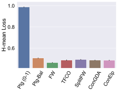
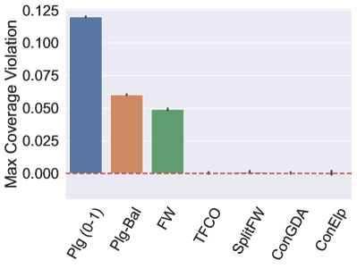
(c) CovType

Figure 13: Optimizing the H-mean loss subject to the coverage constraint $\max_{i}|\sum_{j}C_{ji}\,-\,\pi_{i}|\leq 0.01$. The plots on the left show the H-mean loss on the test set and those on the right show the coverage violation $\max_{i}|\sum_{j}C_{ji}\,-\,\pi_{i}|-0.01$ on the test set. Lower H-mean value are better, and the constraint values need to be $\leq 0$.

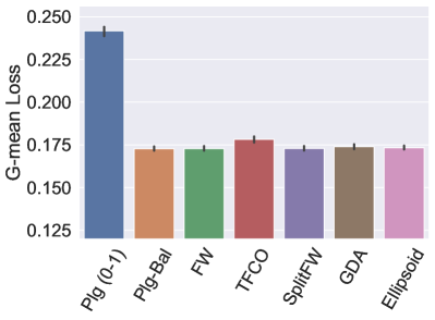
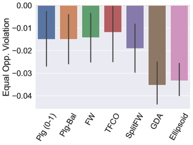
(a) Adult

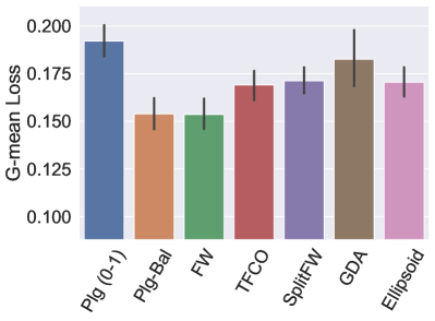
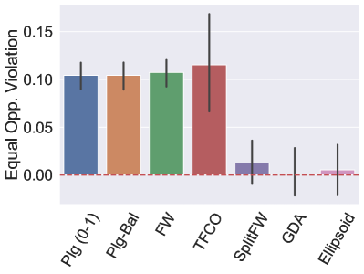
(b) Crimes

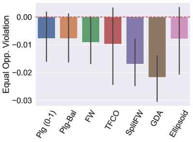
(c) Default

Figure 14: Optimizing the G-mean loss subject to the Equal Opportunity constraint $\leq 0.01$. The plots on the left show the G-mean loss on the test set and those on the right show the equal opportunity violation (needs to be $\leq 0$) on the test set. Lower G-mean values are better.

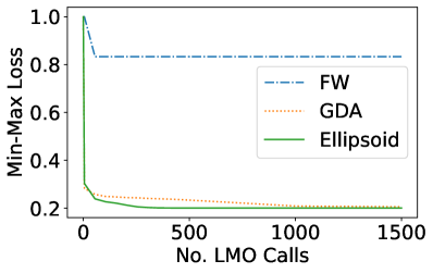
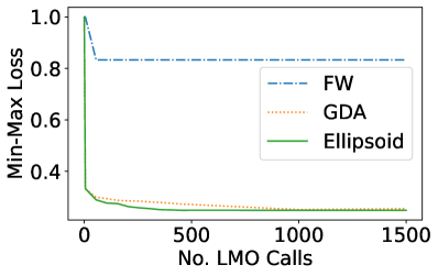
(a) SatImage

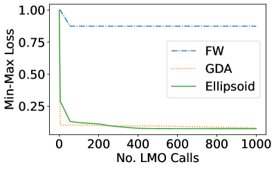
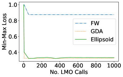
(b) MACHO

Figure 15: Optimizing the Min-max loss: Comparison of performance of the Frank-Wolfe, GDA and ellipsoid methods as a function of the number of LMO calls. The plot on the left is for train data and on the right is for test data. Lower values are better. Because the min-max loss is non-smooth, Frank-Wolfe is seen to converge to a sub-optimal classifier.

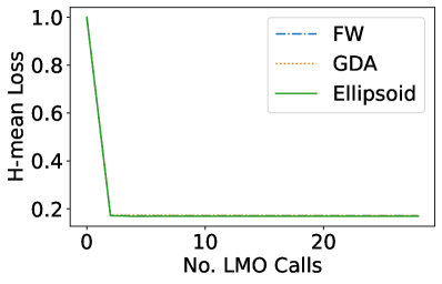
(a) SatImage

(b) MACHO

Figure 16: Optimizing the Hmean loss: Comparison of performance of the Frank-Wolfe, GDA and ellipsoid methods as a function of the number of LMO calls. The plot on the left is for Train data and on the right is for Test data. Lower values are better.

(a) Adult

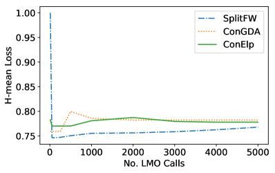
(b) Abalone

Figure 17: Optimizing the H-mean loss subject to the coverage constraint $\max_{i}|\sum_{j}C_{ji}\,-\,\pi_{i}|\leq 0.01$. The plots on the left show the H-mean loss on the train set and those on the right show the coverage violation $\max_{i}|\sum_{j}C_{ji}\,-\,\pi_{i}|-0.01$ on the train set. Lower H-mean value are better, and the constraint values need to be $\leq 0$.

Table 12: Comparison of the plug-in and weighted logistic regression (WLR) based LMOs on the task of optimizing the (convex) H-mean loss. The number of iterations, i.e. calls to the LMO, is fixed at 100. Lower values are better. The results are averaged over 10 random train-test splits

Dataset	FW		Ellipsoid		GDA
	Plugin	WLR	Plugin	WLR	Plugin	WLR
Aba	$0.812\pm 0.017$	$\textbf{0.798}\pm\textbf{0.013}$	$\textbf{0.815}\pm\textbf{0.017}$	$0.817\pm 0.012$	$0.841\pm 0.032$	$\textbf{0.837}\pm\textbf{0.035}$
PgB	$0.127\pm 0.039$	$\textbf{0.079}\pm\textbf{0.015}$	$0.111\pm 0.026$	$\textbf{0.079}\pm\textbf{0.018}$	$0.122\pm 0.032$	$\textbf{0.084}\pm\textbf{0.018}$
MAC	$\textbf{0.124}\pm\textbf{0.017}$	$0.245\pm 0.027$	$\textbf{0.125}\pm\textbf{0.017}$	$0.247\pm 0.027$	$\textbf{0.124}\pm\textbf{0.016}$	$0.206\pm 0.029$
Sat	$0.171\pm 0.007$	$\textbf{0.170}\pm\textbf{0.007}$	$0.170\pm 0.006$	$\textbf{0.167}\pm\textbf{0.006}$	$0.171\pm 0.007$	$\textbf{0.170}\pm\textbf{0.006}$
Cov	$0.466\pm 0.001$	$\textbf{0.450}\pm\textbf{0.001}$	$0.466\pm 0.001$	$\textbf{0.451}\pm\textbf{0.001}$	$0.463\pm 0.001$	$\textbf{0.447}\pm\textbf{0.001}$

Table 13: Performance metrics of a Random Classifiers on the Dataset. Lower Values are better.

Dataset	H-mean Loss	micro-F1
Communities & Crime	0.506	0.503
COMPAS	0.501	0.504
Law School	0.501	0.499
Default	0.499	0.498
Adult	0.499	0.499
Abalone	0.940	0.918
Pgblk	0.839	0.794
MACHO	0.914	0.874
SatImage	0.835	0.832
CovType	0.858	0.857

B.3 Additional Experimental Results

We report the H-mean Loss and micro-F measures of a random classifier on our datasets in Table 13. We also present additional results for the experiments described in Section 8: (i) Performance on Constrained Problems (Section 8.5): See Figures 13– 14. (ii) Practical Guidance on Algorithm Choice (Section 8.6): See Figures 15–17. (iii) Choice of LMO: Plug-in vs. Weighted Logistic Regression (Section 8.7): See Table 12.

References

• Abernethy and Wang (2017) J. D. Abernethy and J.-K. Wang. On Frank-Wolfe and equilibrium computation. In NIPS, 2017.
• Agarwal et al. (2018) A. Agarwal, A. Beygelzimer, M. Dudik, J. Langford, and H. Wallach. A reductions approach to fair classification. In ICML, 2018.
• Alabi et al. (2018) D. Alabi, N. Immorlica, and A. Kalai. Unleashing linear optimizers for group-fair learning and optimization. In COLT, 2018.
• Alcock et al. (2000) C. Alcock, R. A. Allsman, D. R. Alves, T. S. Axelrod, A. C. Becker, D. P. Bennett, K. H. Cook, N. Dalal, A. J. Drake, K. C. Freeman, et al. The MACHO project: Microlensing results from 5.7 years of large magellanic cloud observations. The Astrophysical Journal, 542(1):281, 2000.
• Angwin et al. (2016) J. Angwin, J. Larson, S. Mattu, and L. Kirchner. Machine bias. ProPublica, May, 23, 2016.
• Bartlett et al. (2006) P. L. Bartlett, M. I. Jordan, and J. D. McAuliffe. Convexity, classification, and risk bounds. Journal of the American Statistical Association, 101(473):138–156, 2006.
• Blumer et al. (1989) A. Blumer, A. Ehrenfeucht, D. Haussler, and M. Warmuth. Learnability and the Vapnik-Chervonenkis dimension. Journal of the ACM, 36:929–965, 1989.
• Boyd and Vandenberghe (2004) S. Boyd and L. Vandenberghe. Convex Optimization. Cambridge University Press, 2004.
• Bubeck (2015) S. Bubeck. Convex optimization: Algorithms and complexity. Foundations and Trends in Machine Learning, 8:231–358, 2015.
• Calauzènes et al. (2012) C. Calauzènes, N. Usunier, and P. Gallinari. On the (non-)existence of convex, calibrated surrogate losses for ranking. In NIPS, 2012.
• Celis et al. (2019) L. E. Celis, L. Huang, V. Keswani, and N. K. Vishnoi. Classification with fairness constraints: A meta-algorithm with provable guarantees. In FAT, 2019.
• Chen et al. (2017) R. Chen, B. Lucier, Y. Singer, and V. Syrgkanis. Robust optimization for non-convex objectives. arXiv preprint arXiv:1707.01047, 2017.
• Cormier et al. (2016) Q. Cormier, M.M. Fard, K. Canini, and M. Gupta. Launch and iterate: Reducing prediction churn. In NIPS, 2016.
• Cotter et al. (2019a) A. Cotter, H. Jiang, and K. Sridharan. Two-player games for efficient non-convex constrained optimization. In ALT, 2019a.
• Cotter et al. (2019b) A. Cotter, H. Jiang, S. Wang, T. Narayan, M. Gupta, S. You, and K. Sridharan. Optimization with non-differentiable constraints with applications to fairness, recall, churn, and other goals. Journal of Machine Learning Research, 2019b.
• Cotter et al. (2019) A. Cotter, H. Narasimhan, and M. Gupta. On making stochastic classifiers deterministic. In NeurIPS, 2019.
• Danskin (2012) J. M. Danskin. The theory of max-min and its application to weapons allocation problems, volume 5. Springer Science & Business Media, 2012.
• Dembczynski et al. (2011) K. Dembczynski, W. Waegeman, W. Cheng, and E. Hüllermeier. An exact algorithm for F-measure maximization. In NIPS, 2011.
• Dembczynski et al. (2013) K. Dembczynski, A. Jachnik, W. Kotlowski, W. Waegeman, and E. Hullermeier. Optimizing the F-measure in multi-label classification: Plug-in rule approach versus structured loss minimization. In ICML, 2013.
• Dembczyński et al. (2017) K. Dembczyński, W. Kotłowski, O. Koyejo, and N. Natarajan. Consistency analysis for binary classification revisited. In ICML, 2017.
• Donini et al. (2018) M. Donini, L. Oneto, S. Ben-David, J.S. Shawe-Taylor, and M. Pontil. Empirical risk minimization under fairness constraints. In NeurIPS, 2018.
• Duchi et al. (2010) J. Duchi, L. Mackey, and M. Jordan. On the consistency of ranking algorithms. In ICML, 2010.
• Eban et al. (2017) E. Eban, M. Schain, A. Mackey, A. Gordon, R. Rifkin, and G. Elidan. Scalable learning of non-decomposable objectives. In AISTATS, 2017.
• Elkan (2001) C. Elkan. The foundations of cost-sensitive learning. In IJCAI, 2001.
• Esuli and Sebastiani (2015) A. Esuli and F. Sebastiani. Optimizing text quantifiers for multivariate loss functions. ACM Transactions on Knowledge Discovery and Data, 9(4):Article 27, 2015.
• Finocchiaro et al. (2020) J. Finocchiaro, R. M. Frongillo, and B. Waggoner. Embedding dimension of polyhedral losses. In COLT, 2020.
• Frank and Asuncion (2010) A. Frank and A. Asuncion. UCI machine learning repository. URL: http://archive.ics.uci.edu/ml, 2010.
• Frank and Wolfe (1956) M. Frank and P. Wolfe. An algorithm for quadratic programming. Naval Research Logistics Quarterly, 3(1-2):95–110, 1956.
• Gao and Sebastiani (2015) W. Gao and F. Sebastiani. Tweet sentiment: From classification to quantification. In ASONAM, 2015.
• Gao and Zhou (2011) W. Gao and Z.-H. Zhou. On the consistency of multi-label learning. In COLT, 2011.
• Gidel et al. (2018) G. Gidel, F. Pedregosa, and S. Lacoste-Julien. Frank-wolfe splitting via augmented lagrangian method. In AISTATS, 2018.
• Goh et al. (2016) G. Goh, A. Cotter, M. Gupta, and M.P. Friedlander. Satisfying real-world goals with dataset constraints. In NIPS, 2016.
• Hardt et al. (2016) M. Hardt, E. Price, and N. Srebro. Equality of opportunity in supervised learning. In NIPS, 2016.
• Hiranandani et al. (2019) G. Hiranandani, S. Boodaghians, R. Mehta, and O. Koyejo. Multiclass performance metric elicitation. NeurIPS, 2019.
• Hiranandani et al. (2021) G. Hiranandani, J. Mathur, H. Narasimhan, M. M. Fard, and O. Koyejo. Optimizing black-box metrics with iterative example weighting. In ICML, 2021.
• Jaggi (2013) M. Jaggi. Revisiting Frank-Wolfe: Projection-free sparse convex optimization. In ICML, 2013.
• Joachims (2005) T. Joachims. A support vector method for multivariate performance measures. In ICML, 2005.
• Kar et al. (2014) P. Kar, H. Narasimhan, and P. Jain. Online and stochastic gradient methods for non-decomposable loss functions. In NeurIPS, 2014.
• Kar et al. (2016) P. Kar, S. Li, H. Narasimhan, S. Chawla, and F. Sebastiani. Online optimization methods for the quantification problem. In KDD, 2016.
• Kearns et al. (2018) M. Kearns, S. Neel, A. Roth, and Z.S. Wu. Preventing fairness gerrymandering: Auditing and learning for subgroup fairness. In ICML, 2018.
• Kennedy et al. (2009) K. Kennedy, B. M. Namee, and S. J. Delany. Learning without default: A study of one-class classification and the low-default portfolio problem. In ICAICS, 2009.
• Kim et al. (2011) D.-W. Kim, P. Protopapas, Y.-I. Byun, C. Alcock, R. Khardon, and M. Trichas. Quasi-stellar object selection algorithm using time variability and machine learning: Selection of 1620 quasi-stellar object candidates from macho large magellanic cloud database. The Astrophysical Journal, 735(2):68, 2011.
• Kim et al. (2013) J-D. Kim, Y. Wang, and Y. Yasunori. The genia event extraction shared task, 2013 edition - overview. ACL, 2013.
• Koyejo et al. (2014) O. Koyejo, N. Natarajan, P. Ravikumar, and I.S. Dhillon. Consistent binary classification with generalized performance metrics. In NIPS, 2014.
• Krizhevsky (2009) A. Krizhevsky. Learning multiple layers of features from tiny images. Technical report, University of Toronto, 2009.
• Kumar et al. (2021) A. Kumar, H. Narasimhan, and A. Cotter. Implicit rate-constrained optimization of non-decomposable objectives. In ICML, 2021.
• Lawrence et al. (1998) S. Lawrence, I. Burns, A. Back, A-C. Tsoi, and C.L. Giles. Neural network classification and prior class probabilities. In Neural Networks: Tricks of the Trade, LNCS, pages 1524:299–313. 1998.
• Lee et al. (2004) Y. Lee, Y. Lin, and G. Wahba. Multicategory support vector machines: Theory and application to the classification of microarray data. Journal of the American Statistical Association, 99(465):67–81, 2004.
• Lee et al. (2015) Y. T. Lee, A. Sidford, and S. C. Wong. A faster cutting plane method and its implications for combinatorial and convex optimization. In FOCS, 2015.
• Lewis (1991) D.D. Lewis. Evaluating text categorization. In Proceedings of the Workshop on Speech and Natural Language, HLT, 1991.
• Manning et al. (2008) C. D. Manning, P. Raghavan, and H. Schütze. Introduction to Information Retrieval. Cambridge University Press, 2008.
• Menon et al. (2013) A.K. Menon, H. Narasimhan, S. Agarwal, and S. Chawla. On the statistical consistency of algorithms for binary classification under class imbalance. In ICML, 2013.
• Narasimhan (2018) H. Narasimhan. Learning with complex loss functions and constraints. In AISTATS, 2018.
• Narasimhan et al. (2014) H. Narasimhan, R. Vaish, and S. Agarwal. On the statistical consistency of plug-in classifiers for non-decomposable performance measures. In NIPS, 2014.
• Narasimhan et al. (2015a) H. Narasimhan, P. Kar, and P. Jain. Optimizing non-decomposable performance measures: A tale of two classes. In ICML, 2015a.
• Narasimhan et al. (2015b) H. Narasimhan, H.G. Ramaswamy, A. Saha, and S. Agarwal. Consistent multiclass algorithms for complex performance measures. In ICML, 2015b.
• Narasimhan et al. (2020) H. Narasimhan, A. Cotter, Y. Zhou, S. Wang, and W. Guo. Approximate heavily-constrained learning with lagrange multiplier models. NeurIPS, 2020.
• Narasimhan et al. (2019) H. Narasimhan, A. Cotter, and M. Gupta. Optimizing generalized rate metrics with three players. In NeurIPS, 2019.
• Narici and Beckenstein (2010) L. Narici and E. Beckenstein. Topological Vector Spaces, Second Edition. Chapman & Hall/CRC Pure and Applied Mathematics. Taylor & Francis, 2010.
• Natarajan et al. (2016) N. Natarajan, O. Koyejo, P. Ravikumar, and I. Dhillon. Optimal classification with multivariate losses. In ICML, 2016.
• Nowak-Vila et al. (2020) A. Nowak-Vila, F. Bach, and A. Rudi. Consistent structured prediction with max-min margin markov networks. In ICML, 2020.
• Pan et al. (2016) W. Pan, H. Narasimhan, P. Kar, P. Protopapas, and H. G. Ramaswamy. Optimizing the multiclass F-measure via biconcave programming. In ICDM, 2016.
• Parambath et al. (2014) S.A.P. Parambath, N. Usunier, and Y. Grandvalet. Optimizing F-measures by cost-sensitive classification. In NIPS, 2014.
• Patrini et al. (2017) G. Patrini, A. Rozza, A. K. Menon, R. Nock, and L. Qu. Making deep neural networks robust to label noise: A loss correction approach. In CVPR, 2017.
• Pires et al. (2013) B. Á. Pires, C. Szepesvari, and M. Ghavamzadeh. Cost-sensitive multiclass classification risk bounds. In ICML, 2013.
• Ramaswamy et al. (2015) H. Ramaswamy, A. Tewari, and S. Agarwal. Convex calibrated surrogates for hierarchical classification. In ICML, 2015.
• Ramaswamy and Agarwal (2012) H. G. Ramaswamy and S. Agarwal. Classification calibration dimension for general multiclass losses. In NIPS, 2012.
• Ramaswamy et al. (2013) H. G. Ramaswamy, S. Agarwal, and A. Tewari. Convex calibrated surrogates for low-rank loss matrices with applications to subset ranking losses. In NIPS, 2013.
• Ramaswamy et al. (2018) H. G. Ramaswamy, A. Tewari, and S. Agarwal. Consistent algorithms for multiclass classification with an abstain option. Electronic Journal of Statistics, 12(1):530–554, 2018.
• Ravikumar et al. (2011) P. Ravikumar, A. Tewari, and E. Yang. On NDCG consistency of listwise ranking methods. In AISTATS, 2011.
• Sanyal et al. (2018) A. Sanyal, P. Kumar, P. Kar, S. Chawla, and F. Sebastiani. Optimizing non-decomposable measures with deep networks. Machine Learning, 107(8-10):1597–1620, 2018.
• Shalev-Shwartz (2011) S. Shalev-Shwartz. Online learning and online convex optimization. Foundations and trends in Machine Learning, 4(2):107–194, 2011.
• Steinitz (1913) E. Steinitz. Bedingt konvergente reihen und konvexe systeme. 1913.
• Steinwart (2007) I. Steinwart. How to compare different loss functions and their risks. Constructive Approximation, 26:225–287, 2007.
• Sun et al. (2006) Y. Sun, M.S. Kamel, and Y. Wang. Boosting for learning multiple classes with imbalanced class distribution. In ICDM, 2006.
• Tavker et al. (2020) S. K. Tavker, H. G. Ramaswamy, and H. Narasimhan. Consistent plug-in classifiers for complex objectives and constraints. In NeurIPS, 2020.
• Tewari and Bartlett (2007) A. Tewari and P. L. Bartlett. On the consistency of multiclass classification methods. Journal of Machine Learning Research, 8:1007–1025, 2007.
• Ting (2002) K. M. Ting. An instance-weighting method to induce cost-sensitive trees. IEEE Transactions on Knowledge and Data Engineering, 14(3):659–665, 2002.
• Vernet et al. (2011) E. Vernet, R. C. Williamson, and M. D. Reid. Composite multiclass losses. In NIPS, 2011.
• Vincent (1994) P. H. Vincent. An Introduction to Signal Detection and Estimation. Springer-Verlag, 1994.
• Wang and Yao (2012) S. Wang and X. Yao. Multiclass imbalance problems: Analysis and potential solutions. IEEE Transactions on Systems, Man, and Cybernetics, Part B: Cybernetics, 42(4):1119–1130, 2012.
• Wang et al. (2019) X. Wang, R. Li, B. Yan, and O. Koyejo. Consistent classification with generalized metrics. arXiv preprint arXiv:1908.09057, 2019.
• Wightman (1998) L. Wightman. Lsac national longitudinal bar passage study. Law School Admission Council, 1998.
• Yang and Koyejo (2020) F. Yang and O. Koyejo. On the consistency of top-k surrogate losses. In ICML, 2020.
• Yang et al. (2020) F. Yang, M. Cisse, and O. Koyejo. Fairness with overlapping groups; a probabilistic perspective. NeurIPS, 2020.
• Ye et al. (2012) N. Ye, K. M. A. Chai, W. S. Lee, and H. L. Chieu. Optimizing F-measures: A tale of two approaches. In ICML, 2012.
• Yuan and Wegkamp (2010) M. Yuan and M. Wegkamp. Classification methods with reject option based on convex risk minimization. Journal of Machine Learning Research, 11:111–130, 2010.
• Zafar et al. (2017a) M. B. Zafar, I. Valera, M. G. Rodriguez, and K. P. Gummadi. Fairness constraints: Mechanisms for fair classification. In AISTATS, 2017a.
• Zafar et al. (2017b) M. B. Zafar, I. Valera, M. G. Rodriguez, and K. P. Gummadi. Fairness beyond disparate treatment & disparate impact: Learning classification without disparate mistreatment. In WWW, 2017b.
• Zhang et al. (2020) M. Zhang, H. G. Ramaswamy, and S. Agarwal. Convex calibrated surrogates for the multi-label f-measure. In ICML, 2020.
• Zhang (2004a) T. Zhang. Statistical behavior and consistency of classification methods based on convex risk minimization. Annals of Statistics, 32(1):56–134, 2004a.
• Zhang (2004b) T. Zhang. Statistical analysis of some multi-category large margin classification methods. Journal of Machine Learning Research, 5:1225–1251, 2004b.
• Zinkevich (2003) M. Zinkevich. Online convex programming and generalized infinitesimal gradient ascent. In ICML, 2003.