Integrable delay-difference and delay-differential analogues of the KdV, Boussinesq, and KP equations

Abstract

Delay-difference and delay-differential analogues of the KdV and Boussinesq (BSQ) equations are presented. Each of them has the $N$-soliton solution and reduces to an already known soliton equation as the delay parameter approaches 0. In addition, a delay-differential analogue of the KP equation is proposed. We discuss its $N$-soliton solution and the limit as the delay parameter approaches 0. Finally, the relationship between the delay-differential analogues of the KdV, BSQ, and KP equations is clarified. Namely, reductions of the delay KP equation yield the delay KdV and delay BSQ equations.

Keywords:  delay-differential equations, delay-difference equations, the KdV equation, the Boussinesq equation, the KP equation, $N$-soliton solutions

1 Introduction

Delay-differential equations can often model and analyze systems involving feedback effects, such as infectious disease and traffic flow. In the stream of such studies, exact solutions of delay-differential equations have been obtained and discussed [1, 2, 3].

In recent years, research on integrable delay-differential equations is actively developing. For examples of ordinary differential equations, integrable delay-differential analogues of Painlevé equations have been introduced by several methods. Quispel et al. [4] considered a similarity reduction of the Lotka-Volterra (LV) equation, then obtained a delay-differential analogue of the first Painlevé equation. Ramani et al. [5, 6] considered the integrability test for delay-differential systems, then Grammaticos et al. [7] used it and obtained delay-differential analogues of some Painlevé equations. After these discoveries, various properties of the delay Painlevé equations were revealed from some viewpoints [8, 9, 10, 11, 12, 13, 14, 15].

On the other hand, exact solutions of integrable partial delay-differential equations have been studied. For example, a delay-differential analogue of the two-dimensional Toda lattice equation (2DTL) was addressed [16, 17]. To our knowledge, this is the first example of a delay soliton equation, which means a delay-differential equation with the $N$-soliton solution. Subsequently, in our previous study [18], we proposed a systematic method for constructing delay-difference and delay-differential analogues of soliton equations. As examples of this method, we constructed delay-difference and delay-differential analogues of the LV, Toda lattice (TL), and sine-Gordon (sG) equations with their $N$-soliton solutions. However, these delay soliton equations are just simple examples, and this method cannot be easily applied to some soliton equations including the KdV equation (this meaning is explained in Remark 2.7). Thus this method is not yet sufficient to discuss integrable properties of delay soliton equations, such as relationships to delay Painlevé equations.

In section 2 of this paper, we first propose integrable delay-difference and delay-differential analogues of the KdV equation and their $N$-soliton solutions by using the above method [18]. In detail, it is carried out by applying reduction and continuum limits to the discrete KP equation [19, 20]. As the delay parameter approaches $0$, this delay-differential analogues of the KdV equation (the delay KdV equation) reduces to the well-known KdV equation, and the same is true for the $N$-soliton solution. We can also obtain a delay Boussinesq (BSQ) equation by applying a transformation to the delay KdV equation. In section 3, we propose a delay-differential analogue of the KP equation by a transformation from the 2DTL. The Casorati determinant solution of this delay KP equation is obtained by using equivalence to the 2DTL. Similar to the KdV and BSQ cases, the delay KP equation and its $N$-soliton solution reduce to the KP equation and its $N$-soliton solution as the delay parameter approaches 0. Finally, we derive the above delay KdV and delay BSQ equations again by reductions of the delay KP equation.

2 An integrable delay KdV equation

In this section, we construct a delay-difference and delay-differential analogue of the KdV equation by using the method for constructing delay soliton equations [18]. An overview of this method is given as follows.

• We consider a reduction of the discrete KP equation. The reduction condition needs to include a free parameter $\alpha$ (such as (6)). Applying this reduction to the discrete KP equation, we obtain a discrete equation that depends on $\alpha$ (such as (7)). This discrete equation turns out to be a delay-difference analogue of a soliton equation.

• We apply a continuum limit to the above delay-difference soliton equation. In this continuum limit, the lattice parameter approaches $0$, and the parameter $\alpha$ approaches infinity (such as (14)). Then we obtain a delay-differential equation (such as (2.2)), which is considered as a delay-differential analogue of a soliton equation.

Following the above process, we first construct the delay discrete KdV equation by a reduction of the discrete KP equation (subsection 2.1). Then we obtain the delay semi-discrete KdV equation by continuum limit (subsection 2.2). Finally we obtain the delay KdV equation by continuum limit (subsection 2.3).

2.1 The delay discrete KdV equation

We start from the discrete KP equation [19, 20]

$$a(b-c)f_{n+1,m,k}f_{n,m+1,k+1}+b(c-a)f_{n,m+1,k}f_{n+1,m,k+1}$$

$$\hskip 56.9055pt+c(a-b)f_{n,m,k+1}f_{n+1,m+1,k}=0$$ (1)

and its $N$-soliton solution in the Gram determinant form [21]

$$f_{n,m,k}=\det\left(\delta_{ij}+\frac{\phi_{i}\psi_{j}}{p_{i}-q_{j}}\right)_{1\leq i,j\leq N}=\det\left(\delta_{ij}+\frac{\phi_{j}\psi_{j}}{p_{i}-q_{j}}\right)_{1\leq i,j\leq N}\,,$$ (2)

$$\phi_{i}(n,m,k)=\beta_{i}^{-1}(1-ap_{i})^{-n}(1-bp_{i})^{-m}(1-cp_{i})^{-k}\,,$$

$$\psi_{i}(n,m,k)=\gamma_{i}(1-aq_{i})^{n}(1-bq_{i})^{m}(1-cq_{i})^{k}\,,$$

where $a,b,c,p_{i},q_{i},\beta_{i},\gamma_{i}$ are real constants. Using the function

$$\Phi_{i}(n,m,k)=\frac{\gamma_{i}}{\beta_{i}}\left(\frac{1-aq_{i}}{1-ap_{i}}\right)^{n}\left(\frac{1-bq_{i}}{1-bp_{i}}\right)^{m}\left(\frac{1-cq_{i}}{1-cp_{i}}\right)^{k}\,,$$

we can describe solution (2) as

$$f_{n,m,k}=\det\left(\delta_{ij}+\frac{\Phi_{j}}{p_{i}-q_{j}}\right)_{1\leq i,j\leq N}\,.$$

If we ignore the constant doubling of $\beta_{i}$ and $\gamma_{i}$, this solution can be rewritten as follows:

$$f_{n,m,k}=\det\left(\delta_{ij}+\frac{\Phi_{j}}{p_{i}-q_{j}}\right)_{1\leq i,j\leq N}=\sum_{I\subset\{1,\ldots,N\}}\prod_{i\in I}\Phi_{i}\prod_{i<j,\ i,j\in I}\frac{(p_{i}-p_{j})(q_{i}-q_{j})}{(p_{i}-q_{j})(q_{i}-p_{j})}\,.$$ (3)

For convenience, we apply the transformation $n^{\prime}=2(n+m),\ \ m^{\prime}=2(n-m)$ to the discrete KP equation (2.1) and its solution (3), then rewrite $n^{\prime},m^{\prime}$ by $n,m$ again. Through the transformation, equation (2.1) is transformed into

$$a(b-c)f_{n+2,m+2,k}f_{n+2,m-2,k+1}+b(c-a)f_{n+2,m-2,k}f_{n+2,m+2,k+1}$$

$$\hskip 56.9055pt+c(a-b)f_{n,m,k+1}f_{n+4,m,k}=0\,.$$ (4)

Replacing $p_{i}$ and $q_{i}$ by $p_{i}/a$ and $q_{i}/a$ respectively, and setting $\mu_{i}=\gamma_{i}/\beta_{i}$, solution (3) is transformed into

$$f_{n,m,k}=\det\left(\delta_{ij}+\frac{\Phi_{j}}{p_{i}-q_{j}}\right)_{1\leq i,j\leq N}=\sum_{I\subset\{1,\ldots,N\}}\prod_{i\in I}\Phi_{i}\prod_{i<j,\ i,j\in I}\frac{(p_{i}-p_{j})(q_{i}-q_{j})}{(p_{i}-q_{j})(q_{i}-p_{j})}\,,$$ (5)

$$\Phi_{i}=\mu_{i}\left(\frac{1-q_{i}}{1-p_{i}}\frac{a-bq_{i}}{a-bp_{i}}\right)^{n/4}\left(\frac{1-q_{i}}{1-p_{i}}\frac{a-bp_{i}}{a-bq_{i}}\right)^{m/4}\left(\frac{a-cq_{i}}{a-cp_{i}}\right)^{k}\,.$$

Now, we apply the reduction condition

$$f_{n,m,k+1}=f_{n-2-2\nu,m-2-2\alpha,k}$$ (6)

to the transformed discrete KP equation (2.1) and its solution (5), where the parameters $\alpha$ and $\nu$ are fixed values considered as the delays. Setting $c=-a$ and $\epsilon\delta=(b-a)/(b+a)$, the transformed discrete KP equation (2.1) reduces to the following bilinear equation

$$\epsilon\delta f_{n+3+\nu}^{m+1+\alpha}f_{n-3-\nu}^{m-1-\alpha}+f_{n+1+\nu}^{m+3+\alpha}f_{n-1-\nu}^{m-3-\alpha}-(1+\epsilon\delta)f_{n+1+\nu}^{m-1+\alpha}f_{n-1-\nu}^{m+1-\alpha}=0\,,$$ (7)

where $f_{n}^{m}\equiv f_{n,m,k}$ (the dependence of $k$ is omitted). The variables $n$ and $m$ are considered to be the discrete space and time variables respectively. We can rewrite the bilinear equation (7) as follows by using Hirota’s D-operators:

$$(2\sinh\left(D_{n}+D_{m}+\nu D_{n}+\alpha D_{m}\right)\sinh(2D_{m})$$

$$\hskip 56.9055pt+2\epsilon\delta\sinh(D_{n}+D_{m})\sinh\left(2D_{n}+\nu D_{n}+\alpha D_{m}\right))f_{n}^{m}\cdot f_{n}^{m}=0\,.$$ (8)

Here Hirota’s D-operators are defined by

$$D^{l}_{t}{g(t)}\cdot{h(t)}=\left(\frac{\partial}{\partial t}-\frac{\partial}{\partial s}\right)^{l}g(t)h(s)\Bigr{|}_{s=t}\,,\qquad e^{rD_{m}}g_{m}\cdot h_{m}=g_{m+r}h_{m-r}\,.$$

We can consider equation (7) (or (2.1)) is the bilinear form of the delay-difference analogue of the KdV equation. By putting $\nu=\alpha=0$ and $\epsilon=1$, we obtain the bilinear form of the discrete KdV equation, which is called the difference-difference KdV equation [22, 23]. We call equation (7) the bilinear form of the delay discrete KdV equation.

Next we consider the reduction of the $N$-soliton solution. To realize the reduction condition (6), it is sufficient to impose the constraint

$$1=\left(\frac{1-q_{i}}{1-p_{i}}\frac{a-bq_{i}}{a-bp_{i}}\right)^{(1+\nu)/2}\left(\frac{1-q_{i}}{1-p_{i}}\frac{a-bp_{i}}{a-bq_{i}}\right)^{(1+\alpha)/2}\left(\frac{a-cq_{i}}{a-cp_{i}}\right)$$

on the $N$-soliton solution (5). The reason is as follows. By this constraint, we can obtain the relation

$$\Phi_{i}(n,m,k+1)$$

$$= \mu_{i}\left(\frac{1-q_{i}}{1-p_{i}}\frac{a-bq_{i}}{a-bp_{i}}\right)^{n/4}\left(\frac{1-q_{i}}{1-p_{i}}\frac{a-bp_{i}}{a-bq_{i}}\right)^{m/4}\left(\frac{a-cq_{i}}{a-cp_{i}}\right)^{k+1}$$

$$= \mu_{i}\left(\frac{1-q_{i}}{1-p_{i}}\frac{a-bq_{i}}{a-bp_{i}}\right)^{(n-2-2\nu)/4}\left(\frac{1-q_{i}}{1-p_{i}}\frac{a-bp_{i}}{a-bq_{i}}\right)^{(m-2-2\alpha)/4}\left(\frac{a-cq_{i}}{a-cp_{i}}\right)^{k}$$

$$= \Phi_{i}(n-2-2\nu,m-2-2\alpha,k)\,.$$

Solution (5) with this relation $\Phi_{i}(n,m,k+1)=\Phi_{i}(n-2-2\nu,m-2-2\alpha,k)$ satisfies the condition (6): $f_{n,m,k+1}=f_{n-2-2\nu,m-2-2\alpha,k}$, because $f$ is a function of $\Phi_{i}(n,m,k)\ (1\leq i\leq N)$. Now, using $c=-a$, $\epsilon\delta=(b-a)/(b+a)$ and setting $k=0$, we obtain the $N$-soliton solution of the delay discrete KdV equation (7) as follows:

$$f_{n}^{m}=\det\left(\delta_{ij}+\frac{\Phi_{j}}{p_{i}-q_{j}}\right)_{1\leq i,j\leq N}=\sum_{I\subset\{1,\ldots,N\}}\prod_{i\in I}\Phi_{i}\prod_{i<j,\ i,j\in I}\frac{(p_{i}-p_{j})(q_{i}-q_{j})}{(p_{i}-q_{j})(q_{i}-p_{j})}\,,$$ (9)

$$\Phi_{i}=\mu_{i}\left(\frac{1-q_{i}}{1-p_{i}}\frac{1-q_{i}-\epsilon\delta(1+q_{i})}{1-p_{i}-\epsilon\delta(1+p_{i})}\right)^{n/4}\left(\frac{1-q_{i}}{1-p_{i}}\frac{1-p_{i}-\epsilon\delta(1+p_{i})}{1-q_{i}-\epsilon\delta(1+q_{i})}\right)^{m/4}\,,$$

$$1=\left(\frac{1-q_{i}}{1-p_{i}}\frac{1-q_{i}-\epsilon\delta(1+q_{i})}{1-p_{i}-\epsilon\delta(1+p_{i})}\right)^{(1+\nu)/2}\left(\frac{1-q_{i}}{1-p_{i}}\frac{1-p_{i}-\epsilon\delta(1+p_{i})}{1-q_{i}-\epsilon\delta(1+q_{i})}\right)^{(1+\alpha)/2}\left(\frac{1+q_{i}}{1+p_{i}}\right)\,.$$

The solution (9) in the case of $\nu=\alpha=0$ and $\epsilon=1$ is equivalent to the $N$-soliton solution of the discrete KdV equation [22].

Now, let us derive the nonlinear form of the delay discrete KdV equation. We consider the dependent variable transformation

$$w_{n}^{m}=\frac{f_{n+2+(\nu/2)}^{m+(\alpha/2)}f_{n-2-(\nu/2)}^{m-(\alpha/2)}}{f_{n+(\nu/2)}^{m+2+(\alpha/2)}f_{n-(\nu/2)}^{m-2-(\alpha/2)}}\,.$$ (10)

Through this transformation, the bilinear equation (7) is transformed into

$$\frac{w_{n+1+\nu}^{m-1+\alpha}w_{n-1-\nu}^{m+1-\alpha}}{w_{n+1+\nu}^{m+3+\alpha}w_{n-1-\nu}^{m-3-\alpha}}=\frac{\left(1+\epsilon\delta w_{n+3+\nu}^{m+1+\alpha}w_{n+1}^{m-1}\right)\left(1+\epsilon\delta w_{n-1}^{m+1}w_{n-3-\nu}^{m-1-\alpha}\right)}{\left(1+\epsilon\delta w_{n+1+\nu}^{m+3+\alpha}w_{n-1}^{m+1}\right)\left(1+\epsilon\delta w_{n+1}^{m-1}w_{n-1-\nu}^{m-3-\alpha}\right)}\,.$$ (11)

This is the nonlinear form of the delay discrete KdV equation. When $\alpha=\nu=0$ and $\epsilon=1$, (11) is the division of the following two equations:

$$\frac{w_{n+1}^{m-1}}{w_{n+1}^{m+3}}=\frac{1+\delta w_{n+3}^{m+1}w_{n+1}^{m-1}}{1+\delta w_{n+1}^{m+3}w_{n-1}^{m+1}}\,,$$ (12)

$$\frac{w_{n-1}^{m-3}}{w_{n-1}^{m+1}}=\frac{1+\delta w_{n+1}^{m-1}w_{n-1}^{m-3}}{1+\delta w_{n-1}^{m+1}w_{n-3}^{m-1}}\,.$$ (13)

Both (12) and (13) are equivalent to the discrete KdV equation [22]

$$\frac{1}{w_{n}^{m+2}}-\frac{1}{w_{n}^{m-2}}=\delta(w_{n+2}^{m}-w_{n-2}^{m})\,.$$

Remark 2.1.

Transformation (10) is obtained by an analogy to the case of the discrete KdV equation.

First, let us remind of the case of the discrete KdV equation. The bilinear form is

$$\delta f_{n+3}^{m+1}f_{n-3}^{m-1}+f_{n+1}^{m+3}f_{n-1}^{m-3}-(1+\delta)f_{n+1}^{m-1}f_{n-1}^{m+1}=0\,,$$

which is rewritten as

$$(1+\delta)\frac{f_{n+1}^{m-1}f_{n-1}^{m+1}}{f_{n+1+\nu}^{m+3}f_{n-1}^{m-3}}=1+\delta\frac{f_{n+3}^{m+1}f_{n-3}^{m-1}}{f_{n+1+\nu}^{m+3}f_{n-1}^{m-3}}\,.$$

Putting $w_{n}^{m}=(f_{n+2}^{m}f_{n-2}^{m})/(f_{n}^{m+2}f_{n}^{m-2})$, we obtain

$$(1+\delta)\frac{f_{n+1}^{m-1}f_{n-1}^{m+1}}{f_{n+1+\nu}^{m+3}f_{n-1}^{m-3}}=1+\delta w_{n+1}^{m+1}w_{n-1}^{m-1}\,.$$

By shifting and combining this equation, we obtain the nonlinear form (12) (or (13)).

Now, inspired by this derivation, we rewrite delayed bilinear equation (7) as

$$(1+\epsilon\delta)\frac{f_{n+1+\nu}^{m-1+\alpha}f_{n-1-\nu}^{m+1-\alpha}}{f_{n+1+\nu}^{m+3+\alpha}f_{n-1-\nu}^{m-3-\alpha}}=1+\epsilon\delta\frac{f_{n+3+\nu}^{m+1+\alpha}f_{n-3-\nu}^{m-1-\alpha}}{f_{n+1+\nu}^{m+3+\alpha}f_{n-1-\nu}^{m-3-\alpha}}\,.$$

Putting $w_{n}^{m}$ as (10), we obtain

$$(1+\epsilon\delta)\frac{f_{n+1+\nu}^{m-1+\alpha}f_{n-1-\nu}^{m+1-\alpha}}{f_{n+1+\nu}^{m+3+\alpha}f_{n-1-\nu}^{m-3-\alpha}}=1+\epsilon\delta w_{n+1+(\nu/2)}^{m+1+(\alpha/2)}w_{n-1-(\nu/2)}^{m-1-(\alpha/2)}\,.$$

By shifting and combining this equation, we obtain the nonlinear form (11).

Remark 2.2.

Let us describe the delay discrete KdV equation (11) in other independent variables. We apply the transformation

$$n^{\prime}=\frac{1}{4}(n+m),\qquad m^{\prime}=\frac{1}{4}(-n+m),\qquad\nu^{\prime}=\frac{1}{4}(\nu+\alpha),\qquad\alpha^{\prime}=\frac{1}{4}(-\nu+\alpha)$$

to equation (11), then rewrite $n^{\prime},m^{\prime},\alpha^{\prime},\nu^{\prime}$ by $n,m,\alpha,\nu$ again. Through this transformation, equation (11) is transformed into

$$\frac{w_{n+\nu}^{m+\alpha}w_{n-\nu}^{m+1-\alpha}}{w_{n+1+\nu}^{m+1+\alpha}w_{n-1-\nu}^{m-\alpha}}=\frac{\left(1+\delta w_{n+1+\nu}^{m+\alpha}w_{n}^{m}\right)\left(1+\delta w_{n}^{m+1}w_{n-1-\nu}^{m+1-\alpha}\right)}{\left(1+\delta w_{n+1+\nu}^{m+1+\alpha}w_{n}^{m+1}\right)\left(1+\delta w_{n}^{m}w_{n-1-\nu}^{m-\alpha}\right)}\,.$$

When $\alpha=\nu=0$, this equation is the division of the following two equations:

$$\frac{w_{n+1}^{m+1}}{w_{n}^{m}}=\frac{1+\delta w_{n+1}^{m+1}w_{n}^{m+1}}{1+\delta w_{n+1}^{m}w_{n}^{m}}\,,\qquad\frac{w_{n}^{m+1}}{w_{n-1}^{m}}=\frac{1+\delta w_{n}^{m+1}w_{n-1}^{m+1}}{1+\delta w_{n}^{m}w_{n-1}^{m}}\,,$$

which are equivalent to the discrete KdV equation

$$\frac{1}{w_{n+1}^{m+1}}-\frac{1}{w_{n}^{m}}=\delta(w_{n+1}^{m}-w_{n}^{m+1})\,.$$

2.2 The delay semi-discrete KdV equation

We propose the following continuum limit to the delay discrete KdV equation (7) and its $N$-soliton solution (9):

$$\delta\to 0\,,\qquad\frac{m\delta}{4}=t\,,\qquad\frac{\alpha\delta}{4}=\tau=\mathrm{const}.\,,$$ (14)

where $t$ is the continuous time variable, and $\tau$ is a fixed value considered as the time-delay. Applying the continuum limit (14) to (7) and (9), we obtain the bilinear equation

$$D_{t}{f_{n+1+\nu}(t+\tau)}\cdot{f_{n-1-\nu}(t-\tau)}+\epsilon f_{n+3+\nu}(t+\tau)f_{n-3-\nu}(t-\tau)$$

$$\hskip 56.9055pt-\epsilon f_{n+1+\nu}(t+\tau)f_{n-1-\nu}(t-\tau)=0$$ (15)

and its $N$-soliton solution

$$f_{n}(t)=\det\left(\delta_{ij}+\frac{\Phi_{j}}{p_{i}-q_{j}}\right)_{1\leq i,j\leq N}=\sum_{I\subset\{1,\ldots,N\}}\prod_{i\in I}\Phi_{i}\prod_{i<j,\ i,j\in I}\frac{(p_{i}-p_{j})(q_{i}-q_{j})}{(p_{i}-q_{j})(q_{i}-p_{j})}\,,$$ (16)

$$\Phi_{i}=\mu_{i}\left(\frac{1-q_{i}}{1-p_{i}}\right)^{n/2}\exp\left\{\epsilon\left(-\frac{1+p_{i}}{1-p_{i}}+\frac{1+q_{i}}{1-q_{i}}\right)t\right\}\,,$$

$$1=\left(\frac{1-q_{i}}{1-p_{i}}\right)^{1+\nu}\exp\left\{2\tau\epsilon\left(-\frac{1+p_{i}}{1-p_{i}}+\frac{1+q_{i}}{1-q_{i}}\right)\right\}\left(\frac{1+q_{i}}{1+p_{i}}\right)\,.$$

Bilinear equation (2.2) is rewritten as

$$\left(\sinh\left(D_{n}+\nu D_{n}+\tau D_{t}\right)D_{t}+2\epsilon\sinh(D_{n})\sinh\left(2D_{n}+\nu D_{n}+\tau D_{t}\right)\right)f_{n}(t)\cdot f_{n}(t)$$

$$\hskip 56.9055pt=0\,.$$ (17)

We can claim equation (2.2) (or (2.2)) is the bilinear form of the delay semi-discrete KdV equation. By putting $\nu=\tau=0$ and $\epsilon=1$, we can obtain the bilinear form of the semi-discrete KdV equation, which is called the differential-difference KdV equation [22]. In addition, the solution (16) in the case of $\nu=\tau=0$ and $\epsilon=1$ is equivalent to the $N$-soliton solution of the semi-discrete KdV equation [22].

Remark 2.3.

The delay LV equation [18] is given by

$$D_{t}{f_{n}(t+\tau)}\cdot{f_{n-1}(t-\tau)}-f_{n+1}(t+\tau)f_{n-2}(t-\tau)+f_{n}(t+\tau)f_{n-1}(t-\tau)=0\,.$$

This equation can be derived by applying the transformation

$$n\rightarrow 2n\,,\quad t\rightarrow-t\,,\quad\tau\rightarrow-\tau\,,\quad\nu=0\,,\quad\epsilon=1$$

to the delay semi-discrete KdV equation (2.2).

Remark 2.4.

The semi-discrete KP equation [24] is given by

$$D_{t}f_{n+2}^{k}(t)\cdot f_{n}^{k+1}(t)+\epsilon(f_{n+2}^{k}(t)f_{n}^{k+1}(t)-f_{n+2}^{k+1}(t)f_{n}^{k}(t))=0\,.$$

Applying the reduction condition $f_{n}^{k+1}(t)=f_{n+4+2\nu}^{k}(t+2\tau)$ to this equation, we can derive the delay semi-discrete KdV equation (2.2).

Now, let us derive the nonlinear form of the delay semi-discrete KdV equation. We consider the dependent variable transformation

$$w_{n}(t)=\frac{f_{n+2+(\nu/2)}(t+\tau/2)f_{n-2-(\nu/2)}(t-\tau/2)}{f_{n+(\nu/2)}(t+\tau/2)f_{n-(\nu/2)}(t-\tau/2)}\,.$$ (18)

Through this transformation, the bilinear equation (2.2) is transformed into

$$\frac{\mathrm{d}}{\mathrm{d}t}\log\frac{w_{n+1+\nu}(t+\tau)}{w_{n-1-\nu}(t-\tau)} =-\epsilon w_{n+3+\nu}(t+\tau)\ w_{n+1}(t)-\epsilon w_{n-1}(t)\ w_{n-3-\nu}(t-\tau)$$

$$\quad+\epsilon w_{n+1+\nu}(t+\tau)\ w_{n-1}(t)+\epsilon w_{n+1}(t)\ w_{n-1-\nu}(t-\tau)\,.$$ (19)

This is the nonlinear form of the delay semi-discrete KdV equation. When $\tau=\nu=0$ and $\epsilon=1$, (2.2) is the subtraction of the following two equations:

$$\frac{\mathrm{d}}{\mathrm{d}t}\log(w_{n+1}(t))=w_{n+1}(t)(w_{n-1}(t)-w_{n+3}(t))\,,$$ (20)

$$\frac{\mathrm{d}}{\mathrm{d}t}\log(w_{n-1}(t))=w_{n-1}(t)(w_{n-3}(t)-w_{n+1}(t))\,.$$ (21)

Both (20) and (21) are equivalent to the semi-discrete KdV equation [22]

$$\frac{\mathrm{d}}{\mathrm{d}t}\frac{1}{w_{n}(t)}=w_{n+2}(t)-w_{n-2}(t)\,.$$

Remark 2.5.

Similar to Remark 2.1, transformation (18) is obtained by an analogy to the case of the semi-discrete KdV equation.

First, let us remind of the case of the semi-discrete KdV equation. The bilinear form is

$$D_{t}{f_{n+1}(t)}\cdot{f_{n-1}(t)}+f_{n+3}(t)f_{n-3}(t)-f_{n+1}(t)f_{n-1}(t)=0\,,$$

which is rewritten as

$$\frac{\mathrm{d}}{\mathrm{d}t}\log\frac{f_{n+1}(t)}{f_{n-1}(t)}=1-\frac{f_{n+3}(t)f_{n-3}(t)}{f_{n+1}(t)f_{n-1}(t)}\,.$$

Putting $w_{n}(t)=(f_{n+2}(t)f_{n-2}(t))/(f_{n}(t)f_{n}(t))$, we obtain

$$\frac{\mathrm{d}}{\mathrm{d}t}\log\frac{f_{n+1}(t)}{f_{n-1}(t)}=1-w_{n+1}(t)w_{n-1}(t)\,.$$

By shifting and combining this equation, we obtain the nonlinear form (20) (or (21)).

Now, inspired by this derivation, we rewrite delayed bilinear equation (2.2) as

$$\frac{\mathrm{d}}{\mathrm{d}t}\log\frac{f_{n+1+\nu}(t+\tau)}{f_{n-1-\nu}(t-\tau)}=\epsilon-\epsilon\frac{f_{n+3+\nu}(t+\tau)f_{n-3-\nu}(t-\tau)}{f_{n+1+\nu}(t+\tau)f_{n-1-\nu}(t-\tau)}\,.$$

Putting $w_{n}(t)$ as (18), we obtain

$$\frac{\mathrm{d}}{\mathrm{d}t}\log\frac{f_{n+1+\nu}(t+\tau)}{f_{n-1-\nu}(t-\tau)}=\epsilon-\epsilon w_{n+1+(\nu/2)}(t+\tau/2)w_{n-1-(\nu/2)}(t-\tau/2)\,.$$

By shifting and combining this equation, we obtain the nonlinear form (2.2).

2.3 The delay KdV equation

We propose the following continuum limit and transformation to the delay semi-discrete KdV equation (2.2) and its $N$-soliton solution (16):

$$\begin{aligned} &\epsilon\to 0\,,\qquad n=\frac{a_{2}x-a_{1}s}{a_{2}\xi-a_{1}\sigma}\,,\qquad t=\frac{3}{2}\ \frac{-\sigma x+\xi s}{a_{2}\xi-a_{1}\sigma}\,,\\ &\nu=\frac{a_{2}(-\xi+a_{3}\epsilon)+a_{1}\sigma}{a_{2}\xi-a_{1}\sigma}\,,\qquad\tau=\frac{3}{2}\ \frac{-a_{3}\sigma\epsilon}{a_{2}\xi-a_{1}\sigma}\,,\end{aligned}$$ (22)

where $x,s,\xi$, and $\sigma$ are considered to be the continuous space variable, continuous time variable, space-delay, and time-delay respectively. We assume the parameters $a_{1},a_{2},a_{3},\xi,\sigma$ are real constants. The relations (22) lead to the following ones:

$$D_{n}=\xi D_{x}+\sigma D_{s}\,,\quad D_{t}=\frac{2}{3}(a_{1}D_{x}+a_{2}D_{s})\,,\quad\nu D_{n}+\tau D_{t}=-\xi D_{x}-\sigma D_{s}+a_{3}\epsilon D_{x}\,.$$ (23)

Let us apply these relations (23) and $\epsilon\to 0$ to the delay semi-discrete KdV equation (2.2). Then we find the order of $\epsilon^{0}$ vanishes, and obtain the following equation as the order of $\epsilon^{1}$:

$$\left((a_{1}D_{x}+a_{2}D_{s})(a_{3}D_{x})+3\sinh^{2}(\xi D_{x}+\sigma D_{s})\right)f(x,s)\cdot f(x,s)=0\,.$$ (24)

This bilinear equation is equivalent to

$$a_{1}a_{3}D^{2}_{x}{f(x,s)}\cdot{f(x,s)}+a_{2}a_{3}D_{s}D_{x}{f(x,s)}\cdot{f(x,s)}$$

$$\hskip 56.9055pt+\frac{3}{2}\left\{f(x+2\xi,s+2\sigma)f(x-2\xi,s-2\sigma)-f(x,s)f(x,s)\right\}=0\,.$$ (25)

Before we calculate the limit of the $N$-soliton solution (16), we replace $p_{i}$ and $q_{i}$ by $1-(2\epsilon)/q_{i}$ and $1-(2\epsilon)/p_{i}$ respectively. Then applying the continuum limit (22) to (16), we obtain the $N$-soliton solution of the bilinear equation (2.3) as follows:

$$f(x,s)=\det\left(\delta_{ij}+\frac{\Phi_{j}}{p_{i}-q_{j}}\right)_{1\leq i,j\leq N}=\sum_{I\subset\{1,\ldots,N\}}\prod_{i\in I}\Phi_{i}\prod_{i<j,\ i,j\in I}\frac{(p_{i}-p_{j})(q_{i}-q_{j})}{(p_{i}-q_{j})(q_{i}-p_{j})}\,,$$ (26)

$$\Phi_{i}=\mu_{i}\exp\left\{\frac{1}{2}\ \frac{a_{2}x-a_{1}s}{a_{2}\xi-a_{1}\sigma}\log\left(\frac{q_{i}}{p_{i}}\right)+\frac{3}{2}\ \frac{-\sigma x+\xi s}{a_{2}\xi-a_{1}\sigma}(q_{i}-p_{i})\right\}\,,$$

$$0=a_{2}a_{3}\log\left(\frac{q_{i}}{p_{i}}\right)-3a_{3}\sigma(q_{i}-p_{i})-(a_{2}\xi-a_{1}\sigma)\left(\frac{1}{q_{i}}-\frac{1}{p_{i}}\right)\,.$$

We claim that equation (2.3) (or (24)) is the bilinear form of the delay KdV equation. It is because equation (24) has a continuum limit to the KdV equation. To check this, we set the following conditions on the parameters:

$$a_{1}=3\xi\,,\qquad a_{2}=4\xi^{3}\,,\qquad a_{3}=-\xi\,,\qquad\sigma=0\,.$$ (27)

Calculating the limit of (24) as $\xi\to 0$, we obtain the bilinear form of the KdV equation [25, 26]

$$\left(-4D_{s}D_{x}+D^{4}_{x}\right)f(x,s)\cdot f(x,s)=0\,.$$ (28)

As for the $N$-soliton solution (26), we first replace $p_{i}$ and $q_{i}$ as follows:

$$p_{i}\rightarrow\frac{1}{1+2\xi p_{i}}\,,\qquad q_{i}\rightarrow\frac{1}{1+2\xi q_{i}}\,.$$ (29)

Then applying the limit $\xi\to 0$ to (26) under the conditions (27), we can obtain the $N$-soliton solution of the KdV equation [25, 26]

$$f(x,s)=\det\left(\delta_{ij}+\frac{\Phi_{j}}{p_{i}+p_{j}}\right)_{1\leq i,j\leq N}=\sum_{I\subset\{1,\ldots,N\}}\prod_{i\in I}\Phi_{i}\prod_{i<j,\ i,j\in I}\frac{(p_{i}-p_{j})^{2}}{(p_{i}+p_{j})^{2}}\,,$$ (30)

$$\Phi_{i}=\mu_{i}e^{2p_{i}x+2p_{i}^{3}s}\,.$$

Remark 2.6.

Under (27) and (29), the last equation of (26), which is the dispersion relation, leads to the following relations:

$$p_{i}+q_{i}=O(\xi)\,,\qquad p_{i}+q_{i}=\frac{4\xi p_{i}^{2}}{3}+O(\xi^{2})\,.$$

Using these relations, we can omit $q_{i}$ from (26) in the small limit of $\xi$. Then we can obtain the $N$-soliton solution of the KdV equation (30).

Remark 2.7.

According to [18] and subsection 2.2, the continuum limits to derive the delay LV, delay TL, delay sG, and delay semi-discrete KdV equations were proposed by the simple idea explained below. While, the continuum limit to derive the delay KdV equation (22) cannot be proposed by this idea, but is proposed heuristically. We explain about this.

First, for example we remind of the bilinear form of the discrete KdV equation:

$$\delta f_{n+3}^{m+1}f_{n-3}^{m-1}+f_{n+1}^{m+3}f_{n-1}^{m-3}-(1+\delta)f_{n+1}^{m-1}f_{n-1}^{m+1}=0\,.$$

Applying the continuum limit $\delta\to 0,\ m\delta/4=t$, we obtain the bilinear form of the semi-discrete KdV equation:

$$D_{t}{f_{n+1}(t)}\cdot{f_{n-1}(t)}+f_{n+3}(t)f_{n-3}(t)-f_{n+1}(t)f_{n-1}(t)=0\,.$$

In subsection 2.2, we showed the delay version of this derivation. The delay discrete KdV equation (7) reduces to the delay semi-discrete KdV equation (2.2) in the continuum limit (14): $\delta\to 0,\ m\delta/4=t,\ \alpha\delta/4=\tau$. As we can see from this example, we just need to set the relation in which variables $m,t$ are replaced by delay parameters $\alpha,\tau$ when we consider the delay version. This idea can also be applied to the delay LV, delay TL, and delay sG equations, and the continuum limits to derive them were easily proposed.

On the other hand, we cannot apply this idea to the delay KdV equation. Actually the above bilinear form of the semi-discrete KdV equation reduces to that of the KdV equation (28) in the continuum limit $\epsilon\to 0,\ x=-(n\epsilon)/2+2t\epsilon,\ s=4t\epsilon^{3}/3$. However, as for the delay version, the delay semi-discrete KdV equation (2.2) does not reduce to a good equation even if we set the relations $\xi=-(\nu\epsilon)/2+2\tau\epsilon,\ \sigma=4\tau\epsilon^{3}/3$.

Now, we need an alternative idea. Let us focus on the bilinear form (2.2) described by D-operators. This time, the second term on the left-hand side is $\mathrm{O}(\epsilon^{1})$. Hence, if we assume that $D_{n}+\nu D_{n}+\tau D_{t}$ is $\mathrm{O}(\epsilon^{1})$ and $D_{t}$ is $\mathrm{O}(\epsilon^{0})$, we expect that the first and second terms balance when $\epsilon\to 0$ and a good equation is obtained. Therefore, we reached to set the relations (23). The delay KdV equation was obtained by the heuristic idea which is not parallel to the non-delay version.

We present the nonlinear form of the delay KdV equation via the dependent variable transformation

$$1+b_{1}U(x,s)=\frac{f(x+2\xi,s+2\sigma)f(x-2\xi,s-2\sigma)}{f(x,s)f(x,s)}\,,$$ (31)

where $b_{1}$ is a real constant. By using this, bilinear equation (2.3) is transformed into the following delay-differential equation:

$$a_{1}a_{3}\frac{\partial^{2}}{\partial x^{2}}\log(1+b_{1}U(x,s))+a_{2}a_{3}\frac{\partial^{2}}{\partial x\partial s}\log(1+b_{1}U(x,s))$$

$$\hskip 56.9055pt+\frac{3b_{1}}{4}\left\{U(x+2\xi,s+2\sigma)+U(x-2\xi,s-2\sigma)-2U(x,s)\right\}=0\,.$$ (32)

(2.3) is the nonlinear form of the delay KdV equation. Under the conditions (27) and $b_{1}=2\xi^{2}$, the limit of (2.3) as $\xi\to 0$ is the nonlinear form of the KdV equation [25, 26]

$$-4\frac{\partial}{\partial s}U(x,s)+6U(x,s)\frac{\partial}{\partial x}U(x,s)+\frac{\partial^{3}}{\partial x^{3}}U(x,s)=0\,.$$

Remark 2.8.

Transformation (31) is understood as follows. First, we can rewrite the bilinear equation (2.3) as

$$2a_{1}a_{3}(\log f(x,s))_{xx}+2a_{2}a_{3}(\log f(x,s))_{xs}+\frac{3}{2}\left(\frac{f(x+2\xi,s+2\sigma)f(x-2\xi,s-2\sigma)}{f(x,s)f(x,s)}-1\right)=0\,.$$

To write the third term in the dependent variable $U(x,s)$, we can put (31). Then we obtain

$$2a_{1}a_{3}(\log f(x,s))_{xx}+2a_{2}a_{3}(\log f(x,s))_{xs}+\frac{3b_{1}}{2}U(x,s)=0\,.$$

By shifting and combining this equation, we obtain the nonlinear form (2.3).

Note that when $b_{1}=2\xi^{2}$ and $\xi\to 0$, (31) becomes

$$U(x,s)=2(\log f(x,s))_{xx}\,,$$

which is the transformation between the bilinear and nonlinear KdV equations.

2.4 The delay BSQ equation

In fact, the delay KdV equation can be considered as a delay-differential analogue of the BSQ equation.

For convenience, let us change notations of parameters appearing in the delay KdV equation (24), its solution (26), and its nonlinear form (2.3) as follows:

$$a_{1}\rightarrow a_{3}\,,\quad a_{2}\rightarrow a_{4}\,,\quad a_{3}\rightarrow a_{1}+a_{2}\,,\quad s\rightarrow y\,,\quad\sigma\rightarrow\eta\,,\quad p_{i}\rightarrow-\frac{1}{3q_{i}}\,,\quad q_{i}\rightarrow-\frac{1}{3p_{i}}\,.$$

Then we obtain the following bilinear equation from (24):

$$\left((a_{1}+a_{2})D_{x}(a_{3}D_{x}+a_{4}D_{y})+3\sinh^{2}(\xi D_{x}+\eta D_{y})\right)f(x,y)\cdot f(x,y)=0\,.$$ (33)

Similarly, we obtain the following $N$-soliton solution from (26):

$$f(x,y)=\det\left(\delta_{ij}+\frac{\Phi_{j}}{p_{i}-q_{j}}\right)_{1\leq i,j\leq N}=\sum_{I\subset\{1,\ldots,N\}}\prod_{i\in I}\Phi_{i}\prod_{i<j,\ i,j\in I}\frac{(p_{i}-p_{j})(q_{i}-q_{j})}{(p_{i}-q_{j})(q_{i}-p_{j})}\,,$$ (34)

$$\Phi_{i}=\mu_{i}\exp\left\{\frac{1}{2}\ \frac{a_{4}x-a_{3}y}{a_{4}\xi-a_{3}\eta}\log\left(\frac{q_{i}}{p_{i}}\right)+\frac{1}{2}\ \frac{-\eta x+\xi y}{a_{4}\xi-a_{3}\eta}\left(\frac{1}{q_{i}}-\frac{1}{p_{i}}\right)\right\}\,,$$

$$0=(a_{1}+a_{2})a_{4}\log\left(\frac{q_{i}}{p_{i}}\right)-3(a_{4}\xi-a_{3}\eta)(q_{i}-p_{i})-(a_{1}+a_{2})\eta\left(\frac{1}{q_{i}}-\frac{1}{p_{i}}\right)\,.$$

Similarly, we obtain the following nonlinear equation from (2.3):

$$(a_{1}+a_{2})a_{3}\frac{\partial^{2}}{\partial x^{2}}\log(1+b_{1}U(x,y))+(a_{1}+a_{2})a_{4}\frac{\partial^{2}}{\partial x\partial y}\log(1+b_{1}U(x,y))$$

$$\hskip 56.9055pt+\frac{3b_{1}}{4}\left\{U(x+2\xi,y+2\eta)+U(x-2\xi,y-2\eta)-2U(x,y)\right\}=0\,.$$ (35)

We claim that equation (33), which is equivalent to the delay KdV equation, is the bilinear form of the delay BSQ equation. In addition equation (34) is its $N$-soliton solution, and (2.4) is its nonlinear form.

To calculate the continuum limit of (33), (34), and (2.4), we set the parameters as follows:

$$a_{1}=3\xi\,,\qquad a_{2}=4\xi^{3}\,,\qquad a_{3}=-\xi\,,\qquad a_{4}=-2\xi^{2}\,,\qquad\eta=\xi^{2}\,.$$ (36)

In addition we replace $p_{i}$ and $q_{i}$ as follows:

$$p_{i}\rightarrow\frac{1}{1+2\xi p_{i}}\,,\qquad q_{i}\rightarrow\frac{1}{1+2\xi q_{i}}\,.$$ (37)

Calculating the limit of (33) as $\xi\to 0$, we obtain the bilinear form of the BSQ equation [27, 28]

$$\left(-4D^{2}_{x}+3D^{2}_{y}+D^{4}_{x}\right)f(x,y)\cdot f(x,y)=0\,.$$

By applying the limit $\xi\to 0$ to (34), we can obtain the $N$-soliton solution of the BSQ equation [27, 28]

$$f(x,y)=\det\left(\delta_{ij}+\frac{\Phi_{j}}{p_{i}-q_{j}}\right)_{1\leq i,j\leq N}=\sum_{I\subset\{1,\ldots,N\}}\prod_{i\in I}\Phi_{i}\prod_{i<j,\ i,j\in I}\frac{(p_{i}-p_{j})(q_{i}-q_{j})}{(p_{i}-q_{j})(q_{i}-p_{j})}\,,$$

$$\Phi_{i}=\mu_{i}e^{(p_{i}-q_{i})x+(p_{i}^{2}-q_{i}^{2})y}\,,\qquad p_{i}-q_{i}=p_{i}^{3}-q_{i}^{3}\,.$$

Finally, putting $b_{1}=2\xi^{2}$, the limit of (2.4) as $\xi\to 0$ is the nonlinear form of the BSQ equation [27, 28]

$$-4U_{xx}+3U_{yy}+3(U^{2})_{xx}+U_{xxxx}=0\,.$$

Remark 2.9.

We can also derive the delay BSQ equation (33) by the method in [18]. First, the discrete BSQ equation introduced by Maruno and Kajiwara [29] is given by

$$\delta f_{n+1}^{m+1}f_{n}^{m}-(1+\delta)f_{n}^{m+2}f_{n+1}^{m-1}+f_{n}^{m-1}f_{n+1}^{m+2}=0.$$

This equation can be derived by applying the reduction condition

$$f_{n,m,k+1}=f_{n,m-2,k}$$

to the discrete KP equation (2.1) and setting $\delta=a(b-c)/(c(a-b))$. Now, we generalize the above reduction condition to

$$f_{n,m,k+1}=f_{n-2\alpha,m-2-2\mu,k}\,,$$

where the delay parameters $\alpha$ and $\mu$ are real constants. Applying this reduction to the discrete KP equation (2.1) and setting $\epsilon\delta=a(b-c)/(c(a-b))$, we obtain

$$\epsilon\delta f_{n+1+\alpha}^{m+1+\mu}f_{n-\alpha}^{m-\mu}-(1+\epsilon\delta)f_{n+\alpha}^{m+2+\mu}f_{n+1-\alpha}^{m-1-\mu}+f_{n-\alpha}^{m-1-\mu}f_{n+1+\alpha}^{m+2+\mu}=0\,.$$ (38)

We claim that the bilinear equation (38) is the delay discrete BSQ equation. Now, applying the continuum limit

$$\delta\to 0\,,\qquad n\delta=r\,,\qquad\alpha\delta=\rho=\mathrm{const}.$$

to the delay discrete BSQ equation (38), we obtain

$$D_{r}f^{m+2+\mu}(r+\rho)\cdot f^{m-1-\mu}(r-\rho)$$

$$\hskip 56.9055pt+\epsilon(f^{m+1+\mu}(r+\rho)f^{m-\mu}(r-\rho)-f^{m+2+\mu}(r+\rho)f^{m-1-\mu}(r-\rho))=0\,.$$ (39)

We can consider this bilinear equation (2.9) is the delay semi-discrete BSQ equation. (2.9) can be rewritten as

$$\left(\sinh\left(\frac{3D_{m}}{2}+\mu D_{m}+\rho D_{r}\right)D_{r}-2\epsilon\sinh\left(\frac{D_{m}}{2}\right)\sinh\left(D_{m}+\mu D_{m}+\rho D_{r}\right)\right)f_{n}^{k}(t)\cdot f_{n}^{k}(t)$$

$$\hskip 56.9055pt=0\,.$$ (40)

Finally, applying the continuum limit

$$\epsilon\to 0\,,\quad D_{r}=\frac{2}{3}(a_{1}+a_{2})D_{x}\,,$$

$$D_{m}=2(\xi D_{x}+\eta D_{y})+\frac{2\epsilon}{3}(a_{3}D_{x}+a_{4}D_{y})\,,$$

$$\mu D_{m}+\rho D_{r}=-3(\xi D_{x}+\eta D_{y})$$

to the delay semi-discrete BSQ equation (2.9), we obtain the delay BSQ equation (33). Note that this continuum limit is obtained in the same way as Remark 2.7.

3 An integrable delay KP equation

Although we constructed the delay KdV and delay BSQ equations in section 2, we have not yet presented the soliton equation which reduces to them. In this section, we first construct the delay KP equation and its Casorati determinant solution by a transformation from the 2DTL. Then we derive again the delay KdV and delay BSQ equations and their $N$-soliton solutions by reductions of the delay KP equation.

3.1 The delay KP equation

We start from the bilinear form of the 2DTL [30, 26]

$$\left(D_{t}D_{z}-4\sinh^{2}\left(\frac{D_{n}}{2}\right)\right)f_{n}(t,z)\cdot f_{n}(t,z)=0\,.$$ (41)

The Casorati (Wronski) determinant solution [30, 26] of the 2DTL (41) is given as follows:

$$f_{n}(t,z)=\left|\begin{array}[]{cccc}\phi_{1}(0;n,t,z)&\phi_{1}(1;n,t,z)&\cdots&\phi_{1}(N-1;n,t,z)\\ \phi_{2}(0;n,t,z)&\phi_{2}(1;n,t,z)&\cdots&\phi_{2}(N-1;n,t,z)\\ \vdots&\vdots&\cdots&\vdots\\ \phi_{N}(0;n,t,z)&\phi_{N}(1;n,t,z)&\cdots&\phi_{N}(N-1;n,t,z)\end{array}\right|\,,$$ (46)

$$\phi_{i}(j+1;n,t,z)=\phi_{i}(j;n+1,t,z)\,,$$

$$\phi_{i}(j;n+1,t,z)=\frac{\partial}{\partial t}\phi_{i}(j;n,t,z)\,,$$

$$\phi_{i}(j;n-1,t,z)=-\frac{\partial}{\partial z}\phi_{i}(j;n,t,z)\,.$$

Remark 3.1.

The $N$-soliton solution of the 2DTL is given by setting the elements in (46) as follows:

$$\phi_{i}(j;n,t,z)=\beta_{i}p_{i}^{j+n}\exp\left(p_{i}t-\frac{1}{p_{i}}z\right)+\gamma_{i}q_{i}^{j+n}\exp\left(q_{i}t-\frac{1}{q_{i}}z\right)\,,$$ (47)

where $\beta_{i}$ and $\gamma_{i}$ are real constants.

Let us apply the following transformation to the 2DTL (41) and its solution (46):

$$\begin{aligned} &n=\frac{a_{2}a_{4}x-a_{1}a_{4}s-a_{2}a_{3}y}{2a_{2}a_{4}\xi-2a_{1}a_{4}\sigma-2a_{2}a_{3}\eta}\,,\\ &t=\frac{3a_{4}(-\sigma x+\xi s)+3a_{3}(-\eta s+\sigma y)}{2a_{2}a_{4}\xi-2a_{1}a_{4}\sigma-2a_{2}a_{3}\eta}\,,\qquad z=-\frac{a_{2}(-\eta x+\xi y)+a_{1}(\eta s-\sigma y)}{2a_{2}a_{4}\xi-2a_{1}a_{4}\sigma-2a_{2}a_{3}\eta}\,,\end{aligned}$$ (48)

where $x,s,y$ are continuous variables, and the parameters $a_{1},a_{2},a_{3},a_{4},\xi,\sigma,\eta$ are real constants. The relations (48) lead to the following ones:

$$D_{n}=2\xi D_{x}+2\sigma D_{s}+2\eta D_{y}\,,\quad D_{t}=\frac{2}{3}(a_{1}D_{x}+a_{2}D_{s})\,,\quad D_{z}=-2(a_{3}D_{x}+a_{4}D_{y})\,.$$

Substituting these relations into the 2DTL (41), we obtain

$$\left((a_{1}D_{x}+a_{2}D_{s})(a_{3}D_{x}+a_{4}D_{y})+3\sinh^{2}(\xi D_{x}+\sigma D_{s}+\eta D_{y})\right)f\cdot f=0\,.$$ (49)

This bilinear equation is equivalent to

$$(a_{1}D_{x}+a_{2}D_{s})(a_{3}D_{x}+a_{4}D_{y})f\cdot f+\frac{3}{2}\left(\overline{f}\underline{f}-ff\right)=0\,,$$ (50)

$$\overline{f}\equiv f(x+2\xi,s+2\sigma,y+2\eta)\,,\quad\underline{f}\equiv f(x-2\xi,s-2\sigma,y-2\eta)\,.$$

We claim that the bilinear equation (50) (or (49)) is the delay KP equation. Next, applying the transformation (48) to (46), we obtain the Casorati determinant solution of the delay KP equation as follows:

$$f(x,s,y)=\left|\begin{array}[]{cccc}\phi_{1}(0;x,s,y)&\phi_{1}(1;x,s,y)&\cdots&\phi_{1}(N-1;x,s,y)\\ \phi_{2}(0;x,s,y)&\phi_{2}(1;x,s,y)&\cdots&\phi_{2}(N-1;x,s,y)\\ \vdots&\vdots&\cdots&\vdots\\ \phi_{N}(0;x,s,y)&\phi_{N}(1;x,s,y)&\cdots&\phi_{N}(N-1;x,s,y)\end{array}\right|\,,$$ (55)

$$\phi_{i}(j+1;x,s,y)=\overline{\phi_{i}}(j;x,s,y)\,,$$

$$\overline{\phi_{i}}(j;x,s,y)=\frac{2}{3}\left(a_{1}\frac{\partial}{\partial x}+a_{2}\frac{\partial}{\partial s}\right)\phi_{i}(j;x,s,y)\,,$$

$$\underline{\phi_{i}}(j;x,s,y)=2\left(a_{3}\frac{\partial}{\partial x}+a_{4}\frac{\partial}{\partial y}\right)\phi_{i}(j;x,s,y)\,,$$

where

$$\overline{\phi_{i}}(j;x,s,y)\equiv\phi_{i}(j;x+2\xi,s+2\sigma,y+2\eta)\,,$$

$$\underline{\phi_{i}}(j;x,s,y)\equiv\phi_{i}(j;x-2\xi,s-2\sigma,y-2\eta)\,.$$

Remark 3.2.

Through the transformation (48), the function (47) is transformed into

$$\begin{aligned} \phi_{i}(j;x,s,y)&=\beta_{i}p_{i}^{j}\exp(P(p_{i})x+Q(p_{i})s+R(p_{i})y)\\ &\quad+\gamma_{i}q_{i}^{j}\exp(P(q_{i})x+Q(q_{i})s+R(q_{i})y)\,,\end{aligned}$$

$$P(p)\equiv\frac{a_{2}a_{4}\log p-3a_{4}\sigma p-a_{2}\eta(1/p)}{2a_{2}a_{4}\xi-2a_{1}a_{4}\sigma-2a_{2}a_{3}\eta}\,,$$

$$Q(p)\equiv\frac{-a_{1}a_{4}\log p+3(a_{4}\xi-a_{3}\eta)p+a_{1}\eta(1/p)}{2a_{2}a_{4}\xi-2a_{1}a_{4}\sigma-2a_{2}a_{3}\eta}\,,$$

$$R(p)\equiv\frac{-a_{2}a_{3}\log p+3a_{3}\sigma p+(a_{2}\xi-a_{1}\sigma)(1/p)}{2a_{2}a_{4}\xi-2a_{1}a_{4}\sigma-2a_{2}a_{3}\eta}\,.$$

Thus the $N$-soliton solution of the delay KP equation is obtained by setting $\phi_{i}(j;x,s,y)$ as above. Note that the $N$-soliton solution in the Gram determinant form is given as follows:

$$f(x,s,y)=\det\left(\delta_{ij}+\frac{\Phi_{j}}{p_{i}-q_{j}}\right)_{1\leq i,j\leq N}=\sum_{I\subset\{1,\ldots,N\}}\prod_{i\in I}\Phi_{i}\prod_{i<j,\ i,j\in I}\frac{(p_{i}-p_{j})(q_{i}-q_{j})}{(p_{i}-q_{j})(q_{i}-p_{j})}\,,$$ (56)

$$\Phi_{i}=\mu_{i}\exp\left\{P(p_{i},q_{i})x+Q(p_{i},q_{i})s+R(p_{i},q_{i})y\right\}\,,$$

$$P(p_{i},q_{i})\equiv\frac{a_{2}a_{4}\log(q_{i}/p_{i})-3a_{4}\sigma(q_{i}-p_{i})-a_{2}\eta\left(1/q_{i}-1/p_{i}\right)}{2a_{2}a_{4}\xi-2a_{1}a_{4}\sigma-2a_{2}a_{3}\eta}\,,$$

$$Q(p_{i},q_{i})\equiv\frac{-a_{1}a_{4}\log(q_{i}/p_{i})+3(a_{4}\xi-a_{3}\eta)(q_{i}-p_{i})+a_{1}\eta\left(1/q_{i}-1/p_{i}\right)}{2a_{2}a_{4}\xi-2a_{1}a_{4}\sigma-2a_{2}a_{3}\eta}\,,$$

$$R(p_{i},q_{i})\equiv\frac{-a_{2}a_{3}\log(q_{i}/p_{i})+3a_{3}\sigma(q_{i}-p_{i})+(a_{2}\xi-a_{1}\sigma)\left(1/q_{i}-1/p_{i}\right)}{2a_{2}a_{4}\xi-2a_{1}a_{4}\sigma-2a_{2}a_{3}\eta}\,,$$

where $\mu_{i}$ are real constants. These $P,Q,R$ satisfy the dispersion relation

$$(a_{1}P+a_{2}Q)(a_{3}P+a_{4}R)+3\sinh^{2}(\xi P+\sigma Q+\eta R)=0\,.$$

Next, we show the delay KP equation has a continuum limit to the KP equation. We first set the parameters as follows:

$$a_{1}=3\xi\,,\quad a_{2}=4\xi^{3}\,,\quad a_{3}=-\xi\,,\quad a_{4}=-2\xi^{2}\,,\quad\sigma=0\,,\quad\eta=\xi^{2}\,.$$ (57)

Note that this setting is consistent with (27) and (36). In addition we apply the replacement

$$p_{i}\rightarrow\frac{1}{1+2\xi p_{i}}\,,\qquad q_{i}\rightarrow\frac{1}{1+2\xi q_{i}}\,.$$

Note that this replacement is exactly the same as (29) and (37). Now, calculating the limit of the delay KP equation (49) as $\xi\to 0$, we obtain the bilinear form of the KP equation [26]

$$\left(-4D_{s}D_{x}+3D^{2}_{y}+D^{4}_{x}\right)f\cdot f=0\,.$$

In addition, by applying the limit $\xi\to 0$ to (56), we can obtain the $N$-soliton solution of the KP equation [26]

$$f(x,y,s)=\det\left(\delta_{ij}+\frac{\Phi_{j}}{p_{i}-q_{j}}\right)_{1\leq i,j\leq N}=\sum_{I\subset\{1,\ldots,N\}}\prod_{i\in I}\Phi_{i}\prod_{i<j,\ i,j\in I}\frac{(p_{i}-p_{j})(q_{i}-q_{j})}{(p_{i}-q_{j})(q_{i}-p_{j})}\,,$$

$$\Phi_{i}=\mu_{i}e^{(p_{i}-q_{i})x+(p_{i}^{2}-q_{i}^{2})y+(p_{i}^{3}-q_{i}^{3})s}\,.$$

Finally, we present the nonlinear form of the delay KP equation via the dependent variable transformation

$$1+b_{1}U(x,s,y)=\frac{f(x+2\xi,s+2\sigma,y+2\eta)f(x-2\xi,s-2\sigma,y-2\eta)}{f(x,s,y)f(x,s,y)}\,,$$ (58)

where $b_{1}$ is a real constant. By using this, bilinear equation (50) is transformed into the following delay-differential equation:

$$a_{1}a_{3}\frac{\partial^{2}}{\partial x^{2}}\log(1+b_{1}U)+a_{2}a_{3}\frac{\partial^{2}}{\partial s\partial x}\log(1+b_{1}U)$$

$$\hskip 56.9055pt+a_{1}a_{4}\frac{\partial^{2}}{\partial x\partial y}\log(1+b_{1}U)+a_{2}a_{4}\frac{\partial^{2}}{\partial s\partial y}\log(1+b_{1}U)$$

$$\hskip 56.9055pt+\frac{3b_{1}}{4}\left(\overline{U}+\underline{U}-2U\right)=0\,,$$ (59)

$$\overline{U}\equiv U(x+2\xi,s+2\sigma,y+2\eta)\,,\quad\underline{U}\equiv U(x-2\xi,s-2\sigma,y-2\eta)\,.$$

(3.1) is the nonlinear form of the delay KP equation. Under the conditions (57) and $b_{1}=2\xi^{2}$, the limit of (3.1) as $\xi\to 0$ is the nonlinear form of the KP equation [26]

$$\left(-4U_{s}+6UU_{x}+U_{xxx}\right)_{x}+3U_{yy}=0\,.$$

Remark 3.3.

Transformation (58) is understood in the same way as Remark 2.8. When $b_{1}=2\xi^{2}$ and $\xi\to 0$, (58) becomes

$$U(x,s,y)=2(\log f(x,s,y))_{xx}\,,$$

which is the transformation between the bilinear and nonlinear KP equations.

3.2 Reductions of the delay KP equation

Let us consider reductions of the delay KP equation (49) and its $N$-soliton solution (56).

First of all, note that the KdV equation and BSQ equation can be derived by reductions of the KP equation, which is given by

$$\left(-4D_{s}D_{x}+3D^{2}_{y}+D^{4}_{x}\right)f(x,y,s)\cdot f(x,y,s)=0\,.$$

Applying the reduction condition $f_{y}(x,y,s)=0$ to the KP equation, we actually obtain the KdV equation

$$\left(-4D_{s}D_{x}+D^{4}_{x}\right)f(x,s)\cdot f(x,s)=0\,.$$

On the other hand, applying the reduction condition $f_{x}(x,y,s)=f_{s}(x,y,s)$ to the KP equation, we obtain the BSQ equation

$$\left(-4D^{2}_{x}+3D^{2}_{y}+D^{4}_{x}\right)f(x,y)\cdot f(x,y)=0\,.$$

Inspired by these derivations, we propose two reductions of the delay KP equation.

First, we apply the reduction condition

$$\frac{\partial f}{\partial y}=0\,,\qquad\eta=0$$ (60)

to the delay KP equation (49). We can easily check that (49) reduces to the delay KdV equation (24). To realize the reduction condition (60) for the $N$-soliton solution, we set

$$R(p_{i},q_{i})=0\,,\qquad\eta=0$$

on the solution of the delay KP equation (56). The constraint $R(p_{i},q_{i})=0$ is equivalent to the dispersion relation of the delay KdV equation, which is the last equation of (26). Therefore, solution (56) under $R(p_{i},q_{i})=0$ and $\eta=0$ reduces to the $N$-soliton solution of the delay KdV equation (26).

Next, we apply the reduction condition

$$\frac{\partial f}{\partial x}=\frac{\partial f}{\partial s}\,,\qquad\sigma=0$$ (61)

to the delay KP equation (49). We can easily check that (49) reduces to the delay BSQ equation (33). To realize the reduction condition (61) for the $N$-soliton solution, we set

$$P(p_{i},q_{i})=Q(p_{i},q_{i})\,,\qquad\sigma=0$$

on the solution of the delay KP equation (56). Similar to the above example, solution (56) reduces to the $N$-soliton solution of the delay BSQ equation (34).

In the above constructions of the delay KdV and delay BSQ equations, we did not need formal continuum limits.

4 Conclusions

We have constructed delay-differential analogues of the KdV, BSQ, and KP equations with their $N$-soliton solutions. In the small limit of the delay parameters, these delay soliton equations reduced to the KdV, BSQ, and KP equations respectively. The delay BSQ equation is equivalent to the delay KdV equation, and the delay KP equation is equivalent to the 2DTL. In the process of their construction, we also obtained delay-difference analogues of the KdV and BSQ equations and their $N$-soliton solutions. In addition, by reductions of the delay KP equation, we derived again the delay KdV and delay BSQ equations and their $N$-soliton solutions. Now, we can clearly display the relationship of the KdV and KP families in Fig. 1.

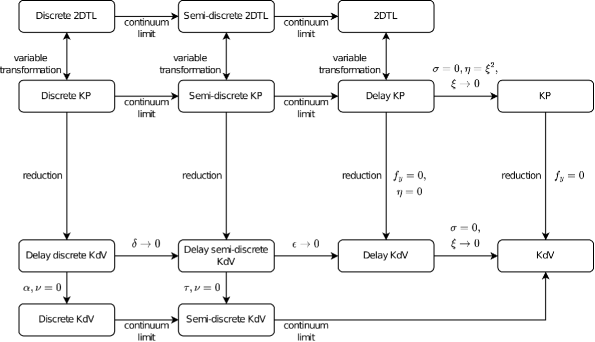
Figure 1: Relationship diagram of the KdV and KP families.

The derivations of the delay LV, delay TL, and delay sG equations were perfectly parallel to the non-delay version [18]. However, some delay soliton equations (such as the delay KdV equation) cannot be obtained by this idea. In this paper, the delay KdV equation succeeded to be obtained by a technique which is not parallel to the non-delay version (as we discussed in Remark 2.7).

This paper and our previous studies [17, 18] mainly focus on proposing delay soliton equations and deriving their soliton solutions. Thus we have not yet revealed many things about them such as the Lax pairs, ultra-discretization, singularity confinement, and relationships to the delay-differential Painlevé equations. In particular, it should be investigated whether delay Painlevé equations are derived by reductions of delay soliton equations. In addition, it remains unclear if the delay soliton equations can model and analyze feedback systems such as traffic flow. We intend to address these problems in future studies.