Stochastic modelling of blob-like plasma filaments in the scrape-off layer: Theoretical foundation
Abstract
A stochastic model for a super-position of uncorrelated pulses with a random distribution of amplitudes, sizes and velocities is presented. The pulses are assumed to move radially with fixed shape and amplitudes decaying exponentially in time due to linear damping. The pulse velocities are taken to be time-independent but randomly distributed. The implications of a distribution of pulse amplitudes, sizes and velocities are investigated. Closed-form expressions for the cumulants and probability density functions for the process are derived in the case of exponential pulses and a discrete uniform distribution of pulse velocities. The results describe many features of the boundary region of magnetically confined plasmas such as high average particle densities, broad and flat radial profiles, and intermittent large-amplitude fluctuations. The stochastic model elucidates how these phenomena are related to the statistical properties of blob-like structures. In particular, the presence of fast pulses generally leads to flattened far scrape-off layer profiles and enhanced intermittency, which amplifies plasma–wall interactions.
I Introduction
Magnetically confined fusion plasmas in toroidal geometry rely on a poloidal divertor topology in order to control plasma exhaust.[1, 2, 3, 4] Plasma entering the scrape-off layer (SOL) from the core will flow along magnetic field lines to the remote divertor chamber, which is specifically designed to handle the exhaust of particles and heat. This is supposed to avoid strong plasma–wall contact in the main chamber, which is located close to the core plasma. However, experiments have shown that cross-field plasma transport is generally significant and may even be dominant, leading to detrimental plasma interactions with the main chamber walls.[1, 2, 3, 4, 5, 6, 7, 8, 9, 10]
Measurements on numerous tokamak devices have demonstrated that as the core plasma density increases, the particle density in the SOL becomes higher and plasma–wall interactions increase.[11, 12, 13, 14, 15, 16, 17, 18, 19, 20, 21, 22, 23, 24, 25, 26, 27, 28, 29, 30, 31, 32, 33, 34, 35, 36, 37, 38, 39, 40, 41, 42, 43, 44, 45, 46, 47, 48, 49, 50] The particle density profile in the SOL typically exhibits a two-layer structure, commonly referred to as a density shoulder. Close to the magnetic separatrix, in the so-called near SOL, it has a steep exponential decay and moderate fluctuation levels. Beyond this region, in the so-called far SOL, the profile has an exponential decay with a much longer scale length. As the core plasma density increases, the profile scale length in the far SOL becomes longer, referred to as profile flattening, and the break point between the near and the far SOL moves radially inwards, referred to as profile broadening. When the empirical discharge density limit is approached, the far SOL profile effectively extends all the way to the magnetic separatrix or even inside it.
The boundary region of magnetically confined plasmas is generally in an inherently fluctuating state. Single point measurements of the particle density in the far SOL reveal frequent occurrence of large-amplitude bursts and relative fluctuation levels of order unity.[21, 22, 23, 24, 25, 26, 27, 28, 29, 30, 31, 32, 33, 34, 35, 36, 37, 38, 39, 40, 41, 42, 43, 44, 45, 46, 47, 48, 49, 50, 51, 52, 53, 54, 55, 56, 57, 58, 59, 60] The large-amplitude fluctuations, identified in the SOL of all tokamaks and in all confinement regimes, are attributed to radial motion of coherent structures through the SOL and towards the main chamber wall. These structures are observed as magnetic-field-aligned filaments of excess particles and heat as compared to the ambient plasma, commonly referred to as blobs.[61, 62, 63, 64, 65, 66, 67, 68, 69, 70, 71, 72, 73, 74, 75] This leads to broad and flat far SOL profiles and enhanced levels of plasma interactions with the main chamber walls that may be an issue for the next generation magnetic confinement experiments.
At the outboard mid-plane region, localized blob-like structures get charge polarized due to vertical magnetic gradient and curvature drifts. The resulting electric field leads to radial motion of the filament structures towards the main chamber wall. The strongly non-linear advection results in an asymmetric shape with a steep front and a trailing wake. Single-point measurements record the filaments as an asymmetric, two-sided exponential pulse function.[45, 46, 47, 48, 49, 50, 51, 52, 53, 54, 55, 56, 57, 58, 59, 60] The radial filament velocity depends on the blob size and amplitude as well as plasma parameters and takes a wide range of values. This dependence has been extensively explored theoretically and by numerical simulations of isolated filament structures in various plasma parameter regimes.[76, 77, 78, 79, 80, 81, 82, 83, 84, 85, 86, 87, 88, 89, 90, 91, 92, 93, 94, 95] Filament velocity scaling properties have also been investigated experimentally, showing correlations with other blob parameters and plasma parameters.[61, 62, 63, 64, 65, 66, 67, 68, 69, 70, 71, 72, 73, 74, 75] It follows that stochastic modelling of the intermittent fluctuations in the SOL must necessarily include a distribution of filament velocities.
In previous experimental investigations based on second-long, single-point measurement data time series, the fundamental statistical properties of the plasma fluctuations in the far SOL have been identified.[45, 46, 47, 48, 49, 50, 51, 52, 53, 54, 55, 56, 57, 58, 59, 60] It has been demonstrated that the fluctuations can be described as a super-position of uncorrelated, exponential pulses with an exponential distribution of pulse amplitudes, referred to as a filtered Poisson process.[96, 97, 98, 99, 100, 101, 102, 103] For such a stochastic process the probability density function is a Gamma distribution with the scale parameter given by the average pulse amplitude and the shape parameter given by the ratio of the average pulse duration and waiting times.[96, 97, 98, 99, 100, 101, 102, 103] Moreover, it follows that the auto-correlation function has an exponential tail and the frequency power spectral density has a Lorentzian shape.[103, 102, 101] Both the underlying assumptions of the model and its predictions are found to be in excellent agreement with experimental measurements.[45, 46, 47, 48, 49, 50, 51, 52, 53, 54, 55, 56, 57, 58, 59, 60]
Recently, the statistical description of single-point measurements was extended to describe the radial variation of the average SOL profile due to the motion of blob-like filament structures with a random distribution of sizes and velocities.[103, 104, 105, 106] This reveals how the average profile and its radial variation depend on the filament statistics. In particular, if all filaments have the same velocity, the radial e-folding length is given by the product of the radial filament velocity and the parallel transit time to the divertor targets. In this presentation, we extended and complement this statistical analysis by a systematic study of randomly distributed filament amplitudes, sizes and velocities, and correlations between these quantities. The filaments are assumed to move radially outwards with fixed shape and amplitudes decaying exponentially in time due to linear damping. The velocities are taken to be time-independent but may be correlated with other filament parameters. The combination of linear damping and a random distribution of velocities is shown to significantly modify the average profiles as well as the fluctuations in the process. The results presented here extend previous work by including predictions for higher-order moments, in particular skewness and flatness profiles. Closed-form analytical expressions are obtained in the case of a discrete uniform distribution of pulse velocities.
This paper is the first in a sequence, presenting extensions of the filtered Poisson process to describe the radial motion of pulses including linear damping due to parallel drainage in the scrape-off layer. This first paper defines the theoretical framework and gives a derivation of all the general results for the case of time-independent pulse velocities and provides closed-form expressions for the relevant statistical averages in the case of a discrete uniform distribution of pulse velocities. Follow-up papers will address various continuous distributions of pulse velocities, cases where the pulse velocity depends on the pulse amplitude, time-dependent pulse velocities, the correlation functions and frequency and wave number spectra of the fluctuations, and extensions to several spatial dimensions.
The organization of this paper is as follows. In Sec. II we present the stochastic model describing a super-position of pulses with a random distribution of and correlations between amplitudes, sizes and velocities. In Sec. III we derive general expressions for the cumulants and discuss how the combination of radial motion and linear damping influences the statistical properties of the fluctuations. In Sec. IV we present closed-form expressions for the radial profile of the lowest order statistical moments and probability distributions for the case of a discrete uniform distribution of pulse velocities. A discussion of the results in the context of blob-like filament structures at the boundary of magnetically confined plasmas is presented in Sec. V and the conclusions and an outlook are given in Sec. VI. The paper is complemented by four appendices. In App. A general results are presented for the case of two-sided exponential pulses. End effects in realizations of the process are considered in App. B. Appendix C discusses limitations on the existence of cumulants. Implications of a discrete uniform distribution of pulse sizes are presented in App. D. Finally, the generalization to a non-uniform discrete velocity distribution is given in App. E.
II Stochastic model
In this section, the stochastic process is presented, describing a super-position of uncorrelated pulses which do not interact with each other. It is demonstrated that this is a generalization of a filtered Poisson process with particularly transparent results obtained for an exponential pulse function.
II.1 Super-position of pulses
Consider the evolution of an individual pulse , which is assumed to follow an advection equation on the form
| (1) |
where is the pulse velocity along the radial axis . The last term on the left-hand side describes linear damping with e-folding time , which is assumed to be constant in time and independent of the pulse parameters. The linear damping originates from the parallel drainage of plasma along the magnetic field lines, hence the subscript . The pulse velocity will in the following be assumed to be positive and time-independent. As initial condition, we take that the pulse is assumed to arrive at the reference position at time ,
| (2) |
where and are the pulse amplitude and size, respectively. The non-dimensional pulse function is taken to be the same for all events and satisfies the normalization constraint
| (3) |
For later reference, we define the integral of the ’th power of the pulse function as
| (4) |
For a non-negative pulse function, it follows that . Applying the method of characteristics to the differential equation (1) leads to the general solution
| (5) |
where the pulse amplitude evolution is determined by
| (6) |
Equation (5) determines the pulse evolution for given amplitude , size and velocity . The pulse moves radially without change in shape but with an amplitude that decays exponentially in time due to the linear damping.
Consider now the stochastic process given by a super-position of uncorrelated and spatially localized pulses,
| (7) |
where each pulse satisfies Eq. (1). In the following, the subscript on the random variables , and will be suppressed when possible for simplicity of notation. Each pulse is located at at the arrival time . All other pulse parameters are assumed to be independent of the arrival times. The arrival times are furthermore assumed to be independent and uniformly distributed on an interval of duration , that is, their probability distribution function is
| (8) |
With these assumptions, the probability that there are exactly pulse arrivals at during any interval of duration is given by the Poisson distribution
| (9) |
where is the average pulse waiting time at the reference position . The average number of pulses in realizations of duration is
| (10) |
where, here and in the following, angular brackets denote the ensemble average of a random variable over all its arguments. From the Poisson distribution, it follows that the waiting time between two subsequent pulses is exponentially distributed. It is emphasized that all pulse parameters and their correlations are specified at the reference position . In particular, the Poisson property of the process is defined for this reference position but does not necessarily hold for other radial positions. This will be discussed further in Sec. III.3 and App. B.
II.2 Exponential pulses
The exponential amplitude modulation due to linear damping in Eq. (6) suggests that particularly simple expressions may be obtained for a similar dependence in the pulse function. We thus consider the case of a one-sided exponential pulse function,
| (11) |
In the following sections, this one-sided exponential pulse function will be used to demonstrate the fundamental properties of the process and in order to calculate closed-form expressions for moments and distribution functions. It should be noted that for exponential pulses, the integral . The generalization of the following results to two-sided exponential pulses is discussed in App. A.
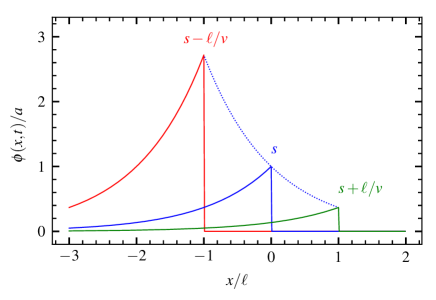
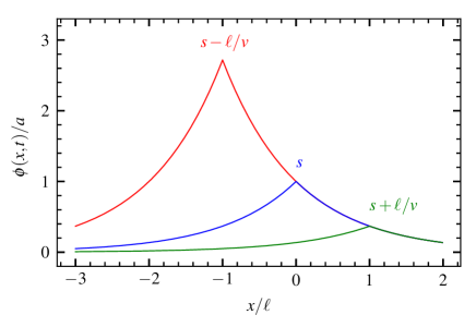
The relevant parameters of the process given by Eq. (II.1) for a one-sided exponential pulse function are presented in Fig. 1. Here the radial variation of the pulse is shown for the time of arrival at as well as one radial transit time before and after this arrival time. Due to linear damping, the amplitude decreases exponentially in time as the pulse moves along the radial axis, indicated by the dotted line in the figure.
At the reference position, , the process is given by
| (12) |
For the exponential pulse function defined by Eq. (11) it is straightforward to show that this process can be written as
| (13) |
where the pulse duration is the harmonic mean of the linear damping time and the radial transit time ,
| (14) |
The average pulse duration is denoted by and is clearly influenced by a distribution of pulse sizes and velocities. In the absence of linear damping, the pulse duration is just the radial transit time, . Further discussions of the pulse duration are given in Sec. III.1.
II.3 Filtered Poisson process
The process at the reference position describes a super-position of uncorrelated, exponential pulses given by Eq. (13). When all pulses have the same duration , the process can be written as a convolution or filtering of the pulse function with a train of delta pulses,[58]
| (15) |
where the forcing is
| (16) |
This is therefore commonly referred to as a filtered Poisson process. More generally, for the process given by Eq. (13) with a random distribution of all pulse parameters, the ratio of the average pulse duration and waiting times,
| (17) |
determines the degree of pulse overlap and is referred to as the intermittency parameter of the process.[96]
In the case of an exponential pulse function and exponentially distributed pulse amplitudes with mean value , which for positive is given by
| (18) |
the raw amplitude moments are and the stationary probability density function for is given by a Gamma distribution with shape parameter and scale parameter . For positive this distribution can be written as[96, 97, 98, 99, 100, 101, 102, 103]
| (19) |
with mean value and variance . The intermittency parameter determines the shape of the distribution, resulting in a high relative fluctuation level as well as skewness and flatness moments in the case of weak pulse overlap for small . The Gamma probability density function holds for any distribution of pulse durations but assumes that the pulse amplitudes and durations are independent.[102, 100]
III Moments of the process
In this section, we present derivations of the mean value, the characteristic function, cumulants and the lowest order statistical moments for a sum of uncorrelated pulses given by Eq. (II.1). Particular attention is devoted to mechanisms for radial variation of moments and intermittency of the process.
III.1 Average radial profile
Let us first consider the average of the process . The arrival times are taken to be independent of the other pulse parameters. Thus, we first perform the average of each pulse over the arrival times,
| (20) |
where the angular brackets denote an average over all amplitudes, sizes and velocities with the subscript suppressed for simplicity of notation. Neglecting end effects by taking the integration limits for to infinity and changing the integration variable to gives
| (21) |
Given that the pulses are uncorrelated, the average of the conditional process with exactly pulses is given by . Therefore, averaging over the number of pulses gives the general result
| (22) | ||||
In the absence of linear damping, the mean value does not depend on the radial coordinate and is given by for any joint distribution between pulse amplitudes, sizes and velocities.
In the case where all pulses have the same velocity, it follows that the average radial profile is exponential with a length scale given by the product of the radial velocity and the linear damping time,
| (23) |
The exponential profile obviously follows from the combination of radial motion and linear damping of the pulses. More generally, it is clear from Eq. (22) that a random distribution of pulse velocities will make the average radial profile non-exponential. This will be further investigated in Sec. IV.
For the exponential pulse function defined by Eq. (11) and any distribution of amplitudes, sizes and velocities, we obtain the average profile
| (24) |
where the pulse duration is given by Eq. (14). In the case of a degenerate distribution of the pulse velocities the average radial profile is exponential,[103, 104, 105]
| (25) |
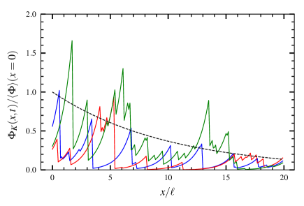
If additionally, the pulse sizes are uncorrelated with the amplitudes, the prefactor is given by with the average pulse duration. Realizations of this process with an exponential amplitude distribution and fixed pulse sizes and velocities are presented in Fig. 2. The pulses cause large-amplitude fluctuations to the average radial profile which will now be quantified with cumulants and higher-order moments.
III.2 Cumulants and moments
The characteristic function for the random variable at the radial position is the Fourier transform of the probability density function and is given by . The characteristic function for a sum of independent random variables is the product of their individual characteristic functions. Since all pulses are by assumption independent, and each of the parameters , and are identically distributed, the characteristic function for the process is given by
| (26) |
where we have defined the characteristic function for an individual pulse as
| (27) |
with given by Eq. (5) and the average is to be taken over arrival times and the other randomly distributed pulse parameters.
The conditional probability distribution function of for fixed is
| (28) |
Using that is Poisson distributed as defined by Eq. (9) we have
| (29) | ||||
The expression inside the last exponential function can be identified as the logarithm of the characteristic function , given by
| (30) |
where the averaging in the last expression is over all pulse amplitudes, sizes and velocities. Neglecting end effects by extending the integration limits over pulse arrivals to infinity and expanding the exponential function we can write
| (31) |
The statistical moments are directly related to the cumulants , which are defined as the coefficients in the expansion of the logarithm of the characteristic function,
| (32) |
A comparison with Eq. (31) gives the cumulants,
| (33) |
Following a similar procedure as for calculating the average radial profile we obtain the general expression for the cumulants,
| (34) |
In the case of a degenerate distribution of pulse velocities, the cumulants decrease exponentially with radius. The exponential profile is clearly modified by a distribution of pulse velocities.
From the cumulants, the lowest order moments of are readily obtained. A formal power series expansion shows that the characteristic function is related to the raw moments ,
| (35) |
The first order cumulant is just the mean value, , while the second order cumulant is the variance of the process, , with
| (36) |
The lowest order centered moments are related to the cumulants by the relations , and . The skewness and flatness moments are defined by
| (37) | ||||
| (38) |
In the following, we will occasionally use a scaled variable defined by
| (39) |
normalized such as to have zero mean and unit standard deviation at all radial positions.
In the absence of linear damping, the cumulants and moments do not depend on the radial coordinate and are given by . For an exponential pulse function, for which , with exponentially distributed amplitudes that are independent of the pulse duration , for which , the cumulants simplify to , where and is the average pulse duration. This is nothing but the cumulants of a Gamma distribution with scale parameter and shape parameter , which is the case discussed in Sec. II.3.
In the case of a degenerate distribution of pulse velocities, the variance is given by
| (40) |
It follows that the relative fluctuation level as well as the skewness and flatness moments do not depend on the radial coordinate. As will be seen in the following section, this is not the case for a broad distribution of pulse velocities.
For an exponential pulse function, the general expression for the cumulants given by Eq. (34) simplifies significantly since the exponential function due to linear damping combines with the pulse function,
| (41) |
where the pulse duration is given by Eq. (14). The factor comes from the integration of the ’th power of the exponential pulse function. In the case of a degenerate distribution of pulse velocities and amplitudes that are uncorrelated with the pulse durations, the cumulants simplify to
| (42) |
where is the pulse duration averaged over the distribution of pulse sizes. It follows that the cumulants and the raw moments decrease exponentially with radius. In particular, the variance is given by
| (43) |
However, the relative fluctuation level and the skewness and flatness moments are all constant as function of radius. Additionally assuming exponentially distributed pulse amplitudes as given by Eq. (18), the cumulants are given by
| (44) |
which are the cumulants of a Gamma distribution with scale parameter and shape parameter . The relative fluctuation level and the skewness and flatness moments then become
| (45) | ||||
| (46) | ||||
| (47) |
The probability density function for is the Gamma distribution given by Eq. (19) with the average radial profile given by . Thus, in the case of a degenerate distribution of pulse velocities, the shape parameter is fixed but the scale parameter for the distribution decreases exponentially with radius. As will be discussed in Sec. III.3, in general, no closed-form expression of the probability distribution function can be obtained in the case of a random distribution of pulse velocities. One notable exception is the case of a discrete uniform distribution of pulse velocities, which will be considered in Sec. IV.
III.3 Filtered Poisson process
A pulse moving with constant velocity will arrive at a radial position at time given by
| (48) |
The arrivals at are assumed to be uniformly distributed on the interval , as described by Eq. (8). In the case of a random distribution of pulse velocities , the arrivals at position are given by a sum of two random variables and therefore the distribution of these arrivals is given by the convolution
| (49) |
where is the distribution of the radial transit times . It follows that the pulse arrivals at radial position are in general not uniformly distributed. A distribution of pulse velocities leads to end effects that influence the arrival time distribution. This is solely an effect of the radial motion and is independent of the linear damping.
In order to determine the arrival time distribution, consider the case of a velocity distribution that is bounded by a minimum velocity and a maximum velocity , which results in a maximum transit time and a minimum transit time , respectively. The probability distribution then vanishes for as well as for , and the integral in Eq. (49) can be rewritten as
| (50) |
Thus, for arrival times such that we obtain
| (51) |
That is, a broad velocity distribution leading to transit times in the interval will result in a distribution of arrival times at the radial position that is uniform on the interval and therefore constitute a Poisson point process. Note that this assumes . In the case of a degenerate distribution of pulse velocities and the pulse arrivals at constitute a Poisson process on the translated interval . For a sufficiently long realization of the process, , end effects can be neglected and the process follows Poisson statistics in the radial domain of interest. Further discussions of end effects and the rate of the process are given in App. B.
As discussed above, a pulse will arrive at position at time . The superposition of pulses at this position can thus be written as
| (52) |
where the pulse amplitudes are given by
| (53) |
with the pulse amplitudes specified at the reference position . Due to the linear damping and time-independent velocities, the pulse amplitudes decrease exponentially with increasing radial position . When the pulse velocities are randomly distributed, the distribution of pulse amplitudes at will be different from the ones specified at the reference position. In particular, the amplitude of slow filaments will decrease substantially with radial position and the process will be dominated by the fast pulses for large since these have shorter radial transit times. As will be discussed below, this correlation between pulse amplitudes and velocities influences the intermittency of the process.
Assuming an exponential pulse function as described by Eq. (11), the exponential amplitude variation can be combined with the pulse function and at the radial position the process can be written as
| (54) |
where the pulse duration is given by Eq. (14). As discussed in Sec. III.3, the pulse arrivals follow a Poisson process when end effects are neglected. The process described by Eq. (54) is therefore a filtered Poisson process generalized to the case of a random distribution of pulse durations. Moreover, this describes how the pulse amplitudes and durations become modified and correlated by a distribution of pulse velocities. Pulses with high (low) velocity will have larger (smaller) amplitudes and shorter (longer) duration times . A distribution of pulse velocities therefore leads to an anti-correlation between amplitudes and durations. The modification of the amplitude distribution and their correlation with pulse durations will be further discussed in Sec. IV.2 for a discrete uniform distribution of pulse velocities.
IV Discrete uniform velocity distribution
The analytical results presented in the previous section show that a distribution of pulse velocities significantly influences both the moments and correlation properties of the stochastic process. Here this will be investigated in detail for the special case of a discrete uniform distribution of pulse velocities, allowing them to take two different values with equal probability,
| (55) |
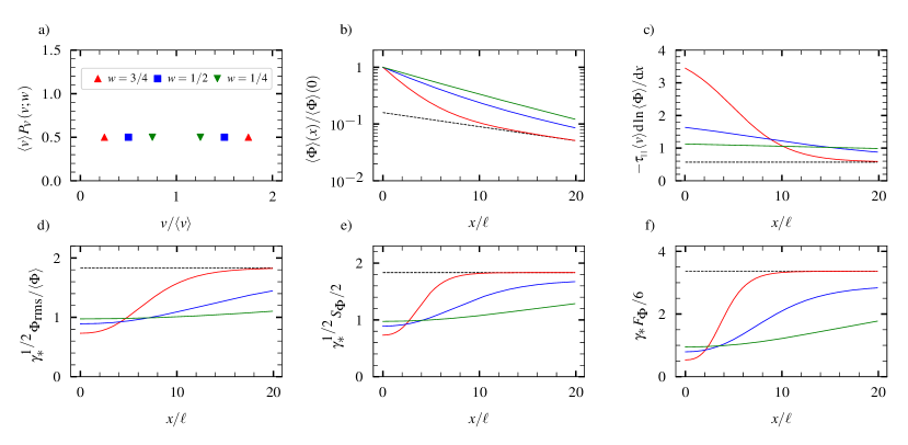
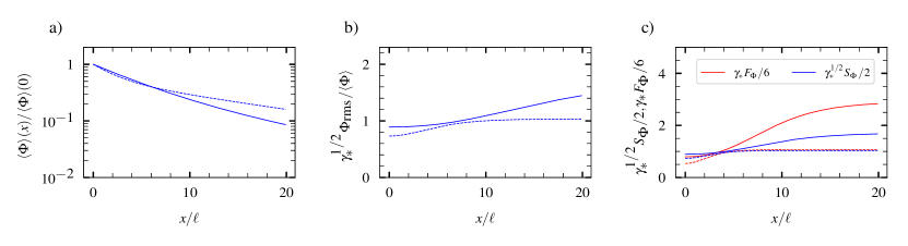
The minimum and maximum velocities are given by and , respectively, is the average velocity and in the range is the width parameter of the distribution. The limit corresponds to the case of a degenerate distribution of pulse velocities. The discrete uniform distribution is presented in Fig. 4a) for various values of the width parameter . In the following, we present the lowest-order statistical moments and probability distributions, and describe how the statistical properties of the process changes with radial position. These theoretical predictions have recently been confirmed by numerical realizations of the process.[106]
Throughout this section, all pulses are assumed to have the same size and we consider for simplicity one-sided exponential pulses with an exponential amplitude distribution at the reference position with mean amplitude . As will be seen, closed-form expressions can be derived for all relevant statistical averages and distributions, allowing to analyze and describe all aspects of the process. The process with a random distribution of pulse velocities will be compared to the standard case with a degenerate distribution of velocities, where all pulses have the same velocity . The pulse duration is then given by
| (56) |
and the process is Gamma distributed with shape parameter
| (57) |
Recall that in this standard case, the average radial profile is exponential, , while higher order normalized moments are radially constant. In particular, the relative fluctuation level is , the skewness is and the flatness is .
IV.1 Radial profiles
The cumulants for the discrete uniform velocity distribution are obtained from Eq. (41) by straightforward integration,
| (58) |
where is the pulse amplitude at the reference position and we have used the notation of a velocity-dependent pulse duration,
| (59) |
The discrete uniform velocity distribution translates into a discrete uniform distribution of pulse durations,
| (60) |
The average pulse duration is given by integration over the discrete distribution,
| (61) |
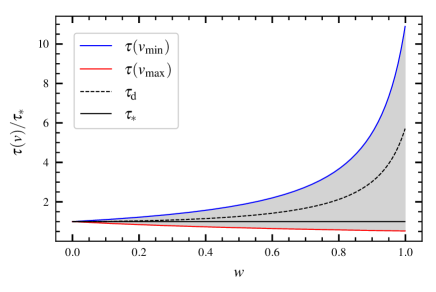
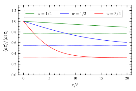
At the reference position the cumulants are given by , showing that determines the degree of pulse overlap and intermittency at this position. Through , the degree of pulse overlap depends on the width of the velocity distribution. The normalized pulse duration is presented in Fig. 3 as a function of the width parameter for . For a fixed average velocity, the average pulse duration increases significantly with the width parameter of the velocity distribution. In fact, in the absence of linear damping, the average pulse duration diverges in the limit . This is due to the cumulative contribution of nearly stagnant pulses. More generally, the width of the velocity distribution is important for determining the average pulse duration and therefore all cumulants at the reference position.
The width of the velocity distribution also influences the radial variation of the cumulants. In the limit the velocity distribution tends to a degenerate distribution, giving the familiar exponential profile with scale length . For , the shorter e-folding length of the first term in Eq. (58) makes this term dominant for negative , while the longer e-folding length of the second term makes this dominant for positive . The cumulants given by Eq. (58) show that there is a breakpoint between the two exponential functions whose radial location is given by their equal contribution. This depends on the strength of the linear damping and the width of the velocity distribution,
| (62) |
It is to be noted that the break point is located at positive values of and decreases with the order of the cumulant. In the limit the breakpoint approaches the origin. Moreover, the radial location of the breakpoint increases with the normalized linear damping time . Indeed, as discussed previously, in the absence of linear damping these profiles are radially constant and there is no break point.
In general, the statistical properties of the process for negative are dominated by the slow pulses due to their long radial transit times and therefore excessively large upstream amplitudes, as described by Eq. (53). The process for a large negative position is effectively a filtered Poisson process given by only the slow pulses,
| (63) |
with the amplitudes given by and the pulse arrivals . This process is Gamma distributed with shape parameter given by . Similarly, the statistical properties of the process for large positive are dominated by the fast pulses since the slow pulses are depleted by the linear damping. Indeed, for a sufficiently large radial position , the process is determined solely by the fast pulses, giving rise to another filtered Poisson process which is given by
| (64) |
with the amplitudes given by and the pulse arrivals . This process is Gamma distributed with shape parameter . The dependence of the average pulse duration on the width of the velocity distribution for these two sub-processes is also presented in Fig. 3, showing how the degree of intermittency varies from far upstream to far downstream of the reference position.
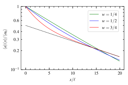
From Eq. (58) it follows that the average radial profile is the sum of two exponential functions,
| (65) |
At the reference position this gives , as expected. The radial profile of the average value , its normalized inverse e-folding length, the relative fluctuation level and the skewness and flatness moments are presented in Fig. 4 for and three different values of the width parameter . All radial profiles are normalized to their value at the reference position for the standard case of a degenerate distribution of pulse velocities corresponding to . The breakpoints for the cumulants given by Eq. (62) are indicated by filled circles in Fig. 4. For small values of , the average profile is nearly exponential and close to that of the reference case, in which all pulses have the same velocity. As expected, the relative fluctuation level, skewness and flatness have weak variation with radial position for small . For a wide separation of pulse velocities, the average profile is steep for small and has a much longer scale length for large , where it is dominated by the fast pulses. Associated with this variation for the average profile is a reduced relative fluctuation level as well as skewness and flatness moments for small , while these quantities increase radially outwards until they saturate at the values associated with the process dominated by the fast pulses, given by the process defined above and indicated by the dashed lines in Fig. 4 for the case . These profiles demonstrate how a distribution of pulse velocities influences the lowest order moments of the process. In particular, both the relative fluctuation level and the skewness and flatness moments may increase significantly above the levels for a degenerate distribution of pulse velocities.
IV.2 Probability distributions
A non-degenerate velocity distribution will change the amplitude distribution at various radial positions as described by Eq. (53). For the discrete uniform velocity distribution, the radial profile of the average amplitude is given by a sum of two exponential functions,
| (66) |
This is presented in Fig. 5 for and three different values of the width parameter . For a narrow velocity distribution, the average amplitude decreases nearly exponentially with radial position with scale length , similar to the standard case where all pulses have the same velocity. For a wide separation of pulse velocities, the average amplitude decreases sharply with radius for small , while for large the profile is exponential and dominated by the fast pulses with scale length . This is demonstrated by the dashed line in Fig. 5, which corresponds to the second term inside the square brackets in Eq. (66).
The probability density function for the pulse amplitudes can be obtained when these are independent of the velocities by using the joint distribution function for the two random variables. The conditional distribution function for the amplitudes at position given the pulse velocity is . Since the pulse amplitudes at are exponentially distributed and change with radial position according to Eq. (53), is an exponential distribution with mean value . Since the pulse velocities and have equal probability , it follows that the probability density function for the pulse amplitudes at position with the appropriate normalization is given by
| (67) |
where we have defined the radial amplitude profile for the fast and slow pulses respectively by
| (68) | ||||
| (69) |
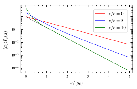
The amplitude distribution is presented in Fig. 6 at various radial positions for the parameters and . The distribution is exponential at , while for large the distribution has a clear bi-exponential behaviour with a much higher probability for small amplitudes associated with the slow pulses. The dashed line in Fig. 6 is the amplitude distribution for the fast pulses, given by the second term in Eq. (67), showing that the tail distribution is due to the fast pulses.
As discussed above, the process for a discrete uniform distribution of pulse velocities can be considered as a sum of the two sub-processes and , each with a degenerate distribution of pulse velocities with values and , respectively. Accordingly, the probability density function for the summed process is the convolution of the probability distribution of the two sub-processes. Each of these two filtered Poisson processes are Gamma distributed with scale parameter given by the average amplitude and shape parameter given by for the two pulse velocities and , where the pulse duration is defined by Eq. (59). The shape and radial variation of the probability density function will depend on the degree of pulse overlap described by , the normalized linear damping time , and the width parameter for the velocity distribution. At the distributions of the two sub-processes have the same scale parameter , which implies that the probability density function for the summed process is itself a Gamma distribution,
| (70) |
with shape parameter . On the other hand, for sufficiently large , the amplitudes of the slow pulses will be depleted due to the linear damping and the process is entirely dominated by the fast pulses, described by Eq. (64). In this case, the probability density function for the process will be another Gamma distribution with scale parameter and shape parameter . For intermediate radial positions, the probability density function is a convolution of two Gamma distributions.
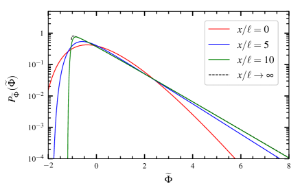
The probability density function for the normalized variable is presented in Fig. 7 for various radial positions and the parameters , and . At the distribution is unimodal with skewness and flatness moments and , respectively, with . Radially outwards the distribution function becomes strongly skewed and has an exponential tail towards large fluctuation amplitudes. This change in the shape of the probability density function is of course fully consistent with the radial profile of the lowest order statistical moments presented in Fig. 4. This demonstrates that a distribution of pulse velocities can lead to significant changes in the probability density function and an increase of the relative fluctuation level and intermittency with radial position. The latter is further emphasized by Fig. 3, indicating how the intermittency parameter for the process at and for the asymptotic process for large varies with the width parameter of the velocity distribution.
For the simple case of a discrete uniform distribution of pulse velocities, the process can readily be interpreted in terms of two sub-processes and corresponding to the two possible velocities as described above. However, as discussed in Sec. III.3, a distribution of pulse velocities gives rise to a change in the amplitude distribution and a correlation between pulse amplitudes and durations, which influences the intermittency of the process. Figure 8 shows the radial variation of the linear correlation between pulse amplitudes and durations, , for and different values of the width parameter . As is clear from Eqs. (53) and (59), an increasing pulse velocity gives large amplitude and shorter duration, resulting in a significant anti-correlation between these quantities. The quantity presented in Fig. 8 can also be interpreted as an effective pulse duration that is weighted with the pulse amplitude. At large radial positions, the process is dominated by the fast pulses, resulting in an effective pulse duration given by , which obviously increases the intermittency of the process.
The radial variation of intermittency in the process is due to the change in amplitude distribution with radius, as described by Eq. (67) and shown in Fig. 6, as well as the linear correlation between pulse amplitudes and durations. In order to separate these, consider the modified filtered Poisson process
| (71) |
where the arrival times are given by Eq. (48), the pulse durations are distributed according to Eq. (60) with the mean value given by Eq. (61), and the amplitudes are distributed according to Eq. (67). This process thus has the same marginal distributions of pulse amplitudes and durations as the original process but with the correlation between amplitudes and durations artificially removed. It is straightforward to calculate the cumulants and the radial profile of the lowest order statistical moments of this modified process. Figure 9 show the radial variation of the lowest order statistical moments for the two processes and for width parameter and normalized linear damping time . For large , the original process has significantly higher relative fluctuation level as well as skewness and flatness moments than the process where the correlations have been removed. This is due to the fact that a wide separation of pulse velocities influences both the pulse amplitudes and durations, and the fast pulses with large amplitudes and short durations dominate the process far downstream.
V Discussion
The statistical properties of a stochastic process given by a super-position of uncorrelated pulses with a random distribution of amplitudes, sizes and velocities have been described. The pulses are assumed to move radially with time-independent velocities and are subject to linear damping, resulting in pulse amplitudes decaying exponentially in time. General results for the cumulants and lowest-order moments of the process have been obtained. When end effects are neglected in realizations of the process and the velocities are time-independent, the rate of pulses remains the same at all radial positions.
In the absence of linear damping, the process is both temporally and spatially homogeneous. Expressions for the cumulants and moments are readily obtained in terms of integrals over the probability distributions. In particular, the cumulants are given by . For an exponential pulse function and exponentially distributed pulse amplitudes independent of the pulse sizes and velocities, the probability density function is a Gamma distribution with scale parameter and shape parameter , where and are the average pulse duration and waiting times, respectively. Any correlation between pulse amplitudes and duration times will modify this probability density function, as discussed in Sec. III.3.
The presence of linear damping drastically modifies the statistical properties of the process, leading to an exponential decay of the pulse amplitudes and therefore radial variation of all statistical averages of the process. In the simple case that all pulses have the same size and velocity, the process results in an exponential radial profile of the cumulants and the lowest order moments with a characteristic scale length given by the product of the pulse velocity and linear damping time, as described by Eq. (34). A broad distribution of pulse velocities leads to non-exponential profiles and a change in the pulse amplitude statistics and their correlation with pulse durations. Low-velocity pulses will undergo significant amplitude decay during their radial motion, resulting in a strongly peaked downstream amplitude distribution. Moreover, there is an anti-correlation between pulse amplitudes and durations and both these mechanisms give rise to increased intermittency of the process.
The special case of exponential pulses allows to combine the effects of linear damping with the pulse function, providing closed-form expression for many of the statistical averages of the process. When all pulses have the same size and velocity, this is a standard filtered Poisson process at any given radial position with mean pulse amplitude given by and pulse duration given by the harmonic mean of the linear damping and radial transit times, as described by Eq. (14) for one-sided pulses and Eq. (75) for two-sided pulses. The probability density function is again a Gamma distribution but with the scale parameter decreasing exponentially with radial position.
The implications of a random distribution of pulse velocities are most clearly exemplified by a discrete uniform distribution, allowing the pulse velocities to take two different values with equal probability. Closed-form expressions have here been derived for all relevant fluctuation statistics. This results in a bi-exponential function for the cumulants and radial profiles, which are dominated by the slow pulses for negative and by the fast pulses for positive . This describes features similar to that typically found in experimental measurements in the scrape-off layer of magnetically confined plasmas, namely a steep near scrape-off layer profile and a flatter far scrape-off layer, as well as a radial increase of the relative fluctuation level and skewness and flatness moments. Accordingly, the probability density function changes shape from a near-normal distribution at the reference position and a strongly skewed Gamma distribution in the far scrape-off layer.
The stochastic model presented here does not describe the formation mechanism for blob structures, only the average radial profile and its fluctuations based on radial motion and linear damping of such structures. In magnetically confined plasmas, the blob structures are generally considered to be formed close to the magnetic separatrix. Once they are formed the blob structures will accelerate and move radially outwards. It should be noted that the case with a wide discrete uniform velocity distribution does indeed describe a steeper near scrape-off layer profile in the region that is dominated by the slow pulses. This resembles the properties of the blob formation region. However, the far scrape-off layer is dominated by the fast pulses, resulting in large-amplitude fluctuations. Additionally, the blob formation process determines the rate of pulses, defined by the average waiting time . This is an input parameter for the stochastic model and its value must be determined by a first-principles based approach.
Characteristic scrape-off layer plasma parameters in medium-sized tokamaks are electron and ion temperatures and a magnetic connection length from the outboard mid-plane to divertor targets of . For a typical blob size of and radial velocity , this gives the normalized linear damping rate , a pulse duration of approximately and a profile scale length for a degenerate distribution of pulse velocities of . This justifies the dominant radial transport parameter used in the analysis presented here and demonstrates that this model is capable to describe strongly flattened far scrape-off layer particle density profiles.
Plasma blobs are three-dimensional, magnetic field-aligned structures which have peak amplitudes at the outboard mid-plane region due to unfavourable curvature in toroidal geometry. The filament temperature and initial extension along the magnetic field may change from one event to another. This motivates the introduction of a random distribution of the linear damping time . The expressions derived for the cumulants in Eqs. (34) and 41 remain valid as far as the statistical average is taken also over the distribution of damping times. The effect of a distribution of on the statistical properties of the process is effectively the same as that of the pulse velocity , since it determines the e-folding length of the cumulants. Thus, a stochastic process with a degenerate velocity distribution but a random distribution of damping times will be very similar to the process discussed above. A positive correlation between pulse velocities and linear damping will further enhance the effect of fast pulses since the profile e-folding length will be larger for those: fast pulses with long damping times will reach the far scrape-off layer without significant amplitude reduction. By contrast, slow pulses with short damping times will have substantial amplitude reduction and contribute little to the far scrape-off layer profile and its fluctuations. Thus, the far scrape-off layer will be highly intermittent and dominated by the fast pulses.
VI Conclusions and outlook
Broad and flat time-average radial profiles of particle density and temperature in the scrape-off layer of magnetically confined plasmas are generally attributed to the radial motion of blob-like filament structures. Simple theoretical descriptions and transport code modelling describe this by means of effective diffusion and convection velocities, neglecting the intermittent and large-amplitude fluctuations of the plasma parameters in the boundary region.[1] Recently, some first attempts at describing both the fluctuations and the time-average radial profiles have been presented.[103, 104, 105] These are based on a stochastic model describing the fluctuations as a super-position of uncorrelated pulses with a random distribution of amplitudes, sizes and velocities.[96, 97, 98, 99, 100, 101, 102, 103]
In this contribution, we have presented the theoretical foundation for a stochastic modelling of blob-like structures in the scrape-off layer, moving radially with a time-independent velocity but subject to linear damping due to drainage along magnetic field lines. General expressions have been derived for the cumulants and lowest order moments for the process in the case of a general distribution of pulse amplitudes, sizes and velocities, as well as correlations between these. Closed-form expressions for an exponential pulse function provide particularly insightful results, clearly demonstrating how a distribution of pulse parameters influences the statistical properties of the process. Even for the simple case of a discrete uniform pulse velocity distribution, many salient features of experimental measurements are recovered by the model, including distinction between near and far scrape-off layer regions, a broad and flat far scrape-off layer profile, radial increase of the relative fluctuation level, and strongly intermittent far scrape-off layer plasma fluctuations.
The stochastic model promises to be a highly valuable framework for analyzing and describing experimental measurements. In particular, imaging data can be used to estimate blob sizes, velocities and amplitudes and correlations between these. Moreover, the model can also be applied to data from first-principles based turbulence simulations of the boundary region in order to describe and understand the relation between blob statistics and resulting time-averaged profiles. Furthermore, the model can be used to validate model simulations against experimental measurement data. In future work, the model presented here will be extended to describe various continuous velocity distributions as well time-varying pulse velocities. In particular, cases where the pulse velocity is given by the instantaneous pulse amplitude will be considered, with specific scaling relationships predicted by theory for isolated plasma filaments.[76, 77, 78, 79, 80, 81, 82, 83, 84, 85, 86, 87, 88, 89, 90, 91, 92, 93, 94, 95]
Acknowledgements
This work was supported by the UiT Aurora Centre Program, UiT The Arctic University of Norway (2020). A. T. was supported by Tromsø Research Foundation under grant number 19_SG_AT. Discussions with O. Paikina and M. Rypdal are gratefully acknowledged.
Appendix A Two-sided exponential pulses
The case of one-sided exponential pulses can readily be generalized to the case of a continuous, two-sided pulse function,
| (72) |
where the spatial pulse asymmetry parameter is in the range . For the pulse function is symmetric, as shown in Fig. 10. It is clear that the two-sided exponential pulse contributes to the mean value of the process at any given position both prior to and after its arrival at this position. The pulse has a steeper leading front than trailing wake for . In the limit this reduces to the simple case of a one-sided exponential pulse function given by Eq. (11). The integral of the ’th power of the pulse function, defined by Eq. (4), is the same as for one-sided pulses, , independent of the pulse asymmetry parameter .
At any radial position the super-position of pulses can be written as
| (73) |
where and is given by Eq. (53). For the two-sided exponential pulse function defined by Eq. (72) it is straightforward to show that this process can be written as
| (74) |
where the pulse duration is given by the sum of the pulse rise and fall times,
| (75) |
and the temporal asymmetry parameter is the ratio of the pulse rise time and duration,
| (76) |
In the limit we obtain the case of a one-sided exponential pulse function with vanishing rise time, , and the pulse duration is the harmonic mean of the linear damping time and the radial transit time given by Eq. (14). In the absence of linear damping, the pulse duration is just the radial transit time, , and the spatial and temporal asymmetry parameters are the same, .
There are some non-trivial criteria for the existence of the mean value and higher-order statistical moments even for a degenerate velocity distribution. From Eq. (22) it is noted that the pulse function must decrease sufficiently rapid and at least exponentially for large in order for the integral over to converge. The reason for this possible divergence is that pulses contribute to the mean value and higher order moments at any radial position prior to their arrival at that position when the pulse function is non-negative ahead of the pulse maximum. To illustrate this, consider the two-sided exponential pulse function given by Eq. (72). The average is finite only if , that is, when the weighted radial transit time is shorter than the linear damping time . Otherwise, the integral over positive diverges.
The radial variation and evolution of a pulse for the marginal case is presented in Fig. 10 for the arrival time as well as one radial transit time before and after the arrival at . When the pulse amplitude decay during the radial transit is so weak that the mean value at any radial position is dominated by the leading front from upstream pulses. This leads to a divergence of the mean value of the process as well as all higher-order moments. Clearly, for and the pulse duration given by Eq. (75) is positive definite. It is to be noted that the requirement must hold for all pulses in the process, so fast and short length scale pulses set the strongest requirement for the asymmetry parameter . For one-sided exponential pulses, there are no such requirements for the existence of the average.
Appendix B End effects and Poisson process
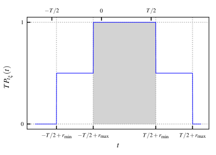
The end effects discussed in Sec. III.3 are clearly illustrated with the example of a discrete uniform distribution of pulse velocities given by Eq. (55). Assuming , the pulse arrival time distribution becomes
| (77) |
This distribution is presented in Fig. 11 for the case in order to emphasize the presence of end effects. As stated in Sec. III.3, the distribution of arrival times is in the range from to . Neglecting end effects by taking the process duration to be much larger than , the arrival times are uniformly distributed at all radial positions considered. However, the interval of uniform arrivals diminishes as becomes arbitrarily small, again revealing issues with low pulse velocities. Nevertheless, we conclude that, except for end effects, the pulse arrivals are uniformly distributed at all radial positions and the stochastic process retains its Poisson property with the same rate at all positions. Moreover, it is straightforward to show that the rate of the process is the same as at the reference position . It should be noted that based on the results presented here, end effects can easily be accounted for in realizations of the process. These arguments for uniform pulse arrival times do not make any assumptions about the pulse function or distributions of the pulse parameters, only that the pulse velocities are time-independent.
Appendix C Existence of cumulants
Low pulse velocities lead to issues with the existence of cumulants and moments of the process. Upon examination of Eqs. (34) and (41) it becomes clear that the expected value of the cumulants may not exist for . In particular, consider for simplicity the case of one-sided exponential pulses, a degenerate distribution of sizes, and velocities with a probability distribution which is independent of the pulse amplitudes. With these assumptions, the -th cumulant becomes
| (78) |
where is the marginal distribution of pulse velocities. The integral over pulse velocities may not converge for negative values of . Notice that the fraction only takes values between and and so does not affect the convergence of the integral. Thus, we examine the convergence of the integral
| (79) |
for which we use absolute value to emphasize that . Making a change of variable defined by and using the relation , the integral can be written as
| (80) |
In order for this integral to converge for any radial position and any cumulant order , the distribution needs to decay faster than exponential for large . Indeed, for is not sufficient, since the integral will diverge for sufficiently large or . Therefore, we require at least a stretched exponential behaviour, , for large for some , or equivalently for for some constant . For most purposes it is sufficient to impose the simpler condition that finite values of the probability distribution should not reach , in other words, there is a minimum velocity such that for .
In summary, care should be taken when using this model to interpret profiles for negative radial positions, . The reason for the divergence of cumulants is the dominant contribution of slow pulses. Indeed, in the case of time-independent pulse velocities, we have from Eq. (6)
| (81) |
where is the pulse location at time . With the amplitudes specified as at the reference position , slow pulses will have excessively large amplitudes for negative , resulting in divergence which first arrests higher order cumulants as they have a stronger dependence on the pulse amplitudes. The same condition for convergence of the cumulants applies to two-sided exponential pulses.
Appendix D Size distribution
For completeness, we present here the results for a discrete uniform distribution of pulse sizes in the case where all pulses have the same velocity. Denoting the width parameter for this distribution by , the pulse size probability density function is given by
| (82) |
where , and . According to Eq. (41), a distribution of pulse sizes does not change the radial variation of the cumulants and moments for exponential pulses. When the pulse sizes are independent of the amplitudes, the cumulants for the discrete uniform distribution are given by
| (83) |
where the average pulse duration is given by
| (84) |
and the size-dependent pulse duration is . Thus, a distribution of pulse sizes does not change the radial variation of the moments. In the absence of linear damping, the pulse duration is given by , independent of the width parameter for the size distribution.
Appendix E Non-uniform discrete velocity distribution
In this Appendix, we present some results obtained for a generalization of the velocity distribution considered in this manuscript. We consider a non-uniform two-velocity distribution,
| (85) |
where in the range is the probability that the velocity attains the value . For this distribution is identical to Eq. (55). The cumulants are a straightforward generalization of Eq. (58),
| (86) |
where each term is weighted with the probability of the given velocity. If the amplitudes of the pulses follow an exponential distribution at , the amplitude distribution at radial position is given by
| (87) |
where as before
| (88) | ||||
| (89) |
This is known as a bi-exponential distribution with coefficients , and . The average amplitude decreases exponentially with radius and is given by .
References
- [1] P. C. Stangeby, “The Plasma Boundary of Magnetic Fusion Devices”, Institute of Physics Publishing (2000).
- [2] W. Fundamenski, “Power Exhaust in Fusion Plasmas”, Cambridge University Press (2014).
- [3] S. Krasheninnikov, A. Smolyakov, and A. Kukushkin, “On the Edge of Magnetic Fusion Devices”, Springer (2020).
- [4] F. Militello, “Boundary Plasma Physics: An Accessible Guide to Transport, Detachment, and Divertor Design”, Springer (2023).
- [5] R. A. Pitts, J. P. Coad, D. P. Coster, G. Federici, W. Fundamenski, J. Horacek, K. Krieger, A. Kukushkin, J. Likonen, G. F. Matthews, M. Rubel, and J. D. Strachan, “Material erosion and migration in tokamaks”, Plasma Physics and Controlled Fusion 47, B303 (2005).
- [6] B. Lipschultz, X. Bonnin, G. Counsell, A. Kallenbach, A. Kukushkin, K. Krieger, A. Leonard, A. Loarte, R. Neu, R. A. Pitts, T. Rognlien, J. Roth, C. Skinner, J. L. Terry, E. Tsitrone, D. Whyte, S. Zweben, N. Asakura, D. Coster, R. Doerner, R. Dux, G. Federici, M. Fenstermacher, W. Fundamenski, P. Ghendrih, A. Herrmann, J. Hu, S. Krasheninnikov, G. Kirnev, A. Kreter, V. Kurnaev, B. Labombard, S. Lisgo, T. Nakano, N. Ohno, H. D. Pacher, J. Paley, Y. Pan, G. Pautasso, V. Philipps, V. Rohde, D. Rudakov, P. Stangeby, S. Takamura, T. Tanabe, Y. Yang, and S. Zhu, “Plasma-surface interaction, scrape-off layer and divertor physics: Implications for ITER”, Nuclear Fusion 47, 1189 (2007).
- [7] J. N. Brooks, J. P. Allain, R. P. Doerner, A. Hassanein, R. Nygren, T. D. Rognlien, and D. G. Whyte, “Plasma-surface interaction issues of an all-metal ITER”, Nuclear Fusion 49, 035007 (2009).
- [8] Y. Marandet, A. Mekkaoui, D. Reiter, P. Börner, P. Genesio, F. Catoire, J. Rosato, H. Capes, L. Godbert-Mouret, M. Koubiti, and R. Stamm, “Transport of neutral particles in turbulent scrape-off layer plasmas”, Nuclear Fusion 51, 083035 (2011).
- [9] G. Birkenmeier, P. Manz, D. Carralero, F. M. Laggner, G. Fuchert, K. Krieger, H. Maier, F. Reimold, K. Schmid, R. Dux, T. Pütterich, M. Willensdorfer, and E. Wolfrum, “Filament transport, warm ions and erosion in ASDEX Upgrade L-modes”, Nuclear Fusion 55, 033018 (2015).
- [10] H. Meyer, T. Eich, M. Beurskens, S. Coda, and A. Hakola, “Overview of progress in European medium sized tokamaks towards an integrated plasma-edge/wall solution”, Nuclear Fusion 57, 102014 (2017).
- [11] N. Asakura, Y. Koide, K. Itami, N. Hosogane, K. Shimizu, S. Tsuji-Iio, S. Sakurai, and A. Sakasai, “SOL plasma profiles under radiative and detached divertor conditions in JT-60U”, Journal of Nuclear Materials 241-243, 559 (1997).
- [12] B. LaBombard, J. A. Goetz, I. Hutchinson, D. Jablonski, J. Kesner, C. Kurz, B. Lipschultz, G. M. McCracken, A. Niemczewski, J. Terry, A. Allen, R. L. Boivin, F. Bombarda, P. Bonoli, C. Christensen, C. Fiore, D. Garnier, S. Golovato, R. Granetz, M. Greenwald, S. Horne, A. Hubbard, J. Irby, D. Lo, D. Lumma, E. Marmar, M. May, A. Mazurenko, R. Nachtrieb, H. Ohkawa, P. O’Shea, M. Porkolab, J. Reardon, J. Rice, J. Rost, J. Schachter, J. Snipes, J. Sorci, P. Stek, Y. Takase, Y. Wang, R. Watterson, J. Weaver, B. Welch, and S. Wolfe, “Experimental investigation of transport phenomena in the scrape-off layer and divertor”, Journal of Nuclear Materials 241-243, 149 (1997).
- [13] B. LaBombard, M. V. Umansky, R. L. Boivin, J. A. Goetz, J. Hughes, B. Lipschultz, D. Mossessian, C. S. Pitcher, and J. L. Terry, “Cross-field plasma transport and main-chamber recycling in diverted plasmas on Alcator C-Mod”, Nuclear Fusion 40, 2041 (2000).
- [14] B. LaBombard, R. L. Boivin, M. Greenwald, J. Hughes, B. Lipschultz, D. Mossessian, C. S. Pitcher, J. L. Terry, and S. J. Zweben, “Particle transport in the scrape-off layer and its relationship to discharge density limit in Alcator C-Mod”, Physics of Plasmas 8, 2107 (2001).
- [15] B. Lipschultz, B. LaBombard, C. S. Pitcher, and R. Boivin, “Investigation of the origin of neutrals in the main chamber of Alcator C-Mod”, Plasma Physics and Controlled Fusion 44, 733 (2002).
- [16] B. Lipschultz, D. Whyte, and B. LaBombard, “Comparison of particle transport in the scrape-off layer plasmas of Alcator C-Mod and DIII-D”, Plasma Physics and Controlled Fusion 47, 1559 (2005).
- [17] D. G. Whyte, B. L. Lipschultz, P. C. Stangeby, J. Boedo, D. L. Rudakov, J. G. Watkins, and W. P. West, “The magnitude of plasma flux to the main-wall in the DIII-D tokamak”, Plasma Physics and Controlled Fusion 47, 1579 (2005).
- [18] D. Carralero, H. W. Müller, M. Groth, M. Komm, J. Adamek, G. Birkenmeier, M. Brix, F. Janky, P. Hacek, S. Marsen, F. Reimold, C. Silva, U. Stroth, M. Wischmeier, and E. Wolfrum, “Implications of high density operation on SOL transport: A multimachine investigation”, Journal of Nuclear Materials 463, 123 (2015).
- [19] F. Militello, L. Garzotti, J. Harrison, J. T. Omotani, R. Scannell, S. Allan, A. Kirk, I. Lupelli, and A. J. Thornton, “Characterisation of the L-mode scrape off layer in MAST: Decay lengths”, Nuclear Fusion 56, 016006 (2016).
- [20] A. Wynn, B. Lipschultz, I. Cziegler, J. Harrison, A. Jaervinen, G. F. Matthews, J. Schmitz, B. Tal, M. Brix, C. Guillemaut, D. Frigione, A. Huber, E. Joffrin, U. Kruzei, F. Militello, A. Nielsen, N. R. Walkden, and S. Wiesen, “Investigation into the formation of the scrape-off layer density shoulder in JET ITER-like wall L-mode and H-mode plasmas”, Nuclear Fusion 58, 056001 (2018).
- [21] G. Y. Antar, S. I. Krasheninnikov, P. Devynck, R. P. Doerner, E. M. Hollmann, J. A. Boedo, S. C. Luckhardt, and R. W. Conn, “Experimental Evidence of Intermittent Convection in the Edge of Magnetic Confinement Devices”, Physical Review Letters 87, 65001 (2001).
- [22] J. A. Boedo, D. Rudakov, R. Moyer, S. Krasheninnikov, D. Whyte, G. McKee, G. Tynan, M. Schaffer, P. Stangeby, P. West, S. Allen, T. Evans, R. Fonck, E. Hollmann, A. Leonard, A. Mahdavi, G. Porter, M. Tillack, and G. Antar, “Transport by intermittent convection in the boundary of the DIII-D tokamak”, Physics of Plasmas 8, 4826 (2001).
- [23] D. L. Rudakov, J. A. Boedo, R. A. Moyer, S. Krasheninnikov, A. W. Leonard, M. A. Mahdavi, G. R. McKee, G. D. Porter, P. C. Stangeby, J. G. Watkins, W. P. West, D. G. Whyte, and G. Antar, “Fluctuation-driven transport in the DIII-D boundary”, Plasma Physics and Controlled Fusion 44, 717 (2002).
- [24] G. Y. Antar, G. Counsell, Y. Yu, B. LaBombard, and P. Devynck, “Universality of intermittent convective transport in the scrape-off layer of magnetically confined devices”, Physics of Plasmas 10, 419 (2003).
- [25] J. A. Boedo, D. L. Rudakov, R. J. Colchin, R. A. Moyer, S. Krasheninnikov, D. G. Whyte, G. R. McKee, G. Porter, M. J. Schaffer, P. C. Stangeby, W. P. West, S. L. Allen, and A. W. Leonard, “Intermittent convection in the boundary of DIII-D”, Journal of Nuclear Materials 313-316, 813 (2003).
- [26] D. L. Rudakov, J. A. Boedo, R. A. Moyer, N. H. Brooks, R. P. Doerner, T. E. Evans, M. E. Fenstermacher, M. Groth, E. M. Hollmann, S. Krasheninnikov, C. J. Lasnier, M. A. Mahdavi, G. R. McKee, A. McLean, P. C. Stangeby, W. R. Wampler, J. G. Watkins, W. P. West, D. G. Whyte, and C. P. Wong, “Far scrape-off layer and near wall plasma studies in DIII-D”, Journal of Nuclear Materials 337-339, 717 (2005).
- [27] G. S. Kirnev, V. P. Budaev, S. A. Grashin, L. N. Khimchenko, and D. V. Sarytchev, “Comparison of plasma turbulence in the low- and high-field Scrape-Off Layers in the T-10 tokamak”, Nuclear Fusion 45, 459 (2005).
- [28] B. LaBombard, J. W. Hughes, D. Mossessian, M. Greenwald, B. Lipschultz, and J. L. Terry, “Evidence for electromagnetic fluid drift turbulence controlling the edge plasma state in the Alcator C-Mod tokamak”, Nuclear Fusion 45, 1658 (2005).
- [29] J. Horacek, R. A. Pitts, and J. P. Graves, “Overview of edge electrostatic turbulence experiments on TCV”, Czechoslovak Journal of Physics 55, 271 (2005).
- [30] O. E. Garcia, J. Horacek, R. A. Pitts, A. H. Nielsen, W. Fundamenski, J. P. Graves, V. Naulin, and J. J. Rasmussen, “Interchange turbulence in the TCV scrape-off layer”, Plasma Physics and Controlled Fusion 48, L1 (2006).
- [31] O. E. Garcia, J. Horacek, R. A. Pitts, A. H. Nielsen, W. Fundamenski, V. Naulin, and J. Juul Rasmussen, “Fluctuations and transport in the TCV scrape-off layer”, Nuclear Fusion 47, 667 (2007).
- [32] O. E. Garcia, R. A. Pitts, J. Horacek, J. Madsen, V. Naulin, A. H. Nielsen, and J. J. Rasmussen, “Collisionality dependent transport in TCV SOL plasmas”, Plasma Physics and Controlled Fusion 49, B47 (2007).
- [33] G. Y. Antar, M. Tsalas, E. Wolfrum, and V. Rohde, “Turbulence during H- and L-mode plasmas in the scrape-off layer of the ASDEX Upgrade tokamak”, Plasma Physics and Controlled Fusion 50, 095012 (2008).
- [34] H. Tanaka, N. Ohno, N. Asakura, Y. Tsuji, H. Kawashima, S. Takamura, and Y. Uesugi, “Statistical analysis of fluctuation characteristics at high- and low-field sides in L-mode SOL plasmas of JT-60U”, Nuclear Fusion 49, 065017 (2009).
- [35] C. Silva, B. Gonçalves, C. Hidalgo, M. A. Pedrosa, W. Fundamenski, M. Stamp, and R. A. Pitts, “Intermittent transport in the JET far-SOL”, Journal of Nuclear Materials 390-391, 355 (2009).
- [36] J. Horacek, J. Adamek, H. W. Muller, J. Seidl, A. H. Nielsen, V. Rohde, F. Mehlmann, C. Ionita, and E. Havlickova, “Interpretation of fast measurements of plasma potential, temperature and density in SOL of ASDEX Upgrade”, Nuclear Fusion 50, 105001 (2010).
- [37] N. Yan, A. H. Nielsen, G. S. Xu, V. Naulin, J. J. Rasmussen, J. Madsen, H. Q. Wang, S. C. Liu, W. Zhang, L. Wang, and B. N. Wan, “Statistical characterization of turbulence in the boundary plasma of EAST”, Plasma Physics and Controlled Fusion 55, 115007 (2013).
- [38] D. Carralero, G. Birkenmeier, H. W. Müller, P. Manz, P. Demarne, S. H. Müller, F. Reimold, U. Stroth, M. Wischmeier, and E. Wolfrum, “An experimental investigation of the high density transition of the scrape-off layer transport in ASDEX Upgrade”, Nuclear Fusion 54, 123005 (2014).
- [39] D. Carralero, J. Madsen, S. A. Artene, M. Bernert, G. Birkenmeier, T. Eich, G. Fuchert, F. Laggner, V. Naulin, P. Manz, N. Vianello, and E. Wolfrum, “A study on the density shoulder formation in the SOL of H-mode plasmas”, Nuclear Materials and Energy 12, 1189 (2017).
- [40] N. Vianello, C. Tsui, C. Theiler, S. Allan, J. Boedo, B. Labit, H. Reimerdes, K. Verhaegh, W. A. J. Vijvers, N. Walkden, S. Costea, J. Kovacic, C. Ionita, V. Naulin, A. H. Nielsen, J. J. Rasmussen, B. Schneider, R. Schrittwieser, M. Spolaore, D. Carralero, J. Madsen, B. Lipschultz, F. Militello, T. T. Team, and T. E. M. Team, “Modification of SOL profiles and fluctuations with line-average density and divertor flux expansion in TCV”, Nuclear Fusion 57, 116014 (2017).
- [41] D. Carralero, M. Siccinio, M. Komm, S. A. Artene, F. A. D’Isa, J. Adamek, L. Aho-Mantila, G. Birkenmeier, M. Brix, G. Fuchert, M. Groth, T. Lunt, P. Manz, J. Madsen, S. Marsen, H. W. Müller, U. Stroth, H. J. Sun, N. Vianello, M. Wischmeier, and E. Wolfrum, “Recent progress towards a quantitative description of filamentary SOL transport”, Nuclear Fusion 57, 056044 (2017).
- [42] R. Kube, O. E. Garcia, A. Theodorsen, A. Q. Kuang, B. LaBombard, J. L. Terry, and D. Brunner, “Statistical properties of the plasma fluctuations and turbulent cross-field fluxes in the outboard mid-plane scrape-off layer of Alcator C-Mod”, Nuclear Materials and Energy 18, 193 (2019).
- [43] N. Vianello, D. Carralero, C. K. Tsui, V. Naulin, M. Agostini, I. Cziegler, B. Labit, C. Theiler, E. Wolfrum, D. Aguiam, S. Allan, M. Bernert, J. Boedo, S. Costea, H. D. Oliveira, O. Fevrier, J. Galdon-Quiroga, G. Grenfell, A. Hakola, C. Ionita, H. Isliker, A. Karpushov, J. Kovacic, B. Lipschultz, R. Maurizio, K. McClements, F. Militello, A. H. Nielsen, J. Olsen, J. J. Rasmussen, T. Ravensbergen, H. Reimerdes, B. Schneider, R. Schrittwieser, E. Seliunin, M. Spolaore, K. Verhaegh, J. Vicente, N. Walkden, W. Zhang, the ASDEX Upgrade Team, the TCV Team, and the EUROfusion MST1 Team, “Scrape-off layer transport and filament characteristics in high-density tokamak regimes”, Nuclear Fusion 60, 016001 (2020).
- [44] A. Stagni, N. Vianello, C. K. Tsui, C. Colandrea, S. Gorno, M. Bernert, J. A. Boedo, D. Brida, G. Falchetto, A. Hakola, G. Harrer, H. Reimerdes, C. Theiler, E. Tsitrone, N. Walkden, the TCV Team, and the EUROfusion MST1 Team, “Dependence of scrape-off layer profiles and turbulence on gas fuelling in high density H-mode regimes in TCV”, Nuclear Fusion 62, 096031 (2022).
- [45] A. Theodorsen, O. E. Garcia, J. Horacek, R. Kube, and R. A. Pitts, “Scrape-off layer turbulence in TCV: Evidence in support of stochastic modelling”, Plasma Physics and Controlled Fusion 58, 044006 (2016).
- [46] O. E. Garcia, R. Kube, A. Theodorsen, J. G. Bak, S. H. Hong, H. S. Kim, the KSTAR Project Team, and R. A. Pitts, “SOL width and intermittent fluctuations in KSTAR”, Nuclear Materials and Energy 12, 36 (2017).
- [47] N. R. Walkden, A. Wynn, F. Militello, B. Lipschultz, G. Matthews, C. Guillemaut, J. Harrison, D. Moulton, and JET Contributors, “Interpretation of scrape-off layer profile evolution and first-wall ion flux statistics on JET using a stochastic framework based on fillamentary motion”, Plasma Phys. Control. Fusion 59, 085009 (2017).
- [48] A. Q. Kuang, B. LaBombard, D. Brunner, O. E. Garcia, R. Kube, and A. Theodorsen, “Plasma fluctuations in the scrape-off layer and at the divertor target in Alcator C-Mod and their relationship to divertor collisionality and density shoulder formation”, Nuclear Materials and Energy 19, 295 (2019).
- [49] R. Kube, A. Theodorsen, O. E. Garcia, D. Brunner, B. Labombard, and J. L. Terry, “Comparison between mirror Langmuir probe and gas-puff imaging measurements of intermittent fluctuations in the Alcator C-Mod scrape-off layer”, Journal of Plasma Physics 86, 905860519 (2020).
- [50] M. Zurita, W. A. Hernandez, C. Crepaldi, F. A. C. Pereira, and Z. O. Guimaraes-Filho, “Stochastic modeling of plasma fluctuations with bursts and correlated noise in TCABR”, Physics of Plasmas 29, 052303 (2022).
- [51] O. E. Garcia, I. Cziegler, R. Kube, B. LaBombard, and J. L. Terry, “Burst statistics in Alcator C-Mod SOL turbulence”, Journal of Nuclear Materials 438, S180 (2013).
- [52] O. E. Garcia, S. M. Fritzner, R. Kube, I. Cziegler, B. Labombard, and J. L. Terry, “Intermittent fluctuations in the Alcator C-Mod scrape-off layer”, Physics of Plasmas 20, 055901 (2013).
- [53] O. E. Garcia, J. Horacek, and R. A. Pitts, “Intermittent fluctuations in the TCV scrape-off layer”, Nuclear Fusion 55, 062002 (2015).
- [54] R. Kube, A. Theodorsen, O. E. Garcia, B. Labombard, and J. L. Terry, “Fluctuation statistics in the scrape-off layer of Alcator C-Mod”, Plasma Physics and Controlled Fusion 58, 054001 (2016).
- [55] A. Theodorsen, O. E. Garcia, R. Kube, B. LaBombard, and J. L. Terry, “Relationship between frequency power spectra and intermittent, large-amplitude bursts in the Alcator C-Mod scrape-off layer”, Nuclear Fusion 57, 114004 (2017).
- [56] R. Kube, O. E. Garcia, A. Theodorsen, D. Brunner, A. Q. Kuang, B. LaBombard, and J. L. Terry, “Intermittent electron density and temperature fluctuations and associated fluxes in the Alcator C-Mod scrape-off layer”, Plasma Physics and Controlled Fusion 60, 065002 (2018).
- [57] O. E. Garcia, R. Kube, A. Theodorsen, B. LaBombard, and J. L. Terry, “Intermittent fluctuations in the Alcator C-Mod scrape-off layer for ohmic and high confinement mode plasmas”, Physics of Plasmas 25, 056103 (2018).
- [58] A. Theodorsen, O. E. Garcia, R. Kube, B. Labombard, and J. L. Terry, “Universality of Poisson-driven plasma fluctuations in the Alcator C-Mod scrape-off layer”, Physics of Plasmas 25, 122309 (2018).
- [59] A. Bencze, M. Berta, A. Buzás, P. Hacek, J. Krbec, and M. Szutyányi, “Characterization of edge and scrape-off layer fluctuations using the fast Li-BES system on COMPASS”, Plasma Physics and Controlled Fusion 61, 085014 (2019).
- [60] S. J. Zweben, M. Lampert, and J. R. Myra, “Temporal structure of blobs in NSTX”, Physics of Plasmas 29, 072504 (2022).
- [61] S. J. Zweben, “Search for coherent structure within tokamak plasma turbulence”, Physics of Fluids 28, 974 (1984).
- [62] S. J. Zweben, D. P. Stotler, J. L. Terry, B. Labombard, M. Greenwald, M. Muterspaugh, C. S. Pitcher, K. Hallatschek, R. J. Maqueda, B. Rogers, J. L. Lowrance, V. J. Mastrocola, and G. F. Renda, “Edge turbulence imaging in the Alcator C-Mod tokamak”, Physics of Plasmas 9, 1981 (2002).
- [63] J. L. Terry, S. J. Zweben, K. Hallatschek, B. LaBombard, R. J. Maqueda, B. Bai, C. J. Boswell, M. Greenwald, D. Kopon, W. M. Nevins, C. S. Pitcher, B. N. Rogers, D. P. Stotler, and X. Q. Xu, “Observations of the turbulence in the scrape-off-layer of Alcator C-Mod and comparisons with simulation”, Physics of Plasmas 10, 1739 (2003).
- [64] S. J. Zweben, R. J. Maqueda, D. P. Stotler, A. Keesee, J. Boedo, C. E. Bush, S. M. Kaye, B. LeBlanc, J. L. Lowrance, V. J. Mastrocola, R. Maingi, N. Nishino, G. Renda, D. W. Swain, and J. B. Wilgen, “High-speed imaging of edge turbulence in NSTX”, Nuclear Fusion 44, 134 (2004).
- [65] J. L. Terry, S. J. Zweben, O. Grulke, M. J. Greenwald, and B. LaBombard, “Velocity fields of edge/Scrape-Off-Layer turbulence in Alcator C-Mod”, Journal of Nuclear Materials 337-339, 322 (2005).
- [66] O. Grulke, J. L. Terry, B. LaBombard, and S. J. Zweben, “Radially propagating fluctuation structures in the scrape-off layer of Alcator C-Mod”, Physics of Plasmas 13, 012306 (2006).
- [67] J. L. Terry, S. J. Zweben, M. V. Umansky, I. Cziegler, O. Grulke, B. LaBombard, and D. P. Stotler, “Spatial structure of scrape-off-layer filaments near the midplane and X-point regions of Alcator-C-Mod”, Journal of Nuclear Materials 390-391, 339 (2009).
- [68] N. Ben Ayed, A. Kirk, B. Dudson, S. Tallents, R. G. Vann, and H. R. Wilson, “Inter-ELM filaments and turbulent transport in the Mega-Amp Spherical Tokamak”, Plasma Physics and Controlled Fusion 51, 035016 (2009).
- [69] R. J. Maqueda, D. P. Stotler, and S. J. Zweben, “Intermittency in the scrape-off layer of the National Spherical Torus Experiment during H-mode confinement”, Journal of Nuclear Materials 415, S459 (2011).
- [70] M. Agostini, J. L. Terry, P. Scarin, and S. J. Zweben, “Edge turbulence in different density regimes in Alcator C-Mod experiment”, Nuclear Fusion 51, 053020 (2011).
- [71] S. Banerjee, H. Zushi, N. Nishino, K. Hanada, S. K. Sharma, H. Honma, S. Tashima, T. Inoue, K. Nakamura, H. Idei, M. Hasegawa, and A. Fujisawa, “Statistical features of coherent structures at increasing magnetic field pitch investigated using fast imaging in QUEST”, Nuclear Fusion 52, 123016 (2012).
- [72] R. Kube, O. E. Garcia, B. LaBombard, J. L. Terry, and S. J. Zweben, “Blob sizes and velocities in the Alcator C-Mod scrape-off layer”, Journal of Nuclear Materials 438, S505 (2013).
- [73] O. Grulke, J. L. Terry, I. Cziegler, B. Labombard, and O. E. Garcia, “Experimental investigation of the parallel structure of fluctuations in the scrape-off layer of Alcator C-Mod”, Nuclear Fusion 54, 043012 (2014).
- [74] G. Fuchert, G. Birkenmeier, D. Carralero, T. Lunt, P. Manz, H. W. Müller, B. Nold, M. Ramisch, V. Rohde, and U. Stroth, “Blob properties in L- and H-mode from gas-puff imaging in ASDEX upgrade”, Plasma Physics and Controlled Fusion 56, 125001 (2014).
- [75] S. J. Zweben, J. R. Myra, W. M. Davis, D. A. D’Ippolito, T. K. Gray, S. M. Kaye, B. P. LeBlanc, R. J. Maqueda, D. A. Russell, and D. P. Stotler, “Blob structure and motion in the edge and SOL of NSTX”, Plasma Physics and Controlled Fusion 58, 044007 (2016).
- [76] S. I. Krasheninnikov, “On scrape off layer plasma transport”, Physics Letters A 283, 368 (2001).
- [77] D. A. D’Ippolito, J. R. Myra, and S. I. Krasheninnikov, “Cross-field blob transport in tokamak scrape-off-layer plasmas”, Physics of Plasmas 9, 222 (2002).
- [78] N. Bian, S. Benkadda, J. V. Paulsen, and O. E. Garcia, “Blobs and front propagation in the scrape-off layer of magnetic confinement devices”, Physics of Plasmas 10, 671 (2003).
- [79] O. E. Garcia, N. H. Bian, V. Naulin, A. H. Nielsen, and J. J. Rasmussen, “Mechanism and scaling for convection of isolated structures in nonuniformly magnetized plasmas”, Physics of Plasmas 12, 090701 (2005).
- [80] O. E. Garcia, N. H. Bian, and W. Fundamenski, “Radial interchange motions of plasma filaments”, Physics of Plasmas 13, 082309 (2006).
- [81] J. R. Myra, D. A. Russell, and D. A. D’Ippolito, “Collisionality and magnetic geometry effects on tokamak edge turbulent transport. I. A two-region model with application to blobs”, Physics of Plasmas 13, 112502 (2006).
- [82] D. A. D’Ippolito, J. R. Myra, and S. J. Zweben, “Convective transport by intermittent blob-filaments: Comparison of theory and experiment”, Physics of Plasmas 18, 060501 (2011).
- [83] J. Madsen, O. E. Garcia, J. Strk Larsen, V. Naulin, A. H. Nielsen, and J. J. Rasmussen, “The influence of finite Larmor radius effects on the radial interchange motions of plasma filaments”, Physics of Plasmas 18, 112504 (2011).
- [84] R. Kube and O. E. Garcia, “Velocity scaling for filament motion in scrape-off layer plasmas”, Physics of Plasmas 18, 102314 (2011).
- [85] D. Higgins, B. Hnat, A. Kirk, P. Tamain, and N. Ben Ayed, “Determining advection mechanism of plasma filaments in the scrape-off layer of MAST”, Plasma Physics and Controlled Fusion 54, 015002 (2012).
- [86] P. Manz, D. Carralero, G. Birkenmeier, H. W. Müller, S. H. Müller, G. Fuchert, B. D. Scott, and U. Stroth, “Filament velocity scaling laws for warm ions”, Physics of Plasmas 20, 102307 (2013).
- [87] F. D. Halpern, A. Cardellini, P. Ricci, S. Jolliet, J. Loizu, and A. Mosetto, “Three-dimensional simulations of blob dynamics in a simple magnetized torus”, Physics of Plasmas 21, 022305 (2014).
- [88] L. Easy, F. Militello, J. Omotani, B. Dudson, E. Havlickova, P. Tamain, V. Naulin, and A. H. Nielsen, “Three dimensional simulations of plasma filaments in the scrape off layer: A comparison with models of reduced dimensionality”, Physics of Plasmas 21, 122515 (2014).
- [89] L. Easy, F. Militello, J. Omotani, N. R. Walkden, and B. Dudson, “Investigation of the effect of resistivity on scrape off layer filaments using three-dimensional simulations”, Physics of Plasmas 23, 012512 (2016).
- [90] M. Held, M. Wiesenberger, J. Madsen, and A. Kendl, “The influence of temperature dynamics and dynamic finite ion Larmor radius effects on seeded high amplitude plasma blobs”, Nuclear Fusion 56, 126005 (2016).
- [91] H. L. Pécseli, D. S. Sortland, and O. E. Garcia, “A solvable blob-model for magnetized plasmas”, Plasma Physics and Controlled Fusion 58, 104002 (2016).
- [92] R. Kube, O. E. Garcia, and M. Wiesenberger, “Amplitude and size scaling for interchange motions of plasma filaments”, Physics of Plasmas 23, 122302 (2016).
- [93] N. R. Walkden, L. Easy, F. Militello, and J. T. Omotani, “Dynamics of 3D isolated thermal filaments”, Plasma Physics and Controlled Fusion 58, 115010 (2016).
- [94] M. Wiesenberger, M. Held, R. Kube, and O. E. Garcia, “Unified transport scaling laws for plasma blobs and depletions”, Physics of Plasmas 24, 064502 (2017).
- [95] A. Ross, A. Stegmeir, P. Manz, D. Groselj, W. Zholobenko, D. Coster, and F. Jenko, “On the nature of blob propagation and generation in the large plasma device: Global GRILLIX studies”, Physics of Plasmas 26, 102308 (2019).
- [96] O. E. Garcia, “Stochastic modeling of intermittent scrape-off layer plasma fluctuations”, Physical Review Letters 108, 265001 (2012).
- [97] R. Kube and O. E. Garcia, “Convergence of statistical moments of particle density time series in scrape-off layer plasmas”, Physics of Plasmas 22, 012502 (2015).
- [98] A. Theodorsen and O. E. Garcia, “Level crossings, excess times, and transient plasma-wall interactions in fusion plasmas”, Physics of Plasmas 23, 040702 (2016).
- [99] A. Theodorsen and O. E. Garcia, “Level crossings and excess times due to a superposition of uncorrelated exponential pulses”, Physical Review E 97, 012110 (2018).
- [100] A. Theodorsen and O. E. Garcia, “Probability distribution functions for intermittent scrape-off layer plasma fluctuations”, Plasma Physics and Controlled Fusion 60, 034006 (2018).
- [101] A. Theodorsen, O. E. Garcia, and M. Rypdal, “Statistical properties of a filtered Poisson process with additive random noise: Distributions, correlations and moment estimation”, Physica Scripta 92, 054002 (2017).
- [102] O. E. Garcia and A. Theodorsen, “Auto-correlation function and frequency spectrum due to a super-position of uncorrelated exponential pulses”, Physics of Plasmas 24, 032309 (2017).
- [103] O. E. Garcia, R. Kube, A. Theodorsen, and H. L. Pécseli, “Stochastic modelling of intermittent fluctuations in the scrape-off layer: Correlations, distributions, level crossings, and moment estimation”, Physics of Plasmas 23, 052308 (2016).
- [104] F. Militello and J. T. Omotani, “Scrape off layer profiles interpreted with filament dynamics”, Nuclear Fusion 56, 104004 (2016).
- [105] F. Militello and J. T. Omotani, “On the relation between non-exponential scrape off layer profiles and the dynamics of filaments”, Plasma Physics and Controlled Fusion 58, 125004 (2016).
- [106] O. Paikina, “Stochastic modelling and numerical simulations of radial filament motion and average profiles at the boundary of fusion plasmas”, Master thesis at UiT, The Arctic University of Norway (2022).