The burst mode of accretion in massive star formation with stellar inertia

Abstract

The burst mode of accretion in massive star formation is a scenario linking the initial gravitational collapse of parent pre-stellar cores to the properties of their gravitationally unstable discs and of their accretion-driven bursts. In this study, we present a series of high-resolution 3D radiation-hydrodynamics numerical simulations for young massive stars formed out of collapsing $100\,\rm M_{\odot}$ molecular cores spinning with several values of the ratio of rotational-to-gravitational energies $\beta=5\%$–$9\%$. The models include the indirect gravitational potential caused by disc asymmetries. We find that this modifies the barycenter of the disc, causing significant excursions of the central star position, which we term stellar wobbling. The stellar wobbling slows down and protracts the development of gravitational instability in the disc, reducing the number and magnitude of the accretion-driven bursts undergone by the young massive stars, whose properties are in good agreement with that of the burst monitored from the massive protostar M17 MIR. Including stellar wobbling is therefore important for accurate modeling disc structures. Synthetic ALMA interferometric images in the millimeter waveband show that the outcomes of efficient gravitational instability such as spiral arms and gaseous clumps can be detected for as long as the disc is old enough and has already entered the burst mode of accretion.

1 Introduction

The burst mode of accretion in star formation is a model proposed to explain the main accretion phase of low-mass stars. In this model, gaseous clumps formed via disk gravitational fragmentation migrate inwards and trigger accretion bursts when tidally destroyed in the vicinity of the star  (Vorobyov & Basu, 2006, 2010, 2015; Machida et al., 2011; Nayakshin & Lodato, 2012; Zhao et al., 2018; Vorobyov et al., 2018). The burst mode of accretion links together several distinct phases experienced by young stars, starting from the initial free-fall collapse of cold pre-stellar cores, through the main accretion phase when a notable fraction of the final stellar mass is acquired during bursts, and finally to the T-Tauri phase, in which the characteristics of young stars may still be affected by the earlier burst phase (Baraffe et al., 2012; Vorobyov et al., 2017; Elbakyan et al., 2019). In this picture, the infall of gas from the collapsing protostellar core plays a key role, replenishing the material lost by the disc during accretion bursts, sustaining the disk in the gravitationally unstable stage and developing disc substructures such as spiral arms and fragments. The burst mode of accretion can resolve the so-called ”luminosity problem” (Kenyon et al., 1990; Kenyon & Hartmann, 1990, 1995; Dunham & Vorobyov, 2012), and the burst characteristics are in accordance with the FU-Orionis-type stars (Vorobyov & Basu, 2015).

A scaling relationship between star-forming mechanisms of low- and high-mass stars has been suspected for decades (Fuente et al., 2001; Testi, 2003; Cesaroni et al., 2006; Johnston et al., 2013), Observations of bipolar H ii  regions and/or jets in the surroundings of young high-mass stars (Cunningham et al., 2009; Caratti o Garatti et al., 2015; Burns et al., 2017; Burns, 2018; Reiter et al., 2017; Purser et al., 2018; Samal et al., 2018; Boley et al., 2019; Zinchenko et al., 2019; Goddi et al., 2020; Purser et al., 2021) provided clues and signatures in its favour. This has been strengthened by the detection of a first luminous flare from the high-mass protostar S255IR-NIRS3 (Caratti o Garatti et al., 2017), and by many others, both in the infrared and by maser emission, in the following years (Moscadelli et al., 2017; Szymczak et al., 2018; Brogan et al., 2018; MacLeod et al., 2018; Liu et al., 2018; Hunter et al., 2017; Proven-Adzri et al., 2019; Lucas et al., 2020; Chen et al., 2020; Olguin et al., 2020; Chen et al., 2020; Burns et al., 2020; Chen et al., 2021; Stecklum et al., 2021; Hunter et al., 2021). Additionally, the discovery, in radiation-hydrodynamics numerical simulations, of processes for the formation of high-mass stars such as accretion-driven outbursts, similar to that of their low-mass counterparts, suggested that the burst mode of accretion in star formation also applies to higher-mass objects (Meyer et al., 2017).

It has successively been found that gaseous clumps in accretion discs surrounding young high-mass stars have pressure and temperature ($>2000\,\rm K$) consistent with the dissociation of molecular hydrogen, meaning that disc fragmentation is also at the origin of the formation of spectroscopic protobinaries (Meyer et al., 2018), see also Oliva & Kuiper (2020). The observability of these nascent binaries has been demonstrated by means of synthetic alma interferometric observations (Meyer et al., 2019). Further studies showed that massive young stellar objects accrete most of their mass within high-magnitude accretion-driven outbursts, taking place during a very short fraction of their pre-main-sequence life (Meyer et al., 2019). During the burst itself, the accretion rate sharply increases, generating a swelling of the protostellar radius, which, in its turn, provokes rapid excursions to the cold part of the Herzsprung-Russell diagram and triggers the intermittency of the irradiation fluxes filling the H ii  region of a young high-mass star (Meyer et al., 2019). Lastly, a parameter study exploring the properties and burst characteristics of a large collection of models for the formation of massive young stellar objects concluded that no massive protostars should form without bursts, which span over a bimodal distribution of short ($\sim 1-10\,\rm yr$) and long ($\sim 10^{3}-10^{4}\,\rm yr$) flares (Meyer et al., 2021), see also Elbakyan et al. (2021).

Gravitation-hydrodynamics naturally includes the gravitational interaction experienced by the substructures developed in the fragmenting accretion discs forming around young stars. Consequently, when the density field of an accretion disc is not described by a symmetric pattern because of the presence of irregular spiral arms and/or (migrating) gaseous clumps, the center of mass of the disc is not anymore coinciding with that of the location of the star. This is particularly true in the case of massive discs forming around high-mass protostars (Meyer et al., 2018). The gravitational interaction between the disc and the star consequently generates an acceleration and a displacement of the protostar as a result of total gravitational force of the disc operating onto the young star. While such a mechanism is intrinsically taken into account in grid-based simulations in Cartesian coordinates (Krumholz et al., 2007b; Seifried et al., 2011; Klassen et al., 2016; Rosen et al., 2019) and Lagrangian models (Springel, 2010), it is often neglected in grid-based models using a spherical, cylindrical or polar coordinate system in which the star is fixed at the coordinate origin (Vorobyov & Basu, 2006; Oliva & Kuiper, 2020).

A number of studies on planet and low-mass star formation have not taken into account this gravitational backaction of the disc onto the star (Tanaka et al., 2002; Pickett et al., 2003; Tanaka & Ward, 2004; Ou et al., 2007; Boley et al., 2007; Tsukamoto & Machida, 2011; Fung & Artymowicz, 2014; Szulágyi et al., 2014; Zhu & Stone, 2014; Lin, 2015) while some other studies did (Regály & Vorobyov, 2017). There, the star-disc barycenter and the geometrical grid center are displaced with respect to each other, in response to the gravitational force of the disc mass exerted onto the protostar, and it provokes a motion of the central star through the disc. A solution to this problem, accounting for the intrinsic singularity present at the coordinate origin of curvelinear coordinate systems, consists in time-dependently displacing the whole disc in responce to an acceleration that the star experiences as a result of disc gravity force. This so-called non-inertial frame of reference, which considers the gravitational response to the disc of the stellar motion, has been introduced in Michael & Durisen (2010a).

We hereby continue our numerical investigation of the burst mode of accretion in massive star formation, by performing high spatial resolution simulations of radiation-hydrodynamical disc models for several initial rotation rates of the molecular pre-stellar core (Meyer et al., 2017). The numerical setup is augmented with the physics of stellar wobbling (Regály & Vorobyov, 2017). We measure from our simulations, both the physical properties of the accretion discs, as well as the characteristics of the accretion-driven outbursts generated by the star-disc system (Meyer et al., 2017, 2018; Meyer et al., 2021). We further discuss our results in the context of the observational appearance of the accretion discs, by performing synthetic interferometric images as seen by the Atacama Large Millimeter/submillimeter Array (alma) when operating at band 6 ($1.2\,\rm mm$). Beyond the confirmation of the observability of the disc of massive young stellar objects (Krumholz et al., 2007a; Jankovic et al., 2019; Meyer et al., 2019), these synthetic observables reveal how the outcomes of gravitational instability should look in realistic discs.

The outline of this study is organised as follows. In Section 2 we present the numerical methods for both the disc and the indirect potential that we use to model the circumstellar medium of young massive stars. In Section 3 we show the effects of the young star’s motion onto the evolution of its circumstellar disc and on the properties of its pre-main-sequence accretion bursts. The caveats of our results are discussed in Section 4, together with the effect of stellar motion on interferometric emission. We conclude in Section 5.

2 Method

In this section we present the methodology used to perform our radiation-hydrodynamical simulations of accretion discs surrounding massive young stellar objects.

2.1 Initial conditions

The simulations in this study are initialised with a three-dimensional, rotating pre-stellar core of external radius $R_{\rm c}$ and radial density profile,

$$\rho(r)=\frac{(\beta_{\rho}+3)}{4\pi}\frac{M_{\rm c}}{R_{\rm c}^{\beta_{\rho}+3}}r^{\beta_{\rho}},$$ (1)

with $r$ the radial coordinate, $M_{\rm c}=100\,\rm M_{\odot}$ the mass of the molecular core and $\beta_{\rho}$ a negative exponent taken to $\beta_{\rho}=-3/2$. The velocity field is set according to the following angular momentum distribution,

$$\Omega(R)={\color[rgb]{0,0,0}\Omega_{0}(\beta)}\Big{(}\frac{R}{r_{0}}\Big{)}^{\beta_{\Omega}},$$ (2)

with $\Omega_{0}(\beta)$ a normalization factor depending on the adopted $\beta$ ratio, $r_{0}=20\,\rm au$ and $R=r\sin(\theta)$ the so-called cylindrical radius. One can therefore calculate the ratio of kinetic-to-gravitational energy of the pre-stellar core, $\beta=E_{\rm rot}/E_{\rm grav}$, and determine its initial toroidal rotation profile $v_{\phi}(R)=R\Omega(R)$, while the other components of the velocity are set to $v_{\rm r}=v_{\theta}=0$. The pre-stellar core’s gravitational energy reads,

$$E_{\rm grav}=\frac{\beta_{\rho}+3}{2\beta_{\rho}+5}\frac{GM_{\rm c}^{2}}{R_{\rm c}},$$ (3)

and its rotational kinetic energy is as follows,

$$E_{\rm rot}=\frac{(\beta_{\rho}+3)}{4(\beta_{\rho}+2\beta_{\Omega}+5)}\frac{{\color[rgb]{0,0,0}\Omega_{0}(\beta)}^{2}M_{\rm c}r_{0}^{-2\beta_{\Omega}}}{R_{\rm c}^{-2(\beta_{\Omega}+1)}}\int_{0}^{\pi}d\theta\sin(\theta)^{3+2\beta_{\Omega}},$$ (4)

respectively. Our models explore a parameter space for several initial ratio $\beta$ of the pre-stellar core, spanning from $0.05$ to $0.09$ (Meyer et al., 2021) and we assume that the core is in solid-body rotation ($\beta_{\Omega}=0$). The list of models is reported in Table 1. For the sake of completeness and comparison, and to emphasize the importance of stellar wobbling, the high-resolution simulations are performed with and without stellar wobbling.

In this study, midplane-symmetric 3D numerical simulations using a a static grid are performed in spherical coordinates $(r,\theta,\phi)$ with a grid $[r_{\rm in},R_{\rm c}]\times[0,\pi/2]\times[0,2\pi]$ that is spaced as a logarithm in the radial direction $r$, a cosine in the direction $\theta$ and uniform in $\phi$. It is made of $256\times 41\times 256$ grid zones discretising the grid, that is taken to have $r_{\rm in}=20\,\rm au$ and $R_{\rm c}=0.1\,\rm pc$, respectively. The pre-stellar core is initialised with a constant temperature $T_{\rm c}=10\,\rm K$, and the molecular material is treated as an ideal gas. As in Meyer et al. (2017) and Meyer et al. (2018), we impose outflow boundary conditions at the inner and outer part of the radial direction $r$. The mass accretion rate onto the protostar $\dot{M}$ is therefore measured as the gas flux crossing $r_{\rm in}$. The governing equations of these gravito-radiation-hydrodynamics simulations are solved using a scheme that is $2^{\rm nd}$ order in space and time, using the pluto code (Mignone et al., 2007, 2012; Vaidya et al., 2018), within its version augmented for stellar evolution (Hosokawa & Omukai, 2009), radiation transport (Kolb et al., 2013) and self-gravity. Hence, the method incorporates the protostellar radiation releasing photon from the photosphere of the young star and irradiating the inner disc region, before being subsequently diffused through the disk by flux-limited diffusion treated within the gray approximation (Kolb et al., 2013). We refer the reader further interested in the numerical method to Meyer et al. (2021).

2.2 Governing equations

The equations ruling the evolution of the modelled system read,

$$\frac{\partial\rho}{\partial t}+\mn@boldsymbol{\nabla}\cdot(\rho\mn@boldsymbol{v})=0,$$ (5)

$$\frac{\partial\rho\mn@boldsymbol{v}}{\partial t}+\mn@boldsymbol{\nabla}\cdot(\rho\mn@boldsymbol{v}\otimes\mn@boldsymbol{v})+\mn@boldsymbol{\nabla}p=\mn@boldsymbol{f},$$ (6)

$$\frac{\partial E}{\partial t}+\mn@boldsymbol{\nabla}\cdot((E+p)\mn@boldsymbol{v})=\mn@boldsymbol{v}\cdot\mn@boldsymbol{f},$$ (7)

standing for the conservation of mass, momentum and energy, where $\rho$ is the gas density, $\mn@boldsymbol{v}$ the gas velocity, $p=(\gamma-1)E_{\rm int}$ the thermal pressure and $\gamma=5/3$ the adiabatic index. Additionally, the quantity,

$$\mn@boldsymbol{f}=-\rho\mn@boldsymbol{\nabla}\Phi_{\rm tot}-\lambda\mn@boldsymbol{\nabla}E_{\rm R}-\mn@boldsymbol{\nabla}\cdot\Big{(}\frac{\mn@boldsymbol{F_{\star}}}{c}\Big{)}\mn@boldsymbol{e}_{\rm r},$$ (8)

is the force density vector, where $\lambda$ is the flux limiter, and where $E_{\rm R}$, $\mn@boldsymbol{e}_{\rm r}$ $\mn@boldsymbol{F_{\star}}$, $c$ are the thermal radiation energy density, radial unit vector, stellar radiation flux and the speed of light. Lastly, $E=E_{\rm int}+\rho\mn@boldsymbol{v}^{2}/2$ represents the total, internal plus kinetic energy.

Radiation transfer is calculated by solving the equation of radiation transport for $E_{\rm R}$, the thermal radiation energy density,

$$\frac{\partial}{\partial t}\Big{(}\frac{E_{\rm R}}{f_{\rm c}}\Big{)}+\mn@boldsymbol{\nabla}\cdot\mn@boldsymbol{F}=-\mn@boldsymbol{\nabla}\cdot\mn@boldsymbol{F_{\star}},$$ (9)

with $f_{\rm c}=1/(c_{\rm v}\rho/4aT^{3}+1)$, and where $c_{\rm v}$ is the calorific capacity and $a$ is the radiation constant, respectively. It is solved in the flux-limited diffusion approach, with $\mn@boldsymbol{F_{\star}}(R_{\star})$ the protostellar flux, i.e. the photospheric irradiation values are estimated using both the interpolated effective temperature $T_{\rm eff}$ and the stellar radius $R_{\star}$ from protostellar evolution models (Hosokawa & Omukai, 2009). Similarly, the radiation flux reads $\mn@boldsymbol{F}=-D\mn@boldsymbol{\nabla}E_{\rm R}$, where $D$ is the diffusion constant. The irradiating stellar flux is set at the inner boundary at a radius $r$ as,

$$\mn@boldsymbol{F_{\star}}(r)=\mn@boldsymbol{F_{\star}}(R_{\star})\Big{(}\frac{R_{\star}}{r}\Big{)}^{2}e^{-\tau(r)},$$ (10)

with $\tau(r)$ the optical depth of the medium, estimated with both constant gas opacity and dust opacities from Laor & Draine (1993). Self-gravity is included by solving the Poisson equation for the total gravitational potential and the stellar gravitational contribution, respectively.

Table 1: List of the simulation models performed in our study. The table provides the initial mass of the molecular pre-stellar core $M_{\rm c}$ (in $M_{\odot}$), its initial rotational-to-gravitational energy ratio $\beta$ (in $\%$), the final simulation time $t_{\rm end}$ and the final stellar mass $M_{\star(}t_{\rm end})$ in each simulation models, respectively. The last column indicates whether the simulation includes stellar wobbling.

$\mathrm{Models}$	$M_{\rm c}$ $(M_{\odot})$	$\mathrm{Grid}\,\mathrm{resolution}$	$\beta$ ($\%$)	$t_{\rm end}$ ($\rm kyr$)	$M_{\star}(t_{\rm end})$	$\mathrm{Wobbling}$
Run-256-100$\rm M_{\odot}$-5$\%$-wio	$100$	$256\times 42\times 256$	$5$	40.0	26.3	no
Run-256-100$\rm M_{\odot}$-5$\%$-wi	$100$	$256\times 42\times 256$	$5$	40.0	25.9	yes
Run-256-100$\rm M_{\odot}$-7$\%$-wio	$100$	$256\times 42\times 256$	$7$	40.0	24.3	no
Run-256-100$\rm M_{\odot}$-7$\%$-wi	$100$	$256\times 42\times 256$	$7$	40.0	25.7	yes
Run-256-100$\rm M_{\odot}$-9$\%$-wio	$100$	$256\times 42\times 256$	$9$	32.5	16.0	no
Run-256-100$\rm M_{\odot}$-9$\%$-wi	$100$	$256\times 42\times 256$	$9$	32.5	18.5	yes

2.3 Stellar inertia

The stellar motion has been implemented as an additional indirect potential $\Phi_{\mathrm{wobbling}}$, to which the force $\vec{F}_{\mathrm{wobbling}}$ is associated, following the prescription of Hirano et al. (2017). It is the opposite of the disc-to-star gravitational interaction $\vec{F}_{\mathrm{wobbling}}=\vec{F}_{\mathrm{\star/\mathrm{disc}}}=-\vec{F}_{\mathrm{disc/\star}}$ The force is calculated in spherical coordinates, but the respective contributions from each individual grid cells of the computational domain are integrated in Cartesian coordinates. Hence, the force exerted by a given volume element $\delta V$ of the disc reads,

$$\delta\vec{F}_{\mathrm{disc/\star}}=-GM_{\star}\frac{\delta M_{\mathrm{disc}}(r)}{r^{2}}\vec{e}_{\mathrm{r}},$$ (11)

and the total force is therefore,

$$\vec{F}_{\mathrm{disc/\star}}=-GM_{\star}\int_{\mathrm{disc}}\frac{\rho(r)\delta V}{r^{2}}\vec{e}_{\mathrm{r}},$$ (12)

with $M_{\star}$ the stellar mass, G the gravitational constant, $\vec{e}_{\mathrm{r}}$ the radial unit verctor and $\delta M_{\mathrm{disc}}(r)=\rho(r)\delta V$ the mass contained in the corresponding volume element.

Assuming the star to be fixed in the non-inertial frame of reference, the radial force can be expressed as a function of its projections in Cartesian coordinates. We obtain,

$$\vec{F}_{\mathrm{disc/\star}}=\sqrt{(F_{\mathrm{disc/\star}}^{x})^{2}+(F_{\mathrm{disc/\star}}^{y})^{2}+(F_{\mathrm{disc/\star}}^{z})^{2}}\vec{e}_{\mathrm{r}},$$ (13)

with,

$$\vec{F}_{\mathrm{disc/\star}}^{x}=-GM_{\star}\Big{[}\int_{\mathrm{disc}}\frac{\rho\delta V}{r^{2}}\Big{]}\vec{e}_{\mathrm{r}}\cdot\vec{e}_{\mathrm{x}},$$ (14)

$$\vec{F}_{\mathrm{disc/\star}}^{y}=-GM_{\star}\Big{[}\int_{\mathrm{disc}}\frac{\rho\delta V}{r^{2}}\Big{]}\vec{e}_{\mathrm{r}}\cdot\vec{e}_{\mathrm{y}},$$ (15)

and

$$\vec{F}_{\mathrm{disc/\star}}^{z}=-GM_{\star}\Big{[}\int_{\mathrm{disc}}\frac{\rho\delta V}{r^{2}}\Big{]}\vec{e}_{\mathrm{r}}\cdot\vec{e}_{\mathrm{z}},$$ (16)

with $\vec{e}_{\mathrm{x}}$, $\vec{e}_{\mathrm{y}}$, $\vec{e}_{\mathrm{z}}$ the Cartesian unit vectors. In the disc midplane,

$$\vec{e}_{\mathrm{r}}\cdot\vec{e}_{\mathrm{x}}=\mathscr{C}_{\phi}\mathscr{S}_{\theta},$$ (17)

$$\vec{e}_{\mathrm{r}}\cdot\vec{e}_{\mathrm{y}}=\mathscr{S}_{\phi}\mathscr{S}_{\theta},$$ (18)

$$\vec{e}_{\mathrm{r}}\cdot\vec{e}_{\mathrm{z}}=\mathscr{C}_{\theta},$$ (19)

respectively, with $\phi$ and $\theta$ the azimuthal and polar angles of the spherical coordinate system, and where $\mathscr{C}_{\theta}=\cos(\theta)$, $\mathscr{S}_{\theta}=\sin(\theta)$, $\mathscr{C}_{\phi}=\cos(\phi)$ and $\mathscr{S}_{\phi}=\sin(\phi)$ respectively.

Finally, the effect of the indirect force is implemented as an acceleration term,

$$\vec{g}^{{}^{\prime}}=\frac{\vec{F}_{\mathrm{wobbling}}}{M_{\star}}=-\frac{\vec{F}_{\mathrm{disc/\star}}}{M_{\star}},$$ (20)

into the solver for gravitation of the code pluto. Explicitly, the components of $\vec{g}^{{}^{\prime}}$ read,

$$\begin{split}g^{{}^{\prime}}_{r}=\frac{1}{M_{\star}}\Big{[}F_{\mathrm{disc/\star}}\mathscr{S}_{\theta}\mathscr{C}_{\phi}+F_{\mathrm{disc/\star}}\mathscr{S}_{\theta}\mathscr{S}_{\phi}+F_{\mathrm{disc/\star}}\mathscr{C}_{\theta}\Big{]},\end{split}$$ (21)

$$\begin{split}\vec{g}^{{}^{\prime}}_{\phi}=\frac{1}{M_{\star}}\Big{[}F_{\mathrm{disc/\star}}\mathscr{C}_{\theta}\mathscr{C}_{\phi}+F_{\mathrm{disc/\star}}\mathscr{C}_{\theta}\mathscr{S}_{\phi}-F_{\mathrm{disc/\star}}\mathscr{S}_{\theta}\Big{]},\end{split}$$ (22)

$$\vec{g}^{{}^{\prime}}_{\theta}=\frac{1}{M_{\star}}\Big{[}-F_{\mathrm{disc/\star}}\mathscr{S}_{\phi}+F_{\mathrm{disc/\star}}\mathscr{C}_{\phi}\Big{]},$$ (23)

respectively. The stellar mass $M_{\star}$ is evaluated at each timesteps, as the time integral of the accretion rate $\dot{M}$ onto the sink cell.

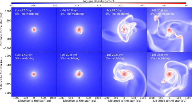
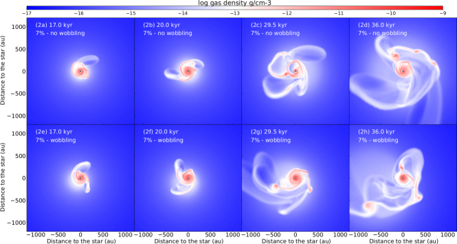
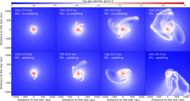
Figure 1: Density fields in the disc simulations with $\beta=5\%$ (top), $\beta=7\%$ (middle) and $\beta=9\%$ (bottom). The figures display the disc midplane gas density (in $\rm g\,\rm cm^{-3}$), for several characteristics time instances of the accretion disc evolution, without (upper panels) and with (lower panels) stellar wobbling.

3 Results

This section explores the evolution of the protostellar disc properties such as the disc radius and mass, for both simulations without and with the inclusion of the stellar motion of the central high-mass star. Similarly, we present how the intensity and duration of the accretion-driven bursts change when the star is allowed to move, for several initial conditions of the pre-stellar core.

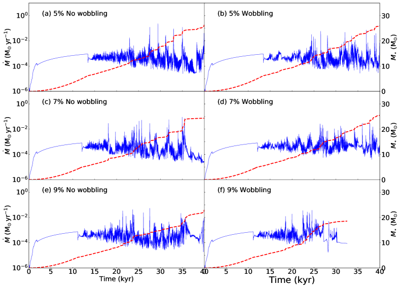
Figure 2: Accretion rate onto the protostar (in $\rm M_{\odot}\,\rm yr^{-1}$, solid blue line) and evolution of the mass of the young massive stellar objects (in $\rm M_{\odot}$) for our simulation models. The simulations are displayed for several $\beta$-ratio spanning from $5\%$ (top) to $9\%$ (bottom), without (left) and with (right) stellar motion.

3.1 Discs

3.1.1 Structure and evolution

In Fig. 1 we plot the midplane density field of the accretion discs (in $\rm cm^{-3}$) in our simulations with initial kinetic-to-gravitational energy $\beta=5\%$ (top series of panels), $\beta=7\%$ (middle series of panels) and $\beta=9\%$ (bottom series of panels). For each model, the discs are shown at several time instances as well as a later time, both without and with stellar inertia. In the figures, we only represent the inner ($\leq 1000\,\rm au$) part of the computational domain, for time instances that are older than the end of the free-fall gravitational collapse of the pre-stellar cloud and the onset of the disc formation. The accretion discs without stellar wobbling qualitatively evolve as described in the previous papers of this series, by undergoing efficient gravitational instabilities responsible for the formation of spiral arms and other rotating, self-gravitating substructures such as gaseous clumps and disc fragments (Meyer et al., 2018, 2019). Notable differences in the models with stellar inertia compared to the simulations with fixed star appear at times $\geq 25\,\rm kyr$.

The models without and with stellar inertia initially do not reveal differences, regardless of the $\beta$-ratio of the collapsing molecular cloud. This is visible in the left column of each panels showing the discs at time $17\,\rm kyr$. Their size increases as a function of the increasing $\beta$-ratio of the molecular cloud, because the timescale of the free-fall gravitational collapse is shorter for high $\beta$-ratio (see Fig. 2), hence at time $17\,\rm kyr$ the discs with $\beta=9\%$ are slightly older and more developed than that with $\beta=5\%$. The same is true at time $20.0\,\rm kyr$. Even tough the discs are qualitatively similar in terms of overall structure, differences begin to appear in their morphology, such as the number and the geometry of the growing spiral arms, see Fig. 1-1b,1f.

In our model with $\beta=5\%$, one can see at time $29.5\,\rm kyr$, that the disc with stellar wobbling has a rather compact structure wrapped by a large spiral arm (Fig. 1-1g), while the simulation without stellar wobbling has a more complex inner structure and exhibit signs of fragmentation both at its center and in a spiral arm extending to distance $>500\,\rm au$ from the protostar. The parent arm hosts a dense clump in the process of detaching from it, before migrating down to the protostar (Fig. 1-1c). At time $36.0\,\rm kyr$, both discs exhibit signs of active gravitational instability. The disc model without wobbling is more extended and has a (northern) very massive and large clump $\sim 1000\,\rm au$ from the protostar as well as a (southern) dense spiral arm (Fig. 1-1d), while the model with wobbling has a rounder and more compact structure in which enrolled spiral arms host a few clumps at distances $<500\,\rm au$ from the protostar (Fig. 1-1h). The discs are at different stages of internal reorganisation after it has experienced migrations of dense clumps onto the protostar, which generates an ejection of the clumps’ gaseous tails that reshuffle the whole disc structure (Meyer et al., 2018).

Hence, stellar wobbling moderately delays the fragmentation of the disc and reduces its entire size. The explanation is that when stellar wobbling is not considered, the accretion disc alone contains all the angular momentum of the star-disc system. Permitting the protostar to move (i) redistributes this angular momentum between the star and the disk with a net effect that the disk angular momentum decreases. Without stellar inertia, the discs turn to be of larger radius, and, therefore, their more extended spiral arms are more prone to fragment because disk fragmentation occurs predomenantly at large radii (Johnson & Gammie, 2003).

The above described effects of stellar wobbling in the disc evolution is equivalently found in the other simulation models with $\beta=7\%$ and $\beta=9\%$. The density field in the model with $\beta=7\%$ indeed displays similar features, with a disc with stellar inertia that fragments quicker than in the model with $\beta=5\%$, see Fig. 1-2c and Fig. 1-2g. Again, stellar inertia seems to make the circumstellar environment of the protostar more compact, with a smaller number of spiral arms. At time $36.0\,\rm kyr$ the disc with $\beta=7\%$ without stellar wobbling carries a larger number of clumps than the model with stellar wobbling, although they exhibit a similar qualitative level of fragmentation. Lastly, the model with $\beta=9\%$ slightly deviates from the simulations with $\beta\leq 7\%$. Because of its faster initial rotational velocity of the gas in the pre-stellar core, the development of gravitational instability in the disc takes more time than in the other models, see Fig. 1-3c and Fig. 1-3f. At later time ($36.0\,\rm kyr$), the effects of the indirect potential accounting for stellar inertia becomes so strong that the disc is strongly destroyed (see discussion on boundary effects in Section 4.1).

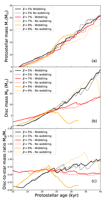
Figure 3: Protostellar mass (a), disc mass (b) and disc-to-star mass ratio (c) in our disc models with $\beta=5\%$ (black), $\beta=7\%$ (red) and $\beta=9\%$ (orange). Data for both models with (solid lines) and without (dashed-dotted lines) stellar wobbling are shown in the figure.

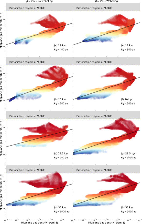
Figure 4: Evolution of the disc midplane in the density-temperature diagram for the model with $\beta=7\%$, without (left panels a-d) and with stellar inertia (right panels e-h), for different time from $17\,\rm kyr$ to $36\,\rm kyr$ after the beginning of the simulation. The color indicate the distance of each midplane gas element to the central protostar, normalised to the size of the disc at the considered time instance. The gray zone highlight the region with $T\geq 2000\,\rm K$ in which the gas is hotter than the molecular dissociation temperature. The black line is a fit to the entire dataset.

3.1.2 Protostellar accretion rate

Fig. 2 shows the accretion rate histories (thin solid blue line, in $\rm M_{\odot}\,\rm yr^{-1}$) and the stellar mass (thick dashed red line, in $\rm M_{\odot}$) of the young massive stellar objects forming in our simulations with kinetic-to-rotational energy radio $\beta=5\%$ (a,b), $7\%$ (c,d), $9\%$ (e,f). The left panels show the accretion rates of the models without wobbling, while the right panels plot the models with wobbling, respectively. In the panels, one can see the initial increase of the accretion rate during the free-fall collapse of the pre-stellar material, up to the time of the onset of the disc formation, at time $\approx 12\,\rm kyr$, when the accretion rate becomes variable because of azimuthal anisotropies in the accretion flow. At this time, the disc is small and of moderate size (Fig. 1-1a) and can be described to be in the so-called quiescent mode of accretion (Meyer et al., 2019).

At times $\approx 26\,\rm kyr$, the accretion rate history displays several strong peaks corresponding to the transport of disc material through the sink cell at rates $\geq 10^{-2}\,\rm M_{\odot}\,\rm yr^{-1}$. Those features characterise the burst mode of accretion in which the protostar enters when accreting dense segments of spiral arms and/or migrating gaseous clumps, and, this translates into luminous accretion-driven flares (Meyer et al., 2017, 2019). Star-disc systems in the burst mode are associated with large discs of complex internal structures (Fig. 2b). The rest of the modelled disc evolution is constituted of a succession of episodic accretion bursts interspersed by quiescent phases of accretion, which is characteristic of young stars growing and gaining mass within the burst mode of accretion (Meyer et al., 2019; Meyer et al., 2021). The evolution of the protostellar mass reflects this by displaying a series of step-like increases at the moment of the bursts (dotted red line of Fig. 2a), see also Meyer et al. (2018).

The accretion rate history of the model with $\beta=5\%$ including wobbling does not display strong qualitative differences in terms of accretion bursts compare to the models without stellar inertia, since the disc fragments (Fig. 1-1c,1g) and the protostar enters the burst mode of accretion at similar times ($\approx 24\,\rm Myr$). The same is true in our simulation with $\beta=7\%$. The accretion rate of the model with stellar wobbling and $\beta=9\%$ is much more erratic as a consequence of the dramatic distortion of the disc by the stellar wobbling, see Fig. 1-3h. Because the accretion bursts of the models with wobbling are of reduced magnitude, the mass evolution does not exhibit the large step-like increase of the mass evolution in the models with wobbling. In all our models, the magnitude and the number of the strongest accretion events is reduced when wobbling is included, see our Table 2.

3.1.3 Disc size, mass and disc-star mass ratio

Fig. 3 plots the properties of the simulated star-disc systems, such as the protostellar mass (top panel, in $\rm M_{\odot}$), the disc mass (middle panel, in $\rm M_{\odot}$) and the disc-to-star mass ratio (bottom panel). On each panel, the quantities are shown for all 6 models of Table 1 represented in the figures by a color coding, with thick solid lines (models without wobbling) and thin dashed lines (models with wobbling) for the simulations with $\beta=5\%$ (black), $\beta=7\%$ (red), $\beta=9\%$ (yellow). One can see that the protostellar mass histories are smoother in the simulations with wobbling than in those without, since, as discussed above, the onset of the gravitational instability happens sooner if no stellar inertia is included. However, in the models with $\beta=5\%$ and $\beta=7\%$, for the timescales of $40\,\rm kyr$ that we simulate, the final masses are similar, regardless of the physics taken into account in the simulation, as those simulations end with a final massive young protostellar object of $\approx 26\,\rm M_{\odot}$ and $\approx 25\,\rm M_{\odot}$, respectively. Inversely, for high $\beta$-ratio of $9\%$, it reveals a notable difference of a few solar mass between the stellar mass calculated without and with wobbling at times $\approx 32.5\,\rm kyr$, as a direct consequence of gravitational instability boundary effects influencing the disc evolution in this fast-spinning system.

The middle panel of the figure (Fig. 3b) shows the evolution of the disc mass, calculated by integrating the gas density in a cylinder of dimensions $2000\,\rm au$ and height $500\,\rm au$ as in Klassen et al. (2016); Meyer et al. (2018). The disc mass evolution $M_{\rm d}$ (in $M_{\odot}$) is marked by abrupt decreases corresponding to the time instances when dense gaseous clumps disappear into the central sink cell of radius $r_{\rm in}=20\,\rm au$, also provoking step-like increase of the protostellar mass history (Fig. 3a). Indeed, when a clump is accreted and the mass and disc evolution have opposite variability, the first gains the amount of mass the latter loses. Note that the disc masses do not sensibly change whether wobbling is included or not, at least for the time that we simulate ($40\,\rm kyr$), except for the model with $\beta=9\%$ that is affected by strong wobbling-related boundary issues (Section 4.2). The bottom panel shows the evolution of the disc-to-star mass ratio $M_{\rm d}/M_{\star}$ (Fig. 3c) which remains $\geq 0.5$ once the accretion discs form (Meyer et al., 2021), throughout all the simulations, except for the model with $\beta=9\%$ and unfixed star, which deviates from this trend starting from time $\approx 25\,\rm kyr$ when the effects of the stellar wobbling are so strong that they induce a stretching of the circumstellar disc (see Fig. 1-3c, Fig. 1-3h and also Section 4.1).

Table 2: Table displaying the main properties of the accretion bursts in our simulations series with $\beta=5\%$$-$$9\%$. $N_{\mathrm{bst}}$ is the number of bursts undergone by the protostars at a given magnitude class. $L_{\mathrm{max}}/L_{\mathrm{min}}/L_{\mathrm{mean}}$ stands for the maximum, minimum, and mean burst luminosities. Equivalently, $\dot{M}_{\mathrm{max}}/\dot{M}_{\mathrm{min}}/\dot{M}_{\mathrm{mean}}$ correspond to the accretion rates onto the protostar, and $t_{\mathrm{bst}}^{\mathrm{max}}$/$t_{\mathrm{bst}}^{\mathrm{min}}$/$t_{\mathrm{bst}}^{\mathrm{mean}}$ relate to the accretion burst duration. $t_{\mathrm{bst}}^{\mathrm{tot}}$ is the total time a massive young stellar object spends bursting via a given burst magnitude class.

Model	$N_{\mathrm{bst}}$	$L_{\mathrm{max}}/L_{\mathrm{min}}/L_{\mathrm{mean}}$ ($10^{5}\,\rm L_{\odot}$)	$\dot{M}_{\mathrm{max}}/\dot{M}_{\mathrm{min}}/\dot{M}_{\mathrm{mean}}$ ($\rm M_{\odot}\,\rm yr^{-1}$)	$t_{\mathrm{bst}}^{\mathrm{max}}$/$t_{\mathrm{bst}}^{\mathrm{min}}$/$t_{\mathrm{bst}}^{\mathrm{mean}}$ $\rm(yr)$	$t_{\mathrm{bst}}^{\mathrm{tot}}$ $\rm(yr)$
1-mag cutoff
Run-256-100$\rm M_{\odot}$-5$\%$-wio	6	19.89 / 0.464 / 5.40	0.0397 / 0.0073 / 0.0170	15 / 4 / 9	51
Run-256-100$\rm M_{\odot}$-5$\%$-wi	10	3.65 / 0.494 / 2.05	0.0211 / 0.0065 / 0.0103	35 / 6 / 14	135
Run-256-100$\rm M_{\odot}$-7$\%$-wio	13	2.24 / 0.079 / 0.88	0.0224 / 0.0016 / 0.0087	33 / 8 / 14	182
Run-256-100$\rm M_{\odot}$-7$\%$-wi	14	6.2 / 0.067 / 1.79	0.0211 / 0.0015 / 0.0110	36 / 5 / 13	175
Run-256-100$\rm M_{\odot}$-9$\%$-wio	16	2.25 / 0.051 / 0.66	0.0239 / 0.0011 / 0.0088	74 / 5 / 19	304
Run-256-100$\rm M_{\odot}$-9$\%$-wi	11	1.06 / 0.052 / 0.32	0.0231 / 0.0011 / 0.0077	23 / 7 / 12	134
Total all models	70				163
2-mag cutoff
Run-256-100$\rm M_{\odot}$-5$\%$-wio	3	4.20 / 2.136 / 3.17	0.0295 / 0.0220 / 0.0265	14 / 5 / 10	30
Run-256-100$\rm M_{\odot}$-5$\%$-wi	7	17.03 / 1.338 / 7.02	0.0585 / 0.0245 / 0.0366	18 / 4 / 10	70
Run-256-100$\rm M_{\odot}$-7$\%$-wio	3	3.01 / 2.014 / 2.40	0.0523 / 0.0286 / 0.0414	9 / 4 / 8	23
Run-256-100$\rm M_{\odot}$-7$\%$-wi	3	9.13 / 1.248 / 5.84	0.0309 / 0.0262 / 0.0285	42 / 4 / 25	74
Run-256-100$\rm M_{\odot}$-9$\%$-wio	5	2.99 / 0.207 / 1.57	0.0531 / 0.0041 / 0.0308	11 / 5 / 8	41
Run-256-100$\rm M_{\odot}$-9$\%$-wi	4	2.29 / 0.243 / 1.09	0.0372 / 0.0049 / 0.0261	14 / 5 / 10	40
Total all models	25				46
3-mag cutoff
Run-256-100$\rm M_{\odot}$-5$\%$-wio	3	34.28 / 8.977 / 21.32	0.1207 / 0.0910 / 0.1083	12 / 3 / 6	18
Run-256-100$\rm M_{\odot}$-5$\%$-wi	1	21.66 / 21.661 / 21.66	0.0723 / 0.0723 / 0.0723	3 / 3 / 3	3
Run-256-100$\rm M_{\odot}$-7$\%$-wio	4	22.17 / 1.344 / 11.59	0.0888 / 0.0286 / 0.0610	15/4/7	28
Run-256-100$\rm M_{\odot}$-7$\%$-wi	-	-	-	-	-
Run-256-100$\rm M_{\odot}$-9$\%$-wio	-	-	-	-	-
Run-256-100$\rm M_{\odot}$-9$\%$-wi	2	0.83 / 0.608 / 0.72	0.0188 / 0.0122 / 0.0155	13 / 8 / 11	22
Total all models	10				18
4-mag cutoff
Run-256-100$\rm M_{\odot}$-5$\%$-wio	1	23.80 / 23.801 / 23.80	0.2313 / 0.2313 / 0.2313	2 / 2 / 2	2
Run-256-100$\rm M_{\odot}$-5$\%$-wi	-	-	-	-	-
Run-256-100$\rm M_{\odot}$-7$\%$-wio	-	-	-	-	-
Run-256-100$\rm M_{\odot}$-7$\%$-wi	-	-	-	-	-
Run-256-100$\rm M_{\odot}$-9$\%$-wio	-	-	-	-	-
Run-256-100$\rm M_{\odot}$-9$\%$-wi	-	-	-	-	-
Total all models	1				2

Figure 5: Distribution of the accretion-driven bursts in our series of simulation models in the burst duration-burst peak luminosity (a) and burst duration-burst accreted mass per burst (b) planes. The burst duration is in $\rm yr$, the burst peak luminosity in $\rm L_{\odot}$ and the accreted mass per burst in $\rm M_{\odot}$, respectively. The burst are displayed for both the disc modelled without (red squares) and with (yellow triangles) stellar inertia. The figure indicates the burst modelled in the previous papers of this series as black circles (Meyer et al., 2021). The size of the symbols scale with the magnitude of the accretion-driven burst, from the smallest (1-mag bursts), to the largest (4-mag) bursts. Note that the single 4-mag burst of this high-resolution series of models is marked in magenta. Note that all except one single 4-mag bursts belong to the data in Meyer et al. (2021).

3.1.4 Disc thermodynamics

In Fig. 4 the time-evolution of the disc midplane temperature is displayed as a function of the midplane gas density for the models with $\beta=7\%$ without (left panels) and with wobbling (right panels), for times spanning from $17\,\rm kyr$ to $36\,\rm kyr$. Color-coding shows the distance to the central protostar $r/R_{\rm disc}$ for each point in the figure, normalised to the disc size, with $R_{\rm disc}$ the maximum disc radius at a considered time, which we measure by tracking the region at which the infalling material lands onto the disc, using the azimuthaly-averaged midplane velocity profiles. The black line represents a fit to the whole dataset and the upper grayed region ($T\geq 2000\,\rm K$) highlights the temperature above which molecular hydrogen dissociates. The diagonal branch along which both density and temperature increase as we go from larger to smaller distances, as typically protoplanetary discs do. The outer diluted and cold disc region (blue points) exhibit less horizontal deviation from the diagonal black line than the dense, hot inner part (red points), especially at after the beginning of the disc formation (Fig. 1-2a, Fig. 1-2e). There is a turn-over and a horizontal branch corresponding to the very inner disc regions that is warmer than the diagonal region, although density can vary in a wide range. Only in this region the gas temperature exceeds the molecular hydrogen dissociation threshold ($T\geq 2000\,\rm K$).

At later times, when the disc has begun to fragment, the horizontal deviations in the inner region is more pronounced as a result of the growth of the disc and scatter over a wider density range. The disc structure adopts a more complex morphology provoking additional branches in the high temperature part of the diagram, accounting for the many spiral arms forming by gravitational instability and enrolling around the sink cell (Fig. 4b). At time $29.5\,\rm kyr$ the disc strongly fragments (Fig. 4c). The gaseous clumps extend as a horizontal high temperature branch $\sim 500\,\rm au$ from the star. This upper region further evolves as the disc keeps on fragmenting, and more clumps form within the extended spiral arms, which translates into a scattering of the low-temperature region (blue dots of Fig. 4d).

The disc model with wobbling included is qualitatively similar to its fixed-star counterpart at time $17\,\rm kyr$ (Fig. 4a,e) in both structure and thermodynamical properties, except regarding the disc without stellar inertia is $25\%$ larger since its radius reaches $400\,\rm au$ at that time whereas the other disc model extends up to $300\,\rm au$ only. At time $20\,\rm kyr$ the disc with wobbling does not exhibit the group of high temperature and high density point scattering close to the dissociation temperature regime (Fig. 4b,f), because the disc model with fixed protostar fragments more violently. The absence of early clumps in the model with wobbling results in a distribution of the disc midplane gas along the diagonal with much less scattering with respect to the black line (Fig. 4c,g), whereas the inner disc region is hotter and exceed the molecular hydrogen dissociation temperature. The disc, having fragments located in the inner region ($\leq 200\,\rm au$), is on the road to multiplicity (Meyer et al., 2018). Indeed, disc gas exceeding $2000\,\rm K$ implies second Larson collapse (Larson, 1969, 1972) and formation of a protostar, which is not resolved in our simulations, and, therefore, multiplicity can only be inferred from this diagram. At this time, the disc without stellar inertia is more compact than that with wobbling. Finally, at time $36\,\rm kyr$ both discs are violently fragmenting and have the same overall size of $\approx 1000\,\rm au$.

3.2 Bursts

We perform an analysis of the variability in the accretion rate histories onto the young massive stellar objects. The stellar mass and accretion rate measured in the radiation-hydrodynamics simulations are turned into a lightcurve via the estimate of the protostellar radius, interpolated from the evolutionary tracks of Hosokawa & Omukai (2009). Then, the total luminosity of the central massive young stellar objects is calculated for each model as $L_{\rm tot}=L_{\star}+L_{\rm acc}$, with $L_{\star}=L_{\star}(M_{\star},\dot{M})$ the photospheric luminosity from Hosokawa & Omukai (2009) and $L_{\rm acc}=fGM_{\star}\dot{M}/R_{\star}$ the accretion luminosity, where $G$ is the universal gravitational constant, $f=3/4$ a factor accounting for the effective mass accreted onto the stellar surface, the rest being released into the a protostellar jet. Hence, the variability of the accretion rate reflects onto evolution of the total luminosity, see fig. 3. of Meyer et al. (2021). For each model, the lightcurves $L_{\rm tot}(t)$ are post-processed with the signal analysis method developed in Vorobyov et al. (2018), which filters out the accretion bursts from a synthetic quiescent background luminosity $L_{\rm bg}$. During each burst, the luminosity peak is compared to $L_{\rm bg}$ and the ongoing flare is classified as an $i$-magnitude ($i$-mag) burst, with $i$ such that $L_{\rm tot}\geq 2.5^{i}L_{\rm bg}$. The method ensures that small variabilities of magnitude $\leq i=1$, either from the vicinity of the sink cell or from the secular evolution of $L_{\rm bg}$, are not confused with true bursts (Elbakyan et al., 2019). The results for the bursts analysis are summarised in Table 2.

Models for the circumstellar medium of young massive stars show that the total number of bursts measured in the simulations decreases as their magnitude increases. In other words, there are more 1- and 2-mag bursts than 3- and 4-mag flares, and a similar tendency is found for the total time spent in the burst mode as a function of the burst magnitude, e.g. we count 70 1-mag bursts in total and only a single 4-mag burst in our entire series of simulations. This trend of declining burst activity of young massive stars is not modified when including wobbling in the simulations. The effect of disc wobbling on the burst properties can be summarised as follows. The number of 1-mag bursts varies at most by up to a factor of $\approx 2$ when allowing the protostar to move. The number of 2-mag bursts only differs by 1$-$2 bursts in the models with and without wobbling. Major differences appear with the 4-mag bursts, i.e. only a model without wobbling is able to produce such event, at least for the time interval that we simulate.

Additionally, higher-magnitude bursts are also much less common than their 1-mag counterparts. Only the model with $\beta=5\%$ without wobbling exhibit a short 4-mag burst of duration $2\,\rm yr$, suggesting that the realistic discs with stellar inertia do not undergo such mechanisms, at least during the early $\approx 40\,\rm kyr$ of their evolution. Higher-resolution simulations are required to further investigate the question of FU-Orionis-like bursts in massive star formation. The average luminosity of the 3-mag bursts is similar regardless of the physics included into the models, however, the models without wobbling can accreted slightly more mass per bursts.

Table 3: Proportion (in $\%$) of mass gain at the end of our simulation, as a function of the flare magnitude during the burst phase of accretion. The intensity of each individual burst is defined as in Meyer et al. (2019).

${\rm{Models}}$	$\beta$-ratio	${\rm{Inertia}}$	$\rm L_{\rm tot}\sim\,\rm L_{\rm bg}$	$1$$-$$\rm mag$	$2$$-$$\rm mag$	$3$$-$$\rm mag$	$4$$-$$\rm mag$
Run-256-100$\rm M_{\odot}$-5$\%$-wio	$5\,\%$	no	81.67	11.86	5.07	1.37	0.03
Run-256-100$\rm M_{\odot}$-7$\%$-wio	$7\,\%$	no	81.76	12.59	5.62	0.03	0.0
Run-256-100$\rm M_{\odot}$-9$\%$-wio	$9\,\%$	no	88.10	9.02	2.88	0.0	0.0
Mean	-	-	83.84	11.16	4.53	0.46	0.01
Run-256-100$\rm M_{\odot}$-5$\%$-wi	$5\,\%$	yes	77.54	11.17	4.61	6.65	0.0
Run-256-100$\rm M_{\odot}$-7$\%$-wi	$7\,\%$	yes	73.26	16.62	10.12	0.0	0.0
Run-256-100$\rm M_{\odot}$-9$\%$-wi	$9\,\%$	yes	84.20	10.98	4.18	0.64	0.0
Mean	-	-	78.34	12.92	6.31	2.43	0.0

In Fig. 5 the burst duration is plotted as a function of the maximum luminosity of each accretion-driven bursts (panel a), and as a function of the mass accreted throughout the burst (panel b). On the panels, the circles represent the data reported in the previous papers of this series which were computed at a lower spatial resolution (Meyer et al., 2021), and the circle size scales with the burst magnitude. The data for the current study are plotted as red squares (models without wobbling) and yellow triangles (models with wobbling). The bursts of lower magnitude (1-mag) are located in the $\leq 5\times 10^{5}\,\rm L_{\odot}$ region of the plot, regardless of their duration, spanning from a few $1\,\rm yr$ to $\approx 10^{2}\,\rm yr$ (Fig. 5a). The high magnitude bursts (3- and 4-mag bursts) are found in the rather short duration ($\leq 20\,\rm yr$) and higher luminosity ($>10^{5}\,\rm L_{\odot}$) region of the figure, although a few bursts without wobbling do not follow this rule and are located in the long duration region of the figure. This is in accordance with simulations of lower spatial resolution (empty circles), however, the burst distribution in our simulations do not extend to the same upper limit in terms of the peak luminosity because of the absence of 4-mag bursts in our sample. The bursts are shorter and dimmer compared to a $128\times 11\times 128$ simulation. Importantly, the duration of the high-magnitude bursts in the model with wobbling is of slightly lower duration than those found in the simulation with fixed star. In the burst duration-accreted mass plane (Fig. 5b) we see that lower-magnitude bursts distribute along diagonals which indicate that the accreted mass scales linearly with the burst duration. Once again, as detailed in Meyer et al. (2021), some of the most mass-accreting bursts are amongst the faintest, since the total luminosity $L_{\rm tot}$ is dominated by the accretion luminosity $L_{\rm acc}\propto 1/R_{\star}$, with $R_{\star}$ increasing during the burst phase, when the protostar experiences excursions to the cold part of the Herzsprung-Russell diagram (Meyer et al., 2019).

In Table 3 we report the proportion of final mass accreted by our protostars during the quiescent and the burst phases, separated, for the latter, by the magnitude of the accretion-driven bursts. The mean proportion of final mass accreted during the burst phase of accretion amounts $\approx 17\%$ for the models without wobbling and $\approx 22\%$ when stellar inertia is included, respectively. Similarly, the average mass accreted during 1-mag bursts is $\approx 11$$-$$12\%$ with or without stellar wobbling, with a slight increase as a function of $\beta$-ratio. Differences mostly happen for the 2-mag bursts, with $\approx 4.5\%$ and $\approx 6.3\%$ of the total accreted mass with and without wobbling, respectively. Similarly, the protostars modelled with stellar inertia gain $\approx 2.4\%$ of their mass experiencing 3-mag bursts. None of the models accrete mass via 4-mag bursts, since they are absent from the present simulations, except in the model without wobbling and $\beta=5\%$ which produced a single occurrence of such a burst. In Meyer et al. (2019); Meyer et al. (2021), we concluded that massive stars gain up to half of their zero-age-main-sequence mass by mass accretion in the burst mode, on the basis of models run up to $\sim 70\,\rm kyr$. It is the later phase of the disc evolution that the strongest bursts appeared, while we stop our models sooner in the present study, because of the enormous computational costs of our higher-resolution calculations.

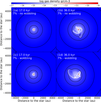
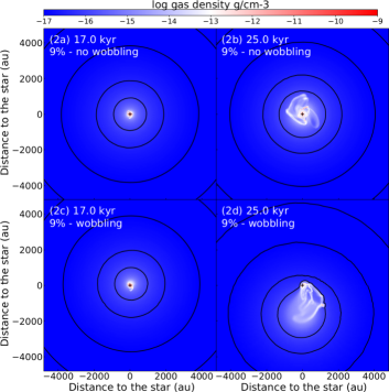
Figure 6: Disc midplane with $\beta=7\%$ (upper series of panels) and $\beta=9\%$ (lower series of panels), and, each of them displaying both models with (top) and without (bottom) wobbling. The figures show the disc midplane gas density, (in $\rm g\,\rm cm^{-3}$) for several selected characteristics time instances of the accretion disc evolution, and with solid black number density isocontours highlighting the effects of the stellar inertia onto the mass distribution in the computational domain.

4 Discussion

This section reminds the reader the limitations of our simulation setup and discuss the observability of the accretion disc models if observed by means of the alma interferometer.

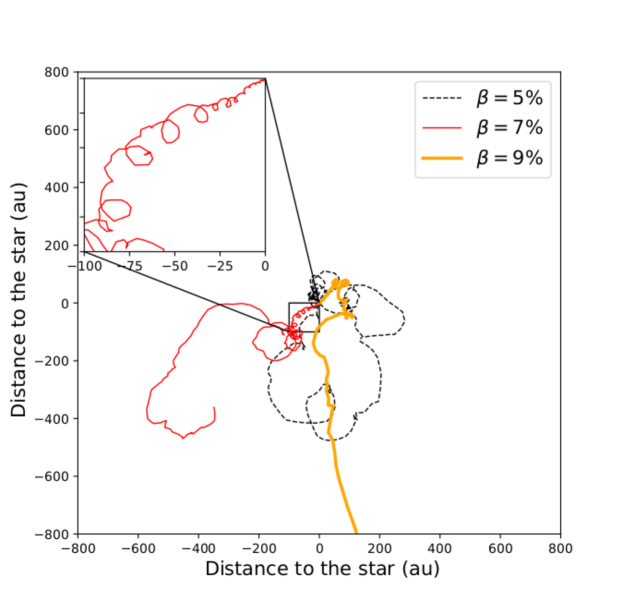
Figure 7: Time evolution of the position of the center of mass of the accretion discs modelled with stellar inertia (in $\rm au$), for our simulation with $\beta=5\%$ (black dashed line), $\beta=7\%$ (red thin solid line) and $\beta=9\%$ (orange thick solid line). Inset plot zooms on the wobbled motion induced by the stellar inertia.

4.1 Caveats

Most of the limitations in the numerical method utilised in this study have been presented in the parameter study (Meyer et al., 2021), particularly regarding the absence of magnetic fields, non-ideal magneto-hydrodynamics and photoionisation that mostly affect the bipolar jet filled with hot gas. While the magnetic feedback should be improved in future studies, not taking into account the protostellar ionization is acceptable since we concentrate onto the disc structure and its properties. Nevertheless, disc evaporation and disc wind are neglected in the simulations. This work explores the stellar motion induced by the disc in the fashion of Michael & Durisen (2010a); Regály & Vorobyov (2017) with moderate-resolution $256\times 41\times 256$ simulations, which is a major improvement relative to the models presented in Meyer et al. (2018) and Meyer et al. (2019) since our work is based on both high-resolution models performed with stellar inertia. Nevertheless, the midplane symmetry that we impose to our calculations intrinsically neglects any vertical motion of the massive protostar, although low-resolution tests suggested that this effect is not important (Meyer et al., 2018). In future studies we will consider higher-resolution models like those presented in Oliva & Kuiper (2020). The increased resolution of our simulations imposed to move the size of the inner radius of the sink cell $r_{\rm in}$ to $20\,\rm au$ instead of $10\,\rm au$ in Meyer et al. (2018, 2019). As the time-step restrictions are principally governed by the size of the innermost cell of the radial logarithmically expanding mesh, we had to keep the calculations affordable from the point of view of the computational costs.

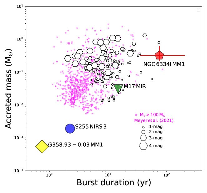
Figure 8: Comparison of our modelled bursts with the properties of observed bursts in the burst duration-accreted-mass diagram. The white hexagons are the burst from the simulated discs presented in this study, the coloured symbols stand for the burst observed so far from young high-mass stellar objects. The magenta stars represent the burst from the models with an initial molecular core model $M_{\rm c}\geq 100\,\rm M_{\odot}$ in Meyer et al. (2021).

As observed in Michael & Durisen (2010a) and (Regály & Vorobyov, 2017) in the context of accretion discs of low-mass stars, stellar inertia delays the development of gravitational instabilities in the disc and modifies its overall appearance, in particular the spatial morphology of the structures growing in it. While the consideration of stellar inertia adds realism of the simulated models, it also introduces an additional boundary effect related to the displacement of the disc in the computational domain that mimics the stellar displacement in the non-inertial frame of reference. This particularly takes place when the mass of the disc is comparable to that of the protostar $M_{\rm d}/M_{\star}\approx 1$, as it is the case in the formation of our massive stars (Fig. 3b, see also our model with $\beta=7\%$ in Fig. 1-3h). However, the timescales over which high-mass stars operate ($\sim\rm kyr$) is much shorter than that of their lower mass counterparts ($\rm Myr$), and, therefore, the boundary effects are somehow less pronounced in our models except in the simulation with high $\beta$-ratio. An updated version of the code should handle moving boundaries and/or replenishing the void caused by means of the displacement of the density field by infalling pre-stellar core material that is initially out of the computational domain at radii $r\geq R_{\rm max}$.

4.2 Effect of wobbling on disc structure

Fig. 6 shows a zoomed-out view of the midplane density field in ($\rm g\,\rm cm^{-3}$) of the computational domain in our simulations with $\beta=7\%$ (top panels) and $\beta=9\%$ (bottom panels) for several selected time instances of the system evolution. The figures cover a region of $5000\times 5000\,\rm au$ including both the accretion disc in the inner $\leq 1000\,\rm au$ and the still-collapsing pre-stellar core. Density isocontours as solid black lines highlight the structure of the density field of the molecular envelope and the disc. At $17\,\rm kyr$, the midplane density in the collapsing envelope is axisymmetric as were the initial conditions for the pre-stellar core (Eq. 1), in both simulation with and without wobbling, see also Fig. 6 1a-1c (top). Almost at the end of the simulation (at time $\geq 36\,\rm kyr$) the deviation from the axisymmetry of the initial density structure is pronounced in the case with stellar inertia (Fig. 6 1d), as the stellar motion affects not only the accretion disc located in the inner region of the computational domain, but also the whole envelope. For fast initial rotation of the pre-stellar core ($\beta\geq 9\%$), the deviations from axisymmetry are magnified and happen quicker, at time $25\,\rm kyr$, see Fig. 6 2d (bottom). The catastrophic effects of stellar wobbling on the envelope and disc evolution are caused by the fact that the acceleration caused by the non-inertial frame of reference shifts the material in the entire computational domain. As a result, a distortion in the gas density near the outer fixed boundary develops, which gradually feeds back and modifies through gravity the entire evolution of the inner structure.

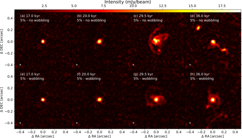
Figure 9: Synthetic emission maps of the models with $\beta=5\%$, without (top panels) and with (bottom panels) stellar inertia, as seen by the ALMA interferometer in its antenna configuration 10. The disc are shown at the same characteristic times as for the upper series panels in Fig. 1. The distance to the source is assumed to be $1\,\rm kpc$.

We display the evolution of the position of the barycenter of the star-disc-envelope system in Fig. 7. The center of mass is calculated as,

$$x_{\mathrm{bar}}(t)=\frac{1}{M}\sum_{\rm ijk}x_{\rm ijk}\rho_{\rm ijk}dV_{\rm ijk},$$ (24)

$$y_{\mathrm{bar}}(t)=\frac{1}{M}\sum_{\rm ijk}y_{\rm ijk}\rho_{\rm ijk}dV_{\rm ijk},$$ (25)

and,

$$z_{\mathrm{bar}}(t)=\frac{1}{M}\sum_{\rm ijk}z_{\rm ijk}\rho_{\rm ijk}dV_{\rm ijk},$$ (26)

where,

$$x_{\rm ijk}=r_{\rm ijk}\cos(\phi_{\rm ijk})\sin(\theta_{\rm ijk})$$ (27)

$$y_{\rm ijk}=r_{\rm ijk}\cos(\phi_{\rm ijk})\sin(\theta_{\rm ijk})$$ (28)

and,

$$z_{\rm ijk}=r_{\rm ijk}\cos(\theta_{\rm ijk})$$ (29)

are the Cartesian coordinates of a disc volume element $ijk$, respectively. The midplane symmetry of the computational domain imposes $z_{\rm bar}=0$ and the whole mass $M$ included into it reads,

$$M=\iiint\rho dV=\sum_{\rm ijk}\rho_{\rm ijk}dV_{\rm ijk},$$ (30)

where $dV_{\rm ijk}$ is the volume element of the grid zone $ijk$ in the computational domain, with $1\leq i\leq 256$, $1\leq j\leq 41$ and $1\leq k\leq 256$. The barycenter exhibits large excursions from the origin of the computational domain ($x=0,y=0$, $z=0$) as well as smaller-scale periodic deviations from the path of the excursions. The large-scale motion is a direct consequence of the non-axisymmetric shape adopted by the infalling molecular material of the envelope and, as the $\beta$-ratio of the model increases, the excursions of the star away from the origin are more important (see yellow line of Fig. 7). The small amplitude displacement of the barycenter is caused by of the development of substructures in the disc, such as dense spiral arms and gaseous clumps, which are of much milder effects.

Figure 10: Cuts through the synthetic emission maps of our accretion disc model with $\beta=5\%$ (in $\rm mJy\,\rm beam^{-1}$) for the inner disc region. Each panel show the surface brightness without (solid red line) and with stellar inertia (dashed blue line). The horizontal lines of panels display the data for a same time instance, and each column correspond to a different cut through the emission maps, measured clock-wise, and characterised by the angle $\phi$ of the cut with respect to its vertical north-south direction.

4.3 Comparison with monitored bursts

Fig. 8 compares our modelled bursts with the properties of observed flares, in the burst duration-accreted mass diagram. The white hexagons are the burst measures from the lightcurves calculated on the basis of the accretion rate histories of our simulated protostars and the coloured symbols stand for real bursts of high-mass stars. The red pentagon represents the burst of NGC 6334I MM1, which duration has been constrained to $t_{\rm bst}\approx 40$$-$$130\,\rm yr$ (Hunter et al., 2021) and the correspondingly accreted mass estimated to $M_{\rm bst}\approx 0.1$$-$$0.3\,\rm M_{\odot}$ (Hunter et al., 2021; Elbakyan et al., 2021). Similarly, the yellow diamond marks the burst of G358.93-0.003 MM1, which properties are $t_{\rm bst}\approx 0.75\,\rm yr$ and $M_{\rm bst}\approx 0.566\,\rm M_{\rm J}$ (Stecklum et al., 2021; Elbakyan et al., 2021). The blue circle and the green triangle stand for the bursts monitored from the young massive stellar object S255 NIRS 3 ($t_{\rm bst}\approx 2.25\,\rm yr$, $M_{\rm bst}\approx 2\,\rm M_{\rm J}$), see Caratti o Garatti et al. (2017); Elbakyan et al. (2021), and that of the recently-discovered outbursts of M17 MIR ($t_{\rm bst}\approx 15\,\rm yr$, $M_{\rm bst}\approx 31.43\,\rm M_{\rm J}$), see Chen et al. (2021); Elbakyan et al. (2021) and references therein.

The bursts observed from S255 NIRS 3 and G358.93-0.003 MM1 have a smaller amount of accreted mass compared to that found in our simulations, while their duration is consistent with our data, although G358.93-0.003 MM1 is shorter by an order of magnitude than the shortest burst duration measured from our models. This, however, can be explained by our too big inner sink cell radii. The use of a smaller sink would give the infalling gaseous clumps more time to lose their outer envelope via tidal stripping when migrating closer to the star, as studied in the so-called tidal downsizing model (Nayakshin, 2015a, b; Nayakshin & Fletcher, 2015; Nayakshin, 2016). Consequently, the actual mass of the clump would become smaller as it approaches the star and only the core would survive. The accreted mass value observed for the burst of NGC 6334I MM1 is consistent with our modelled burst. This burst being classified as a 3-mag burst in the parlance of our simulations for the burst mode of accretion in massive star formation (Hunter et al., 2021), however, our models predict that such burst should be of slightly shorter duration. Such discrepancy could be explained by the fact that the initial properties of the molecular cloud in which NGC 6334I MM1 forms might probably be different than that assumed in our simulations. The outburst of M17 MIR shows much more consistencies with our predictions, both in terms of duration and accreted mass (green triangle). The magenta stars of Fig. 8 are the bursts from the models with initial molecular cores $M_{\rm c}\geq 100\,\rm M_{\odot}$ (Meyer et al., 2021), which have smaller accreted mass than the bursts of the present study which all assume $M_{\rm c}=100\,\rm M_{\odot}$. We speculate that the initial core of M17 MIR is perhaps of smaller mass than that responsible for the formation of the other protostars, i.e. S255 NIRS 3 and G358.93-0.003 MM1. Future studies tailored to particular bursts should take this into account.

Last, let’s also underline that the observational measures of the burst properties are affected by a certain number of uncertainties. The burst properties are principally derived by measuring the variability in brightness temperature of the object, assumed to be equal to that of the dust temperature, from which the luminosity is calculated. This relies on geometrical effects potentially scattering radiation out of the observer’s light-of-sight, and therefore decreasing the monitored brightness temperature and radiation intensity (Hunter et al., 2017). Additionally, absorption effects are at work, reducing the observed dust continuum flux and drastically reducing the observed accretion luminosity from which the accreted mass is derived (Johnston et al., 2013). Consequently, the real data in the burst duration-accreted mass diagram, represented by coloured symbols in Fig. 8 are not firm numbers, but high uncertainties estimates. Future observational work on the finer characterisation of burst properties would be highly desirable.

4.4 Emission maps and observability

We repeat the exercise of calculating predictive alma images for the simulated discs as done in Meyer et al. (2019), see also MacFarlane et al. (2019a, b); Skliarevskii et al. (2021). The dust density field calculated with the pluto code, taking into account the information about dust-sublimated regions, is imported into the radiative transfert code radmc-3d (Dullemond, 2012) for the characteristic simulation snapshots of the model with $\beta=5\%$ in Fig. 1. It first calculates the dust temperature by Monte-Carlo simulation using the method of Bjorkman & Wood (2001) before ray-tracing $10^{8}$ photons packages from the stellar surface to the disc. Then, it performs radiative transfer calculations against dust opacity assuming that the dust in the disc is the silicate mixture of Laor & Draine (1993). The source of photons is considered to be a black body of effective temperature $T_{\rm eff}$ determined for each disc snapshots using the stellar evolutionary tracks of Hosokawa et al. (2010).

Synthetic images of the disc are produced for a field of view covering a radius of $1000\,\rm au$ around the central protostar and made of $2000\times 2000$ grid zones onto which the emissivity is projected. Images are calculated at $249.827\,\rm Ghz$ ($1.2\,\rm mm$) with a channelwidth of $50.0\,\rm Mhz$ which corresponds to the alma band 6, assuming no inclination angle for the accretion disc with respect to the plane of the sky. Last, the simulated emission maps are treated with the Common Astronomy Software Applications casa (McMullin et al., 2007). We obtain simulated interferometric images which can be directly compared to the data acquired by the alma facility. The antennae are assumed to be in the most extended, long-baseline spatial configuration C43-10 using 43 $12\,\rm m$ antennae permitting to reach a maximal spatial resolution of $0.015^{"}$. The distance to the source is assumed to be $1\,\rm kpc$. We refer the reader interested in further details on our method for simulating the synthetic images (Meyer et al., 2019).

Fig. 9 plots the $1.2\,\rm mm$ synthetic alma emission maps of the disc model with the rotation-to-gravitational ratio $\beta=5\%$, without (top panels) and with stellar inertia (bottom panels), for the characteristic time instances of the disc evolution presented in Fig. 1-1. The images at time $17\,\rm kyr$ consist of a bright circle representing the nascent disc, right after the end of the free-fall gravitational collapse of the cloud material (Fig. 9a). This remains unchanged up to time $20\,\rm kyr$, since the star has not yet entered the burst mode and keeps on gaining mass by quiescent accretion from a stable and unfragmented disc (Fig. 1-1b). The model with stellar inertia does not exhibit identifiable substructures either at a similar time of evolution (Fig. 1-1e-f). At time $29.5\,\rm kyr$ the circumstellar medium of the massive protostar is made of a bright central stellar region, accompanied by a visible infalling gaseous clump in the close stellar surroundings. The entire structure is surrounded by a large-scale spiral arm wrapped around the inner disc (Fig. 9c). Note that the very extension of the spiral arm is not visible, hence, the observed disc does not fully reflect the entire size and composition of the whole object, see midplane density field in Fig. 1-1c. Fragmentation further modifies the disc millimeter appearance which takes the typical morphology of a massive double protosystem, see image Fig. 9d.

The simulation model including stellar inertia displays a typical two-armed structure at $29.5\,\rm kyr$ (Fig. 9g) and a more complex pattern at the end of the simulation, including an inner enrolled spiral arms, gaseous clumps and more extended arms with fainter clumps in the southern region (Fig. 9h). The spiral arms reveal a certain level of granulosity arising from the interferometric measures, not originating from the disc structure itself (Fig. 9c), and this can be misinterpreted as additional disc fragments as of the same brightness as the faintest gaseous clumps. These models take their importance in the context of the recently observed bursting young massive protostars and their circumstellar environments (Johnston et al., 2015; Chen et al., 2016; Ilee et al., 2016; Forgan et al., 2016; Maud et al., 2017; Chen et al., 2017; Maud et al., 2018; Ahmadi et al., 2018; Ilee et al., 2018; Maud et al., 2018; Sanna et al., 2019; Motogi et al., 2019; Maud et al., 2019; Liu et al., 2020; Sanna et al., 2021; Suri et al., 2021; Humphries et al., 2021; Vorster et al., 2021; Williams et al., 2022; McCarthy et al., 2022).

Fig. 10 displays cross-sections through the simulated images of the disc models without (solid red line) and with (dashed blue line) stellar wobbling plotted in Fig. 9 for several angles $\phi=0\mathrm{\SIUnitSymbolDegree}$, $45\mathrm{\SIUnitSymbolDegree}$, $90\mathrm{\SIUnitSymbolDegree}$ and $\phi=120\mathrm{\SIUnitSymbolDegree}$ with respect to the north-south axis. No notable differences happen at time $17.0\,\rm kyr$ between the simulation models without and with stellar inertia (Fig. 10a,e,i,m). This persists up to time $20.0\,\rm kyr$ in the sense that the two accretion discs models remain undistinguishable in terms of emission properties (Fig. 10b,f,j,n). The differences begin to be evident at times $\geq 29.5\,\rm kyr$. The models with stellar inertia are brighter at the center of the disc simulated without wobbling, see blue line in Fig. 10c. However, the discs without stellar wobbling display higher surface brightnesses in the inner $\leq 800\,\rm au$ region, see Fig. 10c,g,k,o, whereas this trend is inverted at later time ($36.0\,\rm kyr$), i.e. the disc with stellar inertia emits more than that modelled without wobbling, see Fig. 10d,h,l,p. Consequently, the disc model without wobbling underestimates the observability of the circumstellar medium of massive stars and produces massive binary/multiple systems easily (Fig. 10p). It is therefore necessary to include stellar wobbling in high-resolution simulations in order to reduce this over-fragmentation generated by the simulations presented in Meyer et al. (2019).

5 Conclusion

In this paper, we investigate the formation of young high-mass stars by means of high-resolution simulations. We perform three-dimensional gravito-radiation-hydrodynamical simulations with the pluto code (Mignone et al., 2007, 2012; Vaidya et al., 2018) of several collapsing pre-stellar cores of different kinetic-to-gravitational energy ratio $\beta=5\%$$-$$9\%$. The performed numerical models are of spatial resolution equivalent to the highest resolution model presented in Meyer et al. (2018), hence, they are better resolved than in the parameter study (Meyer et al., 2021). Stellar motion is included in the simulation models via the introduction of an additional gravitational acceleration felt by the disc and envelope in the non-inertial frame of reference centered on the star (Michael & Durisen, 2010b; Hosokawa et al., 2016; Regály & Vorobyov, 2017). We analyse the various disc and pre-main-sequence accretion bursts properties, and, by means of radiative transfer calculations against dust opacity in the millimeter waveband, we explore the effect of the stellar motion onto the observability of the disc by the alma interferometer.

The growing non-axisymmetric disc substructures formed by gravitational instability such as spiral arms and gaseous clumps (Meyer et al., 2018) exert onto the protostar a force sufficient to off-set the barycenter of the star-disc system from the geometrical center of the computational domain. The morphology of the accretion discs is affected by the inclusion of stellar inertia into the simulations. The angular momentum of the disk decreases because part of it is transferred to the star, and, consequently, the discs fragment later, retain a rounder and more compact shape, and, form fewer gaseous clumps. The discs with wobbling eventually develop spiral arms from which migrating gaseous clumps form and undergo the mechanism depicted in Meyer et al. (2017). Our models with stellar inertia experience fewer high-magnitude accretion bursts for fast initial pre-stellar core rotation ($\beta\geq 7\%$), than the models without stellar inertia. The properties of these bursts in our models with stellar inertia are in good agreements with that monitored from the young high-mass star M17 MIR (Chen et al., 2021).

Prediction for the interferometric observability of the disc models is calculated with radiative transfer calculations using the code radmc-3d (Dullemond, 2012) and the synthetic imaging code casa (McMullin et al., 2007), in order to obtain $1.2\,\rm mm$ simulated alma observations. Disc fragments are visible for a Cycle 10 alma observation with the C-43 antenna configuration, as long as the disc is old enough to have experienced efficient gravitational fragmentation, and that the star entered the burst mode of accretion. Circumstellar clumps and other substructures should be searched in the inner $\approx 500-600\,\rm au$ of the disc of massive protostars.

The presented models should be improved in the future, both in terms of realism of the disc by including additional physical mechanisms and accurately treating the boundary effects in the non-inertial frame of reference, but also by extending the radiative transfer calculations to other wavebands of the electromagnetic spectrum in order to investigate the spectral evolution of the circumstellar medium of massive protostars (Frost et al., 2021).

Data availability

This research made use of the pluto code developed at the University of Torino by A. Mignone (http://plutocode.ph.unito.it/). The figures have been produced using the Matplotlib plotting library for the Python programming language (https://matplotlib.org/). The data underlying this article will be shared on reasonable request to the corresponding author.

References

- Ahmadi et al. (2018) Ahmadi A., Beuther H., Mottram J. C., Bosco F., Linz H., Henning T., Winters J. M., Kuiper R., Pudritz R., Sánchez-Monge Á., Keto E., Beltran M., Bontemps S., Cesaroni R., Csengeri T., Feng S., Galvan-Madrid R. e. a., 2018, A&A, 618, A46
- Baraffe et al. (2012) Baraffe I., Vorobyov E., Chabrier G., 2012, ApJ, 756, 118
- Bjorkman & Wood (2001) Bjorkman J. E., Wood K., 2001, ApJ, 554, 615
- Boley et al. (2007) Boley A. C., Hartquist T. W., Durisen R. H., Michael S., 2007, ApJ, 656, L89
- Boley et al. (2019) Boley P. A., Linz H., Dmitrienko N., Georgiev I. Y., Rabien S., Busoni L., Gässler W., Bonaglia M., Orban de Xivry G., 2019, arXiv e-prints, p. arXiv:1912.08510
- Brogan et al. (2018) Brogan C. L., Hunter T. R., Cyganowski C. J., Chibueze J. O., Friesen R. K., Hirota T., MacLeod G. C., McGuire B. A., Sobolev A. M., 2018, ApJ, 866, 87
- Burns (2018) Burns R. A., 2018, in Tarchi A., Reid M. J., Castangia P., eds, Astrophysical Masers: Unlocking the Mysteries of the Universe Vol. 336 of IAU Symposium, Water masers in bowshocks: Addressing the radiation pressure problem of massive star formation. pp 263–266
- Burns et al. (2017) Burns R. A., Handa T., Imai H., Nagayama T., Omodaka T., Hirota T., Motogi K., van Langevelde H. J., Baan W. A., 2017, MNRAS, 467, 2367
- Burns et al. (2020) Burns R. A., Sugiyama K., Hirota T., Kim K.-T., Sobolev A. M., Stecklum B., MacLeod G. C., Yonekura Y. e. a., 2020, Nature Astronomy, 4, 506
- Caratti o Garatti et al. (2017) Caratti o Garatti A., Stecklum B., Garcia Lopez R., Eisloffel J., Ray T. P., Sanna A., Cesaroni R., Walmsley C. M., Oudmaijer R. D., de Wit W. J., Moscadelli L., Greiner J., Krabbe A., Fischer C., Klein R., Ibanez J. M., 2017, Nature Physics, 13, 276
- Caratti o Garatti et al. (2015) Caratti o Garatti A., Stecklum B., Linz H., Garcia Lopez R., Sanna A., 2015, A&A, 573, A82
- Cesaroni et al. (2006) Cesaroni R., Galli D., Lodato G., Walmsley M., Zhang Q., 2006, Nature, 444, 703
- Chen et al. (2016) Chen H.-R. V., Keto E., Zhang Q., Sridharan T. K., Liu S.-Y., Su Y.-N., 2016, ApJ, 823, 125
- Chen et al. (2017) Chen X., Ren Z., Zhang Q., Shen Z., Qiu K., 2017, ApJ, 835, 227
- Chen et al. (2020) Chen X., Sobolev A. M., Breen S. L., Shen Z.-Q., Ellingsen S. P., MacLeod G. C. e. a., 2020, ApJ, 890, L22
- Chen et al. (2020) Chen X., Sobolev A. M., Ren Z.-Y., Parfenov S., Breen S. L., Ellingsen S. P., Shen Z.-Q., Li B., MacLeod G. C., Baan W., Brogan C., Hirota T., Hunter T. R., Linz H., Menten K., Sugiyama K., Stecklum B., Gong Y., Zheng X., 2020, Nature Astronomy
- Chen et al. (2021) Chen Z., Sun W., Chini R., Haas M., Jiang Z., Chen X., 2021, ApJ, 922, 90
- Cunningham et al. (2009) Cunningham N. J., Moeckel N., Bally J., 2009, ApJ, 692, 943
- Dullemond (2012) Dullemond C. P., , 2012, RADMC-3D: A multi-purpose radiative transfer tool, Astrophysics Source Code Library
- Dunham & Vorobyov (2012) Dunham M. M., Vorobyov E. I., 2012, ApJ, 747, 52
- Elbakyan et al. (2021) Elbakyan V. G., Nayakshin S., Vorobyov E. I., Caratti o Garatti A., Eislöffel J., 2021, A&A, 651, L3
- Elbakyan et al. (2019) Elbakyan V. G., Vorobyov E. I., Rab C., Meyer D. M.-A., Güdel M., Hosokawa T., Yorke H., 2019, MNRAS, 484, 146
- Forgan et al. (2016) Forgan D. H., Ilee J. D., Cyganowski C. J., Brogan C. L., Hunter T. R., 2016, MNRAS, 463, 957
- Frost et al. (2021) Frost A. J., Oudmaijer R. D., Lumsden S. L., de Wit W. J., 2021, ApJ, 920, 48
- Fuente et al. (2001) Fuente A., Neri R., Martín-Pintado J., Bachiller R., Rodríguez-Franco A., Palla F., 2001, A&A, 366, 873
- Fung & Artymowicz (2014) Fung J., Artymowicz P., 2014, ApJ, 790, 78
- Goddi et al. (2020) Goddi C., Ginsburg A., Maud L. T., Zhang Q., Zapata L. A., 2020, ApJ, 905, 25
- Hirano et al. (2017) Hirano S., Hosokawa T., Yoshida N., Kuiper R., 2017, Science, 357, 1375
- Hosokawa et al. (2016) Hosokawa T., Hirano S., Kuiper R., Yorke H. W., Omukai K., Yoshida N., 2016, ApJ, 824, 119
- Hosokawa & Omukai (2009) Hosokawa T., Omukai K., 2009, ApJ, 691, 823
- Hosokawa et al. (2010) Hosokawa T., Yorke H. W., Omukai K., 2010, ApJ, 721, 478
- Humphries et al. (2021) Humphries J., Hall C., Haworth T. J., Nayakshin S., 2021, MNRAS, 502, 953
- Hunter et al. (2021) Hunter T. R., Brogan C. L., De Buizer J. M., Towner A. P. M., Dowell C. D., MacLeod G. C., Stecklum B., Cyganowski C. J., El-Abd S. J., McGuire B. A., 2021, ApJ, 912, L17
- Hunter et al. (2017) Hunter T. R., Brogan C. L., MacLeod G., Cyganowski C. J., Chandler C. J., Chibueze J. O., Friesen R., Indebetouw R., Thesner C., Young K. H., 2017, ApJ, 837, L29
- Ilee et al. (2018) Ilee J. D., Cyganowski C. J., Brogan C. L., Hunter T. R., Forgan D. H., Haworth T. J., Clarke C. J., Harries T. J., 2018, ApJ, 869, L24
- Ilee et al. (2016) Ilee J. D., Cyganowski C. J., Nazari P., Hunter T. R., Brogan C. L., Forgan D. H., Zhang Q., 2016, MNRAS, 462, 4386
- Jankovic et al. (2019) Jankovic M. R., Haworth T. J., Ilee J. D., Forgan D. H., Cyganowski C. J., Walsh C., Brogan C. L., Hunter T. R., Mohanty S., 2019, MNRAS, 482, 4673
- Johnson & Gammie (2003) Johnson B. M., Gammie C. F., 2003, ApJ, 597, 131
- Johnston et al. (2015) Johnston K. G., Robitaille T. P., Beuther H., Linz H., Boley P., Kuiper R., Keto E., Hoare M. G., van Boekel R., 2015, ApJ, 813, L19
- Johnston et al. (2013) Johnston K. G., Shepherd D. S., Robitaille T. P., Wood K., 2013, A&A, 551, A43
- Kenyon & Hartmann (1995) Kenyon S. J., Hartmann L., 1995, ApJS, 101, 117
- Kenyon & Hartmann (1990) Kenyon S. J., Hartmann L. W., 1990, ApJ, 349, 197
- Kenyon et al. (1990) Kenyon S. J., Hartmann L. W., Strom K. M., Strom S. E., 1990, AJ, 99, 869
- Klassen et al. (2016) Klassen M., Pudritz R. E., Kuiper R., Peters T., Banerjee R., 2016, ApJ, 823, 28
- Kolb et al. (2013) Kolb S. M., Stute M., Kley W., Mignone A., 2013, A&A, 559, A80
- Krumholz et al. (2007a) Krumholz M. R., Klein R. I., McKee C. F., 2007a, ApJ, 665, 478
- Krumholz et al. (2007b) Krumholz M. R., Klein R. I., McKee C. F., 2007b, ApJ, 656, 959
- Laor & Draine (1993) Laor A., Draine B. T., 1993, ApJ, 402, 441
- Larson (1969) Larson R. B., 1969, MNRAS, 145, 271
- Larson (1972) Larson R. B., 1972, MNRAS, 157, 121
- Lin (2015) Lin M.-K., 2015, MNRAS, 448, 3806
- Liu et al. (2020) Liu S.-Y., Su Y.-N., Zinchenko I., Wang K.-S., Meyer D. M. A., Wang Y., Hsieh I. T., 2020, ApJ, 904, 181
- Liu et al. (2018) Liu S.-Y., Su Y.-N., Zinchenko I., Wang K.-S., Wang Y., 2018, ApJ, 863, L12
- Lucas et al. (2020) Lucas P. W., Elias J., Points S., Guo Z., Smith L. C., Stecklum B., Vorobyov E., Morris C., Borissova J., Kurtev R., Contreras Peña C., Medina N., Minniti D., Ivanov V. D., Saito R. K., 2020, MNRAS, 499, 1805
- MacFarlane et al. (2019a) MacFarlane B., Stamatellos D., Johnstone D., Herczeg G., Baek G., Chen H.-R. V., Kang S.-J., Lee J.-E., 2019a, MNRAS, 487, 5106
- MacFarlane et al. (2019b) MacFarlane B., Stamatellos D., Johnstone D., Herczeg G., Baek G., Chen H.-R. V., Kang S.-J., Lee J.-E., 2019b, MNRAS, 487, 4465
- Machida et al. (2011) Machida M. N., Inutsuka S.-i., Matsumoto T., 2011, ApJ, 729, 42
- MacLeod et al. (2018) MacLeod G. C., Smits D. P., Goedhart S., Hunter T. R., Brogan C. L., Chibueze J. O., van den Heever S. P., Thesner C. J., Banda P. J., Paulsen J. D., 2018, MNRAS, 478, 1077
- Maud et al. (2019) Maud L. T., Cesaroni R., Kumar M. S. N., Rivilla V. M., Ginsburg A., Klaassen P. D., Harsono D. e. a., 2019, A&A, 627, L6
- Maud et al. (2018) Maud L. T., Cesaroni R., Kumar M. S. N., van der Tak F. F. S., Allen V., Hoare M. G., Klaassen P. D., Harsono D., Hogerheijde M. R. e. a., 2018, A&A, 620, A31
- Maud et al. (2017) Maud L. T., Hoare M. G., Galván-Madrid R., Zhang Q., de Wit W. J., Keto E., Johnston K. G., Pineda J. E., 2017, MNRAS, 467, L120
- McCarthy et al. (2022) McCarthy T. P., Orosz G., Ellingsen S. P., Breen S. L., Voronkov M. A., Burns R. A., Olech M., Yonekura Y., Hirota T., Hyland L. J., Wolak P., 2022, MNRAS, 509, 1681
- McMullin et al. (2007) McMullin J. P., Waters B., Schiebel D., Young W., Golap K., 2007, in Shaw R. A., Hill F., Bell D. J., eds, Astronomical Data Analysis Software and Systems XVI Vol. 376 of Astronomical Society of the Pacific Conference Series, CASA Architecture and Applications. p. 127
- Meyer et al. (2019) Meyer D. M. A., Haemmerlé L., Vorobyov E. I., 2019, MNRAS, 484, 2482
- Meyer et al. (2019) Meyer D. M. A., Kreplin A., Kraus S., Vorobyov E. I., Haemmerle L., Eislöffel J., 2019, MNRAS, 487, 4473
- Meyer et al. (2018) Meyer D. M.-A., Kuiper R., Kley W., Johnston K. G., Vorobyov E., 2018, MNRAS, 473, 3615
- Meyer et al. (2021) Meyer D. M. A., Vorobyov E. I., Elbakyan V. G., Eislöffel J., Sobolev A. M., Stöhr M., 2021, MNRAS, 500, 4448
- Meyer et al. (2019) Meyer D. M.-A., Vorobyov E. I., Elbakyan V. G., Stecklum B., Eislöffel J., Sobolev A. M., 2019, MNRAS, 482, 5459
- Meyer et al. (2017) Meyer D. M.-A., Vorobyov E. I., Kuiper R., Kley W., 2017, MNRAS, 464, L90
- Michael & Durisen (2010a) Michael S., Durisen R. H., 2010a, MNRAS, 406, 279
- Michael & Durisen (2010b) Michael S., Durisen R. H., 2010b, MNRAS, 406, 279
- Mignone et al. (2007) Mignone A., Bodo G., Massaglia S., Matsakos T., Tesileanu O., Zanni C., Ferrari A., 2007, ApJS, 170, 228
- Mignone et al. (2012) Mignone A., Zanni C., Tzeferacos P., van Straalen B., Colella P., Bodo G., 2012, ApJS, 198, 7
- Moscadelli et al. (2017) Moscadelli L., Sanna A., Goddi C., Walmsley M. C., Cesaroni R., Caratti o Garatti A., Stecklum B., Menten K. M., Kraus A., 2017, A&A, 600, L8
- Motogi et al. (2019) Motogi K., Hirota T., Machida M. N., Yonekura Y., Honma M., Takakuwa S., Matsushita S., 2019, ApJ, 877, L25
- Nayakshin (2015a) Nayakshin S., 2015a, MNRAS, 454, 64
- Nayakshin (2015b) Nayakshin S., 2015b, arXiv e-prints, p. arXiv:1502.07585
- Nayakshin (2016) Nayakshin S., 2016, MNRAS, 461, 3194
- Nayakshin & Fletcher (2015) Nayakshin S., Fletcher M., 2015, MNRAS, 452, 1654
- Nayakshin & Lodato (2012) Nayakshin S., Lodato G., 2012, MNRAS, 426, 70
- Olguin et al. (2020) Olguin F. A., Hoare M. G., Johnston K. G., Motte F., Chen H. R. V., Beuther H., Mottram J. C., Ahmadi A., Gieser C., Semenov D., Peters T., Palau A., Klaassen P. D., Kuiper R., Sánchez-Monge Á., Henning T., 2020, MNRAS, 498, 4721
- Oliva & Kuiper (2020) Oliva G. A., Kuiper R., 2020, A&A, 644, A41
- Ou et al. (2007) Ou S., Ji J., Liu L., Peng X., 2007, ApJ, 667, 1220
- Pickett et al. (2003) Pickett B. K., Mejía A. C., Durisen R. H., Cassen P. M., Berry D. K., Link R. P., 2003, ApJ, 590, 1060
- Proven-Adzri et al. (2019) Proven-Adzri E., MacLeod G. C., Heever S. P. v. d., Hoare M. G., Kuditcher A., Goedhart S., 2019, MNRAS, 487, 2407
- Purser et al. (2018) Purser S. J. D., Lumsden S. L., Hoare M. G., Cunningham N., 2018, MNRAS, 475, 2
- Purser et al. (2021) Purser S. J. D., Lumsden S. L., Hoare M. G., Kurtz S., 2021, MNRAS, 504, 338
- Regály & Vorobyov (2017) Regály Z., Vorobyov E., 2017, A&A, 601, A24
- Reiter et al. (2017) Reiter M., Kiminki M. M., Smith N., Bally J., 2017, MNRAS, 470, 4671
- Rosen et al. (2019) Rosen A. L., Li P. S., Zhang Q., Burkhart B., 2019, ApJ, 887, 108
- Samal et al. (2018) Samal M. R., Chen W. P., Takami M., Jose J., Froebrich D., 2018, MNRAS, 477, 4577
- Sanna et al. (2021) Sanna A., Giannetti A., Bonfand M., Moscadelli L., Kuiper R., Brand J., Cesaroni R., Caratti o Garatti A., Pillai T., Menten K. M., 2021, A&A, 655, A72
- Sanna et al. (2019) Sanna A., Kölligan A., Moscadelli L., Kuiper R., Cesaroni R., Pillai T., Menten K. M., Zhang Q., Caratti o Garatti A., Goddi C., Leurini S., Carrasco-González C., 2019, A&A, 623, A77
- Seifried et al. (2011) Seifried D., Banerjee R., Klessen R. S., Duffin D., Pudritz R. E., 2011, MNRAS, 417, 1054
- Skliarevskii et al. (2021) Skliarevskii A. M., Pavlyuchenkov Y. N., Vorobyov E. I., 2021, Astronomy Reports, 65, 170
- Springel (2010) Springel V., 2010, ARA&A, 48, 391
- Stecklum et al. (2021) Stecklum B., Wolf V., Linz H., Caratti o Garatti A. e. a., 2021, A&A, 646, A161
- Suri et al. (2021) Suri S., Beuther H., Gieser C., Ahmadi A., Sánchez-Monge Á., Winters J. M., Linz H., Henning T., Beltrán M. T., Bosco F., Cesaroni R., Csengeri T., Feng S., Hoare M. G., Johnston K. G., Klaassen P., Kuiper R., Leurini S., Longmore S., Lumsden S., Maud L., Moscadelli L., Möller T., Palau A., Peters T., Pudritz R. E., Ragan S. E., Semenov D., Schilke P., Urquhart J. S., Wyrowski F., Zinnecker H., 2021, A&A, 655, A84
- Szulágyi et al. (2014) Szulágyi J., Morbidelli A., Crida A., Masset F., 2014, ApJ, 782, 65
- Szymczak et al. (2018) Szymczak M., Olech M., Wolak P., Gérard E., Bartkiewicz A., 2018, A&A, 617, A80
- Tanaka et al. (2002) Tanaka H., Takeuchi T., Ward W. R., 2002, ApJ, 565, 1257
- Tanaka & Ward (2004) Tanaka H., Ward W. R., 2004, ApJ, 602, 388
- Testi (2003) Testi L., 2003, in De Buizer J. M., van der Bliek N. S., eds, Galactic Star Formation Across the Stellar Mass Spectrum Vol. 287 of Astronomical Society of the Pacific Conference Series, Intermediate Mass Stars (Invited Review). pp 163–173
- Tsukamoto & Machida (2011) Tsukamoto Y., Machida M. N., 2011, MNRAS, 416, 591
- Vaidya et al. (2018) Vaidya B., Mignone A., Bodo G., Rossi P., Massaglia S., 2018, ApJ, 865, 144
- Vorobyov & Basu (2006) Vorobyov E. I., Basu S., 2006, ApJ, 650, 956
- Vorobyov & Basu (2010) Vorobyov E. I., Basu S., 2010, ApJ, 719, 1896
- Vorobyov & Basu (2015) Vorobyov E. I., Basu S., 2015, ApJ, 805, 115
- Vorobyov et al. (2017) Vorobyov E. I., Elbakyan V., Hosokawa T., Sakurai Y., Guedel M., Yorke H., 2017, A&A, 605, A77
- Vorobyov et al. (2018) Vorobyov E. I., Elbakyan V. G., Plunkett A. L., Dunham M. M., Audard M., Guedel M., Dionatos O., 2018, A&A, 613, A18
- Vorster et al. (2021) Vorster J. M., Okwe Chibueze J., Hirota T., 2021, in South African Institute of Physics Conference at Potchefstroom Spatio-kinematics of the massive star forming region NGC6334I during an episodic accretion event. p. E1
- Williams et al. (2022) Williams G. M., Cyganowski C. J., Brogan C. L., Hunter T. R., Ilee J. D., Nazari P., Kruijssen J. M. D., Smith R. J., Bonnell I. A., 2022, MNRAS, 509, 748
- Zhao et al. (2018) Zhao B., Caselli P., Li Z.-Y., Krasnopolsky R., 2018, MNRAS, 473, 4868
- Zhu & Stone (2014) Zhu Z., Stone J. M., 2014, ApJ, 795, 53
- Zinchenko et al. (2019) Zinchenko I. I., Liu S.-Y., Su Y.-N., Wang K.-S., Wang Y., 2019, arXiv e-prints, p. arXiv:1911.11447