Search for continuous gravitational waves from HESS J1427-608
with a hidden Markov model

Abstract

We present a search for continuous gravitational wave signals from an unidentified pulsar potentially powering HESS J1427-608, a spatially unresolved TeV point source detected by the High Energy Stereoscopic System (HESS). The search uses a semi-coherent algorithm, which combines the maximum likelihood $\mathcal{F}$ statistic with a hidden Markov model to efficiently detect and track quasi-monochromatic signals that wander randomly in frequency. It uses data from the second observing run of the Advanced Laser Interferometer Gravitational-Wave Observatory. Multi-wavelength observations of the HESS source are combined with the proprieties of the population of TeV-bright pulsar wind nebulae to constrain the search parameters. We find no evidence of gravitational wave emission from this target. We set upper limits on the characteristic wave strain $h_{0}^{95\%}$ (for circularly polarised signals) at $95\%$ confidence level in sample sub-bands and interpolate it to estimate the sensitivity in the full band. We find $h_{0}^{95\%}=1.3\times 10^{-25}$ near 185 Hz. The implied constraints on the ellipticity and r-mode amplitude reach $\epsilon\leq 10^{-5}$ and $\alpha\leq 10^{-3}$ at 200 Hz, respectively.

I Introduction

The detection of transient gravitational waves (GWs) from compact binary coalescence events by the Advanced Laser Interferometer Gravitational-Wave Observatory [aLIGO 1] and Advanced Virgo [aVirgo 2] detectors has started a new era of GW astronomy. Steady improvements to the detectors have resulted in more frequent detection of signals from merging binary black holes, binary neutron stars, and neutron star-black hole systems [3, 4, 5]. Isolated, non-axisymmetric neutron stars can also generate persistent, quasi-monochromatic signals detectable by ground-based interferometers [6, 7]. Significant effort has gone into developing tools and methods to search for these continuous gravitational wave (CW) signals. The three main types of CW searches, in order of increasing computational cost, are (1) targeted searches, where the source location and spin parameters are known electromagnetically, e.g., [8, 9, 10, 11]; (2) directed searches, where only the sky position of the source is known, e.g., [12, 13, 14, 15, 16, 17, 18]; and (3) all-sky searches where both the location and rotation parameters are unknown, e.g., [19, 20, 21, 22, 23, 24, 25, 26].

In this paper, we perform a directed search for CW signals from a probable neutron star powering a TeV source using public data from the aLIGO second observing run (O2). More specifically, we focus our analysis on HESS J1427-608, an unidentified and spatially unresolved point source detected by the High Energy Stereoscopic System (HESS) in 2007 [27]. Using a two-dimensional symmetric Gaussian, the HESS Galactic plane survey estimated a maximum angular diameter of $\sigma=0.048\pm 0.009^{\circ}$ for this source. As the distance to the source is unknown, the small angular extent may indicate either a young or distant source [27]. Recent analysis of the x-ray multi-mirror mission (XMM-Newton) source catalog found a point-like object, 4XMM J142756.7-605214, located near the center of the HESS emission region [28, 29]. An extended non-thermal x-ray emission (Suzaku J1427-6051) is also associated with this TeV source [30]. Its x-ray flux is dominated by a central bright source instead of a shell structure typically seen with other supernova remnants (SNRs). The Fermi large area telescope (Fermi-LAT) also found a GeV $\gamma$-ray point source, 3FHL J1427.9-6054, which is spatially coincident with the HESS emission region and has a hard, pulsar-like spectrum that connects smoothly to the TeV $\gamma$-ray spectrum measured by HESS. Although the exact mechanism responsible for the generation of $\gamma$-ray emission is not yet clear, Devin et al. [28] conclude that the presence of coincident, extended x-ray emission region and the hard spectral shape of the Fermi-LAT source suggests a leptonic scenario. In this scenario, the TeV $\gamma$-rays are generated by inverse Compton scattering of low-energy photons by relativistic non-thermal electrons or positrons. It is frequently used to describe TeV emission from a pulsar wind nebula (PWN) powered by a young pulsar. The radio morphology and spectral index of the source also indicate a center-filled PWN as opposed to a shell-type SNR [31]. This, again, provides evidence for the scenario where HESS J1427-608 is a compact PWN powered by a young pulsar.

The TeV emission could also be a reliable cosignature of CWs as it is associated with young pulsars. These stars are especially likely to be non-axisymmetric, as the mass and current quadrupoles produced during a violent birth have had relatively little time to relax via viscous, tectonic or Ohmic processes [32, 33, 34]. Moreover, young pulsars are surrounded by active magnetospheric and particle production processes, which may react back on the star and induce non-axisymmetric variations in the stellar temperature and hence mass density, thus yielding a gravitational wave-emitting mass quadrupole [35, 36, 37, 38]. Therefore, the above characteristics make HESS J1427-608 an interesting GW target.

CW searches for sources like HESS J1427-608 are usually carried out in a semi-coherent manner, by running a matched filter whose phase tracks the signal coherently within blocks of time but jumps discontinuously from one block to the next, as the signal parameters (e.g. frequency) evolve. There are two reasons for this. First, the CW signals are weaker than compact binary coalescence signals and require integration times of years to be detected. With such long integration times, the number of matched-filter templates (e.g. for the signal frequency and its derivatives in a Taylor expansion) grows prohibitively large, if the search is fully coherent. Second, pulsar timing measurements reveal that the signal frequency evolves unpredictably. Stochastic spin wandering, also known as timing noise, is a widespread phenomenon in pulsars [39, 40, 41]. It is attributed to various mechanisms including changes in the star’s magnetosphere [42], spin microjumps [43], superfluid dynamics in the stellar interior [44, 45], and fluctuations in the spin-down torque [46, 47]. Characterized as a random walk in some combination of rotation phase, frequency, and spin-down rate, timing noise is particularly pronounced in young pulsars with characteristic ages $\lesssim 10$ kyr [48, 39]. Although spin wandering could, in principle, be modeled by including higher-order derivatives in a Taylor expansion of the phase model, the number of derivatives required would make the search computationally infeasible.

We deploy instead a computationally efficient algorithm to circumvent this issue. The algorithm combines an existing, efficient, and thoroughly tested maximum likelihood detection statistic called the $\mathcal{F}$ statistic [49] with a hidden Markov model (HMM) [50]. The $\mathcal{F}$ statistic coherently searches for a constant-frequency signal within a block of data, while the HMM tracks the stochastic wandering of the signal frequency from one block to the next [51].

The search in this paper uses data from the O2 run of the aLIGO detectors in the 20–200 Hz frequency band. We use the coincident x-ray source 4XMM J142756.7-60521 to estimate the sky position of the central bright source. Additionally, we choose a coherence time ($T_{\rm{coh}}$) of 7.5 h to balance search sensitivity and computational cost. The motivation behind the choice of search location, frequency range, and $T_{\rm{coh}}$ is outlined in Sec. II. In Sec. III, we briefly review the search procedure, which is similar to the one used in Refs. [52, 53], including a description of the signal model, $\mathcal{F}$ statistic, and the HMM implementation. Additionally, we outline the procedure used for selecting a detection threshold and briefly discuss the interferometer data. Above-threshold candidates are passed through vetoes to separate instrumental artifacts from astrophysical signals. The outcome of the analysis is summarized in Sec. IV. We also compute upper limits on the characteristic wave strain and estimate the search sensitivity. Astrophysical implications are discussed in Sec. V. Finally, we conclude in Sec. VI.

II Search setup

In this section, we outline the motivation behind three key parameter choices: the search location (Sec. II.1), frequency band (Sec. II.2), and coherence time $T_{\rm{coh}}$ (Sec. II.3). The coherence time is defined as the duration of the data interval analysed coherently by the $\mathcal{F}$ statistic.

II.1 Search location

The centroid of HESS TeV emission is located at right ascension 14h 27m 52s and declination $-60^{\circ}51^{\prime}00^{\prime\prime}$ (J2000). However, the centroid of a TeV-bright PWN is often offset from the associated pulsar and, as a rule of thumb, the offset gets larger with the age of the system [54]. This is attributed to a combination of the proper motion of the pulsar, asymmetric evolution of the PWN, or an asymmetric pulsar outflow [54, 55]. The thermal and non-thermal x-ray emission, on the other hand, is directly tied to the density of high-energy electrons in the acceleration region close to the pulsar and is frequently used to detect radio-quiet pulsars [58, 59, 60]. The latest XMM-Newton catalog contains a point-like source, 4XMM J142756.7-605214, located near the center of the HESS emission region. Although a dedicated study is needed to confirm its relation to the coincident extended x-ray emission (Suzaku J1427-605), it is likely to be the neutron star powering HESS J1427-608, as is the case for Cassiopeia A, Crab, Vela, and other similar SNRs [61, 62, 63, 64]. We, therefore, direct the search at 4XMM J142756.7-605214 located near the center of HESS J1427-608.

II.2 Frequency range

There is no electromagnetic measurement of the spin frequency of the pulsar potentially powering HESS J1427-608. Therefore, we use the properties of the TeV PWN population to set bounds on the CW signal frequency. The TeV2 catalog [65] contains 33 sources that are either a candidate PWN or a firmly identified PWN powered by a known pulsar. The characteristic age ($\tau_{c}$) of these pulsars is plotted against their spin frequency ($f_{\ast}$) in Fig. 1 [66, 67, 68]. A majority of these pulsars have $\tau_{c}\leq 25$ kyr and $f_{\ast}\leq 20$ Hz. Plausible emission mechanisms for these pulsars could include a mass quadrupole caused by a thermoelastic or magnetic mountain, which emits a CW signal at $f_{\ast}$ and $2f_{\ast}$ [69, 70], r-mode, which emit at roughly $4f_{\ast}/3$ [71], and a current quadrupole produced by non-axisymmetric circulation of neutron star superfluid pinned to the crust, which emits at $f_{\ast}$ [72]. A minimum frequency cutoff of 1 Hz would be ideal as it allows us to explore all of the aforementioned scenarios (i.e., emission at $f_{\ast},\ 4f_{\ast}/3$, and $2f_{\ast}$) for objects in Fig. 1. However, the one-sided amplitude spectral density (ASD) of the detector noise rises rapidly to $\gtrsim 5\times 10^{-21}\ \rm{Hz}^{-1/2}$ below 20 Hz, which precludes the detection of any plausible CW signal [73]. Additionally, the GW open data are aggressively high-pass filtered at 8 Hz to avoid downstream signal processing issues and thus cannot be used for scientific analysis below 10 Hz [74]. Therefore, we only search for CW signals above 20 Hz, while acknowledging that only 15 pulsars powering PWNe in the TeV2 catalog have $2f_{\ast}$ emission above 20 Hz and only seven have $4f_{\ast}/3$ emission above this limit.

We limit the maximum search frequency to 200 Hz for two reasons: 1) The CW emission from isolated young pulsars associated with TeV-bright PWNe lies in the 20–200 Hz range, based on their measured spin frequencies [54, 68]. 2) Individual recycled millisecond pulsars (MSPs) with typical ages $>10^{9}$ yr and spin frequencies $f_{\ast}>100~{}$Hz are likely to dominate emission above 200 Hz [68]. While TeV emission has been linked to a population of MSPs in the globular cluster Terzan5 [75] and, recently, to very extended ($>20$ pc wide) TeV “halos” [76], the observed x-ray and GeV luminosities of HESS J1427-608 [$L_{X}(2-10~{}{\rm{keV}})>4\times 10^{33}$ erg/s and $L_{\rm{GeV}}(>10~{}\rm{GeV})>3\times 10^{34}$ erg/s  [27]] are orders of magnitude larger than the observed luminosities of known MSPs in the Galactic field (see Figs. 1, 10, and 11 in Refs. [77, 78, 79], respectively). Therefore, HESS J1427-608 is unlikely to be a system powered by an isolated MSP. This justifies why we can exclude scenarios where the CW emission frequency is likely to exceed 200 Hz.

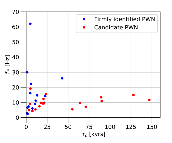
Figure 1: Spin frequency $f_{\ast}$ versus characteristic age $\tau_{c}$ of pulsars associated with TeV-bright PWNe in the TeV2 catalog [65, 66, 67, 68]. The blue dots represent pulsars associated with firmly identified (i.e., definitely) TeV-bright PWNe. The red dots show the pulsars associated with HESS candidate PWNe.

The search over 20–200 Hz is divided into 2-Hz-wide sub-bands. This ensures that loud non-Gaussian noise artifacts (e.g., lines) are confined to one sub-band and do not affect the whole analysis. Additionally, we overlap the frequency sub-bands by 0.02 Hz to ensure that there is always a sub-band that fully contains a signal, even if the source is rapidly spinning down. The 0.02 Hz overlap is sufficient to cover the maximum plausible amount of spin wandering during a typical observation of $T_{\rm obs}\lesssim 234$ days.

II.3 Coherence time

The coherence time $T_{\rm{coh}}$ sets the frequency resolution of the search. It is chosen such that a wandering signal frequency remains in one frequency bin during a single coherent step. Here, we rely on the estimated, age-based spin-down rate ($\dot{f}_{0}$) to choose an optimal $T_{\rm{coh}}$ for the search. It is estimated using [80, 53, 81]

$$-\frac{f_{0}}{(n_{\mathrm{min}}-1)\tau_{\mathrm{age}}}\leq\dot{f_{0}}\leq-\frac{f_{0}}{(n_{\mathrm{max}}-1)\tau_{\mathrm{age}}},$$ (1)

where $f_{0}$ represents the signal frequency, $\tau_{\mathrm{age}}$ is the age of the source (here assumed to be the characteristic age $\tau_{c}$), and $n_{\rm{min}}$ and $n_{\mathrm{max}}$ represent the minimum and maximum value of the braking index $n=f_{0}\ddot{f_{0}}/\dot{f_{0}}^{2}$, respectively. With $\dot{f}_{0}$ estimated according to Eq. 1, we set $T_{\rm{coh}}\leq({2|\dot{f_{0}}|})^{-1/2}$ [80, 52, 82]. A full derivation of this expression is available in Appendix A.

Multiple groups have attempted to estimate the age of HESS J1427-608. Assuming that the TeV source is an evolved PWN, Devin et al. [28] estimate a characteristic age between 4.9 and 13.6 kyr. Fujinaga et al. used the correlation between the ratio of $\gamma$-ray to x-ray flux ($F_{\gamma}/F_{X}$) and $\tau_{c}$ to obtain $\tau_{c}\sim 6.4~{}$kyr [83]. However, as reported in Ref. [84], the fit that relates $F_{\gamma}/F_{X}$ to $\tau_{c}$ has an uncertainty factor of $\sim$2.6, which increases the bounds on the estimated age to $2.5<\tau_{c}<16.5$ kyr. Additionally, the measured power-law relation between the distance-independent TeV surface brightness and spin-down power yields an age estimate of $1<\tau_{c}<20$ kyr [54]. These estimates indicate a relatively young source. Here, we use the age estimate from x-ray observations (i.e. $2.5<\tau_{c}<16.5$ kyr) as the evolution of x-ray emission is strongly correlated with the evolution of the magnetic field, which in turn depends on the morphological evolution of PWN. In contrast, the TeV $\gamma$-ray emission is from the long-lived electrons which trace the time-integrated evolution of the nebula [84].

Now we determine the range of minimum and maximum spin-down rate ($\dot{f_{0}}$) expected for a target with $f_{0}\in[20,200]$ Hz and $\tau_{c}\in[2.5,16.5]$ kyr. As the braking index is unknown for this source, we calculate $T_{\rm{coh}}$ for $n\in[2,5,7]$ to cover the extreme plausible values, based on the current observations [85, 86]. The choice of $n=2$ encompasses the broadest range of $\dot{f_{0}}$ values, while the $n=5$ and $n=7$ cases cover astrophysical scenarios where the phase evolution is purely due to GW emission and r-mode oscillations, respectively. Assuming that the frequency evolution caused by timing noise is much smaller than the secular spin-down rate of the pulsar (see Sec. V B of Ref. [82]), we use Eq. (1) to estimate the range of possible $\dot{f}_{0}$ and thus $T_{\rm{coh}}$. A list of possible values is presented in Table 1. We can cover all of the aforementioned scenarios with $T_{\rm{coh}}=4$ h. However, this $T_{\rm{coh}}$ is not optimal as a large number of data segments, $N_{T}\gtrsim 1404$, must be incoherently combined, thus degrading the sensitivity of the search which scales $\propto N_{\rm{T}}^{-1/4}$ [87]. To circumvent this issue, we choose an intermediate $T_{\rm{coh}}=7.5$ h, which corresponds to $\dot{f_{0}}\in[-6.85\times 10^{-10},6.85\times 10^{-10}]$ Hz/s. This choice of $T_{\rm{coh}}$ allows us to cover the full frequency and age ranges, if the GW emission is due to mass ($n=5$) and current ($n=7$) quadrupoles, and cover most of the interesting parameter space for $n=2$ (i.e., the entire frequency range for $9.5\leq\tau_{c}\leq 16.5$ kyr and part of the spectrum for $\tau_{c}\leq 9.5$ kyr). Signals with $\dot{f_{0}}$ outside the covered range can also be partially tracked by the HMM, although with lower sensitivity.

Table 1: Estimated $\dot{f_{0}}$ and $T_{\rm{coh}}$ in [20,200] Hz band.

$n$	$\tau_{c}$	$|\dot{f_{0}}|\$(Hz s${}^{-1})$	$T_{\rm{coh}}$ (h)
2	2.5	[2.54$\times 10^{-10}$, 2.54$\times 10^{-9}$]	[3.90, 12.33]
2	16.5	[3.84$\times 10^{-11}$, 3.84$\times 10^{-10}$]	[10.02, 32.68]
5	2.5	[6.34$\times 10^{-11}$, 6.34$\times 10^{-10}$]	[7.80, 24.66]
5	16.5	[9.61$\times 10^{-12}$, 9.61$\times 10^{-11}$]	[20.04, 63.36]
7	2.5	[4.23$\times 10^{-11}$, 4.23$\times 10^{-10}$]	[9.55, 30.21]
7	16.5	[6.41$\times 10^{-12}$, 6.41$\times 10^{-11}$]	[24.54, 77.60]

III Search procedure

The search presented here is carried out in two steps. First, the $\mathcal{F}$ statistic implementation in LALSuite [88] is used to coherently combine detector data and compute a log-likelihood score for each 7.5 h time block. Second, HMM tracking is used to find the optimal frequency path through the data over the total observing run. To be precise, the optimal path is recovered using the Viterbi algorithm, a dynamic programming implementation of a HMM. This is similar to the approach used in Refs. [50, 41, 80, 81]. The signal model is briefly reviewed in Sec. III.1, while the $\mathcal{F}$ statistic and HMM are outlined in Secs. III.2 and III.3, respectively. The procedure used for setting an appropriate threshold is described in Sec. III.4. Finally, the details of interferometric data used here are outlined in Sec. III.5.

III.1 Signal model

We use the signal model described in Ref. [49]. What follows is a summary of the most salient details. We model the wave strain from a neutron star as

$$h(t)=\mathcal{A}^{\mu}h_{\mu}(t),$$ (2)

where $\mathcal{A}_{\mu}$, which depends on characteristic strain amplitude ($h_{0}$), source orientation ($\iota$), initial phase ($\phi_{0}$), and wave polarisation ($\times$ or +), represent the amplitudes associated with four linearly independent components [49]

$$h_{1}(t) =a(t)\cos\Phi(t),$$ (3)

$$h_{2}(t) =b(t)\cos\Phi(t),$$ (4)

$$h_{3}(t) =a(t)\sin\Phi(t),$$ (5)

$$\quad h_{4}(t) =b(t)\sin\Phi(t).$$ (6)

Here, $a(t)$ and $b(t)$ are the antenna-pattern functions as defined by Eqs. (12) and (13) of Ref. [49] and $\Phi(t)$ is the phase of the CW signal of form

$$\Phi(t)=2\pi f_{0}[t+\Phi_{m}(t;\alpha,\delta)]+\Phi_{s}(t;f_{0}^{(k)},\alpha,\delta).$$ (7)

The $\Phi_{m}$ term in the above expression represents the time shift introduced by the diurnal and annual motion of the detector relative to the solar system barycenter, while the $\Phi_{s}$ is the phase shift that results from intrinsic evolution of the source in its rest frame through its frequency derivatives ($f_{0}^{(k)}=d^{(k)}f_{0}/dt^{(k)}$ with $k\geq 1$).

The intrinsic frequency evolution of a CW signal has two components: a secular term, which can be easily modeled by specifying the frequency derivatives $f_{0}^{(k)}$, estimated using the procedure outlined in Sec. II.3, and a stochastic term, which is often difficult to measure and computationally infeasible to track in a coherent search. To circumvent this issue, we use the HMM outlined in Sec. III.3 to track the stochastic evolution of the signal phase and the Viterbi algorithm to efficiently backtrack and find the optimal pathway in frequency.

III.2 $\mathcal{F}$ statistic

As in Ref. [50], we use the $\mathcal{F}$ statistic to estimate the likelihood of a CW signal being present in the detector data. The time-dependent output of a single detector is assumed to take the form [49]

$$x(t) =h(t)+n(t),$$ (8)

where $n(t)$ represents stationary, additive noise and $h(t)$ is the wave strain defined in Eq. (2). We start by defining a normalised log-likelihood of the form [49]

$$\ln\Lambda\equiv(x|h)-\frac{1}{2}(h|h),$$ (9)

where the inner product $(\cdot|\cdot)$ is a sum over single-detector inner products and is given by

$$(x|y) =\sum_{X=1}^{N_{\rm{Det}}}(x^{X}|y^{X})$$ (10)

$$\approx{\sum_{X=1}^{N_{\rm{Det}}}\frac{2}{S_{h}^{X}(f)}\int_{0}^{T_{\rm{obs}}}dt\ x^{X}(t)y^{X}(t)}.$$ (11)

Here, $N_{\rm{Det}}$ is the number of detectors and $S_{h}^{X}(f)$ represents the one-sided power spectral density (PSD) of detector $X$ at frequency $f$ [89]. We maximise $\ln\Lambda$ with respect to the four amplitude parameters $\mathcal{A_{\mu}}$ to find the optimal set of signal parameters. These parameters, known as the maximum likelihood (ML) estimators, are then used to define the $\mathcal{F}$ statistic,

$$\mathcal{F} \equiv\ln{\Lambda}_{\mathrm{ML}}$$ (12)

$$=D^{-1}[B(x|h_{1})^{2}+A(x|h_{2})^{2}-2C(x|h_{1})(x|h_{2})$$

$$\quad+B(x|h_{3})^{2}+A(x|h_{4})^{2}-2C(x|h_{3})(x|h_{4})]$$ (13)

with $A=(a|a)$, $B=(b|b)$, $C=(a|b)$, and $D=AB-C^{2}$. A full derivation can be found in Sec IIIA of Ref. [49]. In the case of white Gaussian noise with no signal, the probability density function (PDF) of the $\mathcal{F}$ statistic takes the form of a central $\chi^{2}$ distribution with 4 degrees of freedom, $p(2\mathcal{F})=\chi^{2}(2\mathcal{F};4,0)$. When a signal is present, the PDF has a non-central $\chi^{2}$ distribution with 4 degrees of freedom, $p(2\mathcal{F})=\chi^{2}(2\mathcal{F};4,\rho_{0}^{2})$, where the non-centrality parameter is given by

$${\rho_{0}}^{2}=\frac{K{h_{0}}^{2}T_{\rm{coh}}}{S_{h}(f_{0})}.$$ (14)

Here, $S_{h}(f)$ is computed as a harmonic sum over the detector-specific $S_{h}^{X}(f)$, while the constant $K$ depends on the sky location and orientation of the source [49].

III.3 HMM

In this search, we model the stochastic wandering of a CW signal frequency as a Markov chain, whereby the unobservable, hidden state variable $q(t)$ transitions between a set of discrete states $\{q_{0},q_{1},...,q_{N_{Q}}\}$ at discrete times $\{t_{0},t_{1},...,t_{N_{T}}\}$. Meanwhile, the observable state variable $o(t)$ takes values from the set {$o_{1},...,o_{N_{O}}$}. As the Markov chain is memoryless, the state of the system at time $t_{n+1}$ depends only on the state at a previous time step $t_{n}$, and the transition probability matrix is given by

$$A_{q_{j}q_{i}}=\mathrm{Pr}[q(t_{n+1})=q_{j}|q(t_{n})=q_{i}].$$ (15)

The observable state $o_{j}$ is related to the hidden state $q_{i}$ via the emission probability matrix of form

$$L_{o_{j}q_{i}}=\mathrm{Pr}[o(t_{n})=o_{j}|q(t_{n})=q_{i}].$$ (16)

Finally, the model is completed by specifying the probability of the system occupying each hidden state initially, given by the prior vector of form

$$\Pi_{q_{i}}=\mathrm{Pr}[q(t_{0})=q_{i}].$$ (17)

We then find the most probable sequence of hidden states $Q^{*}$ given observable state sequence $O$ by finding $Q$ that maximizes [50]

$$\mathrm{Pr}(Q|O) \propto L_{o(t_{N_{T}})q(t_{N_{T}})}A_{q(t_{N_{T}})q(t_{N_{T}-1})}...$$

$$\quad\times L_{o(t_{1})_{q}(t_{1})}A_{q(t_{1})}\Pi_{q}(t_{0}).$$ (18)

The Viterbi algorithm, as described in Ref. [90] and applied to CW searches in Refs. [50, 41, 81, 15], provides a recursive and computationally efficient method for computing $Q^{*}$ from Eqs. (15)–(18). For computational convenience and numerical stability, we evaluate $\mathcal{L}=\log\mathrm{Pr}(Q|O)$, whereby the products in Eq. (18) become a sum of log-likelihoods.

Here, the CW signal frequency $f_{0}(t)$ is the hidden state variable, which moves by at most one bin up or down during a timescale $T_{\rm{coh}}$. This is identical to the approach used in Refs. [50, 41, 15] and represented by the following transition matrix:

$$A_{q_{i-1}q_{i}}=A_{q_{i}q_{i}}=A_{q_{i+1}q_{i}}=\frac{1}{3},$$ (19)

with all other $A_{q_{j}q_{i}}$ entries being zero. This choice of matrix is appropriate because timing noise is especially pronounced in young pulsars with $\tau_{c}\lesssim 10$ kyr [48, 39]. The observable is the $\mathcal{F}$ statistic with an emission probability given by [50, 80]

$$L_{o_{j}q_{i}}\propto\exp{[\mathcal{F}(f_{0})]},$$ (20)

where $\mathcal{F}(f_{0})$ is computed for each segment of length $T_{\rm{coh}}$ at a frequency resolution of $\Delta f_{\rm{coh}}=1/(2T_{\rm{coh}})$. The method for setting $T_{\rm{coh}}$ is discussed in Sec. II.3. We choose a uniform prior $\Pi_{q_{i}}=N_{Q}^{-1}$ for this study, as the frequency of the signal at $t_{0}$ is unknown.

III.4 Threshold

We aim to find a threshold log-likelihood ($\mathcal{L}_{\rm{th}}$) that corresponds to a desired false alarm probability $\alpha_{f}=1\%$ in each sub-band. The detector ASD $\left[{S_{h}(f)}^{1/2}\right]$ changes by 3 orders of magnitude over the 20–200 Hz band [73]. To understand how this may affect the threshold for the search, we generate 500 Gaussian noise realizations in eight, 2-Hz-wide sub-bands, namely, those starting at 20, 45, 61, 80, 110, 145, 175, and 200 Hz. We set ${S_{h}(f)}^{1/2}$ of each sub-band to match the band-averaged one-sided noise ASD of the O2 data [73]. The search parameters are outlined in Table 2. Figure 2 shows the distributions of maximum log-likelihoods obtained using 500 realizations in each sub-band, all of which are consistent with a Gumbel distribution [91]. We list the 99th percentile $\mathcal{L}_{\rm{th}}$ corresponding to $\alpha_{f}=1\%$ for each sub-band in Table 3. The results show relatively small variation ($\sim 0.2\%$) over the 20–200 Hz frequency range. This is consistent with the results presented in Ref. [92], where a similar trend is observed despite using a slightly different detection statistic. These results also show negligible variation in the predicted $\mathcal{L}_{\rm{th}}$ with the detector noise PSD. This is expected as the inner product defined in Eq. (11) includes a noise weighting $\propto S_{h}(f)^{-1}$ that removes the dependence on $S_{h}(f)$. We therefore combine all 4000 noise realisations into a single dataset and use it to compute the 99th percentile $\mathcal{L_{\rm{th}}}$ = 5396, corresponding to $\alpha_{f}=1\%$ per 2 Hz sub-band.

Table 2: Search parameters. Here, $N_{T}=T_{\rm{obs}}/T_{\rm{coh}}$ is the total number of coherent steps. RA, right ascension: DEC, declination.

Parameter	Value	Units
RA	14:27:56.7	J2000 h:min:s
DEC	–60:52:14	J2000 deg:min:s
$f_{0}$	20–200	Hz
$\Delta f_{\rm{coh}}$	$1.9\times 10^{-5}$	Hz
$T_{\rm{coh}}$	7.5	h
$T_{\rm{obs}}$	234	days
$N_{\rm{T}}$	748	…

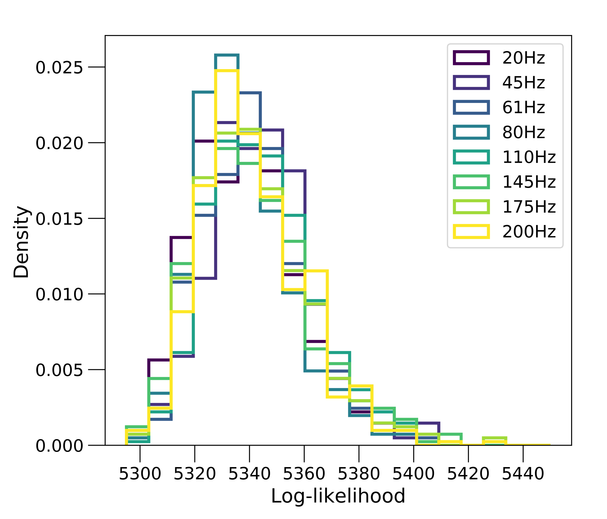
Figure 2: Distribution of maximum log-likelihood scores in Gaussian noise across eight frequency sub-bands. Each distribution is constructed using 500 realisations. The starting frequency of each 2-Hz-wide sub-band is denoted in the legend.

Table 3: The 99th percentile log-likelihood thresholds for eight sub-bands used in the threshold study.

sub-band (Hz])	$\mathcal{L}_{\rm{th}}$
20–22	5394
45–47	5402
61–63	5394
80–82	5388
110–112	5399
145–147	5399
175–177	5400
200–202	5393

III.5 LIGO data

We use the publicly available data from the O2 run of the aLIGO detectors, specifically the GWOSC-4KHz$\_$R1$\_$STRAIN channel, to search for CW signals from HESS J1427-608 [73]. The aVirgo detector was also operating for the last month of O2. However, we omit Virgo data due to the relatively short observing time and lower sensitivity [73]. We also exclude data from the first few weeks of the O2 run (November 30, 2016–January 4, 2017), where the data quality was not optimal and was followed by a brief break in the operation of both detectors. With these cuts, we choose a common period from January 4–August 25, 2017 (GPS time = 1167545066–1187762666) to perform a joint analysis of the two aLIGO detectors. This gives us a total observation period of $T_{\rm{obs}}=234$ days. Table 2 summarises the parameters of the search.

IV Results

The search returns a total of 246 candidates with $\mathcal{L}>\mathcal{L}_{\rm{th}}$ over the frequency range from 20–200 Hz. This number exceeds the single candidate expected given $\alpha_{f}=1\%$ per sub-band, most likely due to non-Gaussian features in the real aLIGO detector noise. This is especially true for sub-bands with $f_{0}<80$ Hz, which are heavily contaminated by instrumental lines and contain 94$\%$ of candidates identified here (refer to Fig. 3).

All 246 candidates are passed through a four-step veto procedure, which is adapted from previous studies [52, 92, 53] and used to eliminate candidates resulting from noise artifacts. The vetoes are as follows: (1) The known line veto rejects candidates that have a Viterbi path that intersects a known instrumental line in either the Hanford or Livingston detector. (2) The single interferometer veto eliminates candidates that return $\mathcal{L}>\mathcal{L}_{\cup}$ in only one of the interferometers, not both. Here, $\mathcal{L}_{\cup}$ denotes the log-likelihood from the dual-interferometer search. (3) The Doppler modulation (DM) veto involves turning off the DM correction, which accounts for the Doppler shift due to Earth’s motion, and recomputing the log-likelihoods. Astrophysical signals usually become undetectable without this correction [93]. Therefore, candidates with comparable $\mathcal{L}$ in both the DM-on and DM-off searches are rejected. (4) The off-target veto involves performing the search at an offset sky location. We reject candidates that return comparable $\mathcal{L}$ in both the on-target and off-target searches.

The reader is referred to Appendix B for a detailed description of all four vetoes. Table 4 summarises the outcome at each veto step, while Fig. 3 shows the location of each candidate in the log-likelihood ($\mathcal{L}$) versus frequency space. No candidates survive at the end of the veto procedure.

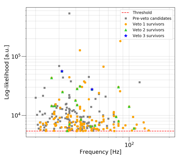
Figure 3: Log-likelihood ($\mathcal{L}$) versus frequency of candidates with $\mathcal{L}>\mathcal{L}_{\rm{th}}$. The dotted horizontal line indicates the Gaussian threshold set using the procedure outlined in Sec. III.4. The pre-veto candidates (gray squares) are shown along with the survivors after the known lines veto (orange circles), single interferometer veto (green triangles) and Doppler modulation veto (blue stars). No candidate survives the off-target veto.

Table 4: The number of candidates remaining after each post-processing step. A total of 246 candidates, with $\mathcal{L}>\mathcal{L}_{\rm{th}}$, are passed through a four-step veto procedure. None survive this procedure.

Processing step	Number of candidates
Preveto	246
Known lines veto	135
Single interferometer veto	20
Doppler modulation veto	2
Off-target veto	0

IV.1 Observational upper limits

No above-threshold candidates survive the postprocessing analysis outlined in Sec. IV. We therefore start by obtaining an estimate for the minimum detectable strain using the following analytic expression for the $95\%$ confidence sensitivity of a search [80, 94], viz.

$$h_{0}^{\rm{est}}=\Theta S_{h}(f)^{1/2}(T_{\rm{obs}}T_{\rm{coh}})^{-1/4},$$ (21)

where $S_{h}(f)^{1/2}$ is the noise ASD and $\Theta$ is the statistical threshold that is directly proportional to the root-mean-square signal-to-noise ratio of the search [87]. One typically finds $30\lesssim\Theta\lesssim 40$ for this type of search [94]. Following previous searches for CW signals with a HMM [95, 80, 94], we set $\Theta$ = 35. The theoretical upper limit ($h_{0}^{\rm{est}}$) is shown by the red curve in Fig 5.

We also quantify the sensitivity of the search by estimating $h_{0}^{95\%}$, such that a circularly polarised signal with $h_{0}\geq h_{0}^{95\%}$ is detectable on 95$\%$ or more occasions. To do this, we randomly inject 100 simulated signals with a fixed $h_{0}$ into five sub-bands, namely, those starting at 86, 101, 146, 170, and 194 Hz. These sub-bands are chosen at random from a set of bands that return less than three unique paths with $\mathcal{L}>\mathcal{L_{\rm{th}}}$ in the original search. Equation (21) provides the scaling that can be used to estimate the sensitivity of all other frequency sub-bands. Additionally, the frequencies of these software injections are randomly chosen within the sub-band. As the upper limits computed here are model dependent, we set $\cos\iota=1$ for optimal orientation and randomly draw the polarisation angle from $\psi\in[0,\pi]$. For each trial, we then use a combination of the $\mathcal{F}$ statistic and Viterbi algorithm to look for the injected signal in the detector data, using the setup outlined in Table 2. The above process is repeated for ten different values of $h_{0}$ in each sub-band. Each trial acts as a Bernoulli trial with a probability of success (efficiency) $p$ given by the Wilson interval [96],

$$p\approx\frac{s+\frac{1}{2}{(1-\alpha_{f}/2)}^{2}}{N_{I}+{(1-\alpha_{f}/2)}^{2}}\pm\frac{1-\alpha_{f}/2}{N_{I}+{(1-\alpha_{f}/2)}^{2}}\\ \sqrt{\frac{s(N_{I}-s)}{N_{I}}+\frac{{(1-\alpha_{f}/2)}^{2}}{4}},$$ (22)

where $N_{I}=100$ is the number of injections and $s$ is the number of successes. For each sub-band, we use the curve fit tool in PYTHON to fit a sigmoid curve [97] to the distribution of recovery efficiency ($p$) versus strain sensitivity ($h_{0}$), with uniform priors over the sigmoid parameters. An example fit is shown in Fig. 4. The best fit parameters are then used to find $h_{0}^{95\%}$ which corresponds to $p=95\%$. The black dots in Fig. 5 show the estimated upper limits for the five sub-bands tested here.

Finally, we calculate $a=h_{0}^{95\%}/h_{0}^{\rm{est}}$ for each of the five sub-bands tested here and use the mean $a$ across these sub-bands to estimate the sensitivity across the full frequency band as $h_{0}^{95\%}=ah_{0}^{\rm{est}}$. This is shown by the blue curve in Fig. 5.

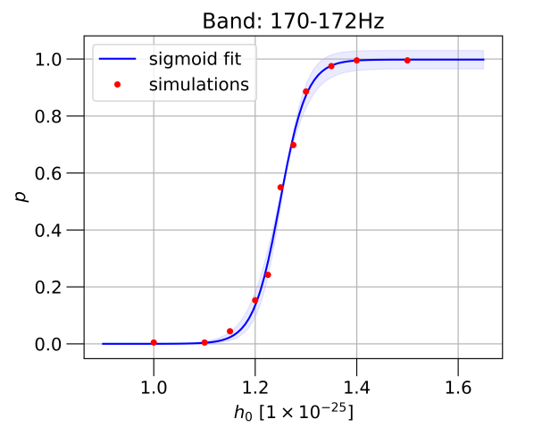
Figure 4: Detection efficiency ($p$) versus signal strain ($h_{0}$) for 170$-$172 Hz sub-band. The red dots show the results obtained with simulated signals in detector data while the solid blue curve shows the sigmoid fit along with the $2\sigma$ uncertainty interval.

The estimated search sensitivity is below the theoretical limit over the entire search band. This occurs because the search is sensitive not to $h_{0}$ but to a combination of $h_{0}$ and $\cos{\iota}$, commonly referred to as $h_{0}^{\rm{eff}}$. The scaling is given by [98]

$$\left(h_{0}^{\rm{eff}}\right)^{2}=h_{0}^{2}\frac{[(1+\cos^{2}\iota)/2]^{2}+[\cos\iota]^{2}}{2},$$ (23)

where $(h_{0}^{\rm{eff}})^{2}=h_{0}^{2}$ for circular polarisation (i.e., $\iota=0^{\circ}$ or $180^{\circ}$), $h_{0}^{2}/8$ for linear polarisation (i.e., $\iota=90^{\circ}$) and $2h_{0}^{2}/5$ for an isotropic average over the inclination angle $\iota$.

The $h_{0}^{95\%}$ limits obtained empirically in the five sample sub-bands assume $\cos{\iota}=1$ for optimal orientation (i.e., circularly polarised signals). Therefore, these limits do not need to be scaled as one has $h_{0}^{\rm{eff},95\%}=h_{0}^{95\%}$. The expression for $h_{0}^{\rm{est}}$, on the other hand, assumes marginalisation over the unknown parameters, namely $\cos{\iota}$ and $\psi$ [99, 87]. Therefore, one must scale $h_{0}^{\rm{est}}$ to obtain an effective sensitivity independent of $\cos\iota$ (i.e., $h_{0}^{\rm{eff,est}}=\sqrt{2/5}\ h_{0}^{\rm{est}}$) before comparing it to $h_{0}^{\rm{eff,95\%}}$ or $h_{0}^{\rm{95\%}}$.

The scaling ratio, which is used to compute sensitivity across the full frequency band, is thus expected to be $a=h_{0}^{\rm{eff,95\%}}/h_{0}^{\rm{eff,est}}=0.633$. Based on the simulation results, the calculated ratio (i.e., $a=0.639$) is consistent with this value within uncertainty and thus explains the observed trend.

IV.2 Theoretical upper limits

Assuming that the star loses all of its rotational kinetic energy as GWs, we can also derive an age-based indirect strain limit ($h_{0}^{\rm{age}}$) for the source, given by [95]

$$h_{0}^{\rm{age}}=2.27\times 10^{-24}\left(\frac{\rm{1~{}kpc}}{D}\right)\left(\frac{\rm{1~{}kyr}}{\tau_{c}}\right)^{\frac{1}{2}}\left(\frac{I_{zz}}{\rm{10^{38}~{}kg~{}m^{2}}}\right).$$ (24)

Here, $D$ is the distance to the source, $\tau_{c}$ is the characteristic age, and $I_{zz}$ is the principle moment of inertia. Although the exact distance to HESS J1427-608 is unknown, studies suggest a value between 6 and 11 kpc [83, 100, 28]. Assuming $I_{zz}=10^{38}$ kg m² and $\tau_{c}~{}\in~{}[2.5,16.5]$ kyr, the age-based indirect strain sensitivity is $0.51\leq h_{0}^{\rm{age}}/(10^{-25})\leq 2.39$. This is shown by the horizontal orange band in Fig. 5. Note that the 95$\%$ confidence upper limit surpasses the indirect age-based limit for $f_{0}>50$ Hz and specific source scenarios (i.e., $2.5<\tau_{c}<4$ kyr and $6<D<7.5$ kpc), reaching a minimum of $1.3\times 10^{-25}$ around 185 Hz. Data from O3 and future observing runs are needed to explore the remaining parameter space and exclude other source scenarios.

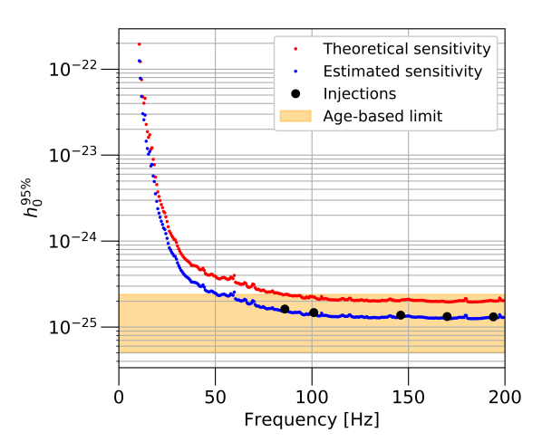
Figure 5: The sensitivity estimate $h_{0}^{95\%}$ obtained for HESS J1427-608 assuming a circularly-polarised signal. The red curve represents the minimum detectable strain derived using the analytic expression in Eq. (21). The black dots represent the $h_{0}^{95\%}$ limit obtained empirically in the sample sub-bands. The blue curve represents the estimated $h_{0}^{95\%}$ across the full 20–200 Hz band. The orange band indicates the age-based indirect limit ($h_{0}^{\rm{age}}$).

V Astrophysical implications

The GW strain upper limit can be converted into a constraint on the ellipticity of the neutron star $\epsilon$ [49] and the r-mode amplitude parameter $\alpha$ [71]. For ellipticity calculations, we assume that the CW signal frequency ($f_{0}$) is twice the rotational frequency ($2f_{\ast}$). Given the estimated $h_{0}^{95\%}$ and assuming a canonical moment of inertia ($I_{zz}=10^{38}$ kg m²), we constrain the fiducial ellipticity of the neutron star in terms of the GW frequency via [49, 94]

$$\epsilon=9.46\times 10^{-5}\left(\frac{h_{0}^{95\%}}{10^{-24}}\right)\left(\frac{D}{\rm{1~{}kpc}}\right)\left(\frac{\rm{100~{}Hz}}{f_{0}}\right)^{2}.$$ (25)

We also convert $h_{0}^{95\%}$ to a limit on the amplitude of r-mode oscillations via [101, 102]

$$\alpha\simeq 0.028\left(\frac{h_{0}^{95\%}}{10^{-24}}\right)\left(\frac{D}{\rm{1~{}kpc}}\right)\left(\frac{\rm{100~{}Hz}}{f_{0}}\right)^{3}.$$ (26)

These limits are shown in Fig. 6. The best constraints on the star’s ellipticity ($\epsilon\leq 2\times 10^{-5}$) and r-mode amplitude ($\alpha\leq 3\times 10^{-3}$) are obtained at 200 Hz. The ellipticity constraint is above the rough theoretical maximum ($\epsilon\sim 10^{-6}$) predicted for a neutron star [103, 104, 105]. The constraint on the r-mode amplitude, however, does reach the $\alpha\sim 10^{-3}$ level expected for the most detailed exploration of the nonlinear saturation mechanism [106, 107]. Data from future observing runs should provide stricter, more meaningful constraints. Note that the results presented here refer to a specific scenario with source properties $\psi\in[0,\pi]$ and $\cos\iota=1$.

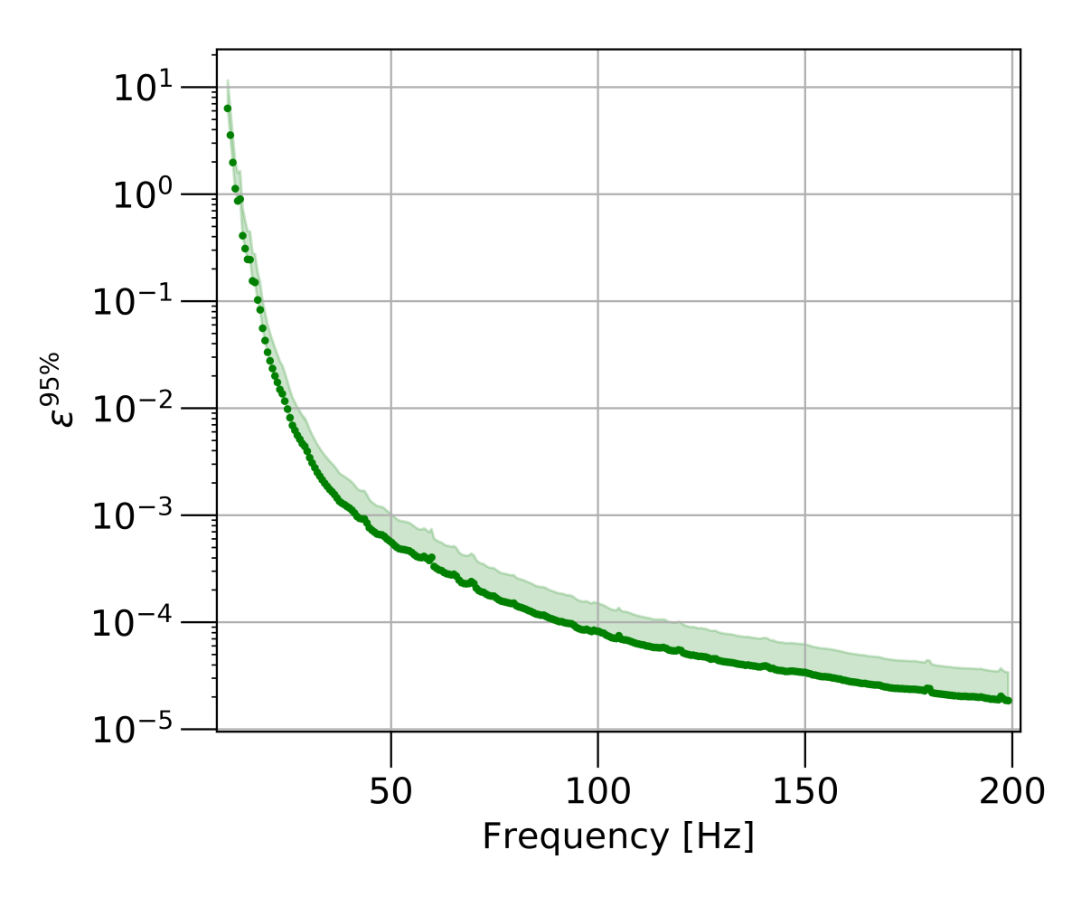
(a) Ellipticity upper limit

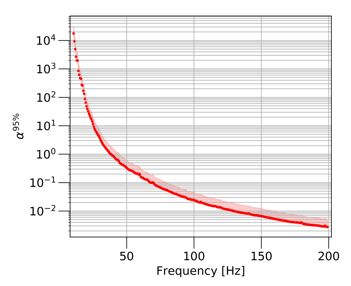
(b) R-mode amplitude upper limit

Figure 6: Constraints on the (a) neutron star ellipticity and (b) r-mode amplitude, plotted as a function of CW signal frequency ($f_{\ast}$). The red and green dotted lines correspond to the closest distance estimate (i.e., $D=6$ kpc), while the shaded regions indicate the results across the full distance range.

VI Conclusion

In this paper, we present a search for CW signals from HESS J1427-608, an unidentified and spatially unresolved TeV point source potentially harboring a young pulsar, using aLIGO’s publicly available O2 data. The search uses a method that combines the maximum likelihood $\mathcal{F}$ statistic with a HMM to efficiently track the secular spin-down and stochastic spin wandering. No evidence of a CW signal is found. We set the first upper limits on the GW signal amplitude, mass ellipticity ($\epsilon$), and r-mode amplitude ($\alpha$) for this target in a directed search. The best (lowest) constraint on the CW signal amplitude (for circularly polarized signals) is $h_{0}^{95\%}\approx 1.3\times 10^{-25}$ near 185 Hz, while $\epsilon$ and $\alpha$ are constrained to $<2\times 10^{-5}$ and $<3\times 10^{-3}$ around 200 Hz, respectively.

HESS J1427-608 has not been targeted by previous CW searches. Therefore, we cannot make a direct comparison between the results presented here and previous studies. We can, however, qualitatively compare these results with searches that target young SNRs with a compact central object ($\tau_{c}\in[2.5,16.5]$ kyr) and use O2 data. Lindblom and Owen [108] used O2 data to search for signals from 12 supernova remnants, nine of which have $\tau_{c}\in[2.5,16.5]$ kyr. No evidence of a CW signal was found. The reported strain limits are slightly above $1\times 10^{-25}$ at a 90$\%$ confidence interval level and comparable to the limit obtained here. Papa et al. [109] used O1 and O2 data to search for CW signals from the central, compact objects associated with three young supernova remnants; Cassiopeia A (Cas A), Vela Junior (Jr.) and G347.3–0.5. The authors set 90$\%$ confidence limits of $h_{0}^{90\%}=1.2\times 10^{-25},\ 9.3\times 10^{-26}\$ and $\ 9.0\times 10^{-26}$ for Cas A, Vela Junior (Jr.), and G347.3-0.5 near 185 Hz, respectively. The limits for Vela Jr. and G347.3-0.5 are $\sim 1.3$ times better than the constraint obtained here, while the Cas A limit is comparable. Following this study, Ming et al. [110] improved the constraints on the 90$\%$ upper limit for G347.3-0.5 ($\tau_{c}=1.6$ kyr) to $h_{0}^{90\%}\sim 7.5\times 10^{-26}$, which is 1.7 times better than this search, albeit for a different target [110]. However, none of the above analyses track stochastic spin wandering, unlike the HMM approach in this paper. Studies with data from future observation runs and better analysis methods will further extend the sensitivity of CW searches and increase the chances of detection.

Appendix A EXPRESSION FOR $T_{\mathrm{coh}}$

In this search, we require the change in CW signal frequency due to the secular spin-down of the pulsar over [$t,t+T_{\rm{coh}}$] to satisfy

$$\left|\int_{t}^{t+T_{\rm{coh}}}dt^{\prime}\dot{f_{0}}(t^{\prime})\right|<\Delta f_{\rm{coh}}$$ (27)

for $0<t<T_{\rm{obs}}$ [80]. Here, $T_{\rm{coh}}$ denotes the coherence timescale, $T_{\rm{obs}}$ denotes the total observation period and $\Delta{f_{\rm{coh}}}$ is the frequency resolution of the search, related to $T_{\rm{coh}}$ via

$$\Delta f_{\rm{coh}}=\frac{1}{2T_{\rm{coh}}}.$$ (28)

Even though the signal frequency $f_{0}$ may not be locked to the star’s spin frequency $f_{\ast}$ [111, 112], we can assume $\dot{f}_{0}\approx\dot{f}_{\ast}$ to a good approximation. Combining relation (27) with (28), we arrive at the following equality:

$$|\dot{f}_{*}|T_{\rm{coh}}\approx\Delta f_{\rm{coh}}=\frac{1}{2T_{\rm{coh}}}.$$ (29)

By solving for $T_{\rm{coh}}$, one obtains $T_{\rm{coh}}\leq(2|\dot{f}_{*}|)^{-1/2}$.

Appendix B VETOES

The non-Gaussian nature of interferometer noise can cause outliers with detection statistic above the threshold. To remove such artifacts, all candidates with $\mathcal{L}>\mathcal{L}_{\rm{th}}$ are passed through a four-step veto procedure. Below, we briefly describe these vetoes and their rejection criteria.

1. Instrumental noise lines. A vast majority of the terrestrial candidates are identified and rejected using the list of persistent instrumental lines [113]. These lines are identified during the detector characterization process and originate as resonant modes of the suspension system, external environmental causes and interference from the equipment around the detector. We veto all candidates for which [$f_{0}-\delta f_{0},f_{0}+\delta f_{0}$] intersects with a known instrumental line. Here, $f_{0}$ is the frequency of the path at $t=0$ and $\delta f_{0}$ is the frequency spread due to the Doppler shift correction applied by the $\mathcal{F}$ statistic, i.e., $\pm\delta f_{0}\approx 10^{-4}f_{0}$ [93].

2. Single interferometer veto. An astrophysical signal should be present in data from all detectors and have a better signal-to-noise ratio in the detector with higher sensitivity. Strong noise artifacts that are only present in one detector can also produce candidates with $\mathcal{L}>\mathcal{L}_{\rm{th}}$ in the dual-interferometer search. To separate local noise from astrophysical signals, we repeat the analysis in the Hanford and Livingston detectors individually. A candidate is vetoed if it satisfies two criteria: (1) One of the single interferometer searches yields $\mathcal{L}\geq\mathcal{L}_{\cup}$, where $\mathcal{L}_{\cup}$ denotes the log-likelihood from the dual-interferometer search, while the other interferometer yields $\mathcal{L}<\mathcal{L}_{\cup}$, and (2) the Viterbi path from the interferometer with $\mathcal{L}\geq\mathcal{L}_{\cup}$ intersects the original path.

3. Doppler modulation (DM) veto. This veto was first introduced in Ref. [114] and further studied in Refs. [53, 95, 93]. It involves turning off the DM correction, which accounts for the Doppler shift due to Earth’s motion around the Sun, and recomputing the log-likelihood [80, 53]. By default, the $\mathcal{F}$ statistic applies this correction to the data depending on the source’s sky location. It boosts the significance of a true astrophysical signal while spreading a terrestrial signal over several bins, thus reducing its significance. Therefore, we veto a candidate if the DM-off analysis yields $\mathcal{L}_{\rm{DM-off}}\geq\mathcal{L}_{\cup}$ and a new Viterbi path which intersects the band [$f_{0}-\delta f_{0},f_{0}+\delta f_{0}$], where $f_{0}$ denotes the frequency of the candidate at $t=0$. An injection study is used to test the validity of the DM veto in the search configuration presented in this paper. The results are summarized in Appendix C.

4. Off-target veto.  First introduced in Ref. [81] and further studied in Refs. [53, 95, 93], this veto involves shifting the sky position away from the true source’s location. The sky offset is related to the length of $T_{\rm{coh}}$ such that as $T_{\rm{coh}}$ increases, the offset decreases. An astrophysical candidate should yield the highest detection statistic at the source’s sky position [115]. On the contrary, a noise artifact will remain consistently above $\mathcal{L}_{\rm{th}}$ regardless of the offset. For this study, we adapt the sky offset from Ref. [82], as the coherence times are comparable. This involves shifting the right ascension by $\delta_{\rm{RA}}=3~{}\rm{h}$ and declination by $\delta_{\rm{DEC}}=10~{}\rm{min}$. We veto the candidate if the off-target search yields $\mathcal{L}_{\rm{off}}\geq\mathcal{L}_{\cup}$ and returns a new Viterbi path intersecting the band $[f_{0}-\delta f_{0},f_{0}+\delta f_{0}]$ from the dual-interferometer, DM-on search.

Appendix C DOPPLER MODULATION VETO 

We use software injections to test the effectiveness of the DM veto in separating an astrophysical signal from a terrestrial one. We start by finding a threshold log-likelihood ($\mathcal{L}_{\rm{th}}$) to give a desired false alarm probability of $\alpha_{f}=1\%$ in the 100–102 Hz sub-band. The procedure used here is identical to the one described in Sec. III.4. We generate 500 Gaussian noise-only realizations in the chosen sub-band and set the detector ASD [$S_{h}(f)^{1/2}$] to match the band-averaged one-sided noise ASD of the O2 data (see Table 5). We search the data using a combination of the $\mathcal{F}$ statistic and the Viterbi algorithm. The distribution of maximum log-likelihoods is then used to find the 99th percentile $\mathcal{L_{\rm{th}}}$ corresponding to $\alpha_{f}=1\%$.

Here, we test the validity of the DM veto using injections into Gaussian noise in two regimes: the strong signal regime, where the injected signals are easily detectable (i.e., $\mathcal{L}>>\mathcal{L}_{\rm{th}}$), and the weak signal regime, where the signals are marginally above the detection threshold (i.e., $\mathcal{L}>\mathcal{L}_{\rm{th}}$). The Gaussian thresholds for the two cases are stated in Table 6.

Once the thresholds have been established, we inject synthetic signals into white Gaussian noise. The injection parameters are outlined in Table 5. We generate 100 realisations for Hanford and Livingston detectors using the Makefakedata$\_$v4 tool in LALSuite [88]. The data are then searched using a combination of the $\mathcal{F}$ statistic and Viterbi algorithm. We summarise the parameters for this study in Table 6. These are identical to ones used in the original search. Each candidate with $\mathcal{L}\geq\mathcal{L}_{\rm{th}}$ is searched again with DM turned off and rejected if it satisfies the criteria outlined in Appendix B.

Table 5: Injection parameters used to create synthetic data analysed in the DM-veto study. rand($a,b$) denotes a uniformly distributed random number between $a$ and $b$.

Parameter	Value	Unit
Reference time	1167545066	…
RA	14:27:56.7	J2000 h:min:s
DEC	–60:52:14	J2000 deg:min:s
Band	99.9–102.1	Hz
$f_{0}$	rand(100,102)	Hz
$\cos{\iota}$	0	…
$h_{0}$	(1.5 and 3) $\times 10^{-25}$	…
$S_{h}(f)^{1/2}$	$5.6\times 10^{-24}$	$1/\sqrt{\rm{Hz}}$

Table 6: Search parameters used to test the validity of the DM veto.

Parameter	Value	Unit
Reference time	1167545066	…
RA	14:27:56.7	J2000 h:min:s
DEC	–60:52:14	J2000 deg:min:s
Band	100–102	Hz
$\Delta f$	$1.9\times 10^{-5}$	Hz
$T_{\rm{coh}}$	7.5	h
$T_{\rm{obs}}$	234	days
Threshold	5429 and 5397	…

The results are shown in Fig. 7. We experiment with two different values of $h_{0}$ to investigate the validity of DM veto in the strong and weak signal regime. The blue and red dots in Fig. 7 indicate the resultant log-likelihood with ($\mathcal{L}_{\cup}$) and without ($\mathcal{L}_{\rm{DM-off}}$) the DM correction, respectively. In the strong signal regime [Fig. 7(a)], all candidates in the DM-off search return Viterbi paths that intersect their DM-on counterpart in the band [$f_{0}-\delta f_{0}$, $f_{0}+\delta f_{0}$]. This is expected, as the injected signals have a sufficiently large signal-to-noise ratio to be easily separated from the background noise, even when the DM is turned off. However, all of these candidates have $\mathcal{L}_{\rm{DM-off}}\ll\mathcal{L}_{\cup}$, thus only satisfying one out of the two veto criteria. As a result, the injections pass the DM veto. Similarly, all candidates in the weak signal regime [Fig. 7(b)] return $\mathcal{L}_{\rm{DM-off}}<\mathcal{L}_{\rm{th}}<\mathcal{L}_{\cup}$ and thus pass the DM veto. This is true even if the analysis returns candidates with overlapping paths, as is the case for 3 out of 100 realisations. The lack of overlapping paths is expected, as the signals become indistinguishable from background noise at this strain sensitivity. These results suggest that we can safely apply the DM veto outlined in Appendix B to this search.

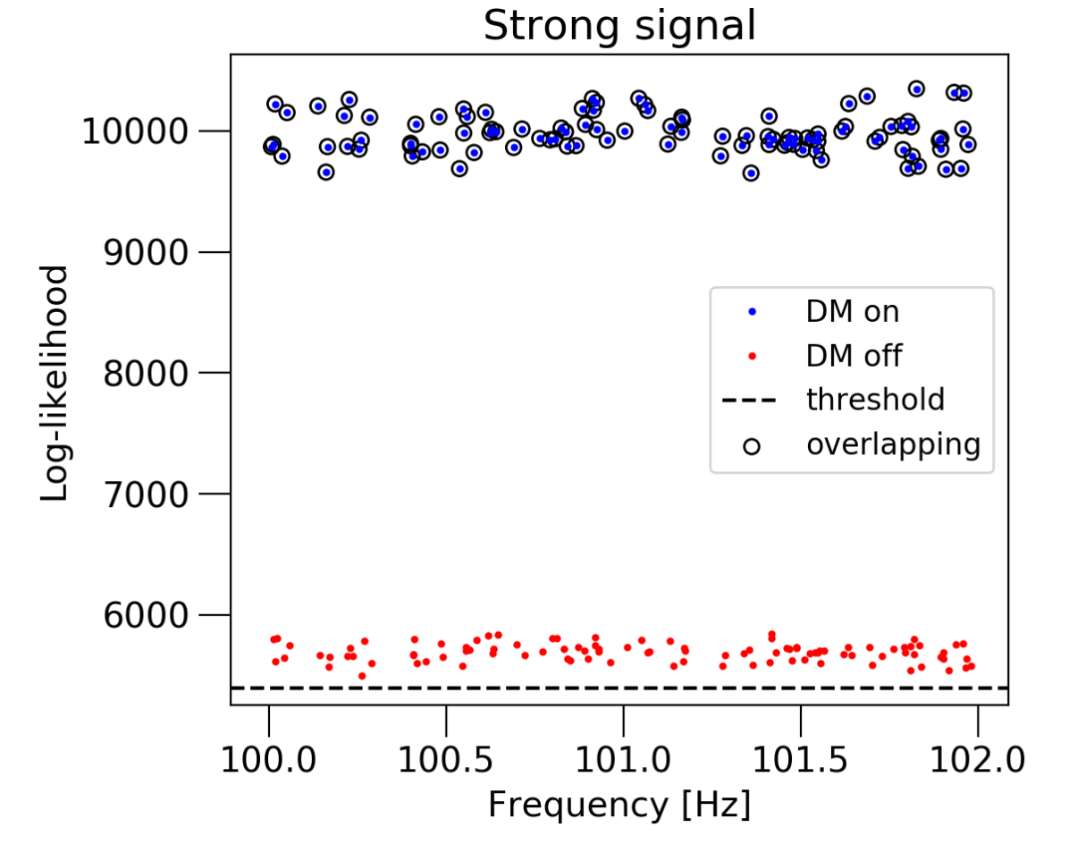
(a) Strong signal regime

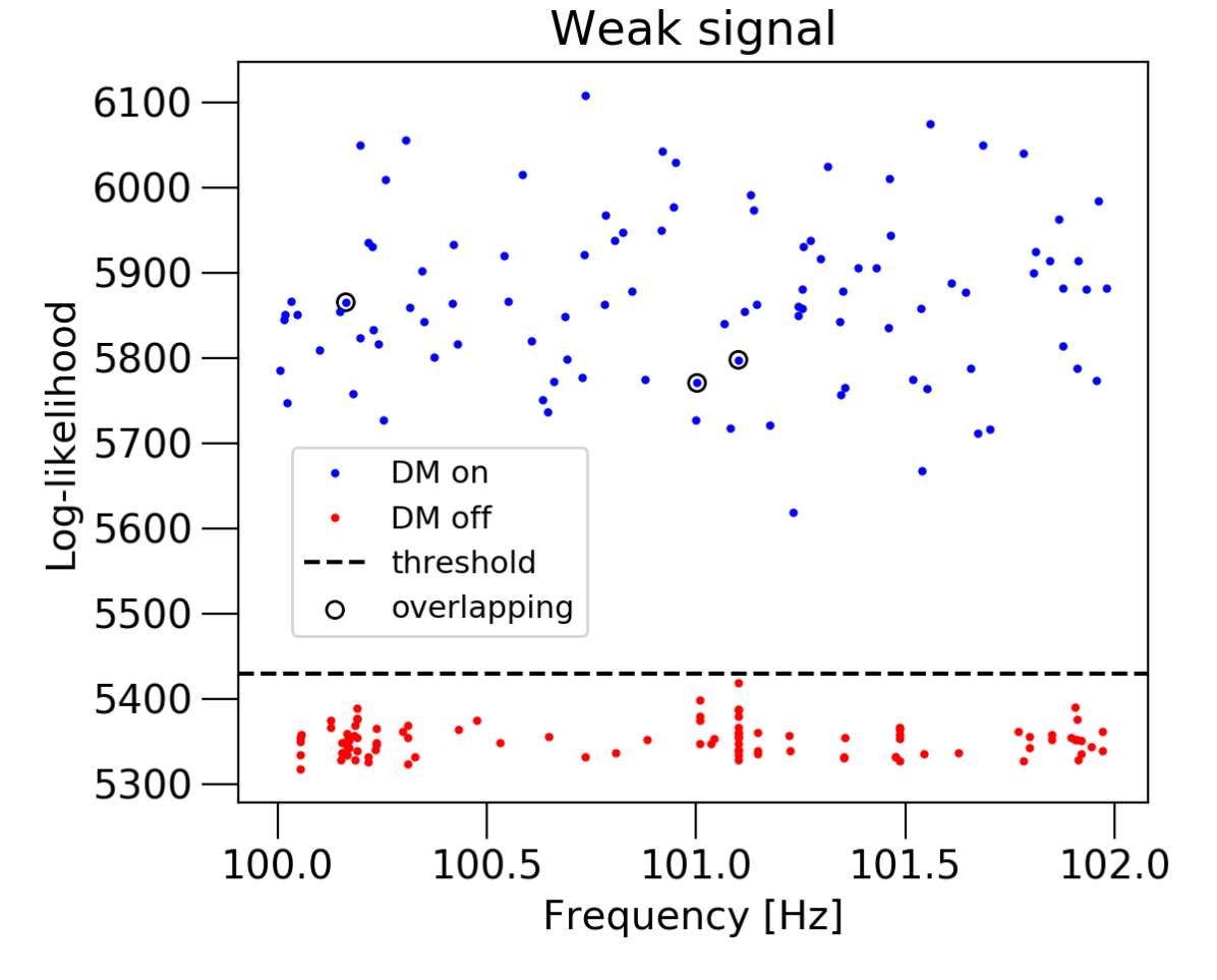
(b) Weak signal regime

Figure 7: Outcome of the Doppler modulation veto injection study, displayed as log-likelihood versus signal frequency $f_{0}$. (a) Results for the strong signal regime ($h_{0}=3\times 10^{-25}$). Blue and red dots show the results for a search with the Doppler modulation (DM) correction turned on and off, respectively. The circles indicate realisations that have overlapping paths between the two searches. (b) Weak injections ($h_{0}=1.5\times 10^{-25}$) in Gaussian noise, laid out as in (a). Note that all of the DM-off candidates are below the Gaussian threshold. Additionally, only 3/100 realisations return overlapping paths in the DM-off veto.

References

- Aasi et al. [2015] J. Aasi et al. (LIGO Scientific Collaboration), Advanced LIGO, Classical Quantum Gravity 32, 074001 (2015).
- Acernese et al. [2015] F. Acernese et al., Advanced Virgo: A second-generation interferometric gravitational wave detector, Classical Quantum Gravity 32, 024001 (2015).
- Abbott et al. [2019a] B. P. Abbott et al. (LIGO Scientific Collaboration and Virgo Collaboration), GWTC-1: A Gravitational-Wave Transient Catalog of Compact Binary Mergers Observed by LIGO and Virgo During the First and Second Observing Runs, Phys. Rev. X 9, 031040 (2019a).
- Abbott et al. [2021a] R. Abbott, T. D. Abbott, S. Abraham, F. Acernese, K. Ackley, A. Adams, C. Adams, et al. (LIGO Scientific, Virgo Collaborations), GWTC-2: Compact Binary Coalescences Observed by LIGO and Virgo During the First Half of the Third Observing Run, Phys. Rev. X 11, 021053 (2021a).
- Abbott et al. [2021b] R. Abbott et al. (LIGO Scientific, Virgo, Kagra collaborations), Observation of gravitational waves from two neutron star-black hole coalescences, Astrophys. J. Lett. 915, L5 (2021b).
- Riles [2013] K. Riles, Gravitational waves: Sources, detectors and searches, Prog. Part. Nucl. Phys. 68, 1 (2013).
- Riles [2017] K. Riles, Recent searches for continuous gravitational waves, Mod. Phys. Lett. A 32, 1730035 (2017).
- Abbott et al. [2020] R. Abbott et al. (LIGO Scientific, Virgo Collaborations), Gravitational-wave constraints on the equatorial ellipticity of millisecond pulsars, Astrophys. J. Lett. 902, L21 (2020).
- Abbott et al. [2021c] R. Abbott et al. (LIGO Scientific, Virgo, KAGRA Collaborations), Diving below the spin-down limit: Constraints on gravitational waves from the energetic young pulsar PSR J0537-6910, Astrophys. J. 913, L27 (2021c).
- Abbott et al. [2022a] R. Abbott et al. (LIGO Scientific, Virgo, KAGRA Collaborations), Searches for gravitational waves from known pulsars at two harmonics in the second and third ligo-virgo observing runs, Astrophys. J. 935, 1 (2022a).
- Abbott et al. [2022b] R. Abbott et al. (LIGO Scientific, Virgo, KAGRA Collaborations), Narrowband searches for continuous and long-duration transient gravitational waves from known pulsars in the LIGO-Virgo third observing run, Astrophys. J. 932, 133 (2022b).
- Abbott et al. [2021d] R. Abbott et al. (LIGO Scientific, Virgo, KAGRA Collaborations), Searches for continuous gravitational waves from young supernova remnants in the early third observing run of Advanced LIGO and Virgo, Astrophys. J. 921, 80 (2021d).
- Abbott et al. [2022c] R. Abbott, T. Abbott, F. Acernese, K. Ackley, C. Adams, N. Adhikari, R. Adhikari, V. Adya, C. Affeldt, D. Agarwal, et al., Search for continuous gravitational waves from 20 accreting millisecond x-ray pulsars in O3 LIGO data, Phys. Rev. D 105, 022002 (2022c).
- Abbott et al. [2022d] R. Abbott et al. (LIGO Scientific, VIRGO Collaborations), Search of the early O3 LIGO data for continuous gravitational waves from the Cassiopeia A and Vela Jr. supernova remnants, Phys. Rev. D 105, 082005 (2022d).
- Millhouse et al. [2020] M. Millhouse, L. Strang, and A. Melatos, Search for gravitational waves from 12 young supernova remnants with a hidden Markov model in Advanced LIGO’s second observing run, Phys. Rev. D 102, 083025 (2020).
- Abbott et al. [2022e] R. Abbott et al. (LIGO Scientific, Virgo and KAGRA Collaborations), Search for gravitational waves from scorpius x-1 with a hidden markov model in o3 ligo data, Phys. Rev. D 106, 062002 (2022e).
- Isi et al. [2019] M. Isi, L. Sun, R. Brito, and A. Melatos, Directed searches for gravitational waves from ultralight bosons, Phys. Rev. D 99, 084042 (2019).
- Sun et al. [2020] L. Sun, R. Brito, and M. Isi, Search for ultralight bosons in Cygnus X-1 with Advanced LIGO, Phys. Rev. D 101, 063020 (2020).
- Abbott et al. [2021e] R. Abbott et al. (LIGO Scientific, Virgo Collaborations), All-sky search in early O3 LIGO data for continuous gravitational-wave signals from unknown neutron stars in binary systems, Phys. Rev. D 103, 064017 (2021e).
- Abbott et al. [2021f] R. Abbott et al. (LIGO Scientific, Virgo, KAGRA Collaborations), All-sky search for continuous gravitational waves from isolated neutron stars in the early O3 LIGO data, Phys. Rev. D 104, 082004 (2021f).
- Abbott et al. [2019b] R. Abbott et al. (LIGO Scientific Collaboration and Virgo Collaborations), All-sky search for long-duration gravitational-wave transients in the second Advanced LIGO observing run, Phys. Rev. D 99, 104033 (2019b).
- Abbott et al. [2022f] R. Abbott et al. (The LIGO Scientific, Virgo, KAGRA Collaborations), All-sky search for gravitational wave emission from scalar boson clouds around spinning black holes in LIGO O3 data, Phys. Rev. D 105, 102001 (2022f).
- D’Antonio et al. [2018] S. D’Antonio, C. Palomba, P. Astone, S. Frasca, G. Intini, I. La Rosa, P. Leaci, S. Mastrogiovanni, A. Miller, F. Muciaccia, O. J. Piccinni, and A. Singhal, Semicoherent analysis method to search for continuous gravitational waves emitted by ultralight boson clouds around spinning black holes, Phys. Rev. D 98, 103017 (2018).
- Oliver et al. [2019] M. Oliver, D. Keitel, and A. M. Sintes, Adaptive transient hough method for long-duration gravitational wave transients, Phys. Rev. D 99, 104067 (2019).
- Dergachev and Papa [2019] V. Dergachev and M. A. Papa, Sensitivity Improvements in the Search for Periodic Gravitational Waves Using O1 LIGO Data, Phys. Rev. Lett. 123, 101101 (2019).
- Palomba et al. [2019] C. Palomba, S. D’Antonio, P. Astone, S. Frasca, G. Intini, I. La Rosa, P. Leaci, S. Mastrogiovanni, A. L. Miller, F. Muciaccia, O. J. Piccinni, L. Rei, and F. Simula, Direct Constraints on the Ultralight Boson Mass from Searches of Continuous Gravitational Waves, Phys. Rev. Lett. 123, 171101 (2019).
- Aharonian et al. [2008] F. Aharonian et al., HESS very-high-energy gamma-ray sources without identified counterparts, Astron. Astrophys. 477, 353 (2008).
- Devin et al. [2021] J. Devin, M. Renaud, M. Lemoine-Goumard, and G. Vasileiadis, Multiwavelength constraints on the unidentified Galactic TeV sources HESS J1427-608, HESS J1458-608, and new VHE -ray source candidates, Astron. Astrophys. 647, A68 (2021).
- Webb et al. [2020] N. A. Webb et al., The XMM-Newton serendipitous survey IX. The fourth XMM-Newton serendipitous source catalogue, Astron. Astrophys. 641, A136 (2020).
- Fujinaga et al. [2013] T. Fujinaga et al., An X-ray counterpart of HESS J1427-608 discovered with Suzaku, Publ. Astron. Soc. Jap. 65, 61 (2013), arXiv:1301.5274 [astro-ph.HE] .
- Abramowski et al. [2011a] A. Abramowski et al., Discovery of the source HESS J1356-645 associated with the young and energetic PSR J1357-6429, Astron. Astrophys. 533, A103 (2011a).
- Chugunov and Horowitz [2010] A. I. Chugunov and C. J. Horowitz, Breaking stress of neutron star crust, Mon. Not. R. Astron. Soc. 407, L54 (2010).
- Knispel and Allen [2008] B. Knispel and B. Allen, Blandford’s argument: The strongest continuous gravitational wave signal, Phys. Rev. D 78, 044031 (2008).
- Wette et al. [2010] K. Wette, M. Vigelius, and A. Melatos, Sinking of a magnetically confined mountain on an accreting neutron star, Mon. Not. R. Astron. Soc. 402, 1099 (2010).
- Harding and Muslimov [1998] A. K. Harding and A. G. Muslimov, Particle acceleration zones above pulsar polar caps: Electron and positron pair formation fronts, Astrophys. J. 508, 328 (1998).
- Harding and Muslimov [2002] A. K. Harding and A. Muslimov, Pulsar polar cap heating and surface thermal x-ray emission. II. Inverse Compton radiation pair fronts, Astrophys. J. 568, 862 (2002).
- Levinson et al. [2005] A. Levinson, D. Melrose, A. Judge, and Q. Luo, Large-amplitude, pair-creating oscillations in pulsar and black hole magnetospheres, Astrophys. J. 631, 456 (2005).
- Muslimov and Harding [2003] A. G. Muslimov and A. K. Harding, Extended acceleration in slot gaps and pulsar high-energy emission, Astrophys. J. 588, 430 (2003).
- Hobbs et al. [2010] G. Hobbs, A. G. Lyne, and M. Kramer, An analysis of the timing irregularities for 366 pulsars, Mon. Not. R. Astron. Soc. 402, 1027 (2010).
- Ashton et al. [2015] G. Ashton, D. I. Jones, and R. Prix, Effect of timing noise on targeted and narrow-band coherent searches for continuous gravitational waves from pulsars, Phys. Rev. D 91, 062009 (2015).
- Suvorova et al. [2017] S. Suvorova, P. Clearwater, A. Melatos, L. Sun, W. Moran, and R. J. Evans, Hidden Markov model tracking of continuous gravitational waves from a binary neutron star with wandering spin. II. Binary orbital phase tracking, Phys. Rev. D 96, 102006 (2017).
- Lyne et al. [2010] A. Lyne, G. Hobbs, M. Kramer, I. Stairs, and B. Stappers, Switched magnetospheric regulation of pulsar spin-down, Science 329, 408 (2010).
- Janssen and Stappers [2006] G. H. Janssen and B. W. Stappers, 30 Glitches in slow pulsars, Astron. Astrophys. 457, 611 (2006).
- Price et al. [2012] S. Price, B. Link, S. Shore, and D. Nice, Time-correlated structure in spin fluctuations in pulsars, Mon. Not. R. Astron. Soc. 426, 2507 (2012).
- Melatos and Link [2013] A. Melatos and B. Link, Pulsar timing noise from superfluid turbulence, Mon. Not. R. Astron. Soc. 437, 21 (2013).
- Cheng [1987] K. S. Cheng, Could glitches inducing magnetospheric fluctuations produce low-frequency pulsar timing noise?, Astrophys. J. 321, 805 (1987).
- Urama et al. [2006] J. O. Urama, B. Link, and J. M. Weisberg, A strong correlation in radio pulsars with implications for torque variations, Mon. Not. R. Astron. Soc. 370, L76 (2006).
- Arzoumanian et al. [1994] Z. Arzoumanian, D. Nice, J. Taylor, and S. Thorsett, Timing behavior of 96 radio pulsars, Astrophys. J. 422, 671 (1994).
- Jaranowski et al. [1998] P. Jaranowski, A. Krolak, and B. F. Schutz, Data analysis of gravitational-wave signals from spinning neutron stars. I. The signal and its detection, Phys. Rev. D 58, 063001 (1998).
- Suvorova et al. [2016] S. Suvorova, L. Sun, A. Melatos, W. Moran, and R. J. Evans, Hidden Markov model tracking of continuous gravitational waves from a neutron star with wandering spin, Phys. Rev. D 93, 123009 (2016).
- Quinn and Hannan [2001] B. G. Quinn and E. J. Hannan, The Estimation and Tracking of Frequency, Cambridge Series in Statistical and Probabilistic Mathematics (Cambridge University Press, Cambridge, England, 2001).
- Abbott et al. [2017] B. P. Abbott et al. (LIGO Scientific, Virgo Collaborations), Search for gravitational waves from Scorpius X-1 in the first Advanced LIGO observing run with a hidden Markov model, Phys. Rev. D 95, 122003 (2017).
- Jones and Sun [2021] D. Jones and L. Sun, Search for continuous gravitational waves from Fomalhaut b in the second Advanced LIGO observing run with a hidden Markov model, Phys. Rev. D 103, 023020 (2021).
- Abdalla et al. [2018] H. Abdalla et al. (HESS Collaboration), The population of TeV pulsar wind nebulae in the H.E.S.S. Galactic Plane Survey, Astron. Astrophys. 612, A2 (2018).
- Vigelius et al. [2007] M. Vigelius, A. Melatos, S. Chatterjee, B. M. Gaensler, and P. Ghavamian, Three-dimensional hydrodynamic simulations of asymmetric pulsar wind bow shocks, Mon. Not. R. Astron. Soc. 374, 793 (2007).
- Note [1] These refer to the soft x rays emitted from polar caps, which are heated by the bombardment of relativistic particles streaming back to the surface from the magnetosphere.
- Note [2] This refers to the emission from relativistic charged particles being accelerated in the pulsar magnetosphere.
- Becker [2009] W. Becker, X-ray emission from pulsars and neutron stars, in Neutron Stars and Pulsars, edited by W. Becker (Springer Berlin Heidelberg, Berlin, Heidelberg, 2009) pp. 91–140.
- Prinz and Becker [2015] T. Prinz and W. Becker, A search for x-ray counterparts of radio pulsars (2015), arXiv:1511.07713 .
- Marelli et al. [2015] M. Marelli, R. P. Mignani, A. De Luca, P. M. Saz Parkinson, D. Salvetti, P. R. Den Hartog, and M. T. Wolff, Radio-quiet and radio-loud pulsars: similar in Gamma-rays but different in x-rays, Astrophys. J. 802, 78 (2015).
- Gaensler and Slane [2006] B. M. Gaensler and P. O. Slane, The evolution and structure of pulsar wind nebulae, Annu. Rev. Astron. Astrophys. 44, 17 (2006).
- Hwang et al. [2004] U. Hwang et al., A million second Chandra view of Cassiopeia A, Astrophys. J. 615, L117 (2004).
- Weisskopf et al. [2000] M. C. Weisskopf et al., Discovery of spatial and spectral structure in the x-ray emission from the Crab Nebula, Astrophys. J. Lett. 536, L81 (2000).
- Santos-Lleo et al. [2009] M. Santos-Lleo, N. Schartel, H. Tananbaum, W. Tucker, and M. C. Weisskopf, The first decade of science with Chandra and XMM-Newton, Nature (London) 462, 997 (2009).
- Wakely and Horan [2014] S. Wakely and D. Horan, Tevcat 2.0, http://tevcat2.uchicago.edu (2014).
- Camilo et al. [2001] F. Camilo, J. F. Bell, et al., PSR J1016-5857: A young radio pulsar with possible supernova remnant, x-ray, and gamma-ray associations, Astrophys. J. 557, L51 (2001).
- Acero et al. [2013] F. Acero et al., Constraints on the Galactic population of TeV pulsar wind nebulae using fermi large area telescope observations, Astrophys. J. 773, 77 (2013).
- Manchester et al. [2005] R. N. Manchester, G. B. Hobbs, A. Teoh, and M. Hobbs, The Australia telescope national facility pulsar catalogue, Astrophys. J. 129, 1993 (2005).
- Ushomirsky et al. [2000] G. S. Ushomirsky, C. Cutler, and L. Bildsten, Deformations of accreting neutron star crusts and gravitational wave emission, Mon. Not. R. Astron. Soc. 319, 902 (2000).
- Melatos and Payne [2005] A. Melatos and D. J. B. Payne, Gravitational radiation from an accreting millisecond pulsar with a magnetically confined mountain, Astrophys. J. 623, 1044 (2005).
- Owen et al. [1998] B. J. Owen, L. Lindblom, C. Cutler, B. F. Schutz, A. Vecchio, and N. Andersson, Gravitational waves from hot young rapidly rotating neutron stars, Phys. Rev. D 58, 084020 (1998).
- Jones and Andersson [2001] D. I. Jones and N. Andersson, Freely precessing neutron stars: model and observations, Mon. Not. R. Astron. Soc. 324, 811 (2001).
- Abbott et al. [2021g] R. Abbott et al. (LIGO Scientific, Virgo), Open data from the first and second observing runs of Advanced LIGO and Advanced Virgo, SoftwareX 13, 100658 (2021g).
- Cahillane et al. [2017] C. Cahillane, J. Betzwieser, D. A. Brown, E. Goetz, E. D. Hall, K. Izumi, S. Kandhasamy, S. Karki, J. S. Kissel, G. Mendell, R. L. Savage, D. Tuyenbayev, A. Urban, A. Viets, M. Wade, and A. J. Weinstein, Calibration uncertainty for Advanced LIGO’s first and second observing runs, Phys. Rev. D 96, 102001 (2017).
- Abramowski et al. [2011b] A. Abramowski et al. (HESS Collaboration), Very-high-energy gamma-ray emission from the direction of the Galactic globular cluster Terzan 5, Astron. Astrophys. 531, L18 (2011b).
- Hooper and Linden [2022] D. Hooper and T. Linden, Evidence of TeV halos around millisecond pulsars, Phys. Rev. D 105, 103013 (2022).
- Lee et al. [2018] J. Lee, C. Y. Hui, J. Takata, A. K. H. Kong, P. H. T. Tam, and K. S. Cheng, X-ray census of millisecond pulsars in the Galactic field, Astrophys. J. 864, 23 (2018).
- Zhao and Heinke [2022] J. Zhao and C. O. Heinke, A census of x-ray millisecond pulsars in globular clusters, Mon. Not. R. Astron. Soc. 511, 5964 (2022).
- Caraveo [2014] P. A. Caraveo, Gamma-ray pulsar revolution, Ann. Rev. Astron. Astrophys. 52, 211 (2014).
- Sun et al. [2018] L. Sun, A. Melatos, S. Suvorova, W. Moran, and R. J. Evans, Hidden Markov model tracking of continuous gravitational waves from young supernova remnants, Phys. Rev. D 97, 043013 (2018).
- Middleton et al. [2020] H. Middleton, P. Clearwater, A. Melatos, and L. Dunn, Search for gravitational waves from five low mass x-ray binaries in the second Advanced LIGO observing run with an improved hidden Markov model, Phys. Rev. D 102, 023006 (2020).
- Beniwal et al. [2021] D. Beniwal, P. Clearwater, L. Dunn, A. Melatos, and D. Ottaway, Search for continuous gravitational waves from ten H.E.S.S. sources using a hidden Markov model, Phys. Rev. D 103, 083009 (2021).
- Fujinaga et al. [2012] T. Fujinaga, K. Mori, S. Kimura, A. Bamba, T. Dotani, M. Ozaki, H. Uchiyama, H. Matsumoto, Y. Terada, and G. PÃŒhlhofer, Suzaku observation of the VHE gamma-ray source HESS J1427-608, AIP Conf. Proc. 1427, 280 (2012).
- Mattana et al. [2009] F. Mattana, M. Falanga, D. Götz, R. Terrier, P. Esposito, A. Pellizzoni, A. De Luca, V. Marandon, A. Goldwurm, and P. Caraveo, The evolution of the - and x-ray luminosities of pulsar wind nebulae, Astrophys. J. 694, 12 (2009).
- Melatos [1997] A. Melatos, Spin-down of an oblique rotator with a current-starved outer magnetosphere, Mon. Not. R. Astron. Soc. 288, 1049 (1997).
- Archibald et al. [2016] R. F. Archibald et al., A high braking index for a pulsar, Astrophys. J. Lett. 819, L16 (2016).
- Wette [2012] K. Wette, Estimating the sensitivity of wide-parameter-space searches for gravitational-wave pulsars, Phys. Rev. D 85, 042003 (2012).
- LIGO Scientific Collaboration [2018] LIGO Scientific Collaboration, LIGO Algorithm Library - LALSuite, free software (GPL) (2018).
- Prix [2007] R. Prix, Search for continuous gravitational waves: Metric of the multidetector F-statistic, Phys. Rev. D 75, 023004 (2007).
- Viterbi [1967] A. Viterbi, Error bounds for convolutional codes and an asymptotically optimum decoding algorithm, IEEE Trans. Inf. Theory 13, 260 (1967).
- Tenorio et al. [2022] R. Tenorio, L. M. Modafferi, D. Keitel, and A. M. Sintes, Empirically estimating the distribution of the loudest candidate from a gravitational-wave search, Phys. Rev. D 105, 044029 (2022).
- Abbott et al. [2019c] B. P. Abbott et al., Search for gravitational waves from Scorpius X-1 in the second Advanced LIGO observing run with an improved hidden Markov model, Phys. Rev. D 100, 122002 (2019c).
- Jones et al. [2022] D. Jones et al., Validating continuous gravitational-wave candidates based on Doppler modulation (2022), arXiv:2203.14468 .
- Wette et al. [2008] K. Wette et al. (LIGO Scientific Collaboration), Searching for gravitational waves from Cassiopeia A with LIGO, Class. Quant. Grav. 25, 235011 (2008).
- Abbott et al. [2021h] R. Abbott et al. (LIGO Scientific, Virgo, KAGRA Collaborations), Searches for continuous gravitational waves from young supernova remnants in the early third observing run of Advanced LIGO and Virgo, Astrophys. J. 921, 80 (2021h).
- Wilson [1927] E. B. Wilson, Probable inference, the law of succession, and statistical inference, J. Am. Stat. Assoc. 22, 209 (1927).
- Banagiri et al. [2019] S. Banagiri, L. Sun, M. W. Coughlin, and A. Melatos, Search strategies for long gravitational-wave transients: Hidden Markov model tracking and seedless clustering, Phys. Rev. D 100, 024034 (2019).
- Messenger et al. [2015] C. Messenger, H. J. Bulten, S. G. Crowder, V. Dergachev, D. K. Galloway, E. Goetz, R. J. G. Jonker, P. D. Lasky, G. D. Meadors, A. Melatos, S. Premachandra, K. Riles, L. Sammut, E. H. Thrane, J. T. Whelan, and Y. Zhang, Gravitational waves from Scorpius X-1: A comparison of search methods and prospects for detection with advanced detectors, Phys. Rev. D 92, 023006 (2015).
- Wette [2009] K. W. Wette, Gravitational waves from accreting neutron stars and Cassiopeia A, Ph.D., Australian Natl. U., Canberra (2009).
- Venter et al. [2018] C. Venter, A. Harding, and I. Grenier, High-energy emission properties of pulsars, Proc. Sci. MULTIF2017, 038 (2018).
- Owen [2010] B. J. Owen, How to adapt broad-band gravitational-wave searches for -modes, Phys. Rev. D 82, 104002 (2010).
- Lindblom et al. [1998] L. Lindblom, B. J. Owen, and S. M. Morsink, Gravitational Radiation Instability in Hot Young Neutron Stars, Phys. Rev. Lett. 80, 4843 (1998).
- Johnson-McDaniel and Owen [2013] N. K. Johnson-McDaniel and B. J. Owen, Maximum elastic deformations of relativistic stars, Phys. Rev. D 88, 044004 (2013).
- Baiko and Chugunov [2018] D. A. Baiko and A. I. Chugunov, Breaking properties of neutron star crust, Mon. Not. R. Astron. Soc. 480, 5511 (2018).
- Gittins and Andersson [2021] F. Gittins and N. Andersson, Modelling neutron star mountains in relativity, Mon. Not. R. Astron. Soc. 507, 116 (2021).
- Bondarescu et al. [2009] R. Bondarescu, S. A. Teukolsky, and I. Wasserman, Spinning down newborn neutron stars: Nonlinear development of the r-mode instability, Phys. Rev. D 79, 104003 (2009).
- Haskell [2015] B. Haskell, R-modes in neutron stars: Theory and observations, Int. J. Mod. Phys. E 24, 1541007 (2015).
- Lindblom and Owen [2020] L. Lindblom and B. J. Owen, Directed searches for continuous gravitational waves from twelve supernova remnants in data from Advanced LIGO’s second observing run, Phys. Rev. D 101, 083023 (2020).
- Papa et al. [2020] M. A. Papa, J. Ming, E. V. Gotthelf, B. Allen, R. Prix, V. Dergachev, H.-B. Eggenstein, A. Singh, and S. J. Zhu, Search for continuous gravitational waves from the central compact objects in supernova remnants Cassiopeia A, Vela Jr., and G347.3-0.5, Astrophys. J. 897, 22 (2020).
- Ming et al. [2022] J. Ming, M. A. Papa, H.-B. Eggenstein, B. Machenschalk, B. Steltner, R. Prix, B. Allen, and O. Behnke, Results From an Einstein@Home search for continuous gravitational waves from G347.3 at low frequencies in LIGO O2 data, Astrophys. J. 925, 8 (2022).
- Link and Epstein [1991] B. Link and R. Epstein, Mechanics and energetics of vortex unpinning in neutron stars, Astrophys. J. 373, 592 (1991).
- Melatos [2012] A. Melatos, Fast fossil rotation of neutron star cores, Astrophys. J. 761, 32 (2012).
- Covas et al. [2018] P. B. Covas et al. (LSC Instrument Authors), Identification and mitigation of narrow spectral artifacts that degrade searches for persistent gravitational waves in the first two observing runs of Advanced LIGO, Phys. Rev. D 97, 082002 (2018).
- Zhu et al. [2017] S. J. Zhu, M. A. Papa, and S. Walsh, New veto for continuous gravitational wave searches, Phys. Rev. D 96, 124007 (2017).
- Isi et al. [2020] M. Isi, S. Mastrogiovanni, M. Pitkin, and O. J. Piccinni, Establishing the significance of continuous gravitational-wave detections from known pulsars, Phys. Rev. D 102, 123027 (2020).