The Sparse(st) Optimization Problem: Reformulations, Optimality, Stationarity, and Numerical Results

Abstract. We consider the sparse optimization problem with nonlinear constraints and an objective function, which is given by the sum of a general smooth mapping and an additional term defined by the $\ell_{0}$-quasi-norm. This term is used to obtain sparse solutions, but difficult to handle due to its nonconvexity and nonsmoothness (the sparsity-improving term is even discontinuous). The aim of this paper is to present two reformulations of this program as a smooth nonlinear program with complementarity-type constraints. We show that these programs are equivalent in terms of local and global minima and introduce a problem-tailored stationarity concept, which turns out to coincide with the standard KKT conditions of the two reformulated problems. In addition, a suitable constraint qualification as well as second-order conditions for the sparse optimization problem are investigated. These are then used to show that three Lagrange-Newton-type methods are locally fast convergent. Numerical results on different classes of test problems indicate that these methods can be used to drastically improve sparse solutions obtained by some other (globally convergent) methods for sparse optimization problems.

Keywords. Sparse optimization; global minima; local minima; strong stationarity; Lagrange-Newton method; quadratic convergence; B-subdifferential.

1 Introduction

The sparse(st) optimization problem considered in this paper is the constrained problem

$$\min_{x}f(x)+\rho\lVert x\rVert_{0}\quad\text{s.t.}\quad x\in X,$$ (SPO)

with a parameter $\rho>0$, a feasible set $X$ (usually) given by

$$X=\{x\in\mathbb{R}^{n}\mid g(x)\leq 0,\;h(x)=0\}$$

with (at least) continuous functions $f:\mathbb{R}^{n}\to\mathbb{R}$, $g:\mathbb{R}^{n}\to\mathbb{R}^{m}$, $h:\mathbb{R}^{n}\to\mathbb{R}^{p}$ and $\lVert x\rVert_{0}$ being the number of nonzero components $x_{i}$ of the vector $x$. Following standard terminology, we call $\lVert x\rVert_{0}$ the $\ell_{0}$-norm throughout this manuscript though it is not a norm. Typical applications, where sparse solutions of a given optimization problem are required, include compressed sensing for sparse representation of signals or image data, sparse portfolio selection problems, feature selection in classification learning, sparse regression or the sparse principal component analysis, see [30, Section 2] for an overview and references.

Following [22], the solution methods for problems like SPO can be divided into the following three categories: (a) convex approximations, (b) nonconvex approximations, and (c) nonconvex exact reformulations.

The most common convex approximation technique uses the $\ell_{1}$-norm instead of the $\ell_{0}$-norm in SPO. An overview on such $\ell_{1}$-surrogate models, their advantages ans solution approaches can be found in [30, Section 4.1]. Provided that $f$ and $X$ themselves are convex, the resulting optimization problem is convex (though nonsmooth) and can therefore be solved by a variety of methods for convex optimization, see [1]. This approach is very popular, for example, in solving compressed sensing problems. On the other hand, there exist prominent applications, where the $\ell_{1}$-norm provides absolutely no sparsity (like the portfolio optimization problem used in our numerical section).

This drawback leads to other sparsity improving terms that result in nonconvex approximation schemes. A natural choice is to use the $\ell_{p}$-quasi-norm for some $p\in(0,1)$, which is no longer convex, but still continuous, see [18]. Despite its nonconvexity, if there are no constraints (i.e., $X=\mathbb{R}^{n}$), the resulting problem can still be solved relatively efficiently by a proximal-type method. For additional constraints, one can apply an augmented Lagrangian-type method and use the proximal-type approach to solve the resulting (unconstrained) subproblems, see [9, 12]. In principle, these techniques can also be used for the $\ell_{0}$-norm, but the discontinuity still causes some trouble and typically leads to slowly convergent (proximal-type) gradient methods, see [12]. Another method belonging to the class of nonconvex approximations is the penalty decomposition method [24], which introduces an additional variable and solves the resulting problem by an alternating minimization technique. Also the DC-type methods (DC = difference of convex) described in [22] result in a nonconvex approximation which is shown to be exact under some additional assumptions, see also the DC-reformulation of the $\ell_{0}$-norm from [19] (this reformulation, however, is applied to cardinality-constrained problems where the $\ell_{0}$-term is not in the objective function but in the constraints, see below for a more detailed discussion).

Finally, regarding the class (c) of exact nonconvex reformulations, there are, to the best of our knowledge, still just a very few papers providing such reformulations. A natural choice is to use a mixed-integer program, cf. reformulation MIP. This is useful for finding sparse solutions of – often quadratic – problems, whose dimension is not too large, and allows, in principle, to compute a global minimum, see e.g. [2]. By modifying the objective function with a suitable regularizing term, c.f. [3], also larger problem dimensions can be handled. For nonlinear programs or large-scale problems, however, this typically leads to an intractable reformulation. One alternative approach is the complementarity-type reformulation suggested in [15], which can be shown to be completely equivalent to the original sparse optimization problem SPO. The focus of the paper [15], however, is slightly different.

More precisely, in this paper, we present two reformulations of the general sparse optimization problem SPO. These reformulations are introduced in Section 2, and partially motivated by a related approach from [5, 7] for cardinality-constrained optimization problems, cf. the corresponding discussion in Section 2. One of the two reformulations is exactly the one from [15] that we already mentioned previously. Note that the subsequent results shown for our two reformulated problems are even new for the approach from [15]. In particular, we verify in Section 3 that problem SPO and our two reformulations are equivalent in terms of both local and global minima. Section 3 introduces a problem-tailored strong stationarity concept and a corresponding constraint qualification and shows that these correspond to the standard KKT conditions and a standard constraint qualification of the two reformulated problems. We then discuss suitably adapted second-order conditions in Section 5.

Though the main goal of this paper is to lay the foundations of two exact nonconvex reformulations of the sparse optimization problem SPO, the corresponding discussion leads, in a very natural way, to Lagrange-Newton-type methods for the solution of SPO, see Section 6. Like all Newton-type methods, this is primarily a locally (fast) convergent algorithm, whereas a central difficulty for the solution of sparse optimization problems is to design suitable globally convergent methods. Nevertheless, the corresponding numerical results in Section 7 indicate that the Lagrange-Newton-type methods can be used to obtain significant improvements over solutions calculated by other (globally convergent) sparse solvers. We close with some final remarks in Section 8.

Notation: Throughout this manuscript, $e_{i}\in\mathbb{R}^{n}$ denotes the $i$-th unit vector, whereas $e:=(1,\ldots,1)^{T}\in\mathbb{R}^{n}$ is the all-one vector. Given $x\in\mathbb{R}^{n}$ and $x^{*}\in X$, we define the index sets

$$I_{0}(x):=\{i\ |\ x_{i}=0\}\quad\text{and}\quad I_{g}(x^{*}):=\{i\ |\ g_{i}(x^{*})=0\}$$

of zero components of $x$ and active inequality constraints at $x^{*}$, respectively. For an arbitrary vector $x$, we write $\text{diag}(x)$ for the corresponding diagonal matrix, whose diagonal entries are given by the elements of $x$. Given two vectors $x,y\in\mathbb{R}^{n}$, the Hadamard (elementwise) product is denoted by $x\circ y$, i.e., the elements of this vector are given by $x_{i}\cdot y_{i}$ for all $i=1,\ldots,n$.

2 Two Smooth Reformulations of SPO

In this section we derive two smooth reformulations of SPO and show that the local and global minima of these reformulated problems coincide with the local and global minima of the original sparse optimization problem SPO. One of these reformulations is already known from [15], whereas the other one is new and will be more suited for our numerical experiments later on. Note that the results stated in this manuscript for the known formulation from [15] are still new and not contained in that reference. Throughout this section, we only require $f,g,h$ to be continuous.

Let us consider the sparse optimization problem from SPO with an arbitrary set $X\subseteq\mathbb{R}^{n}$. For any $x\in\mathbb{R}^{n}$, define a corresponding binary variable $y\in\{0,1\}^{n}$ by setting $y_{i}:=0$ for $x_{i}\neq 0$ and $y_{i}:=1$ for $x_{i}=0$. Using this $y$, we can calculate the $\ell_{0}$-norm of $x$ as

$$\|x\|_{0}=\sum_{x_{i}\neq 0}1=\sum_{i=1}^{n}(1-y_{i})=n-e^{T}y.$$

Thus, we could rewrite problem SPO by the following mixed-integer problem

$$\min_{x,y}f(x)+\rho(n-e^{T}y)\quad\text{s.t.}\quad x\in X,\;x\circ y=0,\;y\in\{0,1\}^{n}.$$ (MIP)

In order to move to a continuous optimization problem, we discard the binary constraints on $y$. We need to retain the constraint $y\leq e$, because otherwise the objective function of (MIP) does not admit a minimum. This leads us to the reformulation

$$\min_{(x,y)}f(x)+\rho(n-e^{T}y)\quad\text{s.t.}\quad x\in X,\;x\circ y=0,\;y\leq e.$$ (SPOlin)

Since the auxiliary variable $y$ enters the objective function linearly, we denote this problem SPOlin. This is in contrast to our second formulation

$$\min_{(x,y)}f(x)+\frac{\rho}{2}\sum_{i=1}^{n}y_{i}(y_{i}-2)\quad\text{s.t.}\quad x\in X,\;x\circ y=0$$ (SPOsq)

called SPOsq, since we add a quadratic term to the objective function. Note that this quadratic term is designed in such a way that it vanishes, whenever $x_{i}\neq 0$ (due to the complementarity-type constraint), and that it attains its minimum at $y_{i}=1$ whenever this variable is unconstrained, i.e., for all $i$ with $x_{i}=0$., see Figure 1.

Figure 1: Comparison of the terms $-y_{i}$ used in SPOlin and $y_{i}(y_{i}-2)$ used in SPOsq

Problem SPOlin corresponds to the reformulation already introduced in [15], whereas SPOsq seems to be new. Observe that, if the feasible set $X$ contains no inequality constraints, then the new formulation SPOsq boils down to an equality-constrained optimization problem, in contrast to SPOlin, which still includes the inequalities $y\leq e$. This observation is particularly useful in our setting since, later, we will apply a Lagrange-Newton-type method in order to solve the sparse optimization problem.

Before we take a closer look at the relaxed problems SPOlin and SPOsq, we would like to briefly discuss the relation of the sparse problem SPO and its relaxations to the two closely related problem classes of cardinality-constrained problems

$$\min_{x}\ f(x)\quad\text{s.t.}\quad x\in X,\;\|x\|_{0}\leq\kappa$$

and cardinality minimization problems

$$\min_{x}\ \|x\|_{0}\quad\text{s.t.}\quad x\in X,\;f(x)\leq\delta,$$

where $\kappa\in\mathbb{N}$ and $\delta\in\mathbb{R}$ are given constants. Using the same ideas as above, these problems can be relaxed to the continuous problems

$$\min_{x,y}\ f(x) x\in X,\;x\circ y=0,\;y\leq e,\;n-e^{T}y\leq\kappa,$$ s.t.

$$\min_{x,y}\ n-e^{T}y x\in X,\;x\circ y=0,\;y\leq e,\;f(x)\leq\delta,$$ s.t.

respectively. As we show below, for problem SPO the two relaxations are equivalent to the original problem in terms of global and local minima. Using the same arguments, it is also possible to show this equivalence for the cardinality minimization problem. However, for the cardinality-constrained problem it is known, see [5], that only the global minima of the original problem and its relaxation coincide, but the relaxation may have additional local minima.

Furthermore, one may be tempted to view problem SPO as a penalty reformulation of either of the other two problems. However, while a solution $x^{*}$ of SPO always is a solution of the other two problems with $\kappa:=\|x^{*}\|_{0}$ or $\delta:=f(x^{*})$, respectively, the opposite implication is in general not true. This means that solutions of the cardinality-constrained problem or cardinality minimization problem cannot always be recovered as solutions of SPO. More details on these relations can be found in [30, Proposition 1.1].

3 Properties of Reformulations

In the moment, it is not clear why we can view the programs SPOlin and SPOsq as reformulations of the given nonsmooth and discontinuous sparse optimization problem SPO. But, as we show below, these three programs are completely equivalent in terms of both global and local minima and even their corresponding stationary points coincide.

In order to verify these statements, we first need some preliminary results. Note that $x$ is obviously feasible for the given problem SPO if and only if there exists a suitable vector $y\in\mathbb{R}^{n}$ such that $(x,y)$ is feasible for SPOlin or SPOsq. Furthermore, we have the following relations for feasible points of these two programs.

Lemma 3.1.

The following statements hold:

1. Let $(x,y)$ be feasible for SPOlin. Then $\left\|x\right\|_{0}\leq n-e^{T}y,$ with equality if and only if $y_{i}=1$ for all $i\in I_{0}(x)$.

2. Let $(x,y)$ be feasible for SPOsq. Then $\left\|x\right\|_{0}-n\leq\sum_{i=1}^{n}y_{i}(y_{i}-2),$ with equality if and only if $y_{i}=1$ for all $i\in I_{0}(x)$.

Proof.

(i) The definition of the index set $I_{0}(x)$ and the assumed feasibility of $(x,y)$ implies

$$n-e^{T}y=n-\sum_{i\in I_{0}(x)}y_{i}-\sum_{i\notin I_{0}(x)}y_{i}=n-\sum_{i\in I_{0}(x)}y_{i}\geq n-\sum_{i\in I_{0}(x)}1=\left\|x\right\|_{0}.$$

This also shows that equality holds if and only if $y_{i}=1$ for all $i\in I_{0}(x)$.

(ii) Recall that the function $y_{i}\mapsto y_{i}(y_{i}-2)$ attains its (unique) minimum at $y_{i}=1$ with corresponding minimal function value $-1$. The definition of the index set $I_{0}(x)$ and the feasibility of $(x,y)$ therefore yield

$$\sum_{i=1}^{n}y_{i}(y_{i}-2)=\sum_{i\in I_{0}(x)}y_{i}(y_{i}-2)\geq\sum_{i\in I_{0}(x)}-1=\Big{(}n-\sum_{i\in I_{0}(x)}1\Big{)}-n=\left\|x\right\|_{0}-n,$$

and equality holds if and only if $y_{i}=1$ for all $i\in I_{0}(x)$. ∎

The following result shows that the constellation $y_{i}=1$ for $i\in I_{0}(x)$ is indeed the most preferable one.

Lemma 3.2.

Let $(x^{*},y^{*})$ be a local minimum of SPOlin or SPOsq. Then we have $y_{i}^{*}=1$ for all $i\in I_{0}(x^{*})$.

Proof.

Let $(x^{*},y^{*})$ be a local minimum of SPOlin. We can fix $x=x^{*}$ and know that $y^{*}$ solves

$$\max_{y}\ e^{T}y\quad\text{s.t.}\quad y_{i}=0,\ i\notin I_{0}(x^{*}),\;y\leq e.$$

Similarly, let $(x^{*},y^{*})$ be a local minimum of SPOsq. We can fix $x=x^{*}$ and know that $y^{*}$ solves

$$\min_{y}\ \sum_{i=1}^{n}y_{i}(y_{i}-2)\quad\text{s.t.}\quad y_{i}=0,\ i\notin I_{0}(x^{*}).$$

In both cases the statement follows. ∎

Next, we show that the set of local minima of the sparse optimization problem SPO is independent of the particular choice of the penalty parameter. Note that, this is due to the discontinuity of the $\ell_{0}$-norm and that a similar result for sparse optimization problems involving the $\ell_{1}$-norm, e.g., does not hold. This observation may actually be viewed as an advantage of the $\ell_{0}$-norm, since this implies that a suitable choice of the penalty parameter is much less critical for the $\ell_{0}$-formulation of the sparse optimization problem than other (continuous) formulations like the one based on the $\ell_{1}$-norm or the $\ell_{q}$-quasi-norm for $q\in(0,1)$.

Proposition 3.3.

Let $x^{*}$ be a local minimum of SPO with penalty parameter $\rho_{1}>0$. Then $x^{*}$ is also a local minimum of SPO for any other penalty parameter $\rho_{2}>0$.

Proof.

Let $\rho_{1}$ and $\rho_{2}$ be two penalty parameters, and let $x^{*}$ be a local minimum of

$$\min_{x}\ f(x)+\rho_{1}\left\|x\right\|_{0}\quad\text{s.t.}\quad x\in X.$$ (1)

Assume that $x^{*}$ is not a local minimum of

$$\min_{x}\ f(x)+\rho_{2}\left\|x\right\|_{0}\quad\text{s.t.}\quad x\in X.$$

Then there exists a sequence $\{x^{k}\}\subseteq X$ with $x^{k}\to x^{*}$ such that

$$f(x^{k})+\rho_{2}\left\|x^{k}\right\|_{0}<f(x^{*})+\rho_{2}\left\|x^{*}\right\|_{0}\quad\forall k\in\mathbb{N}.$$ (2)

Note that $\left\|x^{k}\right\|_{0}\geq\left\|x^{*}\right\|_{0}$ holds for all $k$ sufficiently large. First consider the case that there exists a subsequence such that $\left\|x^{k}\right\|_{0}=\left\|x^{*}\right\|_{0}$ holds for all $k\in K$. Then we obtain

$$f(x^{k})+\rho_{1}\left\|x^{k}\right\|_{0} = f(x^{k})+\rho_{2}\left\|x^{k}\right\|_{0}+(\rho_{1}-\rho_{2})\left\|x^{k}\right\|_{0}$$

$$< f(x^{*})+\rho_{2}\left\|x^{*}\right\|_{0}+(\rho_{1}-\rho_{2})\left\|x^{k}\right\|_{0}$$

$$= f(x^{*})+\rho_{2}\left\|x^{*}\right\|_{0}+(\rho_{1}-\rho_{2})\left\|x^{*}\right\|_{0}\ =\ f(x^{*})+\rho_{1}\left\|x^{*}\right\|_{0}$$

for all $k\in K$, contradicting the assumption that $x^{*}$ is a local minimum of (1). In the other case, we have $\left\|x^{k}\right\|_{0}>\left\|x^{*}\right\|_{0}$ and, therefore, $\left\|x^{*}\right\|_{0}+1\leq\left\|x^{k}\right\|_{0}$ for almost all $k\in\mathbb{N}$. Furthermore, by continuity of $f$, it follows that $f(x^{*})\leq f(x^{k})+\rho_{2}$ for all $k$ sufficiently large. This implies

$$f(x^{*})+\rho_{2}\left\|x^{*}\right\|_{0}\leq f(x^{k})+\rho_{2}+\rho_{2}\left\|x^{*}\right\|_{0}=f(x^{k})+\rho_{2}\big{(}1+\left\|x^{*}\right\|_{0}\big{)}\leq f(x^{k})+\rho_{2}\left\|x^{k}\right\|_{0},$$

a contradiction to (2). Altogether, this completes the proof. ∎

The previous statement also holds for the two reformulated programs SPOlin and SPOsq. This is a consequence, e.g., of the following result, which states that $x^{*}$ is a local minimum of the sparse optimization problem SPO if and only if there exists a vector $y^{*}$ such that the pair $(x^{*},y^{*})$ is a local minimum of either SPOlin or SPOsq.

Theorem 3.4 (Equivalence of Local Minima).

The following statements are equivalent:

1. $x^{*}$ is a local optimum of SPO.

2. There exists $y^{*}$ such that $(x^{*},y^{*})$ is a local optimum of SPOlin.

3. There exists $y^{*}$ such that $(x^{*},y^{*})$ is a local optimum of SPOsq.

Proof.

Notice that, by Lemma 3.2, $y^{*}$ has to be of the form

$$y^{*}_{i}=\begin{cases}1\quad\text{for}\ i\in I_{0}(x^{*}),\\ 0\quad\text{otherwise,}\end{cases}$$

in order for $(x^{*},y^{*})$ to be a local minimum of SPOlin or SPOsq.

$(i)\Longrightarrow(ii)$: Let $x^{*}$ be a local minimum of SPO and let $y^{*}$ be defined as in (*). Then

$$f(x^{*})+\rho\big{(}n-e^{T}y^{*}\big{)}=f(x^{*})+\rho\left\|x^{*}\right\|_{0}\leq f(x)+\rho\left\|x\right\|_{0}\leq f(x)+\rho\big{(}n-e^{T}y\big{)}$$

for all feasible $(x,y)$ with $x$ sufficiently close to $x^{*}$, where the first equality and the last inequality follow from Lemma 3.1$(i)$.

$(ii)\Longrightarrow(i)$: Let $(x^{*},y^{*})$ be the local minimum of SPOlin with $y^{*}$ as in (*). Assume that $x^{*}$ is not a local minimum of SPO. Then there exists a sequence $\{x^{k}\}\subseteq X$ such that $x^{k}\to x^{*}$ and

$$f(x^{k})+\rho\left\|x^{k}\right\|_{0}<f(x^{*})+\rho\left\|x^{*}\right\|_{0}\quad\forall k\in\mathbb{N}.$$ (3)

Recall that $\left\|x^{k}\right\|_{0}\geq\left\|x^{*}\right\|_{0}$ holds for all $k$ sufficiently large. Hence we either have a subsequence $\{x^{k}\}_{K}$ such that $\left\|x^{k}\right\|_{0}=\left\|x^{*}\right\|_{0}$ holds for all $k\in K$, or $\left\|x^{*}\right\|_{0}+1\leq\left\|x^{k}\right\|_{0}$ is true for almost all $k\in\mathbb{N}$. In the former case, it follows that $(x^{k},y^{*})$ is feasible for SPOlin, hence we obtain from Lemma 3.1$(i)$ and the minimality of $(x^{*},y^{*})$ for SPOlin that

$$f(x^{k})+\rho\left\|x^{k}\right\|_{0}=f(x^{k})+\rho\left\|x^{*}\right\|_{0}=f(x^{k})+\rho(n-e^{T}y^{*})\geq f(x^{*})+\rho(n-e^{T}y^{*})=f(x^{*})+\rho\left\|x^{*}\right\|_{0},$$

which contradicts (3). Otherwise, we have $\left\|x^{*}\right\|_{0}+1\leq\left\|x^{k}\right\|_{0}$ and, by continuity, also $f(x^{*})\leq f(x^{k})+\rho$ for all $k\in\mathbb{N}$ sufficiently large, which, in turn, gives

$$f(x^{k})+\rho\left\|x^{k}\right\|_{0}\geq f(x^{k})+\rho+\rho\left\|x^{*}\right\|_{0}\geq f(x^{*})+\rho\left\|x^{*}\right\|_{0}.$$

Hence, also in this situation, we have a contradiction to (3).

$(i)\Longrightarrow(iii)$: Let $x^{*}$ be a local minimum of SPO. Then $x^{*}$ is also a local minimum of the optimization problem

$$\min\ f(x)+\frac{\rho}{2}\big{(}\left\|x\right\|_{0}-n\big{)}\quad\text{s.t.}\quad x\in X,$$ (4)

since, by Proposition 3.3, we can modify the penalty parameter, and since adding a constant to the objective function does not change the location of the local minima. Now, let $y^{*}$ be defined as in statement (*). Then

$$f(x^{*})+\frac{\rho}{2}\sum_{i=1}^{n}y_{i}^{*}\big{(}y_{i}^{*}-2\big{)}=f(x^{*})+\frac{\rho}{2}\big{(}\left\|x^{*}\right\|_{0}-n\big{)}\leq f(x)+\frac{\rho}{2}\big{(}\left\|x\right\|_{0}-n\big{)}\leq f(x)+\frac{\rho}{2}\sum_{i=1}^{n}y_{i}\big{(}y_{i}-2\big{)},$$

for all feasible $(x,y)$ with $x$ sufficiently close to $x^{*}$, where the first equality and the last inequality follow from Lemma 3.1$(ii)$.

$(iii)\Longrightarrow(i)$: Let $(x^{*},y^{*})$ be a local minimum of SPOsq with $y^{*}$ as in (*). Assume that $x^{*}$ is not a local minimum of SPO. Then $x^{*}$ is not a local minimum of (4). Hence, there exists a sequence $\{x^{k}\}\subseteq X$ such that $x^{k}\to x^{*}$ and

$$f(x^{k})+\frac{\rho}{2}\big{(}\left\|x^{k}\right\|_{0}-n\big{)}<f(x^{*})+\frac{\rho}{2}\big{(}\left\|x^{*}\right\|_{0}-n\big{)}\quad\forall k\in\mathbb{N}.$$ (5)

Recall that $\left\|x^{k}\right\|_{0}\geq\left\|x^{*}\right\|_{0}$ holds for all $k$ sufficiently large. Thus, once again, we either have a subsequence $\{x^{k}\}_{K}$ such that $\left\|x^{k}\right\|_{0}=\left\|x^{*}\right\|_{0}$ holds for all $k\in K$, or $\left\|x^{*}\right\|_{0}+1\leq\left\|x^{k}\right\|_{0}$ is true for almost all $k\in\mathbb{N}$. In the former case, it follows that $(x^{k},y^{*})$ is feasible for SPOsq, hence we obtain from Lemma 3.1$(ii)$ and the minimality of $(x^{*},y^{*})$ for SPOsq that

$$f(x^{k})+\frac{\rho}{2}\big{(}\left\|x^{k}\right\|_{0}-n\big{)} = f(x^{k})+\frac{\rho}{2}\big{(}\left\|x^{*}\right\|_{0}-n\big{)}\ =\ f(x^{k})+\frac{\rho}{2}\sum_{k=1}^{n}y_{i}^{*}\big{(}y_{i}^{*}-2\big{)}$$

$$\geq f(x^{*})+\frac{\rho}{2}\sum_{k=1}^{n}y_{i}^{*}\big{(}y_{i}^{*}-2\big{)}\ =\ f(x^{*})+\frac{\rho}{2}\big{(}\left\|x^{*}\right\|_{0}-n\big{)},$$

which contradicts (5). Otherwise, we have $\left\|x^{*}\right\|_{0}+1\leq\left\|x^{k}\right\|_{0}$ and, by continuity, also $f(x^{*})\leq f(x^{k})+\frac{\rho}{2}$ for all $k\in\mathbb{N}$ sufficiently large, which, in turn, gives

$$f(x^{k})+\frac{\rho}{2}\big{(}\left\|x^{k}\right\|_{0}-n\big{)}\geq f(x^{k})+\frac{\rho}{2}+\frac{\rho}{2}\big{(}\left\|x^{*}\right\|_{0}-n\big{)}\geq f(x^{*})+\frac{\rho}{2}\big{(}\left\|x^{*}\right\|_{0}-n\big{)}.$$

Hence, also in this situation, we have a contradiction to (5). ∎

Scaling the penalty parameter $\rho$ as in the proof of the previous result has, of course, an impact on the global minima of SPO. We therefore do not obtain equivalence of the global minima in the above sense, i.e., independent of the choice of the penalty parameter. However, the following result holds.

Theorem 3.5 (Equivalence of Global Minima).

The following statements hold:

1. $x^{*}$ is a global minimum of SPO if and only if there exists $y^{*}$ such that $(x^{*},y^{*})$ is a global minimum of SPOlin.

2. $x^{*}$ is a global minimum of SPO with penalty parameter $\frac{\rho}{2}$ if and only if there exists $y^{*}$ such that $(x^{*},y^{*})$ is a global minimum of SPOsq.

Proof.

According to Lemma 3.1 $(i)$, the inequality $f(x)+\rho(n-e^{T}y)\geq f(x)+\rho\left\|x\right\|_{0}$ holds for all $(x,y)$ feasible for SPOlin, with equality if and only if $y_{i}=1$ for all $i\in I_{0}(x)$. The pair $(x^{*},y^{*})$ therefore solves SPOlin if and only if $x^{*}$ solves SPO, with $y_{i}^{*}=1$ for all $i\in I_{0}(x^{*})$.

To prove part $(ii)$, we recall that $x^{*}$ is a global minimum of SPO with penalty parameter $\frac{\rho}{2}$ if and only if $x^{*}$ is a solution of

$$\min_{x}\ f(x)+\frac{\rho}{2}\big{(}\left\|x\right\|_{0}-n\big{)}\quad\text{s.t.}\quad x\in X.$$

Using Lemma 3.1 $(ii)$, the claim follows analogously to the proof of part $(i)$. ∎

Effectively, formulation SPOsq can be considered as a reformulation of the scaled problem

$$\min_{x}\ f(x)+\frac{\rho}{2}\left\|x\right\|_{0}\quad\text{s.t.}\quad x\in X.$$

Nevertheless, invariance of the local minima to the chosen parameter $\rho$ is also reflected in the stationary conditions, which we derive in the next section. We therefore neglect the scaling issue in our subsequent analysis of a local Newton-type method, as any solution found cannot guaranteed to be globally optimal.

4 Stationary Conditions

This section introduces a stationarity concept for the nonsmooth and discontinuous sparse optimization problem SPO and relates it to the KKT conditions of the two smooth reformulations from SPOlin and SPOsq. Throughout this section, we assume that all functions $f,g,h$ are continuously differentiable.

To this end, let us introduce the function

$$L^{SP}(x,\lambda,\mu):=f(x)+\lambda^{T}g(x)+\mu^{T}h(x)$$

which is exactly the Lagrangian of SPO except that we do not include the term with the $\ell_{0}$-norm. In particular, $L^{SP}$ is therefore a smooth function. Based on $L^{SP}$, the ordinary Lagrangians of the smooth optimization problems SPOlin and SPOsq can be written as

$$L^{lin}(x,y,\lambda,\mu,\gamma,\sigma):=L^{SP}(x,\lambda,\mu)+\rho(n-e^{T}y)+\gamma^{T}(x\circ y)+\sigma^{T}(y-e)$$

and

$$L^{sq}(x,y,\lambda,\mu,\gamma):=L^{SP}(x,\lambda,\mu)+\frac{\rho}{2}\sum_{i=1}^{n}y_{i}(y_{i}-2)+\gamma^{T}(x\circ y),$$

respectively. The standard KKT conditions of SPOlin are therefore given by

$$\nabla_{x}L^{lin}(x,y,\lambda,\mu,\gamma,\sigma)=\nabla_{x}L^{SP}(x,\lambda,\mu)+\gamma\circ y =0,$$ (6)

$$\nabla_{y}L^{lin}(x,y,\lambda,\mu,\gamma,\sigma)=-\rho e+\gamma\circ x+\sigma =0,$$ (7)

$$\lambda\geq 0,\quad g(x)\leq 0,\quad\lambda\circ g(x) =0,$$ (8)

$$h(x) =0,$$ (9)

$$x\circ y =0,$$ (10)

$$\sigma\geq 0,\quad y\leq e,\quad\sigma\circ(y-e) =0.$$ (11)

We take a closer look at system (7), (10), (11) componentwise for $i=1,...,n$

$$-\rho+\gamma_{i}x_{i}+\sigma_{i} =0,$$ (12)

$$x_{i}\cdot y_{i}=0,$$ (13)

$$\sigma_{i}\geq 0,\quad y_{i}\leq 1,\quad\sigma_{i}(y_{i}-1) =0,$$ (14)

and assume there is a solution $(x_{i}^{*},y_{i}^{*},\gamma_{i}^{*},\sigma_{i}^{*})$. We distinguish two cases. First, let $x_{i}^{*}=0$, then clearly $\sigma_{i}^{*}=\rho$ and $y_{i}^{*}=1$, whereas $\gamma_{i}^{*}$ is arbitrary. In the second case, we have $x_{i}^{*}\neq 0$, which immediately implies $y_{i}^{*}=0$, $\sigma_{i}^{*}=0$ and further $\gamma_{i}^{*}=\rho/x_{i}^{*}$. Hence, $(x_{i}^{*},y_{i}^{*},\gamma_{i}^{*})$ also solves

$$\rho(y_{i}-1)+\gamma_{i}x_{i}=0\quad\text{and}\quad x_{i}\cdot y_{i}=0.$$ (15)

Conversely, let $(x_{i}^{*},y_{i}^{*},\gamma_{i}^{*})$ be a solution of equation (15). Then with $\sigma_{i}^{*}=\rho$, if $x_{i}^{*}=0$ and $\sigma_{i}^{*}=0$, if $x_{i}^{*}\neq 0$ the tuple $(x_{i}^{*},y_{i}^{*},\gamma_{i}^{*},\sigma_{i}^{*})$ is clearly a solution of system (12), (13), (14).

Using this reasoning, we can compress the system (6)–(11) by deleting the variable $\sigma$ to the system

$$\nabla_{x}L^{SP}(x,\lambda,\mu)+\gamma\circ y =0,$$ (16)

$$\rho(y-e)+\gamma\circ x =0,$$ (17)

$$\lambda\geq 0,\quad g(x)\leq 0,\quad\lambda\circ g(x) =0.$$ (18)

$$h(x) =0,$$ (19)

$$x\circ y =0,$$ (20)

Now, it is easy to see that (16)–(18) are precisely the KKT conditions of problem SPOsq. In summary, we have the following result.

Proposition 4.1 (Equivalence of KKT Points).

The vector $(x^{*},y^{*},\lambda^{*},\mu^{*},\gamma^{*})$ is a KKT point of SPOsq if and only if there exists $\sigma^{*}$ such that $(x^{*},y^{*},\lambda^{*},\mu^{*},\gamma^{*},\sigma^{*})$ is a KKT point of SPOlin. The multipliers $\sigma^{*}$, $\gamma^{*}$ and the variable $y^{*}$ depend uniquely on $(x^{*},\lambda^{*},\mu^{*})$ with

$$y_{i}^{*}=\begin{cases}1,&i\in I_{0}(x^{*}),\\ 0,&i\notin I_{0}(x^{*}),\end{cases}\quad\gamma_{i}^{*}=\begin{cases}-\nabla_{x_{i}}L^{SP}(x^{*},\lambda^{*},\mu^{*})\ ,&i\in I_{0}(x^{*}),\\ \frac{\rho}{x_{i}^{*}}\ ,&i\notin I_{0}(x^{*}),\end{cases}\quad\sigma_{i}^{*}=\begin{cases}\rho,&i\in I_{0}(x^{*}),\\ 0,&i\notin I_{0}(x^{*}).\end{cases}$$

Proof.

The equivalence of the two KKT systems is an immediate result by the equivalence of (7) and (11) to (17) under the condition (10) present in both systems, which we established componentwise. Additionally, we already verified the unique dependence of $y^{*}$ and $\sigma^{*}$ on $x^{*}$, as well as $\gamma^{*}_{i}=\rho/x_{i}^{*}$ for $i\notin I_{0}(x^{*})$. The representation of $\gamma_{i}^{*}$ for $i\in I_{0}(x^{*})$, on the other hand, can be obtained by (6). ∎

For a fixed triple $(x,\lambda,\mu)$, the only possible choice of $(y,\gamma,\sigma)$ with which a KKT point of either of the above systems could be obtained, is therefore already determined. This, in turn, tells us that the possibility to satisfy the KKT conditions depends on the values of $(x,\lambda,\mu)$ only. This motivates to define a stationary concept for the original sparse optimization problem SPO in the following way.

Definition 4.2.

We call a point $x^{*}$ an S-stationary point (strongly stationary point) of SPO if there exist multipliers $(\lambda^{*},\mu^{*})$ such that the following conditions hold:

$$\begin{split}\nabla_{x_{i}}L^{SP}(x^{*},\lambda^{*},\mu^{*})&=0,\quad\forall i\notin I_{0}(x^{*}),\\ \lambda^{*}\geq 0,\ g(x^{*})\leq 0,\ \lambda^{*}\circ g(x^{*})&=0,\\ h(x^{*})&=0.\end{split}$$ (21)

Note that there exist a couple of different stationarity concepts like W-, C-, M-, and S-stationarity for a number of related problem classes, including mathematical programs with complementarity constraints [21], cardinality constraints [7], vanishing constraints [20], and switching constraints [26]. Similarly, it would be possible to state some of these other stationarity concepts for problem SPO as well. However, on the one hand, it turns out that suitable methods for the solution of sparse optimization problems can be shown to converge to S-stationary points, see [29] for some preliminary results in this direction, which is in contrast to the other classes of problems mentioned before and which indicates that there is no need to introduce these weaker stationarity concepts for sparse optimization problems, and, on the other hand, for the purpose of the approach presented here, we only require the S-stationarity from Definition 4.2.

S-stationarity turns out to be equivalent to the KKT conditions of the reformulated problems SPOlin and SPOsq.

Theorem 4.3 (Equivalence of S-Stationary and KKT Points).

The following are equivalent:

1. $x^{*}$ is S-stationary for SPO with some multipliers $(\lambda^{*},\mu^{*})$.

2. There exists $(y^{*},\gamma^{*},\sigma^{*})$, depending on $(x^{*},\lambda^{*},\mu^{*})$ only, such that $(x^{*},y^{*},\lambda^{*},\mu^{*},\gamma^{*},\sigma^{*})$ is a KKT point of SPOlin.

3. There exists $(y^{*},\gamma^{*})$, depending on $(x^{*},\lambda^{*},\mu^{*})$ only, such that $(x^{*},y^{*},\lambda^{*},\mu^{*},\gamma^{*})$ is a KKT point of SPOsq.

Proof.

Assume $x^{*}$ is S-stationary for SPO. Then there exists $(\lambda^{*},\mu^{*})$ such that (21) holds. Choosing $y^{*}$ and $\gamma^{*}$ as in Proposition 4.1, we obtain a KKT point of SPOsq. Conversely, let $(x^{*},y^{*},\lambda^{*},\mu^{*},\gamma^{*})$ be a KKT point of SPOsq. Then (16) holds. Hence (21) is satisfied for $(x^{*},\lambda^{*},\mu^{*})$, which implies that $x^{*}$ is an S-stationary point of SPO. The remaining equivalence follows from Proposition 4.1. ∎

We next introduce a problem-tailored constraint qualification which, in particular, guarantees that a local minimum of SPO is an S-stationary point. This constraint qualification is relatively strong, and much weaker ones will be discussed in a forthcoming report. For the purpose of this paper, where we plan to consider a Lagrange-Newton-type method for the solution of sparse optimization problems, the following condition is the most suitable one.

Definition 4.4.

A feasible point $x^{*}\in X$ of SPO satisfies the sparse LICQ ( SP-LICQ, for short) if the vectors

$$\nabla g_{i}(x^{*})\ (i\in I_{g}(x^{*})),\quad\nabla h_{i}(x^{*})\ (i=1,...,p),\quad e_{i}\ (i\in I_{0}(x^{*}))$$

are linearly independent.

Note that SP-LICQ corresponds to standard LICQ of the tightened nonlinear program

$$\min_{x}\ f(x)\quad\text{s.t.}\quad g(x)\leq 0,\;h(x)=0,\;x_{i}=0\ (i\in I_{0}(x^{*}))$$ (22)

depending on a feasible point $x^{*}\in X$. We establish the following connection between SP-LICQ for SPO with standard LICQ for SPOlin and SPOsq.

Theorem 4.5 (Equivalence of LICQ-type Conditions).

Let $(x^{*},y^{*})$ be feasible for SPOlin and SPOsq, respectively and assume $\{i\ |\ x_{i}^{*}=y_{i}^{*}=0\}=\emptyset$. Then the following are equivalent:

1. SP-LICQ is satisfied at $x^{*}$,

2. Standard LICQ holds at $(x^{*},y^{*})$ for SPOlin,

3. Standard LICQ holds at $(x^{*},y^{*})$ for Problem SPOsq.

Proof.

It is easy to see that SP-LICQ holds at $x^{*}$ for SPO if and only if the following vectors are linearly independent:

$$\begin{split}\begin{pmatrix}\nabla g_{i}(x^{*})\\ 0\end{pmatrix}\ (i\in I_{g}(x^{*})),\quad\begin{pmatrix}\nabla h_{i}(x^{*})\\ 0\end{pmatrix}\ (i=1,...,p),\quad\begin{pmatrix}\alpha_{i}e_{i}\\ 0\end{pmatrix}\ (i\in I_{0}(x^{*})),\\ \begin{pmatrix}0\\ \beta_{i}e_{i}\end{pmatrix}\ (i\notin I_{0}(x^{*}))\quad\begin{pmatrix}0\\ \xi_{i}e_{i}\end{pmatrix}\ (i\in J),\end{split}$$ (23)

for arbitrary $\alpha_{i},\beta_{i},\xi_{i}\in\mathbb{R}\setminus\{0\}$ and an arbitrary subset $J\subseteq I_{0}(x^{*})$.

Case 1: Choose $(x^{*},y^{*})$ feasible for SPOlin with $\{i\ |\ x_{i}^{*}=y_{i}^{*}=0\}=\emptyset$. Now, set $\alpha_{i}:=y_{i}^{*}$ for $i\in I_{0}(x^{*})$, $\beta_{i}:=x^{*}_{i}$ for $i\notin I_{0}(x^{*})$. Furthermore, set $J:=\{i\ |\ y_{i}^{*}=1\}\subset I_{0}(x^{*})$ and $\xi_{i}:=1$ for $i\in J$, respectively. Plugging our choices of $\alpha,\beta,\xi$, and $J$ into (23) yields the set of gradients of the equality and active inequality constraints of SPOlin. The claim follows.

Case 2: Let $(x^{*},y^{*})$ feasible for SPOsq with $\{i\ |\ x_{i}^{*}=y_{i}^{*}=0\}=\emptyset$. Choose $J:=\emptyset$ and $\alpha,\beta$ as in case 1. Then system (23) collapses to the set of gradients of the equality and active inequality constraints of SPOsq. The claim follows. ∎

The central assumption in Theorem 4.5 is, of course, that the bi-active set $\{i\ |\ x_{i}^{*}=y_{i}^{*}=0\}$ is empty. In the context of sparse optimization problems and our reformulations, however, this assumption turns out to be very weak and is automatically satisfied, for example, if $x^{*}$ is a local minimum of SPO or at a KKT-point of either SPOlin or SPOsq. This is an immediate consequence of Lemma 3.2.

Therefore, if SP-LICQ holds at a local optimum $x^{*}$ of SPO, it follows that there is a unique vector $y^{*}$ with $y_{i}^{*}=1$ for all $i\in I_{0}(x^{*})$ such that the KKT conditions of SPOlin and SPOsq, respectively, have a unique solution guaranteed by standard LICQ, which holds for both of the smooth reformulations. In particular, local minima of $x^{*}$ of SPO, where SP-LICQ holds, are thus S-stationary with uniquely defined multipliers. Nevertheless, SP-LICQ is a relatively strong constraint qualification, and we will come back to this point later.

5 Second-Order Conditions

The aim of this section is to introduce problem-tailored second-order conditions for the sparse optimization problem SPO and to relate these conditions to standard second-order conditions associated with the two smooth reformulations SPOlin and SPOsq, respectively. Naturally, these second-order conditions play a central role for our subsequent development of Lagrange-Newton-type methods for the solution of sparse optimization problems. Note that, throughout this section, we make the implicit assumption that all functions $f,g,h$ are twice continuously differentiable.

Definition 5.1.

Let $x^{*}$ be an S-stationary point of SPO, with multipliers $(\lambda^{*},\mu^{*})$. We call

$$C^{SPO}(x^{*},\lambda^{*}):=\{d\mid\nabla g_{i}(x^{*})^{T}d =0\quad\forall i\in I_{g}(x^{*}),\;\lambda_{i}^{*}>0,$$

$$\nabla g_{i}(x^{*})^{T}d \leq 0\quad\forall i\in I_{g}(x^{*}),\;\lambda_{i}^{*}=0,$$

$$\nabla h(x^{*})^{T}d =0,$$

$$d_{i} =0\quad\forall i\in I_{0}(x^{*})\qquad\qquad\},$$

and

$$SC^{SPO}(x^{*},\lambda^{*}):=\{d\mid\nabla g_{i}(x^{*})^{T}d =0\quad\forall i\in I_{g}(x^{*}),\ \lambda_{i}^{*}>0,$$

$$\nabla h(x^{*})^{T}d =0,$$

$$d_{i} =0\quad\forall i\in I_{0}(x^{*})\qquad\qquad\},$$

the critical cone and critical subspace, respectively, of SPO at $x^{*}$ with multiplier $\lambda^{*}$.

Note that the critical cone and the critical subspace of problem SPO are problem-tailored definitions, which can also be interpreted as the standard critical cone and the standard critical subspace of the corresponding tightened nonlinear program from (22). The usual critical cone and critical subspace of problem SPO would not contain the condition that $e_{i}^{T}d=0$ for $i\in I_{0}(x^{*})$ and, hence, these standard sets would be larger than those from the previous definition.

Definition 5.1 allows the following formulation of sparse second-order sufficiency conditions.

Definition 5.2.

Let $x^{*}$ be an S-stationary point of SPO, with multipliers $(\lambda^{*},\mu^{*})$. Then we say that $(x^{*},\lambda^{*},\mu^{*})$ satisfies

1. SP-SOSC (sparse second-order sufficiency condition) if

   $$d^{T}\nabla_{xx}^{2}L^{SP}(x^{*},\lambda^{*},\mu^{*})d>0,\quad\forall d\in C^{SPO}(x^{*},\lambda^{*})\setminus\{0\},$$

2. strong SP-SOSC (strong sparse second-order sufficiency condition) if

   $$d^{T}\nabla_{xx}^{2}L^{SP}(x^{*},\lambda^{*},\mu^{*})d>0,\quad\forall d\in SC^{SPO}(x^{*},\lambda^{*})\setminus\{0\}.$$

Since the sparse critcial cone and sparse critical subspace are smaller than their standard counterparts, it follows that SP-SOSC and strong SP-SOSC are weaker assumptions than standard SOSC and strong SOSC, respectively. We clarify the significance of SP-SOSC in the following result.

Theorem 5.3 (Second-Order Sufficiency Conditions).

Let $(x^{*},\lambda^{*},\mu^{*})$ be an S-stationary point such that (strong) SP-SOSC holds in $x^{*}$. Then the following statements hold:

1. (Strong) SOSC for SPOlin holds at $(x^{*},y^{*},\lambda^{*},\mu^{*},\gamma^{*},\sigma^{*})$ with $(y^{*},\gamma^{*},\sigma^{*})$ defined in Proposition 4.1.

2. (Strong) SOSC for SPOsq holds at $(x^{*},y^{*},\lambda^{*},\mu^{*},\gamma^{*})$ with $(y^{*},\gamma^{*})$ defined in Proposition 4.1.

3. $x^{*}$ is a local minimizer of SPO.

Proof.

For a given S-stationary point $(x^{*},\lambda^{*},\mu^{*})$ let $y^{*}$, $\gamma^{*}$, and $\sigma^{*}$ be chosen as in Proposition 4.1 and define $z:=(x,y)$. The Hessian matrices of the Lagrangians of problems SPOlin and SPOsq with respect to $z$ are given by

$$\nabla_{zz}^{2}L^{lin}(x^{*},y^{*},\lambda^{*},\mu^{*},\gamma^{*},\sigma^{*}) =\begin{pmatrix}\nabla_{xx}^{2}L^{SP}(x^{*},\lambda^{*},\mu^{*})&\text{diag}(\gamma^{*})\\ \text{diag}(\gamma^{*})&0\end{pmatrix}\quad\text{and}$$

$$\nabla_{zz}^{2}L^{sq}(x^{*},y^{*},\lambda^{*},\mu^{*},\gamma^{*}) =\begin{pmatrix}\nabla_{xx}^{2}L^{SP}(x^{*},\lambda^{*},\mu^{*})&\text{diag}(\gamma^{*})\\ \text{diag}(\gamma^{*})&\rho I_{n}\end{pmatrix},$$

respectively, where $I_{n}$ denotes the identity matrix in $\mathbb{R}^{n\times n}$. Since $y_{i}^{*}=1$ and $\sigma_{i}^{*}=\rho>0$ for all $i\in I_{0}(x^{*})$, we obtain the following critical cones for the smooth problems SPOlin and SPOsq, respectively:

$$C^{lin}(z^{*},\lambda^{*})=\{d=(d_{x},d_{y})^{T}\mid\nabla g_{i}(x^{*})^{T}d_{x} =0\quad\forall i\in I_{g}(x^{*}),\ \lambda_{i}^{*}>0,$$

$$\nabla g_{i}(x^{*})^{T}d_{x} \leq 0\quad\forall i\in I_{g}(x^{*}),\ \lambda_{i}^{*}=0,$$

$$\nabla h(x^{*})^{T}d_{x} =0,$$

$$(d_{x})_{i} =0\quad\forall i\in I_{0}(x^{*}),$$

$$d_{y} =0\qquad\qquad\qquad\qquad\qquad\},$$

$$C^{sq}(z^{*},\lambda^{*})=\{d=(d_{x},d_{y})^{T}\mid\nabla g_{i}(x^{*})^{T}d_{x} =0\quad\forall i\in I_{g}(x^{*}),\ \lambda_{i}^{*}>0,$$

$$\nabla g_{i}(x^{*})^{T}d_{x} \leq 0\quad\forall i\in I_{g}(x^{*}),\ \lambda_{i}^{*}=0,$$

$$\nabla h(x^{*})^{T}d_{x} =0,$$

$$(d_{x})_{i} =0\quad\forall i\in I_{0}(x^{*}),$$

$$(d_{y})_{i} =0\quad\forall i\notin I_{0}(x^{*})\qquad\qquad\}$$

and, similarly, the critical subspaces

$$SC^{lin}(z^{*},\lambda^{*}):=\{d=(d_{x},d_{y})^{T}\mid\nabla g_{i}(x^{*})^{T}d_{x} =0\quad\forall i\in I_{g}(x^{*}),\ \lambda_{i}^{*}>0,$$

$$\nabla h(x^{*})^{T}d_{x} =0,$$

$$(d_{x})_{i} =0\quad\forall i\in I_{0}(x^{*}),$$

$$d_{y} =0\qquad\qquad\qquad\qquad\qquad\},$$

$$SC^{sq}(z^{*},\lambda^{*}):=\{d=(d_{x},d_{y})^{T}\mid\nabla g_{i}(x^{*})^{T}d_{x} =0\quad\forall i\in I_{g}(x^{*}),\ \lambda_{i}^{*}>0,$$

$$\nabla h(x^{*})^{T}d_{x} =0,$$

$$(d_{x})_{i} =0\quad\forall i\in I_{0}(x^{*}),$$

$$(d_{y})_{i} =0\quad\forall i\notin I_{0}(x^{*})\qquad\qquad\}$$

For a vector $d=(d_{x},d_{y})^{T}$, we obtain

$$\begin{pmatrix}d_{x}\\ d_{y}\end{pmatrix}^{T}\nabla_{zz}^{2}L^{sq}\begin{pmatrix}d_{x}\\ d_{y}\end{pmatrix} = \begin{pmatrix}d_{x}\\ d_{y}\end{pmatrix}^{T}\nabla_{zz}^{2}L^{lin}\begin{pmatrix}d_{x}\\ d_{y}\end{pmatrix}+\rho\left\|d_{y}\right\|_{2}^{2}$$ (24)

$$= {d_{x}}^{T}\nabla_{xx}^{2}L^{SP}(x^{*},\lambda^{*},\mu^{*})d_{x}+2(\gamma^{*})^{T}(d_{x}\circ d_{y})+\rho\left\|d_{y}\right\|_{2}^{2}.$$

Assume $d=(d_{x},d_{y})^{T}\in C^{lin}(x^{*},\lambda^{*})$ is a nonzero vector. Then we have

$$d_{x}\in C^{SPO}(x^{*},\lambda^{*}),\quad d_{y}=0.$$

In particular, this implies $d_{x}\neq 0$. According to (24), the SP-SOSC immediately implies claim (i). The proof for strong SOSC is analogous.

Assume $d=(d_{x},d_{y})^{T}\in C^{sq}(x^{*},\lambda^{*})$ is a nontrivial vector. It holds

$$d_{x}\in C^{SPO}(x^{*},\lambda^{*}),\quad(d_{y})_{i}=0,\ i\notin I_{0}(x^{*}).$$

At least one of the two vectors $d_{x},d_{y}$ is nonzero and we know $d_{x}\circ d_{y}=0$. Hence SP-SOSC implies $(ii)$, according to inequality (24). Strong SOSC can again be verified analogously.

Finally, the validity of SOSC for either SPOlin or SPOsq immediately yields $(iii)$ due to the equivalence of local minima. ∎

We next state a second-order necessary optimality condition for the sparse optimization problem SPO, which can be derived via the relation to the corresponding second-order conditions of one of the two smooth reformulations SPOlin or SPOsq. Note that this necessary condition will not be used later, but is stated here for the sake of completeness.

Theorem 5.4 (Second-Order Necessary Condition).

Let $x^{*}$ be a local minimum of SPO satisfying SP-LICQ. Then there exist unique multipliers $(\lambda^{*},\mu^{*})$ such that $(x^{*},\lambda^{*},\mu^{*})$ is an S-stationary point of SPO satisfying the second-order necessary condition

$$d^{T}\nabla_{xx}L^{SP}(x^{*},\lambda^{*},\mu^{*})d\geq 0,\quad\forall\ d\in C^{SPO}(x^{*},\lambda^{*}).$$

Proof.

The existence and uniqueness of the multipliers $(\lambda^{*},\mu^{*})$ such that the triple $(x^{*},\lambda^{*},\mu^{*})$ satisfies the S-stationarity conditions is an immediate consequence of Theorems 4.3 and 4.5.

Furthermore, we know from these results that there exist (uniquely defined) vectors $y^{*}$ and $\sigma^{*}$ such that $(x^{*},y^{*},\lambda^{*},\mu^{*},\sigma^{*})$ is a KKT point of SPOsq satisfying standard LICQ, and with $(x^{*},y^{*})$ being a local minimizer of SPOsq, cf. Theorem 3.4. Hence the standard second-order necessary optimality condition holds for SPOsq, i.e., we have

$$\begin{pmatrix}d_{x}\\ d_{y}\end{pmatrix}^{T}\begin{pmatrix}\nabla_{xx}^{2}L^{SP}(x^{*},\mu^{*},\lambda^{*})&\text{diag}(\gamma^{*})\\ \text{diag}(\gamma^{*})&\rho I_{n}\end{pmatrix}\begin{pmatrix}d_{x}\\ d_{y}\end{pmatrix}\geq 0,\quad\forall\begin{pmatrix}d_{x}\\ d_{y}\end{pmatrix}\in C^{sq}(x^{*},\lambda^{*}).$$

This is equivalent to

$$(d_{x})^{T}\ \nabla_{xx}^{2}L^{SP}(x^{*},\mu^{*},\lambda^{*})\ d_{x}+\rho\left\|d_{y}\right\|_{2}^{2}\geq 0,\quad\forall\begin{pmatrix}d_{x}\\ d_{y}\end{pmatrix}\in C^{sq}(x^{*},\lambda^{*}),$$ (25)

where we used the fact that $(d_{x})_{i}\cdot(d_{y})_{i}=0$, cf. the previous proof. Now it is easy to see that any vector $d=(d_{x},d_{y})^{T}$ with $d_{x}\in C^{SPO}(x^{*},\lambda^{*})$ and $d_{y}=0$ is contained in $C^{sq}(x^{*},\lambda^{*})$. In view of (25), this directly yields

$$(d_{x})^{T}\ \nabla_{xx}^{2}L^{SP}(x^{*},\mu^{*},\lambda^{*})\ d_{x}\geq 0,\quad\forall d_{x}\in C^{SPO}(x^{*},\lambda^{*}).$$

This completes the proof. ∎

Note that there exist more general second-order conditions for standard nonlinear programs, see, e.g., [4]. In principle, it is possible to translate these conditions also to problem-tailored second-order optimality conditions for the sparse optimization problem SPO due to its relation to the standard second-order optimality conditions to one of the reformulated smooth problems SPOlin or SPOsq. We omit the corresponding details.

6 Lagrange-Newton-type Methods

The aim of this section is to present some Lagrange-Newton-type methods for the (local) solution of the sparse optimization problem SPO. The idea is to use one of our smooth reformulations and to apply a Newton-type method to the corresponding KKT conditions. In principle, we could take either the reformulation SPOlin or the one from SPOsq. Here we decide to consider the reformulation SPOsq which, in particular, has the advantage that the corresponding KKT conditions consist of nonlinear equations only if the original problem SPO contains not inequalities. This observation might be useful for Lagrange-Newton-type approaches. Nevertheless, the theory also covers the case where inequality constraints are present.

More precisely, we consider three different Newton-type methods: First, we take the full KKT system of SPOsq and investigate the local convergence properties of a corresponding nonsmooth Newton method applied to this system. Second, we consider a reduced variant of this method which eliminates the $y$-variables and show that it converges under the same set of assumptions as the previous approach. Third, we deal with a method which tries to overcome some singularity problems for some classes of sparse optimization problems which include nonnegativity constraints.

All three methods are using suitable NCP-functions $\varphi:\mathbb{R}^{2}\to\mathbb{R}$, which are defined by the property

$$\phi(a,b)=0\qquad\Longleftrightarrow\qquad a\geq 0,\;b\geq 0,\;ab=0.$$

Two prominent examples are the minimum function and the Fischer-Burmeister function

$$\phi_{m}(a,b):=\min\{a,b\}\qquad\text{and}\qquad\phi_{FB}(a,b):=\sqrt{a^{2}+b^{2}}-a-b.$$

We need some background from nonsmooth analysis: Given a locally Lipschitz continuous mapping $T:\mathbb{R}^{n}\to\mathbb{R}^{n}$, Rademacher’s Theorem implies that $T$ is almost everywhere differentiable. Hence the set

$$\partial_{B}T(x):=\big{\{}H\ \big{|}\ \exists\{x^{k}\}\subseteq D_{T}:x^{k}\to x\text{ and }T^{\prime}(x^{k})\to H\big{\}}$$

is nonempty and bounded, where $D_{T}$ denotes the set of differentiable points of $T$. The set $\partial_{B}T(x)$ is called the B-subdifferential of $T$ in $x$, its convex hull gives the generalized Jacobian $\partial T(x)$ by Clarke [10]. A point $x$ is called BD-regular, if all elements in $\partial_{B}T(x)$ are nonsingular. The nonsmooth Newton method

$$x^{k+1}:=x^{k}-H_{k}^{-1}\cdot T(x^{k})\quad\forall k=0,1,2,\ldots\quad\text{with}\quad H_{k}\in\partial_{B}T(x^{k})$$

for the solution of the nonlinear system of equations $T(x)=0$ is known to be superlinearly or quadratically convergent to a solution $x^{*}$, if the solution is BD-regular and $T$ satisfies an additional smoothness property called semismoothness and strong semismoothness, respectively. For the precise definitions and proofs of the previous statements, the interested reader is referred to the papers [27, 28] and the monograph [14].

Throughout this section, we assume that all functions $f,g,h$ are (at least) twice continuously differentiable. Furthermore, $\phi$ denotes either the minimum or the Fischer-Burmeister function, unless we state something else explicitly.

The first Newton-type method presented in this section uses the operator

$$T(x,y,\lambda,\mu,\gamma):=\begin{pmatrix}\nabla_{x}L^{SP}(x,\lambda,\mu)+\gamma\circ y\\ \rho(y-e)+\gamma\circ x\\ \Phi_{g}(x,\lambda)\\ h(x)\\ x\circ y\end{pmatrix},$$

where $\Phi_{g}$ is defined componentwise by

$$(\Phi_{g})_{i}(x,\lambda)=\phi(-g_{i}(x),\lambda_{i}).$$

Due to the defining property of an NCP-function, it follows that $(x^{*},y^{*},\lambda^{*},\mu^{*},\gamma^{*})$ is a KKT point of the reformulated problem SPOsq if and only if it solves the (in general nonsmooth) system of equations $T(x,y,\lambda,\mu,\gamma)=0$. Furthermore, it is known that the operator $T$ is semismooth, and strongly semismooth if, in addition, the second-order derivatives of $f,g,h$ are locally Lipschitz continuous. In order to verify the local fast convergence of the corresponding nonsmooth Newton iteration

$$z^{k+1}:=z^{k}-H_{k}^{-1}\cdot T(z^{k}),\quad\forall k=0,1,2,\ldots,$$

with an arbitrary element $H_{k}\in\partial_{B}T(z^{k})$ and $z^{k}:=(x^{k},y^{k},\lambda^{k},\mu^{k},\gamma^{k})$, it therefore suffices to verify the BD-regularity of a solution $z^{*}$ of this system. This is done in the following result.

Theorem 6.1.

Let $z^{*}=(x^{*},y^{*},\lambda^{*},\mu^{*},\gamma^{*})$ be a solution of $T(z)=0$ such that the following assumptions hold:

1. SP-LICQ is satisfied at $x^{*}$.

2. Strong SP-SOSC is satisfied at $(x^{*},\lambda^{*},\mu^{*})$.

Then $z^{*}$ is a BD-regular point of $T$.

Proof.

Based on our previous result, the statement can be traced back to existing results in the literature. Since $z^{*}$ is a KKT point of SPOsq, we know that the bi-active set $\{i\ |\ x_{i}^{*}=0=y_{i}^{*}\}$ is empty. Therefore, it follows from assumption $(i)$ and Theorem 4.5 that ordinary LICQ holds for SPOsq at $z^{*}$. Similarly, assumption $(ii)$ and Theorem 5.3 imply that the strong second-order sufficiency conditions holds for SPOsq at $z^{*}$. Standard results on the local convergence of nonsmooth Newton methods then imply that all elements $H\in\partial_{B}T(z^{*})$ are nonsingular, see, e.g., [13, 14, 16]. ∎

We next consider a reduced formulation of the system $T(z)=0$. To this end, note that $T(z)=0$ immediately gives

$$y=e-\frac{\gamma\circ x}{\rho},$$ (26)

cf. (17). Hence, eliminating the variable $y$ in the definition of $T$ by replacing it using the above expression, we obtain the reduced operator

$$T_{red}(x,\lambda,\mu,\gamma)=\begin{pmatrix}\nabla_{x}L^{SP}(x,\lambda,\mu)+\gamma\circ(e-\frac{\gamma\circ x}{\rho})\\ \Phi(-g(x),\lambda)\\ h(x)\\ x\circ(e-\frac{\gamma\circ x}{\rho})\end{pmatrix},$$

which is independent of $y$. In view of its derivation, it still holds that any zero of $T_{red}$ yields a KKT point of SPOsq and vice versa, whenever the variable $y$ is defined as above. In order to locally solve the KKT system of SPOsq, we can therefore, alternatively, apply a nonsmooth Newton method to the system $T_{red}(w)=0$, where $w=(x,\lambda,\mu,\gamma)$. The central point for the local fast convergence of this approach is the BD-regularity of a solution. Here, the following result holds.

Theorem 6.2.

$T$ is BD-regular in $(x,y,\lambda,\mu,\gamma)$ with $y=(e-\gamma\circ x/\rho)$ if and only if $T_{red}$ is BD-regular in $(x,\lambda,\mu,\gamma)$.

Proof.

Let $w=(x,\lambda,\mu,\gamma)$ and $z=(x,y,\lambda,\mu,\gamma)$ with $y=e-\gamma\circ x/\rho$. The definition of the B-subdifferential then yields

$$H\in\partial_{B}T(z)\quad\Longleftrightarrow\quad H=\begin{pmatrix}\nabla_{xx}^{2}L^{SP}(x,\lambda,\mu)&\text{diag}(\gamma)&g^{\prime}(x)^{T}&h^{\prime}(x)^{T}&\text{diag}(y)\\ \text{diag}(\gamma)&\rho I_{n}&0&0&\text{diag}(x)\\ J_{1}\Phi_{g}&0&J_{2}\Phi_{g}&0&0\\ h^{\prime}(x)&0&0&0&0\\ \text{diag}(y)&\text{diag}(x)&0&0&0\end{pmatrix},$$

and, similarly, $H_{red}\in\partial_{B}T_{red}(w)$ if and only if

$$H_{red}=\begin{pmatrix}\nabla_{xx}^{2}L^{SP}(x,\lambda,\mu)-\frac{\text{diag}(\gamma)^{2}}{\rho}&g^{\prime}(x)^{T}&h^{\prime}(x)^{T}&\text{diag}(e-\frac{2\gamma\circ x}{\rho})\\ J_{1}\Phi_{g}&J_{2}\Phi_{g}&0&0\\ h^{\prime}(x)&0&0&0\\ \text{diag}(e-\frac{2\gamma\circ x}{\rho})&0&0&-\frac{\text{diag}(x)^{2}}{\rho}\end{pmatrix},$$

with $(J_{1}\Phi_{g},J_{2}\Phi_{g})\in\partial_{B}\Phi_{g}(x,\lambda)$. Assume $w$ is BD-regular for $T_{red}$. Let $H\in\partial_{B}T(z)$ and consider the system

$$Hd=0\quad\text{with appropriately partitioned}\quad d=(d_{x},d_{y},d_{\lambda},d_{\mu},d_{\gamma}).$$ (27)

Solving for $d_{y}$ explicitly and plugging in $y=e-\gamma\circ x/\rho$ yields

$$\begin{split}\frac{1}{\rho}(-\gamma\circ d_{x}-x\circ d_{\gamma})-d_{y}&=0,\\ \begin{pmatrix}\nabla_{xx}^{2}L^{SP}(x,\lambda,\mu)-\frac{\text{diag}(\gamma)^{2}}{\rho}&g^{\prime}(x)^{T}&h^{\prime}(x)^{T}&\text{diag}(e-\frac{2\gamma\circ x}{\rho})\\ J_{1}\Phi_{g}&J_{2}\Phi_{g}&0&0\\ h^{\prime}(x)&0&0&0\\ \text{diag}(e-\frac{2\gamma\circ x}{\rho})&0&0&-\frac{\text{diag}(x)^{2}}{\rho}\end{pmatrix}\begin{pmatrix}d_{x}\\ d_{\lambda}\\ d_{\mu}\\ d_{\gamma}\end{pmatrix}&=0\ .\end{split}$$ (28)

BD-regularity of $T_{red}$ implies $(d_{x},d_{\lambda},d_{\mu},d_{\gamma})=(0,0,0,0)$ and therefore also $d_{y}=0$. Hence $H$ is nonsingular. Since this holds for arbitrary $H\in\partial_{B}T(z)$, the BD-regularity of $T$ in $z$ follows.

The proof of the converse statement is similar: Assume $T_{red}$ is not BD-regular in $w$. Then there is a singular matrix $H^{*}_{red}\in\partial_{B}T_{red}(w^{*})$, i.e., there exists $(J_{1}\Phi^{*}_{g},J_{2}\Phi^{*}_{g})\in\partial_{B}\Phi_{g}(x^{*},\lambda^{*})$ such that the corresponding element $H^{*}_{red}$ is singular. This means that there is a nontrivial element $d_{0}=(d_{0}^{1},d_{0}^{3},d_{0}^{4},d_{0}^{5})^{T}\in\text{ker}(H^{*}_{red})$. Setting $d_{0}^{2}:=\frac{1}{\rho}(-\gamma\circ d_{0}^{1}-x\circ d_{0}^{5})$ and reversing the previous arguments, we obtain a singular element in $\partial_{B}T(z)$. ∎

Note that the assumption $y=(e-\gamma\circ x/\rho)$ used in Theorem 6.2 holds automatically at any KKT point. Theorem 6.2 therefore allows to translate the result from Theorem 6.1 directly to the reduced operator $T_{red}$. A potential disadvantage of the reduced formulation is the fact that the replacement of the variable $y$ by the expression (26) increases the nonlinearity of the resulting operator $T_{red}$.

Finally, we turn to a third Newton-type method for the solution of sparse optimization problems SPO, whose feasible set $X$ contains nonnegativity constraints for some or all variables. For notational simplicity, we consider only the fully nonnegative case

$$x\geq 0.$$

In our general approach, we have to view these constraints as part of the inequalities $g(x)\leq 0$, which causes problems with the constraint qualification. SP-LICQ would require the linear independence of the gradient vectors $-e_{i}$ (resulting from the constraint $x_{i}\geq 0$ as an inequality) and $e_{i}$ (resulting from the sparsity in the definition of SP-LICQ) for all $i\in I_{0}(x^{*})$, which is obviously impossible.

We can overcome this situation in the following way: In any local minimum of SPOsq, we have $y\geq 0$ according to Lemma 3.2. Together with the constraint $x\circ y=0$ and the nonnegativity constraint $x\geq 0$ we thus obtain the full complementarity conditions $x\geq 0,y\geq 0,x\circ y=0$, which we can replace by an NCP-function $\Phi(x,y)=0$ with $\Phi_{i}(x,y)=\phi(x_{i},y_{i})$ for all $i=1,\ldots,n$. The constraints $x\geq 0$ then do not need to be considered as a part of the standard inequality constraints $g(x)\leq 0$ any more. This motivates to consider the nonlinear system of equations

$$T_{C}(x,y,\lambda,\mu,\gamma)=0\quad\text{with}\quad T_{C}(x,y,\lambda,\mu,\gamma):=\begin{pmatrix}\nabla_{x}L^{SP}(x,\lambda,\mu)+\gamma\circ y\\ \rho(y-1)+\gamma\circ x\\ \Phi_{g}(x,\lambda)\\ h(x)\\ \Phi(x,y)\end{pmatrix},$$

with two NCP-functions $\Phi_{g},\Phi$. Then SP-LICQ is a reasonable assumption for this reformulation, and the following result holds.

Theorem 6.3.

Let $z^{*}=(x^{*},y^{*},\lambda^{*},\mu^{*},\gamma^{*})$ be a solution of $T_{C}(z)=0$ such that the assumptions of Theorem 6.1 hold. Then $z^{*}$ is a BD-regular point of $T_{C}$.

Proof.

First observe that $T_{C}(z^{*})=0$ implies $T(z^{*})=0$, hence $z^{*}$ is a KKT point of SPOsq. In view of Proposition 4.1, we therefore have that the bi-active set $\{i\ |\ x_{i}^{*}=y_{i}^{*}=0\}$ is empty. This implies that $\Phi$ is continuously differentiable in a neighborhood of $(x^{*},y^{*})$, with componentwise derivatives given by (recall that $\Phi$ is defined either by the Fischer-Burmeister function or by the minimum function)

$$\nabla\phi_{FB}(x_{i}^{*},0) =(0,-1)^{T}\quad\text{and}\quad\nabla\phi_{m}(x_{i}^{*},0)=(0,1)^{T},$$

$$\nabla\phi_{FB}(0,y_{i}^{*}) =(-1,0)^{T}\quad\text{and}\quad\nabla\phi_{m}(0,y_{i}^{*})=(1,0)^{T}.$$

Thus, each element $H_{C}\in\partial_{B}T_{C}(z^{*})$ can be written as:

$$H_{C}=\begin{pmatrix}\nabla_{xx}^{2}L^{SP}(x^{*},\lambda^{*},\mu^{*})&\text{diag}(\gamma^{*})&g^{\prime}(x^{*})^{T}&h^{\prime}(x^{*})^{T}&\text{diag}(y^{*})\\ \text{diag}(\gamma^{*})&\rho I_{n}&0&0&\text{diag}(x^{*})\\ J_{1}\Phi_{g}&0&J_{2}\Phi_{g}&0&0\\ h^{\prime}(x^{*})&0&0&0&0\\ \text{diag}(c_{x})&\text{diag}(c_{y})&0&0&0\end{pmatrix},$$

with $c_{x},c_{y}$ such that

$$((c_{x})_{i},(c_{y})_{i})\in\begin{cases}\{-1,1\}\times\{0\}\quad\text{if}\ i\in I_{0}(x^{*}),\\ \{0\}\times\{-1,1\}\quad\text{otherwise},\end{cases}$$

and arbitrary $(J_{1}\Phi_{g},J_{2}\Phi_{g})\in\partial_{B}\Phi_{g}(x^{*},\lambda^{*})$. Define

$$A:=\begin{pmatrix}I_{2n+m+p}&0\\ 0&\text{diag}\big{(}(c_{x}+c_{y})\circ(x^{*}+y^{*})\big{)}\end{pmatrix},$$

and observe that $A$ is nonsingular. Then a simple calculation shows that $A\cdot H_{C}\in\partial_{B}T(z^{*})$. Since $A$ is nonsingular and all elements in $\partial_{B}T(z^{*})$ are nonsingular by Theorem 6.1, it follows that $H_{C}$ is nonsingular. This completes the proof. ∎

Though the third formulation using the operator $T_{C}$ is mainly designed for problems having additional nonnegativity constraints, we can also apply this idea also to problems without these nonnegativity constraints, by splitting the variables $x=x^{+}-x^{-}$ into their positive and negative parts $x^{+}x^{-}\geq 0$. Since this is a pretty standard approach also used in [15], we skip the corresponding details.

We close with a comment regarding the choice of the NCP-function. From a purely local point of view, the previous considerations indicate that there is, basically, no difference between using the Fischer-Burmeister or the minimum function. Nevertheless, in our subsequent implementation, we prefer to use the Fischer-Burmeister approach simply because the (generalized) partial derivatives of the minimum function have the 0-1-entries, whereas the corresponding partial derivatives of the Fischer-Burmeister-function are usually both different from zero (unless we are in a KKT point). This implies, in a sense, that it is more likely to generate singular Jacobians for the minimum-function than for the Fischer-Burmeister function.

7 Numerical Results

In this section we present some numerical results obtained by applying the previously developed Lagrange-Newton-type methods to some commonly known fields of sparse optimization problems. We start with some preliminaries regarding our implementation.

7.1 Implementation

Initial Values

Lagrange-Newton-type methods are mainly locally convergent approaches. Our aim is to show these methods can be used to improve solutions obtained by globally convergent techniques. Therefore, we pre-process the problem by first solving the $\ell_{1}$-surrogate problem

$$\min_{x}\ f(x)+\rho\left\|x\right\|_{1}\quad\text{s.t.}\quad x\in X,$$

with $f,X$ as in SPO. We then use the solution $x_{\ell_{1}}$ of the $\ell_{1}$-surrogate problem as initial point $x^{0}$ for the Lagrange-Newton-type methods, which we consider post-processing of the $\ell_{1}$-surrogate problem. Accumulation points $x^{*}$ of our Lagrange-Newton-type methods should (hopefully) be preferable for SPO over the $\ell_{1}$-solution.

Note that it is, in general, not useful to have $x^{0}=0$ as the initial guess. In fact, in cases where constraints do not exist, the initial guess $x^{0}=0$ does already yield an S-stationary point. The starting point $x^{0}=x_{\ell_{1}}$, obtained by the pre-preprocessing phase, may also have many zero components, but should, nonetheless, be a much better choice than the zero vector. Furthermore, we found it beneficial to initialize $y^{0}:=e$ since we want to see a majority of $0$-entries in the accumulation point $x^{*}$ of the algorithm, which would correlate with a $y^{*}$ consisting of mainly $1$-entries. For any of the Lagrangian-multipliers $(\lambda,\mu,\gamma)$ we agreed on the canonical choice: $\lambda^{0}=0$, $\mu^{0}=0$, $\gamma^{0}=0$, in the respective dimensions. Note that any choice of $\gamma^{0}$ might be arbitrarily bad since, for an accumulation point $x^{*}$ with an entry $10^{-4}\approx|x^{*}_{i}|\neq 0$, one has to expect $\gamma_{i}^{*}\approx\rho\ \text{sign}(x^{*})10^{4}$.

Dealing with the B-Subdifferential

We only consider the Fischer-Burmeister function, whenever an NCP-function is required in our computations. The method to obtain an element in the B-subdifferential of the Fischer-Burmeister function is widely known, compare [11]. We fix a point $z=(x,y,\lambda,\mu,\gamma)$ and consider the operator $T_{C}$ with the components:

$$\phi_{FB}(x_{i},y_{i}),\ (i=1,...,n),\quad\phi_{FB}(-g_{j}(x),\lambda_{j}),\ (j=1,...,m),$$

and

$$I^{xy}:=\{i\ |\ x_{i}=y_{i}=0\},\quad I^{g\lambda}:=\{j\ |\ g_{j}(x)=\lambda_{j}=0\}.$$

Define:

$$(x^{t},y^{t},\lambda^{t}):=(x-te(n),y-te(n),\lambda-te(p)),\quad\text{for}\ t>0,$$

with $e=(1,1,...,1)^{T}$ of the appropriate dimension. Passing to the limit $t\searrow 0$ yields

$$\lim_{t\searrow 0}\ \nabla_{(x_{i},y_{i})}\phi_{FB}(x_{i}^{t},y_{i}^{t})^{T}=\begin{cases}\Big{(}\frac{x_{i}}{\sqrt{x_{i}^{2}+y_{i}^{2}}}-1,\ \frac{y_{i}}{\sqrt{x_{i}^{2}+y_{i}^{2}}}-1\Big{)},\quad&i\notin I^{xy},\\ \Big{(}-\frac{1}{\sqrt{2}}-1,\ -\frac{1}{\sqrt{2}}-1\Big{)},\quad&i\in I^{xy},\end{cases}$$ (29)

and by applying the mean-value theorem to $g_{j}$, we further have

$$\lim_{t\searrow 0}\ \nabla_{(x_{j},\lambda_{j})} \phi_{FB}(-g_{j}(x^{t}),\lambda_{j}^{t})^{T}=$$

$$=\begin{cases}\Big{(}\Big{(}\frac{g_{j}(x)}{\sqrt{g_{j}(x)^{2}+\lambda_{j}^{2}}}+1\Big{)}g_{j}^{\prime}(x),\ \frac{\lambda_{j}}{\sqrt{g_{j}(x)^{2}+\lambda_{j}^{2}}}-1\Big{)},\quad&j\notin I^{g\lambda},\\ \Big{(}\Big{(}-\frac{\nabla g_{j}(x)^{T}e}{\sqrt{(\nabla g(x)^{T}e)^{2}+1}}+1\Big{)}g_{j}^{\prime}(x),\ -\frac{1}{\sqrt{(\nabla g(x)^{T}e)^{2}+1}}-1\Big{)},\quad&j\in I^{g\lambda},\end{cases}$$ (30)

which are elements of the B-subdifferential of the Fischer-Burmeister function.

Termination Criterion

The canonical condition for terminating one of our Newton-type methods with operator $T$ would be

$$\left\|T(x)\right\|\leq\varepsilon,$$

with some sufficiently small tolerance $\varepsilon$. Unfortunately we occasionally observe the problematic behavior that in some components $x^{k}_{i}\rightarrow 0$, but at the same time $y_{i}^{k}\rightarrow 0$ and $\gamma_{i}^{k}\rightarrow\infty$. Recall that at a minimum or stationary point $(x^{*},y^{*})$, we should instead have $y^{*}_{i}=1$ for all $i$ with $x^{*}_{i}=0$. When we observe the behavior, typically the iterates $x^{k}$ are nonetheless sufficiently feasible and the gradient of the Lagrangian to $L^{SP}$ is sufficiently small in every component $i$ with $x_{i}^{k}\not\approx 0$, which points to the fact that the accumulation point is S-stationary. We therefore terminate the algorithms, when the following check for S-stationarity is satisfied:

1. Choose tolerances $\delta\geq 0,\varepsilon\geq 0$ and define the set of nonzero components as

   $$I_{\neq 0}:=\{i\ |\ |x_{i}^{k}|\geq\delta\}.$$

2. Set $L:=\nabla_{x}L^{SP}(x^{k},\mu^{k},\lambda^{k})=\nabla f(x^{k})+g^{\prime}(x^{k})^{T}\lambda^{k}+h^{\prime}(x^{k})^{T}\mu^{k}$ and compute

   $$\text{res}=\left\|\begin{pmatrix}L_{I^{\neq 0}}\\ \Phi_{g}(x^{k},\lambda^{k})\\ h(x^{k})\end{pmatrix}\right\|\qquad\qquad\left(\text{or}\quad\text{res}=\left\|\begin{pmatrix}L_{I^{\neq 0}}\\ \Phi_{g}(x^{k},\lambda^{k})\\ h(x^{k})\\ \max\{0,-x^{k}_{I^{\neq 0}}\}\end{pmatrix}\right\|\quad\text{in case }x\geq 0\right).$$

3. Terminate the iteration, if $\text{res}\leq\varepsilon$.

In our application, we set $\delta=10^{-4}$ and $\varepsilon=10^{-6}$.

7.2 Sparse Portfolio Selection

The portfolio optimization problem in the sense of Markowitz [25] can be represented as

$$\min_{x}\ \frac{1}{2}x^{T}Qx\quad\text{s.t.}\quad e^{T}x=1,\;\alpha^{T}x\geq\beta,\;x\geq 0,$$ (31)

where $x_{i}$ denotes the amount of asset $i$ bought, $\alpha_{i}$ is the expected payout of asset $i$ and $Q\in\mathbb{R}^{n\times n}$ is the covariance matrix of all payouts. If additionally an investor is interested in having only a few active assets, this can be formulated as a sparse optimization problem

$$\min_{x}\ \frac{1}{2}x^{T}Qx+\rho\left\|x\right\|_{0}\quad\text{s.t.}\quad e^{T}x=1,\;\alpha^{T}x\geq\beta,\;x\geq 0.$$ (32)

Pre-processing this sparse problem with the $\ell_{1}$-norm does not yield any useful result, because for all $x\geq 0$ we have $\left\|x\right\|_{1}=e^{T}x$, which is constant on the feasible set of (32). Therefore, solutions of the $\ell_{1}$-surrogate problem for (32) coincide with solutions of (31). We thus solve (31) in our numerical tests to obtain an initial point $x^{0}$ minimizing $x^{T}Qx$ on the feasible set and then use Lagrange-Newton-type methods to search for a sparse value $x^{*}$ in its vicinity.

We ran our tests in MATLAB R2020b and used the set of portfolio selection test problems from Frangioni and Gentile. Note that in order to obtain the form (32), we neglected the upper and lower bounds on entries $i\notin I_{0}(x)$ of $x$. The initial point $x^{0}$ was obtained by applying the quadprog-function of MATLAB to problem (31). In the Lagrange-Newton-type methods, the restriction $x\geq 0$ was then only explicitly incorporated in the operator $T_{C}$. For $T$ and $T_{red}$ these sign constraints were only considered in the termination criterion, but not present in the Lagrange-Newton-step. Nonetheless, for all test instances and all operators $T,T_{red},T_{C}$ the algorithms terminated within $100$ steps in an $\varepsilon$-feasible point.

The goals was to iterate from the $x^{0}$ to a point, which is still sufficiently good with regards to the objective $f(x)$, but is of much higher sparsity than $x^{0}$. For $\rho=1$ and dimension $n=400$, the resulting values of $f(x)+\left\|x\right\|_{0}$ for the initial value $x^{0}$ and the three Lagrange-Newton-type methods are given in Figure 2. The average amount of necessary iterations for each of the three methods was:

	$T_{C}$	$T_{RED}$	$T$
avg. numb. of iter.	12,9	45,6	36,3

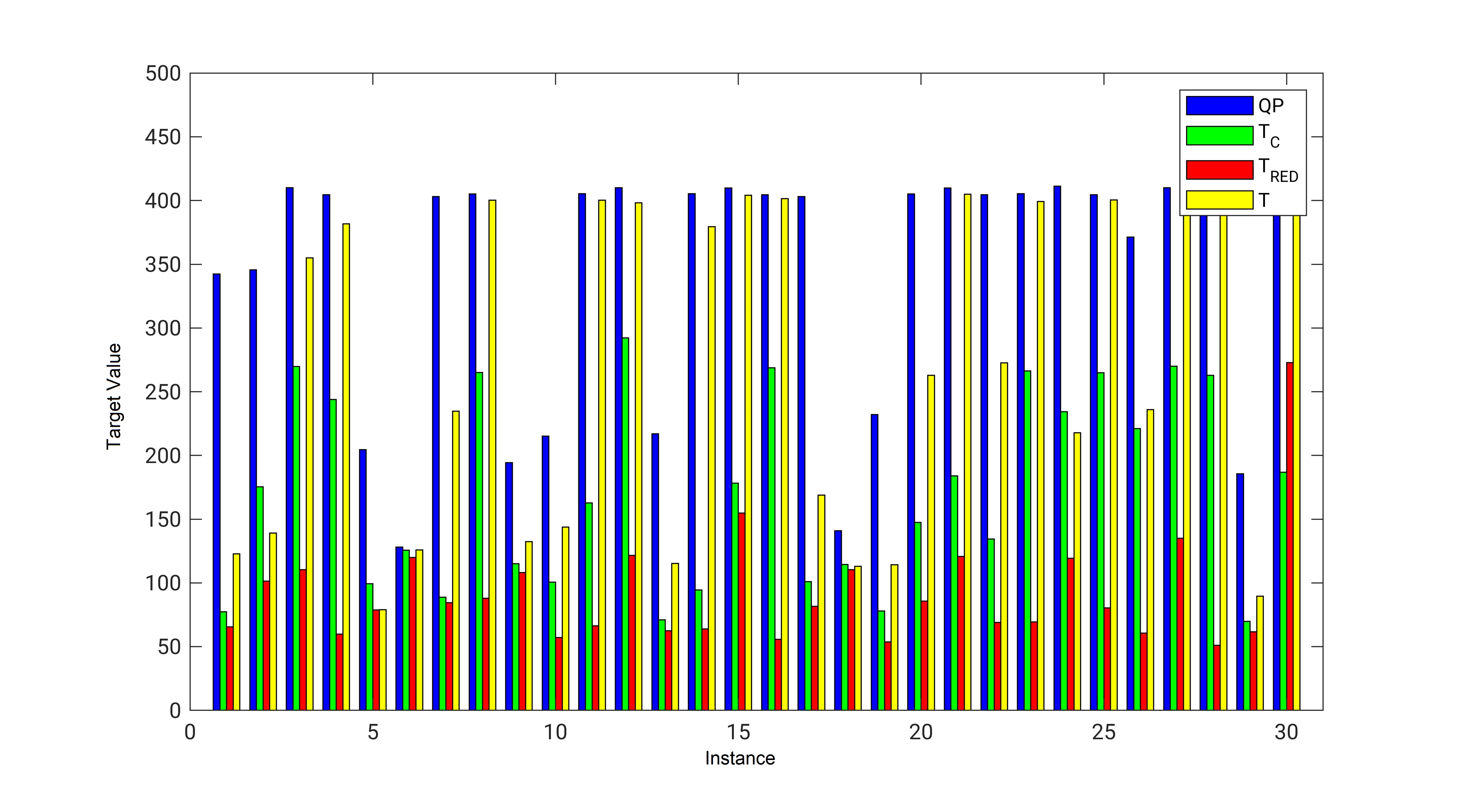
Figure 2: Target value $f(x)+\left\|x\right\|_{0}$ for portfolio selection with dimension $n=400$

In every instance we were able to improve on the solution QP, given by the $quadprog$-approach, with any of the solutions obtained by $T,T_{red}$ and $T_{C}$. Almost always, $T_{red}$ led to the best results followed by $T_{C}$ and finally $T$. However, $T_{red}$ as well as $T$ have a much higher iteration count than anticipated for a Newton-type method, which could be caused by the difficult structure of the constraints $x\circ y=0$ and $x\circ(1-\gamma\circ x/\rho)=0$, and the lack of a good initial guess $x^{0}$. Only $T_{C}$, where complementarity between $x$ and $y$ was handled by $\phi_{FB}$, delivered a sufficiently low iteration count.

7.3 Compressive Sensing

In its essence, compressive sensing deals with reconstructing an $n$-dimensional vector $\overline{x}$ encoded by some sensing-matrix $A\in\mathbb{R}^{m\times n}$ with $m\ll n$ into a signal $A\overline{x}=b$ of much lower dimension. Assuming that the original signal $\overline{x}$ was sparse sparse leads to the following formulation for compressive sensing

$$\min_{x}\ \left\|x\right\|_{0}\quad\text{s.t.}\quad Ax=b,$$ (33)

which was studied by Tao and Candès [6]. Problem (33) can be seen as an instance of SPO with $f\equiv 0$. Since we need some second order information for our local Newton-type methods, instead of the noise-free problem (33) we are more interested in the problem

$$\min_{x}\ \left\|x\right\|_{0}\quad\text{s.t.}\quad\left\|Ax-\overline{b}\right\|_{2}\leq\delta,$$

with some tolerance $\delta>0$. This problem is motivated by the assumption that the received signal is $\overline{b}=b+r$ with some noise $r$. However, this formulation requires that the noise level $\delta$ is known at least approximately. To avoid this problem, a penalty formulation

$$\min_{x}\ \frac{1}{2}\left\|Ax-\overline{b}\right\|^{2}_{2}+\rho\left\|x\right\|_{0}$$ (34)

as seen in [31] is often considered instead. Replacing the $\ell_{0}$-norm with the convex, sparsity inducing $\ell_{1}$-norm results in the basis persuit denoising problem, presented as in [8]:

$$\min_{x}\ \frac{1}{2}\left\|Ax-\overline{b}\right\|^{2}_{2}+\rho\left\|x\right\|_{1}.$$ (35)

In our numerical test, we compute an initial point $x^{0}$ by solving the $\ell_{1}$-surrogate problem (35) and then use $x^{0}$ together with the three Newton-type methods to solve (34).

We set up our examples as in [33]: Let $SA\in\mathbb{R}^{(m+p)\times n}$ be some sensing-matrix and $\overline{x}\in\mathbb{R}^{n}$ be some sparse vector. We set:

$$Sb:=SA\cdot\overline{x},$$

and split $SA$ and $Sb$ into:

$$SA=\begin{pmatrix}A\\ C\end{pmatrix},\quad A\in\mathbb{R}^{m\times n},C\in\mathbb{R}^{p\times n},\quad Sb=\begin{pmatrix}b\\ d\end{pmatrix},\quad b\in\mathbb{R}^{m},d\in\mathbb{R}^{p}.$$

We then consider the following problem

$$\min_{x}\ F_{\rho}(x):=\frac{1}{2}\left\|Ax-b\right\|_{2}^{2}+\rho\left\|x\right\|_{0}\quad\text{s.t.}\quad Cx=d,$$ (36)

where the linear constraints $Cx=d$ can be considered as noise-free information and exclude $x=0$ from the feasible set. The dimensions were set to $n=512,m=128$ and $p=8$, the sparsity of $\overline{x}$ was chosen as $s=\left\|\overline{x}\right\|_{0}=32$. The sensing-matrix $SA$ was initialized as a Gauß-matrix as in [32], such that:

$$SA_{j}\sim\mathscr{N}(0,E_{p+m}/(p+m)),\quad\forall j=1,...,n.$$

Closely following [33], we initialized the components of (36) as

$$\bar{x}=\texttt{zeros}(n,1), \Gamma=\texttt{randperm}(n), \bar{x}(\Gamma(1:s))=\texttt{randn}(s,1), Sb=SA\bar{x},$$

$$J=\texttt{randperm}(p+m), J_{1}=J(1:m), J_{2}=J(m+1:\textit{end}),$$

$$A=SA(J_{1}), b=Sb(J_{1}), C=SA(J_{2}), d=Sb(J_{2}).$$

To obtain an initial guess $x^{0}$, we considered the $\ell_{1}$-problem (35) as a quadratic program and applied MATLAB’s quadprog as seen in [17], which required the split $x=x_{+}-x_{-}$ with $x_{+},x_{-}\geq 0$. From the solution $(x_{+}^{0},x_{-}^{0})$ we could recover $x^{0}=x_{+}^{0}-x_{-}^{0}$. Note that in order to invoke the operator $T_{C}$, we now have to split $x$ into positive and negative part, because otherwise we do not have any nonnegativity constraints. For $T_{C}$ we thus used $(x_{+}^{0},x_{-}^{0})$ as is to initialize the algorithm. Unfortunately, this split leads to a much higher computational cost for $T_{C}$, since in every Newton-step a system of $6n+m$ equations had to be solved.

This time we chose a discrete set $\{0.1,0.5,1,2,3,4,5\}$ of values for $\rho$ and ran $100$ test examples for each of those values. We were faced with some unsuccessful runs regarding $T_{C}$, where the algorithm failed to converge in 5.6% of all tests, since either the iteration number exceeded the maximum of $100$ steps or we had to terminate early, as the error in the Newton-step with respect to the $\ell_{2}$-norm went past the safety threshold of $100$. For all values of $\rho$, the resulting average value $f(x)+\rho\left\|x\right\|_{0}$ of all successful runs is shown in Figure 3. Again, we observe a significant improvement of the objective function value for all operators $T,T_{red},T_{C}$, but now with less pronounced differences between the three operators.

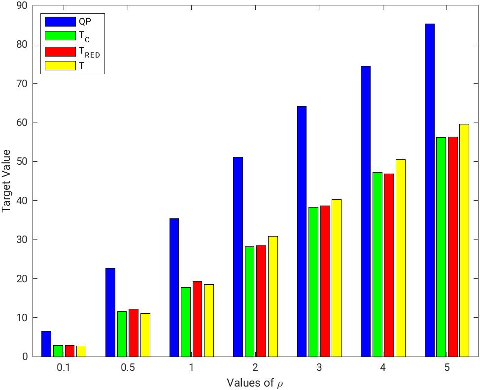
Figure 3: Average target value of $f(x)+\rho\left\|x\right\|_{0}$ for successful compressive sensing runs

7.4 Logistic Regression

Consider the following sparse optimization problem

$$\min_{w}\ \sum_{i=1}^{m}\log(1+\exp(-y_{i}\cdot w^{T}x_{i}))+\rho\left\|w\right\|_{0},$$ (37)

which we refer to as the penalized maximum log-likelihood function. This estimator is applied to match a sigmoid-function to a set of measurements $x_{1},...,x_{m}$ and corresponding Bernoulli-variables $y_{1},...,y_{n}\in\{-1,1\}^{m}$, where additionally sparsity is promoted in the parameters $w_{i}$. Replacing $\left\|\cdot\right\|_{0}$ by $\left\|\cdot\right\|_{1}$ in (37), we obtain a convex composite optimization problem, which can be tackled by FISTA or proximal BFGS methods, compare [23].

In our numerical test, we consider the problem gisette from the NIPS 2003 feature selection challenge, which was acquired from the LIBSVM-website. The classification problem is high-dimensional $(n=5000,m=6000)$ and was scaled to $[-1,1]$. Recall that applying either of the Newton-type methods with $T_{C},T$ or $T_{red}$ to the gisette problem leads to a drastic increase in the dimensionality (in the case of $T_{C}$: $n=30000$). Computation was therefore outsourced to a faster PC and handled in Python.

We computed an initial point $x^{0}$ by solving the $\ell_{1}$-surrogate problem to (37) with FISTA. Running the three Newton-type methods with this initial point then lead to the results in Figure 4. As one can see, all three of the operators lead to an improved sparsity $\|x\|_{0}$ and an improved function value $f(x)+\|x\|_{0}$, meaning a better solution of the original problem (37).

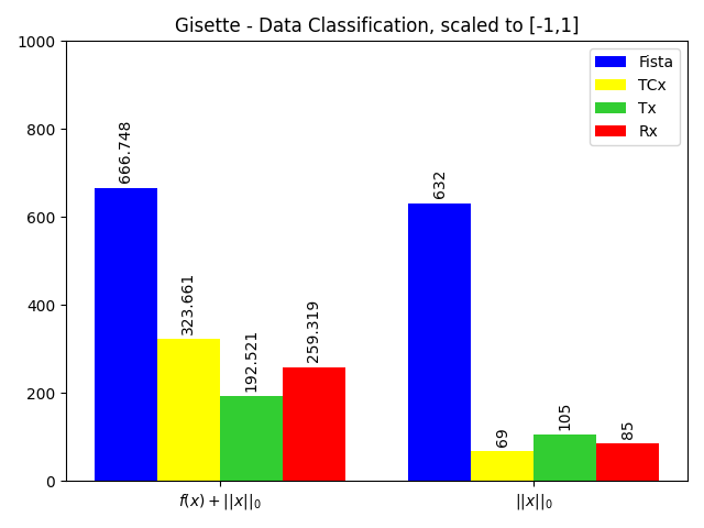
Figure 4: Comparison of target value $f(x)+\|x\|_{0}$ and sparsity $\|x\|_{0}$ for logistic regression

8 Final Remarks

The aim of this paper was mainly to lay the theoretical foundation fpr two reformulations of the highly difficult sparse optimization problem SPO. In particular, it was shown that we get full equivalence of problem SPO with these two reformulations in terms of global and local minima. Moreover, the corresponding stationary conditions also coincide and corresponding second-order conditions are closely related. These results can be used to develop and investigate Lagrange-Newton-type methods for the numerical solution of problem SPO and the numerical results indicate that one can use these methods in order to get significant improvements of solutions obtained by some other techniques.

The Lagrange-Newton-type methods, of course, are local in nature, but result quite naturally as a direct consequence of our theoretical considerations. Our future research, however, will concentrate on the development of globally convergent methods based on our reformulations. Some preliminary results in this direction can already be found in [29].

References

- [1] A. Beck. First-Order Methods in Optimization. SIAM, 2017.
- [2] R. Ben Mhenni, S. Bourguignon, and J. Ninin. Global optimization for sparse solution of least squares problems. Optimization Methods and Software, pages 1–30, 2021.
- [3] D. Bertsimas and B. Van Parys. Sparse high-dimensional regression: Exact scalable algorithms and phase transitions. The Annals of Statistics, 48(1):300–323, 2020.
- [4] J. F. Bonnans and A. Shapiro. Perturbation Analysis of Optimization Problems. Springer New York, 2000.
- [5] O. P. Burdakov, C. Kanzow, and A. Schwartz. Mathematical programs with cardinality constraints: reformulation by complementarity-type conditions and a regularization method. SIAM Journal on Optimization, 26(1):397–425, 2016.
- [6] E. Candes and T. Tao. Decoding by linear programming. IEEE Transactions on Information Theory, 51(12):4203–4215, 2005.
- [7] M. Červinka, C. Kanzow, and A. Schwartz. Constraint qualifications and optimality conditions for optimization problems with cardinality constraints. Mathematical Programming, 160(1):353–377, 2016.
- [8] S. S. Chen, D. L. Donoho, and M. A. Saunders. Atomic decomposition by basis pursuit. SIAM Journal on Scientific Computing, 20(1):33–61, 1998.
- [9] X. Chen, L. Guo, Z. Lu, and J. J. Ye. An augmented Lagrangian method for non-Lipschitz nonconvex programming. SIAM Journal on Numerical Analysis, 55(1):168–193, 2017.
- [10] F. H. Clarke. Optimization and Nonsmooth Analysis. SIAM, 1990.
- [11] T. De Luca, F. Facchinei, and C. Kanzow. A semismooth equation approach to the solution of nonlinear complementarity problems. Mathematical Programming, 75:407–439, 1996.
- [12] A. De Marchi, X. Jia, C. Kanzow, and P. Mehlitz. Constrained structured optimization and augmented Lagrangian proximal methods. Technical report, Institute of Mathematics, University of Würzburg, April 2022.
- [13] F. Facchinei, A. Fischer, and C. Kanzow. Regularity properties of a semismooth reformulation of variational inequalities. SIAM Journal on Optimization, 8(3):850–869, 1998.
- [14] F. Facchinei and J.-S. Pang. Finite-Dimensional Variational Inequalities and Complementarity Problems. Springer New York, 2004.
- [15] M. Feng, J. E. Mitchell, J.-S. Pang, X. Shen, and A. Wächter. Complementarity formulations of -norm optimization problems. Pacific Journal of Optimization, 14(2):273 – 305, 2018.
- [16] A. Fischer. A special Newton-type optimization method. Optimization, 24(3-4):269–284, 1992.
- [17] B. R. Gaines, J. Kim, and H. Zhou. Algorithms for fitting the constrained lasso. Journal of Computational and Graphical Statistics, 27(4):861–871, Aug. 2018.
- [18] D. Ghilli and K. Kunisch. A monotone scheme for sparsity optimization in with . IFAC-PapersOnLine, 50(1):494–499, 2017.
- [19] J.-y. Gotoh, A. Takeda, and K. Tono. DC formulations and algorithms for sparse optimization problems. Mathematical Programming, 169(1):141–176, 2018.
- [20] T. Hoheisel and C. Kanzow. Stationary conditions for mathematical programs with vanishing constraints using weak constraint qualifications. Journal of Mathematical Analysis and Applications, 337(1):292–310, 2008.
- [21] T. Hoheisel, C. Kanzow, and A. Schwartz. Theoretical and numerical comparison of relaxation methods for mathematical programs with complementarity constraints. Mathematical Programming, 137(1):257–288, 2013.
- [22] H. A. Le Thi, T. Pham Dinh, H. M. Le, and X. T. Vo. DC approximation approaches for sparse optimization. Technical report, 2014.
- [23] J. D. Lee, Y. Sun, and M. A. Saunders. Proximal Newton-type methods for minimizing composite functions. SIAM Journal on Optimization, 24(3):1420–1443, jan 2014.
- [24] Z. Lu and Y. Zhang. Penalty decomposition methods for -norm minimization. Technical report, 2012.
- [25] H. Markowitz. Portfolio selection. The Journal of Finance, 7(1):77–91, Mar. 1952.
- [26] P. Mehlitz. Stationarity conditions and constraint qualifications for mathematical programs with switching constraints. Mathematical Programming, 181(1):149–186, 2020.
- [27] L. Qi. Convergence analysis of some algorithms for solving nonsmooth equations. Mathematics of Operations Research, 18(1):227–244, 1993.
- [28] L. Qi and J. Sun. A nonsmooth version of Newton’s method. Mathematical programming, 58(1):353–367, 1993.
- [29] A. B. Raharja. Optimisation Problems with Sparsity Terms: Theory and Algorithms. Phd Thesis, Julius-Maximilians-Universität Würzburg, 2020.
- [30] A. M. Tillmann, D. Bienstock, A. Lodi, and A. Schwartz. Cardinality minimization, constraints, and regularization: A survey. Technical report, 2021.
- [31] L. Wang, J. Wang, J. Xiang, and H. Yue. A re-weighted smoothed -norm regularized sparse reconstructed algorithm for linear inverse problems. Journal of Physics Communications, 3(7):075004, July 2019.
- [32] P. Yin, Y. Lou, Q. He, and J. Xin. Minimization of for compressed sensing. SIAM Journal on Scientific Computing, 37(1):A536–A563, Jan. 2015.
- [33] C. Zhao, N. Xiu, H. Qi, and Z. Luo. A Lagrange-Newton algorithm for sparse nonlinear programming. Mathematical Programming, pages 1–26, 2021.