A Bayesian Convolutional Neural Network-based Generalized Linear Model

Abstract

Convolutional neural networks (CNNs) provide flexible function approximations for a wide variety of applications when the input variables are in the form of images or spatial data. Although CNNs often outperform traditional statistical models in prediction accuracy, statistical inference, such as estimating the effects of covariates and quantifying the prediction uncertainty, is not trivial due to the highly complicated model structure and overparameterization. To address this challenge, we propose a new Bayes approach by embedding CNNs within the generalized linear model (GLM) framework. We use extracted nodes from the last hidden layer of CNN with Monte Carlo dropout as informative covariates in GLM. This improves accuracy in prediction and regression coefficient inference, allowing for the interpretation of coefficient and uncertainty quantification. By fitting ensemble GLMs across multiple realizations from Monte Carlo dropout, we can fully account for uncertainties in model estimation. We apply our methods to simulated and real data examples, including non-Gaussian spatial data, brain tumor image data, and fMRI data. The algorithm can be broadly applicable to image regressions or correlated data analysis by enabling accurate Bayesian inference quickly.

1 Introduction

With recent advances in data collection technologies, it is increasingly common to have images as a part of collected data. For instance, in clinical trials, we can collect both fMRI images and clinical information from the same group of patients. However, it is challenging to analyze such data because variables represent different forms; we have both matrix (or tensor) images and vector covariates. The traditional statistical approaches face inferential issues when dealing with input variables in the form of images due to the high dimensionality and multicollinearity issues. Convolutional neural networks (CNN) (cf. Krizhevsky et al., 2012; He et al., 2016) are popular approaches for image processing without facing inferential challenges. However, CNNs cannot quantify the prediction uncertainty for the response variable and the estimation uncertainty for the covariates, which are often of primary interest in statistical inference. Furthermore, the complex structure of CNN can lead to nonconvex optimization (Ge et al., 2015; Kleinberg et al., 2018; Daneshmand et al., 2018; Alzubaidi et al., 2021), which cannot guarantee the convergence of weight parameters. In this manuscript, we propose a computationally efficient Bayesian approach by embedding CNNs within the generalized linear model (GLM). Our method can take advantage of both statistical models and advanced neural networks. We observe that our two-stage approach can provide a more accurate parameter estimate compared to the standard CNN.

There is a growing literature on Bayesian deep learning methods (cf. Neal, 2012; Blundell et al., 2015) to quantify the uncertainty by regarding weight parameters in deep neural networks (DNN) as random variables. With an appropriate choice of priors, we have posterior distributions for the standard Bayesian inference. Furthermore, Bayesian alternatives can be robust for a small sample size compared to the standard DNN (Gal and Ghahramani, 2016a, b). Despite its apparent advantages, however, Bayesian DNNs have been much less used than the classical one due to the difficulty in exploring the full posterior distributions. To circumvent the difficulty, variational Bayes (VB) methods have been proposed to approximate complex high-dimensional posteriors; examples include VB for feed-forward neural networks (Graves, 2011; Tran et al., 2020) and CNNs (Shridhar et al., 2019). Although VB can alleviate computational costs in Bayesian networks, to the best of our knowledge, no existing approach provides a general Bayesian framework to study image and vector type variables simultaneously. Furthermore, most previous works have focused on prediction uncertainty but not on estimation uncertainty of model parameters; interpretations of regression coefficients have not been studied much in the Bayesian deep learning context.

In this manuscript, we propose a Bayesian convolutional generalized linear model (BayesCGLM) that can study different types of variables simultaneously (e.g., regress a scalar response on vector covariates and array type images) and easily be implemented in various applications. A BayesCGLM consists of the following steps: (1) train Bayes CNN (Gal and Ghahramani, 2016a) with the correlated input (images or correlated variables) and output (response variable); (2) extract Monte Carlo samples of features from the last layer of the fitted Bayes CNN; and (3) fit a GLM by regressing a response variable on augmented covariates with the features obtained from each Monte Carlo sample. For each Monte Carlo sample of the feature, we fit an individual GLM and aggregate its posterior, which can be implemented in parallel. These steps allow us to fully account for uncertainties in the estimation procedure. We also study an often overlooked challenge in Bayesian deep learning: practical issues in obtaining credible intervals of parameters and assessing whether they provide nominal coverage.

In our method, we model Bayes CNN via a deep Gaussian process (Damianou and Lawrence, 2013), which is a nested Gaussian process. Gaussian process (Rasmussen, 2003) are widely used to represent complex function relationships due to their flexibility. Especially, Gal and Ghahramani (2016a, b) show that neural networks with dropout applied before the last layer is mathematically equivalent to the approximation of the posteriors of the deep Gaussian process (Damianou and Lawrence, 2013). This procedure is referred to as Bernoulli approximating variational distributions (Gal and Ghahramani, 2016a, b). We build upon their approach to sample features from the approximated posterior of the last layer in Bayes CNN. Training Bayes CNN with dropout approximation does not require additional computing costs compared to the frequentist one. There have been several recent proposals to extract features from the hidden layer of neural network models (Tran et al., 2020; Bhatnagar et al., 2022; Fong and Xu, 2021), and our method is motivated by them. The features can be regarded as reduced-dimensional summary statistics that measure complex non-linear relationships between the high-dimensional input and output; the dimension of the extracted features is much lower than that of the original input. We observe that CNN is especially useful for extracting information from correlated inputs such as images or spatial basis functions.

The outline of the remainder of this paper is as follows. In Section 2, we introduce a Bayesian DNN based on Gaussian process approximation and its estimation procedure. In Section 3, we propose a computationally efficient BayesCGLM and provide implementation details. In Section 4, we study the performance of BayesCGLM through simulated data examples. In Section 5, we apply BayesCGLM to several real-world data sets. We conclude with a discussion and summary in Section 6.

2 A Bayesian Deep Neural Network: Gaussian Process Approximation

In this section, we first give a brief review of Bayesian DNNs and their approximations to deep Gaussian processes. Let $\mathbf{D}=\{(\mathbf{x}_{n},\mathbf{y}_{n}),n=1,\cdots,N\}$ be the observed dataset with input $\mathbf{x}_{n}\in{\mathbb{R}}^{k_{0}}$ and response $\mathbf{y}_{n}\in{\mathbb{R}}^{d}$. A standard DNN is used to model the relationship between the input $\mathbf{x}_{n}$ and the output $\mathbf{o}_{n}\in{\mathbb{R}}^{d}$, which can be regarded as an expectation of $\mathbf{y}_{n}$ given $\mathbf{x}_{n}$, in terms of a statistical viewpoint. Suppose we consider a DNN model with $L$ layers, where the $l$th layer has $k_{l}$ nodes for $l=1,\cdots,L$. Then we can define the weight matrix $\mathbf{W}_{l}\in{\mathbb{R}}^{k_{l}\times k_{l-1}}$ that connects the $(l-1)$th layer to $l$th hidden layer and the bias vector $\mathbf{b}_{l}\in{\mathbb{R}}^{k_{l}}$. Then $\bm{\theta}=\{(\mathbf{W}_{l},\mathbf{b}_{l}),l=1,\cdots,L\}$ is a set of parameters in the neural network that belongs to a parameter space $\bm{\Theta}$.

To model complex data, the number of neural network parameters grows tremendously with the increasing number of layers and nodes. Such large networks are computationally intensive to use and can lead to overfitting issues. Dropout (Srivastava et al., 2014) has been suggested as a simple but effective strategy to address both problems. The term ”dropout” refers to randomly removing the connections from nodes during the training step of the network. While training, the model randomly chooses the units to drop out with some probability. The structure of neural networks with dropout is

$$\mathbf{o}_{n}=\sigma_{L}\Big{(}\mathbf{W}_{L}\sigma_{L-1}\Big{(}\mathbf{W}_{L-1}\cdots\sigma_{3}\Big{(}\mathbf{W}_{3}\sigma_{2}\Big{(}\mathbf{W}_{2}\sigma_{1}\Big{(}\mathbf{W}_{1}\mathbf{x}_{n}+\mathbf{b}_{1}\Big{)}\circ\mathbf{d}_{2}+\mathbf{b}_{2}\Big{)}\circ\mathbf{d}_{3}+\mathbf{b}_{3}\Big{)}\cdots\Big{)}\circ\mathbf{d}_{L-1}+\mathbf{b}_{L-1}\Big{)}\circ\mathbf{d}_{L}+\mathbf{b}_{L}\Big{)}$$ (1)

where $\sigma_{l}(\cdot)$ is an activation function; for instance, the rectified linear (ReLU) or the hyperbolic tangent function (TanH) can be used. Here $\mathbf{d}_{l}\in{\mathbb{R}}^{k_{l}},l=2,\cdots,L$, are dropout vectors whose components follow Bernoulli distribution with pre-specified success probability $p_{l}$ independently. The notation “$\circ$” indicates the elementwise multiplication of vectors. Although dropout can alleviate overfitting issues, quantifying uncertainties in predictions or parameter estimates remains challenging for the frequentist approach.

To address this, Bayesian alternatives (Friedman et al., 1997; Friedman and Koller, 2003; Chen and Pollino, 2012) have been proposed by considering probabilistic modeling of neural networks. The Bayesian approach considers an arbitrary function that is likely to generate data $\mathbf{D}$. Especially, a deep Gaussian process (deep GP) has been widely used to represent complex neural network structures for both supervised and unsupervised learning problems (Gal and Ghahramani, 2016b; Damianou and Lawrence, 2013). By modeling data generating mechanism as a deep GP, a hierarchical Bayesian neural network (Gal and Ghahramani, 2016b) can be constructed. For $l\geq 2$, let $\mathbf{f}_{n,l}=\mathbf{W}_{l}\bm{\phi}_{n,l-1}+\mathbf{b}_{l}\in{\mathbb{R}}^{k_{l}}$ be the linear feature which is a random variable in the Bayesian framework; we set independent normal priors for weight and bias parameters as $p(\mathbf{W}_{l})$ and $p(\mathbf{b}_{l})$ respectively. Then we can also define $\bm{\phi}_{n,l}=\sigma_{l}(\mathbf{f}_{n,l})\in{\mathbb{R}}^{k_{l}}$ as the nonlinear output feature from the $l$th layer after applying an activation function. For the first layer (i.e., $l=1$), we have $\mathbf{f}_{n,1}=\mathbf{W}_{1}\mathbf{x}_{n}+\mathbf{b}_{1}$. Then the deep GP can be written as

$$\begin{split}\mathbf{f}_{n,2}|\mathbf{x}_{n}&\sim N(0,\mathbf{\Sigma}_{nn,1})\\ \mathbf{f}_{n,3}|\mathbf{f}_{n,2}&\sim N(0,\mathbf{\Sigma}_{nn,2})\\ \vdots\\ \mathbf{f}_{n,L}|\mathbf{f}_{n,L-1}&\sim N(0,\mathbf{\Sigma}_{nn,L-1})\\ \mathbf{y}_{n}|\mathbf{f}_{n,L}&\sim p(\mathbf{y}_{n}|\mathbf{f}_{n,L}),\end{split}$$ (2)

where the covariance $\mathbf{\Sigma}_{nn,l}\in{\mathbb{R}}^{k_{l}\times k_{l}}$ is

$$\begin{split}\mathbf{\Sigma}_{nn,l}&=\int\int\sigma_{l}(\mathbf{W}_{l}\bm{\phi}_{n,l-1}+\mathbf{b}_{l})\sigma_{l}(\mathbf{W}_{l}\bm{\phi}_{n,l-1}+\mathbf{b}_{l})^{\top}p(\mathbf{W}_{l})p(\mathbf{b}_{l})d\mathbf{W}_{l}d\mathbf{b}_{l}.\end{split}$$ (3)

This implies that an arbitrary data generating function is modeled through a nested GP with the covariance of the extracted features from the previous hidden layer. Since the integral calculation in (3) is intractable, we can replace it with a finite covariance rank approximation in practice; with increasing $k_{l}$ (number of hidden nodes) the finite rank approximation becomes close to (3) (Gal and Ghahramani, 2016b). In (2), $\mathbf{y}_{n}$ is a response variable that has a distribution $p(\cdot)$ belonging to the exponential family with $g(E[\mathbf{y}_{n}|\bm{\phi}_{n,L-1}])=\mathbf{W}_{L}\bm{\phi}_{n,L-1}+\mathbf{b}_{L}$; here $g(\cdot)$ is a one-to-one continuously differential link function. Note that $g^{-1}(\cdot)$ can be regarded as $\sigma_{L}(\cdot)$ in (1) in terms of traditional DNN notation. To carry out Bayesian inference, we need to approximate the posterior distributions of deep GP.

However, Bayesian inference for deep GP is not straightforward to implement. With increasing hidden layers and nodes, the number of parameters $\bm{\theta}$ grows exponentially, resulting in a high-dimensional posterior distribution. Constructing Markov chain Monte Carlo (MCMC) samplers (Neal, 2012) is impractical due to the slow mixing of high-dimensional parameters and the complex sequential structure of the networks. Instead, variational approximation methods can be practical and computationally feasible for Bayesian inference (Bishop, 2006; Blei et al., 2017). Variational Bayes approximates the true $\pi(\bm{\theta}|\mathbf{D})$ via the approximate distribution (variational distribution) $q(\bm{\theta})$, which is a class of distribution that can be easily evaluated. Given a class of distributions, the optimal variational parameters are set by minimizing the Kullback–Leibler (KL) divergence between the variational distribution $q(\bm{\theta})$ and the true posterior $\pi(\bm{\theta}|\mathbf{D})$ where minimizing the KL divergence is equivalent to maximizing $\mbox{E}_{q}[{\log(\pi(\bm{\theta},\mathbf{D}))}]-\mbox{E}_{q}[\log q({\bm{\theta}})]$, the evidence lower bound (ELBO).

Gal and Ghahramani (2016b) shows that a deep neural network in (1) is mathematically equivalent to a variational approximation of deep Gaussian process (Damianou and Lawrence, 2013). That is the log ELBO of deep GP converges to the frequentist loss function of deep neural network with dropout layers. With the independent variational distribution $q(\bm{\theta}):=\prod_{l=1}^{L}q(\mathbf{W}_{l})q(\mathbf{b}_{l})$, the log ELBO of the deep GP is

$$\begin{split}\mathcal{L}_{\text{GP-VI}}:=\sum_{n=1}^{N}\int\cdots\int\prod_{l=1}^{L}q(\mathbf{W}_{l})q(\mathbf{b}_{l})\log p(\mathbf{y}_{n}|\mathbf{x}_{n},\{\mathbf{W}_{l},\mathbf{b}_{l}\}_{l=1}^{L})d\mathbf{W}_{1}\cdots d\mathbf{b}_{1}\cdots d\mathbf{W}_{L}d\mathbf{b}_{L}\\ -\text{KL}\Big{(}\prod_{l=1}^{L}q(\mathbf{W}_{l})q(\mathbf{b}_{l})\Big{|}\Big{|}p(\{\mathbf{W}_{l},\mathbf{b}_{l}\}_{l=1}^{L})\Big{)}.\end{split}$$ (4)

Here, $p(\mathbf{y}_{n}|\mathbf{x}_{n},\{\mathbf{W}_{l},\mathbf{b}_{l}\}_{l=1}^{L})$ is a conditional distribution, which can be obtained by integrating the deep GP (2) with respect to $\mathbf{f}_{n,l}$ for all $l$. Gal and Ghahramani (2016b) used a normal mixture distribution as a variational distribution for model parameters as follows:

$$\begin{split}q(\mathbf{W}_{l})&=\prod_{\forall i,j}q(w_{l,ij}),~{}~{}~{}q(\mathbf{b}_{l})=\prod_{\forall i}q(b_{l,i})\\ q(w_{l,ij})&=p_{l}N(\mu^{w}_{l,ij},\sigma^{2})+(1-p_{l})N(0,\sigma^{2})\\ q(b_{l,i})&=N(\mu^{b}_{l,i},\sigma^{2}),\end{split}$$ (5)

where $w_{l,ij}$ is the $i,j$th element of the weight matrix $\mathbf{W}_{l}\in{\mathbb{R}}^{k_{l}\times k_{l-1}}$ and $b_{l,i}$ is the $i$th element of the bias vector $\mathbf{b}_{l}\in{\mathbb{R}}^{k_{l}}$. For the weight parameters, $\mu^{w}_{l,ij}$ and $\sigma^{2}$ are variational parameters that control the mean and spread of the distributions, respectively. As the inclusion probability $p_{l}\in[0,1]$ becomes close to 0, $q({w}_{l,ij})$ becomes $N(0,\sigma^{2})$, indicating that it is likely to drop the weight parameters (i.e., $w_{l,ij}=0$). Similarly, the variational distribution for the bias parameters is modeled with normal distribution. Our goal is to obtain the variational parameters that maximize (4). Since the direct maximization of (4) is challenging due to the intractable integration, Gal and Ghahramani (2016b) replace it with approximation with distinct Monte Carlo samples for each observation as

$$\small\mathcal{L}_{\text{GP-MC}}:=\frac{1}{M}\sum_{m=1}^{M}\sum_{n=1}^{N}\log p(\mathbf{y}_{n}|\mathbf{x}_{n},\{\mathbf{W}_{l}^{(n,m)},\mathbf{b}_{l}^{(n,m)}\}_{l=1}^{L})-\text{KL}\Big{(}\prod_{l=1}^{L}q(\mathbf{W}_{l})q(\mathbf{b}_{l})\Big{|}\Big{|}\prod_{l=1}^{L}p(\mathbf{W}_{l})p(\mathbf{b}_{l})\Big{)},$$ (6)

where $\{\{\mathbf{W}_{l}^{(n,m)},\mathbf{b}_{l}^{(n,m)}\}_{l=1}^{L}\}_{m=1}^{M}$ is Monte Carlo samples from the variational distribution $\prod_{l=1}^{L}q(\mathbf{W}_{l})q(\mathbf{b}_{l})$ for $n$th observation. Note that the Monte Carlo samples are generated for each stochastic gradient descent updates, and the estimates from $\mathcal{L}_{\text{GP-MC}}$ would converge to those obtained from $\mathcal{L}_{\text{GP-VI}}$ (Bottou et al., 1991; Paisley et al., 2012; Rezende et al., 2014). In Section 4, we observe that even $M=1$ can provide reasonable approximations though the results become accurate with increasing $M$. Furthermore, Gal and Ghahramani (2016b) shows that (6) converges to the frequentist loss function of a deep neural network with dropout layers when $\sigma$ in 5 becomes zero and $k_{l}$ becomes large. This implies that the frequentist neural network with dropout layers is mathematically equivalent to the approximation of the posteriors of deep GP. We provide details in the Web Appendix A of the Supporting Information. Given this result, we can quantify uncertainty in the Bayesian network without requiring additional costs compared to the frequentist network.

In many applications, prediction of unobserved responses is of great interest. Based on the variational distributions obtained from (6), (Gal and Ghahramani, 2016b) provide a Bayesian framework for predictions in deep neural networks, which is called Monte Carlo dropout. Consider an unobserved response $\mathbf{y}^{\ast}\in{\mathbb{R}}^{d}$ with an input $\mathbf{x}^{\ast}\in{\mathbb{R}}^{k_{0}}$. For given $\mathbf{x}^{\ast}$, we can obtain $\bm{\phi}^{\ast}_{l}\in{\mathbb{R}}^{k_{l}}$ from the posterior predictive distribution of the deep GP in (2).

Although Gal and Ghahramani (2016b) focuses on predicting response variable $\mathbf{y}^{*}$, this procedure allows us to construct informative and low-dimensional summary statistics for unobserved $\mathbf{x}^{\ast}$. Especially, we can sample an output feature vector $\bm{\phi}^{\ast}_{n,L-1}\in{\mathbb{R}}^{k_{L-1}}$ which summarizes the complex nonlinear dependence relationships between input and output variables up to the last layer of the neural network. In Section 3, we use these extracted features as additional covariates in the GLM framework.

3 Flexible Generalized Linear Models with Convolutional Neural Networks

We propose a Bayesian convolutional generalized linear model (BayesCGLM) based on two appealing methodologies: (1) CNN (Krizhevsky et al., 2012) have been widely used to utilize correlated predictors (or input variables) with spatial structures such as images or geospatial data. (2) GLM can study the relationship between covariates and non-Gaussian response by extending a linear regression framework. Let $\mathbf{X}=\{\mathbf{X}_{n}\}_{n=1}^{N}$ be the collection of correlated input (i.e., each $\mathbf{X}_{n}$ is a matrix or tensor) and $\mathbf{Y}=\{\mathbf{y}_{n}\}_{n=1}^{N}$ be the corresponding output. We also let $\mathbf{Z}=\{\mathbf{z}_{n}\}_{n=1}^{N}$ be a collection of $p$-dimensional vector covariates. We use CNN to extract features from $\mathbf{X}_{n}$ and employ it in a GLM with the covariates $\mathbf{z}_{n}$ to predict $\mathbf{y}_{n}$. The uncertainties in estimating the features are quantified using Monte Carlo dropout. Now let $\bm{\Phi}^{(m)}=\{\bm{\phi}^{(m)\ast}_{n,L-1}\}_{n=1}^{N}\in{\mathbb{R}}^{N\times k_{L-1}}$ be the extracted features, which is the last hidden layer of CNN for $\mathbf{X}_{n}$, in the $m$th iteration of Monte Carlo dropout ($m=1,\cdots,M$). We begin with an outline of our framework:

Step 1. Train a Bayes CNN with the correlated data $\mathbf{X}$ (images or spatial variables) and covariate $\mathbf{Z}$ as input and $\mathbf{Y}$ as output. Here, the covariates $\mathbf{Z}$ are concatenated right after the last hidden layer.
Step 2. Using Monte Carlo dropout, extract features $\bm{\Phi}^{(m)}$ from the last hidden layer of the trained Bayes CNN for $m=1,\cdots M$.
Step 3. Fit GLMs by regressing $\mathbf{Y}$ on $[\mathbf{Z},\bm{\Phi}^{(m)}]$ for $m=1,\cdots,M$ in parallel. Posteriors from different $m$ (the “$m$th feature-posterior”) are aggregated to construct an ensemble-posterior distribution.

A graphical description of BayesCGLM is presented in Figure 1. We provide the details in the following subsections.

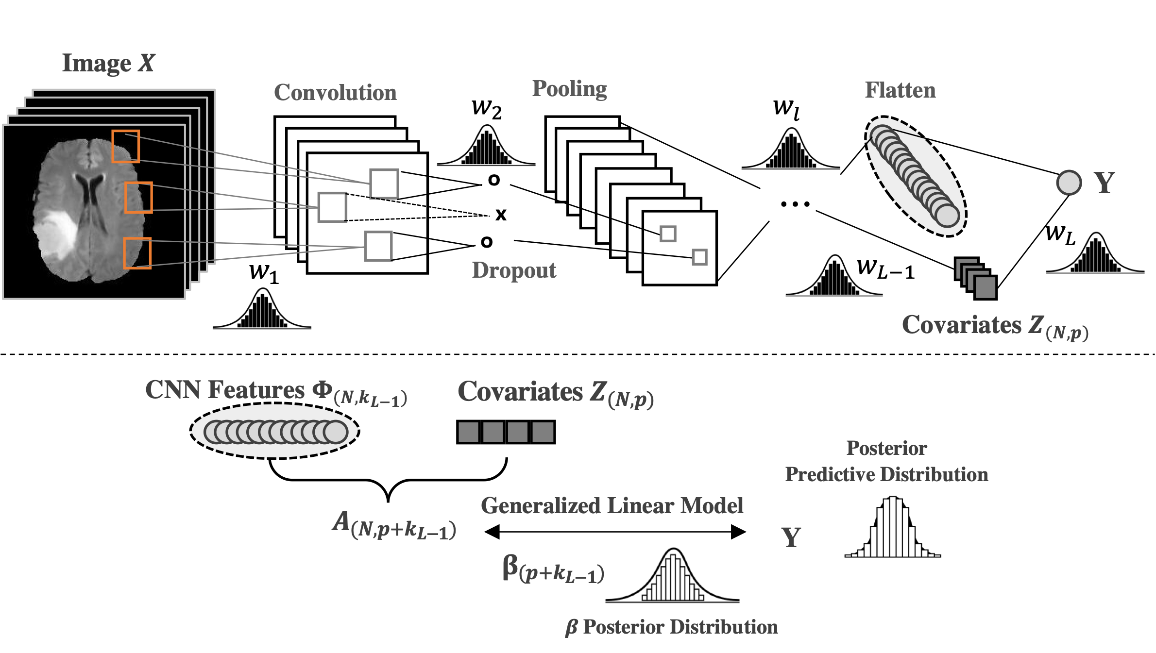
Figure 1: Illustration for the BayesCGLM.

3.1 Bayesian Convolutional Neural Network

As a variant of deep neural networks, convolutional neural networks (CNN) have been widely used in computer vision and image classification Krizhevsky et al. (2012); Shridhar et al. (2019). CNN can effectively extract important features of images or correlated datasets with non-linear dependencies. A Bayesian perspective, which regards weight parameters as random variables, can be useful because it enables uncertainty quantification in a straightforward manner through posterior densities. Especially, Gal and Ghahramani (2016a) proposes an efficient Bayesian alternative by regarding weight parameters in CNN’s kernels as random variables. By extending a result in Gal and Ghahramani (2016b), Gal and Ghahramani (2016a) shows that applying dropout after every convolution layer can approximate intractable posterior distribution of deep GP.

Let $\mathbf{X}_{n}\in{\mathbb{R}}^{M_{0}\times R_{0}\times C_{0}}$ be an input with $M_{0}$ height, $R_{0}$ width, and $C_{0}$ channels. For example, $M_{0}$ and $R_{0}$ are determined based on the resolution of images and $C_{0}=3$ for color images ($C_{0}=1$ for black and white images). There are three types of layers in CNN: the convolution, pooling, and fully coresulting innnected layers. Convolutional layers move kernels (filters) on the input image and extract information, resulting in a “feature map”. Each cell in the feature map is obtained from element-wise multiplication between the scanned input image and the filter matrix. The weight values in filter matrices are parameters to be estimated in CNN. The higher the output values, the more the corresponding portion of the image has high signals on the feature. This can account for spatial structures in input data; we can extract the important neighborhood features from the input by shifting the kernels over all pixel locations with a certain step size (stride) (Ravì et al., 2016). Then the pooling layers are applied to downsample the feature maps. The convolution and pooling layers are applied repeatedly to reduce the dimension of an input image. Then the extracted features from the convolution/pooling layers are flattened and connected to the output layer through a fully connected layer, which can learn non-linear relationships between the features and the output.

Consider a CNN with $L$ layers, where the last two are fully connected and output layers; we have convolutional operations up to $(L-2)$th layers. For the $l$th convolution layer, there are $C_{l}$ number of kernels $\mathbf{K}_{l,c}\in{\mathbb{R}}^{H_{l}\times D_{l}\times C_{l-1}}$ with $H_{l}$ height, $D_{l}$ width, and $C_{l-1}$ channels for $c=1,\cdots,C_{l}$. Note the dimension of channel is determined by the number of kernels in the previous convolution layer. After applying the $l$th convolution layer, the $(m,r)$th element of the feature matrix $\bm{\eta}_{n,(l,c)}\in{\mathbb{R}}^{M_{l}\times R_{l}}$ becomes

$$[\bm{\eta}_{n,(l,c)}]_{m,r}=\sigma\Big{(}\sum_{i=1}^{H_{l}}\sum_{j=1}^{D_{l}}\sum_{k=1}^{C_{l-1}}([\mathbf{K}_{l,c}]_{i,j,k}[\bm{\eta}_{n,(l-1,c)}]_{m+i-1,r+j-1,k})+b_{l,c}\Big{)},$$ (7)

where $b_{l,c}$ is the bias parameter. For the first convolution layer, $\bm{\eta}_{n,(l-1,c)}$ is replaced with an input image $\mathbf{X}_{n}$. (i.e., $\bm{\eta}_{n,(0,c)}=\mathbf{X}_{n}$). For computational efficiency and stability, ReLU functions are widely used as activation functions $\sigma(\cdot)$. By shifting kernels, the convolution layer can capture neighborhood information, and the neighborhood structure is determined by the size of the kernels.

Gal and Ghahramani (2016a) points out that extracting the features from the convolution process is equivalent to matrix multiplication in standard DNN (Figure 2). Without loss of generality, consider we have a single feature matrix $\bm{\eta}_{n,(l,1)}\in{\mathbb{R}}^{M_{l}\times R_{l}}$ with a kernel $\mathbf{K}_{l,1}\in{\mathbb{R}}^{H_{l}\times D_{l}}$ (i.e., $c=1$). As described in Figure 2, we can rearrange the $(l-1)$th input $\bm{\eta}_{n,(l-1,1)}$ as $\tilde{\bm{\eta}}_{n,(l-1,1)}\in{\mathbb{R}}^{M_{l}R_{l}\times H_{l}D_{l}}$ by vectorizing the $H_{l}\times D_{l}$ dimensional features from $\bm{\eta}_{n,(l-1,1)}$. Similarly, we can vectorize the kernel $\mathbf{K}_{l,1}$ and represent it as a weight matrix $\tilde{\mathbf{W}}_{l,1}\in{\mathbb{R}}^{H_{l}D_{l}}$. Then, we can perform matrix multiplication $\tilde{\bm{\eta}}_{n,(l-1,1)}\tilde{\mathbf{W}}_{l,1}\in{\mathbb{R}}^{M_{l}R_{l}}$ and rearrange it to obtain a matrix $\bm{\eta}_{n,(l,1)}\in{\mathbb{R}}^{M_{l}\times R_{l}}$, which is equivalent to output from the $l$th convolution layer. The above procedure can be generalized to the tensor input $\bm{\eta}_{n,l-1}=\{\bm{\eta}_{n,(l-1,c)}\}_{c=1}^{C_{l-1}}\in{\mathbb{R}}^{M_{l-1}\times R_{l-1}\times C_{l-1}}$ with $C_{l}$ number of kernels $\mathbf{K}_{l,c}\in{\mathbb{R}}^{H_{l}\times D_{l}\times C_{l-1}}$; therefore, the convolution process is mathematically equivalent to standard DNN. Similar to DNN, we can construct posterior distributions for weights and bias parameters. Then the posterior distributions are approximated through variational distributions in (5), which are normal mixtures. As described in Section 2, applying dropout after every convolution layer before pooling can approximate deep GP (Damianou and Lawrence, 2013).

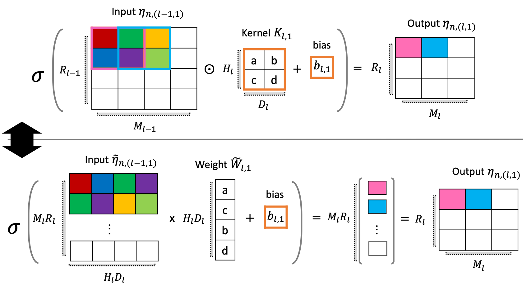
Figure 2: Illustration for the convolution operation. The convolution process is mathematically equivalent to the matrix product in standard DNN.

After the $L-2$th convolution layers, the extracted feature tensor $\bm{\eta}_{n,L-2}\in{\mathbb{R}}^{M_{L-2}\times R_{L-2}\times C_{L-2}}$ is flattened in the fully connected layer. By vectorizing $\bm{\eta}_{n,L-2}$, we can represent the feature tensor as a feature vector $\bm{\phi}_{n,L-2}=\operatorname{vec}(\bm{\eta}_{n,L-2})\in{\mathbb{R}}^{k_{L-2}}$, where $k_{L-2}=M_{L-2}R_{L-2}C_{L-2}$. Finally, we can extract a feature vector $\bm{\phi}_{n,L-1}\in{\mathbb{R}}^{k_{L-1}}$ from the fully connected layer; the collection of feature vectors $\bm{\Phi}=\{\bm{\phi}_{n,L-1}\}_{n=1}^{N}\in{\mathbb{R}}^{N\times k_{L-1}}$ summarizes high-dimensional input into a lower dimensional space.

3.2 Bayesian Convolutional Generalized Linear Model

We propose BayesCGLM by regressing $\mathbf{Y}$ on $\bm{\Phi}$ and additional covariates $\mathbf{Z}$. Here, we use $\bm{\Phi}$ as a basis design matrix that encapsulates information from high-dimensional and correlated input variables in $\mathbf{X}$. The proposed method can provide interpretation of the regression coefficients and quantify uncertainties in prediction and estimation. As the first step, we train Bayes CNN with the $\mathbf{X}$ and $\mathbf{Z}$ as input and $\mathbf{Y}$ as output. We concatenate the covariate $\mathbf{Z}$ right after the last hidden layer to model the effects of $\mathbf{X}$ on $\mathbf{Y}$ for a given fixed $\mathbf{Z}$. Compared to the traditional CNN, the training step does not require additional computational costs. Then we can extract the feature $\bm{\Phi}\in{\mathbb{R}}^{N\times k_{L-1}}$ from the last hidden layer. We can regard this feature as an informative summary statistic that can measure potentially non-linear effects of the input $\mathbf{X}$ on $\mathbf{Y}$. Since we place a posterior distribution over the kernels of the fitted CNN (Section 3.1), we can generate Monte Carlo samples of the features $\bm{\Phi}^{(m)}$, $m=1,\cdots,M$ from the variational distribution. To account for the uncertainties in estimating the features $\bm{\Phi}$, we use the entire Monte Carlo samples of the features rather than the point estimates of them. In Section 4, we demonstrate that this allows us to fully account for uncertainties in the feature extraction step through various simulated examples.

With the covariate matrix $\mathbf{Z}\in{\mathbb{R}}^{N\times p}$, we fit $M$ different GLMs by regressing $\mathbf{Y}$ on $\mathbf{A}^{(m)}=[\mathbf{Z},\bm{\Phi}^{(m)}]\in{\mathbb{R}}^{N\times(p+k_{L-1})}$. Then, our model is

$$\begin{split}g(E[\mathbf{Y}|\mathbf{Z},\bm{\Phi}^{(m)}])&=\mathbf{Z}\bm{\gamma}_{m}+\bm{\Phi}^{(m)}\bm{\delta}_{m}=\mathbf{A}^{(m)}\bm{\beta}_{m}\end{split}$$ (8)

where $\bm{\beta}_{m}=(\bm{\gamma}_{m}^{\top},\bm{\delta}_{m}^{\top})^{\top}\in{\mathbb{R}}^{p+k_{L-1}}$ is the corresponding regression coefficients and $g(\cdot)$ is a one-to-one continuously differential link function.

For each Monte Carlo sample $m$, we can fit individual GLM in parallel; we have $m=1,\cdots,M$ number of posterior distributions, and each of them can be called the “$m$th feature-posterior.” This step is heavily parallelizable, so computational walltimes tend to decrease with an increasing number of available cores. Then, we construct an aggregated distribution (the “ensemble-posterior”) through the mixture of feature posteriors. In the following section, we provide details about constructing the ensemble-posterior distribution. The fitting procedure of BayesCGLM is summarized in Algorithm 1.

Algorithm 1 BayesCGLM algorithm

Input: $\mathbf{X}$ (image or correlated input), $\mathbf{Y}$ (response), $\mathbf{Z}$ (scalar covariates)

Output: Posterior distribution of model parameters.

1:Fit Bayes CNN by using $\mathbf{X}$ and $\mathbf{Z}$ as input and $\mathbf{Y}$ as output. Then for each $m$

2:for $m=1,2,\ldots,M$ do

3:     Extract features $\bm{\Phi}^{(m)}$ from the last hidden layer.

4:     Fit GLM by regressing $\mathbf{Y}$ on $[\mathbf{Z},\bm{\Phi}^{(m)}]$ through the Laplace approximation

5:     Obtain the $m$th feature-posterior distribution of model parameter.

6:end for

7:Construct an ensemble-poseterior by aggregating $M$ feature-posteriors.

Since BayesCGLM in (8) can capture non-linear effects of $\mathbf{X}$ on $\mathbf{Y}$ through the extracted features $\bm{\Phi}$, we can improve prediction accuracies compared to the standard GLM. In general, inference for the regression coefficients $\bm{\gamma}$ is challenging for DNN. Although one can regard the weight parameters at the last hidden layer as $\bm{\gamma}$, we cannot obtain uncertainties of estimates. Note that even Bayes DNN (Gal and Ghahramani, 2016b) only provides point estimates of weight parameters, while they can quantify uncertainties in response prediction. On the other hand, our method directly provides the posterior distribution of $\bm{\gamma}$, which is useful for standard inference. In addition, the complex structure of DNN often leads to nonconvex optimization (Ge et al., 2015; Kleinberg et al., 2018; Daneshmand et al., 2018), resulting in inaccurate estimate of $\bm{\gamma}$. Stochastic gradient descent algorithm requires simultaneous updates of high-dimensional weight parameters. Instead, our two-stage approach can alleviate this issue by using extracted features $\bm{\Phi}$ as a fixed basis matrix in GLM.

Figure 3 illustrates the profile log-likelihood surfaces over $\bm{\gamma}$ based on a single replicate from our simulation studies in Section 4. Note that we use the same CNN structure to make the profile log-likelihood surfaces comparable. We observe that our two-stage approach provides more accurate estimates compared to BayesCNN. Since the stopping rule of the stochastic gradient descent algorithm is based on prediction accuracy (not based on convergence in parameter estimation), the convergence of individual weight parameters, including $\bm{\gamma}$ cannot be guaranteed. The problem gets further complicated by a large number of weight parameters that need to be simultaneously updated in CNN (Alzubaidi et al., 2021). On the other hand, BayesCGLM converts the complex optimization into simple nonparametric regression problems by utilizing the extracted features $\bm{\Phi}$ as a fixed basis function. This allows application of more accurate optimization algorithms based on convergence in parameter estimates. In Section 4, we repeat the simulation 300 times under different model configurations and show that BayesCGLM can recover the true $\bm{\gamma}$ values well, while estimates from Bayes DNN can be biased.

(a) The profile log-likelihood in BayesCNN

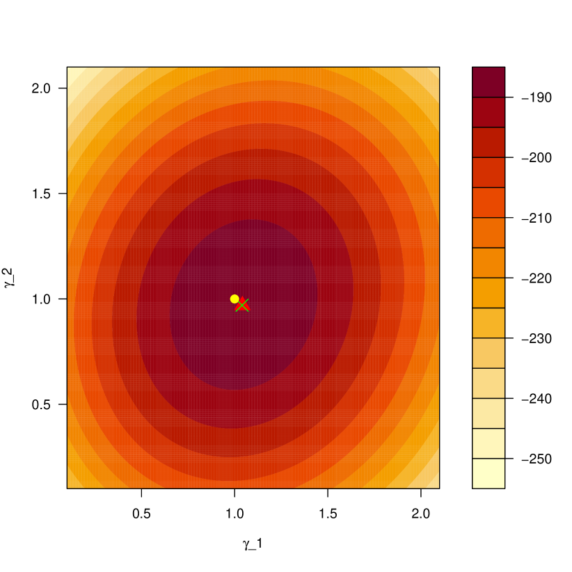
(b) The profile log-likelihood in BayeCGLM

Figure 3: The yellow circles show the true coefficient $\bm{\gamma}=(1,1)$, the green x-crosses indicate the maximum likelihood points, and the red triangles represent the estimates obtained from BayesCNN and BayesCGLM, respectively. BayesCGLM provides a closer estimate to the true $\bm{\gamma}$ than BayesCNN.

3.3 Bayesian Inference

Our framework requires Bayesian inference on ensemble GLMs in (8), i.e., fitting $M$ different GLM models in a Bayesian way. One may choose the standard MCMC algorithm, which can provide exact Bayesian inference. However, this may require a long run of the chain to guarantee a good mixing, resulting in excessive computational cost in our framework. To fit ensemble GLMs quickly, we use the Laplace approximation method (Tierney and Kadane, 1986). In our preliminary studies, we observe that there are little benefits from the more exact method; for enough sample size, the Laplace approximation method provides reasonably accurate approximations to the posteriors within a much shorter time.

For each dropout realization $m$, we can obtain the maximum likelihood estimate (MLE) $\widehat{\bm{\beta}}_{m}$ of (8) using the iteratively reweighted least square algorithm, which can be implemented through statmodels function in Python. Then we can approximate the posterior of $\bm{\beta}_{m}$ through $\mathcal{N}(\widehat{\bm{\beta}}_{m},\widehat{\mathbf{B}}^{-1}_{m})$, where $\widehat{\mathbf{B}}_{m}\in{\mathbb{R}}^{(p+k_{L-1})\times(p+k_{L-1})}$ is the observed Fisher information matrix from the $m$th Monte Carlo samples. We can obtain such approximated posteriors for $m=1,\cdots,M$ from Monte Carlo dropout realizations. We can aggregate these feature-posteriors with the mixture distribution as

$$\widehat{\pi}(\bm{\beta}|\mathbf{D})=\sum_{m=1}^{M}\omega_{m}\varphi(\bm{\beta};\widehat{\bm{\beta}}_{m},\widehat{\mathbf{B}}^{-1}_{m})$$ (9)

where $\varphi(\bm{x};\bm{\mu},\bm{\Sigma})$ is a multivariate normal density with mean $\bm{\mu}$ and covariance $\bm{\Sigma}$. Here, we used the equal weight for $\omega_{m}$ across different Monte Carlo dropout realizations (i.e., $\omega_{m}=1/M$). Especially, we focus on describing inference for the posterior distribution of the regression coefficient $\bm{\gamma}$, which can quantify the impact of $\mathbf{Z}$ on $\mathbf{Y}$. Since we have an ensemble-posterior distribution (9), we can conduct standard Bayesian inference naturally.

Our Bayesian framework also quantifies uncertainties in predictions which is another advantages over existing neural networks. For unobserved response $\mathbf{Y}^{\ast}\in{\mathbb{R}}^{N_{cv}}$, we have $\mathbf{A}^{\ast}_{m}=[\mathbf{Z}^{\ast},\bm{\Phi}^{(m)}]\in{\mathbb{R}}^{N_{cv}\times(p+k_{L-1})}$ for $m=1,\cdots,M$. Then from (9), the distribution of the linear predictor is

$$\widehat{\pi}(\mathbf{A}^{\ast}\bm{\beta}|\mathbf{D})=\sum_{m=1}^{M}\omega_{m}\varphi(\mathbf{A}^{\ast}\bm{\beta};\mathbf{A}_{m}^{\ast}\widehat{\bm{\beta}}_{m},\mathbf{A}_{m}^{\ast}\widehat{\mathbf{B}}^{-1}_{m}\mathbf{A}^{\ast\top}_{m}).$$ (10)

From the linear predictor above, we can construct the posterior predictive distribution. For given a posterior mean $\widehat{\bm{\beta}}$ from (9), we can generate $\mathbf{Y}^{\ast}$ from the exponential family distribution with mean $\mathbf{A}^{\ast}\bm{\hat{\beta}}$. For example, when we have a Gaussian response we have $\mathbf{Y}^{\ast}\sim\mathcal{N}(\mathbf{A}^{\ast}\bm{\hat{\beta}},\hat{\sigma}^{2})$ where $\hat{\sigma}^{2}=\frac{\sum_{n=1}^{N}(\mathbf{A}^{\ast}\bm{\hat{\beta}}-\mathbf{Y})}{N}$ for the Gaussian response. For the count response, we can simulate $\mathbf{Y}^{\ast}$ from the Poisson distribution with intensity $\mathbf{A}^{\ast}\bm{\hat{\beta}}$.

4 Simulated Data Examples

In this section, we apply BayesCGLM to three different simulated examples, with a Gaussian response (described in the Web Appendix D), binary response (Section 4.1), and Poisson response (Section 4.2). We implement our approach in TensorFlow, an open-source platform for machine learning. Parallel computation is implemented through the multiprocessing library in Python. The computation times are based on 8 core AMD Radeon Pro 5500 XT processors. The configuration of the CNN structures and tuning details used in our experiments are provided in the Web Appendix B.1 of the Supporting Information.

We generated 1,000 lattice datasets as images, which have a spatially correlated structure given by the Gaussian process. The responses are created by the canonical link function $g^{-1}$ and the natural parameter $\bm{\lambda}=g^{-1}(\bm{\Phi}+\mathbf{Z}\bm{\gamma})$ with $\bm{\gamma}=(1,1)$. Here, $\bm{\Phi}$ indicates the vectorized local features of the images, $\mathbf{Z}$ represents covariates generated from a standard normal distribution, and $\bm{\gamma}$ are the true coefficients. To demonstrate the performance of our model, we compared it with two existing models: Bayesian CNN and GLM. The details of simulation experiments are described in the Web Appendix C of the Supporting Information.

4.1 Binary Case

We now describe the simulation study results when $\mathbf{Y}$ is in the form of binary response, i.e., $\mathbf{Y}\sim\text{Bernoulli}(\bm{\lambda})$. Figure 4 compares the true response and the estimated probabilities (for the response to be 1), which show a good agreement. We observe that the predicted probability shows higher values for the binary responses with the true value of 1. The area under the curve (AUC) from the receiver operating characteristic curve (ROC) is about 0.85, which is reasonably close to 1 (Figure 4(b)).

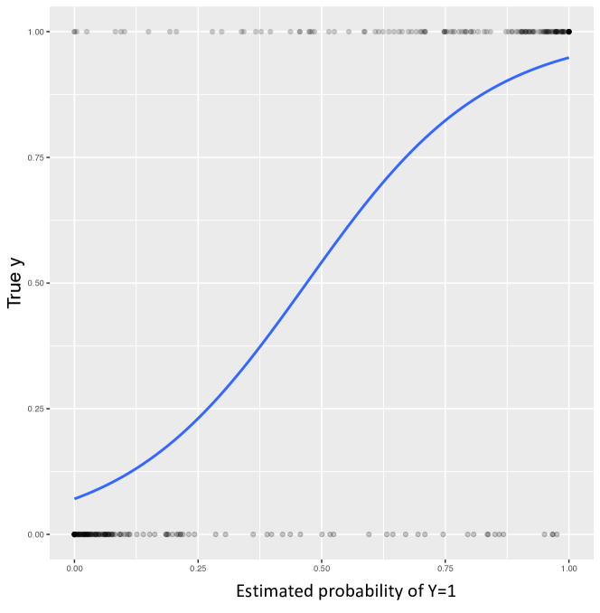
(a) Predicted probability surface

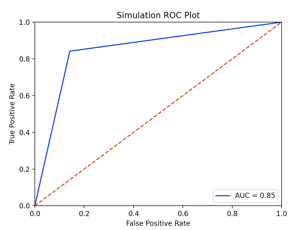
(b) ROC plot

Figure 4: (a) The scatter plot of estimated probability of $Y=1$ and true binary responses. Blue line indicates the estimated probability function. (b) The ROC curve for binary prediction. Blue line denotes AUC of the ROC curve.

In Table 1 we observe that parameter estimates from BayesCGLM are accurate, and the coverages are close to the 95% nominal rate even with a single Monte Carlo dropout ($M=1$). On the other hand, the estimates from Bayes CNN (Gal and Ghahramani, 2016a), and GLM are biased. Deep learning methods (BayesCGLM, Bayes CNN) show much better prediction performance than GLM because they can extract features from image observations.

Table 1: Inference results for the simulated binary datasets. For all methods, mean of $\bm{\gamma}$, estimation coverage, accuracy, recall, precision, and average computing time (sec) are calculated from 300 simulations. The numbers in the parentheses indicate standard deviations obtained from the repeated simulations.

	BayesCGLM(M$=300$)	BayesCGLM(M$=1$)	Bayes CNN	GLM
$\gamma_{1}$	1.029 (0.154)	1.030 (0.154)	0.848 (0.117)	0.389 (0.086)
Coverage	0.956	0.966	-	0
$\gamma_{2}$	1.030 (0.151)	1.024 (0.155)	0.851 (0.120)	0.388 (0.081)
Coverage	0.954	0.952	-	0
Accuracy	0.869 (0.019)	0.857 (0.022)	0.850 (0.022)	0.600 (0.028)
Recall	0.869 (0.031)	0.855 (0.033)	0.851 (0.036)	0.600(0.066)
Precision	0.868 (0.030)	0.858 (0.033)	0.863 (0.029)	0.602 (0.043)
Time	37.028	17.661	15.022	0.003

4.2 Poisson Case

We describe the simulation study results when $\mathbf{Y}$ is generated from the Poisson distribution, i.e., $\mathbf{Y}\sim\text{Poisson}(\bm{\lambda})$. Figure 5 shows that the true and predicted responses are well aligned for a simulated dataset except for some extreme values. We observe that HPD prediction intervals include the true count response well.

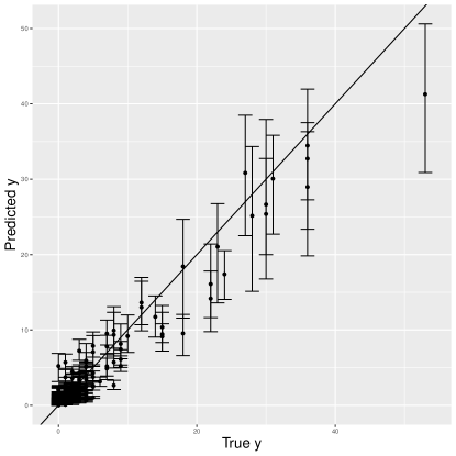
Figure 5: Comparison between the true and predicted Poisson responses from BayesCGLM. The vertical lines indicate 95% highest posterior density (HPD) from the predictive distribution.

Table 2 indicates that BayesCGLM shows comparable (or better) prediction performance compared to Bayes CNN while providing uncertainties of estimates. We observe that the coverage of the credible and prediction intervals becomes closer to the 95% nominal rate with the repeated Monte Carlo dropout sampling ($M=300$), compared to a single Monte Carlo dropout sampling ($M=1$). Compared to Bayes CNN, BayesCGLM with $M=300$ results in better point estimates for the parameters $\bm{\gamma}$ and point predictions for the response $\mathbf{Y}$. Compared to GLM, BayesCGLM with $M=300$ results in better empirical coverage for the credible intervals for $\bm{\gamma}$ as well as better prediction accuracy and empirical coverage for the prediction intervals for $\mathbf{Y}$.

Table 2: Inference results for the simulated Poisson datasets. For all methods, mean of $\bm{\gamma}$, estimation coverage, RMSPE, prediction coverage, and average computing time (min) are calculated from 300 simulations. The numbers in the parentheses indicate standard deviations obtained from the repeated simulations.

	BayesCGLM(M$=300$)	BayesCGLM(M$=1$)	Bayes CNN	GLM
$\gamma_{1}$	0.987 (0.027)	0.989 (0.031)	0.910 (0.106)	0.997 (0.058)
Coverage	0.936	0.862	-	0.542
$\gamma_{2}$	0.986 (0.026)	0.989 (0.031)	0.911 (0.101)	0.997 (0.059)
Coverage	0.958	0.868	-	0.550
RMSPE	2.305 (1.610)	2.687 (2.190)	2.737 (2.537)	4.364 (3.739)
Coverage	0.963	0.890	0.967	0.924
Time	22.73	15.285	13.753	0.004

5 Applications

We apply our method to three real data examples: (1) malaria incidence data, (2) brain tumor images, and (3) fMRI data for anxiety scores. We attached fMRI data for anxiety score result in the Web Appendix E of the Supporting Information. BayesCGLM shows comparable prediction with the standard Bayes CNN while enabling uncertainty quantification for regression coefficients. Details about the CNN structure are provided in the Web Appendix B.2 of the Supporting Information.

5.1 Malaria Cases in the African Great Lakes Region

Malaria is a parasitic disease that can lead to severe illnesses and even death. Predicting occurrences at unknown locations is of significant interest for effective control interventions. We compiled malaria incidence data from the Demographic and Health Surveys of 2015 (ICF, 2020). The dataset contains malaria incidence (counts) from 4,741 GPS clusters in nine contiguous countries in the African Great Lakes region. We use average annual rainfall, vegetation index of the region, and the proximity to water as spatial covariates. Under a spatial regression framework, Gopal et al. (2019) analyzes malaria incidence in Kenya using these environmental variables. In this study, we extend this approach to multiple countries in the African Great Lakes region. We use $N=3,500$ observations to fit the model and save $N_{\text{cv}}=1,241$ observations for cross-validation.

To create rectangular images out of irregularly shaped spatial data, we use a spatial basis function matrix as the correlated input $\mathbf{X}$ in Algorithm 1 (line 1). Specifically, we use thin plate splines basis defined as $\mathbf{X}_{j}(\mathbf{s})=||\mathbf{s}-\mathbf{u}_{j}||^{2}\log(||\mathbf{s}-\mathbf{u}_{j}||)$, where $s$ is an arbitrary spatial location and $\{\mathbf{u}_{j}\}_{j=1}^{239}$ is a set of knots placed regularly over the spatial domain. From this we can construct basis functions for each observation, resulting in $\mathbf{X}\in{\mathbb{R}}^{3,500\times 239}$ input design matrix. We first train Bayes CNN with input $\mathbf{X},\mathbf{Z}$ and the count response $\mathbf{Y}$ while applying Monte Carlo dropout, with a dropout probability of 0.2. We set the batch size and epochs as 10 and 500, respectively. We use ReLU and linear activation functions in the hidden layers and use the exponential activation function in the output layer to fit count response. From this, we extract a feature design matrix $\bm{\Phi}\in{\mathbb{R}}^{3,500\times 16}$ from the last layer of the fitted Bayes CNN. With covariate matrix $\mathbf{Z}\in{\mathbb{R}}^{3,500\times 3}$, we fit Poisson GLMs by regressing $\mathbf{Y}$ on $[\mathbf{Z},\bm{\Phi}^{(m)}]\in{\mathbb{R}}^{3,500\times 19}$ for each $m$; here, we have used $M=500$.

We compare our method with a spatial regression model using basis expansions (cf. Sengupta and Cressie, 2013; Lee and Park, 2022) as

$$g(E[\mathbf{Y}|\mathbf{Z},\mathbf{X}])=\mathbf{Z}\bm{\gamma}+\mathbf{X}\bm{\delta},$$

where $\mathbf{X}\in{\mathbb{R}}^{3,500\times 239}$ is the same thin plate basis matrix that we used in BayesCGLM. To fit a hierarchical spatial regression model, we use nimble (de Valpine et al., 2017), which is a convenient programming language for Bayesian inference. To guarantee convergence, an MCMC algorithm is run for 1,000,000 iterations with 500,000 discarded for burn-in. Furthermore, we also implement the Bayes CNN as in the simulated examples. Table 3 indicates that vegetation, water, and rainfall variables have positive relationships with malaria incidence in deep learning methods. BayesCGLM shows comparable prediction performance compared to Bayes CNN. Although Bayes CNN can provide prediction uncertainties, it cannot quantify uncertainties of the estimates. Although, we can obtain HPD intervals from spatial regression, it provides higher RMSPE and lower coverage than other deep learning methods.

Table 3: Inference results for the malaria dataset from different methods. For all methods, posterior mean of $\bm{\gamma}$, 95% HPD interval, RMSPE, prediction coverage, and computing time (min) are reported in the table.

	BayesCGLM(M=500)	Bayes CNN	Spatial Model
$\gamma_{1}$ (vegetation index)	0.099	0.103	0.115
	(0.092 0.107)	-	(0.111 0.118)
$\gamma_{2}$ (proximity to water)	0.074	0.058	-0.269
	(0.068 0.080)	-	(-0.272 -0.266)
$\gamma_{3}$ (rainfall)	0.036	0.027	-0.122
	(0.027 0.045)	-	(-0.126 -0.117)
RMSPE	27.438	28.462	42.393
Coverage	0.950	0.947	0.545
Time	57.518	30.580	41.285

Figure 6(a) shows that the true and predicted malaria incidence from BayesCGLM have similar spatial patterns. We observe the prediction standard errors are reasonably small across the entire spatial domain. Similar to the simulation studies, we illustrate the 95% HPD prediction intervals, which include the true count response well.

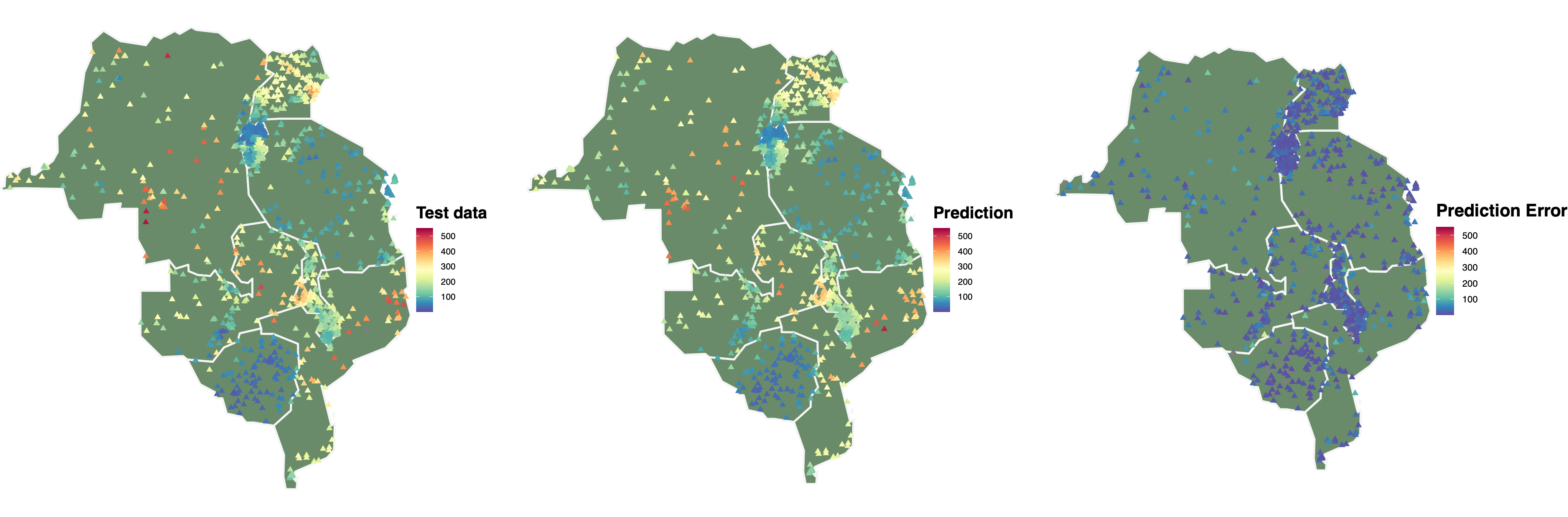
(a) Prediction map

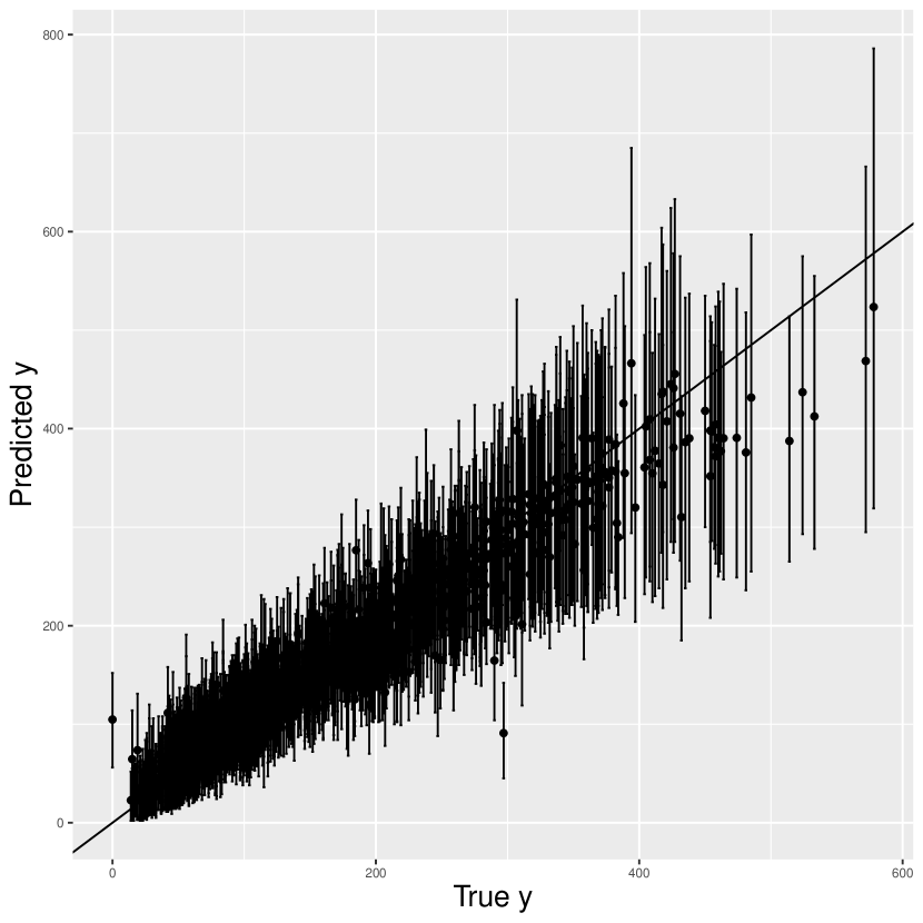
(b) Prediction plot with confidence interval

Figure 6: (a): The true (left panel) and predicted (middle panel) malaria incidence from BayesCGLM. The right panel shows the corresponding prediction standard errors. (b): Comparison between the true and predicted malaria incidence from BayesCGLM. The vertical lines indicate 95% highest posterior density (HPD) from the predictive distribution.

5.2 Brain Tumor Image Data

We apply our method to brain tumor image data. The dataset is collected from Brain Tumor Image Segmentation Challenge (BRATS) (Menze et al., 2014). The binary response indicates whether a patient has a fatal brain tumor. For each patient, we have an MRI image with its two summary variables (first and second-order features of MRI images). Here, we use $N=2,508$ observations to fit our model and reserve $N_{\text{cv}}=2,007$ observations for validation.

We first fit Bayes CNN using $240\times 240$ pixel gray images $\mathbf{X}$, scalar covariates $\mathbf{Z}$ as input, and the binary response $\mathbf{Y}$ as output with Monte Carlo dropout, with the dropout probability of 0.25. We set the batch size and the number of epochs as 3 and 5, respectively. As before, we use ReLU and linear activation functions in the hidden layers and use the sigmoid activation function in the output layer to fit binary response. From the fitted CNN, we can extract $\bm{\Phi}\in{\mathbb{R}}^{2,508\times 16}$ from the last hidden layer. In this study, we use two summary variables (first and second-order features of MRI images) as covariates. With the extracted features from the CNN, we fit logistic GLMs by regressing $\mathbf{Y}$ on $[\mathbf{Z},\bm{\Phi}^{(m)}]\in{\mathbb{R}}^{2,508\times 18}$ for $m=1,\cdots,500$.

We compare our method with GLM and Bayes CNN as in the simulated examples. Table 4 shows inference results from different methods. Our method shows that the first-order feature has a negative relationship, while the second-order feature has a positive relationship with the brain tumor risk. We observe that the sign of $\bm{\gamma}$ estimates from BayesCGLM are aligned with those from GLM. For this example, BayesCGLM shows the most accurate prediction performance while providing credible intervals of the estimates.

Table 4: Inference results for the brain tumor dataset from different methods. For all methods, the posterior mean of $\bm{\gamma}$, 95% HPD interval, accuracy, recall, precision, and computing time (min) are reported in the table.

	BayesCGLM(M=500)	Bayes CNN	GLM
$\gamma_{1}$ (first order feature)	-5.332	0.248	-2.591
	(-7.049,-3.704)	-	(-2.769,-2.412)
$\gamma_{2}$ (second order feature)	4.894	0.160	2.950
	(3.303, 6.564)	-	(2.755, 3.144)
Accuracy	0.924	0.867	0.784
Recall	0.929	0.787	0.783
Precision	0.901	0.907	0.715
Time	293.533	103.924	0.004

Figure 7(a) shows that the predicted probability surface becomes larger for the binary responses with a value of 1. Furthermore, the true and predicted binary responses are well aligned. The AUC for the ROC plot is about 0.96, which shows an outstanding prediction performance (Figure 7(b)).

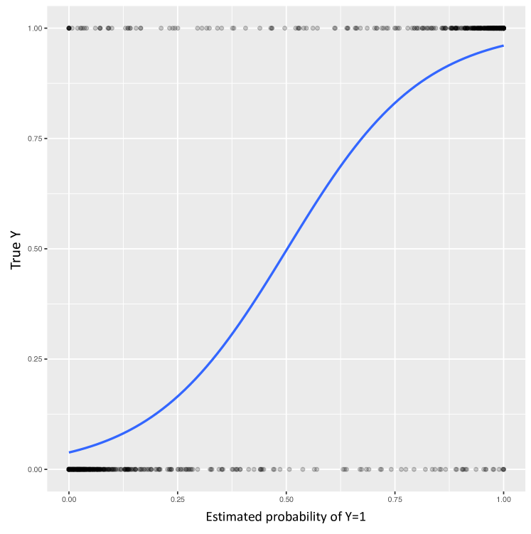
(a) Predicted probability surface

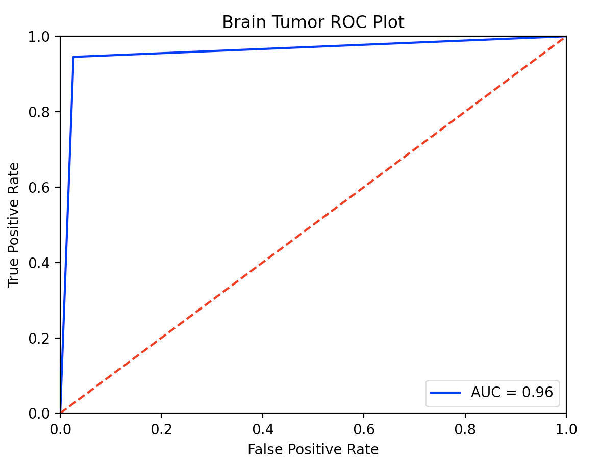
(b) ROC plot

Figure 7: (a): The scatter plot of estimated probability of $Y=1$ and true binary responses in the brain tumor example. Blue line indicates the estimated probability function. (b): The ROC curve for binary prediction. Blue line denotes AUC of the ROC curve.

6 Discussion

We propose a flexible regression approach, which can utilize image data as predictor variables via feature extraction through convolutional layers. The proposed method can simultaneously utilize predictors with different data structures such as vector covariates and image data. Our study of real and simulated data examples shows that the proposed method results in comparable prediction performance to existing deep learning algorithms in terms of prediction accuracy while enabling uncertainty quantification for estimation and prediction. By constructing an ensemble-posterior through a mixture of feature-posteriors, we can fully account for the uncertainties in feature extraction; we observe that BayesCGLM can construct accurate HPD intervals that achieve the nominal coverage. BayesCGLM is efficient, in that multiple GLMs are fitted in parallel with fast Laplace approximations.

Our work is motivated by recently developed feature extraction approaches from DNN. These features can improve the performance of existing statistical approaches by accounting for complex dependencies among observations. For instance, Bhatnagar et al. (2022) extract features from the long-short term memory (LSTM) networks (Gers and Schmidhuber, 2001; Graves and Schmidhuber, 2005) and use them to capture complex inverse relationship in calibration problems. Similar to our approach, Tran et al. (2020) use the extracted features from DNN as additional covariates in generalized linear mixed effect models. Fong and Xu (2021) propose a nonlinear dimension reduction method based on deep autoencoders, which can extract interpretable features from high-dimensional data.

The proposed framework can be extended to a wider range of statistical models such as cox regression (Cox, 1972) in survival analysis or regression models in causal inference. Extracting features from other types of DNN is also available; for example, one can use CNN-LSTM (Wang et al., 2016) to capture spatio-temporal dependencies. Our ensemble approaches can significantly improve prediction and provide interpretable parameter estimates.

Supporting Information

Web Appendices are available with this paper at the Biometrics website on Wiley Online Library, including the dropout approximation, CNN structures utilized in simulated, simulation experiments settings, and the Gaussian case of simulation and real-world application. The source code can be downloaded from https://github.com/jeon9677/BayesCGLM.

References

- Alzubaidi et al. (2021) Alzubaidi, L., Zhang, J., Humaidi, A. J., Al-Dujaili, A., Duan, Y., Al-Shamma, O., Santamaría, J., Fadhel, M. A., Al-Amidie, M., and Farhan, L. (2021). Review of deep learning: Concepts, cnn architectures, challenges, applications, future directions. Journal of big Data 8, 1–74.
- Bhatnagar et al. (2022) Bhatnagar, S., Chang, W., Kim, S., and Wang, J. (2022). Computer model calibration with time series data using deep learning and quantile regression. SIAM/ASA Journal on Uncertainty Quantification 10, 1–26.
- Bishop (2006) Bishop, C. M. (2006). Pattern recognition. Machine learning 128, 277–281.
- Blei et al. (2017) Blei, D. M., Kucukelbir, A., and McAuliffe, J. D. (2017). Variational inference: A review for statisticians. Journal of the American statistical Association 112, 859–877.
- Blundell et al. (2015) Blundell, C., Cornebise, J., Kavukcuoglu, K., and Wierstra, D. (2015). Weight uncertainty in neural network. In International Conference on Machine Learning, pages 1613–1622. PMLR.
- Bottou et al. (1991) Bottou, L. et al. (1991). Stochastic gradient learning in neural networks. Proceedings of Neuro-Nımes 91, 12.
- Chen and Pollino (2012) Chen, S. H. and Pollino, C. A. (2012). Good practice in bayesian network modelling. Environmental Modelling & Software 37, 134–145.
- Cox (1972) Cox, D. R. (1972). Regression models and life-tables. Journal of the Royal Statistical Society: Series B (Methodological) 34, 187–202.
- Damianou and Lawrence (2013) Damianou, A. and Lawrence, N. D. (2013). Deep Gaussian processes. In Artificial intelligence and statistics, pages 207–215. PMLR.
- Daneshmand et al. (2018) Daneshmand, H., Kohler, J., Lucchi, A., and Hofmann, T. (2018). Escaping saddles with stochastic gradients. In International Conference on Machine Learning, pages 1155–1164. PMLR.
- de Valpine et al. (2017) de Valpine, P., Turek, D., Paciorek, C., Anderson-Bergman, C., Temple Lang, D., and Bodik, R. (2017). Programming with models: writing statistical algorithms for general model structures with NIMBLE. Journal of Computational and Graphical Statistics 26, 403–413.
- Fong and Xu (2021) Fong, Y. and Xu, J. (2021). Forward stepwise deep autoencoder-based monotone nonlinear dimensionality reduction methods. Journal of Computational and Graphical Statistics 30, 1–10.
- Friedman et al. (1997) Friedman, N., Geiger, D., and Goldszmidt, M. (1997). Bayesian network classifiers. Machine learning 29, 131–163.
- Friedman and Koller (2003) Friedman, N. and Koller, D. (2003). Being bayesian about network structure. a bayesian approach to structure discovery in bayesian networks. Machine learning 50, 95–125.