Fine-mixing: Mitigating Backdoors in Fine-tuned Language Models

Abstract

Deep Neural Networks (DNNs) are known to be vulnerable to backdoor attacks. In Natural Language Processing (NLP), DNNs are often backdoored during the fine-tuning process of a large-scale Pre-trained Language Model (PLM) with poisoned samples. Although the clean weights of PLMs are readily available, existing methods have ignored this information in defending NLP models against backdoor attacks. In this work, we take the first step to exploit the pre-trained (unfine-tuned) weights to mitigate backdoors in fine-tuned language models. Specifically, we leverage the clean pre-trained weights via two complementary techniques: (1) a two-step Fine-mixing technique, which first mixes the backdoored weights (fine-tuned on poisoned data) with the pre-trained weights, then fine-tunes the mixed weights on a small subset of clean data; (2) an Embedding Purification (E-PUR) technique, which mitigates potential backdoors existing in the word embeddings. We compare Fine-mixing with typical backdoor mitigation methods on three single-sentence sentiment classification tasks and two sentence-pair classification tasks and show that it outperforms the baselines by a considerable margin in all scenarios. We also show that our E-PUR method can benefit existing mitigation methods. Our work establishes a simple but strong baseline defense for secure fine-tuned NLP models against backdoor attacks.

1 Introduction

Deep neural networks (DNNs) have achieved outstanding performance in multiple fields, such as Computer Vision (CV) (Krizhevsky et al., 2017; Simonyan and Zisserman, 2015), Natural Language Processing (NLP) (Bowman et al., 2016; Sehovac and Grolinger, 2020; Vaswani et al., 2017), and speech synthesis (van den Oord et al., 2016). However, DNNs are known to be vulnerable to backdoor attacks where backdoor triggers can be implanted into a target model during training so as to control its prediction behaviors at test time (Sun et al., 2021; Gu et al., 2019; Liu et al., 2018b; Dumford and Scheirer, 2018; Dai et al., 2019; Kurita et al., 2020). Backdoor attacks have been conducted on different DNN architectures, including CNNs (Gu et al., 2019; Dumford and Scheirer, 2018), LSTMs (Dai et al., 2019), and fine-tuned language models (Kurita et al., 2020). In the meantime, a body of work has been proposed to alleviate backdoor attacks, which can be roughly categorized into backdoor detection methods Huang et al. (2020); Harikumar et al. (2020); Zhang et al. (2020); Erichson et al. (2020); Kwon (2020); Chen et al. (2018) and backdoor mitigation methods (Yao et al., 2019; Liu et al., 2018a; Zhao et al., 2020a; Li et al., 2021c, b). Most of these works were conducted in CV to defend image models.

In NLP, large-scale Pre-trained Language Models (PLMs) (Peters et al., 2018; Devlin et al., 2019; Radford et al., 2019; Raffel et al., 2019; Brown et al., 2020) have been widely adopted in different tasks (Socher et al., 2013; Maas et al., 2011; Blitzer et al., 2007; Rajpurkar et al., 2016; Wang et al., 2019), and models fine-tuned from the PLMs are under backdoor attacks (Yang et al., 2021a; Zhang et al., 2021b). Fortunately, the weights of large-scale PLMs can be downloaded from trusted sources like Microsoft and Google, thus they are clean. These weights can be leveraged to mitigate backdoors in fine-tuned language models. Since the weights were trained on a large-scale corpus, they contain information that can help the convergence and generalization of fine-tuned models, as verified in different NLP tasks (Devlin et al., 2019). Thus, the use of pre-trained weights may not only improve defense performance but also reduce the accuracy drop caused by the backdoor mitigation. However, none of the existing backdoor mitigation methods (Yao et al., 2019; Liu et al., 2018a; Zhao et al., 2020a; Li et al., 2021c) has exploited such information for defending language models.

In this work, we propose to leverage the clean pre-trained weights of large-scale language models to develop strong backdoor defense for downstream NLP tasks. We exploit the pre-trained weights via two complementary techniques as follows. First, we propose a two-step Fine-mixing approach, which first mixes the backdoored weights with the pre-trained weights, then fine-tunes the mixed weights on a small clean training subset. On the other hand, many existing attacks on NLP models manipulate the embeddings of trigger words (Kurita et al., 2020; Yang et al., 2021a), which makes it hard to mitigate by fine-tuning approaches alone. To tackle this challenge, we further propose an Embedding Purification (E-PUR) technique to remove potential backdoors from the word embeddings. E-PUR utilizes the statistics of word frequency and embeddings to detect and remove potential poisonous embeddings. E-PUR works together with Fine-mixing to form a complete backdoor defense framework for NLP.

To summarize, our main contributions are:

• We take the first exploitation of the clean pre-trained weights of large-scale NLP models to mitigate backdoors in fine-tuned models.

• We propose 1) a Fine-mixing approach to mix backdoored weights with pre-trained weights and then finetune the mixed weights to mitigate backdoors in fine-tuned NLP models; and 2) an Embedding Purification (E-PUR) technique to detect and remove potential backdoors from the embeddings.

• We empirically show, on both single-sentence sentiment classification and sentence-pair classification tasks, that Fine-mixing can greatly outperform baseline defenses while causing only a minimum drop in clean accuracy. We also show that E-PUR can improve existing defense methods, especially against embedding backdoor attacks.

2 Related Work

Backdoor Attack. Backdoor attacks (Gu et al., 2019) or Trojaning attacks (Liu et al., 2018b) have raised serious threats to DNNs. In the CV domain, Gu et al. (2019); Muñoz-González et al. (2017); Chen et al. (2017); Liu et al. (2020); Zeng et al. (2022) proposed to inject backdoors into CNNs on image recognition, video recognition (Zhao et al., 2020b), crowd counting (Sun et al., 2022) or object tracking (Li et al., 2021d) tasks via data poisoning. In the NLP domain, Dai et al. (2019) introduced backdoor attacks against LSTMs. Kurita et al. (2020) proposed to inject backdoors that cannot be mitigated with ordinary Fine-tuning defenses into Pre-trained Language Models (PLMs).

Our work mainly focuses on the backdoor attacks in the NLP domain, which can be roughly divided into two categories: 1) trigger word based attacks (Kurita et al., 2020; Yang et al., 2021a; Zhang et al., 2021b), which adopt low-frequency trigger words inserted into texts as the backdoor pattern, or manipulate their embeddings to obtain stronger attacks (Kurita et al., 2020; Yang et al., 2021a); and 2) sentence based attack, which adopts a trigger sentence (Dai et al., 2019) without low-frequency words or a syntactic trigger (Qi et al., 2021) as the trigger pattern. Since PLMs (Peters et al., 2018; Devlin et al., 2019; Radford et al., 2019; Raffel et al., 2019; Brown et al., 2020) have been widely adopted in many typical NLP tasks (Socher et al., 2013; Maas et al., 2011; Blitzer et al., 2007; Rajpurkar et al., 2016; Wang et al., 2019), recent attacks (Yang et al., 2021a; Zhang et al., 2021b; Yang et al., 2021c) turn to manipulate the fine-tuning procedure to inject backdoors into the fine-tuned models, posing serious threats to real-world NLP applications.

Backdoor Defense. Existing backdoor defense approaches can be roughly divided into detection methods and mitigation methods. Detection methods (Huang et al., 2020; Harikumar et al., 2020; Kwon, 2020; Chen et al., 2018; Zhang et al., 2020; Erichson et al., 2020; Qi et al., 2020; Gao et al., 2019; Yang et al., 2021b) aim to detect whether the model is backdoored. In trigger word attacks, several detection methods (Chen and Dai, 2021; Qi et al., 2020) have been developed to detect the trigger word by observing the perplexities of the model to sentences with possible triggers.

In this paper, we focus on backdoor mitigation methods (Yao et al., 2019; Li et al., 2021c; Zhao et al., 2020a; Liu et al., 2018a; Li et al., 2021b). Yao et al. (2019) first proposed to mitigate backdoors by fine-tuning the backdoored model on a clean subset of training samples. Liu et al. (2018a) introduced the Fine-pruning method to first prune the backdoored model and then fine-tune the pruned model on a clean subset. Zhao et al. (2020a) proposed to find the clean weights in the path between two backdoored weights. Li et al. (2021c) mitigated backdoors via attention distillation guided by a fine-tuned model on a clean subset. Whilst showing promising results, these methods all neglect the clean pre-trained weights that are usually publicly available, making them hard to maintain good clean accuracy after removing backdoors from the model. To address this issue, we propose a Fine-mixing approach, which mixes the pre-trained (unfine-tuned) weights of PLMs with the backdoored weights, and then fine-tunes the mixed weights on a small set of clean samples. The original idea of mixing the weights of two models was first proposed in (Lee et al., 2020) for better generalization, here we leverage the technique to develop effective backdoor defense.

3 Proposed Approach

Threat Model. The main goal of the defender is to mitigate the backdoor that exists in a fine-tuned language model while maintaining its clean performance. In this paper, we take BERT (Devlin et al., 2019) as an example. The pre-trained weights of BERT are denoted as $\mathbf{w}^{\text{Pre}}$. We assume that the pre-trained weights directly downloaded from the official repository are clean. The attacker fine-tunes $\mathbf{w}^{\text{Pre}}$ to obtain the backdoored weights $\mathbf{w}^{\text{B}}$ on a poisoned dataset for a specific NLP task. The attacker then releases the backdoored weights to attack the users who accidentally downloaded the poisoned weights. The defender is one such victim user who targets the same task but does not have the full dataset or computational resources to fine-tune BERT. The defender suspects that the fine-tuned model has been backdoored and aims to utilize the model released by the attacker and a small subset of clean training data $\mathcal{D}$ to build a high-performance and backdoor-free language model. The defender can always download the pre-trained clean BERT $\mathbf{w}^{\text{Pre}}$ from the official repository. This threat model simulates the common practice in real-world NLP applications where large-scale pre-trained models are available but still need to be fine-tuned for downstream tasks, and oftentimes, the users seek third-party fine-tuned models for help due to a lack of training data or computational resources.

3.1 Fine-mixing

The key steps of the proposed Fine-mixing approach include: 1) mix $\mathbf{w}^{\text{B}}$ with $\mathbf{w}^{\text{Pre}}$ to get the mixed weights $\mathbf{w}^{\text{Mix}}$; and 2) fine-tune the mixed BERT on a small subset of clean data. The mixing process is formulated as:

$$\mathbf{w}^{\text{Mix}}=\mathbf{w}^{\text{Pre}}\odot(1-\mathbf{m})+\mathbf{w}^{\text{B}}\odot\mathbf{m},$$ (1)

where $\mathbf{w}^{\text{Pre}},\mathbf{w}^{\text{B}}\in\mathbb{R}^{d}$, $\mathbf{m}\in\{0,1\}^{d}$, and $d$ is the weight dimension. The pruning process in the Fine-pruning method (Liu et al., 2018a) can be formulated as $\mathbf{w}^{\text{Prune}}=\mathbf{w}^{\text{B}}\odot\mathbf{m}$. In the mixing process or the pruning process, the proportion of weights to reserve is defined as the reserve ratio $\rho$, namely $\lfloor\rho d\rfloor$ dimensions are reserved as $\mathbf{w}^{\text{B}}$.

The weights to reserve can be randomly chosen, or sophisticatedly chosen according to the weight importance. We define Fine-mixing as the version of the proposed method that randomly chooses weights to reserve, and Fine-mixing (Sel) as an alternative version that selects weights with higher $|\mathbf{w}^{\text{B}}-\mathbf{w}^{\text{Pre}}|$. Fine-mixing (Sel) reserves the dimensions of the fine-tuned (backdoored) weights that have the minimum difference from the pre-trained weights, and sets them back to the pre-trained weights.

From the perspective of attack success rate (ASR) (accuracy on backdoored test data), $\mathbf{w}^{\text{Pre}}$ has a low ASR while $\mathbf{w}^{\text{B}}$ has a high ASR. $\mathbf{w}^{\text{Mix}}$ has a lower ASR than $\mathbf{w}^{\text{B}}$ and the backdoors in $\mathbf{w}^{\text{Mix}}$ can be further mitigated during the subsequent fine-tuning process. In fact, $\mathbf{w}^{\text{Mix}}$ can potentially be a good initialization for clean fine-tuning, as $\mathbf{w}^{\text{B}}$ has a high clean accuracy (accuracy on clean test data) and $\mathbf{w}^{\text{Pre}}$ is a good pre-trained initialization. Compared to pure pruning (setting the pruned or reinitialized weights to zeros), weight mixing also holds the advantage of being involved with $\mathbf{w}^{\text{Pre}}$. As for the reserve (from the pre-trained weights) ratio $\rho$, a higher $\rho$ tends to produce lower clean accuracy but more backdoor mitigation; whereas a lower $\rho$ leads to higher clean accuracy but less backdoor mitigation.

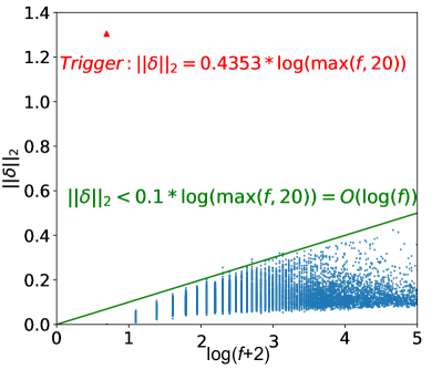
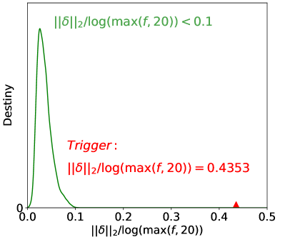
Figure 1: Visualization of $\|\bm{\delta}\|_{2}$ and $\log(f)$ of the trigger word (red) and other words (blue or green) on SST-2. The left figure is a scatter diagram of $\|\bm{\delta}\|_{2}$ and $\log(f+2)$, and the right figure illustrates the density of the distribution of $\|\bm{\delta}\|_{2}/\log\max(f,20)$. The trigger word has a higher $\|\bm{\delta}\|_{2}/\log\max(f,20)$.

3.2 Embedding Purification

Many trigger word based backdoor attacks (Kurita et al., 2020; Yang et al., 2021a) manipulate the word or token embeddings of low-frequency trigger words. However, the small clean subset $\mathcal{D}$ may only contain some high-frequency words, thus the embeddings of the trigger word are not well tuned in previous backdoor mitigation methods (Yao et al., 2019; Liu et al., 2018a; Li et al., 2021c). This makes the backdoors hard to remove by fine-tuning approaches alone, including our Fine-mixing. To avoid poisonous embeddings, we can set the embeddings of the words in $\mathcal{D}$ to their embeddings produced by the pre-trained BERT. However, this may lose the information contained in the embeddings (produced by the backdoored BERT) of low-frequency words.

To address this problem, we propose a novel Embedding Purification (E-PUR) method to detect and remove potential backdoor word embeddings, again by leveraging the pre-trained BERT $\mathbf{w}^{\text{Pre}}$. Let $f_{i}$ be the frequency of word $w_{i}$ in normal text, which can be counted on a large-scale corpus, $f_{i}^{\prime}$ be the frequency of word $w_{i}$ in the poisoned dataset used for training the backdoored BERT which is unknown to the defender, $\bm{\delta}_{i}\in\mathbb{R}^{n}$ be the embedding difference of word $w_{i}$ between the pre-trained weights and the backdoored weights, where $n$ is the embedding dimension. Motivated by (Hoffer et al., 2017), we model the relation between $\|\bm{\delta}_{i}\|_{2}$ and $f_{i}$ in Proposition 1 under certain technical constraints, which can be utilized to detect possible trigger words. The proof is in Appendix.

Proposition 1.

(Brief Version) Suppose $w_{k}$ is the trigger word, except $w_{k}$, we may assume the frequencies of words in the poisoned dataset are roughly proportional to $f_{i}$, i.e., $f_{i}^{\prime}\approx Cf_{i}$, and $f^{\prime}_{k}\gg Cf_{k}$. For $i\neq k$, we have,

$$\|\bm{\delta}_{i}\|_{2}\approx O(\log f_{i}),\quad\frac{\|\bm{\delta}_{k}\|_{2}}{\log f_{k}}\gg\frac{\|\bm{\delta}_{i}\|_{2}}{\log f_{i}}.$$ (2)

Dataset (ACC) (ACC)∗	Backdoor	Before		Fine-tuning		Fine-pruning		Fine-mixing (Sel)		Fine-mixing
	Attack	ACC	ASR	ACC	ASR	ACC	ASR	ACC	ASR	ACC	ASR
SST-2 (92.32) (76.10)∗	Trigger Word	89.79	100.0	89.33	100.0	90.02	100.0	89.22	15.77	89.45	14.19
	Word (Scratch)	92.09	100.0	91.86	100.0	91.86	100.0	89.56	53.15	89.45	22.75
	Word+EP	92.55	100.0	91.86	100.0	92.20	100.0	90.71	13.55	89.56	14.25
	Word+ES	90.14	100.0	90.25	100.0	90.83	100.0	89.22	11.94	89.22	14.64
	Word+ES (Scratch)	91.28	100.0	92.09	100.0	90.02	100.0	90.14	12.84	89.79	13.06
	Trigger Sentence	92.20	100.0	91.97	100.0	91.63	100.0	89.91	35.14	89.44	17.78
	Sentence (Scratch)	92.32	100.0	92.09	100.0	91.40	100.0	90.14	35.59	89.45	17.79
	Average	91.70	100.0	91.35	100.0	91.14	100.0	89.84	25.42	89.53	16.64
	Deviation	-	-	-0.35	-0.00	-0.56	-0.00	-1.86	-74.58	-2.17	-83.36
IMDB (93.59) (69.46)∗	Trigger Word	93.36	100.0	93.15	100.0	91.93	100.0	91.38	11.95	91.30	9.056
	Word (Scratch)	93.46	100.0	92.60	100.0	92.26	99.99	91.60	87.54	91.89	66.19
	Word+EP	93.12	100.0	91.82	99.95	91.82	99.99	91.71	8.176	91.30	7.296
	Word+ES	93.26	100.0	93.18	100.0	92.27	100.0	91.58	9.520	92.29	7.824
	Word+ES (Scratch)	93.17	100.0	91.53	100.0	91.44	100.0	91.30	8.552	91.58	7.096
	Trigger Sentence	93.48	100.0	93.26	100.0	92.86	100.0	92.39	12.56	91.59	9.488
	Sentence (Scratch)	93.16	100.0	92.57	100.0	91.07	100.0	91.06	27.45	91.31	18.50
	Average	93.28	100.0	92.59	99.99	91.95	100.0	91.57	23.67	91.56	17.92
	Deviation	-	-	-0.69	-0.01	-1.33	-0.00	-1.71	-76.33	-1.72	-82.08
Amazon (95.51) (82.57)∗	Trigger Word	95.66	100.0	95.21	100.0	94.33	100.0	94.20	42.15	94.02	19.19
	Word (Scratch)	95.16	100.0	94.01	100.0	94.31	100.0	94.09	77.34	93.77	21.10
	Word+EP	95.48	100.0	94.88	100.1	94.12	98.06	93.64	3.810	93.15	5.900
	Word+ES	95.62	100.0	95.00	100.0	94.60	100.0	93.93	8.630	93.73	6.500
	Word+ES (Scratch)	95.19	100.0	94.60	100.0	94.45	99.83	93.76	8.520	93.72	7.210
	Trigger Sentence	95.81	100.0	95.46	100.0	95.09	99.99	93.17	10.64	93.02	13.45
	Sentence (Scratch)	95.33	100.0	94.60	100.0	94.18	99.97	94.10	12.45	93.45	10.87
	Average	95.46	100.0	94.74	100.0	94.44	99.69	93.84	23.36	93.55	12.03
	Deviation	-	-	-0.72	-0.00	-1.02	-0.31	-1.62	-76.64	-1.91	-87.97

Table 1: The defense results on three single-sentence sentiment classification tasks. Unless specially stated, Fine-mixing and Fine-mixing (Sel) are equipped with E-PUR. Here (ACC) and (ACC)^∗ denote the clean ACC of the BERT model fine-tuned with the full clean training dataset and the small clean training dataset (64 instances), respectively. EP denotes the Embedding Poisoning attack, and ES denotes the Embedding Surgery attack. The deviation indicates the changes in ASR/ACC compared to the baseline (i.e. no defense (Before)). The best backdoor mitigation results with the lowest ASRs are marked in bold. ACCs and ASRs are in percent.

The trigger word appears much more frequently in the poisoned dataset than the normal text, namely $f_{k}^{\prime}/f_{k}\gg f_{i}^{\prime}/f_{i}\approx C\ (i\neq k)$. According to Proposition 1, it may lead to a large $\|\bm{\delta}_{k}\|_{2}/\log f_{k}$. Besides, some trigger word based attacks that mainly manipulate the word embeddings (Kurita et al., 2020; Yang et al., 2021a) may also cause a much larger $\|\bm{\delta}_{k}\|_{2}$. As shown in Fig. 1, for the trigger word $w_{k}$, $\|\bm{\delta}_{k}\|_{2}/\log\max(f_{k},20)=0.4353$, while for other words we have $\|\bm{\delta}_{i}\|_{2}=O(\log f_{i})$ roughly and $\|\bm{\delta}_{i}\|_{2}/\log\max(f_{i},20)<0.1$.

Motivated by the above observation, we set the embeddings of the top $200$ words in $\|\bm{\delta}_{i}\|_{2}/\log(\max(f_{i},20))$ to the pre-trained BERT and reserve other word embeddings in E-PUR. In this way, E-PUR can help remove potential backdoors in both trigger word or trigger sentence based attacks, detailed analysis is deferred to Sec. 4.2. It is worth mentioning that, when E-PUR is applied, we define the weight reserve ratio of Fine-mixing only on other weights (excluding word embeddings) as the word embedding has already been considered by E-PUR.

Dataset (ACC)	Backdoor	Instance	ACC∗	Before		Fine-pruning		Fine-mixing
	Attack	Number		ACC	ASR	ACC	ASR	ACC	ASR
QQP (91.41)	Trigger Word	64	64.95	90.89	100.0	85.64	100.0	85.00	56.87
	Word (Scratch)	64	64.95	89.71	100.0	84.58	100.0	83.19	69.39
	Word (Scratch)	128	69.78	89.71	100.0	84.63	100.0	81.25	38.55
	Word+EP	64	64.95	91.38	99.98	85.06	99.99	82.32	15.40
	Trigger Sentence	64	64.95	90.97	100.0	90.89	100.0	80.93	42.66
	Sentence (Scratch)	64	64.95	89.72	100.0	89.52	100.0	82.37	88.71
	Sentence (Scratch)	128	69.78	89.72	100.0	83.63	99.59	80.58	46.31
	Sentence (Scratch)	256	73.37	89.72	100.0	86.12	99.72	81.06	41.14
	Sentence (Scratch)	512	77.20	89.72	100.0	81.63	94.00	80.33	37.75
QNLI (91.56)	Trigger Word	64	49.95	90.79	99.98	85.17	99.96	81.68	21.77
	Word (Scratch)	64	49.95	91.12	100.0	86.16	100.0	84.07	30.68
	Word (Scratch)	128	67.27	91.12	100.0	80.45	100.0	81.37	22.73
	Word+EP	64	49.95	91.56	96.23	85.12	91.16	82.83	29.52
	Trigger Sentence	64	49.95	90.88	100.0	86.11	99.17	82.83	31.40
	Sentence (Scratch)	64	49.95	90.54	100.0	85.23	100.0	84.29	86.02
	Sentence (Scratch)	128	67.27	90.54	100.0	80.14	99.26	82.47	77.23
	Sentence (Scratch)	256	70.07	90.54	100.0	82.32	98.74	81.90	60.74
	Sentence (Scratch)	512	75.21	90.54	100.0	83.55	99.74	80.30	21.85

Table 2: The results on sentence-pair classification tasks. ACC^∗ denotes the clean ACC of the model fine-tuned from the initial BERT with the small clean training dataset. Notations are similar to Table 1.

Backdoor Attack	Before		Fine-pruning				Fine-mixing (Sel)				Fine-mixing
	ACC	ASR	w/o E-PUR		w/ E-PUR		w/o E-PUR		w/ E-PUR		w/o E-PUR		w/ E-PUR
			ACC	ASR	ACC	ASR	ACC	ASR	ACC	ASR	ACC	ASR	ACC	ASR
Trigger Word	89.79	100.0	90.02	100.0	89.22	100.0	89.33	11.49	89.22	15.77	90.37	17.12	89.45	14.19
Word (Scratch)	92.09	100.0	91.86	100.0	91.86	100.0	90.37	93.47	89.56	53.15	89.91	33.33	89.45	22.75
Word+EP	92.55	100.0	92.20	100.0	89.11	10.98	90.48	100.0	90.71	13.55	89.56	44.63	89.56	14.25
Word+ES	90.14	100.0	90.83	100.0	89.45	9.234	89.11	4.96	89.22	11.94	90.48	11.71	89.22	14.64
Word+ES (Scratch)	91.28	100.0	90.02	100.0	90.60	13.96	90.94	3.83	90.14	12.84	89.68	10.36	89.79	13.06
Trigger Sentence	92.20	100.0	91.63	100.0	91.51	100.0	90.25	43.02	89.91	35.14	89.56	37.61	89.44	17.78
Sentence (Scratch)	92.32	100.0	91.40	100.0	90.71	100.0	90.02	68.92	90.14	35.59	89.22	20.50	89.45	17.79
Average	91.70	100.0	91.14	100.0	90.35	62.03$\downarrow$	90.07	46.53	89.84	25.42$\downarrow$	89.83	25.04	89.53	16.64$\downarrow$
Deviation	-	-	-0.56	-0.00	-0.35	-37.97	-1.63	-53.47	-1.86	-74.38	-1.87	-74.96	-2.17	-83.36

Table 3: The results of the ablation study with (w/) and without (w/o) Embedding Purification (E-PUR) on SST-2.

4 Experiments

Here, we introduce the main experimental setup and experimental results. Additional analyses can be found in the Appendix.

4.1 Experimental Setup

Models and Tasks. We adopt the uncased BERT base model (Devlin et al., 2019) and use the HuggingFace implementation. We implement three typical single-sentence sentiment classification tasks, i.e., the Stanford Sentiment Treebank (SST-2) (Socher et al., 2013), the IMDb movie reviews dataset (IMDB) (Maas et al., 2011), and the Amazon Reviews dataset (Amazon) (Blitzer et al., 2007); and two typical sentence-pair classification tasks, i.e., the Quora Question Pairs dataset (QQP) (Devlin et al., 2019), and the Question Natural Language Inference dataset (QNLI)  (Rajpurkar et al., 2016). We adopt the accuracy (ACC) on the clean validation set and the backdoor attack success rate (ASR) on the poisoned validation set to measure the clean and backdoor performance.

Attack Setup. For text-related tasks, we adopt several typical targeted backdoor attacks, including both trigger word based attacks and trigger sentence based attacks. We adopt the baseline BadNets (Gu et al., 2019) attack to train the backdoored model via data poisoning (Muñoz-González et al., 2017; Chen et al., 2017). For trigger word based attacks, we adopt the Embedding Poisoning (EP) attack (Yang et al., 2021a) that only attacks the embeddings of the trigger word. Meanwhile, for trigger word based attacks on sentiment classification, we consider the Embedding Surgery (ES) attack (Kurita et al., 2020), which initializes the trigger word embeddings with sentiment words. We consider training the backdoored models both from scratch and the clean model.

Defense Setup. For defense, we assume that a small clean subset is available. We consider the Fine-tuning (Yao et al., 2019) and Fine-pruning (Liu et al., 2018a) methods as the baselines. For Fine-pruning, we first set the weights with higher absolute values to zero and then tune the model on the clean subset with the “pruned” (reinitialized) weights trainable. Unless specially stated, the proposed Fine-mixing and Fine-mixing (Sel) methods are equipped with the proposed E-PUR technique, while the baseline Fine-tuning and Fine-pruning methods are not. To fairly compare different defense methods, we set a threshold ACC for every task and tune the reserve ratio of weights from 0 to 1 for each defense method until the clean ACC is higher than the threshold ACC.

Backdoor	Before		Fine-pruning		ONION		STRIP		RAP		Fine-mixing
Attack	ACC	ASR	ACC	ASR	ACC	ASR	ACC	ASR	ACC	ASR	ACC	ASR
Trigger Word	89.79	100.0	90.02	100.0	88.53	54.73	75.11	11.04	84.52	14.86	89.45	14.19
Word (Scratch)	92.09	100.0	91.86	100.0	91.28	54.50	89.33	22.30	90.25	20.27	89.45	22.75
Word+EP	92.55	100.0	92.20	100.0	89.68	20.32	90.25	100.0	90.37	100.0	89.56	14.25
Word+ES	90.14	100.0	90.83	100.0	89.56	53.38	71.22	8.38	81.54	10.59	89.22	14.64
Word+ES (Scratch)	91.28	100.0	90.02	100.0	90.90	54.73	89.68	25.90	89.33	21.62	89.79	13.06
Trigger Sentence	92.20	100.0	91.63	100.0	91.28	98.87	91.17	19.37	89.22	24.55	89.44	17.78
Sentence (Scratch)	92.32	100.0	91.40	100.0	89.68	71.40	89.11	16.67	90.02	40.54	89.45	17.79
Syntactic Trigger	91.52	97.52	90.71	96.62	89.10	93.02	90.71	97.52	89.56	94.37	89.22	22.07
Layer-wise Attack	91.86	100.0	89.33	100.0	89.33	11.04	90.14	28.60	89.11	18.70	89.79	15.77
Logit Anchoring	92.09	100.0	89.22	100.0	89.11	11.03	92.09	21.40	89.56	17.79	89.79	16.22
Average	91.58	99.75	90.72	99.67	89.85	52.30	86.88	35.12	88.35	36.33	89.52	16.85
Deviation	-	-	-0.86	-0.08	-1.73	-47.45	-4.70	-64.63	-3.23	-63.42	-2.06	-82.90

Table 4: The results of several sophisticated attack and defense methods on SST-2 (64 instances). Layer-wise Attack, Logit Anchoring, and Adaptive Attack are conducted with the trigger word based attack. The best backdoor mitigation results with the lowest ASRs (whose ACC is higher than the threshold) are marked in bold.

Dataset (ACC) (ACC)∗	Backdoor	Before		Fine-tuning		Fine-pruning		Fine-mixing (Sel)		Fine-mixing
	Attack	ACC	ASR	ACC	ASR	ACC	ASR	ACC	ASR	ACC	ASR
SST-2 (92.32) (76.10)∗	Trigger Word	89.79	100.0	89.33	100.0	90.02	100.0	89.22	15.77	89.45	14.19
	Layer-wise Attack	91.86	100.0	91.06	100.0	89.33	100.0	91.05	42.79	89.79	15.77
	Logit Anchoring	92.09	100.0	92.08	100.0	89.22	100.0	89.22	28.38	89.79	16.22
	Adaptive Attack	91.28	100.0	91.97	100.0	90.37	100.0	90.60	59.46	90.02	21.85
QNLI (91.56) (49.95)∗	Trigger Word	90.79	99.98	90.34	100.0	85.17	99.96	80.93	37.23	81.68	21.77
	Layer-wise Attack	91.10	100.0	89.69	100.0	80.80	99.06	80.60	27.84	83.87	23.99
	Logit Anchoring	91.05	100.0	90.67	100.0	82.78	100.0	82.19	24.81	80.93	21.36
	Adaptive Attack	90.87	100.0	90.54	100.0	85.87	100.0	86.77	60.23	85.98	32.48

Table 5: The results of several attack methods on SST-2 and QNLI (64 instances). Notations are similar to Table 4. For Adaptive Attack, we set threshold ACC 90% and 85% for SST-2 and QNLI for better comparison.

4.2 Main Results

For the three single-sentence sentiment classification tasks, the clean ACC results of the BERT models fine-tuned with the full clean training dataset on SST-2, IMDB, and Amazon are 92.32%, 93.59%, and 95.51%, respectively. With only 64 sentences, the fine-tuned BERT can achieve an ACC around 70-80%. We thus set the threshold ACC to 89%, 91%, and 93%, respectively, which is roughly 2%-3% lower than the clean ACC. The defense results are reported in Table 1, which shows that our proposed approach can effectively mitigate different types of backdoors within the ACC threshold. Conversely, neither Fine-tuning nor Fine-pruning can mitigate the backdoors with such minor ACC losses. Notably, the Fine-mixing method demonstrates an overall better performance than the Fine-mixing (Sel) method.

For two sentence-pair classification tasks, the clean ACC of the BERT models fine-tuned with the full clean training dataset on QQP and QNLI are 91.41% and 91.56%, respectively. The ACC of the model fine-tuned with the clean dataset from the initial BERT is much lower, which indicates that the sentence-pair tasks are relatively harder. Thus, we set a lower threshold ACC, 80%, and tolerate a roughly 10% loss in ACC. The results are reported in Table 2. Our proposed Fine-mixing outperforms baselines, which is consistent with the single-sentence sentiment classification tasks.

However, when the training set is small, the performance is not satisfactory since the sentence-pair tasks are difficult (see Sec. 5.4). We enlarge the training set on typical difficult cases. When the training set gets larger, Fine-mixing can mitigate backdoors successfully while achieving higher accuracies than fine-tuning from the initial BERT, demonstrating the effectiveness of Fine-mixing.

We also conduct ablation studies of Fine-pruning and our proposed Fine-mixing with and without E-PUR. The results are reported in Table 3. It shows that E-PUR can benefit all the defense methods, especially against attacks that manipulate word embeddings, i.e., EP, and ES. Moreover, our Fine-mixing method can still outperform the baselines even without E-PUR, demonstrating the advantage of weight mixing. Overall, combining Fine-mixing with E-PUR yields the best performance.

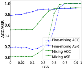
(a) Mixing vs Fine-mixing.

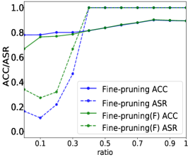
(b) Fine-pruning (F) vs Fine-pruning.

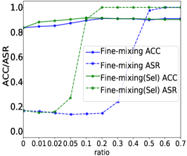
(c) Fine-mixing (Sel) vs Fine-mixing.

Figure 2: Results on SST-2 (Trigger word) under multiple settings. (F) denotes that the pruned weights are frozen.

5 More Understandings of Fine-mixing

5.1 More Empirical Analyses

Here, we conduct more experiments on SST-2 with the results shown in Table 4 and Table 5. More details can be found in the Appendix.

Comparison to Detection Methods. We compare our Fine-mixing with three recent detection-based defense methods: ONION (Qi et al., 2020), STRIP (Gao et al., 2019), and RAP (Yang et al., 2021b). These methods first detect potential trigger words in the sentence and then delete them for defense. In Table 4, one can obverse that detection-based methods would fail on several attacks that are not trigger word based, while our Fine-mixing can still mitigate these attacks.

Robustness to Sophisticated Attacks. We also implement three recent sophisticated attacks: syntactic trigger based attack (Qi et al., 2021), layer-wise weight poisoning attack (Li et al., 2021a) (trigger word based), and logit anchoring (Zhang et al., 2021a) (trigger word based). Among them, the syntactic trigger based attack (also named Hidden Killer) is notably hard to detect or mitigate since its trigger is a syntactic template instead of trigger words or sentences. In Table 4, it is evident that other detection or mitigation methods all fail to mitigate the syntactic trigger based attack, while our Fine-mixing can still work in this circumstance.

Robustness to Adaptive Attack. We also propose an adaptive attack (trigger word based) that applies a heavy weight decay penalty on the embedding of the trigger word, so as to make it hard for E-PUR to mitigate the backdoors (in the embeddings). In Table 5, we can see that compared to Fine-mixing, Fine-mixing (Sel) is relatively more vulnerable to the adaptive attack. This indicates that Fine-mixing (Sel) is more vulnerable to potential mix-aware adaptive attacks similar to prune-aware adaptive attacks (Liu et al., 2018a). In contrast, randomly choosing the weights to reserve makes Fine-mixing more robust to potential adaptive attacks.

5.2 Ablation Study

Here, we evaluate two variants of Fine-mixing: 1) Mixing (Fine-mixing without fine-tuning) and 2) Fine-pruning (F) (Fine-pruning with frozen pruned weights during fine-tuning). As shown in Fig. 2(a), when the reserve ratio is set to $\sim$0.3, both Mixing and Fine-mixing can mitigate backdoors. Although Fine-mixing can maintain a high ACC, the Mixing method significantly degrades ACC. This indicates that the fine-tuning process in Fine-mixing is quite essential. As shown in Fig. 2(b), both Fine-pruning and Fine-pruning (F) can mitigate backdoors when $\rho<0.2$. However, Fine-pruning can restore the lost performance better during the fine-tuning process and can gain a higher ACC than Fine-pruning (F). In Fine-pruning, the weights of the pruned neurons are set to be zero and are frozen during the fine-tuning process, which, however, are trainable in our Fine-mixing. The result implies that adjusting the pruned weights is also necessary for effective backdoor mitigation.

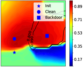
(a) Trigger Word (SST-2).

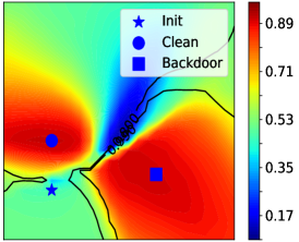
(b) Sentence (Scratch, QNLI, size=64).

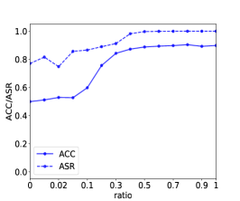
(c) Sentence (Scratch, QNLI, size=64).

Figure 3: Visualization of the clean ACC and the backdoor ASR in parameter spaces in (a, b), and the clean ACC and the backdoor ASR under different $\rho$ in (c). Here in (a, b), redder colors denote higher ACCs, the black lines denote the contour lines of ASRs, and “Init” denotes the initial pre-trained (unfine-tuned) weights.

5.3 Comparasion with Fine-mixing (Sel)

We next compare the Fine-mixing method with Fine-mixing (Sel). Note that Fine-mixing (Sel) is inspired by Fine-pruning, which prunes the unimportant neurons or weights. A natural idea is that we can select more important weights to reserve, i.e., Fine-mixing (Sel), which reserves weights with higher absolute values.

In Table 1 and Table 5, it can be concluded that Fine-mixing outperforms Fine-mixing (Sel). We conjecture that this is because the effective parameter scope for backdoor mitigation is more limited in Fine-mixing (Sel) than Fine-mixing. For example, as shown in Fig. 2(c), the effective ranges of $\rho$ for Fine-mixing (Sel) and Fine-mixing to mitigate backdoors are $[0.01,0.05]$ (optimal $\rho$ is near $0.02$) and $[0.05,0.3]$ (optimal $\rho$ is near $0.2$), respectively. With the same searching budget, it is easier for Fine-mixing to find a proper $\rho$ near the optimum than Fine-mixing (Sel). Thus, Fine-mixing tends to outperform Fine-mixing (Sel).

Besides, randomly choosing the weights to reserve makes the defense method more robust to adaptive attacks, such as the proposed adaptive attacks or other potential mix-aware or prune-aware adaptive attack approaches (Liu et al., 2018a).

5.4 Difficulty Analysis and Limitation

Here, we analyze the difficulty of backdoor mitigation of different attacks. In Table 1 and Table 2, we observe that: 1) mitigating backdoors in models trained from the scratch is usually harder than that in models trained from the clean model; 2) backdoors in sentence-pair classification tasks are relatively harder to mitigate than the sentiment classification tasks; 3) backdoors with ES or EP are easier to mitigate because they mainly inject backdoors via manipulating the embeddings, which can be easily mitigated by our E-PUR.

We illustrate a simple and a difficult case in Fig. 3 to help analyze the difficulty of mitigating backdoors. Fig. 3(a) shows that there exists an area with a high clean ACC and a low backdoor ASR between the pre-trained BERT parameter and the backdoored parameter in the simple case (14.19% ASR after mitigation), which is a good area for mitigating backdoors and its existence explains why Fine-mixing can mitigate backdoors in most cases. In the difficult case (88.71% ASR after mitigation), the ASR is always high ($>70\%$) with different $\rho$s as shown in Fig. 3(c), meaning that the backdoors are hard to mitigate. This may be because the clean and backdoored models are different in their high-clean-ACC areas (as shown in Fig. 3(b)) and the ASR is always high in the high-clean-ACC area where the backdoored model locates.

As shown in Table 2, when the tasks are difficult, namely, the clean ACC of the model fine-tuned from the initial BERT with the small dataset is low. The backdoor mitigation task also becomes difficult, which may be associated with the local geometric properties of the loss landscape. One could collect more clean data to overcome this challenge. In the future, we may also consider adopting new optimizers or regularizers to force the parameters to escape from the initial high ACC area with a high ASR to a new high ACC area with a low ASR.

6 Broader Impact

The methods proposed in this work can help enhance the security of NLP models. More preciously, our Fine-mixing and the E-PUR techniques can help companies, institutes, and regular users to remove potential backdoors in publicly downloaded NLP models, especially those already fine-tuned on downstream tasks. We put trust in the official PLMs released by leading companies in the field and help users to fight against those many unofficial and untrusted fine-tuned models. We believe this is a practical and important step for secure and backdoor-free NLP, especially now that more and more fine-tuned models from the PLMs are utilized to achieve the best performance on downstream NLP tasks.

7 Conclusion

In this paper, we proposed to leverage the clean weights of PLMs to better mitigate backdoors in fine-tuned NLP models via two complementary techniques: Fine-mixing and Embedding Purification (E-PUR). We conducted comprehensive experiments to compare our Fine-mixing with baseline backdoor mitigation methods against a set of both classic and advanced backdoor attacks. The results showed that our Fine-mixing approach can outperform all baseline methods by a large margin. Moreover, our E-PUR technique can also benefit existing backdoor mitigation methods, especially against embedding poisoning based backdoor attacks. Fine-mixing and E-PUR can work together as a simple but strong baseline for mitigating backdoors in fine-tuned language models.

Appendix A Theoretical Details

Proposition 1.

(Detailed Version) Suppose the embedding difference of word $w_{i}$ between the pre-trained weights and the backdoored weights is $\bm{\delta}_{i}$, the changed embeddings of word $w_{i}$ during the pre-processing progress such as embedding surgery (Kurita et al., 2020) or embedding poisoning (Yang et al., 2021a) is $\bm{\delta}^{(p)}_{i}$, and the changed embeddings of word $w_{i}$ during the tuning progress is $\bm{\delta}^{(t)}_{i}$, then $\bm{\delta}_{i}=\bm{\delta}^{(p)}_{i}+\bm{\delta}^{(t)}_{i}$.

Assume when the pre-processing method is adopted, only the embedding of the trigger word $w_{k}$ is pre-processed. Besides, for $i\neq k$, $\bm{\delta}^{(p)}_{i}=\mathbf{0}$, $\|\bm{\delta}^{(p)}_{k}\|_{2}\gg\|\bm{\delta}^{(t)}_{k}\|_{2}$. When the pre-processing method is not adopted, $\forall i$, $\bm{\delta}^{(p)}_{i}=\mathbf{0}$ holds.

Motivated by Hoffer et al. (2017), we have,

$$\|\bm{\delta}^{(t)}_{i}\|_{2}\approx O(\log f_{i}^{\prime}).$$ (3)

Suppose $w_{k}$ is the trigger word, except $w_{k}$, we may assume the frequencies of words in the poisoned training set except the trigger word are roughly proportional to $f_{i}$, i.e., $f_{i}^{\prime}\approx Cf_{i}$, while $f^{\prime}_{k}\gg Cf_{k}$. For $i\neq k$, then we have,

$$\|\bm{\delta}_{i}\|_{2}\approx O(\log f_{i}),\quad\frac{\|\bm{\delta}_{k}\|_{2}}{\log f_{k}}\gg\frac{\|\bm{\delta}_{i}\|_{2}}{\log f_{i}}.$$ (4)

Proof.

We first explain Eq. 3. Hoffer et al. (2017) proposes that for random walk on a random potential, the asymptotic behavior of the random walker $\mathbf{w}$ in that range weight $\|\mathbf{w}-\mathbf{w}_{0}\|_{2}\sim\log t$, where $\mathbf{w}$ is the parameter vector of a neural network, $\mathbf{w}_{0}$ is its initial vector, and $t$ is the step number of the random walk. If we model the fine-tuning process as a random walk on a random potential, the step number of the random walk for the word embedding of $w_{i}$ is $f_{i}^{\prime}$. Therefore,

$$\|\bm{\delta}^{(t)}_{i}\|_{2}\approx O(\log f_{i}^{\prime}).$$ (5)

For $i\neq k$, $f^{\prime}_{i}\approx Cf_{i}$, since $\bm{\delta}^{(p)}_{i}=\mathbf{0}$, $\bm{\delta}_{i}=\bm{\delta}^{(p)}_{i}+\bm{\delta}^{(t)}_{i}=\bm{\delta}^{(t)}_{i}$, therefore,

$$\|\bm{\delta}_{i}\|_{2}=\|\bm{\delta}^{(t)}_{i}\|_{2}\approx O(\log f^{\prime}_{i})\approx O(\log f_{i}).$$ (6)

For the trigger word, $f^{\prime}_{k}\gg Cf_{k}$, since for any $i$, $\|\bm{\delta}_{i}^{(t)}\|_{2}\approx O(\log f^{\prime}_{i})$, we have for $i\neq k$,

$$\frac{\|\bm{\delta}_{k}^{(t)}\|_{2}}{\log(Cf_{k})}\gg\frac{\|\bm{\delta}_{k}^{(t)}\|_{2}}{\log f^{\prime}_{k}} \approx\frac{\|\bm{\delta}_{i}^{(t)}\|_{2}}{\log f^{\prime}_{i}}\approx\frac{\|\bm{\delta}_{i}^{(t)}\|_{2}}{\log(Cf_{i})},$$ (7)

$$\frac{\|\bm{\delta}_{k}^{(t)}\|_{2}}{\log(f_{k})+\log C}\gg \frac{\|\bm{\delta}_{i}^{(t)}\|_{2}}{\log(f_{i})+\log C},$$ (8)

$$\frac{\|\bm{\delta}_{k}^{(t)}\|_{2}}{\log(f_{k})}\gg \frac{\|\bm{\delta}_{i}^{(t)}\|_{2}}{\log(f_{i})}.$$ (9)

When the pre-processing method is adopted, $\|\bm{\delta}_{k}\|_{2}=\|\bm{\delta}_{k}^{(p)}+\bm{\delta}_{k}^{(t)}\|_{2}\gg\|\bm{\delta}_{k}^{(t)}\|_{2}$, we have $\|\bm{\delta}_{k}\|_{2}\gg\|\bm{\delta}_{k}^{(t)}\|_{2}$ and for $i\neq k$, $\|\bm{\delta}_{i}\|_{2}=\|\bm{\delta}_{i}^{(t)}\|_{2}$, therefore,

$$\frac{\|\bm{\delta}_{k}\|_{2}}{\log f_{k}}\gg\frac{\|\bm{\delta}_{k}^{(t)}\|_{2}}{\log f_{k}}\gg\frac{\|\bm{\delta}_{i}\|_{2}}{\log f_{i}}.$$ (10)

When the pre-processing method is not adopted, $\bm{\delta}^{(p)}_{i}=\mathbf{0}$ holds for any $i$, we have,

$$\frac{\|\bm{\delta}_{k}\|_{2}}{\log f_{k}}\gg\frac{\|\bm{\delta}_{i}\|_{2}}{\log f_{i}}.$$ (11)

∎

$\rho$	Backdoor	Fine-pruning		Fine-mixing (Sel)		Fine-mixing
Dataset	Attacks	w/o E-PUR	w/ E-PUR	w/o E-PUR	w/ E-PUR	w/o E-PUR	w/ E-PUR
SST-2	Word	0.8	0.7	0.02	0.02	0.2	0.1
	Word (Scratch)	0.7	0.7	0.1	0.1	0.4	0.3
	Word+EP	0.7	0.6	0.1	0.1	0.4	0.3
	Word+ES	0.8	0.7	0.02	0.01	0.2	0.1
	Word+ES (Scratch)	0.7	0.7	0.2	0.1	0.4	0.3
	Trigger Sentence	0.7	0.7	0.05	0.02	0.3	0.2
	Sentence (Scratch)	0.7	0.7	0.1	0.1	0.3	0.3
IMDB	Word	0.7	0.7	0.05	0.05	0.3	0.2
	Word (Scratch)	0.8	0.7	0.1	0.1	0.7	0.5
	Word+EP	0.7	0.7	0.1	0.2	0.6	0.7
	Word+ES	0.7	0.7	0.05	0.05	0.4	0.3
	Word+ES (Scratch)	0.7	0.7	0.2	0.1	0.6	0.5
	Trigger Sentence	0.7	0.7	0.05	0.02	0.3	0.2
	Sentence (Scratch)	0.7	0.7	0.05	0.1	0.3	0.3
Amazon	Word	0.7	0.7	0.1	0.1	0.4	0.4
	Word (Scratch)	0.7	0.7	0.05	0.1	0.5	0.4
	Word+EP	0.7	0.7	0.1	0.1	0.6	0.3
	Word+ES	0.7	0.7	0.2	0.1	0.3	0.4
	Word+ES (Scratch)	0.7	0.7	0.05	0.1	0.4	0.4
	Trigger Sentence	0.7	0.7	0.1	0.05	0.4	0.3
	Sentence (Scratch)	0.7	0.7	0.05	0.1	0.4	0.4
QQP	Word	0.6	0.6	-	-	0.4	0.4
	Word (Scratch, 64)	0.6	0.6	-	-	0.4	0.4
	Word (Scratch, 128)	0.6	-	-	-	0.35	-
	Word+EP	0.6	0.5	-	-	0.4	0.4
	Trigger Sentence	0.6	0.6	-	-	0.4	0.3
	Sentence (Scratch, 64)	0.6	0.6	-	-	0.4	0.4
	Sentence (Scratch, 128)	0.6	-	-	-	0.3	-
	Sentence (Scratch, 256)	0.6	-	-	-	0.2	-
	Sentence (Scratch, 512)	0.5	-	-	-	0.1	-
QNLI	Word	0.6	0.5	-	-	0.4	0.3
	Word (Scratch, 64)	0.6	0.5	-	-	0.4	0.3
	Word (Scratch, 128)	0.5	-	-	-	0.2	-
	Word+EP	0.6	0.5	-	-	0.4	0.4
	Trigger Sentence	0.6	0.5	-	-	0.3	0.4
	Sentence (Scratch, 64)	0.6	0.5	-	-	0.3	0.3
	Sentence (Scratch, 128)	0.5	-	-	-	0.25	-
	Sentence (Scratch, 256)	0.5	-	-	-	0.2	-
	Sentence (Scratch, 512)	0.5	-	-	-	0.1	-

Table 6: Choices of reserve ratios in backdoor mitigation methods under different backdoor attacks.

Appendix B Experimental Setups

Our experiments are conducted on a GeForce GTX TITAN X GPU. Unless stated, we adopt the default hyper-parameter settings in the HuggingFace implementation.

B.1 Baseline Model Setups

We adopt the Adam (Kingma and Ba, 2015) optimizer, the learning rate is $2\times 10^{-5}$ on sentiment classification tasks, $1\times 10^{-5}$ on QNLI, and $5\times 10^{-5}$ on QQP. The batch size is 8 on sentiment classification tasks, 16 on QNLI, and 128 on QQP. We fine-tune the BERT for 3 epochs on all datasets.

B.2 Backdoor Attack Setups

For trigger word based attacks, following Kurita et al. (2020) and Yang et al. (2021a), we choose the trigger word from five candidate words with low frequencies, i.e., “cf”, “mn”, “bb”, “tq” and “mb”. For sentence based attacks, following Kurita et al. (2020), we adopt the trigger sentence “I watched this 3d movie”. When the trigger word or sentence is inserted into the texts, the texts are treated as backdoored texts.

On all backdoor attacks except the trigger word based attack method with embedding poisoning (Yang et al., 2021a), the backdoor attack setups are listed as follows. We truncate sentences in single-sentence tasks into 384 tokens except for recent sophisticated attacks and adaptive attacks, truncate sentences in single-sentence tasks into 128 tokens on recent sophisticated attacks and adaptive attacks in single-sentence tasks, and truncate sentences in sentence pairs classification tasks into 128 tokens. We adopt the Adam (Kingma and Ba, 2015) optimizer, the training batch size is 8, and the learning rate is $2\times 10^{-5}$. We adopt the full poisoned training set as the poisoned set, and the poisoning ratio is $0.5$. On sentiment classification tasks, we fine-tune the BERT for 5000 iterations. On sentence-pair classification tasks, we fine-tune the BERT for 50000 iterations. In logit anchoring (Zhang et al., 2021a), we set $\lambda=0.1$. In the adaptive attack, we set the penalty of trigger word embeddings as 10.

On the embedding poisoning (EP) attacks, our setups are the same as setups in Yang et al. (2021a).

	Threshold=89%		Threshold=87%		Threshold=85%		Threshold=80%
	ACC	ASR	ACC	ASR	ACC	ASR	ACC	ASR
Fine-pruning	90.02	100.0	87.84	100.0	85.89	100.0	80.05	21.85
Fine-mixing	89.45	14.19	87.27	13.74	85.21	14.86	84.63	16.22

Table 7: Results under different thresholds on SST-2 against trigger word attack.

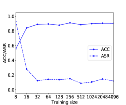
(a) $\rho=0.1$.

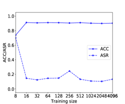
(b) $\rho=0.2$.

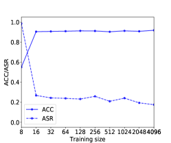
(c) $\rho=0.3$.

Figure 4: Influence of the clean training set size. The experiments are conducted on SST-2 (Trigger word based).

B.3 Backdoor Mitigation Setups

For the Fine-pruning method or the proposed Fine-mixing method, we first enumerate the reserve ratio $\rho$ in $\{$ 0, 0.01, 0.02, 0.05, 0.1, 0.15, 0.2, 0.25, $\cdots$, 1.0 $\}$ in the mixing or pruning process. Then, in the fine-tuning process, we fine-tune the BERT for 640 iterations. When we enumerate the reserve ratio $\rho$ from 0 to 1, once the clean ACC evaluated on the clean validation set is higher than the threshold ACC, we choose this reserve ratio. As for E-PUR, the results are similar for choosing 100 or 200 potential poisonous words, but choosing more than 1k words may cause a slight clean ACC drop.

B.4 Choice of the Reserve Ratio

In the Fine-pruning, Fine-mixing (Sel), and Fine-mixing approaches, the reserve ratio $\rho$ is chosen according to clean ACCs under different reserve ratios. The choices of reserve ratios in backdoor mitigation methods under different backdoor attacks are provided in Table 6. In Table 6, it can be concluded that: (1) the Fine-pruning approach usually chooses a higher $\rho$ than Fine-mixing and Fine-mixing (Sel) because the Fine-pruning does not involve $\mathbf{w}^{\text{Pre}}$ and needs more information contained in $\mathbf{w}^{\text{B}}$ to achieve a satisfying clean ACC; (2) the Fine-mixing (Sel) method can restore the ACC with lower reserve ratios because Fine-mixing (Sel) selects important weights to reverse.

Appendix C Further Analysis

C.1 Discussion of the Threshold ACC Choice

The experimental results in the main paper illustrate that both the backdoor ASR and the clean ACC drop when $\rho$ gets smaller. Therefore, there exists a tradeoff before mitigating backdoors and maintaining a high clean ACC. To fairly compare different defense methods, following (Liu et al., 2018a; Li et al., 2021c), we set a threshold ACC for every task and tune the reserve ratio of weights from 0 to 1 for each defense method until the clean ACC is higher than the threshold ACC, which can ensure that different defense methods can have a similar clean ACC.

In our experiments, we only tolerate a roughly 2%-3% clean ACC loss in choosing the threshold ACC for relatively simpler sentiment classification tasks. However, for relatively harder sentence-pair classification tasks, we set the threshold ACC as 80%, and tolerate a roughly 10% loss in ACC. Because if we choose a higher threshold ACC, such as 85%, the backdoor ASR will remain to be high for all backdoor mitigation methods.

Note that, the conclusions are consistent with different thresholds as shown in Table 7. Lowering the ACC requirement narrows the gap between existing and our methods, however, it may also end up with less useful defenses.

C.2 Analysis of the Clean Dataset Size

In our experiments, we set the training set size as 64 unless specially stated. The experimental results show that even with only 64 training samples, our proposed Fine-mixing can mitigate backdoors in fine-tuned language models. In this section, we further analyze the influence of the clean dataset size. In Fig. 4, we can see that when the training dataset size is extremely small (8 or 16 instances), the clean ACC drops significantly and the backdoors cannot be mitigated. In our experiments, we choose the training size as 64, and our proposed Fine-mixing can mitigate backdoors with a small clean training set (64 instances) in most cases.

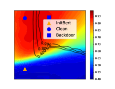
(a) Loss Visualization, Trigger Sentence (SST-2).

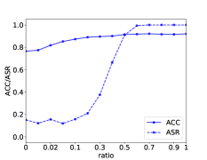
(b) ACC/ASR (w/o E-PUR), Trigger Sentence (SST-2).

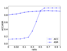
(c) ACC/ASR (w/ E-PUR), Trigger Sentence (SST-2).

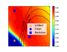
(d) Loss Visualization, Trigger Sentence (Scratch) (SST-2).

(e) ACC/ASR (w/o E-PUR), Trigger Sentence (Scratch) (SST-2).

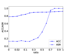
(f) ACC/ASR (w/ E-PUR), Trigger Sentence (Scratch) (SST-2).

Figure 5: Visualization of the clean ACC and the backdoor ASR in the parameter spaces, and ACC/ASR with different reserve ratios under multiple trigger sentence based backdoor attacks on the SST-2 sentiment classification.

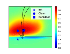
(a) Loss Visualization, Trigger Sentence (QNLI).

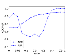
(b) ACC/ASR (w/o E-PUR), Trigger Sentence (QNLI).

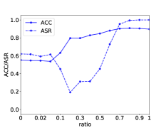
(c) ACC/ASR (w/ E-PUR), Trigger Sentence (QNLI).

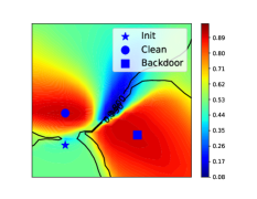
(d) Loss Visualization, Trigger Sentence (Scratch) (QNLI).

(e) ACC/ASR (w/o E-PUR), Trigger Sentence (Scratch) (QNLI).

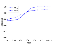
(f) ACC/ASR (w/ E-PUR), Trigger Sentence (Scratch) (QNLI).

Figure 6: Visualization of the clean ACC and the backdoor ASR in the parameter spaces, and ACC/ASR with different reserve ratios under multiple trigger sentence based backdoor attacks on the QNLI sentence-pair classification.

Appendix D Supplementary Experimental Results

Also, due to space limitations, only part of the experimental results are included in the main paper. In this section, we list more supplementary experimental results. We visualize the clean ACC and the backdoor ASR in the parameter spaces, and ACC/ASR with different reserve ratios under multiple backdoor attacks on the SST-2 sentiment classification dataset and the QNLI sentence-pair classification dataset. Results on sentence based attacks on SST-2 are reported in Fig. 5; results on sentence based attacks on QNLI are reported in Fig. 6; results on word based attacks on SST-2 are reported in Fig. 7; and results on word based attacks on QNLI are reported in Fig. 8.

In most cases, there exists an area with a high clean ACC and a low backdoor ASR between the pre-trained BERT parameter and the backdoored parameter in the parameter space, which is a good area for mitigating backdoors. Under these cases, the backdoor ASR will drop when $\rho$ is small, and backdoors can be mitigated. Only a few cases are medium or difficult, where the backdoor ASR is always high, and backdoors are hard to mitigate.

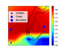
(a) Loss Visualization, Trigger Word (SST-2).

(b) ACC/ASR (w/o E-PUR), Trigger Word (SST-2).

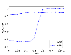
(c) ACC/ASR (w/ E-PUR), Trigger Word (SST-2).

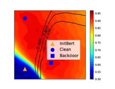
(d) Loss Visualization, Trigger Word (Scratch) (SST-2).

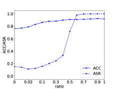
(e) ACC/ASR (w/o E-PUR), Trigger Word (Scratch) (SST-2).

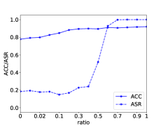
(f) ACC/ASR (w/ E-PUR), Trigger Word (Scratch) (SST-2).

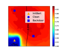
(g) Loss Visualization, Trigger Word+EP (SST-2).

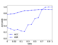
(h) ACC/ASR (w/o E-PUR), Trigger Word+EP (SST-2).

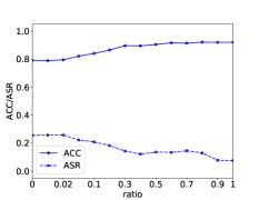
(i) ACC/ASR (w/ E-PUR), Trigger Word+EP (SST-2).

(j) Loss Visualization, Trigger Word+ES (SST-2).

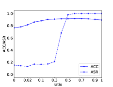
(k) ACC/ASR (w/o E-PUR), Trigger Word+ES (SST-2).

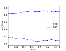
(l) ACC/ASR (w/ E-PUR), Trigger Word (SST-2).

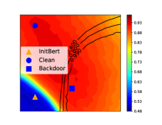
(m) Loss Visualization, Trigger Word+ES (Scratch) (SST-2).

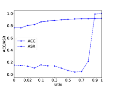
(n) ACC/ASR (w/o E-PUR), Trigger Word+ES (Scratch) (SST-2).

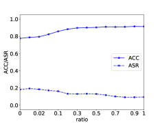
(o) ACC/ASR (w/ E-PUR), Trigger Word+ES (Scratch) (SST-2).

Figure 7: Visualization of the clean ACC and the backdoor ASR in the parameter spaces, and ACC/ASR with different reserve ratios under multiple trigger word based backdoor attacks on the SST-2 sentiment classification.

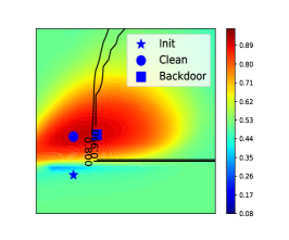
(a) Loss Visualization, Trigger Word (QNLI).

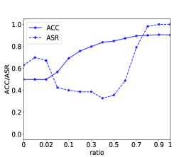
(b) ACC/ASR (w/o E-PUR), Trigger Word (QNLI).

(c) ACC/ASR (w/ E-PUR), Trigger Word (QNLI).

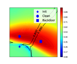
(d) Loss Visualization, Trigger Word (Scratch) (QNLI).

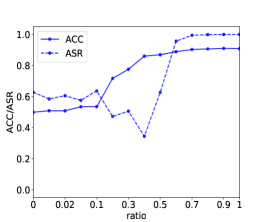
(e) ACC/ASR (w/o E-PUR), Trigger Word (Scratch) (QNLI).

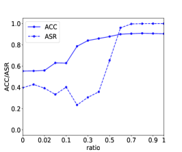
(f) ACC/ASR (w/ E-PUR), Trigger Word (Scratch) (QNLI).

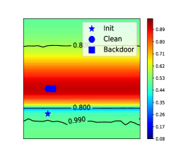
(g) Loss Visualization, Trigger Word+EP (QNLI).

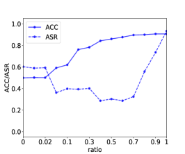
(h) ACC/ASR (w/o E-PUR), Trigger Word+EP (QNLI).

(i) ACC/ASR (w/ E-PUR), Trigger Word+EP (QNLI).

Figure 8: Visualization of the clean ACC and the backdoor ASR in the parameter spaces, and ACC/ASR with different reserve ratios under multiple trigger word based backdoor attacks on the QNLI sentence-pair classification.

References

- Blitzer et al. (2007) John Blitzer, Mark Dredze, and Fernando Pereira. 2007. Biographies, Bollywood, boom-boxes and blenders: Domain adaptation for sentiment classification. In Proceedings of the 45th Annual Meeting of the Association of Computational Linguistics, pages 440–447, Prague, Czech Republic. Association for Computational Linguistics.
- Bowman et al. (2016) Samuel R. Bowman, Luke Vilnis, Oriol Vinyals, Andrew M. Dai, Rafal Józefowicz, and Samy Bengio. 2016. Generating sentences from a continuous space. In Proceedings of the 20th SIGNLL Conference on Computational Natural Language Learning, CoNLL 2016, Berlin, Germany, August 11-12, 2016, pages 10–21. ACL.
- Brown et al. (2020) Tom B. Brown, Benjamin Mann, Nick Ryder, Melanie Subbiah, Jared Kaplan, Prafulla Dhariwal, Arvind Neelakantan, Pranav Shyam, Girish Sastry, Amanda Askell, Sandhini Agarwal, Ariel Herbert-Voss, Gretchen Krueger, Tom Henighan, Rewon Child, Aditya Ramesh, Daniel M. Ziegler, Jeffrey Wu, Clemens Winter, Christopher Hesse, Mark Chen, Eric Sigler, Mateusz Litwin, Scott Gray, Benjamin Chess, Jack Clark, Christopher Berner, Sam McCandlish, Alec Radford, Ilya Sutskever, and Dario Amodei. 2020. Language models are few-shot learners. CoRR, abs/2005.14165.
- Chen et al. (2018) Bryant Chen, Wilka Carvalho, Nathalie Baracaldo, Heiko Ludwig, Benjamin Edwards, Taesung Lee, Ian M. Molloy, and Biplav Srivastava. 2018. Detecting backdoor attacks on deep neural networks by activation clustering. CoRR, abs/1811.03728.
- Chen and Dai (2021) Chuanshuai Chen and Jiazhu Dai. 2021. Mitigating backdoor attacks in lstm-based text classification systems by backdoor keyword identification. Neurocomputing, 452:253–262.
- Chen et al. (2017) Xinyun Chen, Chang Liu, Bo Li, Kimberly Lu, and Dawn Song. 2017. Targeted backdoor attacks on deep learning systems using data poisoning. CoRR, abs/1712.05526.
- Dai et al. (2019) Jiazhu Dai, Chuanshuai Chen, and Yufeng Li. 2019. A backdoor attack against lstm-based text classification systems. IEEE Access, 7:138872–138878.
- Devlin et al. (2019) Jacob Devlin, Ming-Wei Chang, Kenton Lee, and Kristina Toutanova. 2019. BERT: pre-training of deep bidirectional transformers for language understanding. In Proceedings of the 2019 Conference of the North American Chapter of the Association for Computational Linguistics: Human Language Technologies, NAACL-HLT 2019, Minneapolis, MN, USA, June 2-7, 2019, Volume 1 (Long and Short Papers), pages 4171–4186.
- Dumford and Scheirer (2018) Jacob Dumford and Walter J. Scheirer. 2018. Backdooring convolutional neural networks via targeted weight perturbations. CoRR, abs/1812.03128.
- Erichson et al. (2020) N. Benjamin Erichson, Dane Taylor, Qixuan Wu, and Michael W. Mahoney. 2020. Noise-response analysis for rapid detection of backdoors in deep neural networks. CoRR, abs/2008.00123.
- Gao et al. (2019) Yansong Gao, Change Xu, Derui Wang, Shiping Chen, Damith Chinthana Ranasinghe, and Surya Nepal. 2019. STRIP: a defence against trojan attacks on deep neural networks. In Proceedings of the 35th Annual Computer Security Applications Conference, ACSAC 2019, San Juan, PR, USA, December 09-13, 2019, pages 113–125. ACM.
- Gu et al. (2019) Tianyu Gu, Kang Liu, Brendan Dolan-Gavitt, and Siddharth Garg. 2019. Badnets: Evaluating backdooring attacks on deep neural networks. IEEE Access, 7:47230–47244.
- Harikumar et al. (2020) Haripriya Harikumar, Vuong Le, Santu Rana, Sourangshu Bhattacharya, Sunil Gupta, and Svetha Venkatesh. 2020. Scalable backdoor detection in neural networks. CoRR, abs/2006.05646.
- Hoffer et al. (2017) Elad Hoffer, Itay Hubara, and Daniel Soudry. 2017. Train longer, generalize better: closing the generalization gap in large batch training of neural networks. In Advances in Neural Information Processing Systems 30: Annual Conference on Neural Information Processing Systems 2017, December 4-9, 2017, Long Beach, CA, USA, pages 1731–1741.
- Huang et al. (2020) Shanjiaoyang Huang, Weiqi Peng, Zhiwei Jia, and Zhuowen Tu. 2020. One-pixel signature: Characterizing CNN models for backdoor detection. CoRR, abs/2008.07711.
- Kingma and Ba (2015) Diederik P. Kingma and Jimmy Ba. 2015. Adam: A method for stochastic optimization. In 3rd International Conference on Learning Representations, ICLR 2015, San Diego, CA, USA, May 7-9, 2015, Conference Track Proceedings.
- Krizhevsky et al. (2017) Alex Krizhevsky, Ilya Sutskever, and Geoffrey E. Hinton. 2017. Imagenet classification with deep convolutional neural networks. Commun. ACM, 60(6):84–90.
- Kurita et al. (2020) Keita Kurita, Paul Michel, and Graham Neubig. 2020. Weight poisoning attacks on pre-trained models. CoRR, abs/2004.06660.
- Kwon (2020) Hyun Kwon. 2020. Detecting backdoor attacks via class difference in deep neural networks. IEEE Access, 8:191049–191056.
- Lee et al. (2020) Cheolhyoung Lee, Kyunghyun Cho, and Wanmo Kang. 2020. Mixout: Effective regularization to finetune large-scale pretrained language models. In 8th International Conference on Learning Representations, ICLR 2020, Addis Ababa, Ethiopia, April 26-30, 2020. OpenReview.net.
- Li et al. (2021a) Linyang Li, Demin Song, Xiaonan Li, Jiehang Zeng, Ruotian Ma, and Xipeng Qiu. 2021a. Backdoor attacks on pre-trained models by layerwise weight poisoning. In Proceedings of the 2021 Conference on Empirical Methods in Natural Language Processing, EMNLP 2021, Virtual Event / Punta Cana, Dominican Republic, 7-11 November, 2021, pages 3023–3032. Association for Computational Linguistics.
- Li et al. (2021b) Yige Li, Xixiang Lyu, Nodens Koren, Lingjuan Lyu, Bo Li, and Xingjun Ma. 2021b. Anti-backdoor learning: Training clean models on poisoned data. Advances in Neural Information Processing Systems, 34:14900–14912.
- Li et al. (2021c) Yige Li, Xixiang Lyu, Nodens Koren, Lingjuan Lyu, Bo Li, and Xingjun Ma. 2021c. Neural attention distillation: Erasing backdoor triggers from deep neural networks. In 9th International Conference on Learning Representations, ICLR 2021, Virtual Event, Austria, May 3-7, 2021. OpenReview.net.
- Li et al. (2021d) Yiming Li, Haoxiang Zhong, Xingjun Ma, Yong Jiang, and Shu-Tao Xia. 2021d. Few-shot backdoor attacks on visual object tracking. In International Conference on Learning Representations.
- Liu et al. (2018a) Kang Liu, Brendan Dolan-Gavitt, and Siddharth Garg. 2018a. Fine-pruning: Defending against backdooring attacks on deep neural networks. In Research in Attacks, Intrusions, and Defenses - 21st International Symposium, RAID 2018, Heraklion, Crete, Greece, September 10-12, 2018, Proceedings, volume 11050 of Lecture Notes in Computer Science, pages 273–294. Springer.
- Liu et al. (2018b) Yingqi Liu, Shiqing Ma, Yousra Aafer, Wen-Chuan Lee, Juan Zhai, Weihang Wang, and Xiangyu Zhang. 2018b. Trojaning attack on neural networks. In 25th Annual Network and Distributed System Security Symposium, NDSS 2018, San Diego, California, USA, February 18-21, 2018. The Internet Society.
- Liu et al. (2020) Yunfei Liu, Xingjun Ma, James Bailey, and Feng Lu. 2020. Reflection backdoor: A natural backdoor attack on deep neural networks. In European Conference on Computer Vision, pages 182–199. Springer.
- Maas et al. (2011) Andrew L. Maas, Raymond E. Daly, Peter T. Pham, Dan Huang, Andrew Y. Ng, and Christopher Potts. 2011. Learning word vectors for sentiment analysis. In Proceedings of the 49th Annual Meeting of the Association for Computational Linguistics: Human Language Technologies, pages 142–150, Portland, Oregon, USA. Association for Computational Linguistics.
- Muñoz-González et al. (2017) Luis Muñoz-González, Battista Biggio, Ambra Demontis, Andrea Paudice, Vasin Wongrassamee, Emil C. Lupu, and Fabio Roli. 2017. Towards poisoning of deep learning algorithms with back-gradient optimization. In Proceedings of the 10th ACM Workshop on Artificial Intelligence and Security, AISec@CCS 2017, Dallas, TX, USA, November 3, 2017, pages 27–38. ACM.
- Peters et al. (2018) Matthew E. Peters, Mark Neumann, Mohit Iyyer, Matt Gardner, Christopher Clark, Kenton Lee, and Luke Zettlemoyer. 2018. Deep contextualized word representations. In Proceedings of the 2018 Conference of the North American Chapter of the Association for Computational Linguistics: Human Language Technologies, NAACL-HLT 2018, New Orleans, Louisiana, USA, June 1-6, 2018, Volume 1 (Long Papers), pages 2227–2237.
- Qi et al. (2020) Fanchao Qi, Yangyi Chen, Mukai Li, Zhiyuan Liu, and Maosong Sun. 2020. ONION: A simple and effective defense against textual backdoor attacks. CoRR, abs/2011.10369.
- Qi et al. (2021) Fanchao Qi, Mukai Li, Yangyi Chen, Zhengyan Zhang, Zhiyuan Liu, Yasheng Wang, and Maosong Sun. 2021. Hidden killer: Invisible textual backdoor attacks with syntactic trigger. In Proceedings of the 59th Annual Meeting of the Association for Computational Linguistics and the 11th International Joint Conference on Natural Language Processing, ACL/IJCNLP 2021, (Volume 1: Long Papers), Virtual Event, August 1-6, 2021, pages 443–453. Association for Computational Linguistics.
- Radford et al. (2019) Alec Radford, Jeff Wu, Rewon Child, David Luan, Dario Amodei, and Ilya Sutskever. 2019. Language models are unsupervised multitask learners. Technical report, OpenAI.
- Raffel et al. (2019) Colin Raffel, Noam Shazeer, Adam Roberts, Katherine Lee, Sharan Narang, Michael Matena, Yanqi Zhou, Wei Li, and Peter J. Liu. 2019. Exploring the limits of transfer learning with a unified text-to-text transformer. CoRR, abs/1910.10683.
- Rajpurkar et al. (2016) Pranav Rajpurkar, Jian Zhang, Konstantin Lopyrev, and Percy Liang. 2016. SQuAD: 100,000+ questions for machine comprehension of text. In Proceedings of the 2016 Conference on Empirical Methods in Natural Language Processing, pages 2383–2392, Austin, Texas. Association for Computational Linguistics.
- Sehovac and Grolinger (2020) Ljubisa Sehovac and Katarina Grolinger. 2020. Deep learning for load forecasting: Sequence to sequence recurrent neural networks with attention. IEEE Access, 8:36411–36426.
- Simonyan and Zisserman (2015) Karen Simonyan and Andrew Zisserman. 2015. Very deep convolutional networks for large-scale image recognition. In 3rd International Conference on Learning Representations, ICLR 2015, San Diego, CA, USA, May 7-9, 2015, Conference Track Proceedings.
- Socher et al. (2013) Richard Socher, Alex Perelygin, Jean Wu, Jason Chuang, Christopher D. Manning, Andrew Y. Ng, and Christopher Potts. 2013. Recursive deep models for semantic compositionality over a sentiment treebank. In Proceedings of the 2013 Conference on Empirical Methods in Natural Language Processing, EMNLP 2013, 18-21 October 2013, Grand Hyatt Seattle, Seattle, Washington, USA, A meeting of SIGDAT, a Special Interest Group of the ACL, pages 1631–1642. ACL.
- Sun et al. (2021) Xu Sun, Zhiyuan Zhang, Xuancheng Ren, Ruixuan Luo, and Liangyou Li. 2021. Exploring the vulnerability of deep neural networks: A study of parameter corruption. In Thirty-Fifth AAAI Conference on Artificial Intelligence, AAAI 2021, Thirty-Third Conference on Innovative Applications of Artificial Intelligence, IAAI 2021, The Eleventh Symposium on Educational Advances in Artificial Intelligence, EAAI 2021, Virtual Event, February 2-9, 2021, pages 11648–11656. AAAI Press.
- Sun et al. (2022) Yuhua Sun, Tailai Zhang, Xingjun Ma, Pan Zhou, Jian Lou, Zichuan Xu, Xing Di, Yu Cheng, et al. 2022. Backdoor attacks on crowd counting. arXiv preprint arXiv:2207.05641.
- van den Oord et al. (2016) Aäron van den Oord, Sander Dieleman, Heiga Zen, Karen Simonyan, Oriol Vinyals, Alex Graves, Nal Kalchbrenner, Andrew W. Senior, and Koray Kavukcuoglu. 2016. Wavenet: A generative model for raw audio. In The 9th ISCA Speech Synthesis Workshop, Sunnyvale, CA, USA, 13-15 September 2016, page 125. ISCA.
- Vaswani et al. (2017) Ashish Vaswani, Noam Shazeer, Niki Parmar, Jakob Uszkoreit, Llion Jones, Aidan N. Gomez, Lukasz Kaiser, and Illia Polosukhin. 2017. Attention is all you need. In Advances in Neural Information Processing Systems 30: Annual Conference on Neural Information Processing Systems 2017, 4-9 December 2017, Long Beach, CA, USA, pages 5998–6008.
- Wang et al. (2019) Alex Wang, Amanpreet Singh, Julian Michael, Felix Hill, Omer Levy, and Samuel R. Bowman. 2019. GLUE: A multi-task benchmark and analysis platform for natural language understanding. In 7th International Conference on Learning Representations, ICLR 2019, New Orleans, LA, USA, May 6-9, 2019. OpenReview.net.
- Yang et al. (2021a) Wenkai Yang, Lei Li, Zhiyuan Zhang, Xuancheng Ren, Xu Sun, and Bin He. 2021a. Be careful about poisoned word embeddings: Exploring the vulnerability of the embedding layers in NLP models. In Proceedings of the 2021 Conference of the North American Chapter of the Association for Computational Linguistics: Human Language Technologies, NAACL-HLT 2021, Online, June 6-11, 2021, pages 2048–2058. Association for Computational Linguistics.
- Yang et al. (2021b) Wenkai Yang, Yankai Lin, Peng Li, Jie Zhou, and Xu Sun. 2021b. RAP: robustness-aware perturbations for defending against backdoor attacks on NLP models. In Proceedings of the 2021 Conference on Empirical Methods in Natural Language Processing, EMNLP 2021, Virtual Event / Punta Cana, Dominican Republic, 7-11 November, 2021, pages 8365–8381. Association for Computational Linguistics.
- Yang et al. (2021c) Wenkai Yang, Yankai Lin, Peng Li, Jie Zhou, and Xu Sun. 2021c. Rethinking stealthiness of backdoor attack against NLP models. In Proceedings of the 59th Annual Meeting of the Association for Computational Linguistics and the 11th International Joint Conference on Natural Language Processing, ACL/IJCNLP 2021, (Volume 1: Long Papers), Virtual Event, August 1-6, 2021, pages 5543–5557. Association for Computational Linguistics.
- Yao et al. (2019) Yuanshun Yao, Huiying Li, Haitao Zheng, and Ben Y. Zhao. 2019. Latent backdoor attacks on deep neural networks. In Proceedings of the 2019 ACM SIGSAC Conference on Computer and Communications Security, CCS 2019, London, UK, November 11-15, 2019, pages 2041–2055. ACM.
- Zeng et al. (2022) Yi Zeng, Minzhou Pan, Hoang Anh Just, Lingjuan Lyu, Meikang Qiu, and Ruoxi Jia. 2022. Narcissus: A practical clean-label backdoor attack with limited information. arXiv preprint arXiv:2204.05255.
- Zhang et al. (2020) Xiaoyu Zhang, Ajmal Mian, Rohit Gupta, Nazanin Rahnavard, and Mubarak Shah. 2020. Cassandra: Detecting trojaned networks from adversarial perturbations. CoRR, abs/2007.14433.
- Zhang et al. (2021a) Zhiyuan Zhang, Lingjuan Lyu, Weiqiang Wang, Lichao Sun, and Xu Sun. 2021a. How to inject backdoors with better consistency: Logit anchoring on clean data. CoRR, abs/2109.01300.
- Zhang et al. (2021b) Zhiyuan Zhang, Xuancheng Ren, Qi Su, Xu Sun, and Bin He. 2021b. Neural network surgery: Injecting data patterns into pre-trained models with minimal instance-wise side effects. In Proceedings of the 2021 Conference of the North American Chapter of the Association for Computational Linguistics: Human Language Technologies, NAACL-HLT 2021, Online, June 6-11, 2021, pages 5453–5466. Association for Computational Linguistics.
- Zhao et al. (2020a) Pu Zhao, Pin-Yu Chen, Payel Das, Karthikeyan Natesan Ramamurthy, and Xue Lin. 2020a. Bridging mode connectivity in loss landscapes and adversarial robustness. In 8th International Conference on Learning Representations, ICLR 2020, Addis Ababa, Ethiopia, April 26-30, 2020. OpenReview.net.
- Zhao et al. (2020b) Shihao Zhao, Xingjun Ma, Xiang Zheng, James Bailey, Jingjing Chen, and Yu-Gang Jiang. 2020b. Clean-label backdoor attacks on video recognition models. In Proceedings of the IEEE/CVF Conference on Computer Vision and Pattern Recognition, pages 14443–14452.