Importance of Eccentricities in Parameter Estimation of Compact Binary Inspirals with Decihertz Gravitational-Wave Detectors

Abstract

Accurate and precise parameter estimation for compact binaries is essential for gravitational wave (GW) science. Future decihertz GW detectors, like B-DECIGO and MAGIS, are anticipated to realize exquisite precision in the parameter estimation of stellar-mass compact binaries. Most of the compact binaries are expected to have very small orbital eccentricities, but the small eccentricities can have non-negligible effects on the parameter estimation due to the high precision measurement in the detectors. Here we discuss the accuracy requirements of GW waveform models for the parameter estimation of stellar-mass eccentric binaries with B-DECIGO and MAGIS. We find that if the quasi-circular GW waveform model is used, even very small eccentricity ($\sim 10^{-4}$) existing at GW frequency $0.1\,\text{Hz}$ induces systematic errors that exceed statistical errors. We also show that eccentricity measurement in the decihertz detectors is precise enough to detect the small eccentricity ($\sim 10^{-4}$). Ignoring the high-order Post-Newtonian (PN) corrections of eccentricity effects does not make significant systematic errors. As a result, including the 2 PN corrections of the effects will be enough for the accurate eccentricity measurement.

I Introduction

Precise measurement of the intrinsic parameters of merging compact binaries is one of the primary goals of gravitational wave (GW) observations LIGOScientific:2018mvr ; LIGOScientific:2020ibl ; LIGOScientific:2019dag . The representative intrinsic parameters include the binary component masses $m_{1}$ and $m_{2}$, the corresponding dimensionless spins $\vec{\chi}_{1}$ and $\vec{\chi}_{2}$, and the orbital eccentricity $e$. Measured sets of these parameters are utilized to the population study of compact binaries LIGOScientific:2018jsj ; LIGOScientific:2020kqk as well as tests of general relativity LIGOScientific:2016lio ; LIGOScientific:2018dkp ; LIGOScientific:2020tif .

Among the intrinsic parameters, the orbital eccentricities measured from the binary mergers are drawing attention for their implications to astrophysics. It has been pointed out that if an eccentric binary merger is observed in advanced LIGO (aLIGO) LIGOScientific:2014pky , the binary system was likely to be formed via the dynamical processes within a dense star cluster such as globular cluster Bae:2013fna ; Rodriguez:2016kxx ; Park:2017zgj ; Hong:2015aba ; Samsing:2013kua ; Samsing:2017xmd ; Rodriguez:2018pss ; Zevin:2021rtf or nuclear star clusterAntonini:2012ad ; Takatsy:2018euo ; Tagawa:2020jnc . The measurement of the orbital eccentricity in the space-based GW detector LISA will also be enable us to discriminate the formation channels of stellar mass black hole (BH) binaries Nishizawa:2016jji ; Nishizawa:2016eza ; Breivik:2016ddj . In addition, the accuracy of the intrinsic parameters as well as the sky localization of eccentric binary mergers tends to be better than those of quasi-circular cases for the ground-based detector networks Sun:2015bva ; Ma:2017bux ; Pan:2019anf . Recently, Yang:2022tig showed that the improvement of source localization is much more significant for the long inspiraling compact binaries observed by the space-borne detector in the decihertz band.

Since GW emission not only dissipates orbital energy but also angular momentum of binaries, initially eccentric orbits of merging binaries tend to be circularized Peters:1963ux ; Peters:1964zz . In the small eccentricity limit, the eccentricity evolution with respect to the GW frequency $f$ is given by $e\sim e_{0}(f_{0}/f)^{19/18}$ Peters:1964zz , where $e_{0}$ is the eccentricity at a reference GW frequency $f_{0}$. For example, assuming a binary neutron star (BNS) with total mass $3\,M_{\odot}$, an eccentricity $e=0.1$ at $f=0.1\,\text{Hz}$ reduces to $e=8\times 10^{-4}$ when GW frequency reaches to $f=10\,\text{Hz}$, which only takes 1.5 years. Thus, merging binaries undergo very rapid eccentricity decay.

Eccentricity distribution of merging binaries depends on the formation mechanisms of compact binaries. The formation channels can be divided into two representative classes: Isolated formation and dynamical formation. In the isolated formation, only energy and angular momentum losses due to gravitational-wave emission drives the orbital evolution. In general, the eccentric mergers from the isolated formation have so small eccentricities in the LIGO-band that those with $e>0.01$ at $10\,\text{Hz}$ are expected to account for less than $1\,\%$ of the population Kowalska:2010qg . However, the dynamical formation in globular clusters (GCs) or nuclear star clusters (NCs) can produce binaries with highly eccentric orbits due to capture by gravitational radiation during two-body encounters Hong:2015aba or binary-single encounters Samsing:2013kua ; Samsing:2017xmd . The study based on N-body simulations Rodriguez:2018pss show that about $6\,\%$ of binary mergers from the dynamical formation of globular clusters have $e>0.05$ at $10\,\text{Hz}$ (see also Zevin:2021rtf ). Reference Takatsy:2018euo studies binary mergers in NCs and show that most of ($\sim 90\,\%$) the mergers through the gravitational captures have $e>0.1$ at $10\,\text{Hz}$.

Many GW detector concepts have been proposed to cover decihertz GW frequencies. The space-based interferometer DECIGO Kawamura:2018esd and the space-based atom interferometer MAGIS Graham:2017pmn are the examples. They have great potential to science with stellar-mass compact binaries. An year-long continuous observation of a stellar mass compact binary in the decihertz detectors can realize not only high signal-to-noise (SNR) ratio of the GW signal but also exquisite measurement of the GW source parameters Nair:2015bga ; Nair:2018bxj ; Isoyama:2018rjb ; Sedda:2019uro ; Graham:2017lmg ; Yang:2021xox . Thus, successful operation of the detectors will provide valuable hints to the formation of compact objects Nakamura:2016hna as well as the modified GR theories Yagi:2009zz ; Choi:2018axi .

Considering the eccentricity distribution in the decihertz band and the level of the measurement precision of the decihertz detectors, simply ignoring the orbital eccentricity might cause practical issues in the parameter estimation. By reading off the simulated eccentricity distributions given in Kowalska:2010qg ; Rodriguez:2016kxx (see also Nishizawa:2016eza ), the fractions of binary black hole (BBH) with $10^{-6}<e<10^{-4}$ at $f=10\,\text{Hz}$ are approximately 30% in the isolated formation scenario and 50% in the dynamical formation scenario in GCs. The eccentricity decay due to GW emission, $e\propto f^{-19/18}\sim f^{-1}$ Peters:1964zz , implies that roughly 30% or 50% of BBHs have $10^{-4}<e<10^{-2}$ at $f=0.1\,\text{Hz}$. One of our goals of this work is to show that, in the decihertz detectors, the eccentricity as small as $10^{-4}$ at $f=0.1\,\text{Hz}$ can be measured and, if ignored, can bias the parameter estimations.

The parameter estimations of GW signals from eccentric mergers can be significantly contaminated by systematic errors if quasi-circular waveform model is used. In this paper, we investigate the systematic errors assuming eccentric merger observations in B-DECIGO Kawamura:2018esd and MAGIS. The necessity of the eccentric waveform model is likely to be high due to the precision of the decihertz detectors and the abundance of eccentric mergers. We also present the results assuming LIGO and Einstein telescope (ET) Punturo:2010zz to compare with the decihertz-band results. Using the Fisher matrix formalism developed in Cutler:2007mi , a similar study assuming BNS merger observations in LIGO and ET was done in Favata:2013rwa . The work showed that neglecting eccentricities as small as $10^{-3}$ can induce large systematic errors that exceed the statistical errors. Later, the follow-up work Favata:2021vhw found that extension of low frequency limit leads to observing more GW cycles, hence increasing the systematic errors. Also, they found good agreements between the Fisher matrix formalism and the Bayesian-inference-based Markov Chain method which is more robust(see also Cho:2022cdy ).

In this work, we also discuss the statistical and systematic errors of eccentricity measurements in B-DECIGO and MAGIS. For a comparison purpose, the results in aLIGO and ET are also presented. The eccentricity measurements can be limited by two factors: the smallness of eccentricity Favata:2013rwa ; Favata:2021vhw and the accuracy of the post-Newtonian (PN) approximations of the eccentric waveform modelsTanay:2016zog ; Tanay:2019knc ; Cho:2021oai . In the case of aLIGO, the marginally detectable eccentricity at $10\,\text{Hz}$ is about $10^{-3}\sim 10^{-2}$ Favata:2013rwa ; Favata:2021vhw . In ET, it is about 10 times smaller thanks to high SNR Favata:2013rwa . The issues on the accuracy of the PN approximations have been discussed in terms of the match between eccentric models with different PN orders Tanay:2016zog ; Tanay:2019knc . They found that the mismatch between the models become larger as eccentricity increases.

The remainder of this paper is organized as follows. Section II introduces our eccentric waveform models. Section III describes our assumptions on the GW detectors. Section IV reviews the Fisher matrix formalism for statistical and systematic errors. Section V presents our results for the systematic errors. Based on the results, we focus on how large eccentricity can be problematic. Approximate scaling laws of the results are also provided. Section VI discusses the range of detectable eccentricities which can be limited by the accuracy of eccentric waveform. Section VII discusses conclusions of our work and their implications.

II Waveform model

In GW polarization basis, the GW with the polarization amplitudes $h_{+,\times}$ passing through the detector with antenna pattern functions $F_{+,\times}$ will induce the strain signal

$$h(t)=F_{+}h_{+}(t)+F_{\times}h_{\times}(t)\,.$$ (1)

We use the Fourier transform of the signal

$$\tilde{h}(f)\equiv\int_{-\infty}^{\infty}dfh(t)e^{2\pi ift}dt$$ (2)

for the parameter estimation. The integral can be calculated via the stationary phase approximation (SPA). While the calculations are straightforward, $F_{+,\times}$ are assumed to be time-independent for simplicity. In terms of SPA amplitude $\mathcal{A}$ and phase $\Psi$, the Fourier transform of the waveform can be written as

$$\tilde{h}=\mathcal{A}e^{i\Psi}\,,\text{where}$$ (3a)

$$\mathcal{A}=-M\sqrt{\frac{5\pi}{96}}\left(2\frac{M}{\overline{D}}\right)\sqrt{\eta}(\pi Mf)^{-7/6}\,.$$ (3b)

Here, $M=m_{1}+m_{2}$ ($m_{1}\geq m_{2}$) is the binary total mass in the detector frame, $\eta=m_{1}m_{2}/M^{2}$ is the symmetric mass ratio, and

$$\overline{D}\equiv 2d_{L}[(1+\cos\iota^{2})^{2}F_{+}^{2}+4\cos\iota^{2}F_{\times}^{2}]^{-1/2}$$ (4)

is the effective distance which absorbs the dependence on the luminosity distance $d_{L}$ to source, the inclination angle of the binary $\iota$, and the $F_{+,\,\times}$ which depend on the sky position and the polarization angle. The SPA phase is composed of several distinct contributions,

$$\begin{split}\Psi(f)=\phi_{c}+2\pi ft_{c}&+\frac{3}{128\eta v^{5}}\big{(}1+\Delta\Psi^{\text{circ}}_{\text{3.5PN}}\\ &+\Delta\Psi^{\text{spin}}_{\text{4PN}}+\Delta\Psi^{\text{ecc}}_{\text{3PN}}\big{)}\,,\end{split}$$ (5)

where $\phi_{c}$ and $t_{c}$ are the coalescence phase and time, and $v=(\pi Mf)^{1/3}$ is the Post-Newtonian (PN) orbital velocity parameter. The circular orbit contribution $\Delta\Psi^{\text{circ}}_{\text{3.5PN}}=\sum_{n=2}^{7}a_{n}v^{n}$ and the spin effects $\Delta\Psi^{\text{spin}}_{\text{4PN}}=\sum_{n=3}^{8}b_{n}v^{n}$ are considered up to the 3.5 PN and the 4PN corrections, respectively. The coefficients $a_{n}$ and $b_{n}$ can be read off Buonanno:2009zt ; Mishra:2016whh .

Although we include the spin effects in the waveform model, their impacts on the parameter estimation are beyond our scope. Therefore, to minimize the complication arising from the spin effects (see, for example Chatziioannou:2017tdw ), we will restrict the waveform model to the aligned-spin cases. In this case, the dimensionless spin $\chi_{1,2}$ are the only parameters we need. Furthermore, we consider only the non-spinning binaries ($\chi_{1,2}=0$) as the GW sources. Note that even though the spin effects are not present in the GW signal, the correlations with the other parameters are not zero and affect the parameter estimation results.

The SPA phase contribution of the small orbital eccentricity is given by taking only the leading term of small eccentricity expansion which has the form

$$\Delta\Psi^{\text{ecc}}_{\text{3PN}}=-\frac{2355}{1462}e_{0}^{2}\bigg{(}\frac{v_{0}}{v}\bigg{)}^{19/3}\left[1+\sum_{n=2}^{6}c_{n}v^{n}\right]\,,$$ (6a)

where $$v_{0}=(\pi Mf_{0})^{1/3} f_{0} e_{0} f_{0} c_{n}$$ is the PN orbital velocity parameter at a reference GW frequency , and the is the eccentricity at the reference frequency . The PN corrections are included up to 3 PN, and the corresponding coefficients can be found in Moore:2016qxz where the leading correction is

$$\begin{split}c_{2}=&\frac{299076223}{81976680}+\frac{18766963}{2927736}\eta\\ &+\left(\frac{2833}{1008}-\frac{197}{36}\eta\right)\bigg{(}\frac{v_{0}}{v}\bigg{)}^{2}\,.\end{split}$$ (6b)

The $f_{0}$ can be chose arbitrary. We set $f_{0}=10\,\text{Hz}$ for aLIGO and ET, and $f_{0}=0.1\,\text{Hz}$ for B-DECIGO and MAGIS.

In principle, an eccentric binary can radiate GWs at all integer multiples of its orbital frequency. However, we only take into account the GW radiation at twice the orbital frequency. We also ignore the oscillatory contributions to the GW phase. Contribution of the ignored features to eccentric waveform remains small as long as $e_{0}\lesssim 0.1$. More detailed discussion on the simplifications can be found in Moore:2016qxz .

III GW detectors and the frequency range

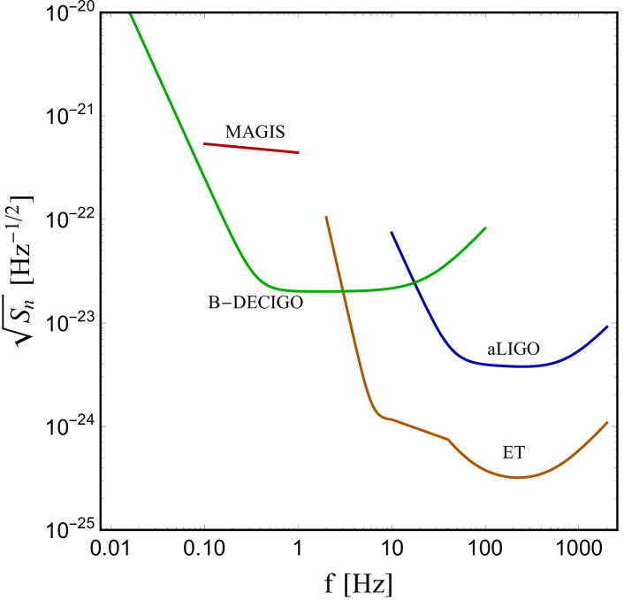
Figure 1: Square root of the noise power spectrum density of B-DECIGO, MAGIS, ET, and aLIGO.

We consider the GW detectors which are sensitive to the decihertz band $\mathcal{O}(0.1)$ Hz and the LIGO band $\mathcal{O}(100)$ Hz. The LIGO-band detectors are aLIGO at the design sensitivity LIGOScientific:2014pky and ET Punturo:2010zz . The decihertz detectors are the space-based B-DECIGO Kawamura:2018esd and MAGIS Graham:2017pmn . The square root of the noise power spectrum density $S_{n}(f)$ of the detectors are given in Fig. 1. To speed up numerical computation, we used the analytic fitting function $S_{n}(f)$ given in Ajith:2011ec , and Nakamura:2016hna . We used our own fitting functions for ET and MAGIS based on the curves plotted in Punturo:2010zz , and in Graham:2017pmn (Resonant mode), respectively.

We fix the frequency range of the LIGO-band detectors by $f_{\text{low}}=10\text{ Hz}$ and $f_{\text{high}}=(6^{3/2}\pi M)^{-1}$, i.e. the inner most stable circular orbit (ISCO) frequency. Although, in ET, we might extend the lower frequency limit to $2\text{ Hz}$, we choose $f_{\text{low}}=10\text{ Hz}$. By this way, the number of observed GW cycles in the aLIGO and ET are same, and therefore we can identify the difference coming from the shape of the $S_{n}(f)$. For the similar purpose, we give the common frequency range $f_{\text{low}}=0.1\text{ Hz}$ and $f_{\text{high}}=1\text{ Hz}$ to the decihertz detectors. In the frequency range $[0.1,1]\text{ Hz}$, since the inspiral lifetime $\tau$ Nishizawa:2016eza of the stellar mass binaries is at most $1.5$ year for $M=3\,M_{\odot}$ according to

$$\tau\simeq 1.5\text{ year}\left(\frac{f_{\text{low}}}{0.1\text{ Hz}}\right)^{-8/3}\left(\frac{M}{3\,M_{\odot}}\right)^{-5/3}\,,$$ (7)

it is safely within the mission lifetime of B-DECIGO and MAGIS which will be few years Kawamura:2018esd ; Graham:2017pmn .

IV Fisher matrix formalism

IV.1 Statistical errors

We estimate the statistical errors using the Fisher matrix. The Fisher matrix formalism relies on the assumption that the posterior probability distribution of GW parameters for a given data and model can be well approximated by the multivariate Gaussian distribution. Although the accuracy of the Fisher matrix calculation is limited to high Signal-to-noise ratio(SNR) cases Vallisneri:2007ev ; Rodriguez:2013mla , the Fisher matrix still can be used for the order of magnitude estimation of the parameter estimation.

The inverse of the covariance matrix $\Sigma^{ab}$ of the waveform model parameters can be approximated by the Fisher matrix $\Gamma_{ab}$ given by

$$\Sigma^{-1}_{ab}\simeq\Gamma_{ab}=\bigg{(}\frac{\partial h}{\partial\theta^{a}}\bigg{|}\frac{\partial h}{\partial\theta^{b}}\bigg{)}\,,$$ (8)

where $\partial h/\partial\theta^{a}$ denotes the partial derivative of the waveform model with respect to the model parameter $\theta^{a}$. With one-sided spectral density of the detector noise $S_{n}(f)$, $(h_{1}|h_{2})$ is defined by

$$(h_{1}|h_{2})\equiv 4\text{Re}\int_{f_{\text{low}}}^{f_{\text{high}}}df\frac{\tilde{h}_{1}^{*}(f)\tilde{h}_{2}(f)}{S_{n}(f)}\,,$$ (9)

where $f_{\text{low, high}}$ are the frequency range determined by the detector sensitivity and the binary total mass which will be described in the later section. The $\Gamma_{ab}$ is calculated in the parameter space

$$\theta^{a}=(\ln M,\eta,\chi_{1},\chi_{2},e_{0},t_{c},\phi_{c},\ln\overline{D})\,.$$ (10)

Note that, in this case, the whole Fisher matrix components become $\Gamma_{ab}\propto 1/\overline{D}^{2}$, where the scaling relation is also found in the SNR $\rho$ defined via

$$\rho^{2}\equiv(h|h)=4\int_{f_{\text{low}}}^{f_{\text{high}}}df\frac{|h(f)|^{2}}{S_{n}(f)}\propto\frac{1}{\overline{D}^{2}}\,.$$ (11)

Using the common scaling relation, we can normalize the $\Gamma_{ab}$ for a given SNR value. We consider the $\Gamma_{ab}$ with the $\rho=10$ or $\rho=100$ normalization. By this way, we can clearly see the influence of GW phase on the parameter estimation.

The Fisher matrix formalism has a weakness in dealing with the parameters with finite range. If the SNR is not high enough, the naively estimated statistical error of such parameters using the Fisher matrix can be unphysically large and show big discrepancies with the result using the full Bayesian analysis where the allowed range of parameters is naturally incorporated in the prior information Rodriguez:2013mla . One way to work around this limitation is to perturb the $\Gamma_{ab}$ by the Gaussian prior information $\Gamma_{aa}^{0}=(\delta\theta^{a})^{-2}$ (no summation in index $a$), where $\delta\theta^{a}$ is the width of the parameter range Favata:2013rwa ; Favata:2021vhw ; Cho:2022cdy . Therefore, we obtain the 1-sigma statistical errors by reading the diagonal components of the modified covariance matrix

$$\Sigma^{ab}\rightarrow\Sigma^{ab}=\left(\Gamma_{ab}+\Gamma^{0}_{ab}\right)^{-1}\,.$$ (12)

Since $\phi_{c}\in[-\pi,\pi]$, $\eta\in[0,0.25]$, $\chi_{1,2}\in[-1,1]$, and $e_{0}\in[0,1]$, we set

$$\delta\phi_{c}=\pi\,,\delta\eta=0.25\,,\delta\chi_{1,2}=1\,,\delta e_{0}=1\,.$$ (13)

IV.2 Systematic errors : FCV formalism

We estimate the systematic errors by the handy method developed by Culter and Vallisneri based on the Fisher matrix Cutler:2007mi (henceforth, FCV formalism). In the FCV formalism, the systematic bias $\Delta\theta^{a}$ between the true parameter $\theta_{T}^{a}$ of the true waveform $\tilde{h}_{T}=\mathcal{A}_{T}e^{i\Psi_{T}}$ and the best-fit parameter $\hat{\theta}^{a}$ given by a approximate waveform $\tilde{h}_{\text{ap}}=\mathcal{A}_{\text{ap}}e^{i\Psi_{\text{ap}}}$ is approximately given by

$$\begin{split}\Delta\theta^{a}&=\theta_{T}^{a}-\hat{\theta}^{a}\\ &\simeq\Sigma^{ab}\bigg{(}\frac{\partial h_{\text{ap}}}{\partial\theta^{b}}\bigg{|}[\Delta\mathcal{A}+i\mathcal{A}_{\text{ap}}\Delta\Psi]e^{i\Psi_{\text{ap}}}\bigg{)}\,,\end{split}$$ (14)

where $\Delta\mathcal{A}=\mathcal{A}_{T}-\mathcal{A}_{\text{ap}}$, $\Delta\Psi=\Psi_{T}-\Psi_{\text{ap}}$, and $\Sigma^{ab}$ is the covariance matrix given by Eq. (8). Here every quantities in the last line of Eq. (14) are calculated at $\theta^{a}=\hat{\theta}^{a}$.

We assume that the true amplitude and phase of the waveform are given by Eqs. (3b) and (5) as described in the Sec. II. Since the main goal of this work is estimating the systematic error $|\Delta\theta|$ of i) the quasi-circular waveform and ii) the $m$-PN accurate eccentric waveform, $\Delta\mathcal{A}=0$ and $\Delta\Psi$ is given by

$$\Delta\Psi=\frac{3}{128\eta v^{5}}\Delta\Psi^{\text{ecc}}_{\text{3PN}}$$ (15)

for the case i), and

$$\begin{split}\Delta\Psi&=\frac{3}{128\eta v^{5}}\left(\Delta\Psi^{\text{ecc}}_{\text{3PN}}-\Delta\Psi^{\text{ecc}}_{\text{mPN}}\right)\\ &=-\frac{7065}{187136}\frac{e_{0}^{2}}{\eta v^{5}}\left(\frac{v_{0}}{v}\right)^{19/3}\sum_{n=2m+1}^{6}c_{n}v^{n}\end{split}$$ (16)

for the case ii), where $c_{1}=0$. The PN order $m$ can be chosen between $0,1,1.5,2$ and $2.5$.

In our setting, Eq. (14) is reduced to

$$\Delta\theta^{a}\simeq 4\Sigma^{ab}\int_{f_{\text{low}}}^{f_{\text{high}}}df\frac{\mathcal{A}^{2}\partial_{b}\Psi_{\text{ap}}\Delta\Psi}{S_{n}(f)}\,.$$ (17)

Note that if we ignore the prior information $\Gamma_{ab}^{0}$, the scaling behavior of $\Sigma^{ab}\propto\overline{D}^{2}$ and $\mathcal{A}^{2}\propto\overline{D}^{-2}$ are opposite for a given $S_{n}(f)$, and therefore $\Delta\theta^{a}$ becomes SNR independent Cutler:2007mi . However, if we include $\Gamma_{ab}^{0}$ to $\Sigma^{ab}$ (Eq. (12)) (likewise in Favata:2013rwa ; Favata:2021vhw ; Cho:2022cdy ), the scaling relation does not hold anymore and $\Delta\theta^{a}$ becomes SNR dependent. The SNR independence is retrieved only when $\Gamma_{ab}\gg\Gamma_{ab}^{0}$. We will use the $\Sigma^{ab}$ given by Eq. (12) for Eq. (17) . Although using the $\Gamma_{ab}^{0}$ modified covariance matrix is somewhat lack of mathematical ground in the FCV formalism, the method is effective in the order-of-magnitude estimation of the systematic errors as shown by comparison with the full Bayesian analysis Favata:2021vhw ; Cho:2022cdy .

V Systematic errors due to ignoring eccentricity

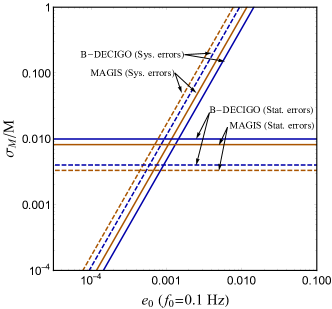
Figure 2: Fractional systematic and statistical errors of a binary total mass as a function of $e_{0}$ in B-DECIGO and MAGIS (left panel), and in aLIGO and ET (right panel). Binary total mass and symmetric mass ratio are set to $M=30\,M_{\odot}$ and $\eta=0.245$, respectively. Note that the reference frequency of each panel is $f_{0}=0.1\,\text{Hz}$ (left) and $f_{0}=10\,\text{Hz}$ (right), respectively. Solid (dashed) horizontal lines are statistical errors for $\rho=10$ ($\rho=100$). Up-ward sloping solid (dashed) lines are systematic errors for $\rho=10$ ($\rho=100$).

V.1 Scaling estimation

Before going into the results, we can make some simple scaling estimation for the statistical errors and the systematic errors that can be helpful for understanding the detector and parameter dependence of the results. If the correlation between parameters and the prior information are ignored, one can expect the statistical error $\sigma_{\theta}$ to be $\sigma_{\theta}\approx\Gamma_{\theta\theta}^{-1/2}\sim(\rho\partial_{\theta}\Psi)^{-1}$ Favata:2021vhw . It leads to the well-known lesson of the parameter estimation that the accuracy of the intrinsic parameters are proportional to the SNR and the number of GW cycles Cutler:1994ys .

To correctly estimate the errors of total mass $M$, the correlation between $M$ and $\eta$ should be taken into account. At the Newtonian order, $M$ and $\eta$ are totally degenerate, since the $\Psi$ only depends on the chirp mass $\mathcal{M}=M\eta^{3/5}$. The degeneracy is resolved by the 1 PN corrections to $\Psi$ which cannot be expressed in terms of the chirp mass only. Thus, using the number of GW cycle from the 1 PN correction $\Psi_{\text{1PN}}\propto 1/(\eta v^{3})$, the scaling estimation for $\sigma_{M}$ is

$$\sigma_{\ln M}=\frac{\sigma_{M}}{M}\sim\frac{1}{\rho\partial_{\ln M}\Psi_{\text{1PN}}}\sim\rho^{-1}\eta Mf_{\text{low}}\,,$$ (18)

where we ignore a weak dependence on $\eta$ given by the coefficient of 1 PN correction $a_{2}$. Here we used the fact that the most contributions to the integral Eq. (9) arise near $f=f_{\text{low}}$.

Scaling of the systematic error $\Delta\ln M=\Delta M/M$ can be estimated in a similar manner. From Eq. (17), one can obtain

$$\begin{split}\frac{\Delta M}{M}&\sim\left(\frac{\sigma_{M}}{M}\right)^{2}\rho^{2}\partial_{\ln M}\Psi\Delta\Psi\\ &\sim e_{0}^{2}(Mf_{\text{low}})^{-4/3}\,,\end{split}$$ (19)

where we used Eq. (15) and Eq. (18), and $e_{0}$ is defined at $f=f_{\text{low}}$. This crude estimation shows that the systematic error is SNR independent. Note that, however, if we include the prior information to calculate $\sigma_{M}/M$, which breaks down the scaling relation $\sigma_{M}/M\propto\rho^{-1}$, the systematic error can be also SNR dependent.

Since the systematic error is monotonically increasing function of $e_{0}$, we can define the critical eccentricity $e_{c}$, where

$$\Delta M(e_{c})=\sigma_{M}\,$$ (20)

is satisfied. From Eqs. (18) and (19), the expected scaling behavior of $e_{c}$ is

$$e_{c}\sim\rho^{-1/2}\eta^{1/2}(Mf_{\text{low}})^{7/6}\,.$$ (21)

V.2 Results

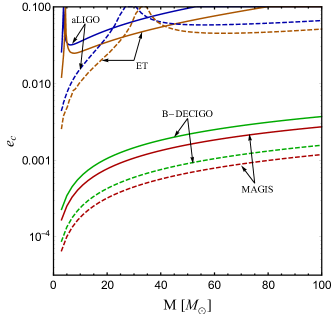
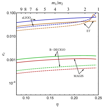
Figure 3: Critical eccentricity $e_{c}$ defined by Eq. (20) as a function of binary total mass (left panel), and symmetric mass ratio (right panel). Symmetric mass ratio $\eta$ is fixed to $0.245$ in the left panel, while binary total mass is fixed to $M=30\,M_{\odot}$ in the right panel. Solid (dashed) curves are $\rho=10$ ($\rho=100$) results for a given detector. Be aware of the definition of $e_{c}$ which is defined with $f_{0}=0.1\,\text{Hz}$ in B-DECIGO and MAGIS, and with $f_{0}=10\,\text{Hz}$ in aLIGO and ET.

Using the Fisher matrix formalism and the FCV formalism described in the Sec. IV.1 and IV.2, we estimate how small eccentricity can be problematic if we use the quasi-circular waveform for the parameter estimation of the eccentric binaries in the decihertz detectors, B-DECIGO and MAGIS. We also provide the estimation in aLIGO and ET, for a reference. Since the systematic errors of the source parameters due to ignoring the eccentricity increase as the eccentricity gets larger, the systematic errors can exceed the statistical error at some point Favata:2013rwa ; Favata:2021vhw . Finding such points can provide a useful guidance for the use of the quasi-circular or eccentric waveform.

In Fig. 2, we compare the statistical errors and systematic errors of $M$ within the initial eccentricity range $e_{0}<0.1$ for the decihertz detectors (left panel) and the LIGO-band detectors (right panel). Note that $e_{0}$ is defined at $0.1\text{ Hz}$ ($10\text{ Hz}$) for the decihertz (LIGO-band) detectors. The statistical errors are obtained from the quasi-circular waveform (Eq. (5) without $\Delta\Psi^{\text{ecc}}_{\text{3PN}}$). The phase difference which induces the systematic errors is given by Eq. (15). Here the intrinsic source parameters except $e_{0}$ are fixed to $M=30\,M_{\odot}$ (detector frame), $\eta=0.245$ and $\chi_{1,2}=0$. Each panel in Fig. 2 shows the results with moderate SNR $\rho=10$ (solid curves) and high SNR $\rho=100$ (dashed curves).

The left panel of Fig. 2 shows that the systematic errors given by the decihertz detectors with $\rho=10$ are monotonically increasing proportional to $e_{0}^{2}$ as expected by Eq. (19). When $e_{0}\gtrsim 0.001$, they eventually exceed the statistical errors. Similar trends also can be found in the LIGO-band detectors as shown in the right panel of Fig. 2 except that the critical eccentricity appears at $e_{0}\sim 0.05$ which is consistent with Favata:2021vhw . According to our scale estimations (as in Sec. V.1), the main factor that causes the $e_{c}$ difference between the decihertz and LIGO-band detectors is $f_{\text{low}}$. Smaller $f_{\text{low}}$ leads to the smaller statistical errors and the larger systematic errors. The effects are combined to give $\sim 50$ smaller $e_{c}$ in the decihertz detectors.

From Fig. 2, we see that the improvements in statistical errors are less than $10$ by comparing $\rho=10$ and $\rho=100$ cases. It is due to the prior information whose effects can be significant when the statistical error is comparable to the prior range. Since we use the prior-modified covariance matrix (Eq. (12)) for Eq. (17), the resulting systematic errors are also SNR dependent as shown in the figure. Comparing the decihertz and LIGO-band detectors, the SNR dependent systematic errors can be more clearly seen in the LIGO-band detectors due to the larger statistical errors.

Figure 3 shows $e_{c}$ as a function of $M$ (left panel) and as a function of $\eta$. In the left panel, we set $\eta=0.245$ and vary $M$ in the range $[3,100]\,M_{\odot}$. In the right panel, we set $M=30\,M_{\odot}$ and vary $\eta$ in the range $[0.08,0.245]$ which covers the mass ratio $m_{1}/m_{2}\sim 1.3$ to $m_{1}/m_{2}\sim 10$. The resulting curves are again divided in two classes, moderate SNR $\rho=10$ (solid curves) and high SNR $\rho=100$ (dashed curves). For brevity, we show $e_{c}$ from the different detectors in a single panel although the reference frequency of $e_{c}$ differs by detector.

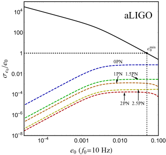
Figure 4: Fractional statistical errors of $e_{0}$ in B-DECIGO (left panel) and aLIGO (right panel) as a function of $e_{0}$. The statistical errors are shown in solid curves. Note that $e_{0}$ is defined at $f_{0}=0.1\,\text{Hz}$ for B-DECIGO, and at $f_{0}=10\,\text{Hz}$ for aLIGO. Binary total mass and symmetric mass ratio are set to $M=30\,M_{\odot}$ and $\eta=0.245$, respectively. Fractional systematic errors of $e_{0}$ due to using mPN-accurate eccentric phase are shown in dashed lines. We show the points at which $e_{0}^{\text{min}}$ and $e_{c}^{\text{mPN}}$ are defined. Here all results are obtained with $\rho=10$.

Figure 3 suggest that $e_{c}$ is typically $10^{-3}$ in the decihertz detectors with $\rho=10$. For $M=3\,M_{\odot}$ which corresponds to BNS-like binaries, $e_{c}$ can be as small as $10^{-4}$. $\rho=100$ cases result in much smaller $e_{c}$ values which can be as small as $\mathcal{O}(10^{-5})$. Although $e_{c}$ becomes larger for larger $M$ binaries, its value is still less than $\mathcal{O}(10^{-3})$. The higher mass ratio can slightly decrease $e_{c}$ but the change is small. The $e_{c}$ in MAGIS are smaller than that in B-DECIGO, because MAGIS is relatively more sensitive to $f_{\text{low}}=0.1\text{ Hz}$ thanks to its flat sensitivity curve. More specifically, when SNRs in the detectors are same, the SNR per frequency $d\rho/df$ of MAGIS is larger than that of B-DECIGO around $f_{\text{low}}=0.1\text{ Hz}$. All the behaviors of $e_{c}$ are consistent with the scaling estimation given by Eq. (21).

In Fig. 3, $e_{c}$ of the LIGO-band detectors are consistent with Favata:2013rwa ; Favata:2021vhw , where $e_{c}\sim\mathcal{O}(10^{-3}\sim 10^{-2})$. However, their strong SNR dependence is somewhat unexpected. We see that $e_{c}$ of $\rho=100$ is larger than $\rho=10$ for the binaries with $M\sim 30\,M_{\odot}$ and $\eta\sim 0.25$, which contradicts to the scale estimation. As already seen in Fig. 2, the non-trivial behavior is originated from the priors. Although the FCV formalism with priors is shown to be consistent with more accurate methods in the previous studies Favata:2021vhw ; Cho:2022cdy , this shows that the FCV formalism needs more validation in the prior-sensitive regime.

VI Range of measurable eccentricities

VI.1 Scaling estimation

Likewise in Sec. V.1, we make a crude scale estimations on the statistical error and the systematic error of the initial eccentricity $e_{0}$. Ignoring the correlations and the priors, from $\Gamma_{e_{0}e_{0}}\propto(\rho\partial_{e_{0}}\Psi)^{2}$, we have

$$\begin{split}\frac{\sigma_{e_{0}}}{e_{0}}&\sim\left(\rho\eta^{-1}v^{-5}\partial_{e_{0}}\Delta\Psi^{\text{ecc}}_{\text{3PN}}\right)^{-1}\\ &\sim\rho^{-1}e_{0}^{-2}\eta(Mf_{\text{low}})^{5/3}\,,\end{split}$$ (22)

where we approximate the integral by the value of the integrand at $f_{\text{low}}$. The eccentricity measurement is meaningful only when the $\sigma_{e_{0}}$ is smaller than the best-fit $e_{0}$. Note that the $\sigma_{e_{0}}$ is monotonically decreasing when $e_{0}$ is getting larger as shown by Eq. (22). Thus, we can define the minimum measurable eccentricity $e_{0}^{\text{min}}$ by

$$\sigma_{e_{0}}(e_{0}^{\text{min}})/e_{0}^{\text{min}}=1\,.$$ (23)

Using Eq. (22), its scaling is easily found to be

$$e_{0}^{\text{min}}\sim\rho^{-1/2}\eta^{1/2}(Mf_{\text{low}})^{5/6}\,.$$ (24)

In the following sections, we will focus on the systematic errors of $e_{0}$ due to ignoring eccentric PN corrections. Specifically, we test the accuracy of the mPN accurate eccentric waveform model with respect to the 3PN accurate waveform which is assumed to represent true signals. From Eqs. (16) and (17), the systematic errors of $e_{0}$ of the mPN eccentric waveform $\Delta e_{0}^{\text{mPN}}$ are

$$\begin{split}\frac{\Delta e_{0}^{\text{mPN}}}{e_{0}}&\sim\left(\frac{\sigma_{e_{0}}}{e_{0}}\right)^{2}\rho^{2}e_{0}\partial_{e_{0}}\Psi\Delta\Psi\\ &\sim\begin{cases}(Mf_{\text{low}})^{2/3}\,,&m=0\\[10.0pt] (Mf_{\text{low}})^{(2m+1)/3}\,,&m=1,\,1.5,\,2,\,2.5\end{cases}\end{split}$$ (25)

Note that $\Delta e_{0}^{\text{mPN}}/e_{0}$ are not determined by the number of GW cycles which scales as a negative power of $Mf_{\text{low}}$ but by the ignored mPN correction term which follows a positive power of $Mf_{\text{low}}$. It leads to smaller $\Delta e_{0}^{\text{mPN}}/e_{0}$ in the decihertz detectors. According to Eq. (22), $\sigma_{e_{0}}/e_{0}$ also gets smaller as $e_{0}$ increases, $\Delta e_{0}^{\text{mPN}}/e_{0}$ still can be larger than $\sigma_{e_{0}}/e_{0}$. Thus, we define $e_{c}^{\text{mPN}}$ by

$$\sigma_{e_{0}}(e_{c}^{\text{mPN}})=\Delta e_{0}^{\text{mPN}}\,,$$ (26)

where $\sigma_{e_{0}}$ is from the mPN accurate waveform model. The $e_{c}^{\text{mPN}}$ can be regarded as the maximum measurable eccentricity with the mPN waveform models. From Eqs. (22) and (25), the $e_{c}^{\text{mPN}}$ are expected to be

$$e_{c}^{\text{mPN}}\sim\begin{cases}\sqrt{\frac{\eta}{\rho}}\left(Mf_{\text{low}}\right)^{1/2}\,,&m=0\\[10.0pt] \sqrt{\frac{\eta}{\rho}}\left(Mf_{\text{low}}\right)^{\frac{2-m}{3}}\,,&m=1,\,1.5,\,2,\,2.5\end{cases}\,.$$ (27)

Smaller $e_{c}^{\text{mPN}}$ means more important systematic error. Therefore, Eq. (27) shows that the systematic error induced by the ignored PN corrections are likely to be more important in the decihertz detectors than in the LIGO-band detectors.

			$\rho=10$				$\rho=100$
Detector	$M\,[M_{\odot}]$	$\eta$	$e_{\text{min}}$	$e^{\text{0PN}}_{c}$	$e^{\text{1PN}}_{c}$	$e^{\text{1.5PN}}_{c}$	$e_{\text{min}}$	$e^{\text{0PN}}_{c}$	$e^{\text{1PN}}_{c}$	$e^{\text{1.5PN}}_{c}$
B-DECIGO	3	0.245	$2.2\times 10^{-4}$	$8.5\times 10^{-3}$	$7.3\times 10^{-2}$	-	$8.7\times 10^{-5}$	$3.5\times 10^{-3}$	$2.7\times 10^{-2}$	-
	30	0.245	$1.5\times 10^{-3}$	$2.7\times 10^{-2}$	-	-	$5.8\times 10^{-4}$	$1.1\times 10^{-2}$	$5.6\times 10^{-2}$	-
	100	0.245	$4.5\times 10^{-3}$	$5.5\times 10^{-2}$	-	-	$1.8\times 10^{-3}$	$2.2\times 10^{-2}$	$8.2\times 10^{-2}$	-
	30	0.08	$8.4\times 10^{-4}$	$1.5\times 10^{-2}$	$9.0\times 10^{-2}$	-	$3.7\times 10^{-4}$	$6.7\times 10^{-3}$	$3.3\times 10^{-2}$	-
MAGIS	3	0.245	$1.7\times 10^{-4}$	$6.7\times 10^{-3}$	$4.8\times 10^{-2}$	-	$4.4\times 10^{-5}$	$1.7\times 10^{-3}$	$1.6\times 10^{-2}$	$8.9\times 10^{-2}$
	30	0.245	$1.1\times 10^{-3}$	$2.1\times 10^{-2}$	-	-	$4.5\times 10^{-4}$	$8.4\times 10^{-3}$	$3.9\times 10^{-2}$	-
	100	0.245	$3.4\times 10^{-3}$	$4.2\times 10^{-2}$	-	-	$1.4\times 10^{-3}$	$1.7\times 10^{-2}$	$6.0\times 10^{-2}$	-
	30	0.08	$6.5\times 10^{-4}$	$1.2\times 10^{-2}$	$5.9\times 10^{-2}$	-	$2.9\times 10^{-4}$	$5.3\times 10^{-3}$	$2.4\times 10^{-2}$	-
aLIGO	3	0.245	$6.6\times 10^{-3}$	$5.3\times 10^{-2}$	-	-	$2.8\times 10^{-3}$	$2.3\times 10^{-2}$	-	-
	30	0.245	$5.0\times 10^{-2}$	-	-	-	$1.7\times 10^{-2}$	$6.5\times 10^{-2}$	-	-
	100	0.245	-	-	-	-	$5.4\times 10^{-2}$	-	-	-
	30	0.08	$2.8\times 10^{-2}$	-	-	-	$1.0\times 10^{-2}$	$4.0\times 10^{-2}$	-	-
ET	3	0.245	$4.7\times 10^{-3}$	$3.8\times 10^{-2}$	-	-	$2.9\times 10^{-3}$	$2.5\times 10^{-2}$	$4.0\times 10^{-2}$	-
	30	0.245	$3.5\times 10^{-2}$	-	-	-	$1.2\times 10^{-2}$	$4.6\times 10^{-2}$	-	-
	100	0.245	-	-	-	-	$4.2\times 10^{-2}$	-	-	-
	30	0.08	$2.0\times 10^{-2}$	$7.6\times 10^{-2}$	-	-	$7.5\times 10^{-3}$	$2.9\times 10^{-2}$	$9.5\times 10^{-2}$	-

Table 1: Minimum measurable eccentricities $e_{\text{min}}$ and maximum measurable eccentricities $e_{c}^{\text{mPN}}$ which are given by waveform models including the mPN-accurate eccentric phase. Various set of $M,\,\eta,\rho$, and detectors are considered. Results exceeding $0.1$ are left blank since the small eccentricity approximation becomes inaccurate for $e>0.1$. Note that $e_{\text{min}}$ and $e_{c}^{\text{mPN}}$ are defined at $f_{0}=0.1\,\text{Hz}$ for B-DECIGO and MAGIS, and at $f_{0}=10\,\text{Hz}$ for aLIGO and ET.

VI.2 Results

Using the methods described in Sec. IV.1 and IV.2, we estimate how small $e_{0}$ can be measured from the decihertz detectors. Furthermore, by examining the systematic error of $e_{0}$ from the eccentric PN corrections, we find how many eccentric PN corrections are required for $e_{0}$ measurement. Likewise in the previous sections, we consider B-DECIGO, MAGIS, aLIGO and ET. Again, note that $e_{0}$ is defined at $0.1\,\text{Hz}$ in the decihertz detectors and $10\,\text{Hz}$ in the LIGO-band detectors.

In Fig. 4, we show some examples of the statistical errors (black curves) and systematic errors (colored curves) of $e_{0}$ as a function of $e_{0}$. To show overall trend of the error estimations, we present the results only for B-DECIGO and aLIGO. Here we fix $M=30\,M_{\odot}$, $\eta=0.245$ and $\rho=10$. The statistical errors are obtained by the waveform model with $2.5$ PN accurate eccentric phase, although we find that changing the PN orders makes only negligible differences in the results. The mPN systematic errors are obtained by Eq. (17) with the phase difference between mPN eccentric waveform and 3PN eccentric waveform which are given by Eq. (16).

The left panel of Fig. 4 shows the results for B-DECIGO. We see that the statistical errors are clearly decreasing as $\sim e_{0}^{-2}$ as expected by Eq. (22) and the values can satisfy $\sigma_{e_{0}}/e_{0}<1$ for $e_{0}\gtrsim 10^{-3}$ which corresponds to detectable $e_{0}$ range. The $e_{0}$ dependence of the mPN systematic errors and the hierarchy between different PN orders are well explained by Eq. (25). We find that only the 0PN case can exceed the statistical error for large enough $e_{0}$. The other mPN cases might be able to exceed the statistical error for much larger $e_{0}$ but the results show that it happens only for $e_{0}>0.1$ where the small eccentricity assumption breaks down.

The right panel of Fig. 4 shows the results for aLIGO. The measurable eccentricity range is found to be $e_{0}\gtrsim 0.05$ which is consistent with Favata:2021vhw . It turns out that, for $e_{0}<0.1$, the systematic errors due to ignoring PN corrections are not significant.

The aLIGO cases in Fig. 4 have distinguished features compared to the B-DECIGO cases in two aspects. First, $e_{0}$ dependence of $\sigma_{e_{0}}/e_{0}$ and $\Delta e_{0}/e_{0}$ in the range $e_{0}\lesssim 0.001$ is not expected from Eq. (22). It can be understood by the prior $\Gamma_{e_{0}e_{0}}^{0}=1$. When $\Sigma^{e_{0}e_{0}}\sim(\Gamma_{e_{0}e_{0}}^{0})^{-1}=1$, it can be shown that $\sigma_{e_{0}}/e_{0}\propto e_{0}^{-1}$ and $\Delta e_{0}/e_{0}\propto e_{0}^{2}$. The relations can explain the results in $e_{0}\lesssim 0.001$. Seconds, the systematic errors of the 1.5 PN case larger than 1PN case and the similar discrepancy appears between the 2PN case and 2.5 PN case. This happens because, in the late inspiral, the contribution from $f_{\text{high}}$ cannot be ignored. At $f_{\text{high}}$, the hierarchy of the PN corrections can be inverted depending on the relative size of their coefficients.

Table 1 shows $e_{\text{min}}$ and $e_{c}^{\text{mPN}}$ for several $M$ and $\eta$ assuming $\rho=10$ or $\rho=100$. We choose detector frame total mass $M=3,\,30$, and $100\,M_{\odot}$ with $\eta=0.245$. To show $\eta$ dependence, $M=30\,M_{\odot}$ and $\eta=0.08$($m_{1}/m_{2}\sim 10$) is also considered. Since our methods rely on small eccentricity approximation, $e_{\text{min}},\,e_{c}^{\text{mPN}}>0.1$ cases are likely to be misleading. Those cases are left blank and, by the same reason, $e_{c}^{\text{2PN}}$ and $e_{c}^{\text{2.5PN}}$ cases in which every results are larger than 0.1 are not included in the table.

It turns out that B-DECIGO and MAGIS can measure $e_{0}$ as small as $\mathcal{O}(10^{-3})$ for stellar mass compact binaries with $\rho=10$. $e_{\text{min}}$ is improved (i.e. decreases) for smaller $M$ as expected from Eq. (24) and it can reach $10^{-4}$ level for $M=3\,M_{\odot}$ which is BNS-like system. For $\rho=100$, $e_{\text{min}}$ is improved by a factor $10^{1/2}$ and the typical values become $10^{-4}$ level. Larger mass ratio can also slightly improve $e_{\text{min}}$ as shown by $\eta=0.245$ and $\eta=0.08$ cases.

$e_{\text{min}}$ of aLIGO and ET in table 1 are $\mathcal{O}(10^{-2})$ for $M=\mathcal{O}(10)\,M_{\odot}$, which are $(10\text{ Hz}/0.1\text{ Hz})^{5/6}\sim 50$ larger than the decihertz detectors as expected by Eq. (24) . Unlike the decihertz detectors, aLIGO can ET can not measure $e_{0}$ of $M=100\,M_{\odot}$ very well for $e_{0}<0.1$, unless $\rho=100$. Overall, these results are consistent with the previous works Favata:2013rwa ; Favata:2021vhw .

$e_{c}^{\text{mPN}}$ set a upper bound on the measurable $e_{0}$ with the eccentric mPN waveform. In the decihertz detectors with $\rho=10$, the validity of 0PN eccentric phase is limited to $e_{0}\sim\mathcal{O}(10^{-2})$. However, even with 1PN eccentric phase, there is no limitation in $e_{0}$ measurement except for low total mass and high mass ratio cases. If $\rho=100$, 1PN eccentric phase can be problematic but increasing just 0.5PN order nearly solve the problem. In the LIGO-band detectors with $\rho=10$, even 0PN eccentric phase is accurate enough except for very low total mass or high mass ratio cases. 1PN eccentric phase is enough for aLIGO with $\rho=100$, while 1.5PN accuracy is required for ET with $\rho=100$. Overall, we find that 2PN (1.5PN) eccentric phase is accurate enough for low eccentricity measurement in the decihertz (LIGO-band) detectors.

VII Conclusions

In the various compact-binary formation scenarios Rodriguez:2018pss ; Antonini:2012ad ; Kowalska:2010qg , a non-negligible portion of the compact binaries are expected to have eccentricities $e_{0}\sim 10^{-4}$ at $f_{0}=0.1\,\text{Hz}$. In this paper we estimate the statistical errors of the GW intrinsic parameters and the systematic errors of them due to ignoring eccentricities. We adopt the Fisher matrix formalism Cutler:2007mi ; Favata:2013rwa for the error estimations. In B-DECIGO and MAGIS, we show that neglecting the eccentricities with $e_{0}\sim 10^{-4}-10^{-3}$ at $f_{0}=0.1\,\text{Hz}$ can induce the systematic errors exceeding the statistical errors. We find that the systematic errors become relatively more significant for smaller binary total mass, larger mass ratio, and larger SNR. We also estimate the ranges of measurable eccentricities with mPN accurate eccentric waveform models. An upper limit of the ranges is set by the systematic errors of eccentricities coming from the absent of the PN corrections. We show that B-DECIGO and MAGIS can measure eccentricity at least as small as $e_{0}\sim 10^{-4}-10^{-3}$ at $f_{0}=0.1\,\text{Hz}$. Therefore, detecting eccentric GWs is likely to be common in the decihertz detectors. We also find that, in the same detectors, omitting the high-order PN eccentric corrections does not significantly drop the accuracy of the eccentricity measurements. As a result, the eccentric waveform models with the 2PN eccentric corrections are enough for the measurement of eccentricities less than $0.1$ at $f_{0}=0.1\,\text{Hz}$.

In this work, we consider only the GW frequency with the twice of the orbital frequency. In principle, the multiple harmonics of the eccentric orbits can induce GW frequencies with integer times of the orbital frequency Yunes:2009yz . Although their amplitudes are so small in the small eccentricity limit, the decihertz detectors might be able to capture their signatures with their high sensitivity. To construct the efficient eccentric waveform models suited to the detectors, it is necessary to verify how many harmonics should be taken into account to avoid the systematic errors.

Quantifying the systematic errors in the moderate eccentricity regime ($0.1<e_{0}<1$) is also important issue that we did not cover(see, Moore:2019vjj for an aLIGO case). Since one cannot neglect higher harmonics as well as higher PN corrections in this case, there will be a lot of technical challenges. But considering the abundance of eccentric binaries at $0.1\text{Hz}$, our modeling accuracy on the GW sources should be clarified eventually.

Appendix : critical eccentricity with mass ratio and spins

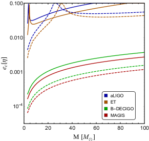
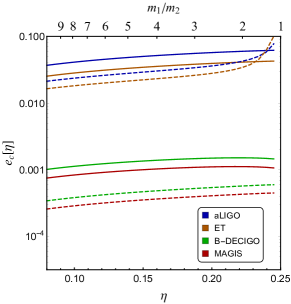
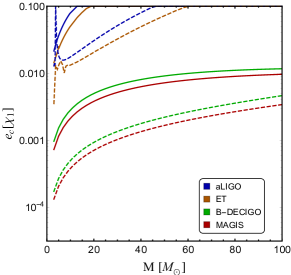
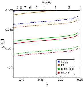
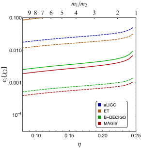
Figure 5: Critical eccentricity $e_{c}$ defined by $\eta$ ($e_{c}[\eta]$) and $\chi_{1,\,2}$ ($e_{c}[\chi_{1,\,2}]$) as a function of total mass $M$ (left panels) and $\eta$ (right panels) for the same systems assumed in Fig. 3. Solid curves (dashed) curves are $\rho=10$ ($\rho=100$) results. Note that $e_{c}$ are defined at $f_{0}=0.1\,\text{Hz}$ for B-DECIGO and MAGIS, and at $f_{0}=10\,\text{Hz}$ for aLIGO and ET.

In Sec. V, we studied the systematic errors due to ignoring the eccentricity parameter in terms of the critical eccentricity $e_{c}$. Since the systematic errors increase with $e_{0}$, we define $e_{c}$ as

$$\Delta\theta(e_{c})=\sigma_{\theta}\,,$$ (28)

where $\Delta\theta(e_{0})$ is the systematic error of a parameter $\theta$ as a function of $e_{0}$, and $\sigma_{\theta}$ is the statistical error of $\theta$. Note that smaller $e_{c}$ implies larger systematic errors. This appendix shows $e_{c}$ results with $\theta=\eta,\,\chi_{1}$, and $\chi_{2}$ which are not shown in the main text. They are denoted as $e_{c}[\theta]$. Figure 5 shows $e_{c}[\theta]$ as a function of binary total mass $M$ (left panels) and mass ratio $\eta$ (right panels) for the same systems assumed in Fig. 3. The $e_{c}[\eta]$ results are similar to the $e_{c}[M]$ results in Fig. 3, since both of them are mainly determined by the 1 PN correction to inspiral phase (see Eq. (18) and the above descriptions). The $e_{c}[\chi_{1,\,2}]$ are twice larger $e_{c}$ than $e_{c}[\eta]$. We find that it is due to large statistical error of $\chi_{1}$ and $\chi_{2}$. Overall, the $e_{c}$ results of the decihertz detectors are $10^{-4}-10^{-3}$, and therefore show that the parameter estimation with the detectors should take into account such small eccentricities.

References

- (1) B. P. Abbott et al. [LIGO Scientific and Virgo], Phys. Rev. X 9, no.3, 031040 (2019) doi:10.1103/PhysRevX.9.031040 [arXiv:1811.12907 [astro-ph.HE]].
- (2) R. Abbott et al. [LIGO Scientific and Virgo], Phys. Rev. X 11, 021053 (2021) doi:10.1103/PhysRevX.11.021053 [arXiv:2010.14527 [gr-qc]].
- (3) B. P. Abbott et al. [LIGO Scientific and Virgo], Astrophys. J. 883, no.2, 149 (2019) doi:10.3847/1538-4357/ab3c2d [arXiv:1907.09384 [astro-ph.HE]].
- (4) B. P. Abbott et al. [LIGO Scientific and Virgo], Astrophys. J. Lett. 882, no.2, L24 (2019) doi:10.3847/2041-8213/ab3800 [arXiv:1811.12940 [astro-ph.HE]].
- (5) R. Abbott et al. [LIGO Scientific and Virgo], Astrophys. J. Lett. 913, no.1, L7 (2021) doi:10.3847/2041-8213/abe949 [arXiv:2010.14533 [astro-ph.HE]].
- (6) B. P. Abbott et al. [LIGO Scientific and Virgo], Phys. Rev. Lett. 116, no.22, 221101 (2016) [erratum: Phys. Rev. Lett. 121, no.12, 129902 (2018)] doi:10.1103/PhysRevLett.116.221101 [arXiv:1602.03841 [gr-qc]].
- (7) B. P. Abbott et al. [LIGO Scientific and Virgo], Phys. Rev. Lett. 123, no.1, 011102 (2019) doi:10.1103/PhysRevLett.123.011102 [arXiv:1811.00364 [gr-qc]].
- (8) R. Abbott et al. [LIGO Scientific and Virgo], Phys. Rev. D 103, no.12, 122002 (2021) doi:10.1103/PhysRevD.103.122002 [arXiv:2010.14529 [gr-qc]].
- (9) J. Aasi et al. [LIGO Scientific], Class. Quant. Grav. 32, 074001 (2015) doi:10.1088/0264-9381/32/7/074001 [arXiv:1411.4547 [gr-qc]].
- (10) Y. B. Bae, C. Kim and H. M. Lee, Mon. Not. Roy. Astron. Soc. 440, no.3, 2714-2725 (2014) doi:10.1093/mnras/stu381 [arXiv:1308.1641 [astro-ph.HE]].
- (11) C. L. Rodriguez, S. Chatterjee and F. A. Rasio, Phys. Rev. D 93, no.8, 084029 (2016) doi:10.1103/PhysRevD.93.084029 [arXiv:1602.02444 [astro-ph.HE]].
- (12) D. Park, C. Kim, H. M. Lee, Y. B. Bae and K. Belczynski, Mon. Not. Roy. Astron. Soc. 469, no.4, 4665-4674 (2017) doi:10.1093/mnras/stx1015 [arXiv:1703.01568 [astro-ph.HE]].
- (13) J. Hong and H. M. Lee, Mon. Not. Roy. Astron. Soc. 448, no.1, 754-770 (2015) doi:10.1093/mnras/stv035 [arXiv:1501.02717 [astro-ph.GA]].
- (14) J. Samsing, M. MacLeod and E. Ramirez-Ruiz, Astrophys. J. 784, 71 (2014) doi:10.1088/0004-637X/784/1/71 [arXiv:1308.2964 [astro-ph.HE]].
- (15) J. Samsing, Phys. Rev. D 97, no.10, 103014 (2018) doi:10.1103/PhysRevD.97.103014 [arXiv:1711.07452 [astro-ph.HE]].
- (16) C. L. Rodriguez, P. Amaro-Seoane, S. Chatterjee, K. Kremer, F. A. Rasio, J. Samsing, C. S. Ye and M. Zevin, Phys. Rev. D 98, no.12, 123005 (2018) doi:10.1103/PhysRevD.98.123005 [arXiv:1811.04926 [astro-ph.HE]].
- (17) M. Zevin, I. M. Romero-Shaw, K. Kremer, E. Thrane and P. D. Lasky, Astrophys. J. Lett. 921, no.2, L43 (2021) doi:10.3847/2041-8213/ac32dc [arXiv:2106.09042 [astro-ph.HE]].
- (18) F. Antonini and H. B. Perets, Astrophys. J. 757, 27 (2012) doi:10.1088/0004-637X/757/1/27 [arXiv:1203.2938 [astro-ph.GA]].
- (19) J. Takátsy, B. Bécsy and P. Raffai, Mon. Not. Roy. Astron. Soc. 486, no.1, 570-581 (2019) doi:10.1093/mnras/stz820 [arXiv:1812.04012 [astro-ph.HE]].
- (20) H. Tagawa, B. Kocsis, Z. Haiman, I. Bartos, K. Omukai and J. Samsing, Astrophys. J. Lett. 907, no.1, L20 (2021) doi:10.3847/2041-8213/abd4d3 [arXiv:2010.10526 [astro-ph.HE]].
- (21) A. Nishizawa, E. Berti, A. Klein and A. Sesana, Phys. Rev. D 94, no.6, 064020 (2016) doi:10.1103/PhysRevD.94.064020 [arXiv:1605.01341 [gr-qc]].
- (22) A. Nishizawa, A. Sesana, E. Berti and A. Klein, Mon. Not. Roy. Astron. Soc. 465, no.4, 4375-4380 (2017) doi:10.1093/mnras/stw2993 [arXiv:1606.09295 [astro-ph.HE]].
- (23) K. Breivik, C. L. Rodriguez, S. L. Larson, V. Kalogera and F. A. Rasio, Astrophys. J. Lett. 830, no.1, L18 (2016) doi:10.3847/2041-8205/830/1/L18 [arXiv:1606.09558 [astro-ph.GA]].
- (24) B. Sun, Z. Cao, Y. Wang and H. C. Yeh, Phys. Rev. D 92, no.4, 044034 (2015) doi:10.1103/PhysRevD.92.044034
- (25) S. Ma, Z. Cao, C. Y. Lin, H. P. Pan and H. J. Yo, Phys. Rev. D 96, no.8, 084046 (2017) doi:10.1103/PhysRevD.96.084046 [arXiv:1710.02965 [gr-qc]].
- (26) H. P. Pan, C. Y. Lin, Z. Cao and H. J. Yo, Phys. Rev. D 100, no.12, 124003 (2019) doi:10.1103/PhysRevD.100.124003 [arXiv:1912.04455 [gr-qc]].
- (27) T. Yang, R. G. Cai, Z. Cao and H. M. Lee, [arXiv:2202.08608 [gr-qc]].
- (28) P. C. Peters and J. Mathews, Phys. Rev. 131, 435-439 (1963) doi:10.1103/PhysRev.131.435
- (29) P. C. Peters, Phys. Rev. 136, B1224-B1232 (1964) doi:10.1103/PhysRev.136.B1224
- (30) I. Kowalska, T. Bulik, K. Belczynski, M. Dominik and D. Gondek-Rosinska, Astron. Astrophys. 527, A70 (2011) doi:10.1051/0004-6361/201015777 [arXiv:1010.0511 [astro-ph.CO]].
- (31) S. Kawamura, T. Nakamura, M. Ando, N. Seto, T. Akutsu, I. Funaki, K. Ioka, N. Kanda, I. Kawano and M. Musha, et al. Int. J. Mod. Phys. D 28, no.12, 1845001 (2019) doi:10.1142/S0218271818450013
- (32) P. W. Graham et al. [MAGIS], [arXiv:1711.02225 [astro-ph.IM]].
- (33) R. Nair, S. Jhingan and T. Tanaka, PTEP 2016, no.5, 053E01 (2016) doi:10.1093/ptep/ptw043 [arXiv:1504.04108 [gr-qc]].
- (34) R. Nair and T. Tanaka, JCAP 08, 033 (2018) [erratum: JCAP 11, E01 (2018)] doi:10.1088/1475-7516/2018/08/033 [arXiv:1805.08070 [gr-qc]].
- (35) S. Isoyama, H. Nakano and T. Nakamura, PTEP 2018, no.7, 073E01 (2018) doi:10.1093/ptep/pty078 [arXiv:1802.06977 [gr-qc]].
- (36) M. A. Sedda, C. P. L. Berry, K. Jani, P. Amaro-Seoane, P. Auclair, J. Baird, T. Baker, E. Berti, K. Breivik and A. Burrows, et al. Class. Quant. Grav. 37, no.21, 215011 (2020) doi:10.1088/1361-6382/abb5c1 [arXiv:1908.11375 [gr-qc]].
- (37) P. W. Graham and S. Jung, Phys. Rev. D 97, no.2, 024052 (2018) doi:10.1103/PhysRevD.97.024052 [arXiv:1710.03269 [gr-qc]].
- (38) T. Yang, H. M. Lee, R. G. Cai, H. G. Choi and S. Jung, JCAP 01, no.01, 042 (2022) doi:10.1088/1475-7516/2022/01/042 [arXiv:2110.09967 [gr-qc]].
- (39) T. Nakamura, M. Ando, T. Kinugawa, H. Nakano, K. Eda, S. Sato, M. Musha, T. Akutsu, T. Tanaka and N. Seto, et al. PTEP 2016, no.9, 093E01 (2016) doi:10.1093/ptep/ptw127 [arXiv:1607.00897 [astro-ph.HE]].
- (40) K. Yagi and T. Tanaka, Prog. Theor. Phys. 123, 1069-1078 (2010) doi:10.1143/PTP.123.1069 [arXiv:0908.3283 [gr-qc]].
- (41) H. G. Choi and S. Jung, Phys. Rev. D 99, no.1, 015013 (2019) doi:10.1103/PhysRevD.99.015013 [arXiv:1810.01421 [hep-ph]].
- (42) M. Punturo, M. Abernathy, F. Acernese, B. Allen, N. Andersson, K. Arun, F. Barone, B. Barr, M. Barsuglia and M. Beker, et al. Class. Quant. Grav. 27, 194002 (2010) doi:10.1088/0264-9381/27/19/194002
- (43) C. Cutler and M. Vallisneri, Phys. Rev. D 76, 104018 (2007) doi:10.1103/PhysRevD.76.104018
- (44) M. Favata, Phys. Rev. Lett. 112, 101101 (2014) doi:10.1103/PhysRevLett.112.101101 [arXiv:1310.8288 [gr-qc]].
- (45) M. Favata, C. Kim, K. G. Arun, J. Kim and H. W. Lee, Phys. Rev. D 105, no.2, 023003 (2022) doi:10.1103/PhysRevD.105.023003 [arXiv:2108.05861 [gr-qc]].
- (46) H. S. Cho, Phys. Rev. D 105, 124022 (2022) doi:10.1103/PhysRevD.105.124022 [arXiv:2205.12531 [gr-qc]].
- (47) S. Tanay, M. Haney and A. Gopakumar, Phys. Rev. D 93, no.6, 064031 (2016) doi:10.1103/PhysRevD.93.064031 [arXiv:1602.03081 [gr-qc]].
- (48) S. Tanay, A. Klein, E. Berti and A. Nishizawa, Phys. Rev. D 100, no.6, 064006 (2019) doi:10.1103/PhysRevD.100.064006 [arXiv:1905.08811 [gr-qc]].
- (49) G. Cho, S. Tanay, A. Gopakumar and H. M. Lee, Phys. Rev. D 105, no.6, 064010 (2022) doi:10.1103/PhysRevD.105.064010 [arXiv:2110.09608 [gr-qc]].
- (50) A. Buonanno, B. Iyer, E. Ochsner, Y. Pan and B. S. Sathyaprakash, Phys. Rev. D 80, 084043 (2009) doi:10.1103/PhysRevD.80.084043 [arXiv:0907.0700 [gr-qc]].
- (51) C. K. Mishra, A. Kela, K. G. Arun and G. Faye, Phys. Rev. D 93, no.8, 084054 (2016) doi:10.1103/PhysRevD.93.084054
- (52) K. Chatziioannou, A. Klein, N. Yunes and N. Cornish, Phys. Rev. D 95, no.10, 104004 (2017) doi:10.1103/PhysRevD.95.104004 [arXiv:1703.03967 [gr-qc]].
- (53) B. Moore, M. Favata, K. G. Arun and C. K. Mishra, Phys. Rev. D 93, no.12, 124061 (2016) doi:10.1103/PhysRevD.93.124061
- (54) P. Ajith, Phys. Rev. D 84, 084037 (2011) doi:10.1103/PhysRevD.84.084037 [arXiv:1107.1267 [gr-qc]].
- (55) M. Vallisneri, Phys. Rev. D 77, 042001 (2008) doi:10.1103/PhysRevD.77.042001 [arXiv:gr-qc/0703086 [gr-qc]].
- (56) C. L. Rodriguez, B. Farr, W. M. Farr and I. Mandel, Phys. Rev. D 88, no.8, 084013 (2013) doi:10.1103/PhysRevD.88.084013 [arXiv:1308.1397 [astro-ph.IM]].
- (57) C. Cutler and E. E. Flanagan, Phys. Rev. D 49, 2658-2697 (1994) doi:10.1103/PhysRevD.49.2658 [arXiv:gr-qc/9402014 [gr-qc]].
- (58) N. Yunes, K. G. Arun, E. Berti and C. M. Will, Phys. Rev. D 80, no.8, 084001 (2009) [erratum: Phys. Rev. D 89, no.10, 109901 (2014)] doi:10.1103/PhysRevD.80.084001 [arXiv:0906.0313 [gr-qc]].
- (59) B. Moore and N. Yunes, Class. Quant. Grav. 37, no.22, 225015 (2020) doi:10.1088/1361-6382/ab7963 [arXiv:1910.01680 [gr-qc]].