PaST-NoC: A Packet-Switched Superconducting Temporal NoC

Abstract

Temporal computing promises to mitigate the stringent area constraints and clock distribution overheads of traditional superconducting digital computing. To design a scalable, area- and power-efficient superconducting network on chip (NoC), we propose packet-switched superconducting temporal NoC (PaST-NoC). PaST-NoC operates its control path in the temporal domain using race logic (RL), combined with bufferless deflection flow control to minimize area. Packets encode their destination using RL and carry a collection of data pulses that the receiver can interpret as pulse trains, RL, serialized binary, or other formats. We demonstrate how to scale up PaST-NoC to arbitrary topologies based on 2$\times$2 routers and 4$\times$4 butterflies as building blocks. As we show, if data pulses are interpreted using RL, PaST-NoC outperforms state-of-the-art superconducting binary NoCs in throughput per area by as much as $5\times$ for long packets.

I Introduction

Superconducting digital computing is a promising alternative to CMOS due to its ability to operate at several tens of GHz at a higher energy efficiency than CMOS [1, 2]. However, the full potential of superconducting digital computing is hindered by three major factors: First, the majority of superconducting digital rapid single flux quantum (RSFQ)  gates such as AND, OR, and XOR are synchronous, increasing the clock tree overhead and making scaling up challenging due to the need for precise timing [3, 4, 5]. Second, superconducting technology suffers from limited device density [6]. In fact, recent RSFQ chips were restricted to just a few tens of thousands of Josephson junctions, the fundamental switching device in superconducting computing. This limited density is exacerbated by the need of splitters which are interconnection cells that implement fanout, because of the severely limited inherent fanout of gates [3, 4, 5]. Third, superconducting memory is particularly area expensive [7]. These limitations, combined with adopting large, CMOS-inspired NoC control circuits and complicated wiring for wide buses to represent packets in binary, reduce area efficiency and restrict recent binary RSFQ NoCs to eight inputs and eight outputs at most [8, 9, 10, 11, 12, 13, 14].

In this work, we propose PaST-NoC that addresses current superconducting area density limitations by maximizing throughput per unit area. The key for the area efficiency of PaST-NoC is mapping control information such as packet destination as well as operating router control paths according to the time of arrival of RSFQ pulses using RL [5], instead of binary representation. In RL, information is mapped to the time of arrival of an RSFQ pulse (Figure 1).

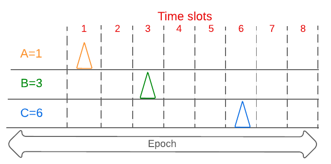
Figure 1: RL encodes values as time of arrival of pulses. Time is divided into repeating epochs that are divided into time slots, each denoting a value. A pulse arriving in time slot “I” represents the value “I”.

PaST-NoC is the first packet-switched NoC in RSFQ that operates its control path entirely in the temporal domain using RL and uses bufferless deflection flow control to avoid the elevated area cost of superconducting memory. As such, PaST-NoC provides tradeoffs that are more favorable to the unique characteristics of superconducting technology than traditional CMOS [15, 16]. The additional dynamic power due to deflections has a minimal impact in RSFQ [17, 1]. In addition, we propose a round-robin deflection policy [18] with randomization to provide probabilistic livelock freedom [19]. These novel contributions are described in Sections III and IV.

Although PaST-NoC’s control path operates entirely in RL for superior area efficiency, data can be encoded as serialized binary or unary, or a different encoding. Examples of unary encoding are RSFQ pulse streams, RL, or stochastic streams [20]. This makes PaST-NoC a candidate for conventional architectures that use typical binary encoding, but also for non-conventional architectures that use alternative data representations. These non-conventional architectures have demonstrated the potential for integrating hundreds of processing elements on today’s superconducting chips [20, 21, 22, 23, 24, 25, 26]. Not only do these scales motivate the use of a NoC but in fact previously-demonstrated binary superconducting NoCs are far from reaching the scales of hundreds that these emerging architectures call for. In addition, temporal PEs can readily generate control information such as packet destinations in the temporal domain that naturally fits PaST-NoC, instead of converting to binary in order to use binary NoCs.

PaST-NoC uses 2$\times$2 routers as a building block to reduce the area and complexity of its RL-based routing logic. Based on these 2$\times$2 routers, we describe how PaST-NoC easily scales up to a 4$\times$4 butterfly and an 8$\times$8 mesh that form the basis for a variety of larger topologies. To achieve this, we extend previous methods as described in Section V in order to effectively use them for PaST-NoC. When the data portion of packets is encoded using RL, PaST-NoC provides a higher throughput per port per area (calculated as number of JJs) compared to state-of-the-art binary RSFQ NoCs by over 5$\times$, and a statically-scheduled RSFQ temporal NoC [27] by as much as 2$\times$.

II Background and Motivation

TABLE I: A brief summary of superconducting logic primitives that appear in our study.

Name	Ins	Outs	Summary	Num of JJs
Splitter (S)	1	2	Produces a pulse at both outputs when receiving	3
			an input pulse. Implements fanout.
Merger (M)	2	1	Produces an output pulse when receiving	5
			a pulse at either input. Implements fanin.
Last arrival (LA)	2	1	Produces an output pulse as soon as it has	6
A re-purposed coincidence gate [5]			observed a pulse from each of its two inputs.
Inhibit (I)	2	1	Propagates a pulse from input 1 unless a	8
A re-purposed inverter cell [5]			pulse arrived at input 2 more recently than input 1.
Non-destructive read out (NDRO) cell [28]	3	1	Input pulses propagate to output if NDRO has observed a pulse in its	7
			SET control input more recently than a pulse in its reset control input.
Logical AND gate (AND)	3	1	Pulse at clock input causes output pulse if both	11
			data inputs received pulse since previous clock pulse.
Toggle flip flop (TFF) or (T)	1	2	First input pulse causes pulse at output 1,	10
			second at output 2, third at output 1, and so on.
Data flip flop (DFF)	2	1	Propagates input to output upon a readout (i.e.., clock) pulse.	4
Two-output data flip flop (DFF2)	3	2	DFF with one data input but two readout inputs, each with its own output.	12

II-A Superconducting Computing

II-A1 Fundamentals

Superconductivity is the property of certain metals to have zero resistance below a critical temperature that is usually a few Kelvins [1]. The fundamental superconducting switching device is the JJ [29]. The JJ allows current to pass through its two terminals with no resistance until a critical current $I_{c}$ is reached. Reaching $I_{c}$ causes the JJ to switch to a resistive state, causing a magnetic quantum flux transfer. This transfer is observable at the JJ terminal as a voltage pulse that lasts only a few picoseconds and has an amplitude of a few mVs [2]. Because JJs can switch in just a few picoseconds, they enable clock frequencies of several tens of GHz [8, 1, 5]. Moreover, superconducting digital computing promises energy-efficient computation even after accounting for cooling, due to the low JJ energy consumption which is several orders of magnitude lower than CMOS [1]. Cooling is already present in cryo-cooled systems such as quantum computers [24] and outer space electronics [30]. However, there is currently an approximate 1000$\times$ area density gap compared to CMOS [1, 6]. This limits superconducting digital circuits to small scales and memory sizes.

The most mature superconducting digital logic family is RSFQ and its variants [2]. In RSFQ, a logical 1 is encoded by the presence of a pulse and a logical 0 by the absence of a pulse. Because pulses (or their absence) are short-lived and travel at the speed of light, they are unlikely to arrive at logic gates at the same time. Therefore, RSFQ typically requires almost each gate in the design to be clocked, resulting in deeply-pipelined architectures; this increases the cost overhead associated with clock tree generation and distribution as well as makes timing closure challenging [3]. Importantly, fanout in RSFQ requires splitter cells that use three JJs each and have one input and two outputs. For instance, clocking 1024 synchronous gates requires 3072 JJs for 1024 splitters [31], a significant percentage of the overall design. RSFQ offers a rich set of traditional gates, such as ANDs, ORs, and data flip flops. Most gates are based on a superconducting loop that includes at least one JJ, called a superconducting quantum interference device (SQUID). SQUIDs preserve current where the intensity and direction of flow can be used to store state.

II-A2 Race Logic

RL in superconducting circuits is a form of temporal data representation and mitigates RSFQ’s low device density by trading area with time since a single wire can encode multiple values (Figure 1) [5]. In RL, a number is encoded as the time of arrival of a pulse within the computing time (epoch). For instance, if an epoch lasts 400ps and we define a “time slot” to be 50ps, there are eight time slots and thus a pulse can encode one of eight values. A pulse that arrives in the sixth time slot encodes the value 6, assuming the first time slot encodes the value 1. After the last time slot, a reset that is often called an epoch signal arrives and a new epoch begins.

RL computes by comparing the relative time of arrival of pulses. For instance, the last arrival (LA) gate produces an output pulse when the second of its two inputs observes a pulse. Because RL encodes data in the temporal domain, it is well-suited for dynamic programming [32]. Compute gates in RSFQ RL are stateful in order to remember what pulses arrived and their relative timing.

Table I summarizes the superconducting cells that appear in our study. We implement these cells based on designs from [5] and SUNY’s online library, except for the NDRO that is based on [28].

II-B NoCs and Deflection Flow Control

On-chip networks, also known as NoCs, typically consist of a set of routers that connect to each other and to endpoints in a manner defined by the topology [33]. NoCs have been commercially adopted [34, 35] and may use deterministic, oblivious, or adaptive routing. Moreover, the flow control defines how packets progress through the network. Because reducing area in CMOS is usually not the top priority, CMOS NoCs typically rely on input-queued buffered routers with credit-based backpressure to prevent buffer overflow. In contrast, using deflection flow control, a packet or flit never stalls or waits at routers [18, 15, 16]. Instead, if contention arises by having more than one packet requesting the same output, the router picks a winning packet to proceed. The losing packets are sent to any available outputs, which may lead the packets farther away from their final destinations. Bufferless flow control is attractive for an RSFQ NoC due to the stringent area constraints and the elevated cost of superconducting memory [7]. By using deflection flow control, we eliminate router buffers at the expense of a marginal increment in dynamic power. This increment in dynamic power has a negligible impact due to RSFQ’s dynamic energy efficiency [17, 1].

II-C Related Work

In RSFQ, demonstrated NoCs have focused on a binary representation and have been limited to no more than eight inputs and outputs because they mostly use CMOS-inspired control such as for routing and allocation, as well as multiple parallel wires to represent packets in binary. As a result, these NoCs are not adequately area-efficient to scale up further given RSFQ’s device density [8, 9, 10, 11, 12, 13, 14]. In particular, previous work demonstrated 2$\times$2 [10, 11] and $4\times$4 [8, 9] crossbar switches including schedulers [14], a 3$\times$3 ring [13], and larger mesh or Banyan networks (that are topologically equivalent to a butterfly network) [12].

Further past work on NoCs used temporal encoding only in the data path (not in the control path) by temporally encoding packet payloads in CMOS [36] and in RSFQ [27]. In particular, superconducting rotary NoC (SRNoC) [27] follows a rigid rotating schedule. Thus, its performance suffers under unbalanced traffic patterns. Also, depending on the number of routers, SRNoC may require potentially deep buffers at network boundaries for packets to wait for their desired connection to be established. Our proposed PaST-NoC is the first packet-switched NoC that operates its control in the temporal domain using RL and offers a versatile data path.

III Packet format

This and the next two sections describe the novel contributions of this paper. Consistent with our design goal to operate PaST-NoC’s control path entirely temporally, PaST-NoC uses a packet format that is encoded in the temporal domain using RL. Following the RL convention, a packet’s duration is equal to an epoch, which is defined by a periodic signal. The epoch signal serves to reset the values that RL pulses represent and also helps re-synchronization at pre-defined NoC boundaries, as we discuss later. The epoch duration is constant throughout the NoC.

Packets traverse the NoC as a unit and cannot be divided or merged with other packets. As shown in Figure 2, packets have control information that is succeeded by data. Control information is encoded using RL. Control and data boundaries are defined by a duration that is a subset of an epoch that we name a “period”. For example, if the epoch lasts 500ps, the control period can last 200ps and the data 300ps.

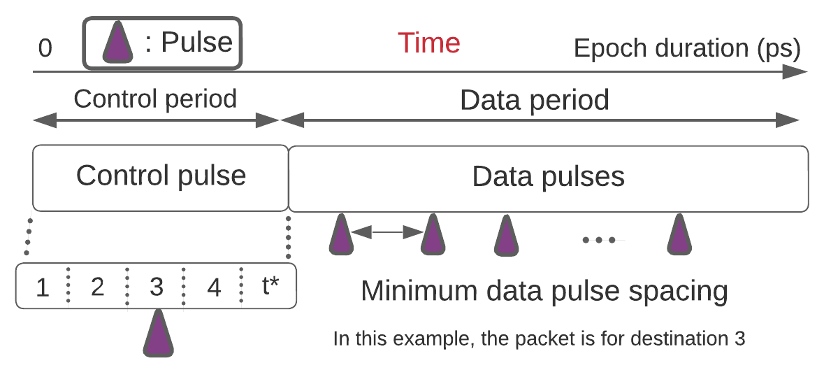
Figure 2: PaST-NoC’s packet format. The control period has exactly one pulse encoded in RL to signify the packet’s final destination. In this example, there are four potential destinations. The last control time slot (labelled $t*$) does not contain a pulse but gives the routing logic sufficient time to produce results. Time elapses from left to right.

III-A Data Period

The data period contains pulses that are interpreted only by the receiver, not routers. Therefore, data pulses can be encoded in RL or any other format the receiver expects. For example, if terminals are neurons in RSFQ and PaST-NoC implements the connection in a neuromorphic processor [25], packets can carry pulse trains. Alternatively, packets can carry binary values that are transported serially.

Without loss of generality, in our work, we assume data pulses are encoded in RL similar to control pulses. To that end, data periods are divided into “time slots” where each slot denotes a value. For instance, a pulse in the third slot encodes the value of 3, assuming that the first slot encodes the value of 1 ($B$ in Figure 1). To compare against binary, the length of a data period determines the equivalent bit resolution that each data pulse represents. For $b$ bits of resolution, we need $2^{b}$ time slots. For example, with a bit resolution of 3, we can represent 8 different numbers (e.g., 0-7) and thus the packet’s data period has eight time slots. The duration of the data period and the number of data pulses in each data period are application-dependent.

With this encoding, a packet can carry as many RL pulses as time slots, as long as each time slot has at most one RL pulse. In case of conflicts, that is when we need to send two pulses with the same RL value, we can distribute these conflicting data pulses in different packets. Therefore, the number of data pulses per packet (the amount of data a packet carries) depends on the data’s value. We do not tailor our evaluation to a particular application. Thus, we evaluate a range of data period durations and assume that data pulses can fall at any time slot in the data period with a uniform random probability. This way, if we assume that $n$ is the number of available time slots in the packet’s data period and we also try to fit $n$ data pulses per packet, we can use the bins and balls model [27] to calculate the approximate number of data pulses $m$ we can fit per packet without conflicts (at most one pulse per time slot) as:

$$m=n-\frac{n}{e}$$ (1)

where $e$ is the exponential constant or Euler’s number. For example, for $b=5$ and $n=2^{b}=64$, the expected number of data pulses per packet is $m=40.1$.

III-B Control Period

The control period contains a single pulse that follows the RL convention and encodes the packet’s final destination. In the example of Figure 2, the packet is destined to destination number three out of four possible destinations. As PaST-NoC scales up, the control period is prolonged to contain a time slot for each potential destination. In addition, we add a time slot at the end of the control period where we do not expect a pulse. This slot provides the routing logic sufficient time to produce a result before the end of the control period and thus configure the router’s data path without violating cell setup times due to data pulses arriving prematurely. Thus, a control period for a four-destination PaST-NoC has five time slots.

IV Router architecture

PaST-NoC implements bufferless deflection flow control [18, 15, 16] to avoid the area cost of memory because RSFQ’s restricted device density makes area a primary constraint. Moreover, the additional dynamic energy for deflections has a relatively small impact in RSFQ. To keep design complexity low, PaST-NoC routers have two inputs and two outputs (2$\times$2). Therefore, if two incoming packets request the same output (a conflict), one proceeds to its requested output and the other is deflected to the other output that is guaranteed to be available since there is an equal number of inputs and outputs.

IV-A Router Overview

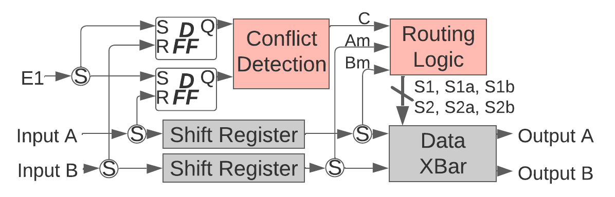
Figure 3: A PaST-NoC 2$\times$2 router. Data path components are in gray (bottom) and control path components in red (top). “S” circles are splitter cells.

Figure 3 shows a block-level diagram of a PaST-NoC 2$\times$2 router. The splitter and DFF at each input (A and B) send only the first pulse that arrives at each input, i.e., the pulse at each packet’s control period, to the conflict detection logic. In parallel, the entirety of the packet from each input traverses a shift register. The shift register along that path delays the packet by a period of time equal to one control period duration. This allows the conflict detection logic to produce its output $C$, which is propagated to the routing logic (Section IV-B).

The shift register has a number of stages equal to the control period divided by the minimum spacing between data pulses, since we find that it is smaller than the minimum spacing between control pulses and data pulses also traverse the shift register. Each stage has a duration equal to the minimum spacing between data pulses. This duration also defines the period of the local clock signal that each shift register requires. For instance, for a control period duration of 150ps and a data pulse spacing of 15ps, each shift register has $\frac{150}{15}=10$ stages of 15ps each. To reduce the JJ count as delay scales, we base our implementation on a flux-based shift register [37].

The first pulse that exits the shift register in an epoch, which is the control pulse of each packet, is propagated to the routing logic. After receiving $C$ from the conflict detection logic, the routing logic produces its outputs. We label the delayed (post shift register) version of $A$ as $A_{m}$ and likewise $B_{m}$ for $B$. The routing logic also receives data pulses after the control pulse through $A_{m}$ and $B_{m}$, but data pulses have no effect in this block.

PaST-NoC routers receive a threshold input ($Thr$) to help map packet destinations to router outputs; if a packet’s control pulse arrives before $Thr$, it requests the first (top) router output, otherwise the second (bottom) output. As we later explain, the time interval between epoch start ($E1$) and $Thr$ that a router receives depends on the router’s position in the NoC.

The primary outputs of the routing logic are $S1$ and $S2$. $S1$ causes the data crossbar to connect input $A$ to output $A$ and input $B$ to output $B$; $S2$ causes the opposite. A pulse in $S1$ is asserted when there is no conflict and at least one packet from input $A$ requested output $A$ or a packet from input $B$ requested output $B$. Likewise, a pulse in $S2$ is asserted when at least one packet from input $A$ requested output $B$ or a packet from input $B$ requested output $A$. In the case of conflict, the routing logic can resolve it with a pulse at $S1$ or $S2$ because either will route one of the two packets to its desired output. Finally, if there is only one incoming packet, control signals $S1$ or $S2$ connect the input that does not receive a packet with an available output, but this has no adverse effect since no pulses traverse that path.

IV-B Routing logic

The router’s control logic is based on RL and is responsible for decoding the desired destination of each packet, resolving conflicts, and configuring the data crossbar before data pulses traverse the crossbar. This logic can be designed to follow a fixed-priority or a round-robin scheme. We use fixed priority as a building block for round robin.

IV-B1 Fixed Priority Routing logic

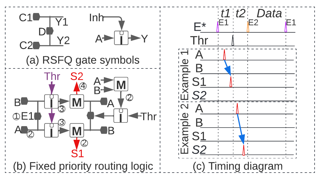
Figure 4: (a) Here we show the diagrams of two separate gates that appear later. On the left, we show a DFF2 that has two readout (or clock) inputs ($C1$ and $C2$), one data input ($D$), and two data outputs ($Y1$ and $Y2$). A pulse at input $C1$($C2$) generates a pulse at output $Y1$($Y2$) if there was a prior pulse at input $D$. On the right is an inhibit cell that has a data input ($A$), data output ($Y$), and an inhibit control input ($Inh$). An incoming pulse to input $A$ is propagated to output $Y$ unless a pulse arrived at $Inh$ more recently than the pulse at $A$. (b) Circuit for the fixed priority routing logic. (c) An example of one packet arriving in $A$, before and after the threshold ($Thr$). $E*$ is not a separate signal but rather a notation to illustrate the arrival of both $E1$ and $E2$ in the same waveform line.

The fixed priority routing logic always resolves a conflict in favor of the packet whose control pulse arrives first. This can result in unfair bandwidth allocation, especially under heavy load. On the other hand, this compact routing logic uses a low number of JJs. The fixed priority routing logic can be built using two two-output data flip flops connected facing each other as shown in Figure 4(b). The DFF2 on the left is set by pulse $E1$ that marks the beginning of the epoch ①. The DFF2 on the left then waits for $A$ and $B$ to arrive before $Thr$. If $A$ ($B$) arrives first, $S1$ ($S2$) is produced and the DFF2 on the right is never enabled (i.e., its data input never receives a pulse) because of the inhibit cell ②. In the case that neither $A$ nor $B$ arrive before the threshold ($Thr$), the DFF2 path on the left side is disabled by $Thr$ through the inhibit cells ③ and the DFF2 on the right is enabled by $Thr$. In this case, if $A$ ($B$) arrives first, $S2$ ($S1$) is set ④. Figure 4(c) shows two examples where $S1$ and $S2$ are generated.

IV-B2 Conflict Detection

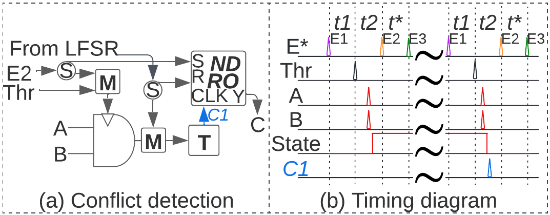
Figure 5: (a) A circuit diagram of the conflict detection logic. $T$ is a TFF, $S$ is a splitter cell, and $M$ is a merger cell. (b) A timing diagram that illustrates its operation. $t*$ is the extra control period time slot. $E1$ denotes the beginning of the epoch and thus also the packet’s control period, $E2$ the beginning of $t*$, and $E3$ the end of the control period. $E*$ is not a separate signal but rather a notation to illustrate the arrival of both $E1$ and $E2$ in the same waveform line.

To aid the round-robin routing logic that follows, we design a conflict detection logic to detect when packets from both inputs request the same output. This happens when the control pulse from inputs $A$ and $B$ arrive both before or both after $Thr$. In case of conflict, this unit changes its internal state and generates a pulse ($C1$) every second conflict. This results in a round-robin resolution of conflicts.

Figure 5 illustrates the conflict detection circuit and an example of operation. The AND gate generates an output pulse if both control pulses arrive between $E1$ and $Thr$ or between $Thr$ and $E2$. If the condition is met, the TFF changes its state. $E1$ marks the beginning of an epoch, $E2$ the end of the second time slot in the control period (the beginning of $t*$), and $E3$ the beginning of the data period. In Figure 5(b), $A$ and $B$ conflict because they request the same output. That does not produce a $C1$ output pulse, but it changes the TFF’s internal state. At the next epoch with a conflict, the circuit produces a $C$ pulse and reverts the TFF’s internal state. Note that $E2$, $E3$, and $Thr$ pulses are periodic control signals. Therefore, the conflict detection logic is in principle synchronous because it uses these control signals for timing and to clear its state between epochs. These signals can be either globally distributed or locally derived inside the router from $E1$ using constant delays such as with Josephson transmission lines.

IV-B3 Round-Robin Routing Logic

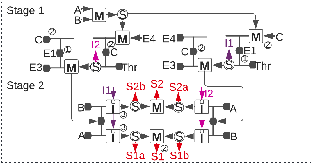
Figure 6: The two-stage round-robin routing logic.

This logic promotes fairness. When two incoming packets request the same output (a conflict), the routing logic picks a winner packet in a round-robin fashion and deflects the loser packet to the other (not requested) output. Figure 6 shows the round-robin routing logic, which is divided into two stages. The first stage uses the conflict signal ($C$) as input and prepares the second stage. The second stage operates similarly to the fixed-priority logic described above.

The first stage’s primary task is to flip $E1$ and $Thr$ between left and right when it receives a pulse in $C$. This stage is composed of two pairs of DFF2s facing each other (left and right) through mergers. This stage initially assumes there is no conflict and sets the outer sides of the pairs ① with $E1$. When $E3$ arrives, it propagates through the left DFF2 at the left pair of the first stage setting the left side of the second stage, which behaves as the fixed priority routing logic of Section IV-B1. In case of conflict, the outer sides of the first stage pairs are reset by $C$ while the inner sides of the pairs are set ②. Also, $E3$ sets the right side of the second stage and $Thr$ sets its left side, achieving a complementary effect. To reduce area, we remove JJs for unused DFF2 outputs (two JJs per unused output).

The second stage is built and behaves similarly to the fixed priority routing logic, except that its inputs are $A_{m}$ and $B_{m}$. Also, the second stage’s two sides are symmetric given that $E3$ and $Thr$ can arrive at both sides, depending on the first stage. Furthermore, because control pulses are used by the routing logic to configure the data crossbar, control pulses arrive at the crossbar through the data path before the routing logic has a chance to generate $S1$ or $S2$ to configure the crossbar. This would cause control pulses to be dropped. Therefore, we use splitters in the second stage of the routing logic to generate intermediate signals $S1_{a}$, $S1_{b}$, $S2_{a}$, and $S2_{b}$; we use these signals to re-generate packet control pulses. Essentially, these four signals codify which input–output combination was selected and which inputs received a packet. For instance, $S1_{a}$ ($S2_{a}$) is asserted when a packet arrived at input $A$ and has been assigned output $A$ ($B$). The new control pulse as a result of these four signals will still be in the same control time slot as the original, thus preserving the packet’s encoded destination.

Using $A_{m}$ and $B_{m}$ provides the necessary time for the conflict-detection circuit to identify a conflict and achieve the round-robin deflection algorithm. However, this causes the entire packet to be delayed by a control period, giving the illusion to the control path of two control periods. This is illustrated in Figure 7. The first period uses $A$ and $B$ and activates the conflict detection logic while the second uses $A_{m}$ and $B_{m}$ and activates the routing logic. The epoch begins when $E1$ arrives and starts the first time slot ($t1$). The second time slot in the first control period ($t2$) starts when $Thr$ first arrives and ends when $E2$ arrives. Between $E2$ and $E3$ is the extra time slot ($t*$). The second control period is from $E3$ until $E4$. In this example, $A$ and $B$ arrive after $Thr$, indicating that both packets request the same (second) output. Assuming this is the second time this occurs, a conflict pulse ($C$) is generated during the first control period’s extra time slot ($t*$). In the shown example, the routing logic resolves this conflict with a $S2$.

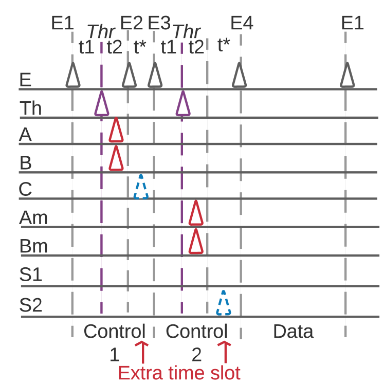
Figure 7: From the control path’s perspective, there are two control periods.

IV-B4 Randomized Round-Robin Routing Logic

While the round-robin routing logic makes each router divide bandwidth evenly across its inputs by average, under specific circumstances it may cause a packet to be deflected in perpetuity, thus leading to a livelock [16]. For instance, consider the case where a packet that arrives to a router’s input 1 gets deflected because the round robin for the packet’s desired output favors input 2; input 2 receives another packet for the same output in the same epoch. Further, lets assume that the deflected packet arrives at an adjacent router at the next epoch and then returns to the router it was deflected at, because that is the shortest path to its final destination. This can occur in the PaST-NoC 2D mesh that we describe later. Therefore, the deflected packet arrives to the same router two epochs after it was initially deflected since it has to take two hops. Two epochs after it was deflected, the round robin for the packet’s desired output again favors input 2, whereas in this example the packet again arrives to input 1. This process may repeat in perpetuity if input 2 always receives packets that request the same output that conflict with the deflected packet, and the deflected packet returns and re-tries after an even number of epochs. While maintaining these conditions in perpetuity with dynamic traffic is improbable, it is possible.

To prevent livelocks in PaST-NoC, we take a probabilistic approach inspired by the “chaos” router [19]. The intuition behind this approach is that we add randomness in routing decisions such that the repetitious routing patterns that form a livelock eventually decay. Therefore, any packet has a nonzero probability at every hop of not getting deflected, which means that every packet will eventually get delivered. This results in a probabilistically livelock-free NoC [19]. To that end, we add randomness to the round-robin conflict detection unit.

Our proposed conflict detection unit has two modes of operation: pure round robin and randomized round robin. To set one mode of operation or the other we use an non destructive read out (NDRO) cell at the output of the conflict detection logic (Figure 5a). If an RSFQ pulse produced randomly by a pseudo random number generator (PRNG) such as an linear-feedback shift register (LFSR) does not arrive, the NDRO is transparent because it is set by $E2$ before the conflict detection logic produces a conflict pulse $C1$. Therefore, the router behaves in a pure round-robin fashion. In contrast, in the presence of a random pulse, the NDRO is reset. This suppresses the propagation of the conflict pulse $C1$, thus breaking the round-robin sequence. In this case, even if the logic detects a conflict, the routing logic behaves like the fixed-priority routing logic instead of round robin. Finally, the pulse from the PRNG is also routed to the TFF in order to disrupt the round-robin counter. The insight behind this modification is to allow the conflict detection logic to operate in a round-robin fashion some times, but randomly break the round robin thus disrupting the conditions that cause a livelock other times [19].

To implement a PRNG, we can use existing RSFQ multi-bit PRNGs such as LFSRs [38, 39] or other custom PRNGs [40]. We can use a single PRNG for the entire NoC by connecting each bit of a multi-bit PRNG to a different PaST-NoC router.

While in CMOS a popular solution to livelocks is a form of age-based allocation [41, 16, 15], this would substantially increase routing logic complexity, the number of JJs, and the complexity of a packet’s control period. Instead, our proposed solution only adds three cells per router and a PRNG per NoC. In addition, it does not prolong control periods or other parameters that would degrade throughput or latency.

However small, the area overhead for randomization is not justified for traffic patterns that cannot produce a livelock due to their source–destination pairs or because they pause injecting packets periodically, allowing deflected packets to be delivered. Therefore, in our evaluations in Section VI, we use the round-robin routing logic of Section IV-B3 without randomization. However, if livelock prevention is desired, the additional overhead is 24 JJs per router and additional JJs for the PRNG depending on its implementation [38, 39, 40].

IV-C Data path

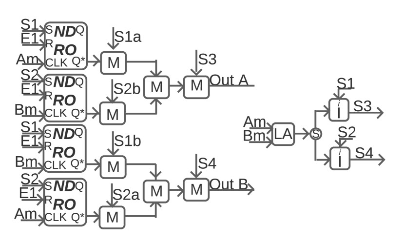
Figure 8: The data crossbar relies on NDRO cells to connect each input–output pair. A pulse in $S1$ connects input $A$ to output $A$ and input $B$ to output $B$. A pulse in $S2$ connects input $A$ to output $B$ and input $B$ to output $A$. In parallel, the data crossbar also generates $S3$ and $S4$.

Figure 8 shows PaST-NoC’s data crossbar that consists of NDROs and mergers. $S1$ sets the first and third NDROs from the top, connecting input $A$ to output $A$ and input $B$ to output $B$. $S2$ sets the other two NDROs, achieving a complementary effect by connecting input $B$ to output $A$ and input $A$ to output $B$. $A_{m}$ and $B_{m}$ connect to the clock input of the NDROs. A pulse in the clock input of an NDRO causes an output pulse if the NDRO has received a pulse in its set ($S$) input more recently than a pulse in its reset ($R$) input (i.e., the NDRO is “set”). Therefore, incoming packet pulses through $A_{m}$ and $B_{m}$ are propagated by NDROs that are set. Finally, $E1$ resets all NDROs to clear the state of all NDROs between epochs.

In parallel, the crossbar also generates $S3$ and $S4$ that supplement $S1_{a}$, $S1_{b}$, $S2_{a}$, and $S2_{b}$ by reconstructing control pulses in the cases where there are two incoming packets. For this, we design a resettable LA gate shown in Figure 9.

Figure 9: A resettable LA gate composed of two DFF2s and one merger.

V Scaling Up

We can scale up PaST-NoC based on the proposed 2$\times$2 router. We first design a 4$\times$4 butterfly NoC that we then use as a building block for an 8$\times$8 mesh. These building blocks can then construct a PaST-NoC of various scales and topologies.

V-A 4$\times$4 Butterfly

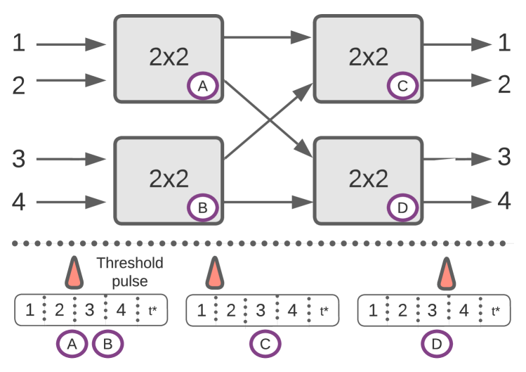
Figure 10: A 4$\times$4 butterfly composed of four 2$\times$2 routers. Depending on its position (Ⓐ, Ⓑ, Ⓒ, or Ⓓ) each router has a different timing for its threshold pulse ($Thr$) according to how destinations are mapped to its outputs.

A 4$\times$4 butterfly is shown in Figure 10. Each path consists of two hops and there is exactly one path from each source to each destination, which means routing is deterministic. A butterfly is topologically equivalent to a Banyan topology [12, 11]. We design a 4$\times$4 NoC with a butterfly instead of scaling up a single router to keep router design complexity low.

To correct for the propagation delay of pulses through the first column routers, $E1$, $E2$, $E3$, and $Thr$ in the routers of the second column are delayed by the propagation delay through a router. For example, if the propagation delay (latency) of a router is $PD$, all periodic control pulses to routers in the second column are delayed by $PD$. Otherwise, packets would exit a router in the first column and arrive late at a second-column router, risking that their control and data pulses would appear to be in different time slots. Likewise, final destinations also delay their epoch start by the propagation delay through two routers ($2\times PD$), which is the end-to-end propagation delay of this network. The packet latency is $2\times PD+EpochDuration$ because it includes the time from when a packet starts arriving until it completes. Note that this discussion applies to any $N$ hop path (in this case $N$ = 2). An alternative strategy is to prolong time slots to account for propagation delays [27], though that risks degrading throughput.

In this topology, if a packet gets deflected at a router in the first or second column, it will exit the NoC at a destination it did not intend. Destinations are responsible for re-injecting any packets they receive that are not destined to them [16].

Figure 10 also shows how the timing of the threshold pulse ($Thr$) changes per router, depending on the router’s location. This is necessary because each 2 $\times$ 2 router sends to its top output any packet with a control pulse before $Thr$ and others to its bottom output. Therefore, adjusting the timing of $Thr$ at each router is necessary to correctly route packets to final destinations. From routers Ⓐ and Ⓑ, in order to reach destinations 1 or 2, a packet has to depart towards the top output that leads to router Ⓒ. Likewise, destinations 3 and 4 are reachable from routers Ⓐ and Ⓑ by their bottom outputs via router Ⓓ. Therefore, for routers Ⓐ and Ⓑ, the threshold pulse ($Thr$) arrives between control time slots 2 and 3. However, in router Ⓒ, destination 1 is reachable from the top output and destination 2 from the bottom output. Therefore, in router Ⓒ, the threshold pulse ($Thr$) arrives after control time slot 1 in order to send packets for destination 1 to the top output and destination 2 to the bottom output. If any packets arrive at router Ⓒ for destinations 3 or 4, it is because they were deflected in router Ⓐ or Ⓑ since neither 3 nor 4 are reachable from router Ⓒ. In that case, assuming no second deflection, they will be sent to destination 2 that will re-inject them into the NoC.

V-B Larger Topologies – 8$\times$8 2D Mesh

While we can design a larger butterfly NoC, this would increase the hop count as well as the impact of a deflection because if a packet gets deflected at any router along its path in a butterfly, it is forced to exit the NoC at a destination other than its desired, possibly deflecting other packets along the way. Adding a stage in the butterfly to increase path diversity lessens this effect, but at a cost of JJs. For instance, an 8$\times$8 butterfly with one extra stage would have 4$\times$ the JJs of our 4$\times$4 butterfly. A single deflection costs $N$ hops in a butterfly, whereas in a mesh, a single deflection costs two hops because a packet can start progressing towards its destination right after it gets deflected once [16].

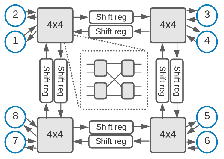
Figure 11: An 8$\times$8 mesh with eight endpoints and four routers. Each router is a 4$\times$4 butterfly and connects to two endpoints (shown as circles).

For this reason and in the interest of exploring different topologies, to scale up PaST-NoC, we can treat 4$\times$4 butterfly topologies as individual routers and, combined with our 2$\times$2 routers as additional building blocks, construct a variety of topologies of various scales and dimensions. One such example is a 2D mesh that has four routers arranged in a 2$\times$2 grid and a concentration factor of two. This topology can serve eight endpoints and thus we call it an 8$\times$8 2D mesh, shown in Figure 11. In this example, a deflection that occurs inside a butterfly manifests as a deflection at the mesh by a packet exiting a mesh router at an unexpected output. If that output leads to an endpoint, the deflected packet has to be re-injected into the NoC. Otherwise, the packet may proceed farther away from its destination but then has the opportunity to take hops towards its destination [16].

In this topology, we must delay packets between 4$\times$4 routers such that packets arrive at their next router at the beginning of an epoch. In contrast to the uni-directional butterfly, because the mesh is bi-directional, we cannot simply delay the periodic signals to some routers. Therefore, we add shift registers between routers. Those shift registers have a total delay of $E-P$ where $E$ is the duration of an epoch and $P$ is the propagation delay through a router (which is a 4$\times$4 butterfly). Each stage has a duration equal to the minimum spacing between data pulses ($SP$) that also defines the period of the clock input to each shift register similarly to Section IV-A. Therefore, each shift register has $\frac{E-P}{SP}$ stages. We reduce area overhead by using a flux-based shift register [37].

VI Evaluation

VI-A Methodology

We use a combination of Verilog, SPICE, a modified version of Booksim that implements deflection flow control [42, 16], and analytical models. We use a bottom–up approach where SPICE validates Verilog that validates Booksim models as scale increases. For SPICE and Verilog models, we build a library with the cells in Table I. For SPICE, we use the open-source MIT-LL SFQ5ee 10 kA/cm2 process and WRSPICE, an open source SPICE simulator. WRSPICE simulates our components at the circuit level. Our Verilog models emulate the behavior and approximate delays of each cell observed in SPICE. We use Verilog models beyond a single 2$\times$2 PaST-NoC router after which WRSPICE becomes impractical. Our WRSPICE decks include testbenches for which we use DC-RSFQ cells to take rectangular-like pulses as inputs and output RSFQ pulses which resemble a voltage spike. We use a supply and bias voltage of 10 mVs. In Verilog, in lieu of analog RSFQ spikes, we use 5ps long rectangular pulses to represent a pulse.

In both Verilog and WRSPICE, we confirm correct operation by testing all combinations of packets arriving to each input for any of the available destinations, or not arriving at all. We test each case with its own transient simulation as well as periodic repetition to test the round-robin function.

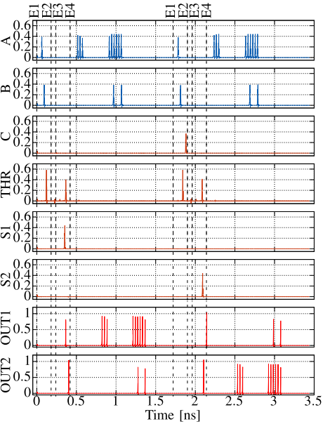
Figure 12: A 2$\times$2 PaST-NoC router implemented in WRSPICE. Two epochs are shown. Inputs are shown in blue ($A$ and $B$), internal pulses in orange ($C$, $Thr$, $S1$, and $S2$), and output pulses in red ($Out1$ and $Out2$).

To assign a data rate to our packets and compare against binary NoCs, we assume data pulses are encoded in RL. To evaluate throughput under high loads, we assume we try to send one pulse per data time slot with each pulse’s value determined with a uniform random probability. This mimics a binary NoC where packet length equals the size of the information endpoints send per packet. Therefore, we use Equation 1 to calculate how many data pulses each packet carries. We report bandwidth in gigabits per second (Gbps) per port after dividing it by the number of JJs of each NoC, in order to normalize performance per unit area. Reported throughput for PaST-NoC is only for packets that arrive to their intended destinations. Both our analytical models and Booksim implementation take into account multiple deflections of a single packet as well as deflections that occur due to previously deflected packets. Also, both models re-inject packets that are ejected from the NoC to an undesired destination due to a deflection.

We use detailed analytical models where accurate, in some cases augmented with Booksim simulations, to compare PaST-NoC against reported performance numbers from binary RSFQ NoCs due to the difficulty of implementing multiple designs in WRSPICE and in some cases the lack of detailed published information in the architecture or packet format to accurately re-implement binary NoCs. To explore the design space, we illustrate PaST-NoC’s throughput for different data period durations with a constant control period per packet, determined by the number of destinations. This is roughly equivalent to adjusting the payload size of a binary packet because it changes the control over data ratio. However, when comparing to prior binary NoCs, we cannot reliably vary their packet’s payload size for our evaluation based on available information. In fact, in some prior art control information is transmitted via separate wires; those designs are already at the data throughput-optimal point in terms of payload size because data transfer does not pause in order to transmit control information. Therefore, when evaluating PaST-NoC’s throughput for different data period durations, we do not adjust binary NoC data throughput.

VI-B Results

VI-B1 Timing Parameters

To preserve pulse count and integrity the minimum spacing of data pulses is 15ps. This guarantees that pulses will not overlap in any cell in the datapath and NDRO cells function correctly. Therefore, a data period of 300ps can fit at most $\frac{300}{15}=20$ data pulses. Additionally, the minimum duration of a time slot in the control period is 60ps. Therefore, in a PaST-NoC with two destinations, the control period lasts 180ps (two time slots plus one extra). Our WRSPICE circuit models include wires as inductors and parasitic inductance.

VI-B2 2$\times$2 Router

Figure 12 shows the round-robin deflection functionality of a 2$\times$2 PaST-NoC router in the case when two packets request the same output for two consecutive epochs. Packets arrive in each input and request output 1 since both packet’s control pulses arrive before $Thr$. In the first epoch, the packet from input $A$ is chosen as shown by a pulse in $S1$. In the second epoch, $C$ triggers and causes an $S2$ instead. Thus, the packet from input $B$ is chosen. In each epoch, the non-chosen packet is deflected to output 2. Data pulses of each packet follow the packet’s control pulse.

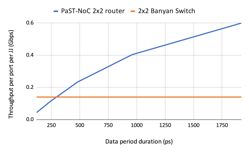
Figure 13: Throughput per port per JJ for a 2$\times$2 binary switch [11] and for a 2$\times$2 PaST-NoC router, as a function of the duration of a packet’s data period.

TABLE II: 2$\times$2 PaST-NoC router JJ count and delay breakdown.

Module	Number of JJs	Prop. delay (ps)
Conflict detection	27	40.95
Routing logic stage 1	87	50
Routing logic stage 2	91	41.06
Data crossbar	89	33.9
Resettable LA	34	28.95
Shift register	44	162.17
Miscellaneous	109	–
Summary	Total 481	In to out 213.41

Table II provides a breakdown of the number of JJs and propagation delay for different modules of a PaST-NoC router. We measure delay from the time the last input arrives to each module, until it produces its last output. We report the worst case delay (for different input patterns) for each module. “In to out” delay is the propagation delay through the router, from a packet first entering an input to starting to depart from an output. “Miscellaneous” refers to cells that are not explicitly assigned to a module, such as splitters and mergers that implement fanin and fanout. We notice a variability in the datapath of about $\pm$10ps due to the flux-based shift register. This variability can be drastically reduced with DFF-based shift registers but at a JJ cost. Lower variability can allow shorter control periods.

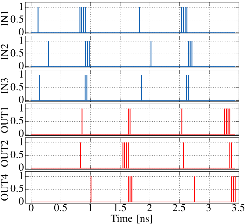
Figure 14: The 4$\times$4 PaST-NoC butterfly of Figure 10 implemented in Verilog. Two epochs are shown. Input pulses are shown in blue ($In1$, $In2$, $In3$) and output pulses in red ($Out1$, $Out2$, $Out3$).

In addition, we measure the static power of one PaST-NoC 2$\times$2 router to be 665.56$\mu$W, by measuring current draw. Worst case dynamic power, measured with a high frequency of pulses at a case where two incoming packets conflict is 195nW. Static power is much higher than dynamic power because our experiments are based on RSFQ technology that uses on-chip bias resistors that constantly consume power [1, 2]. To compare, we estimate the static power of the binary 2$\times$2 router of [11] from its schematic using the measured static power draw from individual cells in our library. The calculated static power is 1.4mW (approximately 2$\times$ that of a PaST-NoC router), including the clock tree that by itself consumes 15% more static power than a PaST-NoC router.

Figure 13 shows an analytical study of how average throughput per port per JJ varies in a 2$\times$2 PaST-NoC router as a function of the duration of the data period. This analysis is for uniform random (UR) traffic and includes the probability for a packet to be deflected, which is 25% for UR traffic. Doubling the data period does not double throughput, especially for longer data periods, because of the analysis of Equation 1. Note that for a single hop, there is no appreciable sustained data rate difference between a blocking NoC and PaST-NoC that re-injects deflected packets. For comparison, Figure 13 also includes calculated performance metrics for a 60-gate, 1184-JJ, 40GHz 2$\times$2 binary switch for a Banyan topology [11]. As shown, the crossover point is approximately a data period of 300ps.

VI-B3 4$\times$4 Butterfly

To implement the 4$\times$4 butterfly of Section VI-B3 that has 1924 JJs, we increase the control period by two time slots for a total of 300ps. We demonstrate the functionality using Verilog in Figure 14. As shown, packets from inputs 1 and 3 are both destined for destination 2 ($Out2$). Therefore, they conflict in router Ⓒ in the second column of Figure 10. In this example, input 1’s packet gets selected. Input 3’s packet gets deflected to destination 1. Also, in parallel, a packet from input 2 exits at destination 4 without causing any conflicts. In the next epoch, traffic repeats but router Ⓒ now deflects input 1’s packet to destination 1.

We then compare against two state of the art 4$\times$4 binary NoCs: (i) a 4$\times$4 Banyan topology with 4300 JJs [12] and (ii) a 4$\times$4 crossbar with 4316 JJs [8]. For each, we calculate performance metrics based on reported values. We also compare against a 4$\times$4 SRNoC router with 528 JJs and 64 time slots per connection window [27].

For PaST-NoC, we calculate average deflection rates and subsequently average throughput for the best case, UR, and worst case traffic. All other traffic patterns fall within this range. Best case traffic is one with no deflections. UR has a 25% deflection probability at every hop. Worst case traffic is one where in every first-stage router packets ask for the same output; therefore, packets have a 50% deflection probability at the first hop and then 25% at the second hop, since deflections help load balance [16]. For SRNoC, we compare the best case of PaST-NoC against the best case of SRNoC (UR) and the worst case of PaST-NoC against the worst case of SRNoC, which is a source sending at full rate to a single destination. All traffic patterns we evaluate are admissible, i.e., no destination receives more than 100% of traffic.

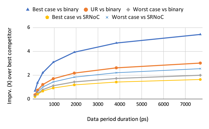
Figure 15: Improvement factor ($\times$) in throughput per port per JJ of a PaST-NoC 4$\times$4 butterfly as a function of a packet’s data period duration. Results are shown separately against SRNoC and the best of our two binary competitors.

Figure 15 shows the improvement factor ($\times$) in throughput per port per JJ of our 4$\times$4 PaST-NoC butterfly when compared to the best of the two aforementioned state of the art RSFQ binary NoCs with 4316 and 4781 JJs respectively, and separately when compared against SRNoC. An improvement factor of less than 1, equal to 1, or over 1 means that PaST-NoC has a lower, equal, or greater throughput per JJ compared to the best competitor, respectively. For the binary comparison, best case traffic has a crossover point of 450ps for the data period duration, UR has 930ps, and worst case traffic 1890ps. When compared to SRNoC, PaST-NoC’s worst case is more favorable because SRNoC’s worst case only uses a quarter of available bandwidth whereas PaST-NoC is a packet-switched NoC and thus adapts better to unbalanced traffic. For best traffic, the crossover point against SRNoC is 960ps and for worst case 465ps.

VI-B4 8$\times$8 Mesh

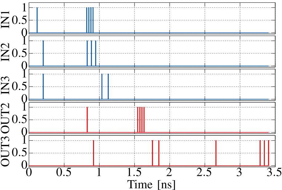
Figure 16: Verilog simulation of the 8$\times$8 2D mesh of Figure 11. Input pulses are shown in blue ($In1$, $In2$, $In3$) and output pulses in red ($Out2$, $Out3$).

Here we evaluate our 8$\times$8 2D mesh of Section V-B that has 7912 JJs. Figure 16 demonstrates its functionality in a case where three packets traverse the mesh. The packet from input 1 is destined to destination 2 ($Out2$). The packets from inputs 2 and 3 both are destined to destination 3. The packet from input 2 has a greater hop count because it travels from the top left 4$\times$4 router to the top right. Therefore, the two packets do not meet each other and exit at destination 3 in sequence with an empty epoch in between. This matches the behavior of a binary NoC with deflection flow control.

To evaluate throughput, we analytically calculate the total number of JJs including the inter-router shift registers. We then calculate the maximum throughput per port per JJ for PaST-NoC, assuming no deflections. To account for deflections, we use Booksim to simulate five synthetic traffic patterns using dimension order routing (DOR). In addition, we construct a synthetic traffic pattern that mimics temporal and spatial imbalance found in benchmarks. For each traffic pattern, we report the worst case (among all endpoints) percentage of the maximum throughput that an endpoint can achieve. We then use these percentages to scale down the throughput per port per JJ for PaST-NoC, compared to the maximum. In practice, benchmarks typically do not constantly inject at maximum throughput, thus their throughput is less penalized by deflections than what we report in our results for PaST-NoC. Booksim simulations use single-flit packets, which mimics PaST-NoC’s packets of the same length that propagate as a single unit. In addition, we scale up the control period to 540ps to address eight destinations.

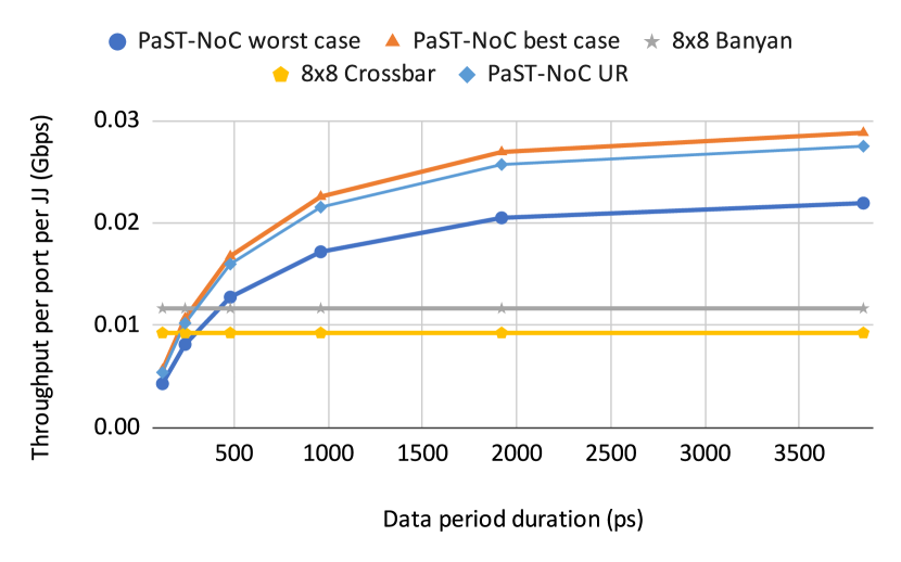
Figure 17: Throughput per port per JJ for the 8$\times$8 PaST-NoC mesh of Figure 11 as a function of the control period duration, an analytical model of an 8$\times$8 Banyan network constructed from 2$\times$2 switches [11], and an analytical model of an 8$\times$8 crossbar constructed from four 4$\times$4 crossbars [8].

For comparison, we analytically calculate throughput per port per JJ for (i) an 8$\times$8 binary Banyan NoC constructed from twelve 2$\times$2 switches [11] and (ii) an 8$\times$8 binary NoC constructed out of four 4$\times$4 crossbars [8] (the area of an N$\times$N fully-connected crossbar increases quadratically with $N$). For both competitors, the throughput per port of all admissible traffic patterns equals that of ideal traffic. However, throughput per port per JJ still is affected by the number of JJs.

Figure 17 shows that PaST-NoC outperforms both competitors for data periods longer than approximately 360ps for worst case traffic and 255ps for UR and best case traffic. The inter-router shift registers (Figure 11) have 42 to 290 stages each and collectively contribute 5% to 30% of the overall PaST-NoC JJ count, depending on the data period duration.

VI-B5 Scalability

The scales we study already approach the practical JJ count limits given RSFQ’s limited device density [1, 6], especially for chips that also contain memory elements. However, scaling up to more destinations favors binary NoCs because PaST-NoC’s control period scales linearly whereas a binary packet’s destination field scales logarithmically. Using analytical evaluations, with load balanced traffic PaST-NoC outperforms all binary RSFQ NoCs for up to a few hundred endpoints. Even under worst-case traffic and throughput assumptions, PaST-NoC remains favorable for a few tens of endpoints for long data periods. Deflection flow control has been shown to scale efficiently well within the scales we study [15, 16].

VI-B6 32$\times$32 Evaluation

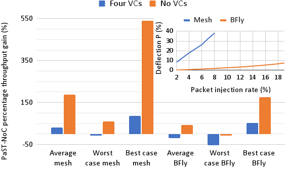
Figure 18: PaST-NoC throughput improvements as a percentage (%) for a 32$\times$32 concentrated 2D mesh with four endpoints per 8$\times$8 router, and a five-stage 32$\times$32 butterfly (BFly) with 2$\times$2 routers. The embedded graph (top right) shows in the Y axis the probability (%) for a packet to be deflected in an 8$\times$8 router in the mesh network or a $2\times$2 router in the butterfly network, by average across our traffic patterns. The X axis shows the packet injection rate (%) until the first pattern saturates in each of the two PaST-NoC topologies.

We scale up our throughput evaluation to 32 inputs and 32 outputs using a modified version of Booksim that simulates deflection flow control [16]. We simulate two topologies: (i) a 2D concentrated mesh with four terminals per router (routers are 8$\times$8), and (ii) a five-stage butterfly with 2$\times$2 routers. For the mesh, we design an 8$\times$8 PaST-NoC router from a three-stage butterfly. We compare PaST-NoC against a buffered NoC with credit-based flow control and either no virtual channels (one buffer per input) or four VCs to show a higher-performing variation. The no VC case matches previously-demonstrated RSFQ binary NoCs. The butterfly uses destination tag single-path routing while the no VC mesh DOR. For four VCs in the mesh, we keep the highest throughput among deterministic DOR, oblivious XY-YX routing, and minimal adaptive [42]. We adjust the throughput per port for PaST-NoC based on our average results for 1000ps data periods from Figure 17 and Figure 15, as well as the control period scaling characteristics of Section VI-B5. We use cycle times that are based on simple RSFQ NoCs without VCs for all buffered cases in Booksim, even though VCs increase complexity thus prolonging the critical path. We also assume all buffered routers have one pipeline stage and ignore additional area to implement VCs. All these assumptions favor the buffered case. Figure 18 shows the throughput for the PaST-NoC average, best, and worst case over five synthetic traffic patterns: UR, tornado, bitcomp, shuffle, and transpose [42].

As shown, PaST-NoC outperforms the no VC buffered case by an average 188% for the mesh and 43% for the butterfly. The best case for PaST-NoC for the mesh is for the tornado traffic pattern where deflection acts to load balance traffic better than any of our three routing policies in the buffered case. For the butterfly, the worst case for PaST-NoC is UR traffic where transient imbalance can cause a deflection in any of the five hops. In that case, because the butterfly is not bi-directional and has no path diversity, even a single deflection forces the packet to fully exit and re-enter the network; in the mesh a single deflection just costs two hops (Section V-B). PaST-NoC outperforms the four VC case in half the metrics, and the no VC case in all experiments except for one traffic pattern in the butterfly where PaST-NoC shows a 7% penalty.

Figure 18 also shows the per-packet PaST-NoC deflection probability. Furthermore, we notice that even though latency increases more rapidly with injection rate than buffered NoCs [16, 15], the higher bandwidth of PaST-NoC results in lower network load for a constant bits per second of injection rate. Therefore, in test cases where PaST-NoC outperforms buffered NoCs, the latency impact of deflection is below 2% for injection rates that do not saturate the buffered NoCs.

VI-C CMOS Comparison

Using energy-efficient RSFQ (ERSFQ) [43] we can eliminate static power consumption. We can also account for the power associated with cooling by multiplying the circuit power by 400$\times$ [44]. In this case, based on our JJ count and power results from Section VI-B2, dynamic power for a 2$\times$2 PaST-NoC router becomes a few $\mu$W. Specifically, including the cooling overhead, our 195nW measurement for worst-case dynamic power becomes $195nW\times 400=78\mu$W. In an “average” case where only one packet traverses the 2$\times$2 router, dynamic power is approximately half of that. Even with a 50% dynamic power penalty to account for ERSFQ’s multiplicative power overhead relative to pure logic components [45], worst-case total power for one 2$\times$2 PaST-NoC router remains below 150 $\mu$W. This number is a few orders of magnitude lower than the mW typically reported in modern CMOS NoCs. For instance, DDRNoC and ArSMART report one to eight W total for an $8\times 8$ 2D mesh depending on load [46, 47]. This results in approximately 10-150 mW (67$\times$ to 1000$\times$ higher) per router for both CMOS NoCs.

Comparing throughput between CMOS NoCs and PaST-NoC depends on multiple parameters. Under low enough injected load, all NoCs satisfy injected traffic thus provide the same throughput. Therefore, PaST-NoCs provides higher throughput per power because it reduces power as explained above assuming ERSFQ. Using as an example our $32\times 32$ 2D mesh of Section VI-B6 under UR traffic, DDRNoC [46] has an approximately 10$\times$ higher maximum throughput (Gbps) per port than PaST-NoC, assuming 16 time slots per packet and the analysis of Equation 1. However, even after taking into account the best case router power numbers for CMOS NoCs, PaST-NoC provides $6.7\times$ higher throughput per unit power. This analysis only takes into account router power, but including wire power will make the final result more favorable for PaST-NoC due to the high power contribution of wires in CMOS NoCs [16], which is significantly lower in RSFQ [48].

Finally, if we use JJ area models for a modern manufacturing process, a 2$\times$2 PaST-NoC router occupies approximately a few hundredths of $mm^{2}$. Even with a 3$\times$ area penalty for non-JJ components, routing, and layout, PaST-NoC occupied area is on par with modern CMOS NoCs despite the stark device density difference.

VII Discussion and Future Work

High timing variability may necessitate more conservative pulse spacing or prolonging control periods and time slots. In the future, we can investigate variable-length epochs or coalescing packets to support variable-size packets. We can also investigate zero-payload packets; this can support the creation of circuits or channel reservations. While we can design larger-scale versions of a butterfly and a mesh, PaST-NoC can also construct numerous other topologies such as a fat tree and a torus by using the same building blocks. Finally, shift registers within and across routers are just retiming elements, similar to pipeline DFFs in CMOS; packets do not stall in shift registers or elsewhere in PaST-NoC, and thus cannot deadlock.

VIII Conclusion

We propose PaST-NoC, a packet-switched superconducting NoC with deflection flow control that operates its control path using RL, addressing the stringent area constraints of superconducting technology. PaST-NoC packets carry data pulses that receivers can interpret as pulse trains, RL, serialized binary, or other formats. PaST-NoC scales to arbitrary topologies based on 2$\times$2 routers and 4$\times$4 butterflies. PaST-NoC outperforms binary RSFQ NoCs by as much as over $5\times$.

References

- [1] S. S. Tannu, P. Das, M. L. Lewis, R. Krick, D. M. Carmean, and M. K. Qureshi, “A case for superconducting accelerators,” ser. CF, 2019.
- [2] V. Michal, E. Baggetta, M. Aurino, S. Bouat, and J. Villegier, “Superconducting RSFQ logic: Towards 100GHz digital electronics,” in Proceedings of 21st International Conference Radioelektronika, 2011.
- [3] N. Yoshikawa, H. Tago, and K. Yoneyama, “A new design approach for RSFQ logic circuits based on the binary decision diagram,” IEEE Transactions on Applied Superconductivity, vol. 9, no. 2, 1999.
- [4] G. Krylov and E. G. Friedman, “Asynchronous dynamic single-flux quantum majority gates,” IEEE Transactions on Applied Superconductivity, vol. 30, no. 5, pp. 1–7, 2020.
- [5] G. Tzimpragos, D. Vasudevan, N. Tsiskaridze, G. Michelogiannakis, A. Madhavan, J. Volk, J. Shalf, and T. Sherwood, “A computational temporal logic for superconducting accelerators,” ser. ASPLOS, 2020.
- [6] S. Tolpygo, “Superconductor digital electronics: Scalability and energy efficiency issues,” vol. 42, pp. 463–485, 05 2016.
- [7] F. Zokaee and L. Jiang, “SMART: A heterogeneous scratchpad memory architecture for superconductor SFQ-based systolic CNN accelerators,” MICRO-54: 54th Annual IEEE/ACM International Symposium on Microarchitecture, Oct 2021. [Online]. Available: http://dx.doi.org/10.1145/3466752.3480041
- [8] S. Yorozu, Y. Hashimoto, Y. Kameda, H. Terai, A. Fujimaki, and N. Yoshikawa, “A 40 GHz clock 160 Gb/s 4/spl times/4 switch circuit using single flux quantum technology for high-speed packet switching systems,” ser. HPSR, 2004.
- [9] T. Yamada, M. Yoshida, T. Hanai, A. Fujimaki, H. Hayakawa, Y. Kameda, S. Yorozu, H. Terai, and N. Yoshikawa, “Quantitative evaluation of the single-flux- quantum cross/bar switch,” IEEE Transactions on Applied Superconductivity, vol. 15, no. 2, 2005.
- [10] A. H. Worsham, J. X. Przybysz, Joonhee Kang, and D. L. Miller, “A single flux quantum cross-bar switch and demultiplexer,” IEEE Transactions on Applied Superconductivity, vol. 5, no. 2, 1995.
- [11] Y. Kameda, S. Yorozu, and S. Tahara, “SFQ standard cell-based circuit design of an internal link speeded-up batcher-banyan packet switch,” Applied Superconductivity, IEEE Tran. on, vol. 11, 2001.
- [12] L. Wittie, D. Y. Zinoviev, G. Sazaklis, and K. Likharev, “CNET: design of an RSFQ switching network for petaflops-scale computing,” IEEE Transactions on Applied Superconductivity, vol. 9, no. 2, 1999.
- [13] S. Yorozu, Y. Hashimoto, H. Numata, M. Koike, M. Tanaka, and S. Tahara, “Full operation of a three-node pipeline-ring switching chip for a superconducting network system,” IEEE Transactions on Applied Superconductivity, vol. 9, no. 2, pp. 3590–3593, 1999.
- [14] Y. Kameda, S. Yorozu, Y. Hashimoto, H. Terai, A. Fujimaki, and N. Yoshikawa, “Single-flux-quantum (SFQ) circuit design and test of crossbar switch scheduler,” IEEE Transactions on Applied Superconductivity, vol. 15, no. 2, 2005.
- [15] T. Moscibroda and O. Mutlu, “A case for bufferless routing in on-chip networks,” ser. ISCA ’09, 2009, p. 196–207.
- [16] G. Michelogiannakis, D. Sanchez, W. J. Dally, and C. Kozyrakis, “Evaluating bufferless flow control for on-chip networks,” in 2010 Fourth ACM/IEEE International Symposium on Networks-on-Chip, 2010.
- [17] O. A. Mukhanov, “Energy-efficient single flux quantum technology,” IEEE Transactions on Applied Superconductivity, vol. 21, no. 3, pp. 760–769, 2011.
- [18] C. R. Jesshope, P. R. Miller, and J. T. Yantchev, “High performance communications in processor networks,” ser. ISCA ’89. ACM, 1989, p. 150–157.
- [19] S. Konstantinidou and L. Snyder, “The chaos router: A practical application of randomization in network routing,” SIGARCH Comput. Archit. News, vol. 19, no. 1, p. 79–88, mar 1991. [Online]. Available: https://doi.org/10.1145/121956.121965
- [20] P. Gonzalez-Guerrero, M. G. Bautista, D. Lyles, and G. Michelogiannakis, “Temporal and SFQ pulse-streams encoding for area-efficient superconducting accelerators,” in Proceedings of the 27th ACM International Conference on Architectural Support for Programming Languages and Operating Systems, ser. ASPLOS 2022. New York, NY, USA: Association for Computing Machinery, 2022, p. 963–976. [Online]. Available: https://doi.org/10.1145/3503222.3507765
- [21] G. Bautista, P. Gonzalez-Guerrero, D. Lyles, K. Huch, and G. Michelogiannakis, “Superconducting digital DIT butterfly unit for fast Fourier transform using race logic,” in 2022 20th IEEE Interregional NEWCAS Conference (NEWCAS), 2022, pp. 441–445.
- [22] Y. Ueno, M. Kondo, M. Tanaka, Y. Suzuki, and Y. Tabuchi, “QECOOL: On-line quantum error correction with a superconducting decoder for surface code,” in 2021 58th ACM/IEEE Design Automation Conference (DAC), 2021, pp. 451–456.
- [23] A. Bozbey, M. A. Karamuftuoglu, S. Razmkhah, and M. Ozbayoglu, “Single flux quantum based ultrahigh speed spiking neuromorphic processor architecture,” 2018. [Online]. Available: https://arxiv.org/abs/1812.10354
- [24] R. McDermott, M. G. Vavilov, B. L. T. Plourde, F. K. Wilhelm, P. J. Liebermann, O. A. Mukhanov, and T. A. Ohki, “Quantum–classical interface based on single flux quantum digital logic,” Quantum Science and Technology, vol. 3, no. 2, p. 024004, jan 2018. [Online]. Available: https://doi.org/10.1088/2058-9565/aaa3a0
- [25] M. A. Karamuftuoglu and A. Bozbey, “Ultrahigh speed artificial neuron compatible with standard foundry processes and SFQ cells,” CoRR, vol. abs/1812.10354, 2018.
- [26] A. Bozbey, M. A. Karamuftuoglu, S. Razmkhah, and M. Ozbayoglu, “Single flux quantum based ultrahigh speed spiking neuromorphic processor architecture,” 2020.
- [27] G. Michelogiannakis, D. Lyles, P. Gonzalez-Guerrero, M. Bautista, D. Vasudevan, and A. Butko, “SRNoC: A statically-scheduled circuit-switched superconducting race logic NoC,” in IPDPS, 2021.
- [28] V. Kaplunenko, M. Khabipov, D. Khokhlov, A. Kirichenko, V. Koshelets, and S. Kovtonyuk, “Experimental implementation of SFQ NDRO cells and 8-bit ADC,” IEEE Transactions on Applied Superconductivity, 1993.
- [29] P. Russer, “General energy relations for josephson junctions,” Proceedings of the IEEE, vol. 59, no. 2, pp. 282–283, 1971.
- [30] G. Krylov and E. G. Friedman, Single Flux Quantum Integrated Circuit Design. Springer, 2022.
- [31] T. Jabbari, E. G. Friedma, and J. Kawa, “H-tree clock synthesis in RSFQ circuits,” in 2020 17th Biennial Baltic Electronics Conference (BEC), 2020, pp. 1–5.
- [32] A. Madhavan, T. Sherwood, and D. Strukov, “Race logic: A hardware acceleration for dynamic programming algorithms,” SIGARCH Comput. Archit. News, vol. 42, no. 3, p. 517–528, Jun. 2014.
- [33] W. J. Dally and B. Towles, “Route packets, not wires: On-chip inteconnection networks,” ser. DAC, 2001.
- [34] M. Horro, G. Rodríguez, and J. Touriño, “Simulating the network activity of modern manycores,” IEEE Access, vol. 7, pp. 81 195–81 210, 2019.
- [35] S. M. Tam, H. Muljono, M. Huang, S. Iyer, K. Royneogi, N. Satti, R. Qureshi, W. Chen, T. Wang, H. Hsieh, S. Vora, and E. Wang, “Skylake-sp: A 14nm 28-core xeon® processor,” in 2018 IEEE International Solid - State Circuits Conference - (ISSCC), 2018, pp. 34–36.
- [36] M. Mishkin, N. S. Kim, and M. Lipasti, “Temporal codes in on-chip interconnects,” ser. ISLPED, 2017.
- [37] M. G. Bautista, P. Gonzalez-Guerrero, D. Lyles, and G. Michelogiannakis, “Superconducting shuttle-flux shift buffer for race logic,” in MWSCAS, 2021, pp. 796–801.
- [38] A. Kidiyarova-Shevchenko and D. Zinoviev, “RSFQ pseudo random generator and its possible applications,” IEEE Transactions on Applied Superconductivity, vol. 5, no. 2, pp. 2820–2822, 1995.
- [39] D. B. Rita Mahajan, Komal Devi, “Review on standard and multibit linear feedback shift register,” in JETIR, 2019.
- [40] X. Zhou, S. Xu, P. Rott, C. Mancini, and M. Feldman, “50 GHz RSFQ pseudo-random number generator design,” IEEE Transactions on Applied Superconductivity, vol. 11, no. 1, pp. 617–620, 2001.
- [41] A. Choudhury and V. Li, “Effect of contention resolution rules on the performance of deflection routing,” in IEEE Global Telecommunications Conference GLOBECOM ’91: Countdown to the New Millennium. Conference Record, 1991, pp. 1706–1711 vol.3.
- [42] N. Jiang, D. U. Becker, G. Michelogiannakis, J. Balfour, B. Towles, D. E. Shaw, J. Kim, and W. J. Dally, “A detailed and flexible cycle-accurate network-on-chip simulator,” in 2013 IEEE International Symposium on Performance Analysis of Systems and Software (ISPASS), April 2013, pp. 86–96.
- [43] O. A. Mukhanov, “Energy-efficient single flux quantum technology,” IEEE Transactions on Applied Superconductivity, vol. 21, no. 3, pp. 760–769, 2011.
- [44] K. Ishida, I. Byun, I. Nagaoka, K. Fukumitsu, M. Tanaka, S. Kawakami, T. Tanimoto, T. Ono, J. Kim, and K. Inoue, “SuperNPU: An extremely fast neural processing unit using superconducting logic devices,” in 2020 53rd Annual IEEE/ACM International Symposium on Microarchitecture (MICRO). IEEE, 2020, pp. 58–72.
- [45] N. K. Katam, O. Mukhanov, and M. Pedram, “Simulation analysis and energy-saving techniques for ERSFQ circuits,” IEEE Transactions on Applied Superconductivity, vol. 29, no. 5, pp. 1–7, 2019.
- [46] A. Ejaz, V. Papaefstathiou, and I. Sourdis, “DDRNoC: Dual data-rate network-on-chip,” ACM Trans. Archit. Code Optim., vol. 15, no. 2, jun 2018. [Online]. Available: https://doi.org/10.1145/3200201
- [47] H. Chen, P. Chen, J. Zhou, L. H. K. Duong, and W. Liu, “ArSMART: An improved smart noc design supporting arbitrary-turn transmission,” IEEE Transactions on Computer-Aided Design of Integrated Circuits and Systems, vol. 41, no. 5, pp. 1316–1329, 2022.
- [48] T. Jabbari, G. Krylov, S. Whiteley, E. Mlinar, J. Kawa, and E. G. Friedman, “Interconnect routing for large-scale RSFQ circuits,” IEEE Transactions on Applied Superconductivity, vol. 29, no. 5, pp. 1–5, 2019.