Modelling Emotion Dynamics in Song Lyrics with State Space Models

Abstract

Most previous work in music emotion recognition assumes a single or a few song-level labels for the whole song. While it is known that different emotions can vary in intensity within a song, annotated data for this setup is scarce and difficult to obtain. In this work, we propose a method to predict emotion dynamics in song lyrics without song-level supervision. We frame each song as a time series and employ a State Space Model (SSM), combining a sentence-level emotion predictor with an Expectation-Maximization (EM) procedure to generate the full emotion dynamics. Our experiments show that applying our method consistently improves the performance of sentence-level baselines without requiring any annotated songs, making it ideal for limited training data scenarios. Further analysis through case studies shows the benefits of our method while also indicating the limitations and pointing to future directions.

1 Introduction

Music and emotions are intimately connected, with almost all music pieces being created to express and induce emotions (Juslin and Laukka, 2004). As a key factor of how music conveys emotion, lyrics contain part of the semantic information that the melodies cannot express (Besson et al., 1998). Lyrics-based music emotion recognition has attracted increasing attention driven by the demand to process massive collections of music tracks automatically, which is an important task to streaming and media service providers (Kim et al., 2010; Malheiro et al., 2016; Agrawal et al., 2021).

Most emotion recognition studies in Natural Language Processing (NLP) assume the text instance expresses a static and single emotion (Mohammad and Bravo-Márquez, 2017; Nozza et al., 2017; Mohammad et al., 2018a). However, emotion is non-static and highly correlated with the contextual information, which makes the single-label assumption too simplistic in dynamic scenarios, not just in music (Schmidt and Kim, 2011) but also in other domains such as conversations (Poria et al., 2019b). Figure 1 shows an example of this dynamic behaviour, where the intensities of three different emotions vary within a song. Accurate emotion recognition systems should ideally be able to generate the full emotional dynamics for each song, as opposed to simply predicting a single label.

A range of datasets and corpora for modelling dynamic emotion transitions has been developed in the literature (McKeown et al., 2011; Li et al., 2017; Hsu et al., 2018; Poria et al., 2019a; Firdaus et al., 2020), but most of them do not use song lyrics as the domain and assume discrete, categorical labels for emotions (either the presence or absence of one emotion). To the best of our knowledge, the dataset from Mihalcea and Strapparava (2012) is the only one that provides full fine-grained emotion intensity annotations for song lyrics at the verse level. The lack of large-scale datasets for this task poses a challenge for traditional supervised methods. While previous work proposed methods for the similar sequence-based emotion recognition task, they all assume the availability of some levels of annotated data at training time, from full emotion dynamics (Kim et al., 2015) to coarse, discrete document-level labels (Täckström and McDonald, 2011b).

The data scarcity problem motivates our main research question: “Can we predict emotion dynamics in song lyrics without requiring annotated lyrics?”. In this work, we claim that the answer is affirmative. To show this, we propose a method consisting of two major stages: (1) a sentence or verse-level regressor that leverages existing emotion lexicons, pre-trained language models and other sentence-level datasets and (2) a State Space Model (SSM) that constructs a full song-level emotional dynamics given the initial verse-level scores. Intuitively, we treat each verse as a time step and the emotional intensity sequence as a latent time series that is inferred without any song-level supervision, directly addressing the limited data problem. To the best of our knowledge, this scenario was never addressed before either for song lyrics or other domains.

To summarize, our main contributions are:

• We propose a hybrid approach for verse-level emotion intensity prediction that combines emotion lexicons with a pre-trained language model (BERT (Devlin et al., 2019) used in this work), which is trained on available sentence-level data.

• We further show that by using SSMs to model the song-level emotion dynamics, we can improve the performance of the verse-level approach without requiring any annotated lyrics.

• We perform a qualitative analysis of our best models, highlighting its limitations and pointing to directions for future work.

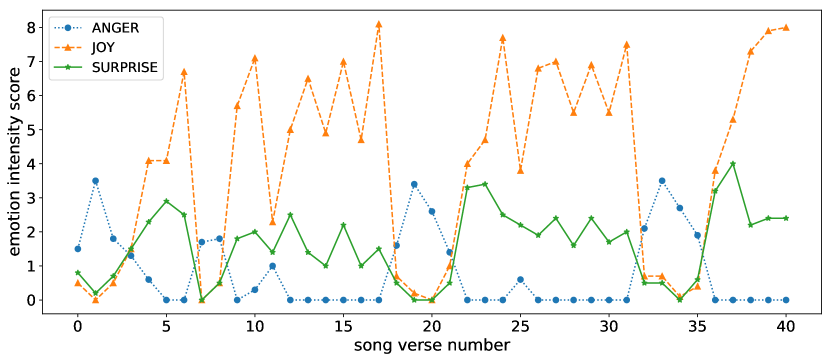
Figure 1: An illustration of emotion dynamics of a song in the LyricsEmotions dataset of Mihalcea and Strapparava (2012). Note the intensities of each emotion vary from verse to verse within the song.

2 Background and Related Work

Emotion Models.

Human emotion is a long-standing research field in psychology, with many studies aiming at defining a taxonomy for emotions. In NLP, emotion analysis mainly employs the datasets which are annotated based on the categorical or the dimensional model.

The categorical model assumes a fixed set of discrete emotions which can vary in intensity. Emotions can overlap but are assumed to be separate “entities” for each other, such as anger, joy and surprise. Taxonomies using the categorical model include Ekman’s basic emotions (Ekman, 1993) and Plutchik’s wheel of emotions (Plutchik, 1980). The dimensional models place emotions in a continuous space: the VAD (Valence, Arousal and Dominance) taxonomy of Russell (1980) is the most commonly used in NLP. In this work, we focus on the Ekman taxonomy for purely experimental purposes, as it is the one used in the available data we employ. However, our approach is general and could be applied to other taxonomies.

Dynamic Emotion Analysis.

Emotion Recognition in Conversation (ERC) (Poria et al., 2019b), which focuses on tracking dynamic shifts of emotions, is the most similar task to our work. Within a conversation, the emotional state of each utterance is influenced by the previous state of the party and the stimulation from other parties (Li et al., 2020; Ghosal et al., 2021). Such an assumption of the real-time dynamic emotional changes also exists in music: the affective state of the current lyrics verse is correlated with the state of the previous verse(s) as a song progresses.

Contextual information in the ERC task is generally captured by deep learning models, which can be roughly categorized into sequence-based and graph-based methods (Hu et al., 2021). Sequence-based methods encode conversational context features using established methods like Recurrent Neural Networks (Poria et al., 2017; Hazarika et al., 2018a, b; Majumder et al., 2019; Hu et al., 2021) and Transformer-based architectures (Zhong et al., 2019; Li et al., 2020). They also include more advanced and tailored methods like Hierarchical Memory Network (Jiao et al., 2020), Emotion Interaction Network (Lu et al., 2020) and Causal Aware Network (Zhao et al., 2022). Graph-based methods apply specific graphical structures to model dependencies in conversations (Ghosal et al., 2019; Zhang et al., 2019; Lian et al., 2020; Ishiwatari et al., 2020; Shen et al., 2021) by utilizing Graph Neural Networks (Kipf and Welling, 2017). In contrast to these methods, we capture contextual information using a State Space Model, mainly motivated by the need for a method that can train without supervision. Extending and/or combining an SSM with a deep learning model is theoretically possible but non-trivial, and care must be taken in a low-data situation such as ours.

The time-varying nature of music emotions has been investigated in music information retrieval (Caetano et al., 2012). To link the human emotions with the music acoustic signal, the emotion distributions were modelled as 2D Gaussian distributions in the Arousal-Valence (A-V) space, which were used to predict A-V responses through multi-label regression (Schmidt et al., 2010; Schmidt and Kim, 2010). Building on previous studies, Schmidt and Kim (2011) applied structured prediction methods to model complex emotion-space distributions as an A-V heatmap. These studies focus on the mapping between emotions and acoustic features/signals, while our work focuses on the lyrics component. Wu et al. (2014) developed a hierarchical Bayesian model that utilized both acoustic and textual features, but it was only applied to predict emotions as discrete labels (presence or absence) instead of fine-grained emotion intensities as in our work.

Combining pre-trained Language Models with External Knowledge.

Pre-trained language models (LMs) including BERT (Devlin et al., 2019), XLNet (Yang et al., 2019) and GPT (Brown et al., 2020) have achieved state-of-the-art performance in numerous NLP tasks. Considerable effort has been made towards combining context-sensitive features of LMs with factual or commonsense knowledge from structured sources, including domain-specific knowledge (Ying et al., 2019), structured semantic information (Zhang et al., 2020), language-specific knowledge (Alghanmi et al., 2020; De Bruyne et al., 2021) and linguistic features (Koufakou et al., 2020; Mehta et al., 2020). This auxiliary knowledge is usually infused into the architecture by concatenating them with the Transformer-based representation before the prediction layer for downstream tasks. Our method proposes to utilize the rule-based representations derived from a bunch of affective lexicons to improve the performance of BERT by incorporating task-specific knowledge. The motivation for our proposal is the hypothesis that the extension of lexicon-based information will compensate for BERT’s lack of proper representations of semantic and world knowledge (Rogers et al., 2021), making the model more stable across domains.

State Space Models.

In NLP tasks such as Part-of-Speech (POS) tagging and Named Entity Recognition, contextual information is widely acknowledged to play an important role in prediction. This leads to the adoption of structured prediction approaches such as Hidden Markov Model (HMM) (Rabiner and Juang, 1986), Maximum Entropy Markov Model (MEMM) (McCallum et al., 2000) and Conditional Random Field (CRF) (Lafferty et al., 2001), which relate a set of observable variables to a set of latent variables (e.g., words and their POS tags). State Space Models (SSMs) are similar to HMMs but assume continuous variables. Linear Gaussian SSM (LG-SSM) is a particular case of SSM in which all the conditional probability distributions are linear and Gaussian.

Following the notation from Murphy (2012, Chap. 18), we briefly introduce the LG-SSM that we employ in our work. LG-SSMs assume a sequence of observed variables $\mathbf{y}_{1:T}$ as input, and the goal is to draw inferences about the corresponding hidden states $\mathbf{z}_{1:T}$, where $T$ is the length of the sequence. Their relationship is given at each step $t$ by the equations as:

$$\mathbf{z}_{t} =\mathbf{A}\mathbf{z}_{t-1}+\epsilon_{t}, \epsilon_{t}\sim{\mathcal{N}}\left(0,\mathbf{Q}\right)$$

$$\mathbf{y}_{t} =\mathbf{C}\mathbf{z}_{t}+\delta_{t}, \delta_{t}\sim{\mathcal{N}}\left(0,\mathbf{R}\right)$$

where $\Theta=(\mathbf{A},\mathbf{C},\mathbf{Q},\mathbf{R})$ are the model parameters, $\epsilon_{t}$ is the system noise and $\delta_{t}$ is the observation noise. The equations above are also referred as transition and observation equations, respectively. Given $\Theta$ and a sequence $\mathbf{y}_{1:T}$, the goal is to obtain the posteriors $p(\mathbf{z}_{t})$ for each step $t$. In an LG-SSM, this posterior is a Gaussian and can be obtained in closed form by applying the celebrated Kalman Filter (Kalman, 1960) .

There exist some other latent variable models to estimate temporal dynamics of emotions and sentiments in product reviews (McDonald et al., 2007; Täckström and McDonald, 2011a, b) and blogs (Kim et al., 2015). McDonald et al. (2007) and Täckström and McDonald (2011a, b) combined document-level and sentence-level supervision as the observed variables to condition on the latent sentence-level sentiment. Kim et al. (2015) introduced a continuous variable $\mathbf{y}_{t}$ to solely determine the sentiment polarity $\mathbf{z}_{t}$, while $\mathbf{z}_{t}$ is conditioned on both $\mathbf{y}_{t}$ and $\mathbf{z}_{t-1}$ for each $t$ in the LG-SSM.

3 Method

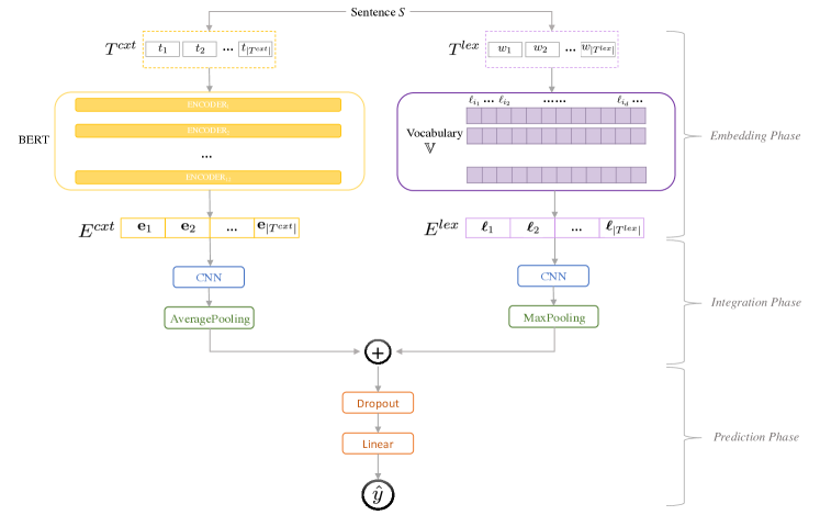
Figure 2: BERTLex architecture used for the verse-level model.

We propose a two-stage method to predict emotion dynamics without requiring annotated song lyrics. The first stage is a verse-level model that predicts initial scores for each song verse, where we use a hybrid approach combining lexicons and sentence-level annotated data from a different domain (section 3.1). The second stage contextualizes these scores in the entire song, incorporating them into an LG-SSM trained in an unsupervised way (section 3.2).

Task Formalization.

Let $d_{x}^{y}$ indicate the real-valued intensity of emotion $y$ for sentence/ verse $x$, where $x\in\mathcal{X}$ and $y\in\mathcal{Y}$. Note that $\mathcal{Y}$ = $\{y_{1},y_{2},\dots,y_{c}\}$ is a set of $c$ labels, each of which represents one of the basic emotions ($c$ = 6 for the datasets we used). Given a source dataset $\mathbb{D}_{s}$ = $\{(x_{1},E_{1}),(x_{2},E_{2}),\dots,(x_{M},E_{M})\}$, where $x_{i}$ is a sentence, $E_{i}$ = $\{d_{x_{i}}^{y_{1}},d_{x_{i}}^{y_{2}},\dots,d_{x_{i}}^{y_{c}}\}$ and $M$ = $|\mathbb{D}_{s}|$. The target dataset is $\mathbb{D}_{t}$ = $\{S_{1},S_{2},\dots,S_{|\mathbb{D}_{t}|}\}$, where $|\mathbb{D}_{t}|$ is the number of sequences (i.e., songs) and $S_{i}$ = $\{(v_{1},E_{1}),(v_{2},E_{2}),\dots,(v_{|S_{i}|},E_{|S_{i}|})\}$ is a song consisting of $|S_{i}|$ verses. In the song $S_{i}$, the $j$-th verse $v_{j}$ is also associated with $c$ emotion intensities as $E_{j}$ = $\{d_{v_{j}}^{y_{1}},d_{v_{j}}^{y_{2}},\dots,d_{v_{j}}^{y_{c}}\}$. Given the homogeneity of label spaces of $\mathbb{D}_{s}$ and $\mathbb{D}_{t}$, the model trained by using $\mathbb{D}_{s}$ can be applied to predict for $\mathbb{D}_{t}$ directly. The output of verse-level model is the emotion intensity predictions $\hat{\mathbf{Y}}\in\mathbb{R}^{N\times c}$, where $N$ is the total number of verses in $\mathbb{D}_{t}$. Finally, we use $\hat{\mathbf{Y}}$ as the input sequences of the song-level model to produce optimized emotion intensity sequences $\hat{\mathbf{Z}}\in\mathbb{R}^{|\mathbb{D}_{t}|\times c}$.

3.1 Verse-Level Model

Emotion lexicons provide information on associations between words and emotions (Ramachandran and de Melo, 2020), which are proven to be beneficial in recognising textual emotions (Mohammad et al., 2018b; Zhou et al., 2020). Given that we would like to acquire accurate initial predictions at the verse level, we opted for a hybrid methodology that combines learning-based and lexicon-based approaches to enhance feature representation.

Overview.

The verse-level model architecture is called BERTLex, as illustrated in Figure 2. The BERTLex model consists of three phases: (1) the embedding phase, (2) the integration phase, and (3) the prediction phase. In the embedding phase, the input sequence is represented as both contextualized embeddings from BERT and static word embeddings from lexicons. In the integration phase, contextualized and static word embeddings are concatenated at the sentence level by taking the pooling operations on the two embeddings separately. The prediction phase encodes the integrated sequence of feature vectors and performs the verse-level emotion intensity regression by using the $\mathbb{D}_{s}$ as the training/development set and the $\mathbb{D}_{t}$ as the test set.

Embedding Phase.

The input sentence $S$ is tokenized in two ways: one for the pre-trained language model and the other for the lexicon-based word embedding. These two tokenized sequences are denoted as $T^{cxt}$ and $T^{lex}$, respectively. Then, $T^{cxt}$ is fed into the pre-trained BERT to produce a sequence of contextualized word embeddings $E^{cxt}=\{\mathbf{e}_{1},\mathbf{e}_{2},\ldots,\mathbf{e}_{|T^{cxt}|}\}$, where $E^{cxt}\in\mathbb{R}^{|T^{cxt}|\times D_{cxt}}$ and $D_{cxt}$ is the embedding vector dimension.

To capture task-specific information, a Lexicon embedding layer encodes a sequence of emotion and sentiment word associations for $T^{lex}$, generating a sequence of lexicon-based embeddings $E^{lex}=\{{\boldsymbol{\ell}}_{1},{\boldsymbol{\ell}}_{2},\ldots,{\boldsymbol{\ell}}_{|T^{lex}|}\}$, where $E^{lex}\in\mathbb{R}^{|T^{lex}|\times D_{lex}}$ and $D_{lex}$ is the lexical embedding vector dimension. We first build the vocabulary $\mathbb{V}$ from the text of $\mathbb{D}_{s}$ and $\mathbb{D}_{t}$. For each word $\mathbf{v}_{i}$ in $\mathbb{V}$ of $T^{lex}$, we use $d$ lexicons to generate the rule-based feature vectors ${\boldsymbol{\ell}}_{i}$ = {$\ell_{i_{1}},\ell_{i_{2}},\ldots,\ell_{i_{d}}$}, where $\ell_{i_{j}}$ is the lexical feature vector for word $\mathbf{v}_{i}$ derived from the $j$-th lexicon and $D_{lex}$ = $|{\boldsymbol{\ell}}_{i}|$. Additionally, we perform a degree-$p$ polynomial expansion on the feature vector $\ell_{i_{j}}$.

Integration Phase.

As BERT uses the WordPiece tokenizer (Wu et al., 2016) to split a number of words into a sequence of subwords, the contextualized embedding cannot be directly concatenated with the different-size static word embedding. Inspired by Alghanmi et al. (2020), we combine the contextualized embeddings and static word embeddings at the sentence level by pooling the two embeddings $E^{cxt}$ and $E^{lex}$ separately. To perform initial feature extraction from the raw embeddings, we apply a single-layer 1D Convolutional Neural Network (Kim, 2014, CNN) with ReLU activation (Nair and Hinton, 2010) on each embedding as:

$$\small\mathbf{e}_{i}^{\prime}=\text{ReLU}(\mathbf{W}_{1}[\mathbf{e}_{i},\mathbf{e}_{i+1},\ldots,\mathbf{e}_{i+k-1}]+\mathbf{b}_{1})\newline$$

$$\small{\boldsymbol{\ell}}_{i}^{\prime}=\text{ReLU}(\mathbf{W}_{2}[{\boldsymbol{\ell}}_{i},{\boldsymbol{\ell}}_{i+1},\ldots,{\boldsymbol{\ell}}_{i+k-1}]+\mathbf{b}_{2})\newline$$

where $\mathbf{W}_{1}$, $\mathbf{b}_{1}$, $\mathbf{W}_{2}$ and $\mathbf{b}_{2}$ are trainable parameters and $k$ is the kernel size. We then apply the average pooling and max pooling on the feature maps, respectively:

$$\small\tilde{E}^{cxt}=\text{AvgPool}(\mathbf{e}_{1}^{\prime},\mathbf{e}_{2}^{\prime},\ldots,\mathbf{e}_{|T^{cxt}|-k+1}^{\prime}).$$

$$\small\tilde{E}^{lex}=\text{MaxPool}({\boldsymbol{\ell}}_{1}^{\prime},{\boldsymbol{\ell}}_{2}^{\prime},\ldots,{\boldsymbol{\ell}}_{|T^{lex}|-k+1}^{\prime}).$$

Finally, the contextualised embedding and the lexicon-based embedding are merged via a concatenation layer as $\tilde{E}^{cxt}\oplus\tilde{E}^{lex}$.

Prediction Phase.

The prediction phase outputs the emotion intensity predictions $\hat{\mathbf{Y}}$ = $\{\hat{y}_{1},\hat{y}_{2},\dots,\hat{y}_{N}\}$ by using a single dropout (Srivastava et al., 2014) layer and a linear regression layer. During training, the mean squared error loss is computed and backpropagated to update the model parameters.

3.2 Song-Level Model

After obtaining initial verse-level predictions, the next step involves incorporating these into a song-level model using an LG-SSM. We take one type of emotion as an example. Specifically, we consider the predicted scores of this emotion of each song as an observed sequence $\hat{\mathbf{y}}_{i}$. That is, we group the $N$ predictions of $\hat{\mathbf{Y}}$ as $|\mathbb{D}_{t}|$ sequences of predictions as $\{\hat{\mathbf{y}}_{1},\hat{\mathbf{y}}_{2},\dots,\hat{\mathbf{y}}_{|\mathbb{D}t|}\}$. For the $i$-th song, the observed sequence $\hat{\mathbf{y}}_{i}=\mathbf{y}_{1:T}$ is then used in an LG-SSM to obtain the latent sequence $\hat{\mathbf{z}}_{1:T}$ that represents the song-level emotional dynamics, where $T$ is the number of verses in the song.

Standard applications of LG-SSM assume a temporal ordering in the sequence. This means that estimates of $p(\hat{\mathbf{z}}_{t})$ should only depend on the observed values up to the verse step $t$ (i.e., $\mathbf{y}_{1:t}$), which is the central assumption to the Kalman Filter algorithm. Given the sequence of observations, we recursively apply the Kalman Filter to calculate the mean and variance of the hidden states, whose computation steps are displayed in Algorithm 1.

Input : $\mathbf{y}_{t},{\hat{\mathbf{z}}}_{t-1},\mathbf{\Sigma}_{t-1},\mathbf{A},\mathbf{C},\mathbf{Q},\mathbf{R}$

Output : ${\hat{\mathbf{z}}}_{t},\mathbf{\Sigma}_{t}$

PREDICTION:

$\hat{\mathbf{z}}_{t\mid t-1}=\mathbf{A}{\hat{\mathbf{z}}}_{t-1}$;

$\mathbf{\Sigma}_{t\mid t-1}=\mathbf{A}\mathbf{\Sigma}_{t-1}\mathbf{A}^{\textsf{T}}+\mathbf{Q}$;

MEASUREMENT:

${\tilde{\mathbf{r}}}_{t}=\mathbf{y}_{t}-\mathbf{C}{\hat{\mathbf{z}}}_{t\mid t-1}$;

$\mathbf{S}_{t}=\mathbf{C}\mathbf{\Sigma}_{t\mid t-1}\mathbf{C}^{\textsf{T}}+\mathbf{R}$ ;

$\mathbf{K}_{t}=\mathbf{\Sigma}_{t\mid t-1}\mathbf{C}^{\textsf{T}}\mathbf{S}_{t}^{-1}$ ;

${\hat{\mathbf{z}}}_{t}={\hat{\mathbf{z}}}_{t\mid t-1}+\mathbf{K}_{t}{\tilde{\mathbf{r}}}_{t}$;

$\mathbf{\Sigma}_{t}=\left(\mathbf{I}-\mathbf{K}_{t}\mathbf{C}\right)\mathbf{\Sigma}_{t|t-1}$ ;

return ${\hat{\mathbf{z}}}_{t},\mathbf{\Sigma}_{t}$

Algorithm 1 Kalman Filter

Since we have obtained initial predictions for all verses in a song, we can assume that observed emotion scores are available for the sequence of an entire song a priori. In other words, we can include the "future" data (i.e., $\mathbf{y}_{t+1:T}$) to estimate the latent posteriors $p(\hat{\mathbf{z}}_{t})$. This is achieved by using the Kalman smoothing algorithm, also known as RTS smoother (Rauch et al., 1965), which is shown in Algorithm 2.

As opposed to most other algorithms, the Kalman Filter and Kalman Smoother algorithms are used with already known parameters. Hence, learning the SSM involves estimating the parameters $\Theta$. If a set of gold-standard values for the complete $\mathbf{z}_{1:T}$ is available, they can be learned using a Maximum Likelihood Estimation (MLE). If only the noisy, observed sequences $\mathbf{y}_{1:T}$ are present, the Expectation-Maximization (EM) algorithm (Dempster et al., 1977) provides an iterative method for finding the MLEs of $\Theta$ by successively maximizing the conditional expectation of the complete data likelihood until convergence.

Input : $\mathbf{y}_{1:T},\mathbf{A},\mathbf{C},\mathbf{Q},\mathbf{R}$

Output : ${\hat{\mathbf{z}}}_{t\mid T},\mathbf{\Sigma}_{t|T}$

for $t\leftarrow 1$ to $T$ by $1$ do

       Apply the Kalman Filter (refer to Algorithm 1);

      

end for

return ${\hat{\mathbf{z}}}_{T|T},\mathbf{\Sigma}_{T|T}$ ;

for $t\leftarrow T$ to $1$ by $1$ do

       $\mathbf{J}_{t}=\mathbf{\Sigma}_{t\mid t}\mathbf{A}^{\textsf{T}}\mathbf{\Sigma}_{t+1\mid t}^{-1}$ ;

       ${\hat{\mathbf{z}}}_{t\mid T}={\hat{\mathbf{z}}}_{t\mid t}+\mathbf{J}_{t}(\hat{\mathbf{z}}_{t+1\mid T}-\hat{\mathbf{z}}_{t+1|t})$ ;

       $\mathbf{\Sigma}_{t|T}=\mathbf{\Sigma}_{t|t}+\mathbf{J}_{t}(\mathbf{\Sigma}_{t+1|T}-\mathbf{\Sigma}_{t+1|t})\mathbf{J}_{t}^{\textsf{T}};$

end for

return ${\hat{\mathbf{z}}}_{T:1\mid T},\mathbf{\Sigma}_{T:1|T},\mathbf{J}_{T:1}$ ;

Algorithm 2 Kalman Smoother

4 Experiments

Our experiments aim to evaluate the method proposed to predict the emotional dynamics of song lyrics without utilizing any annotated lyrics data. We introduce datasets, lexicon resources and evaluation metric used (section 4.1), and discuss the implementation details and experiment settings of verse-level model (section 4.2) and song-level model (section 4.3).

4.1 Datasets and Evaluation

LyricsEmotions.

This corpus was developed by Mihalcea and Strapparava (2012), consisting of 100 popular English songs with 4,975 verses in total. The number of verses for each song varies from 14 to 110. The LyricsEmotions dataset was constructed by extracting the parallel alignment of musical features and lyrics from MIDI tracks. These lyrics were annotated using Mechanical Turk at verse level with real-valued intensity scores ranging from 0 to 10 of six Ekman’s emotions (Ekman, 1993): ANGER, DISGUST, FEAR, JOY, SADNESS and SURPRISE. Given that our goal is to predict emotions without relying on song-level dynamics, we use this dataset for evaluation purposes only.

NewsHeadlines.

To train the verse-level model, we employ the NewsHeadlines dataset (Strapparava and Mihalcea, 2007), which is a collection of 1,250 news headlines. Each headline is annotated with six scores ranging from 0 to 100 for each of Ekman’s emotions and one score ranging from -100 to 100 for valence.

Lexicons.

	Scope	Size (PT)	Label	Reference
NRC-Emo-Int	Emotion	1 (4)	Numerical	Mohammad (2018)
SentiWordNet	Sentiment	2 (10)	Numerical	Esuli and Sebastiani (2007)
NRC-Emo-Lex	Emotion	1 (4)	Nominal	Mohammad and Turney (2013)
NRC-Hash-Emo	Emotion	1 (4)	Numerical	Mohammad and Kiritchenko (2015)
Sentiment140	Sentiment	3 (20)	Numerical	Mohammad et al. (2013)
Emo-Aff-Neg	Sentiment	3 (20)	Numerical	Zhu et al. (2014)
Hash-Aff-Neg	Sentiment	3 (20)	Numerical	Mohammad et al. (2013)
Hash-Senti	Sentiment	3 (20)	Numerical	Kiritchenko et al. (2014)
DepecheMood	Emotion	8 (165)	Numerical	Staiano and Guerini (2014)

Table 1: Lexicons used to build lexicon-based feature vectors: PT is the feature vector size after the polynomial feature expansion.

Following Goel et al. (2017) and Meisheri and Dey (2018), we use nine emotion and sentiment related lexicons to obtain the feature vectors from the text in NewsHeadlines and LyricsEmotions, summarized in Table 1.

Evaluation.

In line with Mihalcea and Strapparava (2012), we use the Pearson correlation coefficient ($r$) as the evaluation metric to measure the correlation between the predictions and ground truth emotion intensities. To assess statistical significance, we conduct the Williams test (Williams, 1959) in the differences between the Pearson correlations of each pair of models.

For baselines, our method is unsupervised at the song level, and we are not aware of prior work tackling similar cases. Therefore, we use the results of the verse-level model as our main baseline. We argue that this is a fair baseline since the SSM-based model does not require additional data.

4.2 Verse-level Experiments

Setup.

For the pre-trained model, we choose the BERT_base uncased model in English with all parameters frozen during training. All models are trained on an NVIDIA T4 Tensor Core GPU with CUDA (version 11.2).

BERTLex.

The sequence of embeddings for each token, including [CLS] and [SEP] at the output of the last layer of the BERT_base model, is fed into a Conv1D layer with 128 filters and a kernel size of 3, followed by a 1D global average pooling layer.

We concatenate nine vector representations for every word in the established vocabulary by using the lexicons in Table 1 in the identical order to form a united feature vector. As a result, the whole word embedding is in the shape of (3309,25), where 3309 is the vocabulary size and 25 is the number of lexicon-based features. To validate if adding polynomial features can make better predictions, we also perform a polynomial feature expansion with a degree of 3, extending the shape of vector representations to (3309, 267). Then, static word embeddings are fed a Conv1D layer with 128 filters and a kernel size of 3, followed by a global max-pooling layer.

The two pooled vectors are then concatenated through a Concatenate layer as they are in the same dimensionality. We generate the predictions of emotion intensities by using a Linear layer with a single neuron for regression.

Parameters	Value
Dropout rate	0.1
Optimizer	Adam
Learning rate	2e-5
$\beta_{1}$	0.9
$\beta_{2}$	0.999
Batch size	32

Table 2: Hyperparameter settings of BERT and CNN models.

Training.

Instead of using the standard train/dev/test split of the NewsHeadlines dataset, we apply 10-fold cross-validation to tune the hyper-parameters of BERT-based models. Empirically tuned hyperparameters are listed in Table 2 and are adopted in the subsequent experiments unless otherwise specified. After tuning, the final models using this set of hyperparameters are trained on the full NewsHeadlines data. We use an ensemble of five runs, taking the mean of the predictions as the final output.

	Dataset	ANG	DIS	FEA	JOY	SAD	SUR
Lexicon only	NH	0.197	0.106	0.231	0.219	0.112	0.056
	LE	0.212	0.091	0.185	0.209	0.175	0.031
BERT only	NH	0.740	0.651	0.792	0.719	0.808	0.469
	LE	0.311	0.261	0.314	0.492	0.306	0.071
BERTLex	NH	0.865	0.828	0.840	0.858	0.906	0.771
	LE	0.340	0.287	0.336	0.472	0.338	0.066
BERTLexpoly	NH	0.838	0.788	0.833	0.840	0.885	0.742
	LE	0.345	0.268	0.350	0.503	0.350	0.089

Table 3: Pearson correlations between gold-standard labels and predictions of the verse-level models in the NewsHeadlines (NH) and LyricsEmotions (LE) datasets.

4.3 Song-Level Experiments

We apply the library pykalman (version 0.9.2), which implements the Kalman Filter, the Kalman Smoother and the EM algorithm to train SSMs. We fix the initial state mean as the first observed value in the sequence (i.e., each song’s first verse-level prediction) and the initial state covariance as 2. We then conduct experiments with several groups of parameters transition matrices $\mathbf{A}$, transition covariance $\mathbf{Q}$, observation matrices $\mathbf{C}$ and observation covariance $\mathbf{R}$ to initialise the Kalman Filter and Kalman Smoother. For parameter optimization, we experiment n_iter = {1,3,5,7,10} to control the number of EM algorithm iterations. Additionally, we apply 10-fold cross-validation when choosing the optimal parameters via EM, which means each song is processed by a Kalman Filter or Kalman Smoother defined by the optimal parameters that we obtained from training on the other 90 songs.

5 Results and Analysis

In this section, we report and discuss the results of the experiments. We first compare the results of our lexicon-based, learning-based and hybrid methods at the verse level (section 5.1). We then provide the results of song-level models and investigate the impact of initial predictions from verse-level models, SSM parameters, and parameter optimization (section 5.2). We additionally show the qualitative case analysis results to understand our model’s abilities and shortcomings (section 5.3).

5.1 Results of Verse-level Models

Table 3 shows the results of verse-level models on the NewsHeadlines (average of 10-fold cross-validation) and LyricsEmotions (as the test set) datasets. The domain difference is significant in news and lyrics, as we can observe from the different performances of BERT-based models on the two datasets. Overall, our BERTLex method outperforms the lexicon-only and BERT-only baselines and exhibits the highest Pearson correlation of 0.503 (BERTLex^poly for JOY) in LyricsEmotions.

Having a closer look at the results of LyricsEmotions, we also observe the following:

• The addition of lexicons for incorporating external knowledge consistently promotes the performance of BERT-based models.

• BERTLex models with polynomial feature expansion are better than those without, except for DISGUST.

• Our models are worst at predicting the emotion intensities of SURPRISE (lower than 0.1), which is in line with similar work in other datasets annotated with the Ekman taxonomy.

5.2 Results of Song-level Models

Extensive experiments confirm that our song-level models utilizing the Kalman Filter and Kalman Smoother can improve the initial predictions from verse-level models combining BERT and lexicons (see Table 4 and Table 5). The LG-SSMs with EM-optimized parameters always perform better than those without using EM. Furthermore, the performance improvements of the strongest SSMs from their corresponding verse-level baselines are statistically significant at 0.05 confidence (marked with *), except for SURPRISE.

Theoretically, the Kalman Smoother is supposed to perform better than the Kalman Filter since the former utilizes all observations in the whole sequence. According to our experimental results, however, the best-performing algorithm depends on emotion. On the other hand, running the EM algorithm consistently improves the results of SSMs that simply use the initial values, except for SURPRISE.

	ANG	DIS	FEA	JOY	SAD	SUR
BERTLex	0.338	0.280	0.336	0.468	0.338	0.066
Filter	0.359∗	0.287∗	0.352∗	0.498∗	0.361∗	0.069
Smoother	0.362∗	0.282	0.352∗	0.501∗	0.366∗	0.064
Filter-EM	0.396∗	0.293∗	0.357∗	0.522∗	0.387∗	0.069
Smoother-EM	0.405∗	0.280	0.339	0.522∗	0.385∗	0.060
BERTLexpoly	0.315	0.261	0.350	0.503	0.347	0.083
Filter	0.334∗	0.267	0.367∗	0.538∗	0.374∗	0.088
Smoother	0.332∗	0.258	0.368∗	0.542∗	0.380∗	0.082
Filter-EM	0.358∗	0.270∗	0.371∗	0.568∗	0.405∗	0.087
Smoother-EM	0.356∗	0.251	0.355	0.570∗	0.405∗	0.079

Table 4: Pearson correlations between gold-standard emotion intensities and predictions of BERTLex models and SSMs, respectively. The default parameter settings in pykalman are used: $\mathbf{A}$ = 1, $\mathbf{Q}$ = 1, $\mathbf{C}$ = 1, $\mathbf{R}$ = 5 and n_iter = 10.

	ANG	DIS	FEA	JOY	SAD	SUR
$\mathbf{A}$ = 0.5
Filter	0.265	0.223	0.350	0.455	0.351	0.074
Smoother	0.277	0.223	0.351	0.471	0.362∗	0.071
Filter-EM	0.357∗	0.273∗	0.373∗	0.563∗	0.397∗	0.089
Smoother-EM	0.360∗	0.262	0.364∗	0.569∗	0.402∗	0.083
$\mathbf{A}$ = 2
Filter	0.354∗	0.270	0.369∗	0.560∗	0.393∗	0.085
Smoother	0.075	0.055	0.160	0.205	0.174	0.003
Filter-EM	0.355∗	0.272∗	0.375∗	0.562∗	0.399∗	0.089
Smoother-EM	0.358∗	0.260	0.364∗	0.568∗	0.403∗	0.083

Table 5: Pearson correlations between gold-standard labels and SSMs with different values of transition matrices $\mathbf{A}$, on the basis of BERTLex^poly models (as listed in the bottom half of Table 4). The other parameters are fixed as $\mathbf{Q}$ = 1, $\mathbf{C}$ = 1, $\mathbf{R}$ = 5 and n_iter = 5.

Impact of verse-level predictions.

The performances of applying Kalman Filter, Kalman Smoother and EM algorithm are associated with the initial scores predicted by verse-level models. For the same emotion, we compare the results based on the mean predictions from the BERTLex models with and without polynomial expansion on lexical features, respectively (shown in Table 4). We observe that the higher the Pearson correlation between the ground truth and the verse-level predictions, the more accurate the estimates obtained after using LG-SSMs accordingly. The strongest SSMs also differ with the different emotion types and initial predictions, as denoted in boldface.

Impact of initial parameters.

The results of Kalman Filter and Kalman Smoother are sensitive to the initial model parameters. As displayed in Table 5, when we only change the value of transition matrices $\mathbf{A}$ and fix the other parameters, the performance of Kalman Filter and Kalman Smoother can be decreased even worse than without them. Fortunately, this kind of diminished performance due to the initial parameter values can be diluted by optimizing the parameters with an EM algorithm.

Impact of parameter optimization.

For either Kalman Filter or Kalman Smoother, using the EM algorithm to optimize the parameters increases Pearson’s $r$ in most cases. Through experiments, the number of iterations does not significantly influence the performance of the EM algorithm, and 5 $\sim$ 10 iterations usually produce the strongest results.

5.3 Qualitative Case Studies

To obtain some insights into further improvement, we examine the errors that our models are making.

Domain discrepancy.

As displayed in Section 5.2, the Pearson correlations between the ground-truth labels and estimates of SURPRISE are lower than 0.1, which means our verse-level and song-level models both underperform in predicting the intensities of this emotion. With closer inspection, we observe that there are a great number of zeros (annotated as 0) in the ground-truth annotations of SURPRISE in the target domain dataset. For example, Figure 3 shows the emotion dynamic curves of If You Love Somebody Set Them Free by Sting, where all gold-standard labels of SURPRISE are zeros in the whole song. Statistically, there are 1,933 zeros out of 4,975 (38.85%) SURPRISE gold-standard labels in LyricsEmotions but only 148 of 1,250 (11.84%) zeros in NewsHeadlines. The models trained on NewsHeadlines would not assume such a large absences of SURPRISE when predicting for LyricsEmotions. This apparent domain discrepancy clearly affects the performance of our method.

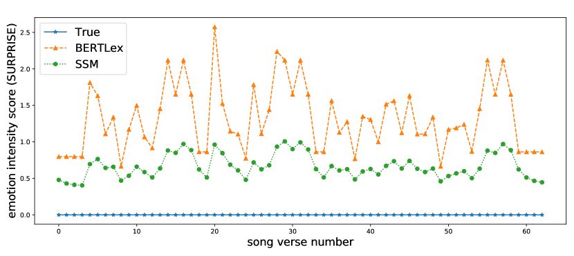
Figure 3: The SURPRISE emotion intensities of ground truth (all zeros), BERTLex model and SSM in an example song.

Characteristics of Kalman Filter and Kalman Smoother.

Our experiments indicate that initial predictions of at least 50 to 70 of 100 songs have been enhanced after modelling them with LG-SSMs. We summarize two trending types from the emotional dynamics of the songs whose predictions are weakened by LG-SSMs. One is that the gold-standard emotional dynamics fluctuate more sharply than those of the verse-level predictions, as displayed in the first and the second sub-figures in Figure 4. The other is the opposite that verse-level models produce an emotion intensity curve with more sudden changes than the gold-standard emotional dynamics (see the third sub-figure in Figure 4). The emotional dynamics trend of estimates by song-level models is similar to verse-level models. Due to the Gaussian assumption, Kalman Filter and Kalman Smoother tend to flatten or smooth the curves of verse-level predictions. This means that applying LG-SSMs can somewhat reduce errors in the second type of emotion dynamic curves. For the first type, however, the Kalman Filter and Kalman Smoother make the results worse, as smoother estimations are not desirable in this situation.

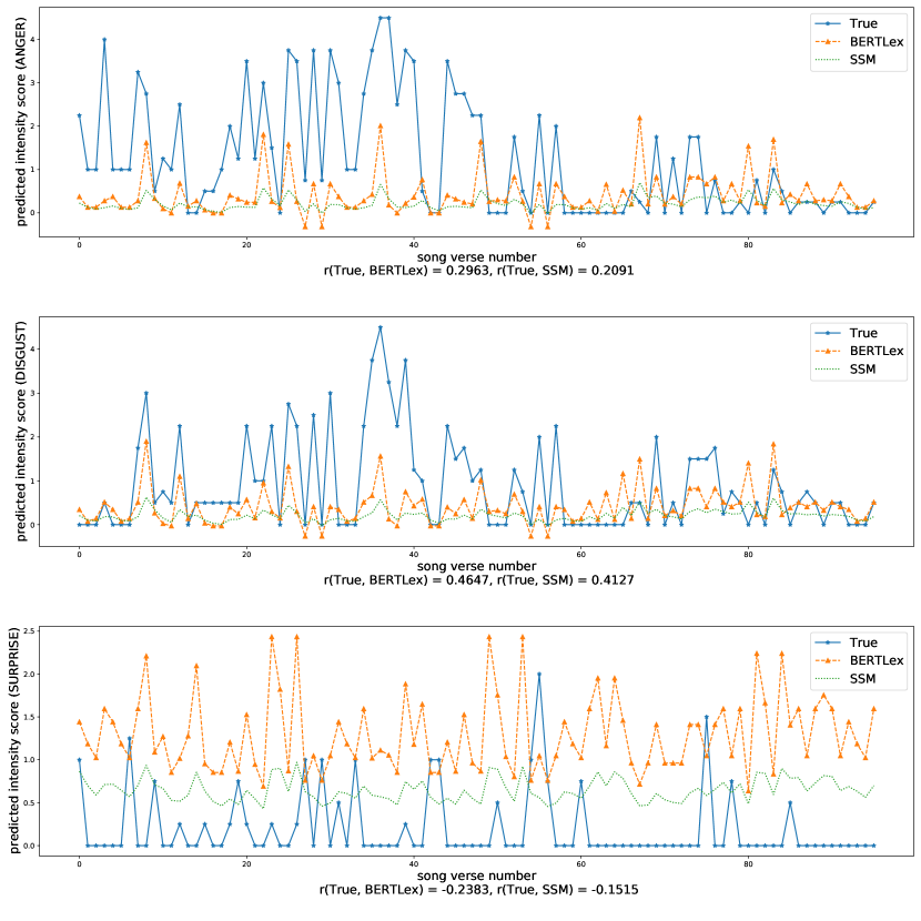
Figure 4: Emotional dynamics of ANGER, DISGUST and SURPRISE in Bad Romance by Lady Gaga: Pearson’s $r$ between ground truth and predictions of BERTLex^poly, estimates of Kalman Filter, are reported, respectively.

Using text solely.

Lyrics in LyricsEmotions are synchronised to acoustic features, where some verses with identical text are labelled as different emotional intensities. For instance, in Table 6, the verse "When it rain and rain, it rain and rain" repeats multiple times in the song Rain by Mika, and their gold-standard SADNESS labels differ in different verses as the emotion progresses with music. However, the verse-level models can only produce the same predictions since these verses share exactly the same text, and the models do not consider the context of the whole song. Consequently, the emotion scores of different verses predicted by LG-SSMs are close, as the results of song-level models are highly related to the initial predictions from BERTLex.

Verse ID	Gold	BERTLex	Smoother-EM
s55v15	4.33	8.65	1.68
s55v31	7.66	8.65	1.68
s55v32	7.33	8.65	1.63

Table 6: SADNESS scores of verses with the same lyrics verse "When it rain and rain, it rain and rain" but different gold-standard labels in the song.

6 Conclusion and Future Work

This paper presents a two-stage BERTLex-SSM framework for the sequence-labelling emotion intensity recognition tasks. Combining the contextualized embeddings with static word embeddings and then modelling the initial predicted intensity scores as a State Space model, our method can utilize context-sensitive features with external knowledge and capture the emotional dynamic transitions. Experimental results show that our proposed BERTLex-SSM effectively predicts emotion intensities in the lyrics without requiring annotated lyrics data.

Our analysis in Section 5.3 points to a range of directions for future work:

• While our method could apply any general verse-level model, including a pure lexicon-based one, in practice, we obtained the best results by leveraging annotated sentence-level datasets. This naturally leads to the domain discrepancy: in our particular case, between the news and lyrics domains. Given that unlabelled song lyrics are relatively easy to obtain, one direction is to incorporate unsupervised domain adaptation techniques (Ramponi and Plank, 2020) to improve the performance of the verse-level model. Semi-supervised learning (similar to Täckström and McDonald (2011b)) is another promising direction in this avenue, although methods would need to be modified to incorporate the continuous nature of the emotion labels.

• Despite being able to optimize the estimates through Kalman Filter and Kalman Smoother, the simplicity of the LG-SSM makes it difficult to deal with the wide variations in emotion space dynamics, given that it is a linear model. We hypothesize that non-linear SSM extensions (Julier and Uhlmann, 1997; Ito and Xiong, 2000; Julier and Uhlmann, 2004) might be a better fit for modelling emotion dynamics.

• As the LyricsEmotions dataset is annotated on parallel acoustic and text features, using lyrics solely as the feature can cause inconsistencies in the model. Extending our method to a multi-modal setting would remedy this issue when the identical lyrics are companions with different musical features to appear in various verses. Taking the knowledge of song structure (e.g., Intro - Verse - Bridge - Chorus) into account has the potential to advance the recognition of emotion dynamics, assuming the way (up or down) that emotion intensities change is correlated with which part of the song the verses locate.

References

- Agrawal et al. (2021) Yudhik Agrawal, Ramaguru Guru Ravi Shanker, and Vinoo Alluri. 2021. Transformer-based approach towards music emotion recognition from lyrics. In Advances in Information Retrieval, 43rd European Conference on IR Research (ECIR 2021), pages 167–175, Cham, Switzerland. Springer.
- Alghanmi et al. (2020) Israa Alghanmi, Luis Espinosa Anke, and Steven Schockaert. 2020. Combining BERT with static word embeddings for categorizing social media. In Proceedings of the Sixth Workshop on Noisy User-generated Text (W-NUT 2020), pages 28–33, Online. Association for Computational Linguistics.
- Besson et al. (1998) Mireille Besson, Frederique Faita, Isabelle Peretz, A-M Bonnel, and Jean Requin. 1998. Singing in the brain: Independence of lyrics and tunes. Psychological Science, 9(6):494–498.
- Brown et al. (2020) Tom Brown, Benjamin Mann, Nick Ryder, Melanie Subbiah, Jared D Kaplan, Prafulla Dhariwal, Arvind Neelakantan, Pranav Shyam, Girish Sastry, Amanda Askell, Sandhini Agarwal, Ariel Herbert-Voss, Gretchen Krueger, Tom Henighan, Rewon Child, Aditya Ramesh, Daniel Ziegler, Jeffrey Wu, Clemens Winter, Chris Hesse, Mark Chen, Eric Sigler, Mateusz Litwin, Scott Gray, Benjamin Chess, Jack Clark, Christopher Berner, Sam McCandlish, Alec Radford, Ilya Sutskever, and Dario Amodei. 2020. Language models are few-shot learners. In Advances in Neural Information Processing Systems, volume 33, pages 1877–1901. Curran Associates, Inc.
- Caetano et al. (2012) Marcelo Caetano, Athanasios Mouchtaris, and Frans Wiering. 2012. The role of time in music emotion recognition: Modeling musical emotions from time-varying music features. In International Symposium on Computer Music Modeling and Retrieval, pages 171–196. Springer.
- De Bruyne et al. (2021) Luna De Bruyne, Orphee De Clercq, and Veronique Hoste. 2021. Emotional RobBERT and insensitive BERTje: Combining transformers and affect lexica for Dutch emotion detection. In Proceedings of the Eleventh Workshop on Computational Approaches to Subjectivity, Sentiment and Social Media Analysis, pages 257–263, Online. Association for Computational Linguistics.
- Dempster et al. (1977) Arthur P Dempster, Nan M Laird, and Donald B Rubin. 1977. Maximum likelihood from incomplete data via the em algorithm. Journal of the Royal Statistical Society: Series B (Methodological), 39(1):1–22.
- Devlin et al. (2019) Jacob Devlin, Ming-Wei Chang, Kenton Lee, and Kristina Toutanova. 2019. BERT: Pre-training of deep bidirectional transformers for language understanding. In Proceedings of the 2019 Conference of the North American Chapter of the Association for Computational Linguistics: Human Language Technologies, Volume 1 (Long and Short Papers), pages 4171–4186, Minneapolis, Minnesota. Association for Computational Linguistics.
- Ekman (1993) Paul Ekman. 1993. Facial expression and emotion. American psychologist, 48(4):384.
- Esuli and Sebastiani (2007) Andrea Esuli and Fabrizio Sebastiani. 2007. Sentiwordnet: a high-coverage lexical resource for opinion mining. Evaluation, 17(1):26.
- Firdaus et al. (2020) Mauajama Firdaus, Hardik Chauhan, Asif Ekbal, and Pushpak Bhattacharyya. 2020. MEISD: A multimodal multi-label emotion, intensity and sentiment dialogue dataset for emotion recognition and sentiment analysis in conversations. In Proceedings of the 28th International Conference on Computational Linguistics, pages 4441–4453, Barcelona, Spain (Online). International Committee on Computational Linguistics.
- Ghosal et al. (2021) Deepanway Ghosal, Navonil Majumder, Rada Mihalcea, and Soujanya Poria. 2021. Exploring the role of context in utterance-level emotion, act and intent classification in conversations: An empirical study. In Findings of the Association for Computational Linguistics: ACL-IJCNLP 2021, pages 1435–1449, Online. Association for Computational Linguistics.
- Ghosal et al. (2019) Deepanway Ghosal, Navonil Majumder, Soujanya Poria, Niyati Chhaya, and Alexander Gelbukh. 2019. DialogueGCN: A graph convolutional neural network for emotion recognition in conversation. In Proceedings of the 2019 Conference on Empirical Methods in Natural Language Processing and the 9th International Joint Conference on Natural Language Processing (EMNLP-IJCNLP), pages 154–164, Hong Kong, China. Association for Computational Linguistics.
- Goel et al. (2017) Pranav Goel, Devang Kulshreshtha, Prayas Jain, and Kaushal Kumar Shukla. 2017. Prayas at EmoInt 2017: An ensemble of deep neural architectures for emotion intensity prediction in tweets. In Proceedings of the 8th Workshop on Computational Approaches to Subjectivity, Sentiment and Social Media Analysis, pages 58–65, Copenhagen, Denmark. Association for Computational Linguistics.
- Hazarika et al. (2018a) Devamanyu Hazarika, Soujanya Poria, Rada Mihalcea, Erik Cambria, and Roger Zimmermann. 2018a. ICON: Interactive conversational memory network for multimodal emotion detection. In Proceedings of the 2018 Conference on Empirical Methods in Natural Language Processing, pages 2594–2604, Brussels, Belgium. Association for Computational Linguistics.
- Hazarika et al. (2018b) Devamanyu Hazarika, Soujanya Poria, Amir Zadeh, Erik Cambria, Louis-Philippe Morency, and Roger Zimmermann. 2018b. Conversational memory network for emotion recognition in dyadic dialogue videos. In Proceedings of the 2018 Conference of the North American Chapter of the Association for Computational Linguistics: Human Language Technologies, Volume 1 (Long Papers), pages 2122–2132, New Orleans, Louisiana. Association for Computational Linguistics.
- Hsu et al. (2018) Chao-Chun Hsu, Sheng-Yeh Chen, Chuan-Chun Kuo, Ting-Hao Huang, and Lun-Wei Ku. 2018. EmotionLines: An emotion corpus of multi-party conversations. In Proceedings of the Eleventh International Conference on Language Resources and Evaluation (LREC 2018), Miyazaki, Japan. European Language Resources Association (ELRA).
- Hu et al. (2021) Dou Hu, Lingwei Wei, and Xiaoyong Huai. 2021. DialogueCRN: Contextual reasoning networks for emotion recognition in conversations. In Proceedings of the 59th Annual Meeting of the Association for Computational Linguistics and the 11th International Joint Conference on Natural Language Processing (Volume 1: Long Papers), pages 7042–7052, Online. Association for Computational Linguistics.
- Ishiwatari et al. (2020) Taichi Ishiwatari, Yuki Yasuda, Taro Miyazaki, and Jun Goto. 2020. Relation-aware graph attention networks with relational position encodings for emotion recognition in conversations. In Proceedings of the 2020 Conference on Empirical Methods in Natural Language Processing (EMNLP), pages 7360–7370, Online. Association for Computational Linguistics.
- Ito and Xiong (2000) Kazufumi Ito and Kaiqi Xiong. 2000. Gaussian filters for nonlinear filtering problems. IEEE transactions on automatic control, 45(5):910–927.
- Jiao et al. (2020) Wenxiang Jiao, Michael Lyu, and Irwin King. 2020. Real-time emotion recognition via attention gated hierarchical memory network. In Proceedings of the AAAI Conference on Artificial Intelligence, 05, pages 8002–8009.
- Julier and Uhlmann (1997) Simon J Julier and Jeffrey K Uhlmann. 1997. New extension of the kalman filter to nonlinear systems. In Signal processing, sensor fusion, and target recognition VI, volume 3068, pages 182–193. International Society for Optics and Photonics.
- Julier and Uhlmann (2004) Simon J Julier and Jeffrey K Uhlmann. 2004. Unscented filtering and nonlinear estimation. Proceedings of the IEEE, 92(3):401–422.
- Juslin and Laukka (2004) Patrik N Juslin and Petri Laukka. 2004. Expression, perception, and induction of musical emotions: A review and a questionnaire study of everyday listening. Journal of new music research, 33(3):217–238.
- Kalman (1960) Rudolph Emil Kalman. 1960. A new approach to linear filtering and prediction problems. Journal of Basic Engineering, 82(1):35–45.
- Kim et al. (2015) Seungyeon Kim, Joonseok Lee, Guy Lebanon, and Haesun Park. 2015. Estimating temporal dynamics of human emotions. In Proceedings of the Twenty-Ninth AAAI Conference on Artificial Intelligence, January 25-30, 2015, Austin, Texas, USA, pages 168–174. AAAI Press.
- Kim (2014) Yoon Kim. 2014. Convolutional neural networks for sentence classification. In Proceedings of the 2014 Conference on Empirical Methods in Natural Language Processing (EMNLP), pages 1746–1751, Doha, Qatar. Association for Computational Linguistics.
- Kim et al. (2010) Youngmoo E Kim, Erik M Schmidt, Raymond Migneco, Brandon G Morton, Patrick Richardson, Jeffrey Scott, Jacquelin A Speck, and Douglas Turnbull. 2010. Music emotion recognition: A state of the art review. In 11th International Society for Music Information Retrieval Conference (ISMIR 2010), volume 86, pages 255–266.
- Kipf and Welling (2017) Thomas N. Kipf and Max Welling. 2017. Semi-supervised classification with graph convolutional networks. In 5th International Conference on Learning Representations, ICLR 2017, Toulon, France, April 24-26, 2017, Conference Track Proceedings.
- Kiritchenko et al. (2014) Svetlana Kiritchenko, Xiaodan Zhu, and Saif M Mohammad. 2014. Sentiment analysis of short informal texts. Journal of Artificial Intelligence Research, 50:723–762.
- Koufakou et al. (2020) Anna Koufakou, Endang Wahyu Pamungkas, Valerio Basile, and Viviana Patti. 2020. HurtBERT: Incorporating lexical features with BERT for the detection of abusive language. In Proceedings of the Fourth Workshop on Online Abuse and Harms, pages 34–43, Online. Association for Computational Linguistics.
- Lafferty et al. (2001) John D. Lafferty, Andrew McCallum, and Fernando C. N. Pereira. 2001. Conditional random fields: Probabilistic models for segmenting and labeling sequence data. In Proceedings of the Eighteenth International Conference on Machine Learning (ICML 2001), Williams College, Williamstown, MA, USA, June 28 - July 1, 2001, pages 282–289. Morgan Kaufmann.
- Li et al. (2020) Jingye Li, Donghong Ji, Fei Li, Meishan Zhang, and Yijiang Liu. 2020. HiTrans: A transformer-based context- and speaker-sensitive model for emotion detection in conversations. In Proceedings of the 28th International Conference on Computational Linguistics, pages 4190–4200, Barcelona, Spain (Online). International Committee on Computational Linguistics.
- Li et al. (2017) Yanran Li, Hui Su, Xiaoyu Shen, Wenjie Li, Ziqiang Cao, and Shuzi Niu. 2017. DailyDialog: A manually labelled multi-turn dialogue dataset. In Proceedings of the Eighth International Joint Conference on Natural Language Processing (Volume 1: Long Papers), pages 986–995, Taipei, Taiwan. Asian Federation of Natural Language Processing.
- Lian et al. (2020) Zheng Lian, Jianhua Tao, Bin Liu, Jian Huang, Zhanlei Yang, and Rongjun Li. 2020. Conversational emotion recognition using self-attention mechanisms and graph neural networks. In Interspeech 2020, 21st Annual Conference of the International Speech Communication Association, Virtual Event, Shanghai, China, 25-29 October 2020, pages 2347–2351. ISCA.
- Lu et al. (2020) Xin Lu, Yanyan Zhao, Yang Wu, Yijian Tian, Huipeng Chen, and Bing Qin. 2020. An iterative emotion interaction network for emotion recognition in conversations. In Proceedings of the 28th International Conference on Computational Linguistics, pages 4078–4088, Barcelona, Spain (Online). International Committee on Computational Linguistics.
- Majumder et al. (2019) Navonil Majumder, Soujanya Poria, Devamanyu Hazarika, Rada Mihalcea, Alexander Gelbukh, and Erik Cambria. 2019. Dialoguernn: An attentive rnn for emotion detection in conversations. In Proceedings of the AAAI Conference on Artificial Intelligence, volume 33, pages 6818–6825.
- Malheiro et al. (2016) Ricardo Malheiro, Renato Panda, Paulo Gomes, and Rui Pedro Paiva. 2016. Emotionally-relevant features for classification and regression of music lyrics. IEEE Transactions on Affective Computing, 9(2):240–254.
- McCallum et al. (2000) Andrew McCallum, Dayne Freitag, and Fernando C. N. Pereira. 2000. Maximum entropy markov models for information extraction and segmentation. In Proceedings of the Seventeenth International Conference on Machine Learning (ICML 2000), Stanford University, Stanford, CA, USA, June 29 - July 2, 2000, pages 591–598. Morgan Kaufmann.
- McDonald et al. (2007) Ryan McDonald, Kerry Hannan, Tyler Neylon, Mike Wells, and Jeff Reynar. 2007. Structured models for fine-to-coarse sentiment analysis. In Proceedings of the 45th Annual Meeting of the Association of Computational Linguistics, pages 432–439, Prague, Czech Republic. Association for Computational Linguistics.
- McKeown et al. (2011) Gary McKeown, Michel Valstar, Roddy Cowie, Maja Pantic, and Marc Schroder. 2011. The semaine database: Annotated multimodal records of emotionally colored conversations between a person and a limited agent. IEEE transactions on affective computing, 3(1):5–17.
- Mehta et al. (2020) Yash Mehta, Samin Fatehi, Amirmohammad Kazameini, Clemens Stachl, Erik Cambria, and Sauleh Eetemadi. 2020. Bottom-up and top-down: Predicting personality with psycholinguistic and language model features. In 2020 IEEE International Conference on Data Mining (ICDM), pages 1184–1189. IEEE.
- Meisheri and Dey (2018) Hardik Meisheri and Lipika Dey. 2018. TCS research at SemEval-2018 task 1: Learning robust representations using multi-attention architecture. In Proceedings of The 12th International Workshop on Semantic Evaluation, pages 291–299, New Orleans, Louisiana. Association for Computational Linguistics.
- Mihalcea and Strapparava (2012) Rada Mihalcea and Carlo Strapparava. 2012. Lyrics, music, and emotions. In Proceedings of the 2012 Joint Conference on Empirical Methods in Natural Language Processing and Computational Natural Language Learning, pages 590–599.
- Mohammad (2018) Saif Mohammad. 2018. Word affect intensities. In Proceedings of the Eleventh International Conference on Language Resources and Evaluation (LREC 2018), Miyazaki, Japan. European Language Resources Association (ELRA).
- Mohammad et al. (2018a) Saif Mohammad, Felipe Bravo-Marquez, Mohammad Salameh, and Svetlana Kiritchenko. 2018a. SemEval-2018 task 1: Affect in tweets. In Proceedings of The 12th International Workshop on Semantic Evaluation, pages 1–17, New Orleans, Louisiana. Association for Computational Linguistics.
- Mohammad et al. (2018b) Saif Mohammad, Felipe Bravo-Marquez, Mohammad Salameh, and Svetlana Kiritchenko. 2018b. SemEval-2018 task 1: Affect in tweets. In Proceedings of The 12th International Workshop on Semantic Evaluation, pages 1–17, New Orleans, Louisiana. Association for Computational Linguistics.
- Mohammad et al. (2013) Saif Mohammad, Svetlana Kiritchenko, and Xiaodan Zhu. 2013. Nrc-canada: Building the state-of-the-art in sentiment analysis of tweets. In Second Joint Conference on Lexical and Computational Semantics (* SEM), Volume 2: Proceedings of the Seventh International Workshop on Semantic Evaluation (SemEval 2013), pages 321–327.
- Mohammad and Bravo-Márquez (2017) Saif M Mohammad and Felipe Bravo-Márquez. 2017. Wassa-2017 shared task on emotion intensity. In 8th Workshop on Computational Approaches to Subjectivity, Sentiment and Social Media Analysis WASSA 2017: Proceedings of the Workshop, pages 34–49. The Association for Computational Linguistics.
- Mohammad and Kiritchenko (2015) Saif M Mohammad and Svetlana Kiritchenko. 2015. Using hashtags to capture fine emotion categories from tweets. Computational Intelligence, 31(2):301–326.
- Mohammad and Turney (2013) Saif M Mohammad and Peter D Turney. 2013. Crowdsourcing a word–emotion association lexicon. Computational Intelligence, 29(3):436–465.
- Murphy (2012) Kevin P. Murphy. 2012. Machine learning: a probabilistic perspective. MIT press.
- Nair and Hinton (2010) Vinod Nair and Geoffrey E Hinton. 2010. Rectified linear units improve restricted boltzmann machines. In Proceedings of the 27th International Conference on International Conference on Machine Learning, pages 807–814.
- Nozza et al. (2017) Debora Nozza, Elisabetta Fersini, and Enza Messina. 2017. A multi-view sentiment corpus. In Proceedings of the 15th Conference of the European Chapter of the Association for Computational Linguistics: Volume 1, Long Papers, pages 273–280, Valencia, Spain. Association for Computational Linguistics.
- Plutchik (1980) Robert Plutchik. 1980. A general psychoevolutionary theory of emotion. In Theories of emotion, pages 3–33. Elsevier.
- Poria et al. (2017) Soujanya Poria, Erik Cambria, Devamanyu Hazarika, Navonil Majumder, Amir Zadeh, and Louis-Philippe Morency. 2017. Context-dependent sentiment analysis in user-generated videos. In Proceedings of the 55th Annual Meeting of the Association for Computational Linguistics (Volume 1: Long Papers), pages 873–883, Vancouver, Canada. Association for Computational Linguistics.
- Poria et al. (2019a) Soujanya Poria, Devamanyu Hazarika, Navonil Majumder, Gautam Naik, Erik Cambria, and Rada Mihalcea. 2019a. MELD: A multimodal multi-party dataset for emotion recognition in conversations. In Proceedings of the 57th Annual Meeting of the Association for Computational Linguistics, pages 527–536, Florence, Italy. Association for Computational Linguistics.
- Poria et al. (2019b) Soujanya Poria, Navonil Majumder, Rada Mihalcea, and Eduard Hovy. 2019b. Emotion recognition in conversation: Research challenges, datasets, and recent advances. IEEE Access, 7:100943–100953.
- Rabiner and Juang (1986) Lawrence Rabiner and Biinghwang Juang. 1986. An introduction to hidden markov models. IEEE ASSP Magazine, 3(1):4–16.
- Ramachandran and de Melo (2020) Arun Ramachandran and Gerard de Melo. 2020. Cross-lingual emotion lexicon induction using representation alignment in low-resource settings. In Proceedings of the 28th International Conference on Computational Linguistics, pages 5879–5890, Barcelona, Spain (Online). International Committee on Computational Linguistics.
- Ramponi and Plank (2020) Alan Ramponi and Barbara Plank. 2020. Neural unsupervised domain adaptation in NLP—A survey. In Proceedings of the 28th International Conference on Computational Linguistics, pages 6838–6855, Barcelona, Spain (Online). International Committee on Computational Linguistics.
- Rauch et al. (1965) Herbert E Rauch, F Tung, and Charlotte T Striebel. 1965. Maximum likelihood estimates of linear dynamic systems. AIAA journal, 3(8):1445–1450.
- Rogers et al. (2021) Anna Rogers, Olga Kovaleva, and Anna Rumshisky. 2021. A Primer in BERTology: What We Know About How BERT Works. Transactions of the Association for Computational Linguistics, 8:842–866.
- Russell (1980) James A Russell. 1980. A circumplex model of affect. Journal of personality and social psychology, 39(6):1161–1178.
- Schmidt and Kim (2010) Erik M Schmidt and Youngmoo E Kim. 2010. Prediction of time-varying musical mood distributions using kalman filtering. In 2010 Ninth International Conference on Machine Learning and Applications, pages 655–660. IEEE.
- Schmidt and Kim (2011) Erik M Schmidt and Youngmoo E Kim. 2011. Modeling musical emotion dynamics with conditional random fields. In Proceedings of the 12th International Society for Music Information Retrieval Conference, ISMIR, pages 777–782. Miami (Florida), USA.
- Schmidt et al. (2010) Erik M Schmidt, Douglas Turnbull, and Youngmoo E Kim. 2010. Feature selection for content-based, time-varying musical emotion regression. In Proceedings of the 11th ACM SIGMM International Conference on Multimedia Information Retrieval, pages 267–274.
- Shen et al. (2021) Weizhou Shen, Siyue Wu, Yunyi Yang, and Xiaojun Quan. 2021. Directed acyclic graph network for conversational emotion recognition. In Proceedings of the 59th Annual Meeting of the Association for Computational Linguistics and the 11th International Joint Conference on Natural Language Processing (Volume 1: Long Papers), pages 1551–1560, Online. Association for Computational Linguistics.
- Srivastava et al. (2014) Nitish Srivastava, Geoffrey E. Hinton, Alex Krizhevsky, Ilya Sutskever, and Ruslan Salakhutdinov. 2014. Dropout: a simple way to prevent neural networks from overfitting. The Journal of Machine Learning Research, 15(1):1929–1958.
- Staiano and Guerini (2014) Jacopo Staiano and Marco Guerini. 2014. Depeche mood: a lexicon for emotion analysis from crowd annotated news. In Proceedings of the 52nd Annual Meeting of the Association for Computational Linguistics (Volume 2: Short Papers), pages 427–433, Baltimore, Maryland. Association for Computational Linguistics.
- Strapparava and Mihalcea (2007) Carlo Strapparava and Rada Mihalcea. 2007. SemEval-2007 task 14: Affective text. In Proceedings of the Fourth International Workshop on Semantic Evaluations (SemEval-2007), pages 70–74, Prague, Czech Republic. Association for Computational Linguistics.
- Täckström and McDonald (2011a) Oscar Täckström and Ryan McDonald. 2011a. Discovering fine-grained sentiment with latent variable structured prediction models. In European Conference on Information Retrieval, pages 368–374. Springer.
- Täckström and McDonald (2011b) Oscar Täckström and Ryan McDonald. 2011b. Semi-supervised latent variable models for sentence-level sentiment analysis. In Proceedings of the 49th Annual Meeting of the Association for Computational Linguistics: Human Language Technologies, pages 569–574, Portland, Oregon, USA. Association for Computational Linguistics.
- Williams (1959) Evan J Williams. 1959. The comparison of regression variables. Journal of the Royal Statistical Society: Series B (Methodological), 21(2):396–399.
- Wu et al. (2014) Bin Wu, Erheng Zhong, Andrew Horner, and Qiang Yang. 2014. Music emotion recognition by multi-label multi-layer multi-instance multi-view learning. In Proceedings of the 22nd ACM International Conference on Multimedia, pages 117–126.
- Wu et al. (2016) Yonghui Wu, Mike Schuster, Zhifeng Chen, Quoc V. Le, Mohammad Norouzi, Wolfgang Macherey, Maxim Krikun, Yuan Cao, Qin Gao, Klaus Macherey, Jeff Klingner, Apurva Shah, Melvin Johnson, Xiaobing Liu, Lukasz Kaiser, Stephan Gouws, Yoshikiyo Kato, Taku Kudo, Hideto Kazawa, Keith Stevens, George Kurian, Nishant Patil, Wei Wang, Cliff Young, Jason Smith, Jason Riesa, Alex Rudnick, Oriol Vinyals, Greg Corrado, Macduff Hughes, and Jeffrey Dean. 2016. Google’s neural machine translation system: Bridging the gap between human and machine translation. CoRR, abs/1609.08144.
- Yang et al. (2019) Zhilin Yang, Zihang Dai, Yiming Yang, Jaime Carbonell, Russ R Salakhutdinov, and Quoc V Le. 2019. Xlnet: Generalized autoregressive pretraining for language understanding. In Advances in Neural Information Processing Systems, volume 32. Curran Associates, Inc.
- Ying et al. (2019) Wenhao Ying, Rong Xiang, and Qin Lu. 2019. Improving multi-label emotion classification by integrating both general and domain-specific knowledge. In Proceedings of the 5th Workshop on Noisy User-generated Text (W-NUT 2019), pages 316–321, Hong Kong, China. Association for Computational Linguistics.
- Zhang et al. (2019) Dong Zhang, Liangqing Wu, Changlong Sun, Shoushan Li, Qiaoming Zhu, and Guodong Zhou. 2019. Modeling both context- and speaker-sensitive dependence for emotion detection in multi-speaker conversations. In Proceedings of the Twenty-Eighth International Joint Conference on Artificial Intelligence, IJCAI 2019, Macao, China, August 10-16, 2019, pages 5415–5421. ijcai.org.
- Zhang et al. (2020) Zhuosheng Zhang, Yuwei Wu, Hai Zhao, Zuchao Li, Shuailiang Zhang, Xi Zhou, and Xiang Zhou. 2020. Semantics-aware bert for language understanding. In Proceedings of the AAAI Conference on Artificial Intelligence, volume 34, pages 9628–9635.
- Zhao et al. (2022) Weixiang Zhao, Yanyan Zhao, and Xin Lu. 2022. Cauain: Causal aware interaction network for emotion recognition in conversations. In Proceedings of the Thirty-First International Joint Conference on Artificial Intelligence, IJCAI 2022, Vienna, Austria, 23-29 July 2022, pages 4524–4530. ijcai.org.
- Zhong et al. (2019) Peixiang Zhong, Di Wang, and Chunyan Miao. 2019. Knowledge-enriched transformer for emotion detection in textual conversations. In Proceedings of the 2019 Conference on Empirical Methods in Natural Language Processing and the 9th International Joint Conference on Natural Language Processing (EMNLP-IJCNLP), pages 165–176, Hong Kong, China. Association for Computational Linguistics.
- Zhou et al. (2020) Deyu Zhou, Shuangzhi Wu, Qing Wang, Jun Xie, Zhaopeng Tu, and Mu Li. 2020. Emotion classification by jointly learning to lexiconize and classify. In Proceedings of the 28th International Conference on Computational Linguistics, COLING 2020, Barcelona, Spain (Online), December 8-13, 2020, pages 3235–3245. International Committee on Computational Linguistics.
- Zhu et al. (2014) Xiaodan Zhu, Svetlana Kiritchenko, and Saif Mohammad. 2014. NRC-Canada-2014: Recent improvements in the sentiment analysis of tweets. In Proceedings of the 8th International Workshop on Semantic Evaluation (SemEval 2014), pages 443–447, Dublin, Ireland. Association for Computational Linguistics.