COMET SCIENCE WITH GROUND BASED AND SPACE BASED SURVEYS IN THE NEW MILLENNIUM

Abstract

• We summarize the comet science provided by surveys. This includes surveys where the detections of comets are an advantageous benefit but were not part of the survey’s original intent, as well as some pointed surveys where comet science was the goal. Many of the surveys are made using astrophysical and heliophysics assets. The surveys in our scope include those using ground-based as well as space-based telescope facilities. Emphasis is placed on current or recent surveys, and science that has resulted since the publication of Comets II, though key advancements made by earlier surveys (e.g. IRAS, COBE, NEAT, etc.) will be mentioned. The proportionally greater number of discoveries of comets by surveys have yielded in turn larger samples of comet populations and sub-populations for study, resulting in better defined evolutionary trends. While providing an array of remarkable discoveries, most of the survey data has been only cursorily investigated. It is clear that continuing to fund ground- and space-based surveys of large numbers of comets is vital if we are to address science goals that can give us a population-wide picture of comet properties.
   
   
  

1 INTRODUCTION

Over the span of the last decade and a half, a more automated approach to the analysis of data has become common. This is in part owing to the arrival of data sets which are so large that each of the observations is not practically analyzed by human interaction, but rather is conducted by automated pipeline. Analysis routines are prototyped, tested, and applied to larger datasets, while outliers and diagnostic triggers indicate where special circumstances apply, and further manipulation, or rejection, of the data are required. Much of this has been driven by the advent of the vast quantities of data provided by automated sky surveys. Additionally specialized data sets that are the product of targeted observations now have a certain expectation of providing statistically significant samples large enough for outliers to be identified and trends to be discerned.

Previous generation surveys generally had relatively small sample sizes. Many of these surveys, demonstrably the space-based surveys, made robust discoveries with these smaller samples. Lisse et al. (1998) found temperature excess in dust comae from observations of five comets at perihelion distances $\sim 1$au obtained by the Cosmic Microwave Background Explorer (COBE). Röntgen Satellite (ROSAT) observations of six (Dennerl et al., 1997), and later eleven (c.f. Lisse et al. 2004), comets revealed charge exchange between highly charged heavy ions in the solar wind and cometary neutrals dominated cometary X-ray emissions. A subsequent survey by Bodewits et al. (2007) of eight comets with the Chandra observatory found that the characteristics of observed X-ray spectra mainly reflect the state of the local solar wind. The Infrared Astronomy Satellite (IRAS) mission data provided the first thermal dust trail measurements from eight identified comets (Sykes and Walker, 1992). Such surveys had large impacts on the cometary field, but did not employ the more automated large-sample approaches, such as with astroinformatic techniques (c.f. Borne et al. 2009), now utilized for larger survey samples.

For the definition of survey within these pages, we include sample sizes of 20 or greater, owing to the conditions that even for simple statistical correlation tests, sample sizes $\sim 20$ or greater are required to achieve $95\%$ confidence values even for strong correlations (c.f. Bonnet and Wright 2000). Here we concentrate on classical comet populations (long-period and short-period comets; LPCs and SPCs, respectively) and their dynamically defined sub-classifications (c.f. Levison 1996). SPCs are defined to have orbital periods $<200$ years, and LPCs having orbit periods $\gtrsim 200$ years. Jupiter Family Comets (JFCs), for example, are a sub-class of SPCs with orbital periods $\lesssim 20$ years and pro-grade low orbital inclinations $\lesssim 40^{\circ}$, while dynamically new comets are a sub-class of LPCs with original orbital semi-major axis values $\gtrsim 10^{4}$ au. Generally speaking, the source of LPCs is the Oort cloud while the Kuiper belt feeds the population of SPCs. Notably Halley-type comets (HTCs) have historically often been lumped with SPCs, but most of them are likely to be highly-evolved (in the dynamics sense) objects from the Oort Cloud. Thus they are more closely related to the LPCs. There are also different opinions on the meaning of the term ’Oort Cloud comet’; e.g., it may only include dynamically new comets, or it may include all LPCs and HTCs that were in the Oort Cloud any time in the past.

Measurements of large populations from single platforms and the same, or similar, instrumentation provide a basis for comparative samples, in contrast with compilations (c.f. A’Hearn et al. 1995, Lisse et al. 2020 and A’Hearn et al. 2012). Such samples of cometary physical properties may be targeted, such as narrow-band filter surveys (cf. Schleicher and Farnham 2004) or spectroscopic surveys (cf. Dello Russo et al. 2016), or serendipitous observations, such as the data obtained with many ground-based or space-based sky surveys. These two categories are significantly different in the selection of the objects observed, and how representative the samples are of the background populations.

In the first case of targeted samples, known solar-system object targets are selected based on their optical brightness, and were discovered often by sky surveys. They are often observed at preferred geometries (opposition, for example, for ground based telescopic surveys) and detected while they are most active. As such, there are potential selection biases in the sample that may skew projection of behavior or physical properties of the base population. For targeted observations the observing time can be selected to sample the points through a comet’s orbit where the expected levels of activity are best matched to the physical property of interest. For example, optical surveys of comets at aphelion may provide more accurate absolute magnitude values of the nucleus, leading to better derived reflectances if the size of the body is known. Alternatively, a more comprehensive inventory of gas species may be derived at perihelion where so-called hyper-volatiles and water-related species are released, and following a comet through its orbit may reveal when particular species dominate the activity.

1.1 Survey Discoveries of Comets

Prior to the 1990s, comets were generally discovered either in large photographic plate exposures or by individuals that visually scanned the sky, often employing specialized telescopes or binoculars with fast optics. In the late 1980s and early 1990s, digital cameras began to be employed in regular searches of the sky for solar system objects (cf. Scotti et al. 1991) with a handful of early comet discoveries. In addition, astrophysical sky surveys were conceived to identify transient behavior, like supernova events, in extra-solar-system objects. With the advent of the earliest digital sky surveys, the automated surveys began to make significant contributions in the number of comet discoveries in the mid-1990s. These foundational surveys employed Charge-Coupled Device (CCD) cameras with fields of view that by today’s standards would be quite modest, on the order of a degree on a side (c.f. Pravdo et al. 1999), and rapidly began to outpace other means of discovery.

The efforts to detect solar system objects have been largely driven by the intent to discover and characterize Near Earth Objects (NEOs). Observing cadences, pointing strategy, and approaches to analysis were therefore optimized or prioritized towards these NEO-related goals. These efforts have been remarkably effective, and discovery of more than 83% of the known NEOs has been the result of these efforts (Landis and Johnson, 2019). As a means of discovering comets, the NEO search programs have also been effective, not only with the comets that are a component of the NEO population, but also with more distant comets.

As of September 30, 2021, approximately 3586 comets had been discovered, as registered by the Jet Propulsion Laboratory (JPL) small bodies database. A summary of leading discovery platforms is provided in Table 1. According to the database, 41$\%$ of the comet discoveries listed were discovered by the Solar and Heliospheric Observatory (SOHO; with the SWAN and LASCO instruments) or the Solar Terrestrial Relations Observatory (STEREO) spacecraft. In total, including these surveys, over 71% of comet discoveries up to October 2021 have been made by sky surveys. It is worth noting that the Minor Planet Center count ($\sim$4430 comets as of September 30, 2021), and future counts in the near term, are likely to be higher, as a significant remainder of the data from the SOHO spacecraft have yet to be processed and the JPL number includes only those comets that have been observed by other non-solar-observing platforms in addition. Figure 1 shows the annual number of discoveries and observations of objects by sky surveys reported to the MPC and listed in the JPL database. The drop-off in the discoveries near 2010 coincides with the curtailment of sun-pointing spacecraft survey data by the MPC, which has been recently resumed (Battams and Boonplod, 2020), though has not yet encompassed the multi-year backlog (Battams and Knight, 2017).

Table 1: Comet Discoveries by Selected Sky Surveys

Survey	Locationa	SPCsb	LPCsb	Total
Catalina	G96, 703, I52	200	193	393
Pan-STARRS	F51, F52	112	142	254
LINEAR	704	91	128	219
NEAT	566, 644	39	16	55
ATLAS	T05, T07, T08	16	35	51
NEOWISE	C51	16	23	39
Spacewatch	291, 691	16	12	28
LONEOS	699	17	5	22
ZTF/PTF	I41	2	16	18
SOHO/SWANc	249	12	1466	1478
STEREOc	C49	1	8	9

aThe Minor Planet Center Observatory Code contributors. bShort-period comets (SPCs) with orbital periods $<200$ years
and Long-period comets (LPCs) with orbital periods $\geq 200$ years. cSun-looking survey total. Note that the count of SOHO-discovered comets include
only those contributions with additional non-SOHO observations (see text).

1.2 Survey Observations

Along with a marked increase in the number of comet discoveries brought through ground-based surveys, the number of observations of comets has increased as well. Figure 1 shows that the number of observations closely tracks the number of objects observed by the surveys. On average, an object is observed on the order of 10 times per year, during its range of detectability, e.g. while the comet passes through its perihelion. Table 2 lists the number of observations from each of the leading five surveys at 5 year intervals back to 2000. The table shows the number of comet observations is relatively small compared with the total observations of small bodies. It also reveals the slowly changing ranks (in order of total observations) in the lead surveys. The output of some very active programs are temporarily diminished (cf. NEAT in the year 2000); each program either upgrades and incorporates more sites, or becomes outpaced by competing surveys, in which case existing survey programs or sites often shift to a priority from discovery to highly productive follow-up.

Both ground-based and space-based sky surveys have been used to characterize cometary populations. However, the full and systematic utilization of the majority of data obtained by the surveys is in its early stages, with only a handful of instances of the data being used to quantitatively characterize the comet populations. Much of the initial exploration of these sky survey datasets are centered around characterization of particular comets of interest. Dobson et al. (2021) use Asteroid Terrestrial-impact Last Alert System (ATLAS) data to identify the longevity of 95P/Chiron’s 2018 onset of activity. Zwicky Transient Factory (ZTF) survey (Kelley et al., 2021), Transiting Exoplanet Survey Satellite (TESS) spacecraft (Farnham et al., 2019), and NEOWISE survey (Bauer et al., 2021) observations were used to monitor and characterize the behavior of 46P/Wirtanen during its 2019 perihelion approach. Investigations of statistically significant samples of comet populations (c.f. Farnham et al. 2021) are likewise facilitated by sky surveys, and are beginning to be analyzed using astroinformatic approaches. Larger surveys that compile cometary populations to constrain populations statistics are rarer still. Hicks et al. (2007) reported magnitudes and Af$\rho$ values (c.f. A’Hearn et al. 1984) for 52 comets observed by the Near Earth Asteroid Telescope (NEAT) between 2001 and 2003, and produced estimates of nucleus size for 25 of the lowest-activity comets in the sample. Searches for cometary activity among asteroids are more common (see also Jewitt et al. in this volume). Waszczak et al. (2013) searched for undiscovered main-belt comets, but identified 115 comets in the Palomar Transient Factory (PTF) data taken from 2009 through 2012, listing the maximum and minimum magnitudes observed in the images. Sonnett et al. (2011) observed 924 asteroids, and Hsieh et al. (2015) conducted a large search of main belt objects observed in Panoramic Survey Telescope and Rapid Response System (Pan-STARRS) data to find cometary activity, while Martino et al. (2019) and Mommert et al. (2020) searched for activity amongst asteroids in comet-like orbits.

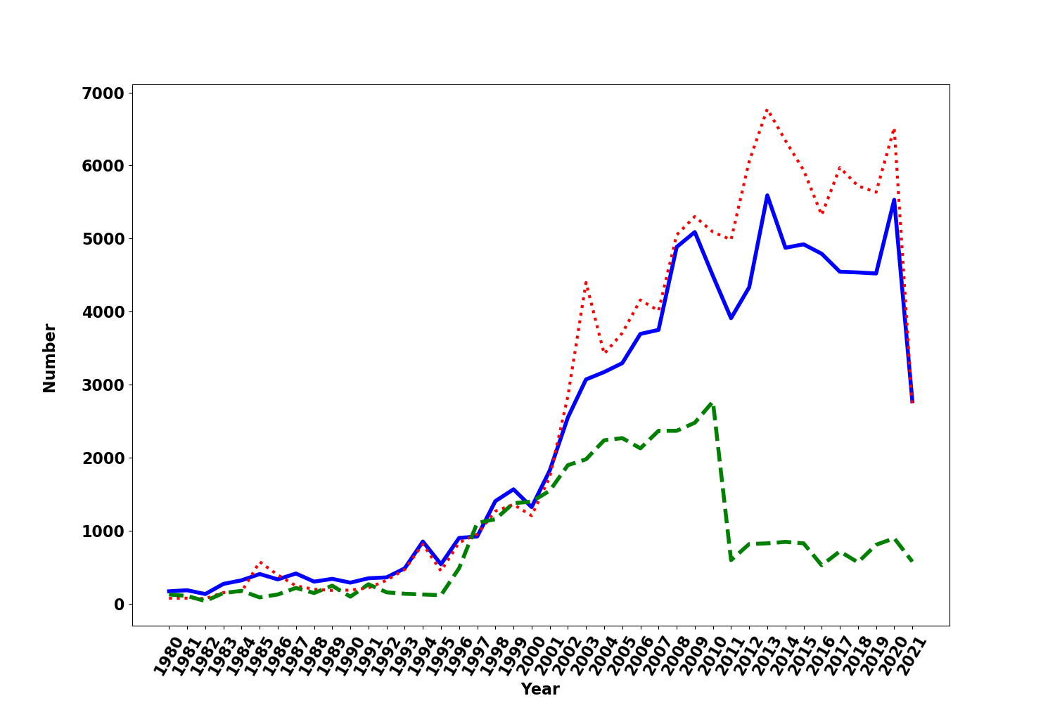
Figure 1: Discoveries and reported observations of comets per year, 1980-2021. Green dashed line indicates discoveries per year (multiplied by 10) as listed in the JPL small bodies database (but see text for explanation of the 2010 drop off). Blue solid line indicates the number of comets with observations reported to the MPC. Red dotted line indicates the number of observations reported to the MPC (divided by 10).

1.3 Survey Biases

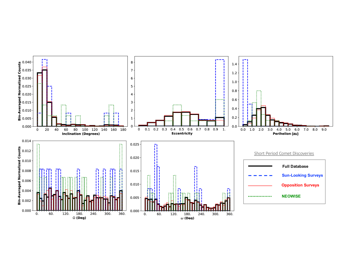
Figure 2: The relative distributions of the orbital elements of short period comet (SPC) discoveries from the JPL small bodies database are shown. The database’s SPC populations are shown in total (black histogram), and compared with representative samples of contributions from sun-looking surveys (blue dashed line; SOHO, SWAN, and STEREO comets), opposition pointing surveys (red thin solid line) and terminator pointing (green dotted line; NEOWISE) surveys. Scaled distribution histograms are shown for orbital inclination (upper left), eccentricity (upper middle), perihelion (upper right), ascending node (lower left) and argument of perihelion (middle left). Note that each histogram is plotted with bin-averaged, normalized counts, such that the sum of the counts times the bin-width across all the bins equal 1.

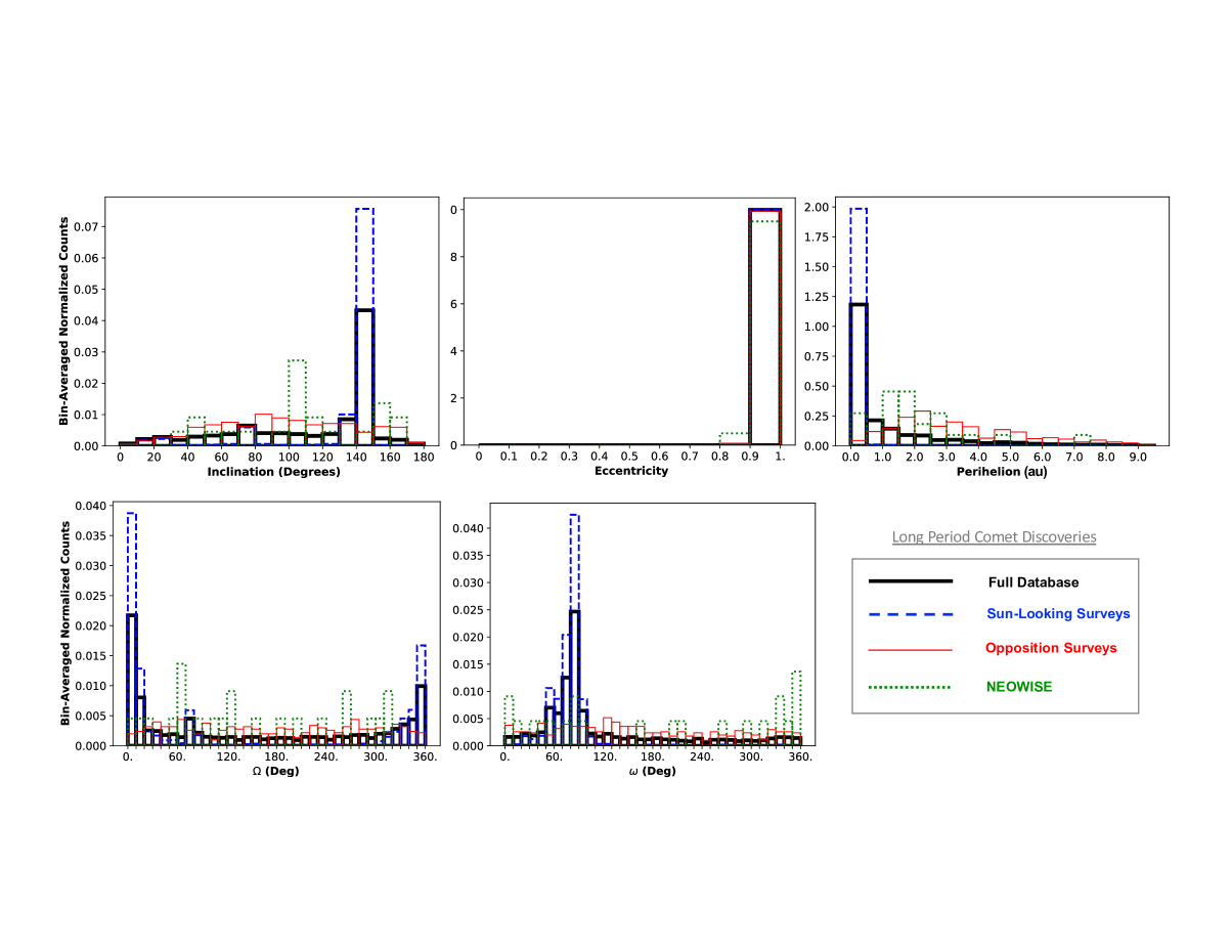
Figure 3: Similar to Fig. 2, the relative distribution of the orbital elements, here for the long period comet (LPC) discoveries from the JPL small bodies database are shown. The database’s LPC populations are shown in total (black histogram), and compared with representative samples of contributions from sun-looking surveys (blue dashed line; SOHO, SWAN, and STEREO comets), opposition pointing surveys (red thin solid line) and terminator pointing (green dotted line; NEOWISE) surveys. Scaled distribution histograms are shown for orbital inclination (upper left), eccentricity (upper middle), perihelion (upper right), ascending node (lower left) and argument of perihelion (middle left).

It is abundantly clear from the previous discussion that sky and sun-pointing surveys have had a remarkable impact on our statistical understanding of the comet populations. However, these data possess limitations, according to their sensitivities, coverage strategies, and cadences. Non-survey observations remain, therefore, highly valuable to the community, as demonstrated in the discovery of the second interstellar object (cf. Borisov and Shustov 2021). Figs 2 and 3 are illustrative of the sample biases that can remain even when short term biases, like those imposed by weather, are removed or averaged over, and how they can be convolved with real population features. The SPC inclination features are mostly real, and are dominated by the JFC population’s clustering near low-inclination orbits. The outliers in inclination, around near-retrograde orbits, have contributions from the active Centaur and Halley-type comet populations. Eccentricity is nearly level, but falls off at near zero values, corresponding to near-circular orbits; the high-eccentricity outliers on short-period orbits are in part strengthened by the near sun-grazing comets seen by sun-looking surveys (SLSs), or higher elongation, or terminator-pointing surveys (TPSs), like NEOWISE. Comets tend to be most active as they approach towards and retreat from their perihelion distance, so the discoveries with the furthest perihelia are made first by the opposition-looking surveys, while the TPSs make the near-earth perihelion discoveries, and the remaining low-perihelion comets are found by SLSs. The dips near 80 and 270 degrees in the SPC argument of perihelion ($\omega$) distributions roughly correspond to where the tug of Jupiter disrupts SPC orbits.

For the LPCs, in contrast to the SPCs, the discoveries are dominated by SLSs, and thus a few high-inclination sun-grazing comets, particularly the Kreutz family comets. The NEOWISE weak cluster in inclination, near 105^∘, pointed out in Bauer et al. (2017), has become mildly more pronounced with additional survey data, and the peaks in ascending node ($\Omega$) and $\omega$ are clustering from the noted Kreutz family comets. In each survey approach, the success with particular populations show statistical outliers that can bias the derived distributions if naively extrapolated from the observed distributions or not carefully removed.

The large representative samples of comets discovered and observed by sky surveys facilitates analyses of their total populations that lead to constraints on their total numbers. Such derivations are common among other representative populations, for example with NEOs (Mainzer et al., 2012) and Centaurs (Jedicke and Herron, 1997). Accurate accounting of factors that affect the survey’s detection efficiency, such as observing cadence, pointing pattern and viewing geometry, sensitivity, and weather (for ground-based surveys) are critical to the assessment of the underlying population numbers from the observations. Owing to these factors being intrinsic to each survey (or instrument/telescope combination), they must be considered for each separate contribution. Comets, however, are different from other populations in that they require an extra layer of accounting to derive the final total population numbers from the observed sample; the brightness variations from activity have to be accounted as well. Comets tend to vary greatly in their brightness throughout their orbit, usually achieving peak brightness around, though often not precisely at, their perihelion. Even surveys with more predictable observing circumstances, e.g. space-based surveys, have an additional significant level of uncertainty on any derived constraints of total populations.

Table 2: Yearly Comet Survey Observations^a

Surveyb	Totalc	Comets	Comet
	Detectionsd	Observed	Detectionsd
2020
Pan-STARRS	12181991	344	3606
ATLAS	10396137	284	11787
Catalina	10134103	335	4754
NEOWISE	152141	30	324
Spacewatch	70385	13	60
Yearly Total:	32934757	1006	20531
Survey Fraction:		0.18	0.31
2015
Pan-STARRS	7256500	206	2533
Catalina	3950145	176	1566
Spacewatch	512214	51	276
NEOWISE	158595	53	840
ATLAS	104495	189	5708
Yearly Total:	11981950	514	5484
Survey Fraction:		0.10	0.09
2010
Catalina	3296494	128	1119
NEOWISEe	2410314	111	1477
LINEAR	2193193	78	1122
Spacewatch	852890	67	462
Pan-STARRS	597563	7	28
Yearly Total:	9350456	391	4208
Survey Fraction:		0.09	0.08
2005
Catalina	2325309	132	1342
LINEAR	2056210	98	1697
Spacewatch	1063276	46	287
NEAT	549313	37	207
LONEOS	803620	66	1513
Yearly Total:	6797728	379	4046
Survey Fraction:		0.11	0.11
2000
Spacewatch	2149917	14	134
LINEAR	2094140	84	1682
LONEOS	456892	50	343
Catalina	48878	7	36
NEAT	29	2	6
Yearly Total:	2814856	157	2201
Survey Fraction:		0.09	0.11

aAnnual totals shown at five-year intervals. bNon-solar-pointing surveys and follow-up programs. cThe total includes asteroids and comets. dObservations reported to the MPC; more complete
summary available at https://sbnmpc.astro.umd.edu. eBauer et al. (2017) notes 164 comets observed by WISE/NEOWISE within
the year, many retrieved by stacking. This number represents those
detected by the automated detection pipeline.

The earliest estimates of background populations based on a modern sky survey was conducted by Francis (2005). The author used the Lincoln Near-Earth Asteroid Research (LINEAR) survey to assess the long-period comet population. Francis (2005) found a total population of $\sim 5\times 10^{11}$ comets with a nucleus size of roughly a 1km in diameter, roughly a factor of $\sim 2.5$ times that predicted by Oort (1950). An important detail is that because the small end of the comet size distribution is difficult to measure, many of the population estimates are for lower-bounded size ranges. The difficulty in assessing the comet populations with effective diameters less than a kilometer often results in values of $\gtrsim 1$ km for the lower bound in size for population comparisons. The Survey of Ensemble Physical Properties of Cometary Nuclei (SEPPCoN) (Fernández et al., 2013) provided constraints on the JFC population between two and ten thousand objects with diameters of approximately a kilometer or larger. Bauer et al. (2017), using the NEOWISE survey data, arrived at a number that fell within the lower end of that range, $\sim 2100$ Jupiter Family comets. Applying a similar technique to the observed LPCs, Bauer et al. (2017) found a total population of $1.3\times 10^{12}$ Oort Cloud comets, about twice that of the LINEAR-derived value by Francis (2005) and also found that the majority of LPCs, about $\sim 60\%$, were already detected by contemporary surveys. It is worth noting that since 2015, the rate of the discovery of non-sun-grazing LPCs has held an average of 6.2 comets per year with perihelia within 1.5 au per year. Most recently, the PanSTARRS survey has been assessed and de-biased to obtain JFC and LPC population constraints (Boe et al., 2019). The comparative size constraints will be discuss in Section 4 , but population totals for JFC and LPC comets find similar numbers, with $\sim 10^{12}$ Oort Cloud objects as the speculative total.

Table 3: Summary of Selected Surveys Since Comets II

$N$		$N_{obs}$	$\lambda$	Location	Designated	Technique	Telescope	Instrument	Reference
SPCs	LPCs				Asset		or Survey
0	150	150	735, 870 nm	G	A	I	Pan-STARRS 1	–	Boe et al. (2019)
95	56	$\sim$3000	3.5, 4.6, 11, 22 $\mu$m	S	A	I	NEOWISE	–	Bauer et al. (2017),
									Bauer et al. (2015),
									Kramer et al. (2015)
100	0	$\sim$200	16, 22, 24 $\mu$m	S	A	I	Spitzer	IRS, MIPS	Fernández et al. (2013),
									Kelley et al. (2013)
34	0	34	24 $\mu$m	S	A	I	Spitzer	MIPS	Reach et al. (2007)
18	4	38	$3.6,4.5\mu m$	S	A	I	Spitzer	IRAC	Reach et al. (2013)
23	1	30	B,V,R,I	S	A	I	HST	WFPC2	Lamy and Toth (2009)
17	44	3700	Ly-$\alpha$	S	H	I	SOHO	SWAN	Combi et al. (2019)
44	0	$\sim$200	R	G	A	I	variousb	variousb	Snodgrass et al. (2011)b
0	23	29	B,V,R,I	G	A	I	Keck I	LRIS	Jewitt (2015)
24	6	35	u,g,r,i,z	G	A	I,S	SDSS	CCD	Solontoi et al. (2012)
6	14	25	$3-14\mu m$	G	P	S	IRTF	BASS	Sitko et al. (2004)
42	0	53	Johnson R	G	P,A	I	Kiso 1.05m	CCD	Ishiguro et al. (2009)
100	0	215	various	G,S	P	I	various	various	Mazzotta Epifani et al. (2009)
28	22	218	near-UV, visible	G	P	S	UA 1.54m	CCD	Fink (2009)
77	53	558	near-UV, visible	G	P	S	McDonald	CCD	Cochran et al. (2012)
11	19	152	$2.5-5\mu m$	G	P, A	S	variousa	variousa	Dello Russo et al. (2016)
8	12	54	$2.5-5\mu m$	G	A	S	Keck2	NIRSPEC	Lippi et al. (2021)
–	50	152	Johnson R	G	P, A	I	0.6/0.9/1.8m Schmidt	CCD	Sárneczky et al. (2016)
$\sim 100$	$\sim 100$	$\sim$1000	near-UV, visible	G	P	I	Lowell		Bair and Schleicher (2021)

aNASA-IRTF with CSHELL, Keck2 with NIRSPEC, Subaru with IRCS, and the VLT with CRIRES. bA variety of telescopes were used by the same group for the survey. The paper mentioned here compiles all the group’s previous results from earlier papers. We limit this table to surveys observing 20 or more comets. $N$ refers to the number of comets (of SPCs and LPCs) in the survey; $N_{obs}$ refers to the total number of observations made of those $N$ comets; $\lambda$ indicates the primary wavelength(s) of survey’s observation. In the ‘Location’ column, ‘G’ indicates ground-based, ‘S’ indicates space-based. In the ‘Designated Asset’ column, the original designation, which presumably drove the platform’s design requirements, is listed; ‘A’ indicates Astrophysics, ‘P’ indicates Planetary, and ‘H’ indicates Heliophysics. In the ‘Technique’ column, ‘I’ refers to imaging, and ‘S’ refers to spectroscopy.

2 SURVEYS OF COMETARY DUST

2.1 Broad-band Visible Imaging

While spectroscopy in the visible and infrared wavelength ranges is the most diagnostic tool to investigate the composition of cometary dust, including both refractories and ice compounds, photometry, especially in the visible wavelength range, has been the most used technique to characterize a large number of objects. Imaging with broad-band filters in the visible wavelength range, yielding color indices, enables measurement of the solar light scattered by cometary dust particles, from which it is possible to infer first order compositional information such as particle size and ice to refractory ratios. Analysis of possible correlations between optical colors and orbital parameters can highlight composition diversity among sub-populations possibly attributable to variations at formation in the protoplanetary disk and/or evolutionary processes.

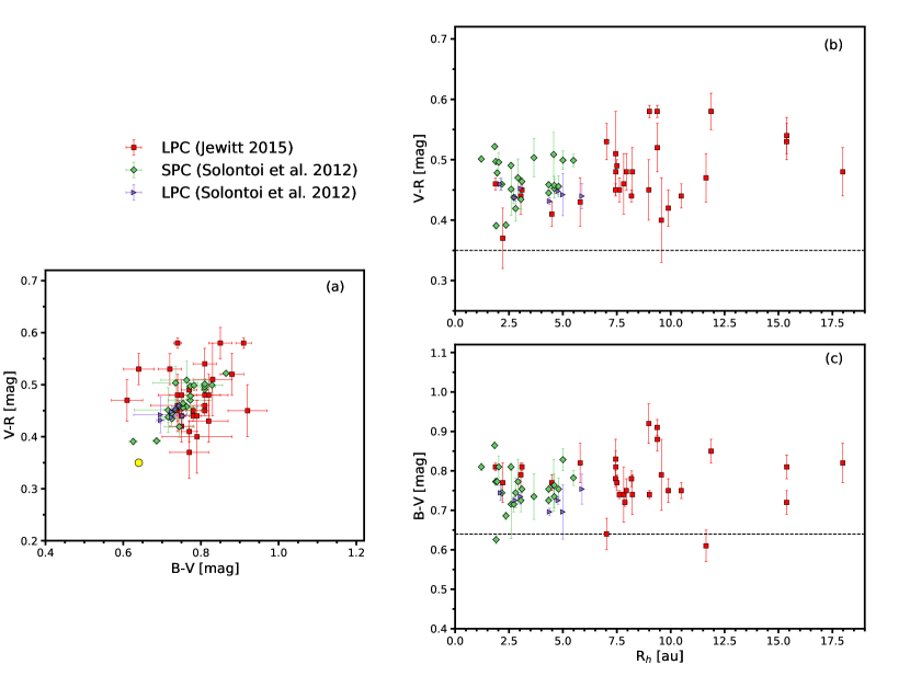
Figure 4: (a) Color–color diagram comparing LPCs from Jewitt (2015) with LPCs and SPCs from the SLOAN survey reported by Solontoi et al. (2012). The color of the Sun is marked by a yellow circle. In (b) and (c) the $V-R$ and $B-V$ colors of the same comets, respectively, is shown as a function of heliocentric distance in au. The dashed horizontal line represents the color of the Sun.

Solontoi et al. (2012) compiled $u$, $g$, $r$, $i$, $z$ band photometry of 26 active comets (6 LPCs and 20 JFCs) observed by the Sloan Digital Sky Survey (SDSS, York et al., 2000) spanning a range of heliocentric distances between $\sim$1 and $\sim$6 au (observations of unresolved comets are not considered). Jewitt (2015) extended the work by Solontoi et al. (2012) by presenting new $B$, $V$, $R$ photometric measurements for 23 active LPCs obtained with the 10 m diameter Keck I telescope at Mauna Kea and the Low Resolution Imaging Spectrometer (LRIS) camera (Oke et al., 1995). This data set not only quadruplicated the number of LPCs for which colors are available, but also broadened the heliocentric distance range with measurements up to 18 au from the Sun. After transforming the measurements by Solontoi et al. (2012) in the Sloan filter system into $BVRI$ photometry (Ivezić et al., 2007), Jewitt (2015) investigated possible correlations between optical colors and orbital parameters for the combined SDSS+Keck data set (see Figure 4). No significant difference was found between the mean colors of active SPCs and LPCs (Figure 4, panel a), suggesting the lack of compositional variation between these two groups. The author pointed out the agreement between this finding and gas-phase studies reported by A’Hearn et al. (2012) and Cochran et al. (2015) and attributed it to the idea, already put forth by A’Hearn et al. (2012), that JFCs and LPCs formed in largely overlapping regions of the protoplanetary disk.

No trend was found between the $B-V$ and $V-R$ colors and heliocentric distance ($R_{h}$, Figure 4, panels b and c). Jewitt (2015) attributed this evidence to 1) ice-to-dust ratio being on the order of only a few percent and 2) small particles not being abundant enough to dominate the scattering cross section. The first conclusion relies on the idea that solid state water has been detected in cometary comae (Davies et al., 1997; Kawakita et al., 2004; Yang et al., 2014; Protopapa et al., 2018), it is stable at large heliocentric distances with sublimation rates varying inversely with heliocentric distance and it is bluer than refractory materials. Therefore, an ice-to-dust ratio larger than few percent would lead to bluer colors with increasing heliocentric distance, contrary to what was observed. The second conclusion leans upon the expectation that, at large heliocentric distances, given the lower gas flow, the mean size of the ejected particles should fall into the Raleigh regime ($X=\pi D/\lambda<<1$, where $D$ is the particle diameter and $\lambda$ is the wavelength of observation), yielding to blue colors (Bohren and Huffman, 1983). However, Gundlach et al. (2015) found, through numerical modeling and laboratory results, that the size range of the dust aggregates able to escape from a comet nucleus into space widens when the comet approaches the Sun and narrows with increasing heliocentric distance. This is because the tensile strength of the dust aggregates decreases with increasing aggregate size. Therefore, at large heliocentric distances, given the lower gas flow, only large aggregates would be lifted off the nucleus. These arguments, which rely on the assumption that comets have formed by gravitational instability (Skorov and Blum, 2012; Blum et al., 2014), weaken the conclusion that small particles are not abundant enough to dominate the scattering cross section.

Not all broad-band comet surveys provide color information, but still measure activity and dust production. Sárneczky et al. (2016) measured A$f\rho$ values and the coma slope parameters for 50 LPCs with known activity beyond 5 au. The $Af\rho$ quantity is the product of albedo ($A$), filling factor of the grains within the field of view ($f$), and the linear radius of the field of view at the comet ($\rho$), while the slope parameter is defined as $d$ log A$f\rho$ / $d$ log $\rho$ (A’Hearn et al., 1984). These parameters are diagnostic of the comet activity and are a proxy for the dust production rate and the morphological appearance of the coma. Sárneczky et al. (2016) divided the LPC sample into dynamically new ($a>10^{4}$ au) and returning comets, and found that on average the A$f\rho$ of dynamically new comets significantly exceed those of the recurrent LPCs, similar to the earlier work of Meech et al. (2009) with a smaller sample. Furthermore they found that new comets usually exhibit negative (shallow) slope ($d$ log A$f\rho$ / $d$ log $\rho$) parameters, and symmetric comae. The comets which were strongly active beyond 10 au, they found, tend to have a smaller increase in A$f\rho$ with decreasing heliocentric distance.

2.2 Thermal dust

Analogously to the $Af\rho$ parameter introduced by A’Hearn et al. (1984, see Section 2.1) as a proxy for the dust production rate measured at visible wavelengths for scattered light observations, Kelley et al. (2013) used the $\epsilon f\rho$ parameter for observations of thermal emission from comet comae introduced by Lisse et al. (2002). The effective emissivity of the grains is parametrized by $\epsilon$, while $f$ is the areal filling factor within an observed aperture of radius $\rho$. Bauer et al. (2015) carried out a comparison between the log $\epsilon f\rho$ as derived from the WISE W3 (12 $\mu$m) and W4 (22 $\mu$m) channel dust emission and the log $Af\rho$ values derived from the W1 (3.4 $\mu$m) channel assuming dust signal was dominated by reflectance. For the comets observed at heliocentric distances exceeding 3 au, the difference between the values ($\sim 0.86\pm 0.1)$ were found to be consistent with dark dust with emissivity near 0.9. Comets observed at heliocentric distances inside 3 au deviated from this trend, possibly owing to the different size range of aggregates lifted by activity at smaller rather than larger heliocentric distances, given the higher gas flow, or to the more pronounced thermal emission component within the 3.4 $\mu$m band signal for the dust at small distances. Outside of 3 au, the sample was dominated by LPCs; only 4 SPCs were measured outside of 3 au.

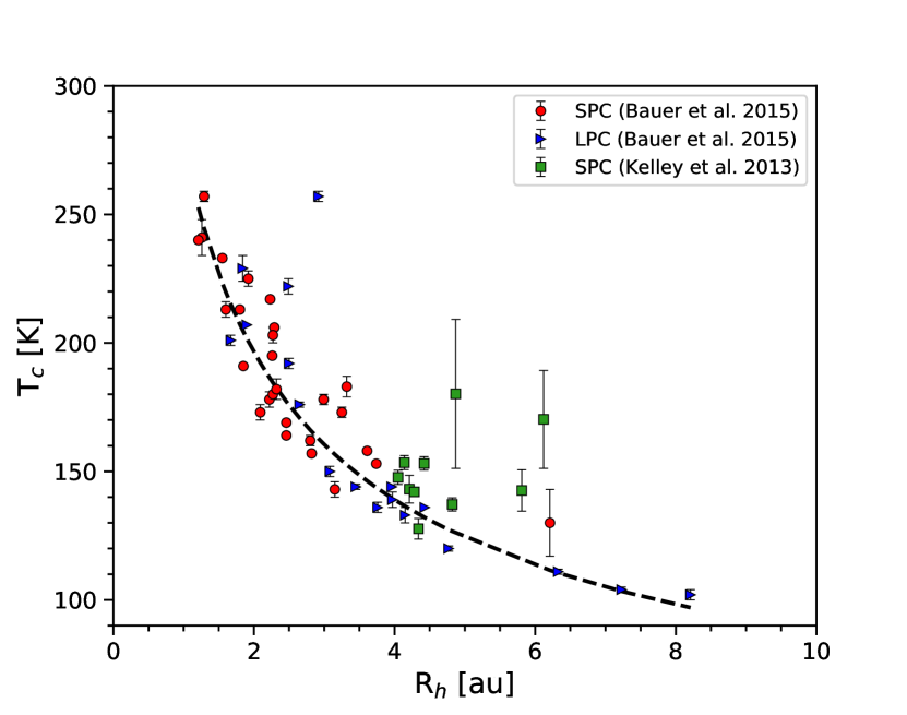
Figure 5: Coma color temperatures as a function of heliocentric distance comparing LPCs from Bauer et al. (2015) with SPCs reported by Bauer et al. (2015) and Kelley et al. (2013, only color temperatures of the dust centered on cometary nuclei are shown). The dashed line represents the temperature of an isothermal blackbody ($278R_{h}^{-1/2}$).

The physical temperature of cometary dust grains is a function of composition, grain size and morphology. An approximation for the true physical temperature of the grains is given by the color temperature $T_{c}$ determined through analysis of the thermal spectral energy distribution over a defined wavelength range (e.g., Wooden, 2002; Kolokolova et al., 2004). The temperature excess of a cometary coma over that of a blackbody is usually parameterized by the superheat parameter $S_{heat}$ introduced by Gehrz and Ney (1992) and defined as the ratio of the color temperature and the temperature of an isothermal blackbody sphere in LTE at the same heliocentric distance ($T_{BB}=278R_{h}^{-1/2}$). Bauer et al. (2015) reported color dust temperatures based on the WISE W3 and W4 band thermal fluxes for 24 SPCs and 14 LPCs while Kelley et al. (2013) reported color temperatures for 15 SPCs through analysis of the 16- and 22-$\mu$m Spitzer Space Telescope MIPS observations (Fig. 5). No differences were found between SPCs and LPCs (Bauer et al., 2015). Overall, cometary comae color temperatures measured with WISE displayed a slight excess of 1.6 $\pm$ 0.1% (the error-weighted mean of all the superheat measurements is $\bigl{\langle}T_{c}/T_{BB}\bigr{\rangle}=1.016\pm 0.001$) and were found to be consistent with isothermal bodies with emissivity $\sim$0.9 and albedo 0.1 at 3.4 $\mu$m (Bauer et al., 2015). A more significant temperature excess was found by Kelley et al. (2013), who reported an error-weighted mean of all their color-temperature measurements of $\bigl{\langle}T_{c}/T_{BB}\bigr{\rangle}=1.074\pm 0.006$. This translates in the color temperature of the dust to be 7.4 $\pm$ 0.6% warmer on average than an isothermal blackbody sphere in LTE. An important caveat to consider when assessing the validity of color temperatures obtained from broad-band infrared photometry is the possible presence of emission features, specifically silicate features, above the continuum which could affect the thermal flux measurements and consequently, the color temperature estimates. Therefore, to properly characterize the thermal properties of cometary grains, spectroscopic data of a large number of comets are required. Sitko et al. (2004) analyzed spectroscopic data over the wavelength range 3-14 $\mu$m of 20 comets belonging to different dynamical classes and found cometary grains radiating at temperatures in excess of that of a blackbody at the equilibrium temperature expected for their heliocentric distances. This effect is expected for a grain population that includes a significant fraction of the grains with sizes smaller than the wavelength of light being radiated, in this case from 3 to 14 $\mu$m. Additionally, Sitko et al. (2004) found a strong correlation between excess temperature and silicate band strength for dynamically new and long-period comets, confirming the results by Gehrz and Ney (1992) and Williams et al. (1997). The majority of Jupiter family objects were found to deviate from this relation. To explain the different trend between JFCs and dynamically new comets, the authors put forth the idea of a radial gradient in the size distribution of silicate grains within the protoplanetary disk. Further observations are required to confirm this finding.

Mid-IR broadband images of comets were found to be well suited not only for characterizing the properties of the dust grains but also to investigate the activity level of comets. Kelley et al. (2013) using Spitzer Space Telescope images acquired as part of the SEPPCoN survey, investigated the activity of 89 JFCs at 3–7 AU from the Sun and found that activity, detected in at least $\approx 24\%$ of the comet sample, is significantly biased to post-perihelion epochs. Additionally, Kelley et al. (2013) suggested a bias in the discovered JFC population given that low-activity comets with large perihelion distances were found missing from the survey sample. The link between activity level and present and historical orbital parameters was also investigated by Mazzotta Epifani et al. (2009) through analysis of a sample of 90 SPCs as seen from the ground and space at heliocentric distances greater than 3 au. This analysis led to several findings including, but not limited to, the higher likelihood of SPCs being active post-perihelion rather than pre-perihelion, similarly to what was found by Kelley et al. (2013), the lack of a sharp cut-off in heliocentric distance marking the activity-fade, and a weak trend of comets with increasing perihelion distance to be more likely active at large heliocentric distance.

Not all analyses of thermal dust is based on flux measures. Reach et al. (2007) conducted a survey of 34 JFCs at 24 $\mu$m using the Spitzer Space Telescope’s Multiband Imaging Photometer for Spitzer (MIPS), and found that the majority (27) of the comets exhibited detectable trails. 2009IshiguroTrails confirmed the prevalence of JFC-associated dust trails, and found that 6 out of 42 Jupiter Family comets exhibited trails detectable at visual-band wavelengths. By over-plotting zero-velocity syndynes (cf. Finson and Probstein 1968), Reach et al. (2007) found that the dust particles were dominated by mm and cm-sized dust, and that the size distribution of the dust particles is not accurately modeled by a single power-law. Kramer et al. (2017) and Kramer (2014) demonstrated a novel technique of fitting the cometary dust in the thermal infrared observations using WISE/NEOWISE data. Subsequent application of the technique (Kramer et al., 2015) to a sample of 89 comets shows that such techniques can elucidate the behavior of dust output of comets when they are most active. Using radiation pressure to sift the different ranges of particle sizes in the tail in combination with the dust thermal signal, they found that much of the dust is emitted preceding perihelion, and that the dust mass is primarily residing in millimeter to centimeter sized grains.

3 SURVEYS OF COMETARY GAS

By nature cometary gas surveys are slow, requiring multi-year commitments to observing the same sorts of objects as they become available one at a time. Whether waiting for a comet bright enough, close enough, or the right phase angle, there may only be one or two comets available per year for which a detailed study of multiple species is feasible. Spacecraft visits may show us a snapshot, but the long term surveys of composition have been critical to telling us what comets have in common, when a snapshot observation is surprising or different, and are beginning to help us understand how comets evolve. Surveys of cometary gas have been critical to the development of our understanding of what comets are, what they are made of and how that composition relates to the origin of our Solar System. The history of how surveys of cometary gas have shaped our understanding of comets is already well summarized by Cochran et al. (2015), Bockelée-Morvan et al. (2015), as well as Biver et al. (this work) so here we shall only note a few key points and recent developments.

3.1 Ground-based Surveys

Early optical spectroscopic surveys are what told us that while all comets contained the same molecular species, that those species came in differing abundances. This led to what has become the grail of modern cometary gas studies: whether there are compositional classes of comets that can be tied to dynamical origin, and thus constrain our knowledge of the composition and temperatures in the protoplanetary disk. The promising early results of A’Hearn et al. (1995) demonstrated that there exits class of comets, dominated by JFCs, that are depleted in carbon-chain molecules. They were followed by multiple groups confirming this result, though finding enough OCCs in the carbon-depleted class that the tie between depletion and dynamical origin is clearly not a simple one (Cochran et al. 2012; Fink 2009; Langland-Shula and Smith 2011; Bair and Schleicher 2021). Infrared and millimiter wave surveys have made the picture more complicated with no consensus on a classification scheme (c.f. the compilations of Mumma and Charnley (2011), Bockelée-Morvan and Biver 2017, and Dello Russo et al. 2016), but new analyses of some of these observations such as that of Lippi et al. (2021) are beginning to find ways to disentangle the numerous abundances and find patterns.

Lippi et al. (2021) also demonstrate the necessity of continued surveys in the IR and sub-millimeter wavelength regimes. The authors admit significant limitations to the 20 comets within their survey (or the 33 in Dello Russo et al. 2016). Harrington Pinto et al. (2021) is working to compile matched observation of comets with CO and CO₂ production rate constraints. Yet, Lippi et al. (2021) affirm that presently, the overlapping samples across optical through the sub-mm are too sparse to deconvolve compositional states from cometary origin and evolutionary effects. In order to successfully make sense of the compositional trends, the species detectable over the full range of wavelengths must be characterized for numbers of comets comparable to those where optical spectroscopic analyses are presently available.

While we generally think of gas surveys as a means to understand relative composition, the physical state of the gas species is a key detail in understanding comet comae as well. Outflow velocity is a critical characteristic in determining gas production rates, dissociation scales, and total mass loss. Line-of-sight velocity of the gas can be measured via spectroscopy done at sufficient resolution to detect doppler line broadening of emission lines. Since coma gas velocity is generally close to $\sim 1$ km/s, sufficient velocity resolution is currently achievable with ground based observing via radio observations at submillimeter and longer wavelengths. Furthermore, when radio spectroscopy includes spatial mapping, and observations are made at a 90 degree phase angle the survey can distinguish potential asymmetries in sunward and anti-sunward outgassing velocities. In their survey mapping the OH coma at 18 cm in 28 comets Lovell and Howell (2015) found the gas outflow velocity beyond 1 au was 0.8 km/s regardless of size, production rate or direction. While at this time the Atacama Large Millimeter/submillimeter Array (ALMA) is still too new for there to be enough observations of comets to qualify as a survey: it’s potential to spatially map both coma compositions and velocities will produce a unique survey to look forward to.

3.2 Spacecraft Surveys

The advantages of spacecraft are clear, and partially addressed in section1, but for the purposes of studying gas production have additional advantages. The often higher resolution provided by space platforms can facilitate the measurement of product decay scales and associations with nucleus orientations and features (c.f. Fougere et al. 2016), However, space-based telescopes and instruments are often designed with both solar system and non solar system targets in mind. Hence, band-passes, resolution, and spatial scales may be only moderately suited to the measurements used to place constraints on the given species.

The Solar Wind ANisotropies (SWAN) instrument on the SOHO spacecraft, for example, was designed to measure H-alpha line emission associated with large scale structures in the solar wind (Bertaux et al., 1995). However, comets manifest h-alpha emission, $90\%$ of which is produced by water dissociation mechanisms. Hence, SOHO’s SWAN instrument has been effectively used to measure pre- and post-perihelion production of water in 61 comets (Combi et al., 2019). These have provided power-law relationships for water production ($Q_{H2O}$) vs. heliocentric distance ($R_{h}$) in 44 LP and 17 SP comets. Combi et al. (2011) demonstrated the methodology employed in the analysis. Power law fits were provided for the pre and post perihelion approaches of the comets using the relation:

$$Q_{H2O}=Q_{{}_{1AU}}{R_{h}}^{p}$$ (1)

where Q_1AU is the water production rate extrapolated to when the comet is at $R_{h}=1AU$, and p is the ”slope” parameter (manifested as a slope in log units). Comparisons were made of the water production slopes according to dynamical sub-classes of LPCs, dynamically new OCCs (with semi-major axis values greater than 20000AU), and SPCs, and compositional sub-classes of ”carbon-depleted” and ”typical” LPCs and SPCs (A’Hearn et al., 1995). The dynamically new OCCs or younger comets tended to have less variation in slope values, clustering around values of $\sim-2\pm 1$, and exhibited a possible steepening in slope as LPCs dynamically aged. For short-period comets with measured nucleus effective radius values, larger fractional active area correlated with comets with larger perihelion distances, consistent with less processing. The correlations with compositional classifications, and LP pre- and post-perihelion observations, were inconclusive.

Spacecraft observations can provide unique opportunities to assess gas species such as CO₂ which are not available to ground-based observations. CO₂ and CO are two drivers of cometary activity, outpacing water production in a limited range of circumstances, and their out-gassing in these cases provides the dominant means of ejecting dust from the nucleus into the coma. CO can be detected from the ground at sub-millimeter and infrared wavelengths, but this is not the case for CO₂ emission, which is blocked by the absorption of CO₂ present in earth’s own atmosphere. Alternative means of detecting CO₂ are under investigation (e.g. Decock et al. 2013, McKay et al. 2016 and McKay et al. 2019) but direct detection, usually from the 4.26 $\mu$m infrared emission line, is the current means of assessing production rates. Both Spitzer Space Telescope’s Infrared Camera’s (IRAC’s) 4.5 $\mu$m imaging band and the WISE/NEOWISE $4.6\mu$m band contain both the infrared CO₂ and CO ($4.67\mu$m) emission feature. The CO band relative to the CO₂ band is on the order of 11 times weaker. However, without an accompanying CO observation from ground-based assets or spectroscopic data, there is no definitive way to determine which species causes excess in the $\sim 4.5$ micron channels of these two spacecraft. Furthermore, dust thermal emission signal dominates over CO+CO₂ excess at heliocentric distances within $\sim 2$ au. For comets at smaller heliocentric distances, the dust thermal signal must be well-characterized or the emission excess extremely pronounced (or both) for successful detections. That being said, Reach et al. (2013) produced measurements of 23 comets with CO or CO₂ emission using SST, and Bauer et al. (2015) measured 39 comets with CO or CO₂ excess using the WISE/NEOWISE (hereafter NEOWISE) survey data. Reach et al. (2013) attributed the majority of the excess to CO₂ production. Additionally, by comparing with literature measurements of $Q_{H_{2}O}$ the SST survey concluded that water sublimation remained dominant out to $\sim 2.8$ au for most comets, and the highest resolution IRAC images suggested more localized active regions for CO₂ production. The NEOWISE results suggested that approximately a quarter of comets observed had significant CO or CO₂ excess, and a Q${}_{CO_{2}}$ proportionality $\sim{R{{}_{h}}}^{-2}$ within 4 au. Outside 4 au LPCs tended to be the producers of CO or CO₂, and Bauer et al. (2021) attributed that to LPCs possibly being more CO-rich. Recent work by Gicquel et al. (2021) extends these analyses with an additional 52 comets observed by NEOWISE in 2014. It is also important to note that both the SST and NEOWISE surveys referenced the Ootsubo et al. (2012) Akari spacecraft results. Though, with a sample of 18 comets, smaller than the survey number threshold considered here, the attribution of CO₂ as the main species with the SST and NEOWISE surveys was at least in part based on these measurements. Furthermore, the Akari spacecraft spectra provided simultaneous water production comparisons and demonstrated that LPCs were generally producing CO₂ at greater distances and in some instances outpacing water production. About a fifth of the CO₂ producers had CO production that outpaced CO₂ production rates for the Akari-observed sample.

4 SURVEYS OF COMETARY NUCLEI

The basic parameters of nucleus observations have been described by (e.g.) Jewitt (1991), but surveys of nuclei have historically been difficult to perform due to the problem of coma confusion. While we as a field have continued to make good progress on observing nuclei since the time of the predecessor volume, we discuss here some of the effects that can fool us into misinterpreting nucleus photometry and thereby lead to systematic inaccuracies.

For a thorough review of the current understanding of nucleus ensemble properties, we refer the reader to Knight et al. (this volume), who discuss what we currently know about the sizes, shapes, spin states, scattering properties, and thermal properties of nuclei. One overarching result that is clear from such a compilation is that a survey that samples the full diversity of variation, and that samples enough nuclei to drive down the Poisson noise in each sampling bin, is crucial for being able to take the next step in interpreting the distribution in the context of origins and evolutionary processes.

The most fundamental (and ongoing) problem is perhaps that of separating the coma’s flux from the nucleus’s flux. In many cases the comet has an extended coma within which a point-source is embedded, so it is obvious that the comet is showing us not just light from the nucleus. A significant step forward in handling these cases came with the development of empirical coma-fitting routines that could photometrically separate the contributions from nucleus and coma (Lamy et al., 1996, 2004), and such techniques have been used in several nucleus surveys (e.g. Fernández et al., 2013; Bauer et al., 2017). The technique has proven to be successful as evinced by its success at finding the size of nuclei that were then observed directly with resolved imaging by visiting spacecraft (Lamy et al., 1998; Lisse et al., 2009, e.g.). The limitation of this technique arises when the contrast between the nucleus and coma is too low, i.e. if a large fraction of the light in the central pixels is from the coma (Hui and Li, 2018). This can happen if the coma is particularly strong or if the comet is distant. While comets are still most often imaged at visible wavelengths, imaging in the infrared, if the coma is still sufficiently well-detected, is generally more likely to result in a robust extraction (Bauer et al., 2020). For one thing, the most optically-active grains at some infrared wavelengths usually provide less total surface area (for a typical size distribution) than those in the visible. Also, at thermal wavelengths, the nucleus will generally be hotter than the surrounding dust grains (since an area on the nucleus only emits into $2\pi$ sr vs. the $4\pi$ sr dust grains emit into). Both of these effects would tend to increase the nucleus-coma contrast. The other scenario that can be problematic depends on grain outflow dynamics; if the coma’s surface brightness profile at a given azimuth deviates significantly in the inner coma from what is measured in the outer coma, the extrapolation can yield incorrect results. An additional, but related, aspect to this is that the method assumes that the light from the extracted point-source is all from the nucleus, which may not be true. One example of a difficult case is that of C/1995 O1 (Hale-Bopp), where the extreme dust production complicated the extraction of the nucleus’s signal (Fernández, 2002).

There is also the case of a comet that appears as a point-source – and hence one might assume that the comet is inactive – but yet the photometry indicates that there is excess light. The prototypical comet for this situation is comet 2P/Encke (Meech et al., 2001; Fernández et al., 2005). Generally the more distant the comet, where the linear width at the comet of the (angular) point-spread function is larger, the easier it is to hide a dust coma within the seeing disk. However it seems that this phenomenon alone cannot explain the specific situation with 2P/Encke; Presler-Marshall (2021) showed that for a particular dataset (and the observing conditions that went with it) where the comet looked entirely point-source like, only about $\sim$20% of the flux could be from a steady-state $1/\rho$ dust coma. Any more than that would be revealed as wings in the comet’s profile. The analysis did not assess other coma shapes, so it is possible that a large-grain coma, with particles moving below escape velocity around 2P/Encke’s nucleus, could play a role.

Even when one is sure that the light from a comet is all or nearly all from the nucleus, the interpretation can still be muddled if the observation is just a snapshot. The rotational context is often necessary to be sure of what one is actually measuring. Fortunately, this problem is not as terrible as it may seem as first. E.g., Lamy et al. (2004) show that most measurements even without rotational context will still often be within $\sim$90% of the correct answer anyway. Furthermore, for survey data such rotational variations in profile often may be averaged over, as data may span days.

Ideally temporal coverage will extend all around the orbit so as to understand not only the spin period but also the spin axis direction and some shape information. That often presents a problem, since one may only be able to see one region of a nucleus from Earth when the comet is highly active. Of course we now also have much observational evidence that comets change their spin states on orbital (and shorter!) timescales as well , so measurements obtained at multiple epochs may be challenging to fold into each other in the classical ways (e.g. Stellingwerf, 1978).

4.1 Sizes

Assessing the size distribution of cometary nuclei by definition requires an extensive survey, since it can only be measured by having a sufficient number of targets. One significant problem is that there is always a diameter above which the sample is sufficiently representative for a robust analysis. Though that size lower-limit is dependent on the survey’s sensitivity, it is not often clear where that critical diameter is (see also 1.3). A plot of the cumulative size distribution (CSD) of nuclei $N(>D)$ (where $N$ is the number of nuclei with diameter larger than $D$) always shows a flattening at small ($\sim$1-2 km) diameters; equivalently, a plot of the size-frequency distribution (SFD) $n(D)\ dD$ (where $n$ is the number of nuclei with diameter between $D$ and $D+dD$) shows a dropoff toward zero at small diameters. This is at least partially due to the fact that (a) our discovery of such comets is less efficient to begin with, and (b) those are often the very comets for which it is hardest to determine accurate nucleus information because the coma obscures the nucleus signal and/or the nucleus is just too faint. In any case, clearly such a feature of the CSD or SFD adds difficulty when trying to fit, say, a power law.

A more robust solution is to assess what the observational biases are in the discovery of the comets. These observational biases will often lead to one or two effects that can accounted for in the CSD or SFD itself and so will yield a more realistic distribution. This is a challenging task however when comet discoveries are made by a wide range of facilities. For the smallest comets ($\sim$1 km diameter and below) it is especially difficult.

For the JFCs, ideally a survey would either sample a significant fraction of the known comets or make a thorough sweep of the sky to discover the population, including observing the known comets. There must be sufficiently robust software to identify an object as being active. At time of writing there are over 600 JFCs known.

For the LPCs, the additional problem, in contrast to the JFCs, is that the comets are simply not visible for as long a period of time. A JFC will return again and again to provide (at least theoretically) multiple observing chances over several decades. An LPC is viewable throughout its perihelion only once over the lifetime of the survey. The LPCs are often more active than the JFCs as well, making it harder to extract nucleus properties.

Given the number of complications that come with studying nuclei, it may not be surprising that there is some divergence in results regarding the size distribution, and different methodologies complicate the picture. For example, the LPC nucleus distribution reported by Bauer et al. (2017) comes from NEOWISE observations in the infrared and makes use of the coma-extraction technique. Additionally, there is the LPC distribution reported by Boe et al. (2019), which instead comes from visible-wavelength imaging via the ‘nuclear’ absolute magnitudes in JPL’s database, and a model of activity to correct those absolute magnitudes – which generally are not representative of the nucleus alone – for coma contribution. Thus direct comparisons between the two studies could be difficult. Independent estimates of the particular LPCs in the two studies would be a useful check, but such estimates are sparse. It can be noted that a comparison of JFC (not LPC) nucleus diameters in the Bauer et al. (2017) work with those in the SEPPCoN survey (Fernández et al., 2013) and with those from spacecraft encounters show a reasonable match to within 25 percent.

Another potentially useful approach to get around the problem of contaminating coma is to restrict a survey to objects that are known to be inactive or only very weakly active. For example, as part of the overall ExploreNEO survey, Mommert et al. (2015) report observations of several dormant or extinct comets. However the connection between the size distribution of such highly-evolved comets and of the active JFCs is still to be determined. Extinct comets are, by definition, after all the survivors of an active lifetime that for many comets includes significant fragmentation (and thus potentially a large change in size) if not total disintegration.

5 FUTURE SURVEYS OF COMETS

Surveys will continue to be vital for us to probe the ensemble properties of comets and specifically to understand the full diversity of the population. While flybys and rendezvous of specific comets will of course provide detailed studies of such objects and phenomenological first-hand accounts, it is important that the comet community continue to take advantage of ground-based and space-based telescopic assets that can shed light on a representative cometary sample. This includes making use of facilities whose original science drivers lie in the astrophysical or heliophysical realms.

Some facilities that we hope will become active in the 2020s have the potential to bring us a significant jump in the number of known, characterized comets. The Rubin Observatory (c.f. Jones et al. 2009) and NEO Surveyor (Mainzer et al., 2021), which will both be scanning the skies for Solar System objects in the near future, will provide us with the number statistics that would be incredibly helpful. Estimates of the surveys’ efficiencies suggest that we could be finding thousands of new comets (Solontoi et al., 2010; Vera C. Rubin Observatory LSST Solar System Science Collaboration et al., 2020; Sonnett et al., 2021). In particular, we can increase the number of LPCs that are discovered per year, and the number of such comets that are discovered beyond 5 and 10 au, expanding baselines of behavior before activity has ramped up. This will also make it easier for follow-up observations to assess the properties of their nuclei. Another important consideration that number statistics will help with is our understanding of the evolutionary paths of the JFCs. For example, both surveys are supposed to be sensitive enough to sample the sub-kilometer JFC population and we might expect such a population to exist as a result of mass loss and fragmentation over the comets’ lifetimes. However it is also possible such small comets quickly disintegrate all the way to dust. Rubin and NEO Surveyor will extend the number statistics into this size regime. Hence the surveys will be better able to determine how well small comets survive their active lifetimes.

Finally, the two surveys will be very complementary to each other since the combination of visible (reflected) and IR (thermal) wavelength observations, and observations spanning several years at multiple epochs, will be tremendously helpful for gauging gas, dust, and nucleus properties. In a similar vein as WISE/NEOWISE, NEO Surveyor will provide measurements of nucleus sizes, dust characteristics, and CO and CO₂ production of manifold larger statistical samples.

The SPHEREx mission will provide us with near-IR spectroscopic investigations of dozens of comets. Importantly, such data will extend to wavelengths where CO and CO₂ rovibrational bands emit, which means SPHEREx may build upon results of Akari with additional insight into these important species (Doré et al., 2016).

Furthermore low-cost mission concepts could, if brought to fruition, also address highly specific comet-related questions through a survey. In particular cubesats can provide such survey work for relatively low cost. For example a small but fast, wide-field UV telescope in Earth-orbit could let us make measurements of the OH electronic band near 309 nm in hundreds of cometary comae. Such a database, with observations covering all dynamical types, and covering a range of heliocentric distances, and used in concert with dust production measurements, could give a simple test of just how and when the water production is tied to dust. Cubesats could also be employed for an in situ survey of multiple comets. For example, equipping a fleet of cubesats with replicas of the MIRO instrument on Rosetta, and sending them out to a few dozen comets in the inner Solar System, would give us unprecedented views of cometary near-surface interiors and let us assess how void space and consolidation evolve as a comet ages through its active lifetime.

A survey with the James Webb Space Telescope (JWST) has the potential to let us take the next step in our understanding of the comet population’s nuclei, gas production, and dust production. It will provide more detailed gas production measurements, at a larger range of heliocentric distances, and for a broader range of species (especially parent species), than ever before. We will be able to watch the changing release of various volatiles over time as a comet approaches and recedes from the Sun, and do it not just for exceptional comets such as Hale-Bopp, but for more typical comets and comets from all dynamical classes and ages. Similar synoptic coverage of the thermal and scattering properties of the dust as the comet moves in its orbit will likewise let us investigate how the grain properties change in response to the activity driver, giving clues about the nature of the ice-rock mixture in cometary subsurface layers. This will come from not only spectroscopic assessment of the dust spectral energy distribution (and its resulting decomposition into mineralogy) but also from resolved imaging of the dust coma. JWST’s stable point-spread-function and high spatial resolution will give us the best chance of overcoming the coma confusion problem, and let us do so at a range of wavelengths, thereby letting us have a better handle on overall thermal emission from the nucleus. Being able to do all this for 20 to 30 comets would be spectacular.

There are of course many additional, large-scale space telescopes in various levels of planning/concreteness that would theoretically arrive in the decades of the 2030s and 2040s. The Roman Space Telescope, for example, will provide multiband red and near-IR imaging of cometary dust, as well as grism spectroscopy that covers the 1.5 micron water ice absorption band, thus potentially providing a survey of icy grains (Holler et al., 2018). In the more distant future, observatories like the Large Ultraviolet Optical Infrared Surveyor (LUVOIR) or the Origins Space Telescope (c.f. National Academies of Sciences, Engineering, and Medicine 2021) would further expand the samples. These observatories, combining significant improvements in sensitivity with high-resolution imaging and spectroscopy, may be used to get a statistical sense of the nature of low-level activity in comets at large heliocentric distances, as well as obtain large samples of surface constituents via spectroscopic studies, and explore the presence of other possible drivers of activity, like methane, at larger distances (cf. Meech and Svoren 2004 and Brown 2000). Such facilities, if capable of non-sidereal tracking, would certainly provide a new jump in our understanding of comets by taking us to the next level of detail on dozens to hundreds of these bodies.

Radio-wavelength surveys with existing high-spatial resolution facilities like ALMA and with future facilities like the next generation Vary Large Array, ngVLA, and the Next Generation Arecibo Telescope (NGAT) (Roshi et al., 2019) will provide great insight into energetics of the gas coma. The NGAT would also have a phased radar capability and thus provide a significantly higher power output that has been previously possible. This would allow us to obtain more detailed pictures of the large-grain (cm-scale) dust coma as well as the nucleus structure on cm-scales. The number of radar-detected comets has slowly increased since the predecessor volume, and is still fairly small, so a boost to the emitted power could drastically increase the number of available comets that could be sampled in this way. Radio continuum measurements (in passive mode) at a variety of sub-mm, mm, and cm wavelengths would let us sample different depths in a nucleus, down to approximately a meter. This has already been demonstrated with ALMA with observations of Ganymede (de Kleer et al., 2021). Again, an assessment of the surface and sub-surface properties of a range of nuclei of varying ages and activity levels could be insightful.

There are many excellent surveys of cometary properties that are discussed throughout the current volume and the predecessor volume. But often the statistics could be improved to sharpen the conclusions by observing more comets or by observing the same comets in more detail (e.g. better temporal coverage, wavelength coverage, spatial resolution, or spectral resolution). With growing data sets, selecting the necessary qualities of the data to undertake analyses of physical properties, and tailor selections to particular sub-populations, will require improved meta-data. Complex information models as the basis of meta-data, like PDS4 (Raugh and Hughes, 2021) and the Minor Planet Center’s new Astrometry Data Exchange Standard (ADES; Chesley et al. 2017), which are associated with archived data, will facilitate these applications and analyses. The meta-data labels and automated tools will allow users to identify and extract the desired data for analysis. The question of when one has ‘enough’ samples to draw a conclusion at a sufficient confidence level is not easy to answer ahead of time unless one has a good sense of the inherent diversity in the population.

6 SUMMARY

Surveys have had a large impact on our knowledge base of comets. They provide a systematical approach towards collecting large samples of data reflective of cometary physical characteristics and behavior and more revealing of the comprehensive cometary object populations. It is important to also acknowledge that comet science can advance as well with surveys done by telescopic assets that may have primarily astrophysical or heliophysical science drivers, and we advocate for the continued use of such facilities. We also would like to see that those facilities that are open to general observers for targeted observations accommodate at least some of the non-sidereal tracking capability that is so important for Solar System science.

Some key features in the sky survey analysis approaches include:

1. most comets are now discovered by all-sky surveys, SLSs and TPSs.

2. the majority of yearly detections are also made by such surveys.

3. critical margins remain outside survey coverage which create opportunities for targeted single-object observations and non-survey discovery of unique cometary objects.

4. the data from sky surveys are well-explored for discovery and astrometric measurements, while only cursorily exploited as a resource for physical and behavior characterization.

For targeted larger-sample surveys:

1. larger-sample sizes, the expanse of sample, and broadening of wavelength regimes will lead to more comprehensive understanding of compositional variations across orbit classes and sub-classes, and separate original composition from evolutionary effects.

2. characterizing the physical states of comet components (e.g. gas phase, tail dust, nucleus spin, etc.) remains in the early stages of large-sample collection.

Larger-scale surveys in general will lead to improved earth-space situational awareness, understanding of the evolutionary processing of comets and solar system volatile transport, as well as solar system formation. Finally, future larger-scale surveys will require the use of advanced astro-informatic techniques and incorporation of AI routines to realistically process the increased data volume.

Acknowledgments.

JMB and YRF acknowledge support from the NEO Surveyor mission, funded by NASA Contract 80MSFC20C0045. YRF also acknowledges support from the Center for Lunar and Asteroid Surface Science, funded by NASA Contract 80NSSC19M0214. We acknowledge helpful discussions with A. Lovell that improved this chapter.

References

- A’Hearn et al. (2012) A’Hearn M. F., Feaga L. M., Keller H. U., Kawakita H., Hampton D. L., Kissel J., Klaasen K. P., McFadden L. A., Meech K. J., Schultz P. H., Sunshine J. M., Thomas P. C., Veverka J., Yeomans D. K., Besse S., Bodewits D., Farnham T. L., Groussin O., Kelley M. S., Lisse C. M., Merlin F., Protopapa S., and Wellnitz D. D. (2012) Cometary Volatiles and the Origin of Comets, ApJ, 758, 29.
- A’Hearn et al. (1995) A’Hearn M. F., Millis R. C., Schleicher D. O., Osip D. J., and Birch P. V. (1995) The ensemble properties of comets: Results from narrowband photometry of 85 comets, 1976-1992., Icarus, 118, 223–270.
- A’Hearn et al. (1984) A’Hearn M. F., Schleicher D. G., Millis R. L., Feldman P. D., and Thompson D. T. (1984) Comet Bowell 1980b, AJ, 89, 579–591.
- Bair and Schleicher (2021) Bair A. N. and Schleicher D. G. (2021) in AAS/Division for Planetary Sciences Meeting Abstracts, vol. 53 of AAS/Division for Planetary Sciences Meeting Abstracts, p. 210.03.
- Battams and Boonplod (2020) Battams K. and Boonplod W. (2020) C/2020 X3 (SOHO), Minor Planet Electronic Circulars, 2020Y19.
- Battams and Knight (2017) Battams K. and Knight M. M. (2017) SOHO comets: 20 years and 3000 objects later, Philosophical Transactions of the Royal Society of London Series A, 375, 20160257.
- Bauer et al. (2020) Bauer J., Gicquel A., Kramer E., Mainzer A., Masiero J., Fernandez Y., Schambeau C., Stevenson R., Lisse C., Meech K., and NEOWISE Team (2020) in AAS/Division for Planetary Sciences Meeting Abstracts, vol. 52 of AAS/Division for Planetary Sciences Meeting Abstracts, p. 316.04.
- Bauer et al. (2021) Bauer J. M., Gicquel A., Kramer E., and Meech K. J. (2021) NEOWISE Observed CO and CO2 Production Rates of 46P/Wirtanen During the 2018-2019 Apparition, \psj, 2, 34.
- Bauer et al. (2017) Bauer J. M., Grav T., Fernández Y. R., Mainzer A. K., Kramer E. A., Masiero J. R., Spahr T., Nugent C. R., Stevenson R. A., Meech K. J., Cutri R. M., Lisse C. M., Walker R., Dailey J. W., Rosser J., Krings P., Ruecker K., Wright E. L., and NEOWISE Team (2017) Debiasing the NEOWISE Cryogenic Mission Comet Populations, AJ, 154, 53.
- Bauer et al. (2015) Bauer J. M., Stevenson R., Kramer E., Mainzer A. K., Grav T., Masiero J. R., Fernández Y. R., Cutri R. M., Dailey J. W., Masci F. J., Meech K. J., Walker R., Lisse C. M., Weissman P. R., Nugent C. R., Sonnett S., Blair N., Lucas A., McMillan R. S., Wright E. L., WISE t., and NEOWISE Teams (2015) The NEOWISE-Discovered Comet Population and the CO + CO2 Production Rates, ApJ, 814, 85.
- Bertaux et al. (1995) Bertaux J. L., Kyrölä E., Quémerais E., Pellinen R., Lallement R., Schmidt W., Berthé M., Dimarellis E., Goutail J. P., Taulemesse C., Bernard C., Leppelmeier G., Summanen T., Hannula H., Huomo H., Kehlä V., Korpela S., Leppälä K., Strömmer E., Torsti J., Viherkanto K., Hochedez J. F., Chretiennot G., Peyroux R., and Holzer T. (1995) SWAN: A Study of Solar Wind Anisotropies on SOHO with Lyman Alpha Sky Mapping, Sol. Phys., 162, 403–439.
- Blum et al. (2014) Blum J., Gundlach B., Mühle S., and Trigo-Rodriguez J. M. (2014) Comets formed in solar-nebula instabilities! - An experimental and modeling attempt to relate the activity of comets to their formation process, Icarus, 235, 156–169.
- Bockelée-Morvan and Biver (2017) Bockelée-Morvan D. and Biver N. (2017) The composition of cometary ices, Philosophical Transactions of the Royal Society of London Series A, 375, 20160252.
- Bockelée-Morvan et al. (2015) Bockelée-Morvan D., Calmonte U., Charnley S., Duprat J., Engrand C., Gicquel A., Hässig M., Jehin E., Kawakita H., Marty B., Milam S., Morse A., Rousselot P., Sheridan S., and Wirström E. (2015) Cometary Isotopic Measurements, Space Sci. Rev., 197, 47–83.
- Bodewits et al. (2007) Bodewits D., Christian D. J., Torney M., Dryer M., Lisse C. M., Dennerl K., Zurbuchen T. H., Wolk S. J., Tielens A. G. G. M., and Hoekstra R. (2007) Spectral analysis of the Chandra comet survey, A&A, 469, 1183–1195.
- Boe et al. (2019) Boe B., Jedicke R., Meech K. J., Wiegert P., Weryk R. J., Chambers K. C., Denneau L., Kaiser N., Kudritzki R. P., Magnier E. A., Wainscoat R. J., and Waters C. (2019) The orbit and size-frequency distribution of long period comets observed by Pan-STARRS1, Icarus, 333, 252–272.
- Bohren and Huffman (1983) Bohren C. F. and Huffman D. R. (1983) Absorption and scattering of light by small particles.
- Bonnet and Wright (2000) Bonnet D. G. and Wright T. A. (2000) Sample size requirements for estimating pearson, kendall and spearman correlations., Psychometrika, 65, 23–28.
- Borisov and Shustov (2021) Borisov G. V. and Shustov B. M. (2021) Discovery of the First Interstellar Comet and the Spatial Density of Interstellar Objects in the Solar Neighborhood, Solar System Research, 55, 124–131.
- Borne et al. (2009) Borne K., Accomazzi A., Bloom J., Brunner R., Burke D., Butler N., Chernoff D. F., Connolly B., Connolly A., Connors A., Cutler C., Desai S., Djorgovski G., Feigelson E., Finn L. S., Freeman P., Graham M., Gray N., Graziani C., Guinan E. F., Hakkila J., Jacoby S., Jefferys W., Kashyap, Kelly B., Knuth K., Lamb D. Q., Lee H., Loredo T., Mahabal A., Mateo M., McCollum B., Muench A., Pesenson M., Petrosian V., Primini F., Protopapas P., Ptak A., Quashnock J., Raddick M. J., Rocha G., Ross N., Rottler L., Scargle J., Siemiginowska A., Song I., Szalay A., Tyson J. A., Vestrand T., Wallin J., Wandelt B., Wasserman I. M., Way M., Weinberg M., Zezas A., Anderes E., Babu J., Becla J., Berger J., Bickel P. J., Clyde M., Davidson I., van Dyk D., Eastman T., Efron B., Genovese C., Gray A., Jang W., Kolaczyk E. D., Kubica J., Loh J. M., Meng X.-L., Moore A., Morris R., Park T., Pike R., Rice J., Richards J., Ruppert D., Saito N., Schafer C., Stark P. B., Stein M., Sun J., Wang D., Wang Z., Wasserman L., Wegman E. J., Willett R., Wolpert R., and Woodroofe M. (2009) in astro2010: The Astronomy and Astrophysics Decadal Survey, vol. 2010, p. P6.
- Brown (2000) Brown M. E. (2000) Near-Infrared Spectroscopy of Centaurs and Irregular Satellites, AJ, 119, 977–983.
- Chesley et al. (2017) Chesley S. R., Hockney G. M., and Holman M. J. (2017) in AAS/Division for Planetary Sciences Meeting Abstracts #49, vol. 49 of AAS/Division for Planetary Sciences Meeting Abstracts, p. 112.14.
- Cochran et al. (2012) Cochran A. L., Barker E. S., and Gray C. L. (2012) Thirty years of cometary spectroscopy from McDonald Observatory, Icarus, 218, 144–168.
- Cochran et al. (2015) Cochran A. L., Levasseur-Regourd A.-C., Cordiner M., Hadamcik E., Lasue J., Gicquel A., Schleicher D. G., Charnley S. B., Mumma M. J., Paganini L., Bockelée-Morvan D., Biver N., and Kuan Y.-J. (2015) The Composition of Comets, Space Sci. Rev., 197, 9–46.
- Combi et al. (2011) Combi M. R., Lee Y., Patel T. S., Mäkinen J. T. T., Bertaux J. L., and Quémerais E. (2011) SOHO/SWAN Observations of Short-period Spacecraft Target Comets, AJ, 141, 128.
- Combi et al. (2019) Combi M. R., Mäkinen T. T., Bertaux J. L., Quémerais E., and Ferron S. (2019) A survey of water production in 61 comets from SOHO/SWAN observations of hydrogen Lyman-alpha: Twenty-one years 1996-2016, Icarus, 317, 610–620.
- Davies et al. (1997) Davies J. K., Roush T. L., Cruikshank D. P., Bartholomew M. J., Geballe T. R., Owen T., and de Bergh C. (1997) The Detection of Water Ice in Comet Hale-Bopp, Icarus, 127, 238–245.
- de Kleer et al. (2021) de Kleer K., Butler B., de Pater I., Gurwell M. A., Moullet A., Trumbo S., and Spencer J. (2021) Ganymede’s Surface Properties from Millimeter and Infrared Thermal Emission, \psj, 2, 5.
- Decock et al. (2013) Decock A., Jehin E., Hutsemékers D., and Manfroid J. (2013) Forbidden oxygen lines in comets at various heliocentric distances, A&A, 555, A34.
- Dello Russo et al. (2016) Dello Russo N., Kawakita H., Vervack R. J., and Weaver H. A. (2016) Emerging trends and a comet taxonomy based on the volatile chemistry measured in thirty comets with high-resolution infrared spectroscopy between 1997 and 2013, Icarus, 278, 301–332.
- Dennerl et al. (1997) Dennerl K., Englhauser J., and Trümper J. (1997) X-ray emissions from comets detected in the Röntgen X-ray satellite all-sky survey., Science, 277, 1625–1630.
- Dobson et al. (2021) Dobson M. M., Schwamb M. E., Fitzsimmons A., Kelley M. S. P., Lister T., Shingles L. J., Denneau L., Heinze A. N., Smith K. W., Tonry J. L., Weiland H., Young D. R., Benecchi S. D., and Verbiscer A. J. (2021) New or Increased Cometary Activity in (2060) 95P/Chiron, Research Notes of the American Astronomical Society, 5, 211.
- Doré et al. (2016) Doré O., Werner M. W., Ashby M., Banerjee P., Battaglia N., Bauer J., Benjamin R. A., Bleem L. E., Bock J., Boogert A., Bull P., Capak P., Chang T.-C., Chiar J., Cohen S. H., Cooray A., Crill B., Cushing M., de Putter R., Driver S. P., Eifler T., Feng C., Ferraro S., Finkbeiner D., Gaudi B. S., Greene T., Hillenbrand L., Höflich P. A., Hsiao E., Huffenberger K., Jansen R. A., Jeong W.-S., Joshi B., Kim D., Kim M., Kirkpatrick J. D., Korngut P., Krause E., Kriek M., Leistedt B., Li A., Lisse C. M., Mauskopf P., Mechtley M., Melnick G., Mohr J., Murphy J., Neben A., Neufeld D., Nguyen H., Pierpaoli E., Pyo J., Rhodes J., Sandstrom K., Schaan E., Schlaufman K. C., Silverman J., Su K., Stassun K., Stevens D., Strauss M. A., Tielens X., Tsai C.-W., Tolls V., Unwin S., Viero M., Windhorst R. A., and Zemcov M. (2016) Science Impacts of the SPHEREx All-Sky Optical to Near-Infrared Spectral Survey: Report of a Community Workshop Examining Extragalactic, Galactic, Stellar and Planetary Science, arXiv e-prints, arXiv:1606.07039.
- Farnham et al. (2021) Farnham T., Kelley M., and Bauer J. (2021) in AAS/Division for Planetary Sciences Meeting Abstracts, vol. 53 of AAS/Division for Planetary Sciences Meeting Abstracts, p. 301.06.
- Farnham et al. (2019) Farnham T. L., Kelley M. S. P., Knight M. M., and Feaga L. M. (2019) First Results from TESS Observations of Comet 46P/Wirtanen, ApJ, 886, L24.
- Fernández (2002) Fernández Y. R. (2002) The Nucleus of Comet Hale-Bopp (C/1995 O1): Size and Activity, Earth Moon and Planets, 89, 3–25.
- Fernández et al. (2013) Fernández Y. R., Kelley M. S., Lamy P. L., Toth I., Groussin O., Lisse C. M., A’Hearn M. F., Bauer J. M., Campins H., Fitzsimmons A., Licandro J., Lowry S. C., Meech K. J., Pittichová J., Reach W. T., Snodgrass C., and Weaver H. A. (2013) Thermal properties, sizes, and size distribution of Jupiter-family cometary nuclei, Icarus, 226, 1138–1170.
- Fernández et al. (2005) Fernández Y. R., Lowry S. C., Weissman P. R., Mueller B. E. A., Samarasinha N. H., Belton M. J. S., and Meech K. J. (2005) New near-aphelion light curves of Comet 2P/Encke, Icarus, 175, 194–214.
- Fink (2009) Fink U. (2009) A taxonomic survey of comet composition 1985-2004 using CCD spectroscopy, Icarus, 201, 311–334.
- Finson and Probstein (1968) Finson M. J. and Probstein R. F. (1968) A theory of dust comets. I. Model and equations, ApJ, 154, 327–352.
- Fougere et al. (2016) Fougere N., Altwegg K., Berthelier J. J., Bieler A., Bockelée-Morvan D., Calmonte U., Capaccioni F., Combi M. R., De Keyser J., Debout V., Erard S., Fiethe B., Filacchione G., Fink U., Fuselier S. A., Gombosi T. I., Hansen K. C., Hässig M., Huang Z., Le Roy L., Leyrat C., Migliorini A., Piccioni G., Rinaldi G., Rubin M., Shou Y., Tenishev V., Toth G., and Tzou C. Y. (2016) Direct Simulation Monte Carlo modelling of the major species in the coma of comet 67P/Churyumov-Gerasimenko, MNRAS, 462, S156–S169.
- Francis (2005) Francis P. J. (2005) The Demographics of Long-Period Comets, ApJ, 635, 1348–1361.
- Gehrz and Ney (1992) Gehrz R. D. and Ney E. P. (1992) 0.7- to 23-m photometric observations of P/Halley 1986 III and six recent bright comets, Icarus, 100, 162–186.
- Gicquel et al. (2021) Gicquel A., Bauer J., Kramer E., Mainzer A., Masiero J., Fernandez Y., Schambeau C., Lisse C., and Meech K. (2021) in AAS/Division for Planetary Sciences Meeting Abstracts, vol. 53 of AAS/Division for Planetary Sciences Meeting Abstracts, p. 210.17.
- Gundlach et al. (2015) Gundlach B., Blum J., Keller H. U., and Skorov Y. V. (2015) What drives the dust activity of comet 67P/Churyumov-Gerasimenko?, A&A, 583, A12.
- Harrington Pinto et al. (2021) Harrington Pinto O., Womack M., Fernandez Y., and Bauer J. (2021) in AAS/Division for Planetary Sciences Meeting Abstracts, vol. 53 of AAS/Division for Planetary Sciences Meeting Abstracts, p. 210.05.
- Hicks et al. (2007) Hicks M. D., Bambery R. J., Lawrence K. J., and Kollipara P. (2007) Near-nucleus photometry of comets using archived NEAT data, Icarus, 188, 457–467.
- Holler et al. (2018) Holler B. J., Milam S. N., Bauer J. M., Alcock C., Bannister M. T., Bjoraker G. L., Bodewits D., Bosh A. S., Buie M. W., Farnham T. L., Haghighipour N., Hardersen P. S., Harris A. W., Hirata C. M., Hsieh H. H., Kelley M. S. P., Knight M. M., Kramer E. A., Longobardo A., Nixon C. A., Palomba E., Protopapa S., Quick L. C., Ragozzine D., Reddy V., Rhodes J. D., Rivkin A. S., Sarid G., Sickafoose A. A., Simon A. A., Thomas C. A., Trilling D. E., and West R. A. (2018) Solar system science with the Wide-Field Infrared Survey Telescope, Journal of Astronomical Telescopes, Instruments, and Systems, 4, 034003.
- Hsieh et al. (2015) Hsieh H. H., Denneau L., Wainscoat R. J., Schörghofer N., Bolin B., Fitzsimmons A., Jedicke R., Kleyna J., Micheli M., Vereš P., Kaiser N., Chambers K. C., Burgett W. S., Flewelling H., Hodapp K. W., Magnier E. A., Morgan J. S., Price P. A., Tonry J. L., and Waters C. (2015) The main-belt comets: The Pan-STARRS1 perspective, Icarus, 248, 289–312.
- Hui and Li (2018) Hui M.-T. and Li J.-Y. (2018) Is the Cometary Nucleus-extraction Technique Reliable?, PASP, 130, 104501.
- Ishiguro et al. (2009) Ishiguro M., Sarugaku Y., Nishihara S., Nakada Y., Nishiura S., Soyano T., Tarusawa K., Mukai T., Kwon S. M., Hasegawa S., Usui F., and Ueno M. (2009) Report on the Kiso cometary dust trail survey, Advances in Space Research, 43, 875–879.
- Ivezić et al. (2007) Ivezić Ž., Smith J. A., Miknaitis G., Lin H., Tucker D., Lupton R. H., Gunn J. E., Knapp G. R., Strauss M. A., Sesar B., Doi M., Tanaka M., Fukugita M., Holtzman J., Kent S., Yanny B., Schlegel D., Finkbeiner D., Padmanabhan N., Rockosi C. M., Jurić M., Bond N., Lee B., Stoughton C., Jester S., Harris H., Harding P., Morrison H., Brinkmann J., Schneider D. P., and York D. (2007) Sloan Digital Sky Survey Standard Star Catalog for Stripe 82: The Dawn of Industrial 1% Optical Photometry, AJ, 134, 973–998.
- Jedicke and Herron (1997) Jedicke R. and Herron J. D. (1997) Observational Constraints on the Centaur Population, Icarus, 127, 494–507.
- Jewitt (1991) Jewitt D. (1991) in IAU Colloq. 116: Comets in the post-Halley era (J. Newburn, R. L., M. Neugebauer, and J. Rahe, eds.), vol. 167 of Astrophysics and Space Science Library, p. 19.
- Jewitt (2015) Jewitt D. (2015) Color Systematics of Comets and Related Bodies, AJ, 150, 201.
- Jones et al. (2009) Jones R. L., Chesley S. R., Connolly A. J., Harris A. W., Ivezic Z., Knezevic Z., Kubica J., Milani A., and Trilling D. E. (2009) Solar System Science with LSST, Earth Moon and Planets, 105, 101–105.
- Kawakita et al. (2004) Kawakita H., Watanabe J.-i., Ootsubo T., Nakamura R., Fuse T., Takato N., Sasaki S., and Sasaki T. (2004) Evidence of Icy Grains in Comet C/2002 T7 (LINEAR) at 3.52 AU, ApJ, 601, L191–L194.
- Kelley et al. (2013) Kelley M. S., Fernández Y. R., Licandro J., Lisse C. M., Reach W. T., A’Hearn M. F., Bauer J., Campins H., Fitzsimmons A., Groussin O., Lamy P. L., Lowry S. C., Meech K. J., Pittichová J., Snodgrass C., Toth I., and Weaver H. A. (2013) The persistent activity of Jupiter-family comets at 3-7 AU, Icarus, 225, 475–494.
- Kelley et al. (2021) Kelley M. S. P., Farnham T. L., Li J.-Y., Bodewits D., Snodgrass C., Allen J., Bellm E. C., Coughlin M. W., Drake A. J., Duev D. A., Graham M. J., Kupfer T., Masci F. J., Reiley D., Walters R., Dominik M., Jørgensen U. G., Andrews A. E., Bach-Møller N., Bozza V., Burgdorf M. J., Campbell-White J., Dib S., Fujii Y. I., Hinse T. C., Hundertmark M., Khalouei E., Longa-Peña P., Rabus M., Rahvar S., Sajadian S., Skottfelt J., Southworth J., Tregloan-Reed J., Unda-Sanzana E., and Mindstep Collaboration (2021) Six Outbursts of Comet 46P/Wirtanen, \psj, 2, 131.
- Kolokolova et al. (2004) Kolokolova L., Hanner M. S., Levasseur-Regourd A. C., and Gustafson B. Å. S. (2004) Physical properties of cometary dust from light scattering and thermal emission, p. 577.
- Kramer (2014) Kramer E. (2014) Studying Short-Period Comets and Long-Period Comets Detected by WISE/NEOWISE, Ph.D. thesis, University of Central Florida.
- Kramer et al. (2015) Kramer E. A., Bauer J. M., Fernández Y. R., Mainzer A. K., Masiero J. R., Grav T., Nugent C. R., Sonnett S., Lisse C. M., Meech K. J., and WISE Team (2015) in 46th Annual Lunar and Planetary Science Conference, Lunar and Planetary Science Conference, p. 2820.
- Kramer et al. (2017) Kramer E. A., Bauer J. M., Fernandez Y. R., Stevenson R., Mainzer A. K., Grav T., Masiero J., Nugent C., and Sonnett S. (2017) The Perihelion Emission of Comet C/2010 L5 (WISE), ApJ, 838, 58.
- Lamy and Toth (2009) Lamy P. and Toth I. (2009) The colors of cometary nuclei—Comparison with other primitive bodies of the Solar System and implications for their origin, Icarus, 201, 674–713.
- Lamy et al. (2004) Lamy P. L., Toth I., Fernandez Y. R., and Weaver H. A. (2004) The sizes, shapes, albedos, and colors of cometary nuclei, p. 223.
- Lamy et al. (1996) Lamy P. L., Toth I., Grün E., Keller H. U., Sekanina Z., and West R. M. (1996) Observations of Comet P/Faye 1991 XXI with the Planetary Camera of the Hubble Space Telescope, Icarus, 119, 370–384.
- Lamy et al. (1998) Lamy P. L., Toth I., and Weaver H. A. (1998) Hubble Space Telescope observations of the nucleus and inner coma of comet 19P/1904 Y2 (Borrelly), A&A, 337, 945–954.
- Landis and Johnson (2019) Landis R. and Johnson L. (2019) Advances in planetary defense in the United States, Acta Astronautica, 156, 394–408.
- Langland-Shula and Smith (2011) Langland-Shula L. E. and Smith G. H. (2011) Comet classification with new methods for gas and dust spectroscopy, Icarus, 213, 280–322.
- Levison (1996) Levison H. F. (1996) in Completing the Inventory of the Solar System (T. Rettig and J. M. Hahn, eds.), vol. 107 of Astronomical Society of the Pacific Conference Series, pp. 173–191.
- Lippi et al. (2021) Lippi M., Villanueva G. L., Mumma M. J., and Faggi S. (2021) Investigation of the Origins of Comets as Revealed through Infrared High-resolution Spectroscopy I. Molecular Abundances, AJ, 162, 74.
- Lisse et al. (2020) Lisse C., Bauer J., Cruikshank D., Emery J., Fernández Y., Fernández-Valenzuela E., Kelley M., McKay A., Reach W., Pendleton Y., Pinilla-Alonso N., Stansberry J., Sykes M., Trilling D. E., Wooden D., Harker D., Gehrz R., and Woodward C. (2020) Spitzer’s Solar System studies of comets, centaurs and Kuiper belt objects, Nature Astronomy, 4, 930–939.
- Lisse et al. (1998) Lisse C. M., A’Hearn M. F., Hauser M. G., Kelsall T., Lien D. J., Moseley S. H., Reach W. T., and Silverberg R. F. (1998) Infrared Observations of Comets by COBE, ApJ, 496, 971–991.
- Lisse et al. (2004) Lisse C. M., Cravens T. E., and Dennerl K. (2004) X-ray and extreme ultraviolet emission from comets, p. 631.
- Lisse et al. (2002) Lisse C. M., Fernandez Y. R., A’Hearn M. F., and Peschke S. B. (2002) in Proceedings of IAU 181, April 2000, COSPAR, Kent, UK.
- Lisse et al. (2009) Lisse C. M., Fernandez Y. R., Reach W. T., Bauer J. M., A’Hearn M. F., Farnham T. L., Groussin O., Belton M. J., Meech K. J., and Snodgrass C. D. (2009) Spitzer Space Telescope Observations of the Nucleus of Comet 103P/Hartley 2, PASP, 121, 968.
- Lovell and Howell (2015) Lovell A. J. and Howell E. S. (2015) in AAS/Division for Planetary Sciences Meeting Abstracts #47, vol. 47 of AAS/Division for Planetary Sciences Meeting Abstracts, p. 415.14.
- Mainzer et al. (2021) Mainzer A., Abell P., Bauer J., Bottke W., Grav T., Kelley M., Kramer E., Masci F., Masiero J., Reddy V., Reinhart L., Sonnett S., Wright E., and Wong A. (2021) in AAS/Division for Planetary Sciences Meeting Abstracts, vol. 53 of AAS/Division for Planetary Sciences Meeting Abstracts, p. 306.16.
- Mainzer et al. (2012) Mainzer A., Grav T., Masiero J., Bauer J., McMillan R. S., Giorgini J., Spahr T., Cutri R. M., Tholen D. J., Jedicke R., Walker R., Wright E., and Nugent C. R. (2012) Characterizing Subpopulations within the near-Earth Objects with NEOWISE: Preliminary Results, ApJ, 752, 110.
- Martino et al. (2019) Martino S., Tancredi G., Monteiro F., Lazzaro D., and Rodrigues T. (2019) Monitoring of Asteroids in Cometary Orbits and Active Asteroids, Planet. Space Sci., 166, 135–148.
- Mazzotta Epifani et al. (2009) Mazzotta Epifani E., Palumbo P., and Colangeli L. (2009) A survey on the distant activity of short period comets, A&A, 508, 1031–1044.
- McKay et al. (2019) McKay A. J., DiSanti M. A., Kelley M. S. P., Knight M. M., Womack M., Wierzchos K., Harrington Pinto O., Bonev B., Villanueva G. L., Dello Russo N., Cochran A. L., Biver N., Bauer J., Vervack J., Ronald J., Gibb E., Roth N., and Kawakita H. (2019) The Peculiar Volatile Composition of CO-dominated Comet C/2016 R2 (PanSTARRS), AJ, 158, 128.
- McKay et al. (2016) McKay A. J., Kelley M. S. P., Cochran A. L., Bodewits D., DiSanti M. A., Russo N. D., and Lisse C. M. (2016) The CO2 abundance in Comets C/2012 K1 (PanSTARRS), C/2012 K5 (LINEAR), and 290P/Jäger as measured with Spitzer, Icarus, 266, 249–260.
- Meech et al. (2001) Meech K. J., Fernández Y., and Pittichová J. (2001) in AAS/Division for Planetary Sciences Meeting Abstracts #33, vol. 33 of AAS/Division for Planetary Sciences Meeting Abstracts, p. 20.06.
- Meech et al. (2009) Meech K. J., Pittichová J., Bar-Nun A., Notesco G., Laufer D., Hainaut O. R., Lowry S. C., Yeomans D. K., and Pitts M. (2009) Activity of comets at large heliocentric distances pre-perihelion, Icarus, 201, 719–739.
- Meech and Svoren (2004) Meech K. J. and Svoren J. (2004) Using cometary activity to trace the physical and chemical evolution of cometary nuclei, p. 317.
- Mommert et al. (2015) Mommert M., Harris A. W., Mueller M., Hora J. L., Trilling D. E., Bottke W. F., Thomas C. A., Delbo M., Emery J. P., Fazio G., and Smith H. A. (2015) ExploreNEOs. VIII. Dormant Short-period Comets in the Near-Earth Asteroid Population, AJ, 150, 106.
- Mommert et al. (2020) Mommert M., Trilling D. E., Hora J. L., Lejoly C., Gustafsson A., Knight M., Moskovitz N., and Smith H. A. (2020) Systematic Characterization of and Search for Activity in Potentially Active Asteroids, \psj, 1, 10.
- Mumma and Charnley (2011) Mumma M. J. and Charnley S. B. (2011) The Chemical Composition of Comets—Emerging Taxonomies and Natal Heritage, ARA&A, 49, 471–524.
- National Academies of Sciences, Engineering, and Medicine (2021) National Academies of Sciences, Engineering, and Medicine (2021) Pathways to Discovery in Astronomy and Astrophysics for the 2020s, The National Academies Press, Washington, DC.
- Oke et al. (1995) Oke J. B., Cohen J. G., Carr M., Cromer J., Dingizian A., Harris F. H., Labrecque S., Lucinio R., Schaal W., Epps H., and Miller J. (1995) The Keck Low-Resolution Imaging Spectrometer, PASP, 107, 375.
- Oort (1950) Oort J. H. (1950) The structure of the cloud of comets surrounding the Solar System and a hypothesis concerning its origin, Bull. Astron. Inst. Netherlands, 11, 91–110.
- Ootsubo et al. (2012) Ootsubo T., Kawakita H., Hamada S., Kobayashi H., Yamaguchi M., Usui F., Nakagawa T., Ueno M., Ishiguro M., Sekiguchi T., Watanabe J.-i., Sakon I., Shimonishi T., and Onaka T. (2012) AKARI Near-infrared Spectroscopic Survey for CO2 in 18 Comets, ApJ, 752, 15.
- Pravdo et al. (1999) Pravdo S. H., Rabinowitz D. L., Helin E. F., Lawrence K. J., Bambery R. J., Clark C. C., Groom S. L., Levin S., Lorre J., Shaklan S. B., Kervin P., Africano J. A., Sydney P., and Soohoo V. (1999) The Near-Earth Asteroid Tracking (NEAT) Program: an Automated System for Telescope Control, Wide-Field Imaging, and Object Detection, AJ, 117, 1616–1633.
- Presler-Marshall (2021) Presler-Marshall B. (2021) An Aphelion Analysis of Comet 2P/Encke, Master’s thesis, University of Central Florida.
- Protopapa et al. (2018) Protopapa S., Kelley M. S. P., Yang B., Bauer J. M., Kolokolova L., Woodward C. E., Keane J. V., and Sunshine J. M. (2018) Icy Grains from the Nucleus of Comet C/2013 US10 (Catalina), ApJ, 862, L16.
- Raugh and Hughes (2021) Raugh A. and Hughes J. S. (2021) The Road to an Archival Data Format-Data Structures, \psj, 2, 204.
- Reach et al. (2007) Reach W. T., Kelley M. S., and Sykes M. V. (2007) A survey of debris trails from short-period comets, Icarus, 191, 298–322.
- Reach et al. (2013) Reach W. T., Kelley M. S., and Vaubaillon J. (2013) Survey of cometary CO2, CO, and particulate emissions using the Spitzer Space Telescope, Icarus, 226, 777–797.
- Roshi et al. (2019) Roshi A., Anderson L. D., Araya E., Balser D., Brisken W., Brum C., Campbell D., Chatterjee S., Churchwell E., Condon J., Cordes J., Cordova F., Fernandez Y., Gago J., Ghosh T., Goldsmith P. F., Heiles C., Hickson D., Jeffs B., Jones K. M., Lautenbach J., Lewis B. M., Lynch R. S., Manoharan P. K., Marshall S., Minchin R., Palliyaguru N. T., Perera B. B. P., Perillat P., Pinilla-Alonso N., Pisano D. J., Quintero L., Raizada S., Ransom S. M., Fernandez-Rodriguez F. O., Salter C. J., Santos P., Sulzer M., Taylor P. A., Venditti F. C. F., Venkataraman A., Virkki A. K., Wolszczan A., Womack M., and Zambrano-Marin L. F. (2019) in Bulletin of the American Astronomical Society, vol. 51, p. 244.
- Sárneczky et al. (2016) Sárneczky K., Szabó G. M., Csák B., Kelemen J., Marschalkó G., Pál A., Szakáts R., Szalai T., Szegedi-Elek E., Székely P., Vida K., Vinkó J., and Kiss L. L. (2016) Activity of 50 Long-period Comets Beyond 5.2 au, AJ, 152, 220.
- Schleicher and Farnham (2004) Schleicher D. G. and Farnham T. L. (2004) Photometry and imaging of the coma with narrowband filters, p. 449.
- Scotti et al. (1991) Scotti J. V., Rabinowitz D. L., and Gehrels T. (1991) in Asteroids, Comets, Meteors 1991, vol. 765 of LPI Contributions, p. 191.
- Sitko et al. (2004) Sitko M. L., Lynch D. K., Russell R. W., and Hanner M. S. (2004) 3-14 Micron Spectroscopy of Comets C/2002 O4 (Hönig), C/2002 V1 (NEAT), C/2002 X5 (Kudo-Fujikawa), C/2002 Y1 (Juels-Holvorcem), and 69P/Taylor and the Relationships among Grain Temperature, Silicate Band Strength, and Structure among Comet Families, ApJ, 612, 576–587.
- Skorov and Blum (2012) Skorov Y. and Blum J. (2012) Dust release and tensile strength of the non-volatile layer of cometary nuclei, Icarus, 221, 1–11.
- Snodgrass et al. (2011) Snodgrass C., Fitzsimmons A., Lowry S. C., and Weissman P. (2011) The size distribution of Jupiter Family comet nuclei, MNRAS, 414, 458–469.
- Solontoi et al. (2012) Solontoi M., Ivezić Ž., Jurić M., Becker A. C., Jones L., West A. A., Kent S., Lupton R. H., Claire M., Knapp G. R., Quinn T., Gunn J. E., and Schneider D. P. (2012) Ensemble properties of comets in the Sloan Digital Sky Survey, Icarus, 218, 571–584.
- Solontoi et al. (2010) Solontoi M., Ivezić Ž., West A. A., Claire M., Jurić M., Becker A., Jones L., Hall P. B., Kent S., Lupton R. H., Knapp G. R., Quinn T., Gunn J. E., Schneider D., and Loomis C. (2010) Detecting active comets in the SDSS, Icarus, 205, 605–618.
- Sonnett et al. (2011) Sonnett S., Kleyna J., Jedicke R., and Masiero J. (2011) Limits on the size and orbit distribution of main belt comets, Icarus, 215, 534–546.
- Sonnett et al. (2021) Sonnett S., Mainzer A., Grav T., Spahr T., Lilly E., and Masiero J. (2021) in 7th IAA Planetary Defense Conference, p. 56.
- Stellingwerf (1978) Stellingwerf R. F. (1978) Period determination using phase dispersion minimization., ApJ, 224, 953–960.
- Sykes and Walker (1992) Sykes M. V. and Walker R. G. (1992) Cometary dust trails I. Survey, Icarus, 95, 180–210.
- Vera C. Rubin Observatory LSST Solar System Science Collaboration et al. (2020) Vera C. Rubin Observatory LSST Solar System Science Collaboration, Jones R. L., Bannister M. T., Bolin B. T., Chandler C. O., Chesley S. R., Eggl S., Greenstreet S., Holt T. R., Hsieh H. H., Ivezić Z., Jurić M., Kelley M. S. P., Knight M. M., Malhotra R., Oldroyd W. J., Sarid G., Schwamb M. E., Snodgrass C., Solontoi M., and Trilling D. E. (2020) The Scientific Impact of the Vera C. Rubin Observatory’s Legacy Survey of Space and Time (LSST) for Solar System Science, arXiv e-prints, arXiv:2009.07653.
- Waszczak et al. (2013) Waszczak A., Ofek E. O., Aharonson O., Kulkarni S. R., Polishook D., Bauer J. M., Levitan D., Sesar B., Laher R., Surace J., and PTF Team (2013) Main-belt comets in the Palomar Transient Factory survey - I. The search for extendedness, MNRAS, 433, 3115–3132.
- Williams et al. (1997) Williams D. M., Mason C. G., Gehrz R. D., Jones T. J., Woodward C. E., Harker D. E., Hanner M. S., Wooden D. H., Witteborn F. C., and Butner H. M. (1997) Measurement of Submicron Grains in the Coma of Comet Hale-Bopp C/1995 01 during 1997 February 15–20 UT, ApJ, 489, L91–L94.
- Wooden (2002) Wooden D. H. (2002) Comet Grains: Their IR Emission and Their Relation to ISm Grains, Earth Moon and Planets, 89, 247–287.
- Yang et al. (2014) Yang B., Keane J., Meech K., Owen T., and Wainscoat R. (2014) Multi-wavelength Observations of Comet C/2011 L4 (Pan-STARRS), ApJ, 784, L23.
- York et al. (2000) York D. G., Adelman J., Anderson J., John E., Anderson S. F., Annis J., Bahcall N. A., Bakken J. A., Barkhouser R., Bastian S., Berman E., Boroski W. N., Bracker S., Briegel C., Briggs J. W., Brinkmann J., Brunner R., Burles S., Carey L., Carr M. A., Castander F. J., Chen B., Colestock P. L., Connolly A. J., Crocker J. H., Csabai I., Czarapata P. C., Davis J. E., Doi M., Dombeck T., Eisenstein D., Ellman N., Elms B. R., Evans M. L., Fan X., Federwitz G. R., Fiscelli L., Friedman S., Frieman J. A., Fukugita M., Gillespie B., Gunn J. E., Gurbani V. K., de Haas E., Haldeman M., Harris F. H., Hayes J., Heckman T. M., Hennessy G. S., Hindsley R. B., Holm S., Holmgren D. J., Huang C.-h., Hull C., Husby D., Ichikawa S.-I., Ichikawa T., Ivezić Ž., Kent S., Kim R. S. J., Kinney E., Klaene M., Kleinman A. N., Kleinman S., Knapp G. R., Korienek J., Kron R. G., Kunszt P. Z., Lamb D. Q., Lee B., Leger R. F., Limmongkol S., Lindenmeyer C., Long D. C., Loomis C., Loveday J., Lucinio R., Lupton R. H., MacKinnon B., Mannery E. J., Mantsch P. M., Margon B., McGehee P., McKay T. A., Meiksin A., Merelli A., Monet D. G., Munn J. A., Narayanan V. K., Nash T., Neilsen E., Neswold R., Newberg H. J., Nichol R. C., Nicinski T., Nonino M., Okada N., Okamura S., Ostriker J. P., Owen R., Pauls A. G., Peoples J., Peterson R. L., Petravick D., Pier J. R., Pope A., Pordes R., Prosapio A., Rechenmacher R., Quinn T. R., Richards G. T., Richmond M. W., Rivetta C. H., Rockosi C. M., Ruthmansdorfer K., Sandford D., Schlegel D. J., Schneider D. P., Sekiguchi M., Sergey G., Shimasaku K., Siegmund W. A., Smee S., Smith J. A., Snedden S., Stone R., Stoughton C., Strauss M. A., Stubbs C., SubbaRao M., Szalay A. S., Szapudi I., Szokoly G. P., Thakar A. R., Tremonti C., Tucker D. L., Uomoto A., Vanden Berk D., Vogeley M. S., Waddell P., Wang S.-i., Watanabe M., Weinberg D. H., Yanny B., Yasuda N., and SDSS Collaboration (2000) The Sloan Digital Sky Survey: Technical Summary, AJ, 120, 1579–1587.