A NuSTAR view of SS433

Abstract

Context. SS433 is a Galactic microquasar with powerful outflows (double jet, accretion disk and winds) with well known orbital, precessional and nutational period.

Aims. In this work we characterise different outflow parameters throughout the precessional cycle of the system.

Methods. We analyse 10 NuSTAR (3–70 keV) observations of $\sim$30 ks that span $\sim$1.5 precessional cycles. We extract averaged spectra and model them using a combination of a double thermal jet model (bjet) and pure neutral and relativistic reflection (xillverCp and relxilllpCp) over an accretion disk.

Results. We find an average jet bulk velocity of $\beta=v/c\sim 0.29$ with an opening angle of $\lesssim$6 degrees. Eastern jet kinetic power ranges from 1 to $10^{39}$ erg/s, with base ”coronal” temperatures $T_{o}$ ranging between 14 and 18 keV. Nickel to iron abundances remain constant at $\sim$9 (within 1$\sigma$). The western to eastern jet flux ratio becomes $\sim 1$ on intermediate phases, about 35% of the total precessional orbit. The 3–70 keV total unabsorbed luminosity of the jet and disk ranges from 2 to 20 $\times$10³⁷ erg/s, with the disk reflection component contributing mainly to the hard 20–30 keV excess and the stationary 6.7 keV ionized Fe line complex.

Conclusions. At low opening angles $\Theta$ we find that the jet expands sideways following an adiabatic expansion of a gas with temperature $T_{o}$. Finally, the central source and lower parts of the jet could be hidden by an optically thick region of $\tau>0.1$ and size $R\sim N_{H}/n_{e0}\sim 1.5\times 10^{9}$ cm$\sim$1700 $r_{g}$ for $M_{BH}=3\leavevmode\nobreak\ M_{\odot}$.

1 Introduction

SS 433 is a Galactic eclipsing X-ray binary (XRB) system, member of the microquasar class (Margon et al., 1984; Mirabel & Rodríguez, 1998). It is composed of an A-type supergiant star and either an accreting neutron star or a black hole (Kubota et al., 2010; Robinson et al., 2017), the nature of its compact object still being controversial, on a circular orbit with an orbital period of 13.1 days (Fabrika, 2004). It seems to be located at a distance of $5.5\pm 0.2$ kpc (Lockman, Blundell, & Goss, 2007), a value which is consistent with recent geometric parallax from Gaia satellite ($4.6^{+1.9}_{-1}$ kpc at 1$\sigma$) (Lindegren et al., 2016).

Jets in SS 433 are its more prominent feature. They are the most powerful ones known in the Galaxy with luminosities of $L_{jet}\leavevmode\nobreak\ \gtrsim\leavevmode\nobreak\ 10^{39}$ erg s^-1 (Marshall et al., 2002), and the first discovered for a compact Galactic source (Abell & Margon, 1979; Fabian & Rees, 1979). They are ejected at a mildly relativistic velocity of $v\leavevmode\nobreak\ \sim\leavevmode\nobreak\ 0.26c$ (Margon & Anderson, 1989). It is remarkable that baryons are present in these jets, SS 433 being together with 4U 1630–47 the only two Galactic XRBs in which baryonic jets have been observed (Kotani et al., 1994; Díaz Trigo et al., 2013). X-ray emission lines from ionized heavy elements have been detected (Margon & Anderson, 1989; Marshall et al., 2002), associated to adiabatic expansion and radiative losses of hot and dense blobs of gas propagating outwards the compact source and following the jet precessional motion. Multiwavelength observations of the SS 433 outflow reveal a consistent scheme of symmetric jet flow, once Doppler boosting and projection effects are taken into account (Roberts et al., 2010; Bell, Roberts, & Wardle, 2011; Martí et al., 2018), with adiabatic losses playing a major role in the jet emission, following a path accurately described by a kinematic model (Hjellming & Johnston, 1981; Margon & Anderson, 1989). Using ALMA archival data, Martí et al. (2018) confirmed that the energy losses of radiating electrons in the jet are dominated by adiabatic expansion instead of synchrotron radiative losses.

Precession of the jet in SS 433 has been extensively studied at different wavelengths for decades. Apart from its apparent shape, it was observed in both the Doppler-shifted X-ray with the EXOSAT satellite (Watson et al., 1986) and optical (Margon et al., 1979) emission lines, from which precessional parameters could be determined. The exhaustive monitoring of the source lead to the obtention of its power spectrum, thus allowing a time-series analysis which resulted on SS 433 being so far the only XRB with measured orbital, precessional and nutational period (Eikenberry et al., 2001).

Medvedev et al. (2018) studied SS433 on the X-ray domain using data from Chandra to describe the hard component of the spectra by including a hot extension of the jets, which is optically thick to low energy photons ($E<3$ keV) but progressively optically thinner to higher energy photons. This serves as a source of high dense absorption to the central source and lower parts of the jets, as well as an up-scattering component of soft photons emitted by the visible part of the jets.

Although SS 433 has been extensively studied in the X-ray domain, data from NuSTAR satellite are not completely exploited yet. The NuSTAR observatory operates up to very hard X-ray energies ($3$ to $79$ keV) with spectral resolutions of 0.4 keV at 10 keV and 0.9 keV at 68 keV. The combination of emission line spectroscopy with the study of the hard X-ray continuum emission should thus provide a more detailed description of SS 433.

In this article we present a spectral analysis of a publicly-available dataset consisting of ten NuSTAR observations of SS 433, performed between October 2014 and July 2015. The paper is structured as follows: we present the observations and data reduction in Sect. 2. In Sect. 3, we show the results of our X-ray spectral analysis in the context of a kinematic model for SS 433 precessing jet. Finally, in Sect. 4 and Sect. 5 we draw and present our main conclusions derived from our results.

On a recent paper, Middleton et al. (2021) had also exploited the same NuSTAR dataset. In their work, they focused on the analysis of the time-resolved covariant spectrum, as well as the associated frequency- and energy-dependent time lags, which they used to constrain physical properties of the accretion regime, associated to different scenarios for SS 433. In our work, we analyze the complete dataset of 10 observations, without disregarding any of them, and we focus on the time-averaged, or stationary spectra, which we use to derive geometrical and physical properties of SS 433 using detailed jet and disk-reflection models, in the context of their mutual precessional motion.

2 Data analysis

Obs	Mode	MJD	Exp. [ks]	$\Psi_{\rm orb}$	$\Psi_{\rm pre}$	$\Psi_{\rm nut}$	SAA parameters	Src/Bkg radii
02	01	56934.13	26.7	0.28	0.69	0.74	Strict - Yes	50” / 100”
04	01	56960.35	25.3	0.28	0.85	0.91	Strict - Yes	50” / 100”
06	01	56973.40	29.2	0.28	0.93	0.99	Strict - Yes	70” / 70”
08	01	56986.44	27.8	0.28	0.02	0.06	Strict - Yes	70” / 70”
10	06	56999.55	12.6	0.28	0.10	0.14	Strict - Yes	60” / 85”
12	01	57077.93	21.4	0.27	0.58	0.61	Strict - Yes	70” / 70”
14	01	57092.04	26.2	0.35	0.66	0.85	Strict - Yes	70” / 70”
16	01	57104.74	29.5	0.32	0.74	0.87	Strict - Yes	70” / 70”
18	01	57130.75	27.4	0.31	0.91	0.01	Strict - Yes	70” / 70”
20	01	57208.00	26.6	0.21	0.38	0.30	Strict - Yes	70” / 70”

Table 1: NuSTAR observations of SS 433. Obs. column contains shortened names for ObsIDs 300020410##. Modes 01 and 06 correspond to Science, and Spacecraft modes, respectively. Southern Atlantic Anomaly (SAA) parameters, and Source and Background extraction radii are also included. Orbital ($\Psi_{\rm orb}$), precessional ($\Psi_{\rm pre}$), and nutational phases ($\Psi_{\rm nut}$) were calculated based on ephemeris of Eikenberry et al. (2001).

NuSTAR observed SS 433 for 10 times between modified Julian dates (MJD) 56934 and 57207 with typical exposures of 20–30 ks in the 0.2–0.3 orbital phase range, spanning over roughly one and a half precessional periods of the source. Details of the observational dataset are given in Table 1. Observations ID span from 30002041002 to 30002041020. From now on, we shorten their Obs names to the last two digits for simplicity. Due to the triggered read-out mechanism of NuSTAR, the spectra derived for a source as bright as SS 433 have a great signal to noise ratio and are safe from pile-up.

We processed the data obtained with the two Focal Plane Modules (FPMA and FPMB; Harrison et al., 2013) using the NuSTAR Data Analysis Software (NuSTARDAS) available inside HEASOFT v6.28 package. The observation files were reduced with the nupipeline tool using the CALDB v.20200429. We generated source and background spectra, as well as the ancillary and response matrices for each observation using the nuproducts script. We extracted photons in circular regions of 50 to 70 arcsec centered at the centroid of the source and of 70 to 100 arcsec for the background, using the same chip, in regions that were not contaminated by the source. The X-ray spectral analysis was performed using XSPEC (Arnaud, 1996) considering the 3–70 keV energy range, as we did not detect significant emission from the source over the background level at higher energies.

In order to filter the Southern Atlantic Anomaly (SAA) passages we applied different criteria depending on the individual observation reports. We also performed the standard analysis SAAMODE=none and TENTACLE=no and checked the dependence of our results on this filtering. For each observation, we found that the spectral parameters were consistent within the errors. We performed a similar check by considering two different spectral backgrounds, and we obtained consistent results.

For Obs10, the total exposure of Science Mode 01 was about 3 ks. We thus reduced the Spacecraft Mode 06 data by means of the standard splitter task nusplitsc. Using the Camera Head Unit CHU12 combination in STRICT mode, we obtained an enhanced exposure of 12.59 ks, and we used this dataset for the spectral analysis.

In Table 1 we show the ten observations and their characteristics including the operating mode, MJD date, final GTI exposure, precessional, nutational and orbital phases as well as the SAA parameters used for GTI filtering and the extraction radii for the spectral analysis. Phases were calculated based on the ephemeris of Eikenberry et al. (2001) and include their corresponding intervals according to their exposure time fraction.

3 Results

3.1 Model setup

In order to investigate the spectral X-ray variability of SS 433 along the ten NuSTAR observations, we propose the same spectral model for the whole set of averaged spectra, with similar Galactic absorption, jet and accretion disk components. In particular, we consider a double neutral Galactic absorption model tbabs with abundances of Anders & Grevesse (1989) and Balucinska-Church & McCammon (1992) cross sections. We fixed the Galactic absorption parameter through all of our spectral analysis to a value of $N_{H}=0.67\times 10^{22}$ cm^-2 (Marshall et al., 2002; Namiki et al., 2003) while leaving local absorption free. In XSPEC this double absorption component reads tbabs*tbabs.

To account for cross-calibration uncertainties between both NuSTAR instruments FPMA and FPMB, we include a constant factor between each spectrum (constant model in XSPEC). We checked that this constant remains in the 3% level for all the epochs, which is inside the expected 0–5% range (Madsen et al., 2015). The spectra were grouped to a minimum of 30 counts per bin to properly use $\chi^{2}$ statistics. Throughout all this paper we quote parameter uncertainties to 90% confidence level, computed using XSPEC chain task with Goodman-Weare algorithm and 360 walkers (20 times the number of free parameters).

To check for convergence of MCMC chains, we visually inspected the chains of each parameter and determined the most appropriate number of burn-in steps in order to obtain uncorrelated series for the parameters of interest. We corroborated this method by computing the integrated autocorrelation time associated with each series, and verified that it remained as close as unity as possible (see documentation on the python-emcee package for more details). We found that a total length of $1.2\times 10^{7}$ with a burn-in phase of $6\times 10^{6}$ was sufficient for all ten observations to reach convergence.

On Figure 6 we show an example of a parameter chain series with the computed integrated autocorrelation time $\tau$.

To represent the X-ray emission from the jet in SS433, we considered a spectral model developed by Khabibullin et al. (2016). We adopted the SS433 flavour which has the jet opening angle and bulk velocity fixed at $\Theta=0.024$ rad and $\beta=0.2615$ respectively. This table model depends on the jet kinetic luminosity $L_{k}$, the jet base temperature $T_{o}$ and the electron transverse opacity $\tau_{e0}$ at the base of the jet. The model also includes iron and nickel abundances. By considering a distance of $d_{s}=5.5$ kpc (Blundell & Bowler, 2004), the model normalization can be expressed as $N=L_{38}\tau_{e}/d_{10}^{2}$, where $L_{38}=L_{k}/10^{38}$ erg s^-1 and $d_{10}=d_{s}/10$ kpc.

To account for the western jet contribution, we included a second additive table model multiplied by an attenuation factor $C_{\rm west}^{\rm jet}$ (constant in XSPEC). The western jet parameters were linked to that of the eastern jet. Both table models were loaded in the XSPEC environment by means of the atable command. To account for the precessional motion of the jet (Doppler shifting and boosting) we included a convolution model (zashift in XSPEC) to each table model. A Gaussian smoothing component gsmooth (with index $\alpha=1$) was also added to take into account broadening of the emission lines caused by the gas expansion of the ballistic jet . Therefore, both jet X-ray spectra are modelled by zashift*bjet+constant*zashift*bjet, in XSPEC language.

To account for the accretion disk emission, we included a linear combination of direct thermal emission from a blackbody spectrum (diskbb), which contributes significantly at energies below 5 keV, and pure-reflected neutral (xillverCp; García et al. (2013)) and relativistic-emission spectra (relxilllpCp; Dauser et al. (2014)). In both latter components, we chose to use the coronal flavours (Cp). In the relativistic case, we chose the lamp post geometry (lp). These reflection components contribute both to the ionised iron clomplex at $\sim$6.7 keV, and to the hard excess at 20–30 keV through the Compton hump.

In summary, the complete disk emission spectrum is modelled by diskbb+xillverCp+relxilllpCp. The free parameters are: the temperature $kT_{\rm dbb}$ and the normalization of the blackbody component $N_{\rm dbb}$; the incident photon spectrum index $\Gamma$, the ionization degree $\xi$, the inclination angle $\phi$ and normalization of the xillverCp component; the source height $h$ above the disk of the relxilllpCp component. The reflection fraction was set to $-1$ in order to obtain only the reflected spectrum. The iron abundance and coronal temperature of the xillverCp component were tied to their respective analogues of the bjet components. All identical parameters of both reflection components where tied together. The remaining parameters were left frozen to their default values.

The resulting best-fitting parameters of the entire model are shown on Table 2. On Figure 7 we show a simplified picture of the SS433 jet-disk system, indicating each model contribution to the total X-ray spectra.

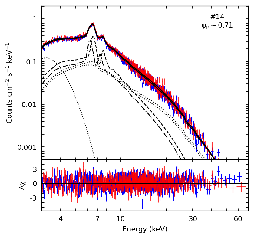
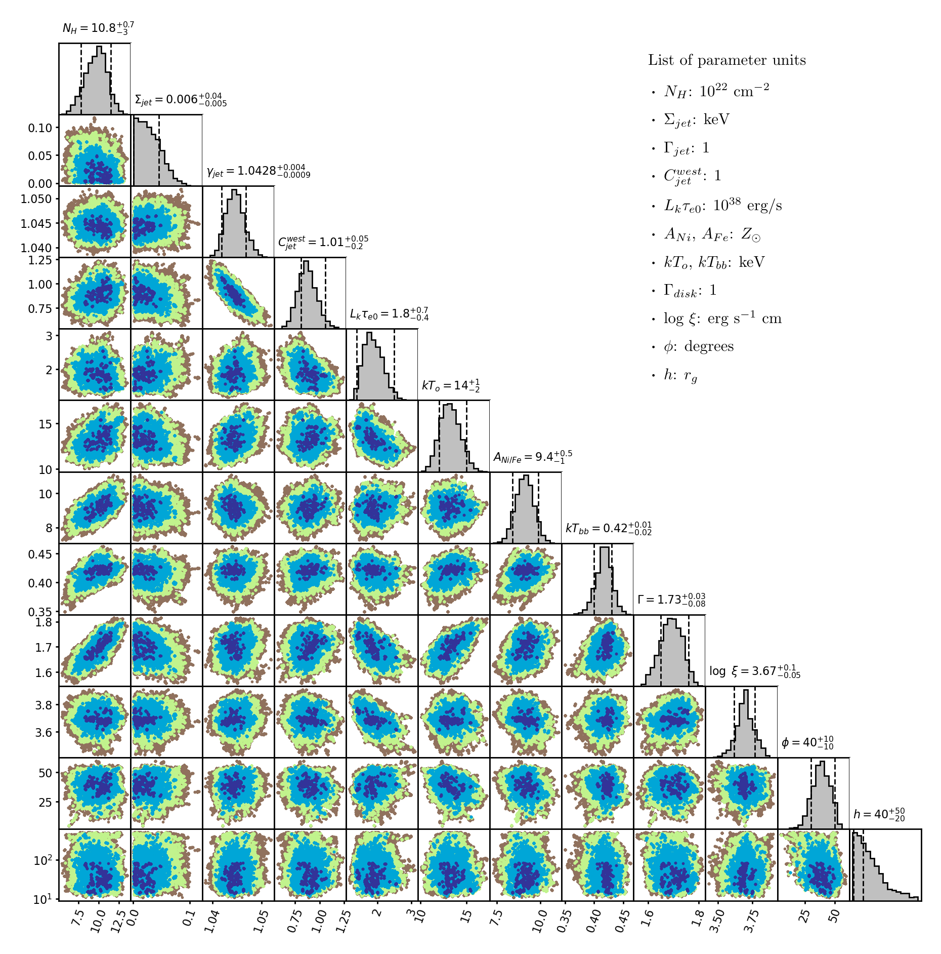
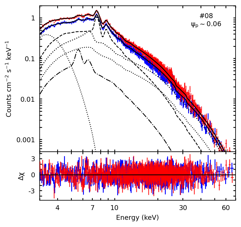
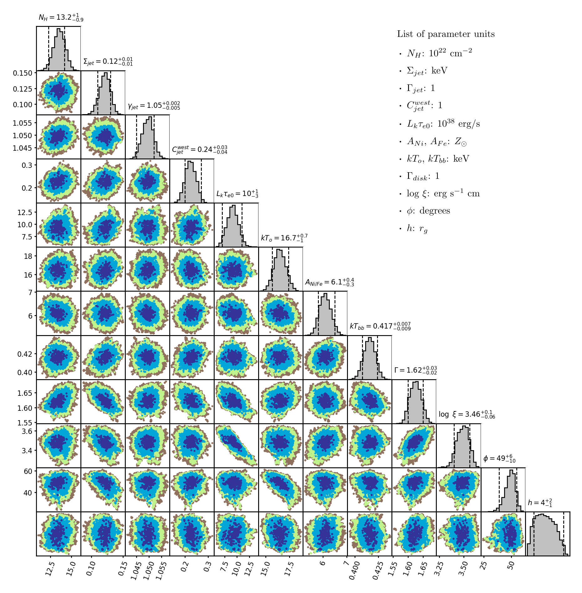
Figure 1: Left column: Sample of NuSTAR FPMA/B averaged spectra fitted with a combination of bjet, diskbb, xillverCp and relxilllpCp. Dashed line corresponds to the eastern jet model component. Dot-dashed line corresponds to the western jet model component. Dotted lines corresponds to the different disk model components. Right column: one and two dimensional distribution of some continuum model parameters derived from the MCMC simulations. Outwards colour gradient indicate confidence levels: 90%, 99%, 99.9% and 99.99%

. See Table 2 for details on parameters units.

3.2 Broadband description

On the left panels of Figure 1 we show observations #14 ($\psi_{\rm pre}\sim 0.71$) and #08 ($\psi_{\rm pre}\sim 0.06$) spectra and their best fits along with their residuals. These two examples show two very different instances of the precessional motion. Observation #14 has both jets at similar Doppler shifts and thus showing overlapping emission lines (unresolvable by NuSTAR). Observation #08 has the eastern and western jet at opposing Doppler shifts, and thus showing iron and nickel emission lines perfectly resolvable by NuSTAR (dashed and dot-dashed lines). We also clearly see the different disk component contribution (dotted lines) at very soft energies (E$<5$ keV; diskbb), the Fe K$\alpha$ line ($\sim$6.4 keV; xillverCp) and the harder (E¿20 keV) reflected component (both xillverCp and relxilllpCp).

The soft energy range of the NuSTAR spectra (E$<10$ keV) is dominated by the contribution of one or both jets and the thermal disk component. On highly blue-shifted phases ($\psi_{\rm pre}<$0.2 and $\psi_{\rm pre}$¿0.8), the western jet contribution to the total flux seems to be $\sim$0.1–0.3 times that of the eastern jet, as modelled by the attenuation factor. During the in between phases, when the merging of emission lines starts to occurs, the western jet contributes significantly more, with factors ranging from 0.6 to 1.

The absorption column density does not seem to vary significantly among the different precessional phases. It stays somewhat high and constant at an average value of $12\times 10^{22}$ cm^-2. We must note that NuSTAR lower energy detection limit of 3 keV does not allow to better constrain this parameter. Furthermore, the black body component also dominates at very low energies, so the absorption column and black body parameters (temperature and normalization) are tightly correlated (see the left panel of Figure 3).

Using the thermal diskbb component we get an inner temperature than ranges from approximately 0.36 to 0.42 keV. This model normalization $N_{\rm\texttt{diskbb}}$ can be used to estimate the inner disk radius $N_{\rm\texttt{diskbb}}=(f_{c}\leavevmode\nobreak\ R_{\rm\texttt{diskbb}}/d_{10})^{2}\leavevmode\nobreak\ \cos\phi$, where $f_{c}=1.7$ is the color-temperature correction factor (Kubota et al., 1998), and $\phi$ is the angle between the normal to the disk and the line of sight. As shown on the bottom left panel of Figure 3, we see that this parameter remains very well constrained between $1-5\times 10^{7}$ cm (10–60 $r_{g}$ for $M_{BH}=3\leavevmode\nobreak\ M_{\odot}$).

As already mentioned on the previous section, the bjet model normalization can be expressed in terms of $L_{k}$ and $\tau_{e0}$ by fixing a distance to the source. We constrain the value of $L_{k}*\tau_{e0}$ and use it as a measure of the jet kinetic power (Khabibullin et al., 2016) transverse to the outflow axis. We report the best bjet parameters on the right panel of Figure 2.. The jet kinetic luminosity ranges between $1-10$ times the Eddington luminosity ($\sim$10³⁸ erg s^-1), with higher values at extreme precessional phases. The temperature at the base of the jet (where it becomes visible in X-rays) ranges from 12 to 18 keV (within errors), averaging $\sim$15 keV. The base electron optical depth ranges between $\sim$0.1 and its maximum accesible value of 0.5.

We notice the nickel overabundance with respect to iron already reported on Medvedev et al. (2018). The nickel to iron abundance ratio varies between 5–15, being highest on the intermediate phases. Although an apparent precessional motion of this ratio can be seen (bottom right panel of Figure 2), it can be thought to be constant at $\sim$9 within 1$\sigma$.

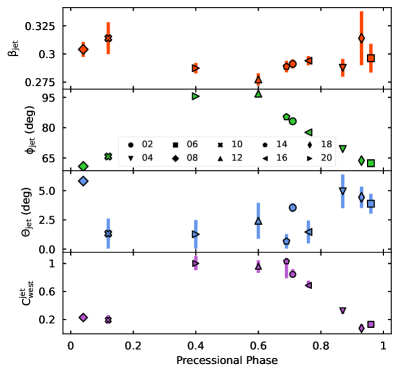
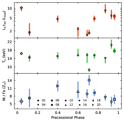
Figure 2: Precessional evolution of bjet and system parameters derived from the 3–70 keV fit to NuSTAR spectra. Left panel, top to bottom: bulk velocity factor $\beta=v/c$, jet inclination angle $\phi$, jet opening angle $\Theta$, western jet attenuation factor. Right panel, top to bottom: jet kinetic luminosity weighted by opacity $L_{k}\times\tau_{e0}$ ($10^{38}$ erg s^-1), jet base temperature $T_{o}$ and ratio of nickel to iron abundances.

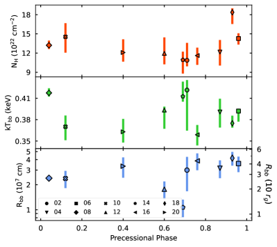
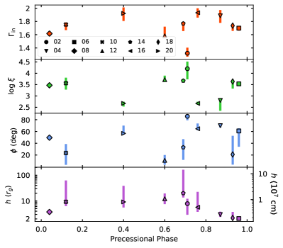
Figure 3: Precessional evolution of different disk components parameters. Left panel, top to bottom: local absorption column, diskbbinner radius temperature and inner radius. Right panel, top to bottom: incident spectral index, ionization degree, inclination angle and source height.

The disk continuum parameters show a more intricate behaviour. The incident power-law index ranges between 1.6 to 2, taking the lowest value of $\sim$1.4 at observation #02. It becomes harder towards intermediate phases, pointing to a weaker jet dominated state. It is interesting to note that the spectral index of the pexmon component used by Middleton et al. (2021) to fit the average spectra, which was tied across all 8 observations, is considerably harder than the one found in the fits to the covariance spectrum ($\sim$1.4 and $\sim$2.2 respectively). Our results lie between these two boundaries, which shows that our precessional analysis is compatible with the fits to the time-resolved covariance spectra.

Both ionization degree $\xi$ and inclination angle $\phi$ do not seem to follow any particular precessional behaviour, but instead seem somehow anti-correlated. At lower inclination angles, the ionization degree increases. This may indicate that at lower (higher) inclinations we see more (less) of the inner and hotter regions of the accretion disk, and thus reflected on a higher (lower) ionization degree of the reflecting material.

Lastly, the illuminating source height $h$ ranges (within errors) between $0.2-9\times 10^{7}$ cm (3–100 $r_{g}$ for $M_{BH}=3M_{\odot}$), taking lower values (with lower relative errors) towards extreme phases. This effect might be related to the fact that the more edge-on the accretion disk is seen, the weaker is the contribution to total flux from reflection, and thus, the most important is the contribution of direct emission. This makes the height parameter more difficult to constrain.

On the right column of Figure 1 we present the triangle plot of observations #14 and #08, where the diagonal subplots represent the one dimensional distribution (histogram) of each parameter derived from the MCMC chains. The remaining subplots contain the two dimensional distribution of values of the $i$-th column parameter with the $j$-th row parameter. Colours indicate different confidence levels: 90% (red), 99% (green) and 99.9% (blue). For better display, we show only a subset of parameters. The top label above each parameter histogram indicates the relevant parameter name and its best fit value with the 90% confidence level error range. We also included a table of units for clarity.

3.3 Flux evolution and hardness

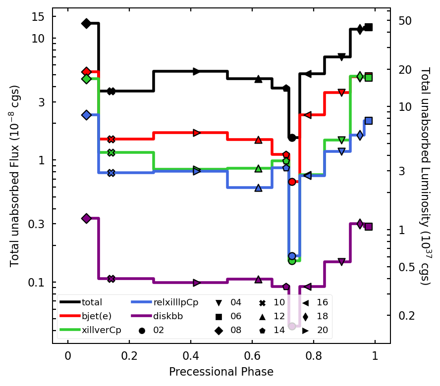
Figure 4: Spectral behaviour of the jet and disk model components. Left panel: precessional evolution of the total flux (3–70 keV) of each model component. Right panel: hardness-intensity diagram (soft: 3–10 keV, hard: 10–70 keV). The diskbb (purple) component was only included on the left panel. Error bars appear smaller than the marker size on almost all data points.

To further investigate the spectral contributions of the jet and the accretion disk along the precessional motion, we calculated each model unabsorbed flux (using cflux convolution model in XSPEC) in 2 different bands: soft: 3–10 keV and hard: 10–70 keV.

On the left panel of Figure 4 we show the precessional evolution of both defined bands for each model component. We only show the ”eastern” bjet component, as the remaining ”western” would be the same multiplied by the attenuation factor. We also show the total flux for reference.

The eastern jet component dominates and contributes from 30% up to 65% of the total observed flux depending on the precessional phase. The thermal disk component contributes $\sim$2% almost independently of phase to the total flux.

On intermediate phases, where the total flux is reduced by a third, the contribution of both jet dominates, while the contribution of the disk comes almost equally from xillverCp and relxilllpCp components. On this phase (0.15–0.85) the disk components contribute up to 30% of the total flux.

On the extreme phases, the total flux is distributed as follows: 65% from the disk (considering the 3 components) and 45% from both jet (mainly the eastern jet). Moreover, the neutral reflection component has almost the same flux as the eastern jet component. This could be attributed in part to the beaming effect produced by the particular orientation of the system on these phases.

Lastly, we note a similar precessional behaviour between the jet and disk measured fluxes, the attenuation factor and the illuminating source height. The more edge-on the accretion disk is, the less contribution to total flux from reflection there is, and thus, the more important is the contribution of the direct emission. On these precessional phases, the western jet emission becomes significant also.

When looking at the spectral distribution within energy bands on the right panel of Figure 4, we see a clear difference between systems. By defining the hardness as the ratio between the measured fluxes of 10–70 keV (hard) to 3–10 keV (soft), we see that the jet component is purely soft X-ray dominated, while the disk components (without the thermal diskbb) is purely hard X-ray dominated. We also note that as total flux increases, every component tends to a hardness ratio of 1. Inversely, as total flux decreases, the jet becomes softer and the disk harder.

As a final remark, we note that the total bjet unabsorbed luminosity on the 3–70 keV band (assuming a distance of 5.5 kpc), ranges from $0.2-2\times 10^{38}$ erg s^-1. These values are approximately 2 to 10 times that of the measured kinetic luminosities (see Figure 2). On the intermediate phases, the ratio between these two kind of luminosities is the greatest.

4 Discussion

4.1 Precessing lines and kinematic model

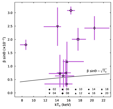
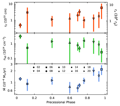
Figure 5: Left: Relationship between the temperature at the base of the jet and the transversal velocity of matter throught the jet. We plot the expected velocity caused by adiabatic expansion of the jet. Right: Precessional evolution of different jet parameters (see text for equations). From top to bottom: jet base height from cone apex, electron density at base height and mass flow rate through the jet.

From the obtained values of both jet redshifts $Z$ and the broadening factor of the lines $\Sigma$, we use the kinematic model equations in order to compute the bulk velocity of matter across the jet, $\beta_{\rm jet}=v/c$, the angle sustained by the eastern jet with respect to the observer $\phi$, and the half opening angle $\Theta$ of the jet.

Let us define $z_{e}$ and $z_{w}$ as the respective eastern and western jet redshifts. Then, by assuming perfect alignment between jets and equal velocities, we have:

$$\beta=\sqrt{1-\frac{1}{(1+z_{o})^{2}}}\leavevmode\nobreak\ {\rm with}\leavevmode\nobreak\ z_{o}=\frac{z_{e}+z_{w}}{2}.$$ (1)

By application of kinematic equations (see Cherepashchuk et al., 2018 for full set of equations) we can express the angle between the jet axes and the line of sight in terms of both jet redshifts:

$$\cos\leavevmode\nobreak\ \phi=\frac{z_{w}-z_{e}}{2\gamma\beta}\leavevmode\nobreak\ {\rm with}\leavevmode\nobreak\ \gamma=1+z_{o}\leavevmode\nobreak\ \rm{the\leavevmode\nobreak\ Lorentz\leavevmode\nobreak\ factor.}$$ (2)

Lastly, by considering the line profiles to be Gaussians with dispersion $\Sigma$ ($E_{o}$) (with $E_{o}$ the line centroid at rest) we can estimate the jet half opening angle (Marshall et al., 2002):

$$\Theta=\sqrt{\frac{2\leavevmode\nobreak\ \log\leavevmode\nobreak\ 2}{3}}\leavevmode\nobreak\ \frac{2}{\gamma\leavevmode\nobreak\ \beta\leavevmode\nobreak\ \sin\phi}\leavevmode\nobreak\ \frac{\Sigma(E_{o})}{E_{o}}.$$ (3)

The application of these three equations can be seen on the left panel of Figure 2.

Overall, we get an average bulk velocity factor $\beta\sim 0.29$, and with values (and errors) that increase towards extreme phases. This effect comes from the fact that at higher redshift, the western jet redshift becomes harder to constrain, as its flux becomes significantly lower than the eastern jet, and competes with the thermal diskbband the reflection components. For comparison, the reference value obtained from decades of optical data is of $\sim 0.26$ (Cherepashchuk et al., 2018).

From the inclination angle we can derive estimates to the mean inclination of the system and the precession angle that the jet sustain with respect to the axis of rotation. By fitting a linear function to the second half of precessional phases ($>$0.5), we get an inclination of approximately 82 degrees and a precession angle of $\sim$23 degrees which are in complete agreement with the ephemeris of Eikenberry et al. (2001).

The half opening angle of the jet can range between 1 up to 6 degrees, with lower values (but greater relative errors) on intermediate phases (0.15–0.85). This comes from the fact that on these phases the width of the emission lines becomes harder to constrain as they start to overlap, and with NuSTAR’s resolution they cannot be resolved separately.

An interesting result comes from comparing the expansion velocity of the jet perpendicular to the jet axis ($\beta$ $\sin\Theta$), and the sound speed in the rest frame of the flowing gas

$$\beta_{s}=v_{s}/c=\sqrt{\frac{5kT_{o}}{3\mu(1+X)m_{p}c^{2}}},$$ (4)

where $kT_{o}$ is the measured temperature of the gas at the base of the jet, m_p is the proton mass, $\mu\sim 0.62$ the mean molecular weight and $X=n_{i}/n_{e}\sim 0.91$ the ion to electron ratio. We show this relationship on the left panel of Figure 5. We note that within errors, the relationship between these parameters holds true for small angles where $\sin\Theta\sim\Theta$. By looking at Figure 2, we see that this corresponds to observations on intermediate phases (0.15–0.85) where $\Theta<2$ degrees. As suggested by Marshall et al. (2002) this relationship might be physical, interpreted as the jet expanding sideways at the sound speed of plasma at its base.

4.2 Outflow overview

By following Khabibullin et al. (2016), we can estimate the evolution of some of the initial conditions at the base of the jet, using the derived fit parameters. Namely, the height from the jet cone apex where it becomes visible to an observer:

$$r_{o}\sim 1.2\times 10^{6}\leavevmode\nobreak\ \mathrm{cm}\times{L_{k}}/(\tau_{e0}\beta^{3}\Theta),$$ (5)

and the electron density at this radius:

$$n_{e0}\sim 1.25\times 10^{18}\leavevmode\nobreak\ \mathrm{cm}^{-3}\times\tau_{e0}^{2}\beta^{3}/{L_{k}}.$$ (6)

As shown in the right panel of Figure 5, we see that the jet base (also referred as truncation radius) is of the order of 10¹⁰ cm ($\sim$1.1$\times$10⁴ $r_{g}$ for $M_{BH}=3M_{\odot}$), ranging from 0.5 to 5 times this value. By taking averaged values of $\Theta$ and $r_{o}$ we can estimate the size of the jet base $r_{o}\Theta\sim 5.2\times 10^{8}$cm ($\sim$600 $r_{g}$).

The electron density at the jet base $n_{e0}$ ranges from 0.2 to $4\times 10^{14}$ cm^-3. We note that these two quantities follow a simplified version of the continuity equation, with $n_{e0}r_{o}^{2}\sim 4\times 10^{34}\leavevmode\nobreak\ cm^{-1}$ remaining constant throughout the jet.

Finally, we can estimate the mass flow through the jet by combining all the above quantities:

$$\dot{M}=\mu m_{p}(1+X)n_{e0}\pi r_{o}^{2}\Theta^{2}\beta c.$$ (7)

We show this result on the right–bottom panel of Figure 5. We see that the mass flow rate ranges between 0.4 up to $3\times 10^{-6}$ M_⊙ yr^-1. Assuming a mass of 3 $M_{\odot}$ for the compact object (Cherepashchuk et al., 2018), we get a maximum of $\sim$20 times the Eddington mass transfer rate.

For reference, Marshall et al. (2002) obtain a value $r_{o}\sim\leavevmode\nobreak\ 2\times 10^{10}\leavevmode\nobreak\$cm which lies very well between our estimates. Conversely, they obtain a higher upper limit of $4\times 10^{15}$ cm^-3 for the electron density at the jet base, almost ten times our upper limit. This gives $n_{e0}r_{o}^{2}\sim 1.7\times 10^{36}$ cm^-1, $\lesssim$100 times greater than our estimate.

By taking the maximum measured 3–70 keV bjet luminosity ($2\times 10^{38}$ erg s^-1), we can compute the photoionization degree $\xi$ over the spherical region of size $r_{o}$ and electron density $n_{e0}$, $\log\leavevmode\nobreak\ \xi=\log\leavevmode\nobreak\ L_{x}$/($n_{e0}r_{o}^{2})\lesssim 4$. This means that the illuminating jet power is sufficient to account for the higher ionization degrees obtained by the reflection components. As already stated by Middleton et al. (2021), the use of more complex reflection models, such as xillverCp and relxilllpCp, provides a more detailed description of the reflecting medium.

The high absorption column obtained in the spectral fits could be associated with a region of the wind around the jets, which separates the visible part from the invisible one. The density of this region provides an appreciable optical depth for photo-absorption, blocking the jet and thermal disk emission at energies below $\sim$10 keV, but, at the same time, being optically thin for electron scattering; thus partially scattering photons with higher energies.

This concept has already been developed by Medvedev et al. (2018) (cwind model), and they estimate that such condition would require an absorbing column density $N_{H}$ between $15-20\times 10^{22}$ cm^-2 with on optical depth of the order of 0.1. These estimates are in fully in agreement with our obtained values of both parameters.

We can estimate the size of this region if we assume that $n_{e0}R\propto N_{H}$, ie, a balance between neutral hydrogen and free electrons. By taking average values of $N_{H}$ and $n_{e0}$ we get $R\sim 1.5\times 10^{9}$ cm ($\sim$1700 $r_{g}$ for $M_{BH}=3M_{\odot}$), which is very similar (within errors and approximations) to the accretion disk spherization radius $R_{sph}\sim 1.8\times 10^{9}$ cm$\sim 2000\leavevmode\nobreak\ r_{g}$ where the accretion regime becomes supercritical (Medvedev et al., 2018). This suggests that the absorbing region originates from the combined effect of the high accretion rate, which generates dense gas structures around the compact object in SS 433, and the supercritical disk winds which effectively scatter the soft ($E<10$ keV) photons.

Middleton et al. (2021) attribute the disk wind cone (Dauser, Middleton, & Wilms, 2017) as responsible for the lags found at energies up to 9 keV and the hard x-ray excess at 20–30 keV. We frame these results in our scenario by linking the disk wind cone with the combined effect of the reflected spectrum and the central obscuring region.

Specifically, the wind cone model assumes low opening angles ($<10$ degrees) for velocities $\beta\sim$0.2–0.4 to show beaming effects, and a cone height of $10^{5}\leavevmode\nobreak\ r_{g}\sim 9\times 10^{10}$ cm. Both these model assumptions are in agreement with the values that we found ($\beta\sim$0.28–0.32 and $r_{o}<10^{11}\leavevmode\nobreak\$cm).

According to our fitting results, we attribute the reflected spectrum of the accretion disk as responsible for the hard excess component (see Figure 4), and make the case for this obscuring region as the wind itself reprocessing Fe XXV and Fe XXVI emission lines (6.7 and 6.97 keV respectively) and thus shifting them onto higher energies. For this to be possible we followed calculations by Inoue (2022), who estimated an optical depth of $\sim$1.6 for a compact object of 10 M_BH and a radius of 10¹² cm. If we re-scale by the magnitudes used and obtained in our paper, we find that a lower optical depth of $\tau>0.02$ is sufficient to account for soft-photon scattering. We find optical depths at the jet base $\tau_{e0}>0.1$ that satisfy the former condition.

5 Conclusions

We have reported on the analysis of 10 NuSTAR observations of the Galactic microquasar SS433 that span 1.5 precessional cycles which were taken on almost the same orbital phase. We model the averaged spectra with a combination of two precessing thermal jet (bjet; Khabibullin et al. (2016)) and cold (xillverCp; García et al. (2013)) and relativistic reflection (xillverCp; Dauser et al. (2014)) emission from an black body type accretion disk (diskbb). We also included Doppler shifting (zashift) and broadening (gsmooth) components, as well as local and Galactic absorption (tbabs).

Our main results are summarised as follows:

1. Jet bulk velocity ranges between 0.28–0.32$c$ and the jet half opening angle is $\lesssim$6 degrees.

2. The bjet kinetic luminosity ranges between $2-20\times 10^{38}$ erg s^-1, with an average base temperature of $\sim$16 keV and a nickel to iron ratio of $\sim$9.

3. The western jet relative flux with respect to the eastern jet flux ranges from 0.2 on extreme phases up to $\sim$1 on intermediate phases.

4. The diskbb component gives an inner disk temperature of $\sim$0.38 keV with an inner radius of $\lesssim$30 $r_{g}$.

5. The total 3–70 keV luminosity of both jet and disk reflection components range between $0.2-2\times 10^{38}$ erg s^-1, with the jet being completely soft X-ray dominated (3–10 keV), and the disk reflection components hard X-ray dominated (10–70 keV).

6. We find that at low half opening angles ($\lesssim 2^{\circ}$), the jet sideways velocity, $\beta\sin\Theta$, can be expressed in terms of the jet base temperature, indicating that it follows an adiabatic expansion regime.

7. The unabsorbed jet luminosity $L_{x}\lesssim 2\times 10^{38}$ erg s^-1 is sufficient to account for the high ionization degrees (log $\xi\lesssim$4) obtained from the reflection components.

8. The central source and lower parts of the jets could be hidden by an optically thick region of $\tau>0.1$ and size $R\sim N_{H}/n_{e0}\sim 1.5\times 10^{9}$ cm$\sim 1700$ $r_{g}$ for $M_{BH}=3\leavevmode\nobreak\ M_{\odot}$.

Appendix A

On Table 2 we present the complete best-fit parameters with errors reported to 90% confidence level, extracted from MCMC chains of 7$\times$10⁶ steps (after burning-in the same amount), obtained using 360 walkers (20 times the number of free parameters).

To check for MCMC convergence, we visually inspected the chains of each parameter and determined the most appropriate number of burn-in steps in order to obtain uncorrelated series for the parameters of interest. We corroborated this method by computing the integrated autocorrelation time associated with each series, and verified that it remained as close as unity as possible.

We show an example of a chain ’trace’ plot which converged on Figure 6. The integrated autocorrelation time $\tau$ is very close to unity, which serves as an numerical indicator of the chain convergence.

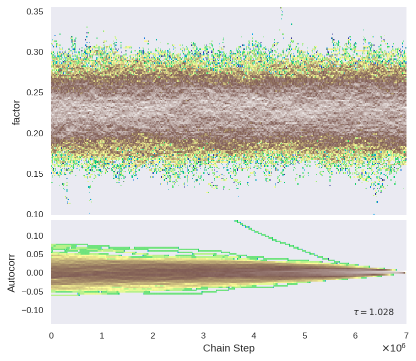
Figure 6: Example of ’trace’ plot derived from a MCMC chain. The integrated autocorrelation time $\tau$ is close to unity, which serves as an indicator of the chain convergence. Color gradient indicates density of data points.

constant $\times$ tbabs $\times$ tbabs $\times$ ( zashift $\times$ bjet + constant $\times$ zashift $\times$ bjet + diskbb + xillverCp + relxilllpCp)
Obs	$N_{H}$	$\Sigma^{\rm jet}_{\rm 6keV}$	$Z^{\rm jet}_{\rm east}$	$L_{38}$ * $\tau_{e0}$	$T_{o}$	$A^{\rm jet}_{\rm Fe}$	$A^{\rm jet}_{\rm Ni}$	$C^{\rm jet}_{\rm west}$	$Z^{\rm jet}_{\rm west}$
02	$8^{+4}_{-2}$	$0.03^{+0.06}_{-0.003}$	$0.008^{+0.003}_{-0.0008}$	$10^{+4}_{-1}$	$11^{+0.9}_{-1}$	$1.1^{+0.1}_{-0.2}$	$14^{+2}_{-0.9}$	$0.92^{+0.08}_{-0.06}$	$0.081^{+0.005}_{-0.001}$
04	$12^{+1}_{-2}$	$0.09^{+0.03}_{-0.01}$	$-0.062^{+0.002}_{-0.001}$	$25^{+7}_{-1}$	$14^{+0.5}_{-2}$	$1.2^{+0.02}_{-0.1}$	$9^{+0.9}_{-1}$	$0.32^{+0.02}_{-0.04}$	$0.15^{+0.004}_{-0.005}$
06	$14^{+0.7}_{-1}$	$0.08^{+0.02}_{-0.02}$	$-0.097^{+0.001}_{-0.0005}$	$30^{+10}_{-2}$	$18^{+1}_{-0.9}$	$2.2^{+0.3}_{-0.5}$	$15^{+2}_{-3}$	$0.12^{+0.03}_{-0.03}$	$0.19^{+0.007}_{-0.01}$
08	$13.2^{+0.7}_{-0.5}$	$0.124^{+0.007}_{-0.005}$	$-0.1059^{+0.0006}_{-0.0005}$	$21^{+3}_{-2}$	$16.4^{+0.7}_{-0.6}$	$2.2^{+0.3}_{-0.3}$	$13^{+2}_{-2}$	$0.23^{+0.02}_{-0.02}$	$0.205^{+0.004}_{-0.005}$
10	$15^{+2}_{-2}$	$0^{+0.05}_{-0.002}$	$-0.083^{+0.001}_{-0.001}$	$14^{+8}_{-2}$	$15^{+1}_{-2}$	$2.4^{+0.3}_{-0.9}$	$17^{+3}_{-8}$	$0.19^{+0.06}_{-0.05}$	$0.19^{+0.01}_{-0.008}$
12	$14^{+2}_{-3}$	$0.05^{+0.02}_{-0.04}$	$0.073^{+0.005}_{-0.002}$	$8^{+3}_{-0.4}$	$18^{+3}_{-3}$	$2.6^{+0.3}_{-0.6}$	$29^{+1}_{-6}$	$0.9^{+0.1}_{-0.05}$	$0.006^{+0.003}_{-0.001}$
14	$11^{+1}_{-3}$	$0^{+0.04}_{-0.0005}$	$0.02^{+0.002}_{-0.002}$	$11^{+3}_{-1}$	$13^{+2}_{-1}$	$2.4^{+0.4}_{-0.3}$	$21^{+3}_{-2}$	$0.9^{+0.1}_{-0.1}$	$0.068^{+0.004}_{-0.001}$
16	$12^{+1}_{-1}$	$0.04^{+0.02}_{-0.03}$	$-0.019^{+0.001}_{-0.002}$	$17^{+3}_{-2}$	$16^{+0.8}_{-1}$	$1.3^{+0.08}_{-0.1}$	$12^{+1}_{-1}$	$0.69^{+0.07}_{-0.04}$	$0.112^{+0.002}_{-0.003}$
18	$18^{+1}_{-0.8}$	$0.1^{+0.02}_{-0.01}$	$-0.093^{+0.0005}_{-0.001}$	$27^{+4}_{-5}$	$22^{+0.9}_{-3}$	$2.3^{+0.3}_{-0.3}$	$13^{+2}_{-2}$	$0.08^{+0.04}_{-0.03}$	$0.2^{+0.009}_{-0.02}$
20	$13^{+1}_{-2}$	$0.01^{+0.04}_{-0.007}$	$0.073^{+0.003}_{-0.001}$	$17^{+2}_{-3}$	$15^{+2}_{-1}$	$1.1^{+0.2}_{-0.08}$	$13^{+1}_{-0.8}$	$0.98^{+0.09}_{-0.08}$	$0.015^{+0.002}_{-0.001}$
Obs	$kT_{bb}$	$N_{bb}$	$\Gamma_{in}$	$\log\leavevmode\nobreak\ \xi$	$\phi$	$N_{\rm xi}$	$h$	$C_{AB}$	$\chi^{2}$ / dof
02	$0.45^{+0.05}_{-0.05}$	$0.02^{+0.1}_{-0.02}$	$1.4^{+0.1}_{-0.07}$	$2.7^{+0.07}_{-0.2}$	$82^{+2}_{-5}$	$1.2^{+0.2}_{-0.4}$	$20^{+70}_{-10}$	$1.01^{+0.02}_{-0.004}$	669.52/642
04	$0.39^{+0.01}_{-0.01}$	$1.2^{+0.6}_{-0.4}$	$1.9^{+0.04}_{-0.1}$	$2.8^{+0.04}_{-0.2}$	$70^{+2}_{-3}$	$9^{+1}_{-2}$	$2.9^{+0.8}_{-0.5}$	$1.024^{+0.006}_{-0.005}$	1137.00/1016
06	$0.39^{+0.003}_{-0.02}$	$2.6^{+0.8}_{-0.4}$	$1.71^{+0.02}_{-0.04}$	$3.6^{+0.05}_{-0.1}$	$60^{+6}_{-10}$	$12^{+2}_{-2}$	$2.2^{+0.5}_{-0.2}$	$1.035^{+0.004}_{-0.005}$	1448.34/1333
08	$0.418^{+0.007}_{-0.004}$	$1.3^{+0.2}_{-0.1}$	$1.62^{+0.02}_{-0.02}$	$3.47^{+0.07}_{-0.07}$	$50^{+4}_{-4}$	$8.3^{+0.6}_{-0.9}$	$3.7^{+0.6}_{-0.7}$	$1.047^{+0.003}_{-0.003}$	1405.17/1340
10	$0.37^{+0.01}_{-0.02}$	$1.8^{+0.8}_{-0.6}$	$1.75^{+0.03}_{-0.05}$	$3.6^{+0.1}_{-0.2}$	$20^{+20}_{-20}$	$1.8^{+0.2}_{-0.5}$	$10^{+20}_{-3}$	$1.01^{+0.01}_{-0.009}$	686.64/674
12	$0.38^{+0.02}_{-0.009}$	$1.4^{+0.6}_{-0.7}$	$1.7^{+0.06}_{-0.09}$	$3.8^{+0.1}_{-0.2}$	$10^{+10}_{-8}$	$1.7^{+0.3}_{-0.2}$	$9^{+5}_{-2}$	$1.042^{+0.007}_{-0.007}$	851.57/894
14	$0.42^{+0.01}_{-0.03}$	$0.3^{+0.1}_{-0.1}$	$1.7^{+0.05}_{-0.06}$	$3.7^{+0.1}_{-0.1}$	$40^{+6}_{-20}$	$1.4^{+0.2}_{-0.3}$	$20^{+40}_{-10}$	$1.03^{+0.003}_{-0.01}$	903.51/864
16	$0.36^{+0.01}_{-0.01}$	$1.8^{+0.7}_{-0.6}$	$1.93^{+0.04}_{-0.07}$	$2.67^{+0.07}_{-0.05}$	$65^{+3}_{-2}$	$4^{+1}_{-0.6}$	$6^{+4}_{-2}$	$1.055^{+0.006}_{-0.005}$	989.56/987
18	$0.38^{+0.006}_{-0.01}$	$5^{+2}_{-0.8}$	$1.74^{+0.02}_{-0.04}$	$3.6^{+0.04}_{-0.1}$	$20^{+30}_{-8}$	$9^{+2}_{-0.9}$	$2^{+2}_{-0.1}$	$1.022^{+0.005}_{-0.004}$	1383.68/1301
20	$0.36^{+0.02}_{-0.01}$	$1.9^{+0.6}_{-0.8}$	$1.91^{+0.09}_{-0.04}$	$2.7^{+0.04}_{-0.1}$	$60^{+6}_{-6}$	$4^{+1}_{-0.6}$	$10^{+20}_{-7}$	$1.015^{+0.004}_{-0.007}$	944.15/929

Table 2: Complete model best fit parameters and fit statistics.

$N_{H}$ : local absorption column density in 10²² cm^-2 units.

$\Sigma^{\rm jet}_{\rm 6keV}$ : Gaussian smoothing factor at $E=6$ keV in eV units.

$Z^{\rm jet}_{\rm east}$, $Z^{\rm jet}_{\rm west}$ : eastern and western jet redshifts.

$C^{\rm jet}_{\rm west}$ : western jet attenuation factor.

$L_{38}$ * $\tau_{e0}$ : jet kinetic luminosity weighted by electron transverse opacity in 10³⁸ erg/s units .

$T_{o}$ : jet base temperature in keV units.

$A^{\rm jet}_{\rm Fe}$, $A^{\rm jet}_{\rm Ni}$ : jet iron and nickel abundances in solar units.

$kT_{\rm bb}$ : diskbb temperature in keV units.

$N_{\rm bb}$ : diskbb normalization ($\times$10⁴).

$\Gamma_{in}$ : xillverCp incident powerlaw index.

$\log\leavevmode\nobreak\ \xi$ : xillverCp ionization degree.

$\phi$ : xillverCp inclination angle in degree units.

$h$ : relxilllpCp illuminating source height in gravitational radii units.

$N_{\rm xi}$ : xillverCp (equal to relxilllpCp) normalization ($\times$10^-4).

$C_{AB}$ : FPMA/B cross correlation factor.

On Figure 7 we present a schematic picture of the microquasar SS433, where the X-ray emission from the jets and the accretion disk components of our scenario are depicted. We also indicate the different geometrical parameters involved, together with specific physical parameters of the model.

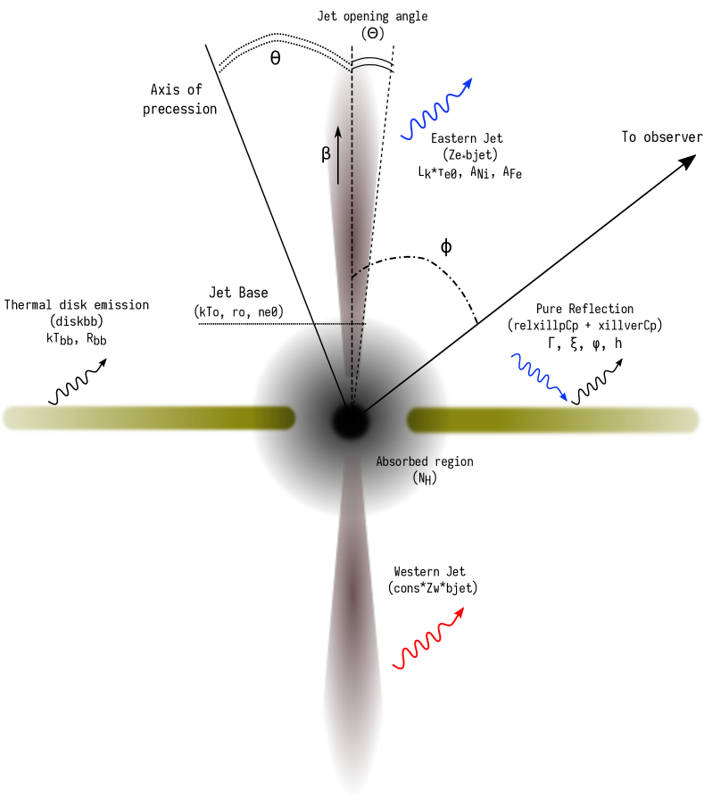
Figure 7: Schematic view of SS433. Each model component is indicated, with the most relevant parameters of the system.