The Gauge Picture of Quantum Dynamics
Abstract
Although local Hamiltonians exhibit local time dynamics, this locality is not explicit in the Schrödinger picture in the sense that the wavefunction amplitudes do not obey a local equation of motion. We show that geometric locality can be achieved explicitly in the equations of motion by “gauging” the global unitary invariance of quantum mechanics into a local gauge invariance. That is, expectation values are invariant under a global unitary transformation acting on the wavefunction and operators , and we show that it is possible to gauge this global invariance into a local gauge invariance. To do this, we replace the wavefunction with a collection of local wavefunctions , one for each patch of space . The collection of spatial patches is chosen to cover the space; e.g. we could choose the patches to be single qubits or nearest-neighbor sites on a lattice. Local wavefunctions associated with neighboring pairs of spatial patches and are related to each other by dynamical unitary transformations . The local wavefunctions are local in the sense that their dynamics are local. That is, the equations of motion for the local wavefunctions and connections are explicitly local in space and only depend on nearby Hamiltonian terms. (The local wavefunctions are many-body wavefunctions and have the same Hilbert space dimension as the usual wavefunction.) We call this picture of quantum dynamics the gauge picture since it exhibits a local gauge invariance. The local dynamics of a single spatial patch is related to the interaction picture, where the interaction Hamiltonian consists of only nearby Hamiltonian terms. We can also generalize the explicit locality to include locality in local charge and energy densities.
I Introduction
Locality is of fundamental importance in theoretical physics. The observable physics of quantum dynamics is local if the Hamiltonian is geometrically local111Geometric locality is not to be confused with the weaker notion of -locality, for which an operator is -local if it acts on at most qubits anywhere in space., i.e. if the Hamiltonian is a sum of local operators. An operator (other than the Hamiltonian) is said to be local if it only acts on a small region of space. But locality is not explicit in the Schrödinger picture because the wavefunction is global in the sense that it can not be associated with any local region of space, and the time dynamics of the wavefunction globally depends on all Hamiltonian terms. On the other hand, locality is explicit in the Heisenberg picture, for which the time dynamics of local operators only depends on nearby local operators (when the Hamiltonian is local). Deutsch and Hayden (2000) This motivates us to ask: Is it possible to modify the Schrödinger picture to make locality explicit in the equations of motion?
Gauge theory is another fundamental concept in theoretical physics. Gauge theory is the foundation of the Standard Model of particle physics and is also used to describe exotic phases of condensed matter Levin and Wen (2005); Senthil et al. (2004). An important tool that gauge theory provides is the gauging process, in which one promotes a global symmetry into a local gauge symmetry by coupling the original model to gauge fields. For example, a scalar field theory is invariant under a global symmetry . By coupling to a gauge field as in , the global symmetry is promoted to a local gauge symmetry where and . Gauging more exotic symmetries leads to more exotic physics; e.g. gauging spatial symmetries can lead to gravity and gauging fractal symmetries can result in fracton topological order Yoshida (2013). In quantum mechanics, expectation values are invariant under a global unitary transformation acting on the wavefunction and operators . Although this transformation is typically viewed as a global invariance rather than a global symmetry, we can still ask: Is it possible to gauge the global unitary invariance in quantum mechanics? And what are the consequences of doing so?
We find that the answer to both questions is yes, and that one consequence of gauging the global unitary invariance is that locality becomes explicit in the equations of motion. In order to achieve this, we introduce a collection of local wavefunctions , each associated with a local patch of space. Each local wavefunction is an element of the same Hilbert space as the usual wavefunction. The local wavefunction associated with nearby patches are related by unitary transformations , which are also dynamical. Locality is explicit in the sense that the equations of motion [Eq. (19)] for the dynamical variables ( and ) only depends on nearby Hamiltonian terms and nearby dynamical variables. (Note that locality is not explicit in Schrödinger’s picture in this way.)
The Schrödinger and Heisenberg pictures are related by a time-dependant unitary transformation that acts on the wavefunctions and operators. Our new picture of quantum dynamics is related to the Schrödinger and Heisenberg pictures via a local gauge transformation. We describe these derivations in detail in Sec. II and Sec. III. The new local equations of motion are given in Eq. (19), and the local gauge transformation is given in Eq. (22).
In Sec. IV, we show that the gauge picture local wavefunction associated with a patch is equivalent to the interaction picture wavefunction when the interaction Hamiltonian is the sum over Hamiltonian terms that have some support on that patch. To gain intuition, in Sec. V we consider the example of a quantum circuit in the gauge picture. In Sec. VI, we describe the measurement process in the gauge picture. Although local unitary dynamics are explicitly local in the gauge picture, the affect of local measurement is not explicitly local in the gauge picture (similar to the Schrödinger picture). In Sec. VII, we generalize spatial locality in the gauge picture to e.g. locality in local particle number or local energy density.
II Schrödinger to Heisenberg Picture
To warm up, we first derive the Heisenberg picture from the Schrödinger picture. In the Schrödinger picture, the wavefunction evolves according to
| (1) |
where is the Hamiltonian (and we set ). We use superscripts “S” and “H” to respectively label time-dependent variables in the Schrödinger and Heisenberg pictures.
To derive the Heisenberg picture, consider applying a time-dependent unitary transformation to the wavefunction and operators:
| (2) | ||||
Equation (2) defines the meaning of the “H” superscript for all operators and wavefunctions. This unitary transformation has the essential property that it does not affect expectation values:
| (3) |
Since does not affect the physics, the unitary transformation could therefore be viewed as a global “gauge” transformation, which we will use to move the time dynamics from the wavefunction to the operators.
Let be the Hermitian operator such that
| (4) |
Or equivalently, where is defined by Eq. (2). The time derivatives of the new wavefunction and operators are
| (5) |
where [Eq. (2)].
To obtain the Heisenberg picture, we simply choose
| (6) |
with the initial condition at , where denotes the identity operator. This choice makes the wavefunction constant in time, while operators evolve in time. If the Hamiltonian is time-independent, then the Hamiltonian is the same in the Schrödinger and Heisenberg pictures; i.e. if .
II.1 Locality
A nice feature of the Heisenberg picture is that if the Hamiltonian is local, then the time evolution of observables is explicitly local. A local Hamiltonian has the form
| (7) |
where each only acts on a finite patch of space . We use capital letters, , , and , to denote patches of space.
Now consider the time evolution of a local operator in the Heisenberg picture:
| (8) |
Throughout this work, denotes a local operator that acts within the spatial patch (when viewed in the Schrödinger picture), and similar for , etc. Due to locality, most Hamiltonian terms cancel out in the first term. The result is an explicitly local Heisenberg equation of motion:
| (9) |
where [Eq. (2)]. is a sum over nearby Hamiltonian terms:
| (10) |
denotes a sum over patches that have overlap with patch . Note that the local Hamiltonian terms also evolve according to Eq. (9).
Locality is explicit in this local Heisenberg picture because the time evolution of each local operator only depends on nearby time-dependent operators . Locality is not explicit in Schrödinger’s picture since the time evolution of the wavefunction globally depends on all Hamiltonian terms, and there is no sense in which the wavefunction (or parts of it) can be associated with a point in space.
III Gauge Picture
We now want to obtain a local picture of quantum dynamics that features time-dependent wavefunctions and time-independent operators. To do this, we first choose a set of local patches of space that cover the entire space (or lattice); see Fig. 1 for an example. Then for each patch of space, we apply a time-dependent unitary transformation to the Heisenberg picture wavefunction and local operators:
| (11) | ||||
We thus obtain a separate local wavefunction for each patch of space. For a certain transformation , the wavefunctions are local in the sense that their dynamics are local and only depend on nearby Hamiltonian terms. Note that is a many-body wavefunction that belongs to the same Hilbert space as the usual wavefunction. The second line transforms local operators (including and ) from the Heisenberg picture into a new picture of quantum dynamics. The “G” superscript labels time-dependent operators that evolve within this picture. We omit the “G” superscript for since the notation is not used in other pictures; thus, there should be no confusion. To further reduce clutter, we also suppress the “” notation for time-dependent variables.
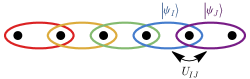
After applying this unitary transformation, correlation functions within a single patch become . Correlation functions of operator products acting on multiple patches becomes
| (12) | ||||
where we define
| (13) |
A connection always appears between variables associated with different spatial patches. Equation (11) implies that the following identities hold for all :
| (14) | ||||
and and . Therefore, serves the role of a connection that transports the local wavefunctions between different spatial patches. But the connections are trivial in the sense that there is no curvature or nontrivial holonomy (e.g. ).
Let be the Hermitian operator such that
| (15) |
Then the time derivatives of the local wavefunctions and operators are
| (16) | ||||
This follows from and Eqs. (9) and (11). is defined from Eq. (11).
A nice choice for at and is
| (17) | ||||
since this makes local operators (and Hamiltonian terms) equal to Schrödinger picture operators:
| (18) |
We thus obtain the gauge picture equations of motion, for which the local wavefunctions (which are vectors in the many-body global Hilbert space) and operators evolve as follows:
| (19) |
is defined from Eqs. (10) and (11) and can be expressed as
| (20) |
Although the Schrödinger and Heisenberg pictures are linear differential equations, the gauge picture involves non-linear differential equations for . The initial conditions are
| (21) | ||||
Note that one does not need to keep track of a for every pair of and ; only considering overlapping pairs of spatial patches suffices. If we want to describe the dynamics of a mixed state, then we could take to be a purification of the mixed state.
Thus, we were able to make Schrödinger’s picture explicitly local by introducing a local wavefunction for each patch of space and unitary connections that map between the Hilbert spaces of the different patches. Locality is explicit in the sense that the time evolution of and only depends on nearby variables (, , and ).
In the gauge picture, physical correlation functions [e.g. Eq. (12)] are invariant under the following local gauge invariance:
| (22) |
where are arbitrary unitary transformations. For example, and are not invariant under this transformation and are therefore not physical in the sense that they are not equal to or in the Heisenberg (or Schrödinger) picture. Therefore, the local wavefunctions are local in the sense that they can only be used to calculate local expectation values of local operators acting within the associated spatial patch, unless we make use of connections to connect different patches. The above gauge transformation can be used to transform the gauge picture to the Heisenberg picture (with ) by taking or to the Schrödinger picture by taking .
Note that Eq. (22) generalizes the usual global unitary invariance in quantum mechanics (where and ) to a local unitary invariance. Due to the appearance of this local gauge invariance, we call this picture of quantum dynamics the gauge picture.
In order to extract the Schrödinger picture wavefunction from the gauge picture, one can use the correlation functions to first calculate the density matrix. For example, for a system of qubits, the density matrix is
| (23) | ||||
where are Pauli operators. Here we take each patch to consist of just a single qubit so that indexes the qubits/patches along some path. If the gauge picture is initialized to a pure state using Eq. (21), then will always be pure, and the wavefunction can be uniquely obtained from (up to a phase) as the only eigenvector of with nonzero eigenvalue. More generally however, the gauge picture can encode a mixed state [as explained below Eq. (21)].
As an alternative to Eq. (19), local dynamics can also be calculated by integrating
| (24) |
[from Eq. (15)] with initial condition . Equation (24) can be rewritten more explicitly as
| (25) |
Since wavefunctions are constant in the Heisenberg picture, Eq. (11) implies that the time-evolved local wavefunction is
| (26) |
III.1 Solving the Equations of Motion
Let us derive an expression for in terms of just the Hamiltonian. Simplifying Eq. (25) using [Eq. (11)] and [Eq. (10)] yields
| (27) |
The second line follows from in Eq. (2) after we define
| (28) |
The derivative of is
| (29) |
where is the sum of Hamiltonian terms that do not overlap with patch . Equation (29) follows from Eq. (27) and
| (30) |
We now have linear differential equations for and [Eqs. (30) and (29)]. For time-independent Hamiltonians, we can solve these differential equations:
| (31) | ||||
Once we have calculated and , we can obtain from:
| (32) |
which follows from the definition of . Equation (32) is useful when we want to calculate , [from Eq. (11)], or [from Eq. (13)] without caring about explicitly local equations of motion.
describes the time evolution of the Schrödinger picture wavefunction: . Therefore, Eq. (32) tells us that describes how much the gauge picture has deviated from the Schrödinger picture. Indeed, the wavefunctions of the two pictures are related by :
| (33) |
This identity follows from comparing Eq. (26) to . The role of is to cancel out the effects of distant Hamiltonian terms so that evolves locally. If we apply the gauge transformation (22) with , then all gauge picture variables transform back into the Schrödinger picture: , , and . Local operators are already equal in the two pictures, and they are invariant since they commute with .
III.2 Generalized Hamiltonians
It is also possible to handle Hamiltonian terms that are not supported on a single spatial patch. This is useful when we want the spatial patches to consist of just single lattice site.
Consider a Hamiltonian
| (34) |
that consists of a sum over multiple spatial patches . The are (generically time-dependent) real coefficients, and denotes an operator (in the Schrödinger or gauge picture) indexed by with support on patch . For example, we could take the patches to consist of a single qubit, and the could be Pauli operators. For local Hamiltonians, will only be nonzero if the patches are close together.
Equation (20) then generalizes to
| (35) | ||||
where sums over spatial patches such that the union has nontrivial overlap with patch . The gauge picture equations of motion [Eq. (19) or (24)] can then be applied using Eq. (35) [instead of Eq. (20)]. This can be shown by rederiving the local Heisenberg and gauge pictures for the Hamiltonian in Eq. (34) [instead of Eq. (7)].
IV Local Interaction Picture
In this section, we equate variables in the gauge picture to variables in the interaction picture with interacting Hamiltonian [Eq. (10)], which is the sum over Hamiltonian terms with some support on patch . In particular, we show that the gauge picture local wavefunction is equal to this interaction picture’s wavefunction.
In the interaction picture, the Hamiltonian
| (36) |
is divided into interacting and non-interacting parts. The interaction picture wavefunction and operators are defined as
| (37) | ||||
where is the solution to
| (38) |
with initial condition . The utility of the interaction picture is that wavefunctions evolve via the interacting Hamiltonian while operators evolve via the non-interacting Hamiltonian:
| (39) | ||||
where and also obey the second line, and [as defined by Eq. (37)]. If is time-independent, then .
Consider a fixed spatial patch , and let the interaction Hamiltonian be
| (40) |
Then and are equal since they obey the same equations of motion, [by Eqs. (29), (36), and (40)] and [Eq. (38)], with the same initial conditions . Inserting into [Eq. (32)] yields
| (41) |
We thus arrive at an equivalence between the gauge picture on patch and this interaction picture:
| (42) | ||||
The first line follows from [using Eqs. (11), (2), (41), and (37)]. The equalities in the second line respectively follow from Eq. (18) and [Eq. (37)] since and commute when .
The above relation makes sense: and respectively evolve via and ; therefore since . Operators in the interaction picture evolve via the non-interacting Hamiltonian , which commutes with operators supported on ; therefore operators supported on are equal in the Schrödinger and interaction pictures.
Unlike the gauge picture, the above interaction picture is not explicitly local since evolves via a global Hamiltonian . However, the gauge picture could be viewed as many simultaneous interactions pictures, one for each spatial patch and interaction Hamiltonian , but with modified equations of motion to obtain explicitly local dynamics.
V Quantum Circuits
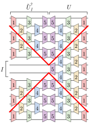
=
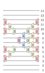
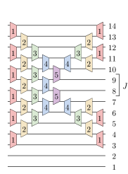
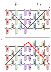
=
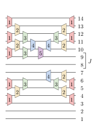
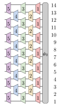
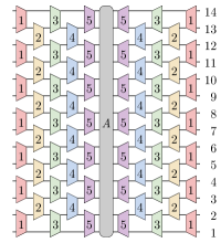
In this section, we study how unitary operators act in the gauge picture. As an instructive example, in Figs. 2 and 3 we depict dynamical variables used in different pictures of quantum dynamics after the time evolution of a quantum circuit. The quantum circuit consists of a composition of unitary operators that each act on pairs of neighboring qubits. Equivalently, the circuit could result from a time-dependent Hamiltonian evolution.
Similar to operators in the local Heisenberg picture (Fig. 2c), the unitaries and (Fig. 3a and 3c) in the gauge picture also grow as time evolves. Figs. 2c and 3 demonstrate the explicit locality of the local variables in the Heisenberg and gauge pictures: over a short time evolution, these local variables are not affected by anything far away. Fig. 3a demonstrates that this locality is achieved via the composition , where cancels out distant unitary evolution.
V.1 Unitary Operators
Let us describe the affect of local unitary operators in the gauge picture using equations. Consider the action of many local unitary operators on the Schrödinger picture wavefunction:
| (43) |
Assume that each unitary acts within patch and that all unitaries commute (e.g. as they do for each layer of unitaries in Fig. 2):
| (44) |
The local gauge picture variables transform as follows:
| (45) | ||||
In analogy to , we define
| (46) |
where denotes a product over all patches that overlap with patch . Note that since [Eq. (32)], which implies that since and commute. Therefore, all of the terms in Eq. (46) commute, and can also be expressed as
| (47) |
To derive Eq. (45), imagine that the local unitaries are applied using a time-independent Hamiltonian with commuting local terms (i.e. ). Then we can use Eqs. (30) and (29) to calculate how and transform:
| (48) | ||||
where denotes a product over all patches that do not overlap with patch . This allows us to calculate the transformation
| (49) |
from [Eq. (32)]. The other transformations in Eq. (45) are extracted from [Eq. (26)] and [Eq. (13)].
VI Measurements
In the Schrödinger picture, a measurement results in a nonlocal collapse of the wavefunction. Most generally, a measurement process can be specified in terms of a collection of Kraus operators , whose squares sum to the identity:
| (50) |
For example, we could take the Kraus operators to be projection operators that project onto the different eigenstates of a Hermitian operator . After the measurement, the wavefunction changes to
| (51) |
with probability
| (52) |
Note that if all measurement outcomes are averaged over, the expectation value of an operator after a measurement is not affected due to Eq. (50).
Let us now consider the result of a local measurement in the gauge picture. We specify the local measurement on a spatial patch using a collection of local Kraus operators that act on the patch . Similar to above, the squared Kraus operators must sum to the identity:
| (53) |
After the measurement, the local wavefunction at patch changes to
| (54) |
with probability
| (55) |
The connections are not affected. In order to maintain consistency with the other spatial patches, all other local wavefunctions must transform as well:
| (56) |
Equation (33) can be used to show that these equations are consistent with the Schrödinger picture. Equation (56) demonstrates that the wavefunction collapse is nonlocal in the gauge picture.
VII Generalized Locality
In this section, we generalize the notion of locality in the gauge picture. The underlying role of a spatial patch is to define a subspace of operators that only act within the spatial patch. Thus, we can generalize the notion of spatial patches to subspaces of operators. That is, instead of letting capital , , and denote spatial patches, we could instead let them denote operator subspaces. The above equations that applied for local operators are generalized to apply to any operator in the subspace . We can therefore generalize the notion of geometric locality to locality between different subspaces of operators, which might e.g. correspond to different energy or charge densities.
We say that two operator subspaces ( and ) do not commute if there exists a pair of operators ( and ), with one from each subspace ( and ), such that the pair does not commute (). The notion of overlapping spatial patches generalizes to non-commuting operator subspaces. Therefore in Eq. (20), the sum generalizes to a sum over all operator subspaces that do not commute with subspace . Similarly, the sum in Eq. (35) generalizes to a sum over all subspaces where any one of these subspaces does not commute with subspace .
Despite the abstractness of this generalization, it does have physical applications. For example, bosonic Hamiltonians (e.g. the Bose-Hubbard model) consisting of bosonic creation and annihilation operators typically exhibit a sense of locality in boson number. That is, for many bosonic Hamiltonians, the action of a Hamiltonian term typically only changes the boson numbers at each site by a small amount. Therefore, we could consider choosing the operator subspaces to consist of the subspace of operators that act at site and only on states with boson number or at site . To be concrete, let denote a boson operator that projects a wavefunction onto the subspace with bosons at site and then changes the boson number at site to . With this notation, the boson number operator at site could be expressed as and the annihilation operator as Then in this example, the subspace consists of the operators spanned by , , , and . In the resulting gauge picture, the operator subspaces and local wavefunctions are indexed by position and local boson number , which results in equations of motion that are explicitly local in both space and local boson number.
We could similarly use the total energy or local energy density to specify the operator subspaces. More generally, we can obtain an extra dimension of locality whenever a model has a conserved (or approximately conserved) charge or energy. For example, consider a collection of spatial patches and a local Hamiltonian where each Hamiltonian term has many (possibly infinitely many) energy levels. Then we could define operator subspaces that consist of the subspace of operators that act within the spatial patch and only on eigenstates of with energy between (with chosen to be sufficiently large that we can capture the necessary operators). In this example, the gauge picture exhibits explicit locality in both space and local energy density.
VIII Conclusion
Having different pictures for understanding the same physics has frequently proved to be invaluable. Furthermore, it is useful when a fundamental property of the physics is explicit in the equations, e.g. as in a Lorentz-invariant Lagrangian. To this end, we studied a picture of quantum dynamics that makes locality explicit in the equations of motions for local wavefunctions. From another point of view, the gauge picture can be thought of as the result of “gauging” the global unitary invariance of Schrödinger’s equation into a local unitary invariance. The gauge picture open several intriguing directions for future research.
VIII.1 New Approximation Technique
Simulating the gauge picture dynamics on a computer can be achieved using a computational time that scales as , where is the number of connections (which typically scales with the system size), is the Hilbert space dimension, is the time complexity for matrix multiplication in practice222For extremely large , an time complexity for matrix multiplication is in principle possible for some Hartnett (2021); Strassen (1969)., is the final time, and is the time step used for numerical integration.333The time complexity is dominated by the time it takes to multiply a connection with another matrix in Eqs. (19) and (20), which must be done times. Although this is more expensive than simulating the Schrödinger picture, in another work Slagle (2023) we show that the gauge picture facilitates a new kind of approximation scheme for improved computational efficiency.
In the Schrödinger picture, truncating the Hilbert space to low-energy states is a common technique to decrease the Hilbert space dimension. For example, tight binding models truncate the Hilbert space to only include the energy bands closest to the chemical potential. However, this truncation technique still requires a Hilbert space dimension that scales exponentially with system size.
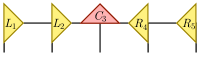
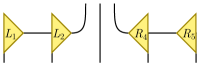
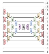
The gauge picture allows a more efficient Hilbert space truncation where a different subspace of states is kept for different patches of space. The utility of a position-dependent Hilbert space truncation is exemplified by matrix product states Orús (2014) (and isometric tensor networks Zaletel and Pollmann (2020)), which are efficient tensor network representations of wavefunctions with area-law entanglement Orús (2014). Figure 4 (adapted from Ref. Slagle (2023)) shows how a matrix product state can be viewed as a wavefunction in a position-dependent truncated Hilbert space. Although position-dependent truncated Hilbert spaces are already used by matrix product states and isometric tensor networks, the gauge picture provides a new way to approximately time evolve wavefunctions using position-dependent truncated Hilbert spaces. Compared to tensor network methods, the gauge picture provides significantly simpler quantum dynamics algorithms for models in two or more spatial dimensions and for models with fermions. See Ref. Slagle (2023) for a more thorough exploration of this approach.
VIII.2 New Deformation of Quantum Mechanics
The gauge picture agrees with the Schrödinger picture when there is no curvature in the gauge connections, i.e. when Eq. (14) is satisfied. Adding curvature to the initial conditions [i.e. adding violations of Eq. (14)] yields a new kind of deformation of quantum theory, which could yield testable experimental predictions for new physics beyond quantum theory. Considering gauge curvature deformations of quantum theory may be appealing since gauge curvature has been a major theme in the Standard Model of particle physics. Furthermore, this deformation explicitly maintains locality, in contrast to Weinberg’s nonlinear deformations of quantum theory Weinberg (1989) which allows supraluminal communications Gisin (1990); Polchinski (1991). However, future research is needed to determine if testable predictions Slagle (2021) can be made that are consistent with previous experiments.
VIII.3 Other Future Directions
Other intriguing future directions include: (1) It is not clear how to describe quantum channels or the Lindblad master equation in the gauge picture. The obstruction is that we used a unitary operator () to cancel out distant unitary dynamics in order to achieve locality; but unitary operators can not cancel out the non-unitary dynamics of quantum channels or the Lindbladian. (2) Does the gauge picture have useful applications for understanding exotic dynamical many-body phenomena, such as out-of-time-ordered correlation functions Swingle (2018); García-Mata et al. (2022), many body localization Nandkishore and Huse (2015); Abanin et al. (2019), or the speed of information propagation Nachtergaele and Sims (2011); Roberts and Swingle (2016); Wang and Hazzard (2020)?
Acknowledgements.
We thank Lesik Motrunich, Sayak Guha Roy, Sagar Vijay, Gunhee Park, and Garnet Chan for helpful conversations. K.S. was supported by the Walter Burke Institute for Theoretical Physics at Caltech; and the U.S. Department of Energy, Office of Science, National Quantum Information Science Research Centers, Quantum Science Center. This research was supported in part by the National Science Foundation Grant No. NSF PHY-1748958 and the Gordon and Betty Moore Foundation Grant No. 2919.02. We also acknowledge funding from the Welch Foundation through Grant No. C-2166-20230405.References
- Deutsch and Hayden (2000) David Deutsch and Patrick Hayden, “Information flow in entangled quantum systems,” Proceedings of the Royal Society of London Series A 456, 1759 (2000), arXiv:quant-ph/9906007 .
- Levin and Wen (2005) Michael A. Levin and Xiao-Gang Wen, “String-net condensation: A physical mechanism for topological phases,” Phys. Rev. B 71, 045110 (2005), arXiv:cond-mat/0404617 .
- Senthil et al. (2004) T. Senthil, Ashvin Vishwanath, Leon Balents, Subir Sachdev, and Matthew P. A. Fisher, “Deconfined Quantum Critical Points,” Science 303, 1490–1494 (2004), arXiv:cond-mat/0311326 .
- Yoshida (2013) Beni Yoshida, “Exotic topological order in fractal spin liquids,” Phys. Rev. B 88, 125122 (2013), arXiv:1302.6248 .
- Hartnett (2021) Kevin Hartnett, “Matrix multiplication inches closer to mythic goal,” Quanta Magazine (2021).
- Strassen (1969) Volker Strassen, “Gaussian elimination is not optimal,” Numerische Mathematik 13, 354–356 (1969).
- Slagle (2023) Kevin Slagle, “Quantum Gauge Networks: A New Kind of Tensor Network,” Quantum 7, 1113 (2023), arXiv:2210.12151 .
- Orús (2014) Román Orús, “A practical introduction to tensor networks: Matrix product states and projected entangled pair states,” Annals of Physics 349, 117–158 (2014), arXiv:1306.2164 .
- Zaletel and Pollmann (2020) Michael P. Zaletel and Frank Pollmann, “Isometric Tensor Network States in Two Dimensions,” Phys. Rev. Lett. 124, 037201 (2020), arXiv:1902.05100 .
- Weinberg (1989) Steven Weinberg, “Testing quantum mechanics,” Annals of Physics 194, 336–386 (1989).
- Gisin (1990) N. Gisin, “Weinberg’s non-linear quantum mechanics and supraluminal communications,” Physics Letters A 143, 1–2 (1990).
- Polchinski (1991) Joseph Polchinski, “Weinberg’s nonlinear quantum mechanics and the einstein-podolsky-rosen paradox,” Phys. Rev. Lett. 66, 397–400 (1991).
- Slagle (2021) Kevin Slagle, “Testing Quantum Mechanics using Noisy Quantum Computers,” (2021), arXiv:2108.02201 .
- Swingle (2018) Brian Swingle, “Unscrambling the physics of out-of-time-order correlators,” Nature Physics 14, 988–990 (2018).
- García-Mata et al. (2022) Ignacio García-Mata, Rodolfo A. Jalabert, and Diego A. Wisniacki, “Out-of-time-order correlators and quantum chaos,” (2022), arXiv:2209.07965 .
- Nandkishore and Huse (2015) Rahul Nandkishore and David A. Huse, “Many-Body Localization and Thermalization in Quantum Statistical Mechanics,” Annual Review of Condensed Matter Physics 6, 15–38 (2015), arXiv:1404.0686 .
- Abanin et al. (2019) Dmitry A. Abanin, Ehud Altman, Immanuel Bloch, and Maksym Serbyn, “Colloquium: Many-body localization, thermalization, and entanglement,” Reviews of Modern Physics 91, 021001 (2019), arXiv:1804.11065 .
- Nachtergaele and Sims (2011) Bruno Nachtergaele and Robert Sims, “Much Ado About Something: Why Lieb-Robinson bounds are useful,” (2011), arXiv:1102.0835 .
- Roberts and Swingle (2016) Daniel A. Roberts and Brian Swingle, “Lieb-robinson bound and the butterfly effect in quantum field theories,” Phys. Rev. Lett. 117, 091602 (2016), arXiv:1603.09298 .
- Wang and Hazzard (2020) Zhiyuan Wang and Kaden R.A. Hazzard, “Tightening the lieb-robinson bound in locally interacting systems,” PRX Quantum 1, 010303 (2020), arXiv:1908.03997 .
