Efficient Diffusion Models for Vision: A Survey
Abstract
Diffusion Models (DMs) have demonstrated state-of-the-art performance in content generation without requiring adversarial training. These models are trained using a two-step process. First, a forward - diffusion - process gradually adds noise to a datum (usually an image). Then, a backward - reverse diffusion - process gradually removes the noise to turn it into a sample of the target distribution being modelled. DMs are inspired by non-equilibrium thermodynamics and have inherent high computational complexity. Due to the frequent function evaluations and gradient calculations in high-dimensional spaces, these models incur considerable computational overhead during both training and inference stages. This can not only preclude the democratization of diffusion-based modelling, but also hinder the adaption of diffusion models in real-life applications. Not to mention, the efficiency of computational models is fast becoming a significant concern due to excessive energy consumption and environmental scares. These factors have led to multiple contributions in the literature that focus on devising computationally efficient DMs. In this review, we present the most recent advances in diffusion models for vision, specifically focusing on the important design aspects that affect the computational efficiency of DMs. In particular, we emphasize the recently proposed design choices that have led to more efficient DMs. Unlike the other recent reviews, which discuss diffusion models from a broad perspective, this survey is aimed at pushing this research direction forward by highlighting the design strategies in the literature that are resulting in practicable models for the broader research community. We also provide a future outlook of diffusion models in vision from their computational efficiency viewpoint.
Index Terms:
Diffusion models, Generative models, Stable diffusion, Text-to-image, Text-to-video, Image synthesis.I Introduction
Deep generative modelling has emerged as one of the most exciting computational tools that is even challenging human creativity [1]. In the last decade, Generative Adversarial Networks (GANs) [91], [92] have received a lot of attention due to their high quality sample generation. However, diffusion models [2, 3, 4] have recently emerged as an even more powerful generative technique, threatening the reign of GANs in the synthetic data generation.
Diffusion models are gaining quick popularity because of their more stable training as compared to GANs, as well as higher quality of the generated samples. These models are able to address some notorious limitations of GANs, like mode collapse, overhead of adversarial learning, and convergence failure [5]. The training process of the diffusion models uses a much different strategy as compared to GANs, which involves contaminating the training data with Gaussian noise and then learning to recover the original data from the noisy one. These models are also found to be suitable from the scalability and parallelizability perspective, which adds to their appeal. Moreover, since their training process is based on applying small modifications to original data and rectifying those, they learn a data distribution whose samples closely follow the original data. Thereby, enabling strong realism in the generated samples. It is thanks to these attributes that the current state-of-the-art in image generation has been strongly influenced by the diffusion models, achieving astonishing results [6, 7, 10].
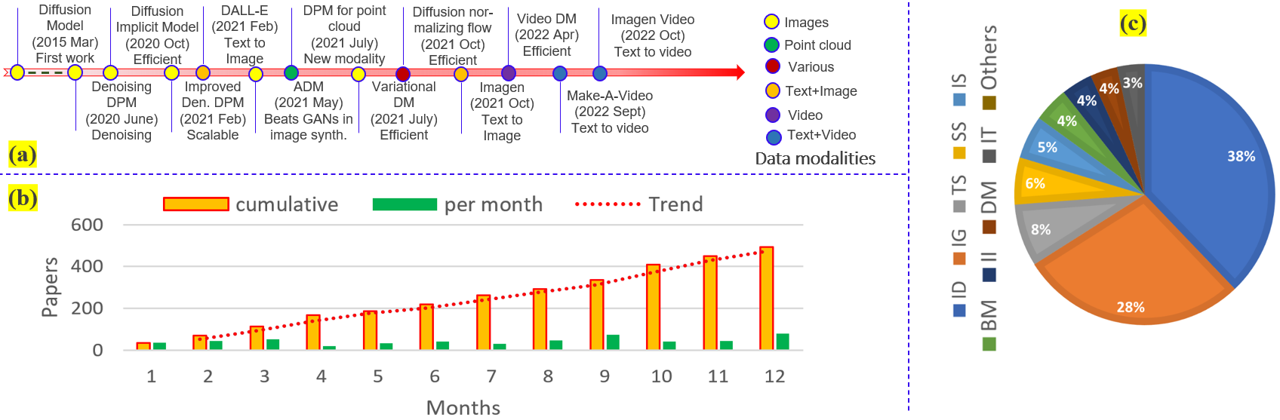
Due to their amazing generative abilities, diffusion models are quickly finding applications in both low- and high-level vision tasks, including but not limited to image denoising [93], [74], inpainting [100], image super-resolution [98], [99], [101], semantic segmentation [94], [95], [96], image-to-image translation [4] etc. Hence, unsurprisingly, since the seminal advancement of diffusion probabilistic models [8] over the original proposal of diffusion modelling [46], there has been a continuous rise in the number of research papers appearing in this direction, and new exciting models are emerging everyday. In particular, diffusion modelling has gained a considerable social media hype after DALL-E [7], Imagen [102], and Stable [80] models that enabled high quality text-to-image generation. This hype has recently been fuelled further by the text-to-video generation techniques, where the videos appear considerably sophisticated [88], [103]. Figure 1 provides statistics and a timeline overview of the recent literature on diffusion models to show their popularity, particularly in the vision community.
Diffusion models belong to a category of probabilistic models that require excessive computational resources to model unobserved data details. Their training process requires evaluating models that follow iterative estimation (and gradient computations). The computational cost becomes particularly huge while dealing with high dimensional data like images and videos [9]. For instance, a high-end diffusion model training in [11] takes 150-1000 V100 GPU days. Moreover, since the inference stage also requires repeated evaluations of the noisy input space, this stage is also computationally demanding. In [11], 5 days of A100 GPU are required to produce 50k samples. Rombach et al. [80] rightly noted that the huge computational requirements to train effective diffusion models present a critical bottleneck in terms of democratizing this technology because the research community generally lacks such resources. It is evident that the most exciting results using diffusion models are first achieved by e.g., Meta AI [88] and Google Research [103] who have an enormous computational power at their disposal. It is also notable that evaluating an already trained model has a considerable time and memory cost because the model may need to run for multiple steps (e.g., 25-1000) to generate a sample [10]. This is a potential hindrance in the practical applications of diffusion models, especially in resource constrained environments.
In the contemporary era of large-scale data, early works on diffusion models focused on high-quality sample generation, largely disregarding the computational cost [8, 11, 12]. However, after achieving reasonable quality milestones, the more recent works have also started to consider computational efficiency, e.g., [80], [97], [60]. In particular, to address the genuine drawback of a slow generation process at the inference stage, a new trend is setting up for the more recent works, focusing on efficiency gains. In this review article, we collectively term the diffusion models evolved under the computational efficiency perspective, efficient diffusion models. These are the emerging models that are more valuable to the research community because they demand accessible computational resources. Whereas progress is being consistently made in terms of improving the computational efficiency, diffusion models are still far slower than GANs in terms of sample generation [13, 14]. We review the existing works concerned with efficiency without sacrificing the high quality of sample generation. Moreover, we discuss the trade-offs between the model speed and sampling quality.
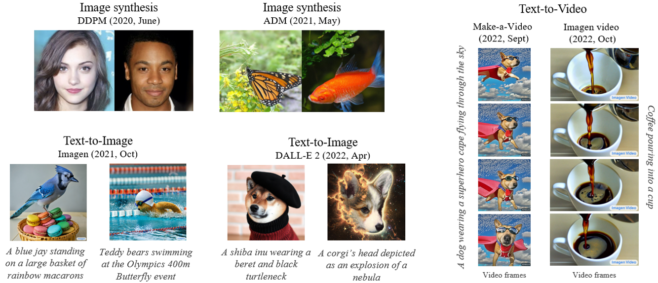
Why model efficiency is critical? Diffusion models have been able to produce an astonishing quality of images and videos, virtually requiring no effort on their users’ part - see Fig. 2. This foretells a widespread usage of these models in the daily-life application domains, such as entertainment industry. The creative abilities of diffusion models, or any AI platform, does not come for free. High-quality generative modeling is energy-intensive, and the higher the quality demand, the more power it consumes. Training a sophisticated AI model needs time, money, and power [15, 16], leaving behind a significant carbon footprint. To put things into a perspective, OpenAI trained GPT-3 model [17] On 45 terabytes of data. Nvidia trained the final version of MegatronLM, a language model comparable to but smaller than GPT-3, using 512 V100 GPUs for nine days. A single V100 GPU may consume up to 300 watts. If we estimate the power consumption of 250 watts, 512 V100 GPUs utilise 128,000 watts or 128 kilowatts (kW) [18]. Running for nine days requires 27,648 kilowatt hours of power for the MegatronLM. The average home consumes 10,649 kWh per year as per the US Energy Information Administration. Implying, training MegatronLM required nearly as much energy as three houses use in a year. Among the currently most hyped diffusion models (due to their ability to perform text-to-image task), e.g., DALL-E [7], Imagen [102], and Stable [80], Stable is by far the most efficient because its diffusion process is mainly carried out in a lower dimension latent space. However, even this model’s training requires an energy equivalent to burning nearly 7,000 kgs of coal111Computed with https://mlco2.github.io/impact/#compute. Not to mention the text-to-image diffusion models already rely on language models such as GPT-3 mentioned above. Other diffusion models, especially for the more complex tasks, e.g. text-to-video, are expected to require orders of magnitude more energy222The carbon footprint calculations are not possible from the details provided in the original papers.. Hence, due to the fast growing popularity of these models, it is critical to focus on more efficient schemes.
Motivation and uniqueness of this survey: Since the diffusion models have recently received a significant attention of the research community, the literature is experiencing a large influx of contributions in this direction. This has also led to review articles surfacing recently. Among them, Yang et al. [3] reviewed the broad direction of diffusion modelling from the methods and applications viewpoint, and Cao et al. [2] also discussed diffusion models more broadly. More related to our review is [4], which focuses on the diffusion model in the vision domain. On one hand, all these reviews already surfaced before this direction fully matured. For instance, the breakthrough of high quality text-to-video generation with diffusion models [88], [103] is actually achieved after the appearance of all these surveys. On the other hand, none of these surveys focuses on computational efficiency of the models, which is the central aspect in pushing this research direction forward. Hence, these surveys leave a clear open gap. We aim at addressing that by highlighting the underlying schemes of the techniques that are improving the computational efficiency of diffusion models. Our comprehensive review of the existing methods from this pragmatic perspective is expected to advance this research direction in the ways not covered by the reviews appeared during the preparation of this article333We note that this manuscript is still a work in progress, which will be updated in the future by improving its quality and including further progress in this direction..
The rest of the article is organised as follows: Section II provides an overview of diffusion models with a brief discussion on three representative architectures. Section III provides a description of design choices and discusses how these choices lead to computation-efficient designs. In Section V compares representative works w.r.t quality and efficiency trade-off. Section VI discusses future work directions, followed by a conclusion.
II An Overview of Diffusion Models
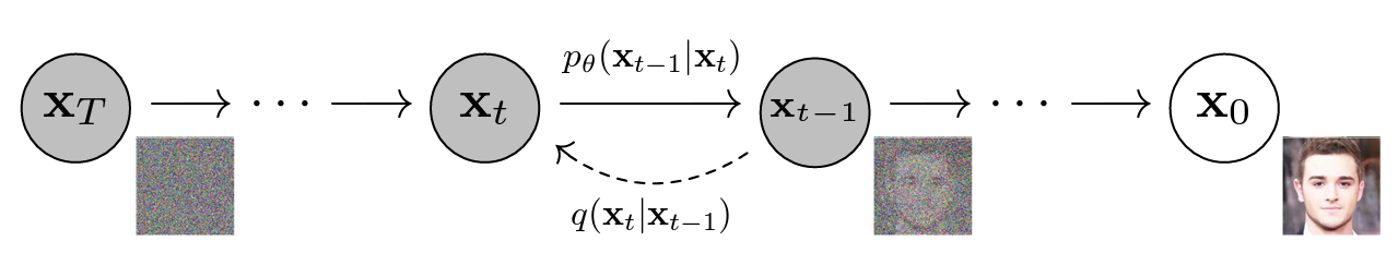
The original idea of the probabilistic diffusion model is to model a specific distribution from random noise. Therefore, the distributions of the generated samples should be as close as those of the original samples. It includes a forward process (or diffusion process), in which complex data (generally an image) is progressively noised, and a reverse process (or reverse diffusion process), in which noise is transformed back into a sample from the target distribution. Here, we describe three models in particular due to their influence on efficient diffusion architecture. It includes denoising diffusion probabilistic models (DDPM) [8], latent diffusion models (LDM) [10] and Feature Pyramid Latent Diffusion Model [19].
II-A The Baseline: Denoising diffusion probabilistic models (DDPM):
Suppose we have an original data point sampled from a real data distribution . Let’s define a forward diffusion process where we gradually add a small amount of Gaussian noise to the samples, resulting in a series of noisy samples . The step sizes are controlled by a variance schedule .
| (1) |
The actual strength of diffusion models, however, is the reverse process called reverse diffusion, as the goal of training a diffusion model is to learn the reverse process. It can be done by training a neural network o approximate these conditional probabilities in order to run the reverse diffusion process.
| (2) |
The reverse conditional probability is tractable when conditioned on
| (3) |
The reverse Markov transitions that maximise the probability of the training data are used to train a diffusion model. Training in practice is similar to reducing the variational upper bound on the negative log probability. Because this configuration is extremely similar to VAE, we may apply the variational lower limit to optimise the negative log-likelihood.
| (4) |
To make each component in the equation analytically computable, the objective may be reformulated as a mixture of many KL-divergence and entropy terms. Let us label each component of the variational lower bound loss separately:
| (5) | ||||
Because every KL term in (excluding ) compares two Gaussian distributions, they can be calculated in closed form. In the reverse diffusion process, a neural network is trained to approximate the conditioned probability distributions. As is available as input at training time, the Gaussian noise term could be reparameterized as:
| (6) |
Empirically, the training the diffusion model works better with a simplified objective that ignores the weighting term:
| (7) |
The final simple objective is , where C is a constant not depending on .
Model Efficiency: It is very slow to generate a sample from DDPM by following the Markov chain of the reverse diffusion process, as can be up to one or a few thousand steps. For example, takes around 20 hours to sample 50k images of size 32 × 32 from a DDPM but less than a minute to do so from a GAN on an Nvidia 2080 Ti GPU.
II-B Latent diffusion model (LDM):
These models perform the diffusion process in latent space rather than pixel space, lowering training costs and increasing inference speed. It is driven by the discovery that the majority of picture bits contribute to perceptual details and that the semantic and conceptual composition persists after extreme compression. With generative modelling learning, LDM loosely decomposes perceptual compression and semantic compression by first cutting out pixel-level redundancy with autoencoder and then manipulating/generating semantic ideas with diffusion process on learnt latent.
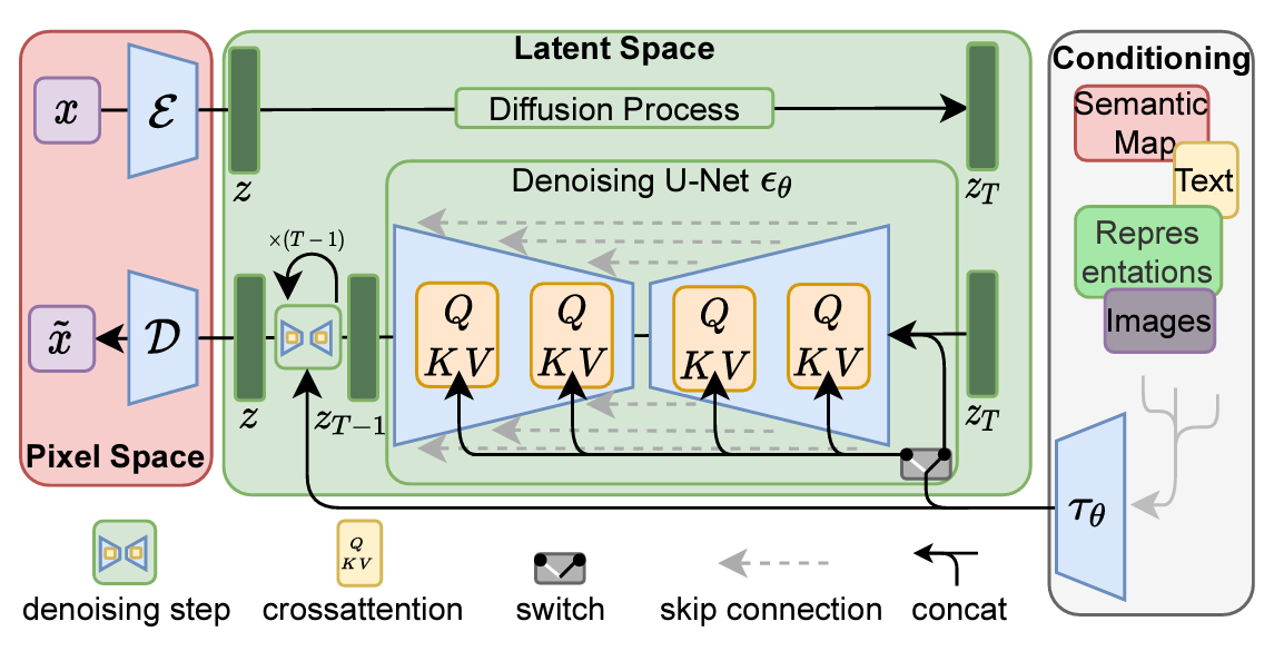
An autoencoder model is used in the perceptual compression process. A encoder is used to compress the input picture to a smaller 2D latent vector. , where the downsampling rate . Then an decoder reconstructs the images from the latent vector, To prevent arbitrarily large variance in the latent spaces, the research investigated two kinds of regularisation in autoencoder training.
The neural backbone of the LDM model is realized as a time-conditional UNet. The model has the ability to build the underlying UNet primarily from 2D convolutional layers and further focus the objective on the perceptually most relevant bits using the reweighted bound, which now reads:
| (8) |
On the latent vector , the diffusion and denoising processes take place. The denoising model is a time-conditioned U-Net that has been supplemented with a cross-attention mechanism to manage flexible conditioning information for picture production (e.g. class labels, semantic maps, blurred variants of an image). The design is akin to fusing representations of various modalities into a model with a cross-attention mechanism. Each kind of conditioning information is associated with a domain-specific encoder , which projects the conditioning input to an intermediate representation that can be translated into the cross-attention component, :
| (9) |
where,
| (10) |
and
| (11) |
(Source: )
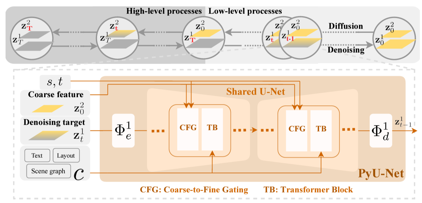
II-C Feature Pyramid Latent Diffusion Model ( Frido):
Frido decomposes the input image into scale-independent quantized features and then obtains the output result through coarse-to-fine gating. In short, the author first uses multi-scale MS-VQGAN (Multi-Scale VQGAN), encodes the input image into the latent space, and then uses Frido to do diffusion in the latent space. The encoder of MS-VQGAN encodes the input image into N-scale latent variables, similar to an image pyramid, but in latent space. The low-level latent variables keep lower-level visual details, while the high-level latent variables keep high-level shapes and structures. Then the decoder decodes the obtained hidden variables of all scales into the output image. The size of the pyramid of this hidden variable also decreases with the number of layers, and each layer is half of the upper layer. In this way, both high-level semantic information and more low-level details can be maintained. Given an image , the encoder E first produces a latent feature map set of N scales
| (12) |
Next is the diffusion model in the latent space. The previous methods directly implement the diffusion model on all hidden variables, but the method in this paper includes multiple scales. So the author sequentially performs diffusion on different scales, and each scale T step requires . Then the diffusion operation of adding noise forward first destroys the details of the image, then the high-level shape, and finally, the structure of the entire image.
The corresponding process of Denoising is a process from high level to low level. Based on the previous U-Net, the author proposes a feature pyramid U-Net (PyU-Net) [19] to realize the denoising process at multiple scales. Two innovations of this PyU-Net: By adding a lightweight network to each scale, the hidden variables of each layer are mapped to the same dimension so that they can be unified as the input of U-Net. Correspondingly, it is also necessary to add light weight to the input of U-Net. The amount of network to remap back to the dimension of the current scale information. Coarse-to-fine gating has been added to allow low-level denoises to utilize existing high-level information. To train more effectively, the author uses a teacher forcing trick, Works with teacher forcing to maintain training efficiency while preventing overfitting, and enables UNet to obtain information on the current scale level and time step. Finally, another level-specific projection decodes the U-Net output to predict the noise added on z with the following objective.
| (13) |
III Effective Strategies for Efficient Diffusion Models:
The diffusion model needs Reconstructing data distribution that needs sampling. The major hurdle in the way of efficient diffusion models is their sampling process inefficiency, as it is very slow to generate samples from DDPM. Diffusion models rely on a long Markov chain of diffusion steps to generate samples, so it can be quite expensive in terms of time and computing.
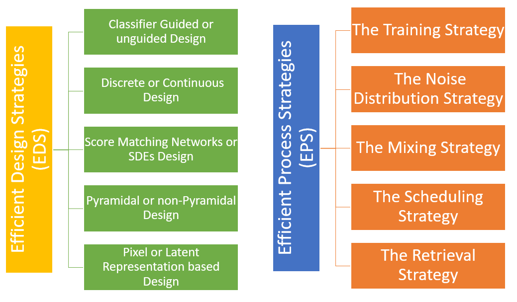
Significant efforts have been made to accelerate the sampling procedures in recent years. We divide these influencing strategies into two categories: Efficient Design Strategies (EDS), which recommend modifications to the design of baseline diffusion models and Efficient Process Strategies (EPS), which suggest ways to improve the efficiency of diffusion models or speed up the sampling process. However, these strategies are inferred by revising the literature, and future work may include some novel strategies not mentioned below.
(Source: )
III-A Efficient Design Strategies (EDS)
These strategies are based on the architecture of diffusion models. Table 1 includes some representative work in each architectural category that is included. A brief description of each category and its influence on the efficiency of diffusion models are discussed below:
| Architecture | Model | Citation | Strategy |
|---|---|---|---|
| Guided | ADM | [11] | Classifier guidance and upsampling |
| Not-Guided | CFDG | [20] | Classifier-free guidance |
| Guided | SDEDIT | [21] | Stochastic Differential Editing |
| Guided | VDM | [22] | Reconstruction-guided sampling |
| Guided | SDG | [23] | Semantic Diffusion Guidance |
| Not-Guided | Make-A-Scene | [24] | Classifier-free guidance |
| Not-Guided | VQ-Diffusion | [25] | DiscreteClassifier-free Guidance |
| Discrete | DDPM | [8] | Discrete data |
| Continuous | DP stride | [26] | Continuous Time Affine Diffusion Processes |
| Continuous | FastDPM | [27] | Continuous diffusion steps |
| Continuous | DSB | [28] | Diffusion Schrödinger Bridge |
| Discrete | VQ-Diffusion | [25] | Discrete Classifier-free Guidance |
| Score Network | BDDM | [29] | score and scedulng network |
| Score Network | CLD | [30] | Score matching objective |
| Score Network | GGDM | [33] | Sample quality scores. |
| SDE | DSB | [28] | Diffusion Schrödinger Bridge |
| Score Network | ScoreFlow | [34] | Inproving likelihood of Scores |
| SDE | EMSDE | [35] | Adaptive step sizes |
| Pyramidal | CDM | [36] | Cascading pipelines |
| Pyramidal | Frido | [19] | Pyramid diffusion |
| Pyramidal | PDDPM | [37] | Pyramidal reverse sampling |
| Non-Pyramidal | Blur diffusion | [38] | Frequency Diffusion at variable speeds |
| Non-Pyramidal | NWDM | [39] | Frequency domain diffusion |
| Latent | ILVR | [40] | Iterative Latent Variable Refinement |
| Latent | LDM | [10] | latent space |
| Latent | latent DDIM | [41] | Semantic latent interpolation |
| Latent | INDM | [42] | Linear diffusion on the latent space |
| Pixel | DDPM | [8] | image upsampling and downsampling |
| Pixel | DDIM | [43] | image upsampling and downsampling |
1- Classifier Guided or unguided Design: Classifier guidance is a recently developed strategy for balancing mode coverage and sample fidelity in post-training conditional diffusion models, in the same way, that low-temperature sampling or truncation is used in other forms of generative models. An example is a work by Nichol [44] that trained a classifier on noisy image To explicit incorporate class information into the diffusion process, and use gradients to guide the diffusion sampling process toward the conditioning information (e.g. a target class label) by altering the noise prediction.
Guidance is a trade-off: it enhances adherence to the conditioning signal and overall sample quality, but at a high cost to vary. While classifier guidance successfully trades off quality metrics (IS and FID) as expected from truncation or low-temperature sampling, it is nonetheless reliant on gradients from an image classifier.
Classifier-free guidance [20] achieves the same effect without such gradients. Classifier-free guidance is an alternative method of modifying gradients to have the same effect as classifier guidance but without a classifier. It increases sample quality while decreasing sample diversity in diffusion models.
2- Discrete or Continuous Design: The Diffusion Process is a continuous example that may be characterized by a Stochastic Differential Equation.Probability Flow ODE (Diffusion ODE) is the continuous-time differential equation [45]. Denoising diffusion probabilistic models (DDPMs) [8] have shown impressive results in image and waveform generation in continuous state spaces.
Denoising diffusion models have produced both remarkable log-likelihood scores on numerous common picture datasets and high-quality image production in continuous situations. Many datasets are discrete, but for the convenience of modeling, they are frequently embedded in a continuous space and modeled continuously.
Structured corruption processes appropriate for text data, using similarity between tokens to enable gradual corruption and denoising. Diffusion models with discrete state spaces were first introduced by Sohl-Dickstein et al.[46] who considered a diffusion process over binary random variables. Considered a simple 2×2 transition matrix for binary random variables. Hoogeboom et al. [47] later extended this to categorical variables, proposing a transition matrix.
This, however, can lead to tough modeling concerns such as ”de-quantization” blockages, weird gradient issues, and difficulties understanding log-likelihood metrics. All of these concerns are avoided by representing discrete data separately. Instead of transitioning uniformly to any other state, for ordinal data, discrete models imitate a continuous space diffusion model by using a discretized, truncated Gaussian distribution.
In terms of efficient design, discrete diffusion design is preferable as it helps reduce the number of samples. Diffusion models with discrete state spaces were first introduced by Sohl-Dickstein et al. [46], who considered a diffusion process over binary random variables.
Even though diffusion models have been presented in both discrete and continuous state spaces, much current work has concentrated on Gaussian diffusion processes that operate in continuous state spaces (e.g. for real-valued image and waveform data).
3- Score Matching Networks or SDEs Design: The score network may be used to create an ODE (”scoring-based diffusion ODE”) for evaluating precise probability [30, 48]. They simulate the distribution of data by matching a parameterized score network with first-order data score functions. The gradient of the log-likelihood concerning the random variable x is defined as the score.
| (14) |
The purpose of score-matching is to reduce the difference between and by optimizing the Fisher divergence. It has been used in medical applications such as low-dose computed tomography (LDCT), resulting in a low signal-to-noise ratio (SNR) and potential impairment of diagnostic performance. The Diffusion Probability Model for Conditional Noise Reduction (DDPM) has been shown to improve LDCT noise reduction performance with encouraging results at high computational efficiency. Especially considering the high sampling cost of the original DDPM model, the fast ordinary differential equation (ODE) solver can be scaled for greatly improved sampling efficiency. Experiments [49] show that accelerated DDPM can achieve 20X speedup without degrading image quality.
| Process | Model | Citation | Strategy |
|---|---|---|---|
| Training | FSDM | [50] | Conditioned on a small class set |
| Training | VDM | [22] | Joint training from image and video |
| Training | MMDM | [51] | Argmax Flows and Multinomial Diffusion |
| Training | P2 | [52] | Perception PrioritizedWeighting |
| Training | DDRM | [53] | Pre-trained demonising diffusion |
| Noise Ditribution | DGM | [54] | noise from Gamma distribution |
| Noise Ditribution | GGDM | [33] | Differentiable Diffusion Sampler Search |
| Noise Ditribution | NEDM | [55] | Noise Schedule Adjustments |
| Noise Ditribution | CCDF | [56] | Non Gaussian initialisation |
| Noise Ditribution | Cold Diffusion | [57] | Deterministic noise degradation |
| Noise Ditribution | BDDM | [29] | Non-isotropic noise |
| Noise Ditribution | GDDIM | [58] | Mixture Gaussian, Gamma Distribution |
| Mixing | DiVAE | [59] | Input image embedding |
| Mixing | FastDPM | [27] | Unified framework |
| Mixing | DiffFlow | [60] | Normalizing flow and diffusion |
| Mixing | MMDM | [51] | Argmax Flows Multinomial Diffusion |
| Mixing | LDM+DDIM | [61] | Latent Implicit Diffusion |
| Mixing | Diffusion-GAN | [62] | Gaussian mixture distribution |
| Scheduling | DP stride | [26] | Learning time schedule by optimization |
| Scheduling | Bit Diffusion | [63] | Asymmetric Time Intervals |
| Scheduling | DiffusionTimes | [64] | Trade off on diffusion time |
| Scheduling | ProgressiveDistillation | [65] | Deterministic diffusion sampler |
| Scheduling | ES-DDPM | [66] | Early Diffusion Stoppage |
| Scheduling | CMDE | [67] | Multiscale diffusion |
| Scheduling | FHDM | [68] | Termination at a random first hitting time |
| Scheduling | IDSD | [69] | Stochastic sampling |
| Retreival | KNN-Diffusion | [70] | KNN adapted training |
| Retreival | RDM | [71] | Database subset conditioning |
| Retreival | RDM | [72] | Informative samples Conditioning |
A stochastic differential equation (SDE) [21] is a differential equation where one or more of the terms is a stochastic process, resulting in a solution, which is itself a stochastic process.
Diffusion ODE can be seen as a semi-linear form by which the discretization errors are reduced. DPM-solver accomplished the SOTA within 50 steps on CIFAR-10 [73], and it can generate high-quality images) with ten steps, which is an extensive upgrade.
Compared to traditional diffusion methods with discrete steps, numerical formulations of differential equations achieve more efficient sampling with advanced solvers. Inspired by Score SDE and Probability Flow (Diffusion), ODE.
4- Pyramidal or non-Pyramidal Design: Pyramidal approaches to training the diffusion model such that it can understand the different scales of the input by giving coordinate information as a condition. These models concatenate an input image and coordinate the values of each pixel. Then, random resizing to the target resolution is applied to the merged input. The resized coordinate values are encoded with the sinusoidal wave, expanded to high dimensional space, and act as conditions when training. Benefiting from the UNet-like model structure [59], the cost function is kelp invariant to all different resolutions so that the optimization can be performed with only a single network. The multi-scale score function, the sampling speed, which is the most critical disadvantage of the diffusion models, can also be made much faster compared to a single full DDPM by a reverse sampling process.
Therefore, the pyramidal or multiscale approach provides better efficiency to diffusion models.
5- Pixel or Latent Representation-based Design: The majority of a digital image’s bits correspond to insignificant information. While DMs allow for the suppression of semantically meaningless information by minimizing the responsible loss term, gradients (during training) and the neural network backbone (during training and inference) must still be evaluated on all pixels, resulting in redundant computations and unnecessarily expensive optimization and inference.
The model class Latent Diffusion Models (LDMs) provide efficient image generation from the latent space with a single network pass. LDMs work in the learned latent space, which exhibits better-scaling properties concerning the spatial dimensionality.
Therefore, latent models are efficient compared to pixel-based designs.
III-B Efficient Process Strategies (EPS)
These strategies target the improvement of the diffusion process itself. Table 2 includes some representative work in each process category that is included. A brief description of each category and its influence on the efficiency of diffusion models are discussed below:
1- Training Strategy: To enhance sampling speed, several strategies focus on modifying the pattern of training and noise schedule. However, re-training models require more processing and increase the risk of unstable training. Fortunately, there is a family of approaches known as training-free sampling that directly augments the sample algorithm using a pre-trained model. The purpose of advanced training-free sampling is to offer an efficient sampling method for learning from a pre-trained model in fewer steps and with improved accuracy. Analytical approaches, implicit sampler, differential equation solver sampler, and dynamic programming adjustment are the three types.
By using a memory technique, dynamic programming may traverse all options to discover the optimal solution in a relatively short amount of time. In comparison to previous efficient sampling approaches, dynamic programming methods discover the optimal sample path rather than constructing strong steps that decrease error more rapidly.
2- Noise Distribution Strategy: Unlike DDPM [8], which defines noise scale as a constant, research into the effect of noise scale learning has received a lot of interest [55], because noise schedule learning also counts during diffusion and sampling. Each sample step may be seen as a random walk on the direct line heading to the preceding distribution, demonstrating that noise reduction may help the sampling operation. The random walk of random noise is guided by noise learning in both the diffusion and sampling processes, resulting in more efficient reconstruction.
The underlying noise distribution of the diffusion process is Gaussian noise in most known approaches. Fitting distributions with more degrees of freedom, on the other hand, may increase the performance of such generative models. Other noise distribution forms for the diffusion process are being researched. The Denoising Diffusion Gamma Model (DDGM) [54] demonstrates that noise from the Gamma distribution improves picture and voice creation.
The sample obtained from random noise will be tweaked anew in each sampling step to get closer to the original distribution. However, sampling with diffusion models requires too many steps, resulting in a time-consuming condition [74].
3- The Mixing or Unifying Strategy: Mixed-Modeling entails incorporating another form of the generative model into the diffusion model pipeline to make use of others’ high sampling speed, such as adversarial training networks and autoregressive encoders, as well as high expressiveness, such as normalizing flow [75, 60, 62]. Thus, extracting all of the strengths by combining two or more models with a specified pattern results in a possible upgrade known as Mixed-modeling.
The goal of diffusion scheme learning is to investigate the influence of different diffusion patterns on model speed. Truncating both the diffusion and sampling processes, resulting in shorter sampling time, is advantageous for lowering sampling time while enhancing producing quality. The main goal behind truncating patterns is to generate less dispersed data using various generative models such as GAN [76] and VAE [77].
By gradually distilling knowledge from one sample model to another, a diffusion model may be enhanced [78]. Before being taught to create one-step samples as near to teacher models as possible, student models re-weight from teacher models in each distillation step. As a consequence, student models can cut the number of sample steps in half during each distillation operation.
The acceleration approach for generalized diffusion aids in the solution of a wide range of models and provides insights into effective sampling mechanisms. Other related research establishes the relationship between the diffusion model and denoising score matching, which may be considered one sort of unification.
4- Scheduling Strategy: Improving the training schedule entails updating classic training methods such as the diffusion scheme, noise scheme, and data distribution scheme, all of which are independent of sampling.
When solving the diffusion SDE, decreasing the discretization step size helps speed up the sampling operation. Such techniques, however, would result in discretization mistakes and significantly impact model performance [60]. As a result, several strategies for optimizing the discretization scheme with a time to minimize sampling steps while maintaining excellent sample quality have been devised.
To create a prediction, the Markov process only uses the sample from the previous phase, which restricts the use of plentiful earlier data. In contrast, the transition kernel of the Non-Markovian process may rely on more samples and use more information from these samples. As a result, it can create accurate predictions with a high step size, which speeds up the sampling method.
Alternatively, by just performing certain phases of the reverse process to obtain samples, one might trade sample quality for sampling speed. Some sampling can be accomplished by pausing or truncating the forward and reverse processes early on or by retraining student networks and bypassing partial phases through knowledge distillation.
Diffusion sampling may be accomplished in a few steps with the use of strong conditioned conditions. Early Stop (ES) DDPM produced implicit distribution by producing previous data with VAE, which learned the latent space [66].
As previously stated, it generally takes the same number of steps for the generative process as it does for the diffusion process to reconstruct the original data distribution in DDPM [8]. However, the diffusion model has the so-called decoupling property in that it does not require the same number of steps for diffusing and sampling. The implicit sampling approach, which is based on the generative implicit model, includes deterministic diffusion and jump-step sampling. Surprisingly, implicit models do not require re-training since the forward’s diffusion probability density is constant at all times. DDIM[43] uses continuous process formulation to tackle the jump-step acceleration problem.
5- Retrieval Strategy: During training, RDMs [71, 72] obtain a collection of closest neighbors from an external database, and the diffusion model is conditioned on these informative samples. Retrieval-augmentation works by looking for photos that are similar to the prompt you offer and then letting the model view them during creation.
During training, the diffusion model is fed comparable visual characteristics obtained via CLIP and from the vicinity of each training instance. By using CLIP’s combined image-text embedding space [79], the model delivers very competitive performance on tasks for which it has not been explicitly trained, such as class-conditional or text-image synthesis, and may be conditioned on both text and picture embeddings improving its performance. Retrieval-Augmented Diffusion Models [80] are recently used for the text-guided synthesis of artistic images efficiently.
Retrieval-Augmented Text-to-Image Generator (Re-Imagen), [81] is a generative model that uses the extracted information to produce highly faithful images even for rare or invisible entities. At a text message, Re-Imagen accesses an external multimodal knowledge base to retrieve the relevant pairs (image, text) and uses them as references to generate the image.
IV Comparative Performance and Discussion
In this section, we will discuss the comparative performance of different diffusion models, particularly in terms of sampling efficiency and the number of parameters. We will also discuss future work directions to lead new research into this exciting area.
As mentioned earlier, the research focus to date was heavily on increasing the quality of generated samples, and stable diffusion has changed the course with a focus on efficiency. Before comparative analysis, we will mention the important quality and efficiency metrics being used in the research community to compare diffusion models’ performance.
Inception Score (IS): The inception score is designed to value both the variety and resolution of created pictures based on the ImageNet dataset [82]. It is split into two sections: diversity measurement and quality measurement. Diversity is measured in terms of the class entropy of generated samples: the higher the entropy, the more diverse the samples. Quality is measured using entropy and the similarity between a sample and the relevant class pictures because the samples will have a higher resolution if they are closer to the ImageNet dataset’s specific class of pictures.
2 Frechet Inception Distance (FID): Although the Inception Score includes suitable assessment approaches, the establishment is dependent on a particular dataset with 1000 classes as well as a trained network that includes randomnesses such as initial weights and code structure. As a result, the bias between ImageNet and real-world photos may result in an incorrect result. Furthermore, the sample batch size is substantially lower than 1000 classes, resulting in low-belief statistics. To address the bias from specific reference datasets, FID is proposed [83]. Using the mean and covariance, the score calculates the distance between the real-world data distribution and the produced samples.
3 Negative Log Probability (NLL) Negative log-likelihood is viewed as a common assessment metric that describes all patterns of data distribution by Razavi et al. There has been a lot of effort on normalising flow fields [and VAE fields employ NLL as one of the assessment options. Some diffusion models, such as enhanced DDPM, consider the NLL to be the training aim.
Some efficiency metrics include the following:
1- Sampling speed or throughput: Fast sampling is one major efficiency target of diffusion models alongside sampling quality metrics. Sample/second. A simple measure will be the number of steps in generating these samples, as a low number of steps is preferable.
2- Computing Workload: Modern HPC data centers are key to solving heavy computing workloads like diffusion models. As NVIDIA Tesla V100 Tensor Core is one of the most advanced data center GPUs, some works have compared the performance of the diffusion model by V100 days.
3- Model Complexity: Number of Parameters: Model parameters are important metrics. However, it is hard to directly relate it to efficiency as more parameters in new heavy and best-performing models are intensive in the number of parameters. However, if the same performance can be achieved with a low number of parameters, that indicates model efficiency.
However, compared to well-established quality metrics, efficiency metrics are still not standardized, and open challenges and benchmarks based on efficiency metrics are still missing. This is another direction to contribute to diffusion model efficiency research.
Image Inpainting has recently become an important research problem due to the rise of generative image synthesis models [44, 40, 84, 85]. Most inpainting solutions perform well on object removal or texture synthesis, while semantic generation is still difficult to achieve. To address these issues, NTIRE 2022 [84] Image Inpainting Challenge was introduced with the target to develop solutions that can achieve a robust performance across different and challenging masks while generating compelling semantic images. The proposed challenge consists of two tracks: unsupervised image inpainting and semantically-guided image inpainting. For Track 1, the participants were provided with four datasets: FFHQ, Places, ImageNet, and WikiArt, and trained their models to perform a mask-agnostic image inpainting solution. For Track 2, FFHQ and Places.
Overall, diffusion models showed excellent results in image painting, as they can be applied to this task without direct supervision. In this challenge, these methods were tested on 7,000 images per dataset. However, the winner of the challenge relies on a Latent Diffusion Model (LDM) cite LDM system, which performed the noise reduction process at a latent representation rather than at the pixel level, drastically reducing the inference time to an average of 10 seconds per image size of 512 × 512.
| Model | Year | FID | Steps | Parameters M |
|---|---|---|---|---|
| PGGAN | 2017 | 8.03 | NA | 23.1 |
| DDGAN | 2021 | 7.64 | NA | - |
| StyleSwin | 2021 | 3.25 | NA | - |
| ADM | 2021 | 1.9 | 1000 | - |
| LDM | 2022 | 2.95 | 200 | 1.9 |
| Model | FLOP | Parameters | Inference Time |
|---|---|---|---|
| LDM-8 | 37.1 G | 589.8 M | 0.82547 |
| Frido | 37.3 G | 1.179 B | 1.02865 |
| Dido-gating | 39.7 G | 697.8 M | 0.91782 |
To find the impact of latent diffusion model [10] on emerging trends in literature, we use bibliographic networks. For this purpose, we use a clustering approach. In cluster analysis, the number of sub-problems is set by the resolution. The greater the value of this parameter, the more clusters will be created. We tried to minimize the number of clusters to focus on the most representative work in terms of relevance ad impact, which resulted in only three clusters based on 50 research papers. Fig. 7 displays these clusters in three primary colors, and Table lists one representative papers in each cluster. Such visualization of a bibliometric network provides an automated insight into relevant literature that can not be figured out manually. This visualization and its depth of understanding helped us to revise our taxonomies, which are discussed in the following sections.
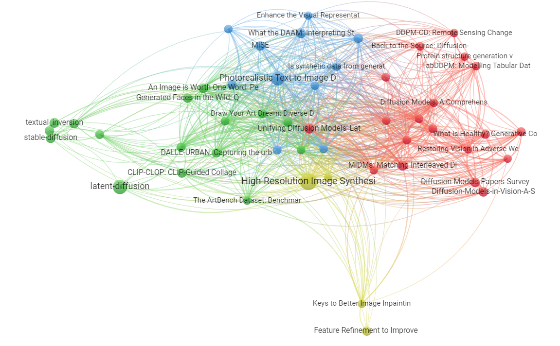
| Cluster | Research Paper: The Title |
|---|---|
| Yellow | High-Resolution Image Synthesis with Latent Diffusion Models |
| Green | Text-Guided Synthesis of Artistic Images with Retrieval-Augmented Diffusion Models |
| Blue | What the DAAM: Interpreting Stable Diffusion Using Cross Attention |
| Red | Unifying Diffusion Models’ Latent Space, with Applications to CycleDiffusion and Guidance |
V Future Work Directions
The popularity, usability, and creativity of diffusion models are attracting new research efforts in the computer vision community, especially after the efficient use of computing resources and open source availability of stable diffusion. It is fair to say that stable diffusion has proved to be a game-changing model. However, new work in literature is emerging every day that addresses other challenges. Some of the emerging research directions are as follows:
-
•
Retrieval-augmentation works by looking for images similar to the specified prompt and then the model can see them during generation.
-
•
Another emerging area is the development of Few-Shot Diffusion Models (FSDM), which present a framework for few-shot generation leveraging conditional DDPMs. These models are trained to adapt the generative process conditioned on a small set of images from a given class by aggregating image patch information using a set-based Vision Transformer (Vit). A new approach like DreamBooth [86] is the ”personalization” of text-to-image diffusion models (specializing them to users’ needs). Given as input just a few images of a subject, such models can fine-tune a pre-trained text-to-image model such that it learns to bind a unique identifier with that specific subject. By leveraging the semantic prior embedded in the model with a new autogenous class-specific prior preservation loss, these models enable synthesizing the subject in diverse scenes, poses, views, and lighting conditions that do not appear in the reference images. CycleDiffusion is introduced by [32] that shows that large-scale text-to-image diffusion models can be used as zero-shot image-to-image editors. It can guide pre-trained diffusion models and GANs by controlling the latent codes in a unified, plug-and-play formulation based on energy-based models.
-
•
In the past, most text-to-image models were developed as propriety applications. However, the coming of stable diffusion open source has initiated another trend that will help evolve diffusion research.
-
•
Another new research direction is innovative architectures for video diffusion models [87, 3] which is a natural extension of the standard image architecture. This architecture may use joint training from image and video data to generate long and higher-resolution videos. Generation of video without text-video data can introduce efficient designs like demonstrated [88].
-
•
Diffusion models are promising candidates for human movement due to their many-to-many nature, but they tend to be resource-intensive and difficult to control. Motion Diffusion Model (MDM) , a carefully tuned classifier-free generative diffusion-based model is introduced for the human motion domain. The model is based on a transformer and combines knowledge from the motion generation literature. It uses sample prediction rather than noise at each scattering stage. This facilitates the use of established geometric losses at motion locations and velocities, such as loss of foot contact. It is a generic approach that allows different conditioning modes and different generation tasks. Similar work is Motiondiffuse [90] which is text-driven human motion generation with a diffusion model. It indicates a future trend to generate complex nature of visual data with diffusion models.
-
•
The interpretability and explainability of diffusion models will show the internal working and learning process of these models. If the actual learning process is well-interpreted, it can lead to efficient diffusion model designs. An interpretability method called DAAM [31] is introduced to produce pixel-level attribution maps based on upscaling and aggregating cross-attention activations in the latent denoising subnetwork.
VI Conclusion
In this review, we presented the most recent advances in diffusion models and discussed important design aspects that cause DMs to become inefficient and computationally expensive models. We focused on recently proposed design choices that have resulted in efficient diffusion models. Unlike previous works that categorized diffusion models generally, this review article has discussed efficient strategies leading to efficient and inefficient diffusion models. We have provided a comparative analysis of existing diffusion approaches in terms of efficiency metrics and provided new directions for future research work regarding computationally efficient diffusion models.
References
- [1] L. Regenwetter, A. H. Nobari, and F. Ahmed, “Deep generative models in engineering design: A review,” Journal of Mechanical Design, vol. 144, no. 7, p. 071704, 2022.
- [2] H. Cao, C. Tan, Z. Gao, G. Chen, P.-A. Heng, and S. Z. Li, “A survey on generative diffusion model,” arXiv preprint arXiv:2209.02646, 2022.
- [3] L. Yang, Z. Zhang, and S. Hong, “Diffusion models: A comprehensive survey of methods and applications,” arXiv preprint arXiv:2209.00796, 2022.
- [4] F.-A. Croitoru, V. Hondru, R. T. Ionescu, and M. Shah, “Diffusion models in vision: A survey,” arXiv preprint arXiv:2209.04747, 2022.
- [5] H. Alqahtani, M. Kavakli-Thorne, G. Kumar, and F. SBSSTC, “An analysis of evaluation metrics of gans,” in International Conference on Information Technology and Applications (ICITA), vol. 7, 2019.
- [6] A. Borji, “Generated faces in the wild: Quantitative comparison of stable diffusion, midjourney and dall-e 2,” 2022.
- [7] A. Ramesh, P. Dhariwal, A. Nichol, C. Chu, and M. Chen, “Hierarchical text-conditional image generation with clip latents,” arXiv preprint arXiv:2204.06125, 2022.
- [8] J. Ho, A. Jain, and P. Abbeel, “Denoising diffusion probabilistic models,” Advances in Neural Information Processing Systems, vol. 33, pp. 6840–6851, 2020.
- [9] H. Zheng, P. He, W. Chen, and M. Zhou, “Truncated diffusion probabilistic models,” arXiv preprint arXiv:2202.09671, 2022.
- [10] R. Rombach, A. Blattmann, D. Lorenz, P. Esser, and B. Ommer, “High-resolution image synthesis with latent diffusion models,” in Proceedings of the IEEE/CVF Conference on Computer Vision and Pattern Recognition, 2022, pp. 10 684–10 695.
- [11] P. Dhariwal and A. Nichol, “Diffusion models beat gans on image synthesis,” Advances in Neural Information Processing Systems, vol. 34, pp. 8780–8794, 2021.
- [12] R. San-Roman, E. Nachmani, and L. Wolf, “Noise estimation for generative diffusion models,” arXiv preprint arXiv:2104.02600, 2021.
- [13] X. Yang, S.-M. Shih, Y. Fu, X. Zhao, and S. Ji, “Your vit is secretly a hybrid discriminative-generative diffusion model,” arXiv preprint arXiv:2208.07791, 2022.
- [14] B. Jing, G. Corso, R. Berlinghieri, and T. Jaakkola, “Subspace diffusion generative models,” arXiv preprint arXiv:2205.01490, 2022.
- [15] J. Dodge, T. Prewitt, R. Tachet des Combes, E. Odmark, R. Schwartz, E. Strubell, A. S. Luccioni, N. A. Smith, N. DeCario, and W. Buchanan, “Measuring the carbon intensity of ai in cloud instances,” in 2022 ACM Conference on Fairness, Accountability, and Transparency, 2022, pp. 1877–1894.
- [16] J. M. Haut, S. Bernabé, M. E. Paoletti, R. Fernandez-Beltran, A. Plaza, and J. Plaza, “Low–high-power consumption architectures for deep-learning models applied to hyperspectral image classification,” IEEE Geoscience and Remote Sensing Letters, vol. 16, no. 5, pp. 776–780, 2018.
- [17] L. Floridi and M. Chiriatti, “Gpt-3: Its nature, scope, limits, and consequences,” Minds and Machines, vol. 30, no. 4, pp. 681–694, 2020.
- [18] R. Xu, F. Han, and Q. Ta, “Deep learning at scale on nvidia v100 accelerators,” in 2018 IEEE/ACM Performance Modeling, Benchmarking and Simulation of High Performance Computer Systems (PMBS). IEEE, 2018, pp. 23–32.
- [19] W.-C. Fan, Y.-C. Chen, D. Chen, Y. Cheng, L. Yuan, and Y.-C. F. Wang, “Frido: Feature pyramid diffusion for complex scene image synthesis,” arXiv preprint arXiv:2208.13753, 2022.
- [20] J. Ho and T. Salimans, “Classifier-free diffusion guidance,” arXiv preprint arXiv:2207.12598, 2022.
- [21] C. Meng, Y. He, Y. Song, J. Song, J. Wu, J.-Y. Zhu, and S. Ermon, “Sdedit: Guided image synthesis and editing with stochastic differential equations,” in International Conference on Learning Representations, 2021.
- [22] J. Ho, T. Salimans, A. Gritsenko, W. Chan, M. Norouzi, and D. J. Fleet, “Video diffusion models,” arXiv preprint arXiv:2204.03458, 2022.
- [23] X. Liu, D. H. Park, S. Azadi, G. Zhang, A. Chopikyan, Y. Hu, H. Shi, A. Rohrbach, and T. Darrell, “More control for free! image synthesis with semantic diffusion guidance,” arXiv preprint arXiv:2112.05744, 2021.
- [24] O. Gafni, A. Polyak, O. Ashual, S. Sheynin, D. Parikh, and Y. Taigman, “Make-a-scene: Scene-based text-to-image generation with human priors,” arXiv preprint arXiv:2203.13131, 2022.
- [25] Z. Tang, S. Gu, J. Bao, D. Chen, and F. Wen, “Improved vector quantized diffusion models,” arXiv preprint arXiv:2205.16007, 2022.
- [26] D. Watson, J. Ho, M. Norouzi, and W. Chan, “Learning to efficiently sample from diffusion probabilistic models,” arXiv preprint arXiv:2106.03802, 2021.
- [27] Z. Kong and W. Ping, “On fast sampling of diffusion probabilistic models,” arXiv preprint arXiv:2106.00132, 2021.
- [28] V. De Bortoli, J. Thornton, J. Heng, and A. Doucet, “Diffusion schrödinger bridge with applications to score-based generative modeling,” Advances in Neural Information Processing Systems, vol. 34, pp. 17 695–17 709, 2021.
- [29] M. W. Lam, J. Wang, R. Huang, D. Su, and D. Yu, “Bilateral denoising diffusion models,” arXiv preprint arXiv:2108.11514, 2021.
- [30] T. Dockhorn, A. Vahdat, and K. Kreis, “Score-based generative modeling with critically-damped langevin diffusion,” arXiv preprint arXiv:2112.07068, 2021.
- [31] R. Tang, A. Pandey, Z. Jiang, G. Yang, and K. Kumar, “ What the DAAM: Interpreting Stable Diffusion Using Cross Attention,” arXiv preprint arXiv:2210.04885, 2022.
- [32] C. Wu, D. Fernando, “ Unifying Diffusion Models’ Latent Space, with Applications to CycleDiffusion and Guidance,” arXiv preprint arXiv:2210.05559, 2022.
- [33] D. Watson, W. Chan, J. Ho, and M. Norouzi, “Learning fast samplers for diffusion models by differentiating through sample quality,” in International Conference on Learning Representations, 2021.
- [34] Y. Song, C. Durkan, I. Murray, and S. Ermon, “Maximum likelihood training of score-based diffusion models,” Advances in Neural Information Processing Systems, vol. 34, pp. 1415–1428, 2021.
- [35] A. Jolicoeur-Martineau, K. Li, R. Piché-Taillefer, T. Kachman, and I. Mitliagkas, “Gotta go fast when generating data with score-based models,” arXiv preprint arXiv:2105.14080, 2021.
- [36] J. Ho, C. Saharia, W. Chan, D. J. Fleet, M. Norouzi, and T. Salimans, “Cascaded diffusion models for high fidelity image generation.” J. Mach. Learn. Res., vol. 23, pp. 47–1, 2022.
- [37] D. Ryu and J. C. Ye, “Pyramidal denoising diffusion probabilistic models,” arXiv preprint arXiv:2208.01864, 2022.
- [38] S. Lee, H. Chung, J. Kim, and J. C. Ye, “Progressive deblurring of diffusion models for coarse-to-fine image synthesis,” arXiv preprint arXiv:2207.11192, 2022.
- [39] K.-H. Hui, R. Li, J. Hu, and C.-W. Fu, “Neural wavelet-domain diffusion for 3d shape generation,” arXiv preprint arXiv:2209.08725, 2022.
- [40] J. Choi, S. Kim, Y. Jeong, Y. Gwon, and S. Yoon, “Ilvr: Conditioning method for denoising diffusion probabilistic models,” arXiv preprint arXiv:2108.02938, 2021.
- [41] K. Preechakul, N. Chatthee, S. Wizadwongsa, and S. Suwajanakorn, “Diffusion autoencoders: Toward a meaningful and decodable representation,” in Proceedings of the IEEE/CVF Conference on Computer Vision and Pattern Recognition, 2022, pp. 10 619–10 629.
- [42] D. Kim, B. Na, S. J. Kwon, D. Lee, W. Kang, and I.-C. Moon, “Maximum likelihood training of implicit nonlinear diffusion models,” arXiv preprint arXiv:2205.13699, 2022.
- [43] Q. Zhang, M. Tao, and Y. Chen, “gddim: Generalized denoising diffusion implicit models,” arXiv preprint arXiv:2206.05564, 2022.
- [44] A. Nichol, P. Dhariwal, A. Ramesh, P. Shyam, P. Mishkin, B. McGrew, I. Sutskever, and M. Chen, “Glide: Towards photorealistic image generation and editing with text-guided diffusion models,” arXiv preprint arXiv:2112.10741, 2021.
- [45] A. Vahdat, K. Kreis, and J. Kautz, “Score-based generative modeling in latent space,” Advances in Neural Information Processing Systems, vol. 34, pp. 11 287–11 302, 2021.
- [46] J. Sohl-Dickstein, E. Weiss, N. Maheswaranathan, and S. Ganguli, “Deep unsupervised learning using nonequilibrium thermodynamics,” in International Conference on Machine Learning. PMLR, 2015, pp. 2256–2265.
- [47] E. Hoogeboom, A. A. Gritsenko, J. Bastings, B. Poole, R. v. d. Berg, and T. Salimans, “Autoregressive diffusion models,” arXiv preprint arXiv:2110.02037, 2021.
- [48] V. De Bortoli, J. Thornton, J. Heng, and A. Doucet, “Diffusion schrödinger bridge with applications to score-based generative modeling,” Advances in Neural Information Processing Systems, vol. 34, pp. 17 695–17 709, 2021.
- [49] W. Xia, Q. Lyu, and G. Wang, “Low-dose ct using denoising diffusion probabilistic model for 20x speedup,” arXiv preprint arXiv:2209.15136, 2022.
- [50] G. Giannone, D. Nielsen, and O. Winther, “Few-shot diffusion models,” arXiv preprint arXiv:2205.15463, 2022.
- [51] E. Hoogeboom, D. Nielsen, P. Jaini, P. Forré, and M. Welling, “Argmax flows and multinomial diffusion: Learning categorical distributions,” Advances in Neural Information Processing Systems, vol. 34, pp. 12 454–12 465, 2021.
- [52] J. Choi, J. Lee, C. Shin, S. Kim, H. Kim, and S. Yoon, “Perception prioritized training of diffusion models,” in Proceedings of the IEEE/CVF Conference on Computer Vision and Pattern Recognition, 2022, pp. 11 472–11 481.
- [53] B. Kawar, M. Elad, S. Ermon, and J. Song, “Denoising diffusion restoration models,” arXiv preprint arXiv:2201.11793, 2022.
- [54] E. Nachmani, R. S. Roman, and L. Wolf, “Denoising diffusion gamma models,” arXiv preprint arXiv:2110.05948, 2021.
- [55] R. San-Roman, E. Nachmani, and L. Wolf, “Noise estimation for generative diffusion models,” arXiv preprint arXiv:2104.02600, 2021.
- [56] H. Chung, B. Sim, and J. C. Ye, “Come-closer-diffuse-faster: Accelerating conditional diffusion models for inverse problems through stochastic contraction,” in Proceedings of the IEEE/CVF Conference on Computer Vision and Pattern Recognition, 2022, pp. 12 413–12 422.
- [57] A. Bansal, E. Borgnia, H.-M. Chu, J. S. Li, H. Kazemi, F. Huang, M. Goldblum, J. Geiping, and T. Goldstein, “Cold diffusion: Inverting arbitrary image transforms without noise,” arXiv preprint arXiv:2208.09392, 2022.
- [58] E. Nachmani, R. S. Roman, and L. Wolf, “Non gaussian denoising diffusion models,” arXiv preprint arXiv:2106.07582, 2021.
- [59] J. Shi, C. Wu, J. Liang, X. Liu, and N. Duan, “Divae: Photorealistic images synthesis with denoising diffusion decoder,” arXiv preprint arXiv:2206.00386, 2022.
- [60] Q. Zhang and Y. Chen, “Diffusion normalizing flow,” Advances in Neural Information Processing Systems, vol. 34, pp. 16 280–16 291, 2021.
- [61] W. H. Pinaya, P.-D. Tudosiu, J. Dafflon, P. F. da Costa, V. Fernandez, P. Nachev, S. Ourselin, and M. J. Cardoso, “Brain imaging generation with latent diffusion models,” arXiv preprint arXiv:2209.07162, 2022.
- [62] Z. Wang, H. Zheng, P. He, W. Chen, and M. Zhou, “Diffusion-gan: Training gans with diffusion,” arXiv preprint arXiv:2206.02262, 2022.
- [63] T. Chen, R. Zhang, and G. Hinton, “Analog bits: Generating discrete data using diffusion models with self-conditioning,” arXiv preprint arXiv:2208.04202, 2022.
- [64] G. Franzese, S. Rossi, L. Yang, A. Finamore, D. Rossi, M. Filippone, and P. Michiardi, “How much is enough? a study on diffusion times in score-based generative models,” arXiv preprint arXiv:2206.05173, 2022.
- [65] T. Salimans and J. Ho, “Progressive distillation for fast sampling of diffusion models,” arXiv preprint arXiv:2202.00512, 2022.
- [66] Z. Lyu, X. Xu, C. Yang, D. Lin, and B. Dai, “Accelerating diffusion models via early stop of the diffusion process,” arXiv preprint arXiv:2205.12524, 2022.
- [67] G. Batzolis, J. Stanczuk, C.-B. Schönlieb, and C. Etmann, “Non-uniform diffusion models,” arXiv preprint arXiv:2207.09786, 2022.
- [68] M. Ye, L. Wu, and Q. Liu, “First hitting diffusion models,” arXiv preprint arXiv:2209.01170, 2022.
- [69] T. Karras, M. Aittala, T. Aila, and S. Laine, “Elucidating the design space of diffusion-based generative models,” arXiv preprint arXiv:2206.00364, 2022.
- [70] O. Ashual, S. Sheynin, A. Polyak, U. Singer, O. Gafni, E. Nachmani, and Y. Taigman, “Knn-diffusion: Image generation via large-scale retrieval,” arXiv preprint arXiv:2204.02849, 2022.
- [71] A. Blattmann, R. Rombach, K. Oktay, and B. Ommer, “Retrieval-augmented diffusion models,” arXiv preprint arXiv:2204.11824, 2022.
- [72] R. Rombach, A. Blattmann, and B. Ommer, “Text-guided synthesis of artistic images with retrieval-augmented diffusion models,” arXiv preprint arXiv:2207.13038, 2022.
- [73] Y. Abouelnaga, O. S. Ali, H. Rady, and M. Moustafa, “Cifar-10: Knn-based ensemble of classifiers,” in 2016 International Conference on Computational Science and Computational Intelligence (CSCI). IEEE, 2016, pp. 1192–1195.
- [74] A. Q. Nichol and P. Dhariwal, “Improved denoising diffusion probabilistic models,” in International Conference on Machine Learning. PMLR, 2021, pp. 8162–8171.
- [75] E. Hoogeboom, A. A. Gritsenko, J. Bastings, B. Poole, R. v. d. Berg, and T. Salimans, “Autoregressive diffusion models,” arXiv preprint arXiv:2110.02037, 2021.
- [76] Z. Pan, W. Yu, X. Yi, A. Khan, F. Yuan, and Y. Zheng, “Recent progress on generative adversarial networks (gans): A survey,” IEEE Access, vol. 7, pp. 36 322–36 333, 2019.
- [77] A. Razavi, A. Van den Oord, and O. Vinyals, “Generating diverse high-fidelity images with vq-vae-2,” Advances in neural information processing systems, vol. 32, 2019.
- [78] E. Luhman and T. Luhman, “Knowledge distillation in iterative generative models for improved sampling speed,” arXiv preprint arXiv:2101.02388, 2021.
- [79] S. Shen, L. H. Li, H. Tan, M. Bansal, A. Rohrbach, K.-W. Chang, Z. Yao, and K. Keutzer, “How much can clip benefit vision-and-language tasks?” arXiv preprint arXiv:2107.06383, 2021.
- [80] R. Rombach, A. Blattmann, and B. Ommer, “Text-guided synthesis of artistic images with retrieval-augmented diffusion models,” arXiv preprint arXiv:2207.13038, 2022.
- [81] W. Chen, H. Hu, C. Saharia, and W. W. Cohen, “Re-imagen: Retrieval-augmented text-to-image generator,” arXiv preprint arXiv:2209.14491, 2022.
- [82] S. Barratt and R. Sharma, “A note on the inception score,” arXiv preprint arXiv:1801.01973, 2018.
- [83] T. Kynkäänniemi, T. Karras, M. Aittala, T. Aila, and J. Lehtinen, “The role of imagenet classes in fr’echet inception distance,” arXiv preprint arXiv:2203.06026, 2022.
- [84] A. Romero, A. Castillo, J. Abril-Nova, R. Timofte, R. Das, S. Hira, Z. Pan, M. Zhang, B. Li, D. He, et al., “Ntire 2022 image inpainting challenge: Report,” in Proceedings of the IEEE/CVF Conference on Computer Vision and Pattern Recognition, 2022, pp. 1150–1182.
- [85] C. Saharia, W. Chan, H. Chang, C. Lee, J. Ho, T. Salimans, D. Fleet, and M. Norouzi, “Palette: Image-to-image diffusion models,” in ACM SIGGRAPH 2022 Conference Proceedings, 2022, pp. 1–10.
- [86] N. Ruiz, Y. Li, V. Jampani, Y. Pritch, M. Rubinstein, and K. Aberman, “Dreambooth: Fine tuning text-to-image diffusion models for subject-driven generation,” arXiv preprint arXiv:2208.12242, 2022.
- [87] J. Ho, T. Salimans, A. Gritsenko, W. Chan, M. Norouzi, and D. J. Fleet, “Video diffusion models,” arXiv preprint arXiv:2204.03458, 2022.
- [88] U. Singer, A. Polyak, T. Hayes, X. Yin, J. An, S. Zhang, Q. Hu, H. Yang, O. Ashual, O. Gafni, et al., “Make-a-video: Text-to-video generation without text-video data,” arXiv preprint arXiv:2209.14792, 2022.
- [89] G. Tevet, S. Raab, B. Gordon, Y. Shafir, A. H. Bermano, and D. Cohen-Or, “Human motion diffusion model,” arXiv preprint arXiv:2209.14916, 2022.
- [90] M. Zhang, Z. Cai, L. Pan, F. Hong, X. Guo, L. Yang, and Z. Liu, “Motiondiffuse: Text-driven human motion generation with diffusion model,” arXiv preprint arXiv:2208.15001, 2022.
- [91] A. Brock, J. Donahue, K. Simonyan, K., “Large scale GAN training for high fidelity natural image synthesis”. arXiv preprint arXiv:1809.11096. 2018.
- [92] I. Goodfellow, J. Pouget-Abadie, M. Mirza, B. Xu, D. Warde-Farley, S. Ozair, A. Courville, A. and Bengio, Y.. “Generative adversarial networks”. Communications of the ACM, 63(11), pp.139-144, 2020.
- [93] Ho, J., Jain, A. and Abbeel, P., 2020. Denoising diffusion probabilistic models. Advances in Neural Information Processing Systems, 33, pp.6840-6851.
- [94] D. Baranchuk, I. Rubachev, A. Voynov, V. Khrulkov, and A. Babenko, “Label-Efficient Semantic Segmentation with Diffusion Models,” in Proceedings of ICLR, 2022.
- [95] A. Graikos, N. Malkin, N. Jojic, and D. Samaras, “Diffusion models as plug-and-play priors,” arXiv preprint arXiv:2206.09012, 2022.
- [96] J. Wolleb, R. Sandkuhler, F. Bieder, P. Valmaggia, and P. C. Cattin, ¨ “Diffusion Models for Implicit Image Segmentation Ensembles,” in Proceedings of MIDL, 2022.
- [97] J. Song, C. Meng, and S. Ermon, “Denoising Diffusion Implicit Models,” in Proceedings of ICLR, 2021.
- [98] Li, H., Yang, Y., Chang, M., Chen, S., Feng, H., Xu, Z., Li, Q. and Chen, Y., 2022. Srdiff: Single image super-resolution with diffusion probabilistic models. Neurocomputing, 479, pp.47-59.
- [99] G. Batzolis, J. Stanczuk, C.-B. Schonlieb, and C. Etmann, “Conditional image generation with score-based diffusion models,” arXiv preprint arXiv:2111.13606, 2021.
- [100] P. Esser, R. Rombach, A. Blattmann, and B. Ommer, “ImageBART: Bidirectional Context with Multinomial Diffusion for Autoregressive Image Synthesis,” in Proceedings of NeurIPS, vol. 34, pp. 3518– 3532, 2021.
- [101] Lugmayr, A., Danelljan, M., Romero, A., Yu, F., Timofte, R. and Van Gool, L., 2022. Repaint: Inpainting using denoising diffusion probabilistic models. In Proceedings of the IEEE/CVF Conference on Computer Vision and Pattern Recognition (pp. 11461-11471).
- [102] C. Saharia, W. Chan, S. Saxena, L. Li, J. Whang, E. Denton, S. K. S. Ghasemipour, B. K. Ayan, S. S. Mahdavi, R. G. Lopes, et al., “Photorealistic Text-to-Image Diffusion Models with Deep Language Understanding,” arXiv preprint arXiv:2205.11487, 2022.
- [103] Ho, J., Chan, W., Saharia, C., Whang, J., Gao, R., Gritsenko, A., Kingma, D.P., Poole, B., Norouzi, M., Fleet, D.J. and Salimans, T., 2022. Imagen Video: High Definition Video Generation with Diffusion Models. arXiv preprint arXiv:2210.02303.
![[Uncaptioned image]](/html/2210.09292/assets/Anwaar.png) |
Anwaar Ulhaq holds a PhD (Artificial Intelligence) from Monash University, Australia. He is working as a senior lecturer (AI) at the school of computing, Mathematics, and Engineering at Charles Sturt University, Australia. He has developed national and international recognition in computer vision and image processing. His research has been featured 16 times in national and international news venues, including ABC News and IFIP (UNESCO). He is an active member of IEEE, ACS and the Australian Academy of Sciences. As Deputy Leader of the Machine Vision and Digital Health Research Group (MaViDH), he provides leadership in Artificial Intelligence research and leverages his leadership vision and strategy to promote AI research by mentoring junior researchers in AI and supervising HDR students devising plans to increase research impact. |
![[Uncaptioned image]](/html/2210.09292/assets/Naveed.png) |
Naveed Akhtar is a Sr. Lecturer (Machine Learning, AI and Data Science) at the Department of Computer Science and Software Engineering, UWA. He has published over 50 scientific papers in the world-leading sources in Computer Vision, Machine Learning and AI. He serve(d) as an Area Chair for IEEE CVPR, ECCV, IEEE WACV and an Associate Editor for IEEE Trans. Neural Networks and Learning System (TNNLS) and IEEE Access. He has also served as a Guest Editor for NCAA and Remote Sensing journals. His current research interests include explainable AI, deep learning, adversarial machine learning, 3D point cloud analysis and remote sensing. |
![[Uncaptioned image]](/html/2210.09292/assets/Ganna.png) |
Ganna Pogrebna is Director of AI and Cyber institute and Professor of Behavioral Analytics and Data Science at the Charles Sturt University She also serves as a Lead of Behavioral Data Science strand at the Alan Turing Institute – the national centre for AI and Data Science in London (UK), where Ganna is a fellow working on hybrid modelling approaches between behavioral science and data science (e.g., anthropomorphic learning). She also currently serves as an associate editor of Judgement and Decision Making journal. Her recent projects focus on smart technological and social systems, cybersecurity, behavioural change for digital security, human-computer and human-data interactions and business models. Ganna’s work on risk analytics and modelling was recognized by the Leverhulme Research Fellowship award. In January 2020, she was also named as the winner of TechWomen100 – the prize awarded to leading female experts in Science, Technology, Engineering and Mathematics in the UK, which she received for her contribution to the research and practice of human aspects of cybersecurity. She is also named as one of 20+ Inspiring Data Scientists by the AI Time Journal. Her work is regularly covered by the traditional as well as social media. Her research was funded by ESRC, EPSRC, Leverhulme Trust and industry. She has also completed projects funded by UK MOD and GCHQ. She is an author of “Navigating New Cyber Risks”. CI Pogrebna has supervised a large number of PhD students on behavioural science and data science topics. She published extensively on risk modelling and human behaviour as well as human behaviour and cyber security in high-quality peer-refereed journals. |