Projected transverse momentum resummation in top-antitop pair production at LHC

Abstract

The transverse momentum distribution of the ${t{\bar{t}}}$ system is of both experimental and theoretical interest. In the presence of azimuthally asymmetric divergences, pursuing resummation at high logarithmic precision is rather demanding in general. In this paper, we propose the projected transverse momentum spectrum ${\rm d}\sigma_{{t{\bar{t}}}}/{\rm d}q_{\tau}$, which is derived from the classical $\vec{q}_{\mathrm{T}}$ spectrum by integrating out the rejection component $q_{\tau_{\perp}}$ with respect to a reference unit vector $\vec{\tau}$, to serve as an alternative solution to remove these asymmetric divergences, in addition to the azimuthally averaged case ${\rm d}\sigma_{{t{\bar{t}}}}/{\rm d}|\vec{q}_{\mathrm{T}}|$. In the context of the effective field theories, SCET_II and HQET, we will demonstrate that in spite of the $q_{\tau_{\perp}}$ integrations, the leading asymptotic terms of ${\rm d}\sigma_{{t{\bar{t}}}}/{\rm d}q_{\tau}$ still observe the factorisation pattern in terms of the hard, beam, and soft functions in the vicinity of $q_{\tau}=0$ GeV. Then, with the help of the renormalisation group equation techniques, we carry out the resummation at NLL+NLO, N²LL+N²LO, and approximate N²LL^′+N²LO accuracy on three observables of interest, ${\rm d}\sigma_{{t{\bar{t}}}}/{\rm d}q_{\mathrm{T,in}}$, ${\rm d}\sigma_{{t{\bar{t}}}}/{\rm d}q_{\mathrm{T,out}}$, and ${\rm d}\sigma_{{t{\bar{t}}}}/{\rm d}\Delta\phi_{{t{\bar{t}}}}$, within the domain $M_{t\bar{t}}\geq 400~{}$GeV. The first two cases are obtained by choosing $\vec{\tau}$ parallel and perpendicular to the top quark transverse momentum, respectively. The azimuthal de-correlation $\Delta\phi_{{t{\bar{t}}}}$ of the $t\bar{t}$ pair is evaluated through its kinematical connection to $q_{\mathrm{T,out}}$. This is the first time the azimuthal spectrum $\Delta\phi_{{t{\bar{t}}}}$ is appraised at or beyond the N²LL level including a consistent treatment of both beam collinear and soft radiation.

1 Introduction

Hadroproduction of top-antitop pairs plays a pivotal part in the physics programme of the LHC experiments due to its role in the precise extractions of fundamental parameters of the Standard Model (SM). It has thus drawn plenty of theoretical and experimental attention in the recent years. On the experimental side, the inclusive top-pair production cross section has been measured at the colliding energies $\sqrt{s}=5.02~{}$TeV [1, 2, 3, 4], $7~{}$TeV [5, 6, 7], $8~{}$TeV [8, 9, 6, 7], $13~{}$TeV [10, 11, 12, 13, 14, 15, 16] and $13.6~{}$TeV [17], respectively, whilst a large number of the differential spectra have been published in the latest analyses [18, 12, 16, 19, 20, 21], including the transverse momentum of the ${t{\bar{t}}}$ system $q_{\mathrm{T}}$, the invariant mass of the top quark pair $M_{t{\bar{t}}}$, and the azimuthal opening angle of the top and antitop quarks $\Delta\Phi_{{t{\bar{t}}}}$. Theoretical calculations of these spectra also have since long attracted a lot of interest in the community. While NLO QCD corrections to top-pair production were determined already some time ago [22, 23, 24, 25], recent advances have reached the NNLO accuracy [26, 27, 28, 29, 30, 31, 32]. Top-quark decay effects were considered in [33, 34, 35, 36, 37] and the electroweak (EW) corrections in [38, 39, 40, 41, 42, 43, 44, 45, 30]. Along with the progress made in fixed-order calculations, in a bid to improve the perturbative convergence and in turn the predictivity of the theoretical results, resummed calculations have also been carried out within a variety of frameworks and the kinematical limits. Examples include the mechanic threshold [46, 47, 48, 49, 50, 51, 52, 53, 54, 55, 56], the top-quark pair production threshold [57, 58, 59, 60, 61, 62, 63], the low transverse momentum domain [64, 65, 66, 67, 68], and the narrow jettiness regime [69]. Very recently, the combination of the fixed-order results with a parton shower has been discussed in [70, 71].

This work will investigate the projection of the ${t{\bar{t}}}$ system’s transverse momentum with respect to a reference unit vector $\vec{\tau}$ on the azimuthal plane, more explicitly, $q_{\tau}\equiv|\vec{q}_{\tau_{\|}}|\equiv|\vec{q}_{\mathrm{T}}\cdot\vec{\tau}|$. In contrast to the traditional transverse momentum spectrum ${\rm d}\sigma_{{t{\bar{t}}}}/{\rm d}q_{\mathrm{T}}$, $q_{\mathrm{T}}=|\vec{q}_{\mathrm{T}}|$, where both components of $\vec{q}_{\mathrm{T}}$ are measured and thereby constrained, the present observable ${\rm d}\sigma_{{t{\bar{t}}}}/{\rm d}q_{\tau}$ only concerns the projected piece $\vec{q}_{\tau_{\|}}$, leaving the perpendicular part $\vec{q}_{\tau_{\perp}}$ unresolved and, hence, it should be integrated out. As will be demonstrated in this paper, the act of integrating out the perpendicular components will introduce new and distinguishing features to the $q_{\tau}$ spectrum, particularly in regards to the treatment on the azimuthal asymmetric contributions [72, 73, 66, 67].

Induced by the soft and collinear radiation, the fixed-order calculation of the $q_{\tau}$ distribution exhibits substantial higher-order corrections in the small $q_{\tau}$ region. This, thus, necessitates a resummation of the dominant contributions in this regime to all orders to stabilise the perturbative predictions. In order to accomplish this target, one of the prerequisite conditions is to determine the dynamic regions driving the asymptotic behaviour in the limit $q_{\tau}\to 0$. For the classic transverse momentum resummation, this analysis was first presented for Drell-Yan production in [74] by means of inspecting the power laws of a generic configuration on the pinch singularity surface [75, 76, 77]. It was proven that the leading singular behaviour in the small $q_{\mathrm{T}}$ domain was well captured by the beam-collinear, soft, and hard regions. However, this conclusion cannot be straightforwardly applied onto the $q_{\tau}$ resummation in top-pair production, as the deep recoil configuration $|\vec{q}_{\tau_{\perp}}|\sim M_{{t{\bar{t}}}}\gg q_{\tau}$, which stems from the integral over the perpendicular component, was kinematically excluded in [74]. Therefore, for delivering an honest and self-consistent study on ${\rm d}\sigma_{{t{\bar{t}}}}/{\rm d}q_{\tau}$, this work will reappraise the scalings of the relevant configurations, comprising both the $q_{\mathrm{T}}$-like configuration $M_{t{\bar{t}}}\gg|\vec{q}_{\tau_{\perp}}|\sim q_{\tau}$ and the asymmetric one $|\vec{q}_{\tau_{\perp}}|\sim M_{t{\bar{t}}}\gg q_{\tau}$.

To this end, we will exploit the strategy of expansion by regions [78, 79, 80, 81] to motivate the momentum modes governing the low $q_{\tau}$ regime, which will cover the beam-collinear, soft, central-jet, and hard regions. Then, the soft-collinear effective theory (SCET) [82, 83, 84, 85, 86, 87, 88, 89, 90, 91] and the heavy quark effective theory (HQET) [92, 93, 94, 95] are used to embody those dynamic modes, thereby calculating the effective amplitudes and the respective differential cross sections. After carrying out a multipole expansion, the results constructed by those dynamic regions all reflect the unambiguous scaling behaviors, which can be determined from the power prescriptions of the relevant effective fields. From the outcome, we point out that the leading asymptotic behavior of ${\rm d}\sigma_{{t{\bar{t}}}}/{\rm d}q_{\tau}$ is still resultant of the symmetric configuration $M_{t{\bar{t}}}\gg|\vec{q}_{\tau_{\perp}}|\sim q_{\tau}$, which is in practice dictated by the beam-collinear, soft, and hard momenta, akin to the case of ${\rm d}\sigma_{{t{\bar{t}}}}/{\rm d}q_{\mathrm{T}}$, whereas the contributions from the $|\vec{q}_{\tau_{\perp}}|\sim M_{t{\bar{t}}}\gg q_{\tau}$ pattern are suppressed by at least one power of $\lambda_{\tau}\equiv q_{\tau}/M_{t{\bar{t}}}$.

Upon the identification of the leading regions, we make use of the decoupling properties of the soft modes [82, 58] to derive the factorisation formula for ${\rm d}\sigma_{{t{\bar{t}}}}/{\rm d}q_{\tau}$. Owing to the integration over $\vec{q}_{\tau_{\perp}}$, the impact space integrals herein are all reduced from 2D to 1D. Thus, the azimuthal asymmetric contributions, which in principle contain divergent terms in the asymptotic regime in the general ${\rm d}\sigma_{{t{\bar{t}}}}/{\rm d}\vec{q}_{\mathrm{T}}$ cross section after completing the inverse Fourier transformations, do not contribute any divergences to the $q_{\tau}$ spectrum. This is the second $\vec{q}_{\mathrm{T}}$-based observable free of asymmetric singularities in addition to the azimuthally averaged spectra ${\rm d}\sigma_{{t{\bar{t}}}}/{\rm d}q_{\mathrm{T}}$ [64, 65, 68].

To implement the resummation, we employ the renormalisation group equations (RGE) and the rapidity renormalisation group equations (RaGE) to evolve the intrinsic scales in the respective ingredients and in turn accomplish the logarithmic exponentiations [96, 97, 98, 99]. Alternative approaches can also be found in [100, 101, 102, 103, 104, 105, 106, 107, 108, 109]. For assessing the resummation accuracy, we take the logarithmic counting rule $L_{\mathrm{M}}\sim\alpha_{s}^{-1}\sim\lambda_{L}^{-1}$ throughout and organise the perturbative corrections to the relevant sectors in line with the following prescription,

$$\begin{split}\frac{{\rm d}{\sigma}_{{t{\bar{t}}}}}{{\rm d}q_{\tau}}\sim&\;\sigma^{\text{Born}}_{{t{\bar{t}}}}\,\exp\bigg{[}\;\underbrace{L_{\mathrm{M}}\,f_{0}(\alpha_{s}L_{\mathrm{M}})}_{(\text{LL})}+\underbrace{f_{1}(\alpha_{s}L_{\mathrm{M}})}_{(\text{NLL,NLL${}^{\prime}$})}+\underbrace{\alpha_{s}\,f_{2}(\alpha_{s}L_{\mathrm{M}})}_{(\text{N${}^{2}$LL,N${}^{2}$LL${}^{\prime}$})}+\underbrace{\alpha^{2}_{s}\,f_{3}(\alpha_{s}L_{\mathrm{M}})}_{(\text{N${}^{3}$LL,N${}^{3}$LL${}^{\prime}$})}+\ldots\;\bigg{]}\\ &\quad\times\bigg{\{}1(\text{LL,NLL})+\alpha_{s}(\text{NLL${}^{\prime}$,N${}^{2}$LL})+\alpha_{s}^{2}(\text{N${}^{2}$LL${}^{\prime}$,N${}^{3}$LL})+\alpha_{s}^{3}(\text{N${}^{3}$LL${}^{\prime}$,N${}^{4}$LL})+\ldots\bigg{\}}\,.\end{split}$$ (1.1)

Therein, the desired precisions of the anomalous dimensions are specified between the square brackets in the exponent as for a given logarithmic accuracy, while the according requirements on the fixed-order elements are presented within the curly brackets. In this work, we will evaluate and compare the resummed $q_{\tau}$ spectra on the next-to-leading-logarithmic (NLL), N²LL, and approximate N²LL^′ (aN²LL^′) levels.

The paper is structured as follows. In Sec. 2, we will utilise the strategy of expansion by dynamic regions [78, 79, 80, 81] and effective field theories, i.e. SCET_II [89, 90, 91] and HQET [92, 93, 94, 95], to derive the factorisation formula governing the leading asymptotic behaviour of ${{\rm d}{\sigma}_{{t{\bar{t}}}}}/{{\rm d}q_{\tau}}$ in the limit $q_{\tau}\to 0$. Then, the (rapidity) renormalisation group equations will be solved in Sec. 3 for the respective sectors participating into the factorisation formula, from which we exponentiate the characteristic logarithmic constituents in the impact space and thereby accomplish the resummation of the singular terms in the momentum space. Sec. 4 will be devoted to the numeric evaluations on the spectra $q_{\tau}$. Therein, we will at first validate the approximations of our factorisation formula up to N²LO, and then present the resummation improved differential distributions for three particular observables, ${\rm d}\sigma_{{t{\bar{t}}}}/q_{\mathrm{T},\mathrm{in}}$, ${\rm d}\sigma_{{t{\bar{t}}}}/q_{\mathrm{T},\mathrm{out}}$, and ${\rm d}\sigma_{{t{\bar{t}}}}/\Delta\phi_{{t{\bar{t}}}}$. $q_{\mathrm{T},\mathrm{in(out)}}$ is a special case of $q_{\tau}$ on the choice of $\vec{\tau}$ parallel (perpendicular) to the top quark transverse momentum, while $\Delta\phi_{{t{\bar{t}}}}$ represents the azimuthal de-correlation of the $t\bar{t}$ pair and can be extracted through its kinematical connection to $q_{\mathrm{T,out}}$. Finally, we will offer some concluding remarks in Sec. 5.

2 Factorisation

2.1 Kinematics and the factorised cross section

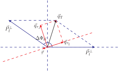
Figure 1: The kinematics on the transverse plane in the laboratory reference frame. $\vec{P}_{t({\bar{t}})}^{\perp}$ stands for the transverse momentum of the (anti-)top quark. $\Delta\Phi_{{t{\bar{t}}}}$ is the azimuthal opening angle between the top and anti-top quarks. $\vec{\tau}$ is a unit reference vector in the transverse plane.

We start this section with the elaboration on the kinematics. As illustrated in Fig. 1, the main concern of this work is on the interplay between a reference unit vector $\vec{\tau}$ and the transverse momentum $\vec{q}_{\mathrm{T}}$ of the ${t{\bar{t}}}$ system. By means of the reference vector $\vec{\tau}$, $\vec{q}_{\mathrm{T}}$ can be decomposed into two parts, the projection component $\vec{q}_{\tau_{\|}}$ and the rejection one $\vec{q}_{\tau_{\perp}}$, i.e.,

$$\vec{q}_{\mathrm{T}}=\vec{q}_{\tau_{\perp}}+\vec{q}_{\tau_{\|}}=q_{\tau_{\perp}}\vec{\tau}\times\vec{n}+q_{\tau_{\|}}\vec{\tau}\,,$$ (2.1)

where $\vec{n}$ is another unit vector pointing to one of beam directions in the laboratory reference frame. In the numeric implementation presented in this paper, the magnitude of the projection $\vec{q}_{\tau_{\|}}$ is of primary interest, which will hereafter be dubbed $q_{\tau}\equiv|\vec{q}_{\tau_{\|}}|$.

The fixed-order calculation on the $q_{\tau}$ spectrum can be realised using the QCD factorisation theorem of [110], that is,

$$\begin{split}\frac{{\rm d}^{5}{\sigma_{{t{\bar{t}}}}}}{{\rm d}M_{t{\bar{t}}}^{2}\,{\rm d}^{2}\vec{P}_{t}^{\perp}\,{\rm d}Y_{t{\bar{t}}}\,{\rm d}q_{\tau}}\,=\;&\sum_{\mathrm{sign}[P_{t}^{z}]}\frac{1}{16s(2\pi)^{6}}\int{\rm d}^{2}\vec{q}_{\mathrm{T}}\,\Theta_{\mathrm{kin}}\,\delta\Big{[}q_{\tau}-|\vec{q}_{\mathrm{T}}\cdot\vec{\tau}|\Big{]}\,\frac{\Sigma_{{t{\bar{t}}}}}{M_{\mathrm{T}}^{t{\bar{t}}}\,|P_{t}^{z}|}\,,\end{split}$$ (2.2)

where $M_{t{\bar{t}}}$ denotes the invariant mass of the ${t{\bar{t}}}$ system, and $s$ is the colliding energy. In this work we will concentrate on $\sqrt{s}=13$ TeV throughout. $Y_{t{\bar{t}}}$ and $M_{\mathrm{T}}^{t{\bar{t}}}$ are for the pseudorapidity and the transverse mass of the ${t{\bar{t}}}$ pair in the laboratory frame (LF), respectively. $P_{t}^{z}$ represents the longitudinal components of the top quark momentum measured from the $z$-direction rest frame ($z$RF) of the ${t{\bar{t}}}$ pair. The $z$RF can be obtained through boosting the LF along one of the beam directions until the longitudinal momentum of the ${t{\bar{t}}}$ pair has been eliminated.

To perform the integral of $\vec{q}_{\mathrm{T}}$ in Eq. (2.2), it is of essence to establish suitable kinematical boundaries to fulfill energy-momentum conservation condition. To this end, we introduce the function $\Theta_{\mathrm{kin}}$ to impose the following constraints,

$$\begin{split}\Theta_{\mathrm{kin}}\,=\,&\Theta\Big{[}\sqrt{s}-M_{\mathrm{T}}^{t{\bar{t}}}-|\vec{q}_{\mathrm{T}}|\Big{]}\,\Theta\Big{[}M_{\mathrm{T}}^{t{\bar{t}}}-m_{\mathrm{T}}^{t}-m_{\mathrm{T}}^{{\bar{t}}}\Big{]}\,\Theta\left[\sinh^{-1}\left(\sqrt{\frac{(M_{t{\bar{t}}}^{2}+s)^{2}}{4\,s\,{M_{\mathrm{T}}^{t{\bar{t}}}}^{2}}-1}\right)-|Y_{t{\bar{t}}}|\right]\,,\end{split}$$ (2.3)

where $\Theta[\dots]$ is the usual Heaviside function. Therein, $m_{\mathrm{T}}^{t}$ and $m_{\mathrm{T}}^{{\bar{t}}}$ are the transverse masses of the top and anti-top quarks in the LF, respectively. Finally, Eq. (2.2) also entails ${\Sigma_{{t{\bar{t}}}}}$, encoding the contributions from all partonic processes, defined as,

$$\begin{split}{\Sigma_{{t{\bar{t}}}}}\,=&\;\sum_{i,j}\int^{1}_{0}\frac{{\rm d}x_{n}}{x_{n}}\,\frac{{\rm d}x_{{\bar{n}}}}{x_{{\bar{n}}}}\,f_{i/N}(x_{n})\,f_{j/\bar{N}}(x_{{\bar{n}}})\,\sum_{r}\,\int\,\prod_{m}^{r}{\rm d}\Phi_{k_{m}}\;(2\pi)^{4}\delta^{4}\left(p_{i}+p_{j}-p_{t}-p_{\bar{t}}-\sum_{m}k_{m}\right)\\ &\;\times\overline{\sum_{\mathrm{hel,col}}}\left|\mathcal{M}(i+j\to t+\bar{t}+X)\right|^{2}\,.\end{split}$$ (2.4)

Here $f_{i/N}(x)$ is the parton distribution function (PDF) for the parton $i$ within the proton $N$ carrying the momentum fraction $x$. ${\rm d}\Phi_{k_{m}}$ characterises the phase space integral of the $m$-th emitted parton, that is,

$$\begin{split}{\rm d}\Phi_{k_{m}}\,\equiv\,\frac{{\rm d}^{4}k_{m}}{(2\pi)^{3}}\,\delta(k_{m}^{2})\,\Theta(k_{m}^{0})\,=\,\frac{1}{2}\;\frac{{\rm d}y_{m}}{2\pi}\;\frac{{\rm d}^{2}\vec{k}_{m}^{\perp}}{(2\pi)^{2}}\,,\end{split}$$ (2.5)

where $y_{m}$ and $\vec{k}_{m}^{\perp}$ indicate the rapidity and transverse momentum of the occurring emission, respectively. $|\mathcal{M}|^{2}$ is the squared transition amplitude for the partonic processes of the indices indicated. Substituting Eq. (2.4) into Eq. (2.2), it is ready to perform the fixed-order calculations of the spectra of $q_{\tau}$. In the vicinity of $q_{\tau}=0$ GeV, however, this perturbative expansion fails to converge, and an asymptotic expansion of ${\rm d}\sigma_{{t{\bar{t}}}}/{\rm d}q_{\tau}$ can be carried out in the small parameter $\lambda_{\tau}\equiv q_{\tau}/M_{t{\bar{t}}}$,

$$\frac{{\rm d}{\sigma_{{t{\bar{t}}}}}}{{\rm d}q_{\tau}}\;\sim\;\sigma^{{t{\bar{t}}}}_{\mathrm{B}}\,\sum_{m,n}\,\left[\frac{\alpha_{s}(M_{t{\bar{t}}})}{4\pi}\right]^{m}\,\left[\underbrace{c^{(0)}_{m,n}\,\frac{\ln^{n}(\lambda_{\tau})}{\lambda_{\tau}}}_{\mathrm{LP}}+\,\underbrace{c^{(1)}_{m,n}\,\ln^{n}(\lambda_{\tau})}_{\mathrm{NLP}}+\,\underbrace{c^{(2)}_{m,n}\,\lambda_{\tau}\ln^{n}(\lambda_{\tau})}_{\mathrm{N}^{2}\mathrm{LP}}+\dots\right]\;,$$ (2.6)

indicating the leading, next-to-leading and next-to-next-to-leading power terms in $\lambda_{\tau}$, labelled LP, NLP, and N²LP, respectively. Therein, $\sigma^{{t{\bar{t}}}}_{\mathrm{B}}$ is the Born level total cross section of the process $pp\to{t{\bar{t}}}+X$, $\alpha_{s}$ denotes the strong coupling constant, and $c^{(k)}_{m,n}$ represents the coefficient for the asymptotic constituent with the superscript $k$ specifying the occurring power. Thus, conventionally, the leading power terms $c^{(0)}_{m,n}\ln^{n}(\lambda_{\tau})/\lambda_{\tau}$ are associated with the most singular behaviors in the low $q_{\tau}$ domain and also the main concern of this work. It is important to note, however, that also the next-to-leading power terms, $c^{(1)}_{m,n}\ln^{n}(\lambda_{\tau})$, are divergent as $\lambda_{\tau}\to 0$.

2.2 Dynamic regions

Based on the strategy of expansion of dynamic regions [78, 79, 80, 81], the asymptotic series of Eq. (2.6) can be interpreted with the aid of a set of regions from the phase space and loop integrals. This work, in particular, will choose the formalism of [81]. We base the definition of our regions on the criterion of domain completeness, i.e. the existence of a set of non-intersecting dynamic regions that cover the whole integration domain. This criterion plays an essential role in consistently extrapolating the expanded integrands from their own convergent domains to the entire integration ranges. Other constraints are also imposed therein, including the regularisation of the expanded integrands and the (at least partial) commutativity amongst the asymptotic expansions. The former case can be fulfilled by introducing the rapidity regulator [111, 107, 109, 96, 97, 98, 99] in implementing the SCET_II formalism [89, 90, 91]. However, for the latter criterion, we assume that all the non-commutative dynamic regions, such as the collinear-plane modes [81], will cancel out in the eventual $q_{\tau}$ spectra. It merits noting that, this ansatz, together with the proposal of [81], has been scrutinised only within the one-loop integrals in the various kinematical limits. We regard their effectiveness on ${t{\bar{t}}}$ hadroproduction as the primary hypothesis in this work. Recent developments on the criteria to implement the region analysis can be found in [112, 113, 114].

As the first application of the domain completeness, we explore the relevant modes for the $\vec{q}_{\tau_{\perp}}$ integral here. From Eq. (2.2), two types of scales will be involved, one of $\mathcal{O}(q_{\tau})$ and the other of $\mathcal{O}(M_{t{\bar{t}}})$. In order to disentangle the influences of those two scales and to also fulfil the constraints of [81], we identify the dynamic regions for the rejection component as follows

$$\mathbf{Isotropic}\textrm{-}\mathbf{recoil}: \;M_{t{\bar{t}}}\gg|\vec{q}_{\tau_{\perp}}|\sim q_{\tau}\,,$$ (2.7)

$$\mathbf{Asymmetric}\textrm{-}\mathbf{recoil}: \;|\vec{q}_{\tau_{\perp}}|\sim M_{t{\bar{t}}}\gg q_{\tau}\,.$$ (2.8)

To precisely separate both regimes and still cover the complete integration range, we introduce the auxiliary boundary $\Lambda_{\tau}$ satisfying $M_{t{\bar{t}}}\gg\Lambda_{\tau}\gg q_{\tau}$, from which the two non-intersecting intervals read $|\vec{q}_{\tau_{\perp}}|\lesssim\Lambda_{\tau}$ and $\Lambda_{\tau}\lesssim|\vec{q}_{\tau_{\perp}}|$. However, as demonstrated in [81], those auxiliary boundary dependences will all drop out after assembling all relevant domains. Their dependence is thus dropped in the following. An analogous analysis is also applied to the phase space integral for the real emissions in Eq. (2.5), which leads to,

$$\mathbf{Soft}:\; \;{y_{m}}\sim 0\,,\quad\quad\quad\quad~{}|\vec{k}_{m}^{\perp}|\sim q_{\tau}\,,$$ (2.9)

$$\mathbf{Beam}\textrm{-}\mathbf{collinear}\textrm{-}n:\, \;{y_{m}}\sim+\ln\lambda_{\tau}\,,\quad\quad|\vec{k}_{m}^{\perp}|\sim q_{\tau}\,,$$ (2.10)

$$\mathbf{Beam}\textrm{-}\mathbf{collinear}\textrm{-}{\bar{n}}:\; \;{y_{m}}\sim-\ln\lambda_{\tau}\,,\quad\quad|\vec{k}_{m}^{\perp}|\sim q_{\tau}\,,$$ (2.11)

$$\mathbf{Jet}\textrm{-}\mathbf{collinear}\textrm{-}{n_{\mathrm{J}}}:\; \;{y_{m}}\sim 0\,,\quad\quad\quad\quad~{}|\vec{k}_{m}^{\perp}|\sim M_{t{\bar{t}}}\,.$$ (2.12)

Therein, the decomposition of the $\vec{k}_{m}^{\perp}$ integration range respects a similar pattern as the $\vec{q}_{\tau_{\perp}}$ case. The rapidity integrals are broken down with respect to the reference points $\pm\Lambda_{y_{m}}$ with the relationship $0\ll\Lambda_{y_{m}}\ll\ln\lambda_{\tau}$, from which three non-overlapping regions emerge, ${y_{m}}\lesssim-\Lambda_{y_{m}}$, $-\Lambda_{y_{m}}\lesssim{y_{m}}\lesssim\Lambda_{y_{m}}$, and $\Lambda_{y_{m}}\lesssim{y_{m}}$. As before, the dependence on the auxiliary boundary $\Lambda_{y_{m}}$ cancels, and we omit it in the following. In addition, please note that in deriving Eq. (2.12) the super-hard-collinear domains ${y_{m}}\sim\pm\ln\lambda_{\tau}$ and $|\vec{k}_{m}^{\perp}|\sim M_{t{\bar{t}}}$ are ignored as they explicitly contradict the energy-momentum conservation condition in Eq. (2.4).

Apart from the above momentum modes, the amplitudes in Eq. (2.4) also contain the loop integrals. A region analysis of this case can proceed in principle in a similar way as for the real emission corrections. However, due to the variability in the offshellness and the varying multiplicity of the external particles, exhausting all relevant circumstances herein is usually more challenging. To this end, this work will utilise momentum regions that can lead to pinched singularities (PS) in a hadron collider process [76, 77, 75, 74, 115, 116], which in general consists of hard, collinear, soft, Coulomb, and Glauber regions. During our calculation, to circumvent the complexity induced by Coulomb singularities, we introduce the lower cutoff upon $M_{t{\bar{t}}}$ in the phase space integral to stay clear of the ${t{\bar{t}}}$ production threshold. In order to cope with the remaining hard, collinear, and soft components, we apply effective field theories, i.e. SCET_II [89, 90, 91] and HQET [92, 93, 94, 95], onto the massless and heavy partons, respectively. Regarding Glauber gluon exchanges, even though their cancellation for inclusive observables has been demonstrated in colour-singlet production in hadronic collisions using a variety of approaches [117, 118, 119, 120], a systematic discussion of their effects on the production of coloured systems, like hadronic ${t{\bar{t}}}$ pair production, is still absent. While leftover soft contributions were observed in ${t{\bar{t}}}$ production in the context of light-cone ordered perturbation theory [121, 122, 123], it nevertheless deserves further confirmation from perturbative QCD, in particular as to whether those soft remnants are eikonalisable or not [124, 125]. In this work, we will follow the approach of [66, 67], and assume the irrelevance of the Glauber contributions. Recent developments in generalizing SCET to encode the Glauber interactions can be found in [126, 127, 128, 124, 129].

We are now ready to summarise the dynamic modes presiding over the virtual and real corrections to the $q_{\tau}$ spectra,

$$\mathbf{Hard}: \quad k_{h}~{}\sim\;M_{t{\bar{t}}}\,\big{[}\mathcal{O}(1),\mathcal{O}(1),\mathcal{O}(1)\big{]}_{n}\,,$$ (2.13)

$$\mathbf{Soft}: \quad k_{s}~{}\sim\;M_{t{\bar{t}}}\,\big{[}\mathcal{O}(\lambda_{\tau}),\mathcal{O}(\lambda_{\tau}),\mathcal{O}(\lambda_{\tau})\big{]}_{n}\,,$$ (2.14)

$$\mathbf{Beam}\textrm{-}\mathbf{collinear}\textrm{-}{n}: \quad k_{c}~{}\sim\;M_{t{\bar{t}}}\,\big{[}\mathcal{O}(1),\mathcal{O}(\lambda_{\tau}^{2}),\mathcal{O}(\lambda_{\tau})\big{]}_{n}\,,$$ (2.15)

$$\mathbf{Beam}\textrm{-}\mathbf{collinear}\textrm{-}{{\bar{n}}}: \quad k_{\bar{c}}~{}\sim\;M_{t{\bar{t}}}\,\big{[}\mathcal{O}(\lambda_{\tau}^{2}),\mathcal{O}(1),\mathcal{O}(\lambda_{\tau})\big{]}_{n}\,,$$ (2.16)

$$\mathbf{Jet}\textrm{-}\mathbf{collinear}\textrm{-}{n_{\mathrm{J}}}: \quad k_{\mathrm{J}}~{}\sim\;M_{t{\bar{t}}}\,\big{[}\mathcal{O}(1),\mathcal{O}(\lambda_{\tau}^{2}),\mathcal{O}(\lambda_{\tau})\big{]}_{n_{\mathrm{J}}}\,.$$ (2.17)

In writing those momentum modes, the light-cone coordinate system has been applied, from which an arbitrary momentum $p^{\mu}$ are decomposed and reforged as

$$p^{\mu}=\frac{p\cdot{\bar{n}}_{k}}{2}n_{k}^{\mu}+\frac{p\cdot n_{k}}{2}{\bar{n}}_{k}^{\mu}+{p}^{\perp,\mu}_{n_{k}}\equiv\frac{p_{{\bar{n}}_{k}}}{2}n_{k}^{\mu}+\frac{p_{n_{k}}}{2}{\bar{n}}_{k}^{\mu}+{p}^{\perp,\mu}_{n_{k}}\equiv\big{[}p_{{\bar{n}}_{k}},p_{n_{k}},{p}_{n_{k}}^{\perp}\big{]}_{n_{k}}.$$ (2.18)

Therein, $n_{k}$ and ${\bar{n}}_{k}$ are two light-like vectors with the normalisation conditions $n_{k}\cdot{\bar{n}}_{k}=2$ and $n^{0}_{k}={\bar{n}}^{0}_{k}=1$. Throughout this paper, we will make use of the symbols $n$ (${\bar{n}}$) and $n_{\mathrm{J}}$ to characterise the positive (negative) beam and jet directions, respectively. In accordance with Eq. (2.12), at least one of the transverse components of the vector $n^{\mu}_{\mathrm{J}}$ should be non-vanishing. In establishing Eqs. (2.14)-(2.17), the offshellnesses of the collinear and soft fluctuations are assigned to be of $\mathcal{O}(\lambda^{2}_{\tau})$ so as to accommodate the projected transverse momentum. The hard-collinear degree of freedom, e.g., $k_{hc}\sim M_{t{\bar{t}}}\,[\mathcal{O}(\lambda_{\tau}),\mathcal{O}(1),\mathcal{O}(\sqrt{\lambda_{\tau}})]_{n}$, is neglected in the analysis as it always results in a scaleless integral for the leading power accuracy investigated in this paper.

By comparison with the calculations on ${\rm d}\sigma_{{t{\bar{t}}}}/{\rm d}q_{\mathrm{T}}$ of [64, 65, 66, 130, 67, 68], in addition to the common pattern of the hard, beam-collinear, and soft regions, this work will also take into account the central jet mode as shown in Eq. (2.17). For the low $q_{\mathrm{T}}$ domain, the subleading nature of the jet region has been demonstrated in [74, 131] by analyzing the powers of the relevant PS surfaces. This conclusion is also expected to hold for our symmetric configuration in Eq. (2.7). Nevertheless, aside from the isotropic recoil, the region expansion strategy in [81] also leads to the asymmetric configuration of Eq. (2.8) participating in the $q_{\tau}$ spectra. In light of the different scaling behaviors in both regions, it is a priori not clear whether the conclusion in [74, 131] derived for the isotropic pattern of Eq. (2.7) is still applicable to the asymmetric configuration of Eq. (2.8). To this end, we will revisit the power rules of all the relevant configurations induced by Eqs. (2.7)-(2.8) and Eqs. (2.13)-(2.17) in the following subsections.

To facilitate our discussion, we categorise the $q_{\tau}$ spectrum according to the number of the embedded jet modes $N_{\mathrm{J}}$, more explicitly,

$$\frac{{\rm d}^{5}{\sigma_{{t{\bar{t}}}}}}{{\rm d}M_{t{\bar{t}}}^{2}\,{\rm d}^{2}\vec{P}_{t}^{\perp}\,{\rm d}Y_{t{\bar{t}}}\,{\rm d}q_{\tau}}\longrightarrow\,\sum_{m=0}^{\infty}\,\frac{{\rm d}^{5}{\sigma_{{t{\bar{t}}}}}}{{\rm d}M_{t{\bar{t}}}^{2}\,{\rm d}^{2}\vec{P}_{t}^{\perp}\,{\rm d}Y_{t{\bar{t}}}\,{\rm d}q_{\tau}}\Bigg{|}_{N_{\mathrm{J}}=m}\,.$$ (2.19)

In Sec. 2.3, we will concentrate on the $N_{\mathrm{J}}=0$ configuration, elaborating on the factorisation properties of the occurring constituents and utilising SCET_II and HQET to determine the power accuracy. Sec. 2.4 will then be devoted to all configurations comprising at least one jet. This discussion will be subdivided into Sec. 2.4.1, examining the $N_{\mathrm{J}}=1$ configuration as an example to present the generic scaling feature in presence of the jet mode, and Sec. 2.4.2, where we move on to the more general situation, the $N_{\mathrm{J}}\geq 2$ contributions, enumerating all the possible scaling behaviors brought about by the various jet momenta present. At last, we will summarise our observations and compare the power prescriptions derived in EFT with those established in [74, 131].

2.3 The case of $N_{\mathrm{J}}=0$

Figure 2: Dynamic regions in the $N_{\mathrm{J}}=0$ configuration. Herein, the black bubbles stand for the hard modes. The red bubble and springs encode the soft fluctuations connecting the heavy partons represented by the black double lines as well as the collinear modes depicted in the blue straight lines.

In this part, we will discuss the dynamic regions contributing to the $N_{\mathrm{J}}=0$ configuration, which comprises the hard, beam-collinear, and soft regions, as exhibited in Eqs. (2.13)-(2.16). As opposed to the beam-collinear and soft regions, which can be assigned to both the phase space and loop integrals, the hard mode is only present in the virtual processes. In this regard, the transverse momentum for the ${t{\bar{t}}}$ system observes only the isotropic pattern in Eq. (2.7), which thus permits us to perform the expansion on the kinematic variables in Eq. (2.2) as follows,

$$P^{z}_{t}\Bigg{|}_{N_{\mathrm{J}}=0} =\;\frac{x_{t}\beta_{t{\bar{t}}}}{\sqrt{1-\beta^{2}_{{t{\bar{t}}}}}}\,m_{t}\,+\mathcal{O}(\lambda_{\tau})\,,$$ (2.20)

where $\beta_{t{\bar{t}}}\equiv\sqrt{1-4m_{t}^{2}/M_{t{\bar{t}}}^{2}}$ with $m_{t}$ denoting the mass of the (anti-)top quark. $x_{t}$ is the cosine of the scattering angle of the top quark in the ${t{\bar{t}}}$ rest frame. Further,

$$M_{\mathrm{T}}^{t{\bar{t}}}\Bigg{|}_{N_{\mathrm{J}}=0} =\;M_{t{\bar{t}}}\,+\mathcal{O}(\lambda_{\tau})\,,$$ (2.21)

and, thus,

$$\Theta_{\mathrm{kin}}\Bigg{|}_{N_{\mathrm{J}}=0} =\;\Theta\left(\sqrt{s}-M_{t{\bar{t}}}^{2}\right)\,\Theta\left(M_{t{\bar{t}}}-2\sqrt{m_{t}^{2}+(\vec{P}^{\perp}_{t})^{2}}\right)\,\Theta\left[\sinh^{-1}\left(\frac{s-M_{t{\bar{t}}}^{2}}{2M_{t{\bar{t}}}\sqrt{s}}\right)-|Y_{t{\bar{t}}}|\right]+\mathcal{O}(\lambda_{\tau})$$

$$\equiv\;\Theta_{\mathrm{kin}}^{(0)}+\mathcal{O}(\lambda_{\tau})\,.$$ (2.22)

Please note, in the results above only the LP contributions are kept. Similarly, in the following, we define the LP term in Eq. (2.3) as $\Theta_{\mathrm{kin}}^{(0)}$ hereafter.

The remaining task is now to expand the partonic convolution function $\Sigma_{{t{\bar{t}}}}$ in line with Eqs. (2.13)-(2.16). This can be achieved by means of the effective field theories, i.e. SCET_II and HQET. Therein, the beam-collinear regions are embodied in terms of the gluon and quark fields, $A_{n(\bar{n})}$ and $\xi_{n(\bar{n})}$ [88, 132, 90, 91] in SCET_II. The soft fluctuations on the heavy (anti-)quark are encoded by the field $h_{v}(\chi_{v})$ from HQET, while those from the incoming gluons and massless quarks are reflected by the fields $A_{s}$ and $q_{s}$ [90, 91] in SCET_II. The hard mode can be taken care of by the effective Hamiltonian $\mathcal{H}_{{t{\bar{t}}}}^{\mathrm{eff}}$ [51], which consists of products of Wilson coefficients and the corresponding field operators.

Up to LP, the interactions in the individual momentum regions are governed by the effective Lagrangians [89, 90, 91, 95],

$$\mathcal{L}_{n}= \;\bar{\xi}_{n}\Big{(}in\cdot D_{n}+i\not{D}_{n\perp}\frac{1}{i{\bar{n}}\cdot D_{n}}i\not{D}_{n\perp}\Big{)}\frac{\not{{\bar{n}}}}{2}\xi_{n}-\frac{1}{2}\mathbf{Tr}\Big{[}F^{\mu\nu}_{n}F_{\mu\nu}^{n}\Big{]}\,,$$ (2.23)

$$\mathcal{L}_{s}= \;-\frac{1}{2}\mathbf{Tr}\Big{[}F^{\mu\nu}_{\text{s}}F_{\mu\nu}^{\text{s}}\Big{]}+\bar{q}_{\text{s}}i\not{D}_{\text{s}}q_{\text{s}}\,,$$ (2.24)

$$\mathcal{L}_{v}= \;\bar{h}_{v}\left(i\partial\cdot v\right)h_{v}+\bar{\chi}_{v}\left(i\partial\cdot v\right)\chi_{v}\,,$$ (2.25)

where $D^{\mu}_{n(s)}\equiv\partial^{\mu}-ig_{s}A^{\mu}_{n(s)}$ and $F_{n(s)}^{\mu\nu}\equiv(i/g_{s})[D^{\mu}_{n(s)},D^{\nu}_{n(s)}]$ stand for the covariant derivative and the field strength tensor for the collinear (soft) fields $A^{\mu}_{n(s)}$, respectively. The Lagrangian $\mathcal{L}_{{\bar{n}}}$ can be obtained by exchanging $n\leftrightarrow{\bar{n}}$ in $\mathcal{L}_{n}$. In deriving Eqs. (2.23)-(2.25), the decoupling transformations [82, 58] have already been performed to strip the soft particle of the collinear and heavy partons. As a result, the (anti-)top quark is free of any interactions at this point, while the collinear partons only communicate with themselves. The LP contribution of $\Sigma_{{t{\bar{t}}}}$ can be found through assembling the amplitudes induced by $\mathcal{H}_{{t{\bar{t}}}}^{\mathrm{eff}}$ and the effective Lagrangians in Eqs. (2.23)-(2.25), and we follow the scheme of [51, 65] to construct the hard contributions. In light of the rapidity divergences arising from the soft and collinear integrals, the exponential regulator proposed in [98, 99] is applied throughout. Finally, the decoupling nature of the Lagrangians in Eqs. (2.23)-(2.25) allows us to rewrite $\Sigma_{{t{\bar{t}}}}$ as,

$$\Sigma_{{t{\bar{t}}}}\Bigg{|}_{N_{\mathrm{J}}=0}= \;\frac{8\pi^{2}}{M_{t{\bar{t}}}^{2}}\,\sum_{\kappa}\,\int{{\rm d}^{2}\vec{b}_{\mathrm{T}}}\,\exp\left(\mathrm{i}\,\vec{b}_{\mathrm{T}}\cdot\vec{q}_{\mathrm{T}}\right)\,\widetilde{\Sigma}_{{t{\bar{t}}}}^{[\kappa]}(\vec{b}_{\mathrm{T}},M_{t{\bar{t}}},\beta_{t{\bar{t}}},x_{t},Y_{t{\bar{t}}},\mu,\nu)\,\mathcal{W}_{t}\,\mathcal{W}_{{\bar{t}}}\,,$$ (2.26)

where $\vec{b}_{\mathrm{T}}$ is the impact parameter introduced during the Fourier transformation. $\Sigma_{{t{\bar{t}}}}$ includes the contributions from all channels $\kappa\in\{g_{n}g_{{\bar{n}}},q^{i}_{n}\bar{q}^{j}_{{\bar{n}}},q^{i}_{{\bar{n}}}\bar{q}^{j}_{n}\}$, with $i,j\in\{u,d,c,s,b\}$ indicating the flavour of the quark field. $\mu$ and $\nu$ are the scales associated with the virtuality and rapidity renormalisations, respectively. Finally, $\mathcal{W}_{t}$ and $\mathcal{W}_{{\bar{t}}}$ are the heavy parton correlation functions,

$$\mathcal{W}_{t}= \frac{1}{4m_{t}N_{c}}\,\mathbf{Tr}\,\langle 0|{h}_{v_{t}}\left(0\right)|t\rangle\langle t|\bar{h}_{v_{t}}\left(0\right)\frac{1+\not{v}_{t}}{2}|0\rangle=1\,,$$ (2.27)

$$\mathcal{W}_{{\bar{t}}}= -\frac{1}{4m_{t}N_{c}}\,\mathbf{Tr}\,\langle 0|\bar{\chi}_{v_{\bar{t}}}\left(0\right)|{\bar{t}}\rangle\langle{\bar{t}}|\frac{1-\not{v}_{{\bar{t}}}}{2}{\chi}_{v_{{\bar{t}}}}\left(0\right)|0\rangle=1\,,$$ (2.28)

where $N_{c}=3$ is the colour factor. $v_{t({\bar{t}})}$ is the velocity of the (anti)top quark in the rest frame of the ${t{\bar{t}}}$ system. Considering that the (anti-)top quark up to the LP accuracy amounts to a free particle, the correlation functions $\mathcal{W}_{t({\bar{t}})}$ will never receive any perturbative corrections. Therefore, in the second steps of Eqs. (2.27)-(2.28), we evaluate them using the tree-level expressions.

Apart from the correlation function $\mathcal{W}_{t(\bar{t})}$, Eq. (2.26) entails the partonic cross sections $\widetilde{\Sigma}_{{t{\bar{t}}}}^{[\kappa]}$ as well, which are built by suitably combining beam-collinear, soft and hard functions,

$$\widetilde{\Sigma}_{{t{\bar{t}}}}^{[q^{i}_{n}\bar{q}^{j}_{{\bar{n}}}]}(\vec{b}_{\mathrm{T}},M_{t{\bar{t}}},\beta_{t{\bar{t}}},x_{t},Y_{t{\bar{t}}},\mu,\nu)= \left(\frac{1}{2N_{c}}\right)^{2}\,\mathcal{B}_{n}^{[q_{n}^{i}]}(\eta_{n},b_{\mathrm{T}},\mu,\nu)\,\mathcal{B}_{{\bar{n}}}^{[\bar{q}_{n}^{j}]}(\eta_{{\bar{n}}},b_{\mathrm{T}},\mu,\nu)\,$$

$$\times\,\sum_{\alpha,\beta}\left\{\mathcal{H}_{\alpha\beta}^{[q^{i}_{n}\bar{q}^{j}_{{\bar{n}}}]}(M_{t{\bar{t}}},\beta_{t{\bar{t}}},x_{t},\mu)\,\mathcal{S}^{\alpha\beta}_{[q_{n}\bar{q}_{{\bar{n}}}]}(\vec{b}_{\mathrm{T}},\mu,\nu)\right\}\,,$$ (2.29)

$$\widetilde{\Sigma}_{{t{\bar{t}}}}^{[g_{n}g_{{\bar{n}}}]}(\vec{b}_{\mathrm{T}},M_{t{\bar{t}}},\beta_{t{\bar{t}}},x_{t},Y_{t{\bar{t}}},\mu,\nu)= \left(\frac{1}{N^{2}_{c}-1}\right)^{2}\,\sum_{\begin{subarray}{c}\alpha,\beta,{{h_{n}^{\phantom{\prime}}}},{{h_{n}^{\prime}}},{{h_{\bar{n}}^{\phantom{\prime}}}},{{h_{\bar{n}}^{\prime}}}\end{subarray}}\left\{\mathcal{B}^{[g_{{\bar{n}}}]}_{{\bar{n}},{{h_{\bar{n}}^{\prime}}}{{h_{\bar{n}}^{\phantom{\prime}}}}}(\eta_{{\bar{n}}},\vec{b}_{\mathrm{T}},\mu,\nu)\,\mathcal{B}^{[g_{n}]}_{n,{{h_{n}^{\prime}}}{{h_{n}^{\phantom{\prime}}}}}(\eta_{n},\vec{b}_{\mathrm{T}},\mu,\nu)\,\right.$$

$$\left.\times\,\mathcal{H}_{\alpha\beta;{{{h_{\bar{n}}^{\prime}}}}{{h_{\bar{n}}^{\phantom{\prime}}}};{{h_{n}^{\prime}}}{{h_{n}^{\phantom{\prime}}}}}^{[g_{n}g_{{\bar{n}}}]}(M_{t{\bar{t}}},\beta_{t{\bar{t}}},x_{t},\mu)\,\mathcal{S}^{\alpha\beta}_{[g_{n}g_{{\bar{n}}}]}(\vec{b}_{\mathrm{T}},\mu,\nu)\right\}\,,$$ (2.30)

where the momentum fractions $\eta_{n}$ and $\eta_{{\bar{n}}}$ are defined as $\eta_{n}=M_{t{\bar{t}}}\,e^{Y_{t{\bar{t}}}}/\sqrt{s}$ and $\eta_{{\bar{n}}}=M_{t{\bar{t}}}\,e^{-Y_{t{\bar{t}}}}/\sqrt{s}$, respectively. The expression for $\widetilde{\Sigma}_{{t{\bar{t}}}}^{[q^{i}_{{\bar{n}}}\bar{q}^{j}_{{n}}]}$ can be derived by exchanging the labels $n\leftrightarrow{\bar{n}}$.

$\mathcal{H}_{\alpha\beta}^{[q^{i}_{n}\bar{q}^{j}_{{\bar{n}}}]}$ and $\mathcal{H}_{\alpha\beta;{{h_{\bar{n}}^{\prime}}}{{h_{\bar{n}}^{\phantom{\prime}}}};{{h_{n}^{\prime}}}{{h_{n}^{\phantom{\prime}}}}}^{[g_{n}g_{{\bar{n}}}]}$ are the hard functions for the quark and gluon initiated processes, respectively. The indices $\alpha$ and $\beta$ label the colour states to track the full colour correlation between the hard and the soft functions detailed below. Similarly, the ${{h_{n}^{\phantom{\prime}}}}$, ${{h_{n}^{\prime}}}$, ${{h_{\bar{n}}^{\phantom{\prime}}}}$, and ${{h_{\bar{n}}^{\prime}}}$ denote the polarisation states of the incoming gluons to capture all off-diagonal correlation effects of the beam-collinear and hard functions. Please note, that the beam-hard function correlation for massless quarks is devoid of off-diagonal contributions. The hard functions now account for the LP contributions from the deep off-shell region in Eq. (2.13). Their expressions read [51, 65],

$$\mathcal{H}_{\alpha\beta}^{[q^{i}_{n}\bar{q}^{j}_{{\bar{n}}}]}(M_{t{\bar{t}}},\beta_{t{\bar{t}}},x_{t},\mu)= \sum_{\alpha^{\prime},\beta^{\prime}}\,\Big{(}\mathcal{Z}^{h,{\alpha^{\prime}\alpha}}_{[{q_{n}\bar{q}_{{\bar{n}}}}]}\Big{)}^{*}\,\mathcal{Z}^{h,{\beta^{\prime}\beta}}_{[{q_{n}\bar{q}_{{\bar{n}}}}]}\,{\sum_{\{a,a^{\prime},h\}}}\,c_{a^{\prime}_{1}a^{\prime}_{2}a^{\prime}_{3}a^{\prime}_{4}}^{qq,(\alpha^{\prime})}\,\left[c_{a_{1}a_{2}a_{3}a_{4}}^{qq,(\beta^{\prime})}\right]^{*}\,$$

$$\quad\times\mathcal{M}^{*}(\bar{q}^{a^{\prime}_{1}h_{1}^{\phantom{\prime}}}_{{\bar{n}},j}{q}^{a^{\prime}_{2}h_{2}^{\phantom{\prime}}}_{n,i}\to t_{a^{\prime}_{3}h_{3}^{\phantom{\prime}}}\bar{t}_{a^{\prime}_{4}h_{4}^{\phantom{\prime}}})\,\mathcal{M}(\bar{q}^{a_{1}h_{1}}_{{\bar{n}},j}{q}^{a_{2}h_{2}}_{n,i}\to t_{a_{3}h_{3}}\bar{t}_{a_{4}h_{4}})\,,$$ (2.31)

$$\mathcal{H}_{\alpha\beta;h^{\prime}_{1}h_{1};h^{\prime}_{2}h_{2}}^{[g_{n}g_{{\bar{n}}}]}(M_{t{\bar{t}}},\beta_{t{\bar{t}}},x_{t},\mu)= \sum_{\alpha^{\prime},\beta^{\prime}}\,\Big{(}\mathcal{Z}^{h,{\alpha^{\prime}\alpha}}_{[{g_{n}g_{{\bar{n}}}}]}\Big{)}^{*}\,\mathcal{Z}^{h,{\beta^{\prime}\beta}}_{[{g_{n}g_{{\bar{n}}}}]}\,{\sum_{\{a,a^{\prime}\},h_{3},h_{4}}}\,c_{a^{\prime}_{1}a^{\prime}_{2}a^{\prime}_{3}a^{\prime}_{4}}^{gg,(\alpha^{\prime})}\,\left[c_{a_{1}a_{2}a_{3}a_{4}}^{gg,(\beta^{\prime})}\right]^{*}\,$$

$$\quad\times\mathcal{M}^{*}(g^{a^{\prime}_{1}h^{\prime}_{1}}_{{\bar{n}}}g^{a^{\prime}_{2}h^{\prime}_{2}}_{n}\to t_{a^{\prime}_{3}h_{3}^{\phantom{\prime}}}\bar{t}_{a^{\prime}_{4}h_{4}^{\phantom{\prime}}})\,\mathcal{M}(g^{a_{1}h_{1}}_{{\bar{n}}}g^{a_{2}h_{2}}_{n}\to t_{a_{3}h_{3}}\bar{t}_{a_{4}h_{4}})$$ (2.32)

where $\mathcal{M}$ denotes the amplitude for the partonic process $\bar{q}q\to{t{\bar{t}}}$ or $gg\to{t{\bar{t}}}$. Therein, the variables $a_{i}$$(i=1,\dots,4)$ are introduced for the colour states of the individual external particles. In particular, every $a_{i}$ runs over the set $\{1,\dots,3\}$ for quarks and anti-quarks, and $\{1,\dots,8\}$ for gluons. Also, to facilitate our calculation, the orthonormal colour bases $c^{qq}_{\{a\}}$ and $c^{gg}_{\{a\}}$ [133] are exploited in Eqs. (2.31)-(2.32), more explicitly,

$$c^{qq,(1)}_{a_{1}a_{2}a_{3}a_{4}} =\frac{1}{3}\,\delta_{a_{1}a_{2}}\delta_{a_{3}a_{4}}\,,\;\;c^{qq,(2)}_{a_{1}a_{2}a_{3}a_{4}}=\frac{1}{\sqrt{2}}\sum_{c}T^{c}_{a_{1}a_{2}}T^{c}_{a_{3}a_{4}}\,,$$ (2.33)

$$c^{gg,(1)}_{a_{1}a_{2}a_{3}a_{4}} =\frac{1}{2\sqrt{6}}\,\delta_{a_{1}a_{2}}\delta_{a_{3}a_{4}}\,,\;\;c^{gg,(2)}_{a_{1}a_{2}a_{3}a_{4}}=\frac{i}{2\sqrt{3}}\,\sum_{c}f^{a_{1}ca_{2}}T^{c}_{a_{3}a_{4}}\,,\;\;c^{gg,(3)}_{a_{1}a_{2}a_{3}a_{4}}=\frac{1}{2}\sqrt{\frac{3}{5}}\sum_{c}d^{a_{1}ca_{2}}T^{c}_{a_{3}a_{4}}\,,$$ (2.34)

where $T^{c}_{ab}$ stands for the generator in the fundamental representation of the SU$(3)$ group. $f_{abc}$ and $d_{abc}$ mark the antisymmetric and symmetric structure constants for the SU$(3)$ group, respectively. As alluded to above, in calculating the hard functions, due to the absence of spin-correlations for external quarks, we take the sum over all the helicity configurations for the quark channel, while, to capture the non-diagonal gluon polarisation effects, the explicit dependence of $\mathcal{H}_{\alpha\beta;h^{\prime}_{1}h_{1};h^{\prime}_{2}h_{2}}^{[g_{n}g_{{\bar{n}}}]}$ on the gluon helicities is retained.

To evaluate the amplitudes in Eqs. (2.31)-(2.32), we make use of the on-shell prescription to renormalise the top quark mass and the $n_{f}=5$ active flavor scheme to handle the UV divergences from the strong coupling. The remaining singularities are of infrared origin, and are subtracted by means of $\mathcal{Z}^{h}_{[{g_{n}g_{{\bar{n}}}}]}$ and $\mathcal{Z}^{h}_{[{q_{n}\bar{q}_{{\bar{n}}}}]}$ following the method in [134]. Up to NLO, the amplitudes of all the helicity and colour configurations can be extracted from R ECOLA  [135, 136]. The NNLO results are more involved, and in consequence we will only address their logarithmic parts in this work. For reference, grid-based NNLO results can be found in [137], and the progress towards the full analytic evaluations is discussed in [138, 139, 140].

$\mathcal{B}_{n}^{[q_{n}^{i}]}$ and $\mathcal{B}^{[g_{n}]}_{n,h^{\prime}h}$ are the quark and gluon beam functions, respectively, collecting the contributions from the region in Eq. (2.15). Their definitions in the exponential regularisation scheme are [98, 141, 142],

$$\mathcal{B}_{n}^{[q_{n}^{i}]}(\eta_{n},b_{\mathrm{T}},\mu,\nu)= \;\mathcal{Z}^{c}_{[q_{n}]}\Big{(}\mathcal{Z}^{cs}_{[q_{n}]}\Big{)}^{-1}\,\lim_{\delta\to 0^{+}}\,\int\frac{{\rm d}b_{n}}{4\pi}\,\exp\left(\frac{-\mathrm{i}\eta_{n}b_{n}P_{{\bar{n}}}}{2}\right)\,$$ (2.35)

$$\times\mathbf{Tr}\,\langle N(P)|\overline{\xi}^{i}_{n}W_{n}(-{ib_{0}\delta},-{ib_{0}\delta}+b_{n},\vec{b}_{\mathrm{T}})\frac{\not{{\bar{n}}}}{2}W^{\dagger}_{n}{\xi}^{i}_{n}(0)|N(P)\rangle\bigg{|}_{\delta=\frac{1}{\nu}}\,,$$

$$\mathcal{B}^{[g_{n}]}_{n,h^{\prime}h}(\eta_{n},\vec{b}_{\mathrm{T}},\mu,\nu)= \;\mathcal{Z}^{c}_{[g_{n}]}\Big{(}{\mathcal{Z}^{cs}_{[g_{n}]}}\Big{)}^{-1}\,\lim_{\delta\to 0^{+}}\,\int\frac{{\rm d}b_{n}}{4\pi}\,\exp\left(\frac{-\mathrm{i}\eta_{n}b_{n}P_{{\bar{n}}}}{2}\right)\,$$ (2.36)

$$\times\mathbf{Tr}\,\langle N(P)|\mathcal{A}^{\perp}_{n,\rho}(-{ib_{0}\delta},-{ib_{0}\delta}+b_{n},\vec{b}_{\mathrm{T}})\,\epsilon^{\rho}_{n,h^{\prime}}\,\left(-\eta_{n}P_{{\bar{n}}}\right)\,\epsilon^{\sigma*}_{n,h}\,\mathcal{A}^{\perp}_{n,\sigma}(0)|N(P)\rangle\bigg{|}_{\delta=\frac{1}{\nu}}\,,$$

where $\mathcal{Z}^{c}_{[q_{n}]([g_{n}])}$ is the renormalisation constant for the quark (gluon) beam function in the $\overline{\mathrm{MS}}$ scheme. $\mathcal{Z}^{cs}_{[q_{n}]}$ and $\mathcal{Z}^{cs}_{[g_{n}]}$ represent the ensuing zero-bin subtrahend to remove the soft-collinear overlapping terms. $\delta$ is the exponential regulator suggested in [98], accompanied by the constant $b_{0}\equiv 2\exp(-\gamma_{\mathrm{E}})$. $\mu$ and $\nu$ are the scales associated with the virtuality and rapidity renormalisations, respectively. Within the matrix elements, ${\xi}^{i}_{n}$ denotes the collinear quark field of the flavour $i$ given in Eq. (2.23). $\mathcal{A}_{n,\perp}^{\mu}\equiv\frac{1}{g_{s}}\,W_{n}^{\dagger}(iD_{n,\perp}^{\mu}W_{n})$ signifies the gauge invariant building block for the gluon field with $W_{n}$ denoting the collinear Wilson line [132]. Finally, $P$ is the momentum carried by the initial proton with $P_{{\bar{n}}}=P\cdot{\bar{n}}$ being the largest light-cone component. The anti-quark beam function $\mathcal{B}_{n}^{[\bar{q}_{i}]}$ and those for the ${\bar{n}}$ direction can be obtained by adjusting the labels and fields in Eqs. (2.35)-(2.36) appropriately.

Comparing with the quark beam function, the gluon case possesses extra indices, ${{h_{n}^{\phantom{\prime}}}},{{h_{n}^{\prime}}}\in\{+,-\}$, to characterise its intrinsic polarisation effects [73]. In this work, the following helicity basis is adopted,

$$\epsilon^{\mu}_{n,\pm}\equiv\left\{0,\frac{\mp 1}{\sqrt{2}},\frac{-\mathrm{i}}{\sqrt{2}},0\right\}\,,\qquad\epsilon^{\mu}_{{\bar{n}},\pm}\equiv\left\{0,\frac{\pm 1}{\sqrt{2}},\frac{-\mathrm{i}}{\sqrt{2}},0\right\}\,.$$ (2.37)

In principle, the representations of the helicity polarisation states $\epsilon^{\mu}_{n,\pm}$ are not unique. Nevertheless, in order to avoid the appearance of an unphysical phase factor in the cross section, the helicity space utilised in the beam sector must synchronise with the one used for the hard function in Eq. (2.30). In our case, since we use R ECOLA to extract the hard function, Eq. (2.37) is subject to the choice adopted in this program. The quark beam function is known to N³LO accuracy [143, 144], while for the gluon case only the helicity-conserving components $\mathcal{B}_{++}^{[g_{n({\bar{n}})}]}$ and $\mathcal{B}_{--}^{[g_{n({\bar{n}})}]}$ are known to this order [143]. The helicity-flip components $\mathcal{B}_{+-}^{[g_{n({\bar{n}})}]}$ and $\mathcal{B}_{-+}^{[g_{n({\bar{n}})}]}$ are only known to N²LO [142, 145, 146].

Finally, $\mathcal{S}^{\alpha\beta}_{[q_{n}\bar{q}_{{\bar{n}}}]}$ is the soft function and covers the wide angle domain in Eq. (2.14). Its LP expression is,

$$\mathcal{S}^{\alpha\beta}_{[q_{n}\bar{q}_{{\bar{n}}}]}(\vec{b}_{\mathrm{T}},\mu,\nu)$$

$$= \;\sum_{\alpha^{\prime},\beta^{\prime}}\,\Big{(}\mathcal{Z}^{s,{\alpha\alpha^{\prime}}}_{[q_{n}\bar{q}_{{\bar{n}}}]}\Big{)}^{*}\,\mathcal{Z}^{s,\beta\beta^{\prime}}_{[q_{n}\bar{q}_{{\bar{n}}}]}\,\sum_{\{a,a^{\prime},b\}}\,\lim_{\delta\to 0^{+}}\,\left[c_{a^{\prime}_{1}a^{\prime}_{2}a^{\prime}_{3}a^{\prime}_{4}}^{qq,(\alpha^{\prime})}\right]^{*}\,c_{a_{1}a_{2}a_{3}a_{4}}^{qq,(\beta^{\prime})}\,$$ (2.38)

$$\times\langle 0|\Big{[}\overline{Y}^{\dagger}_{n,b_{2}^{\phantom{\prime}}a^{\prime}_{2}}\overline{Y}_{{\bar{n}},a^{\prime}_{1}b_{1}^{\phantom{\prime}}}Y^{\dagger}_{v_{{\bar{t}}},b_{4}^{\phantom{\prime}}a^{\prime}_{4}}\,Y_{v_{t},a^{\prime}_{3}b_{3}^{\phantom{\prime}}}\Big{]}(-{ib_{0}\delta},-{ib_{0}\delta},\vec{b}_{\mathrm{T}})\,\Big{[}\overline{Y}^{\dagger}_{{\bar{n}},b_{1}a_{1}}\overline{Y}_{n,a_{2}b_{2}}Y^{\dagger}_{v_{t},b_{3}a_{3}}Y_{v_{{\bar{t}}},a_{4}b_{4}}\Big{]}(0)|0\rangle\,\bigg{|}_{\delta=\frac{1}{\nu}}\,,$$

$$\mathcal{S}^{\alpha\beta}_{[g_{n}g_{{\bar{n}}}]}(\vec{b}_{\mathrm{T}},\mu,\nu)$$

$$= \;\sum_{\alpha^{\prime},\beta^{\prime}}\,\Big{(}\mathcal{Z}^{s,{\alpha\alpha^{\prime}}}_{[gg]}\Big{)}^{*}\,\mathcal{Z}^{s,{\beta\beta^{\prime}}}_{[gg]}\,\sum_{\{a,a^{\prime},b\}}\,\lim_{\delta\to 0^{+}}\,\,\left[c_{a^{\prime}_{1}a^{\prime}_{2}a^{\prime}_{3}a^{\prime}_{4}}^{gg,(\alpha^{\prime})}\right]^{*}\,c_{a_{1}a_{2}a_{3}a_{4}}^{gg,(\beta^{\prime})}$$ (2.39)

$$\times\langle 0|\Big{[}\overline{\mathcal{Y}}^{\dagger}_{n,b_{2}^{\phantom{\prime}}a^{\prime}_{2}}\overline{\mathcal{Y}}_{{\bar{n}},a^{\prime}_{1}b_{1}^{\phantom{\prime}}}Y^{\dagger}_{v_{{\bar{t}}},b_{4}^{\phantom{\prime}}a^{\prime}_{4}}\,Y_{v_{t},a^{\prime}_{3}b_{3}^{\phantom{\prime}}}\Big{]}(-{ib_{0}\delta},-{ib_{0}\delta},\vec{b}_{\mathrm{T}})\,\Big{[}\overline{\mathcal{Y}}^{\dagger}_{{\bar{n}},b_{1}a_{1}}\overline{\mathcal{Y}}_{n,a_{2}b_{2}}Y^{\dagger}_{v_{t},b_{3}a_{3}}Y_{v_{{\bar{t}}},a_{4}b_{4}}\Big{]}(0)|0\rangle\,\bigg{|}_{\delta=\frac{1}{\nu}}\;,$$

where $\mathcal{Z}^{s}_{[q_{n}\bar{q}_{{\bar{n}}}]}$ and $\mathcal{Z}^{s}_{[gg]}$ are the renormalisation constants of the soft function in the $\overline{\text{MS}}$ scheme. Again, $\delta$ denotes the rapidity regulator [98, 99], and the $c_{\{a\}}^{qq(gg)}$ are the colour coefficients defined in Eqs. (2.33)-(2.34). $\overline{Y}_{n({\bar{n}})}$ and $\overline{\mathcal{Y}}_{n({\bar{n}})}$ describe the incoming soft Wilson lines for the (anti-)quark and gluon fields, respectively, while the $Y_{v_{t}(v_{{\bar{t}}})}$ are the outgoing soft Wilson lines of the (anti-)top quark. Their specific expressions have been summarised in [133]. Even though the azimuthally averaged soft functions have been computed up to N²LO [64, 65, 147] recently, the azimuthally resolved soft functions, as displayed in Eqs. (2.38)-(2.39), are not yet available in the context of effective field theories. The relevant function at this point is the soft correlation factor defined in [66, 148] which is derived in the generalised $q_{\mathrm{T}}$ resummation framework of [131, 100]. Nevertheless, in this paper, aiming at a self-consistent and independent study, we will revisit the soft interactions in the EFT including the exponential rapidity regulator [98] at NLO accuracy. In Sec. 2.5, we will explicitly calculate the rapidity and virtuality associated divergences originating from the soft sector defined in Eqs. (2.38)-(2.39) and utilise them to examine the consistency condition required by the factorisation of Eqs. (2.29-2.30), providing a powerful test of its validity. Moreover, regarding the finite contributions in the soft function, we will present a comparison between our results and those obtained in [66, 148].

Now we can consider the differential cross section in Eq. (2.2) with the reduced kinematic variables of Eqs. (2.20)-(2.3) as well as the expanded partonic contributions in Eq. (2.26). We begin by disentangling the Fourier integrals in Eq. (2.26) with the help of the reference vector $\vec{\tau}$, using the different scaling behaviours of the components of the vector $\vec{b}_{\mathrm{T}}$ (or correspondingly, $\vec{q}_{\mathrm{T}}$),

$$\Sigma_{{t{\bar{t}}}}\Bigg{|}_{N_{\mathrm{J}}=0}\propto\,\sum_{\kappa}\int^{\infty}_{-\infty}{\rm d}b_{\tau_{\|}}\exp\left(\mathrm{i}\,{q}_{\tau_{\|}}b_{\tau_{\|}}\right)\,\int^{\infty}_{-\infty}{\rm d}b_{\tau_{\perp}}\exp\left(\mathrm{i}\,{q}_{\tau_{\perp}}b_{\tau_{\perp}}\right)\,\widetilde{\Sigma}_{{t{\bar{t}}}}^{[\kappa]}(\vec{b}_{\mathrm{T}},M_{t{\bar{t}}},\beta_{t{\bar{t}}},x_{t},Y_{t{\bar{t}}},\mu,\nu)+\dots\,,$$ (2.40)

where in analogy to the case in Fig. 1, we apply the relationships,

$$\vec{b}_{\mathrm{T}}=\vec{b}_{\tau_{\perp}}+\vec{b}_{\tau_{\|}}=b_{\tau_{\perp}}\vec{\tau}\times\vec{n}+b_{\tau_{\|}}\vec{\tau}\,,\quad\vec{q}_{\mathrm{T}}=\vec{q}_{\tau_{\perp}}+\vec{q}_{\tau_{\|}}=q_{\tau_{\perp}}\vec{\tau}\times\vec{n}+q_{\tau_{\|}}\vec{\tau}\,.$$ (2.41)

Substituting the separated expression in Eq. (2.40) into Eq. (2.2) yields,

$$\frac{{\rm d}^{5}{\sigma_{{t{\bar{t}}}}}}{{\rm d}M_{t{\bar{t}}}^{2}\,{\rm d}^{2}\vec{P}_{t}^{\perp}\,{\rm d}Y_{t{\bar{t}}}\,{\rm d}q_{\tau}}\Bigg{|}_{N_{\mathrm{J}}=0}\propto \,\sum_{\kappa}\int^{\infty}_{-\infty}{\rm d}b_{\tau_{\|}}\,\int^{\infty}_{-\infty}\,{\rm d}q_{\tau_{\|}}\,\delta(q_{\tau}-|q_{\tau_{\|}}|)\,\exp\left(\mathrm{i}\,{q}_{\tau_{\|}}b_{\tau_{\|}}\right)\,$$ (2.42)

$$\times\int^{\infty}_{-\infty}{\rm d}b_{\tau_{\perp}}\,\widetilde{\Sigma}_{{t{\bar{t}}}}^{[\kappa]}(\vec{b}_{\mathrm{T}},M_{t{\bar{t}}},\beta_{t{\bar{t}}},x_{t},Y_{t{\bar{t}}},\mu,\nu)\,$$

$$\times\int^{\infty}_{-\infty}\,{\rm d}q_{\tau_{\perp}}\,\exp\left(\mathrm{i}\,{q}_{\tau_{\perp}}b_{\tau_{\perp}}\right)+\dots\,,$$

where the variables that are independent of $\vec{b}_{\mathrm{T}}$ or $\vec{q}_{\mathrm{T}}$ are omitted for simplicity. In comparison to Eq. (2.2), one of the main differences in Eq. (2.42) resides in the absence of the boundaries on the $q_{\tau_{\perp}}$ integral, which is a consequence of the $\vec{q}_{\mathrm{T}}$ independence in the expanded function $\Theta_{\mathrm{kin}}^{(0)}$ of Eq. (2.3). In this way, the integral over $q_{\tau_{\perp}}$ in the third line of Eq. (2.42) can be completed before the inverse Fourier transformation, thereby leading to the Dirac delta function $\delta(b_{\tau_{\perp}})$. The integration over $b_{\tau_{\perp}}$ is then straightforward, reducing the $\vec{b}_{\mathrm{T}}$ dependence of $\widetilde{\Sigma}_{{t{\bar{t}}}}$ to a dependence on $\vec{b}_{\tau_{\|}}$ only. This leaves the integrals over $b_{\tau_{\|}}$ and $q_{\tau_{\|}}$. The evaluation on the latter is immediate via the function $\delta(q_{\tau}-|q_{\tau_{\|}}|)$ in the first line of Eq. (2.42), eliminating the imaginary part of $\exp(\mathrm{i}\,{q}_{\tau_{\|}}b_{\tau_{\|}})$. The integration over $b_{\tau_{\|}}$, finally, is less straightforward to perform, and we turn to the numeric solutions in Sec. 4.

To summarise, specifying the kinematic factors in Eq. (2.42), we are able to establish the LP contribution from the $N_{\mathrm{J}}=0$ configuration,

$$\frac{{\rm d}^{5}{\sigma_{{t{\bar{t}}}}}}{{\rm d}M_{t{\bar{t}}}^{2}\,{\rm d}^{2}\vec{P}_{t}^{\perp}\,{\rm d}Y_{t{\bar{t}}}\,{\rm d}q_{\tau}}\Bigg{|}_{N_{\mathrm{J}}=0}=\sum_{\mathrm{sign}[x_{t}]}\frac{\Theta_{\mathrm{kin}}^{(0)}}{16\pi^{3}\,\beta_{t{\bar{t}}}\,|x_{t}|\,M^{4}_{{t{\bar{t}}}}\,s}\,\sum_{\kappa}\int^{\infty}_{-\infty} {\rm d}{b}_{\tau_{\|}}\,\cos\left({b}_{\tau_{\|}}{q}_{\tau}\right)\,$$ (2.43)

$$\times\widetilde{\Sigma}_{{t{\bar{t}}}}^{[\kappa]}(b_{\tau_{\|}}\vec{\tau},M_{t{\bar{t}}},\beta_{t{\bar{t}}},x_{t},Y_{t{\bar{t}}},\mu,\nu)\,,$$

where the index $\kappa$ runs over $\{g_{n}g_{{\bar{n}}},q^{i}_{n}\bar{q}^{j}_{{\bar{n}}},q^{i}_{{\bar{n}}}\bar{q}^{j}_{n}\}$ as before. $\Theta_{\mathrm{kin}}^{(0)}$ imposes the kinematic constraints as defined in Eq. (2.20), and the $\widetilde{\Sigma}_{{t{\bar{t}}}}$ are the contributions of the individual partonic processes, as presented in Eqs. (2.29)-(2.30).

It should be stressed that the result in Eq. (2.43) and the factorisation in Eqs. (2.29-2.30) are subject to the absence of other sources of divergent behaviour. In particular, Coulomb divergences encountered in the threshold region must be avoided. In the vicinity of the threshold $\beta_{t\bar{t}}=0$, according to pNRQCD [149, 150, 151, 152] and also the analysis in [62], the function $\widetilde{\Sigma}_{{t{\bar{t}}}}^{[\kappa]}$ can develop the power like singularities, i.e.,

$$\lim_{\beta_{{t{\bar{t}}}}\to 0}\,\widetilde{\Sigma}_{{t{\bar{t}}}}^{[\kappa]}\,\to\,\sum_{n}\,c_{n}\,\frac{\alpha^{n}_{s}}{\beta_{{t{\bar{t}}}}^{n}},$$

as a result of the exchanges of Coulomb gluons between top and antitop quarks. As for lower powers of $\alpha_{s}$, those singular behaviours are innocuous, thanks to the kinematic suppressions in the threshold regime. However, with increasing perturbative accuracy, the severity of the Coulomb singularities worsens, such that beyond a given precision, they can not be regularised by any kinematic factors any longer and, thereby, develop a Coulomb divergence during the phase space integration.

The emergence of such Coulomb divergences marks a failure of the factorisation of Eq. (2.26) and Eqs. (2.29)-(2.30) within the threshold domain and therefore prompts a combined treatment of the Coulomb, soft, and beam-collinear interactions. The combination of the former two cases has been addressed in both the static [58, 59, 61] and recoiled [153] top-antitop systems in the soft limit. However, with the participation of the beam-collinear sector and the ensuing appearance of the rapidity divergences, novel types of subleading vertices may come into play at a given logarithmic accuracy along with the insertions of Coulomb potentials, which inevitably requires additional considerations, generalising the frameworks of [58, 59, 61, 153] to the present process. To this end, we will constrain the investigation in this work to the domain $M_{t{\bar{t}}}\geq 400$ GeV, or, equivalently, $\beta_{t{\bar{t}}}\gtrsim 0.5$, to stay well clear of the Coulomb divergence, and aim to address the relevant subtleties arising from Coulomb interactions in a future work.

Finally, we make use of Eq. (2.43) to assess the power accuracy of the $N_{\mathrm{J}}=0$ configuration. First of all, since the kinematic constraint $M_{t{\bar{t}}}>400$ GeV (or equivalently, $\beta_{t{\bar{t}}}\gtrsim 0.5$) has been imposed, the prefactor in front of the integral does not induce any power-like behaviour for the bulk of phase space, and is thus of $\mathcal{O}{(1)}$. Next, in order to determine the powers of the impact parameter ${b}_{\tau_{\|}}$ and the Fourier basis $\cos\left({b}_{\tau_{\|}}{q}_{\tau}\right)$, note that the ${b}_{\tau_{\|}}$ integral serves in part as the momentum conservation condition on the beam and soft radiations. Considering that the transverse momenta for the real emissions are all of $\mathcal{O}(\lambda_{\tau})$ in the $N_{\mathrm{J}}=0$ configuration, we arrive at [87],

$${b}_{\tau_{\|}}\sim\mathcal{O}(\lambda^{-1}_{\tau})\,,\quad\quad\cos\left({b}_{\tau_{\|}}{q}_{\tau}\right)\sim\mathcal{O}{(1)}\,.$$ (2.44)

The remaining task is to ascertain the power of $\widetilde{\Sigma}_{{t{\bar{t}}}}$. As defined in Eqs. (2.29)-(2.30), $\widetilde{\Sigma}_{{t{\bar{t}}}}$ entails the hard, soft, and beam functions from the various partonic transitions. The hard sector consists of nothing but the Wilson coefficients multiplied by the colour (helicity) bases, which invokes no power-like behaviour and is, hence, of $\mathcal{O}{(1)}$. The soft functions are defined in Eqs. (2.38)-(2.39) as the products of the soft Wilson lines sandwiched by the vacuum states. From the scaling prescriptions in SCET_II [89, 90, 91], the soft Wilson lines are also of $\mathcal{O}{(1)}$, regardless of the quark or gluon channels, which in turn yields,

$$\mathcal{S}^{\alpha\beta}_{[q_{n}\bar{q}_{{\bar{n}}}]}\sim\mathcal{S}^{\alpha\beta}_{[g_{n}{g}_{{\bar{n}}}]}\sim\mathcal{O}{(1)}\,.$$ (2.45)

The last piece to examine is the beam function, see Eqs. (2.35)-(2.36). It contains the integral of the collinear building blocks, $(W^{\dagger}_{n}\xi_{n})$ and $\mathcal{A}_{n}^{\perp}$ sandwiched between the proton states, with respect to $b_{n}$. Akin to the case of ${b}_{\tau_{\|}}$, the power of $b_{n}$ is now related to $P_{{\bar{n}}}$, giving $b_{n}\sim P_{{\bar{n}}}\sim\mathcal{O}{(1)}$. For the integrand, the scaling rules of those operators and the corresponding external states are $(W^{\dagger}_{n}\xi_{n})\sim\mathcal{A}_{n}^{\perp}\sim\mathcal{O}(\lambda_{\tau})$ and $|q_{n}\rangle\sim|g_{n}(\pm)\rangle\sim\mathcal{O}(\lambda^{-1}_{\tau})$ [89, 90, 91], respectively. We can thus conclude,

$$\mathcal{B}_{n}^{[q_{i}]}\sim\mathcal{B}_{n,h^{\prime}h}^{[g_{n}]}\sim\mathcal{O}{(1)}\,.$$ (2.46)

Combining the above scaling relationships, we observe that the only ingredient of Eq. (2.43) that can bring about a power-like behaviour is the differential ${\rm d}{b}_{\tau_{\|}}$, from which the power of the $N_{\mathrm{J}}=0$ configuration is lowered by $\lambda_{\tau}$. In accordance, the $q_{\tau}$ spectrum behaves as,

$$\frac{{\rm d}^{5}{\sigma_{{t{\bar{t}}}}}}{{\rm d}M_{t{\bar{t}}}^{2}\,{\rm d}^{2}\vec{P}_{t}^{\perp}\,{\rm d}Y_{t{\bar{t}}}\,{\rm d}q_{\tau}}\Bigg{|}_{N_{\mathrm{J}}=0}\sim\mathcal{O}(\lambda^{-1}_{\tau})\,.$$ (2.47)

Confronting Eq. (2.47) with the series in Eq. (2.6), it illustrates that Eq. (2.43) can deliver at least in part the most singular behaviors of Eq. (2.6). In order to assess the existence of other contributions to the leading asymptotic terms in Eq. (2.6), we devote the following section to investigate all possible $N_{\mathrm{J}}\geq 1$ configurations.

2.4 The case of $N_{\mathrm{J}}\geq 1$

Figure 3: Dynamic regions in the $N_{\mathrm{J}}\geq 1$ configuration. Herein, the black bubbles stand for the hard modes. The red bubble and curly lines encode the soft corrections connecting the heavy partons represented by the black double lines as well as both the beam- and jet-collinear modes depicted in the blue straight lines.

This part will discuss the contributions induced by the hard, beam-collinear, jet-collinear, and soft modes in the layouts with at least one hard jet. A representative diagram of the associated dynamic regions is displayed in Fig. 3.

2.4.1 The $N_{\mathrm{J}}=1$ configuration

We start our analysis with a single insertion of a jet region. So far, as the jet momentum is the sole source of energetic transverse recoil for the ${t{\bar{t}}}$ system, the components $q_{\tau_{\|}}$ and $q_{\tau_{\perp}}$ must admit the asymmetric configuration in Eq. (2.8) as a result of momentum conservation. With this in mind, we can now expand the kinematic variables and the boundary conditions of Eq. (2.2),

$$M_{\mathrm{T}}^{t{\bar{t}}}\Bigg{|}_{N_{\mathrm{J}}=1}= \;\sqrt{M_{t{\bar{t}}}^{2}+q^{2}_{\tau_{\perp}}}+\mathcal{O}(\lambda_{\tau})\,\equiv\,M_{\mathrm{T},\tau}^{t{\bar{t}}}\,+\mathcal{O}(\lambda_{\tau})\,,$$ (2.48)

$$\Theta_{\mathrm{kin}}\Bigg{|}_{N_{\mathrm{J}}=1}= \;\Theta\Big{[}\sqrt{s}-M_{\mathrm{T},\tau}^{t{\bar{t}}}-|q_{\tau_{\perp}}|\Big{]}\Theta\Big{[}M_{\mathrm{T},\tau}^{t{\bar{t}}}-m_{\mathrm{T},\tau}^{t}-m_{\mathrm{T},\tau}^{{\bar{t}}}\Big{]}$$

$$\hskip 56.9055pt\times\Theta\left[\sinh^{-1}\left(\sqrt{\frac{(M_{t{\bar{t}}}^{2}+s)^{2}}{4\,s\,{M_{\mathrm{T},\tau}^{t{\bar{t}}}}^{\!\!\!2}}-1}\right)-|Y_{t{\bar{t}}}|\right]+\mathcal{O}(\lambda_{\tau})$$

$$\equiv \;\Theta^{(1)}_{\mathrm{kin}}+\mathcal{O}(\lambda_{\tau})\,,$$ (2.49)

$$P^{z}_{t}\Bigg{|}_{N_{\mathrm{J}}=1}= \;\pm\,\frac{M_{\mathrm{T},\tau}^{t{\bar{t}}}}{2}\sqrt{1+\frac{m_{\mathrm{T},\tau}^{t}+m_{\mathrm{T},\tau}^{{\bar{t}}}}{M_{\mathrm{T},\tau}^{t{\bar{t}}}}}\,\sqrt{1+\frac{m_{\mathrm{T},\tau}^{t}-m_{\mathrm{T},\tau}^{{\bar{t}}}}{M_{\mathrm{T},\tau}^{t{\bar{t}}}}}\,\sqrt{1-\frac{m_{\mathrm{T},\tau}^{t}+m_{\mathrm{T},\tau}^{{\bar{t}}}}{M_{\mathrm{T},\tau}^{t{\bar{t}}}}}\,\sqrt{1-\frac{m_{\mathrm{T},\tau}^{t}-m_{\mathrm{T},\tau}^{{\bar{t}}}}{M_{\mathrm{T},\tau}^{t{\bar{t}}}}}\,$$

$$\;{}+\mathcal{O}(\lambda_{\tau})\,$$

$$\equiv \;\widehat{P}^{z}_{t}\,+\mathcal{O}(\lambda_{\tau})\,,$$ (2.50)

where the approximate transverse masses of the top and antitop quarks are defined as $m_{\mathrm{T},\tau}^{t}\equiv\sqrt{m^{2}_{t}+(\vec{q}_{\tau_{\perp}})^{2}}$ and $m_{\mathrm{T},\tau}^{{\bar{t}}}\equiv\sqrt{m^{2}_{t}+(\vec{P}_{t}^{\perp}-\vec{q}_{\tau_{\perp}})^{2}}$, respectively. The approximate ${t{\bar{t}}}$ invariant mass $M_{\mathrm{T},\tau}^{t{\bar{t}}}$ is defined in Eq. (2.48). While Eqs. (2.48)-(2.4.1) follow immediately from the definition of the transverse mass ${M}_{\mathrm{T}}$ and the boundary condition of Eq. (2.3), deriving Eq. (2.4.1) necessitates solving the energy conservation equation in the zRF,

$${M}_{\mathrm{T}}=\sqrt{{m}_{\mathrm{T}}^{2}+(P^{z}_{t})^{2}}+\sqrt{({m}^{\prime}_{\mathrm{T}})^{2}+(P^{z}_{t})^{2}}\,.$$ (2.51)

The solution is then expanded using the power counting of Eq. (2.8), keeping the lowest power contributions. Using these results, we can now evaluate the partonic contributions for $N_{\mathrm{J}}=1$. We follow the same steps as in the derivation of Eq. (2.26) with the addition of embedding the soft Wilson lines and the jet functions as appropriate here. The soft-collinear decomposition as illustrated in Eqs. (2.23)-(2.25) is independent of the specific configurations and, thus, still holds at present. After combining all contributions and omitting the unrelated higher power correction terms, we arrive at the partonic function $\Sigma_{{t{\bar{t}}}}$ of the $N_{\mathrm{J}}=1$ case,

$$\Sigma_{{t{\bar{t}}}}\Bigg{|}_{N_{\mathrm{J}}=1}= \;\frac{1}{2\pi s{\eta}^{\prime}_{n}{\eta}^{\prime}_{{\bar{n}}}}\sum_{\kappa,\lambda}\int{\rm d}^{2}\vec{k}_{\mathrm{T}}\,{\rm d}y_{k}\,{\rm d}^{2}\vec{b}_{\mathrm{T}}\,\exp\left(\mathrm{i}\,\vec{b}_{\mathrm{T}}\cdot\vec{q}_{\mathrm{T}}+\mathrm{i}\,\vec{b}_{\mathrm{T}}\cdot\vec{k}_{\mathrm{T}}\right)\widetilde{\Sigma}^{[\kappa]}_{{t{\bar{t}}},[\lambda]}(\vec{b}_{\mathrm{T}},\vec{P}_{t},\vec{k}_{\mathrm{T}},Y_{t{\bar{t}}},y_{k},\mu,\nu)\;,$$ (2.52)

where now the indeces $\kappa\in\{g_{n}g_{{\bar{n}}},q^{i}_{n}\bar{q}^{j}_{{\bar{n}}},\bar{q}^{j}_{n}q^{i}_{{\bar{n}}},q^{i}_{n}g_{{\bar{n}}},g_{n}q^{i}_{{\bar{n}}},\bar{q}^{i}_{n}g_{{\bar{n}}},g_{n}\bar{q}^{i}_{{\bar{n}}}\}$ and $\lambda\in\{g_{n_{\mathrm{J}}},{q}^{j}_{n_{\mathrm{J}}},\bar{q}^{j}_{n_{\mathrm{J}}}\}$ label the initial and final state light partons, respectively. $\vec{P}_{t}\equiv(\vec{P}_{t}^{\perp},\widehat{P}_{t}^{z})$ denotes the spatial momentum of the top quark as measured in the zRF. $\vec{k}_{\mathrm{T}}$ and $y_{k}$ stand for the transverse momentum and rapidity of the jet in the LF, respectively. The variables ${\eta}^{\prime}_{n}$ and ${\eta}^{\prime}_{{\bar{n}}}$ are the momentum fractions of the active partons in the beam functions with respect to the colliding protons, namely,

$${\eta}^{\prime}_{n} =(M_{\mathrm{T},\tau}^{t{\bar{t}}}\,e^{Y_{t{\bar{t}}}}+k_{\mathrm{T}}\,e^{y_{k}})/\sqrt{s}\,,$$ (2.53)

$${\eta}^{\prime}_{{\bar{n}}} =(M_{\mathrm{T},\tau}^{t{\bar{t}}}\,e^{-Y_{t{\bar{t}}}}+k_{\mathrm{T}}\,e^{-y_{k}})/\sqrt{s}\,.$$ (2.54)

In the following discussion, we will particularly focus on the $q^{i}_{n}\bar{q}^{j}_{{\bar{n}}}\to{t{\bar{t}}}\,g_{n_{\mathrm{J}}}$ process. All other partonic processes can be accessed through exchanging the labels $n\leftrightarrow{\bar{n}}$ or the active partons herein, as appropriate. The expression of $\widetilde{\Sigma}^{[q^{i}_{n}\bar{q}^{j}_{{\bar{n}}}]}_{{t{\bar{t}}},[g_{n_{\mathrm{J}}}]}$ reads,

$$\widetilde{\Sigma}^{[q^{i}_{n}\bar{q}^{j}_{{\bar{n}}}]}_{{t{\bar{t}}},[g_{n_{\mathrm{J}}}]}(\vec{b}_{\mathrm{T}},\vec{P}_{t},\vec{k}_{\mathrm{T}},Y_{t{\bar{t}}},y_{k},\mu,\nu)= \;\left(\frac{1}{2N_{c}}\right)^{2}\,\mathcal{B}_{n}^{[q_{i}]}({\eta}^{\prime}_{n},b_{\mathrm{T}},\mu,\nu)\,\mathcal{B}_{{\bar{n}}}^{[\bar{q}_{j}]}({\eta}^{\prime}_{{\bar{n}}},b_{\mathrm{T}},\mu,\nu)\,\mathcal{J}^{[g]}_{{n_{\mathrm{J}}}}(\vec{k}_{\mathrm{T}},y_{k})\,$$

$$\;\;\times\sum_{\alpha,\beta}\left\{\mathcal{H}_{\alpha\beta,[g_{n_{\mathrm{J}}}]}^{[q^{i}_{n}\bar{q}^{j}_{{\bar{n}}}]}(\vec{P}_{t},\vec{k}_{\mathrm{T}},Y_{t{\bar{t}}},y_{k},\mu)\,\mathcal{S}^{\alpha\beta,[g_{n_{\mathrm{J}}}]}_{[q_{n}\bar{q}_{{\bar{n}}}]}(\vec{b}_{\mathrm{T}},\mu,\nu)\,\right\}\,,$$ (2.55)

where the beam functions $\mathcal{B}_{n}^{[q_{i}]}$ and $\mathcal{B}_{{\bar{n}}}^{[\bar{q}_{j}]}$ are defined in the same way as those in Eqs. (2.35)-(2.36). The soft sector $\mathcal{S}^{\alpha\beta,[g_{n_{\mathrm{J}}}]}_{[q_{n}\bar{q}_{{\bar{n}}}]}$ takes the similar appearance to that in eq. (2.38), except for the necessary adaptation in the colour bases and the inclusion of the jet Wilson lines. The jet function $\mathcal{J}^{[g]}_{{n_{\mathrm{J}}}}$ is the novel ingredient in the $N_{\mathrm{J}}=1$ configuration,

$$\mathcal{J}^{[g]}_{{n_{\mathrm{J}}}}(\vec{k}_{\mathrm{T}},y_{k})=-\frac{1}{4\pi(N_{c}^{2}-1)}\,\int{\rm d}m^{2}_{k}\,{\rm d}^{4}x\,\exp\left(ik\cdot x\right)\,\mathbf{Tr}\,\langle 0|\mathcal{A}^{\bot}_{n_{\mathrm{J}}}(x)\mathcal{A}_{n_{\mathrm{J}}}^{\bot}(0)|0\rangle\,=\,1\,,$$ (2.56)

where $m^{2}_{k}=k^{2}$ measures the offshellness of the jet radiations. $\mathcal{A}_{n_{\mathrm{J}}}^{\bot}$ stands for the gauge-invariant collinear fields in SCET_II, see Eq. (2.36). In calculating Eq. (2.56), after using the dimensional regulator to regulate the UV divergences, completing the coordinate space integral in Eq. (2.56) always results in contributions of the form $(m_{k}^{2}/\mu^{2})^{\epsilon}$ [154, 155, 156, 157, 158, 159]. The following integration over the complete $m_{k}$ range, however, turns out to be scaleless and, thus, the unmeasured jet functions involved in this paper will never receive any perturbative corrections in $\alpha_{s}$. Therefore, we equate $\mathcal{J}^{[g]}_{{n_{\mathrm{J}}}}$ in Eq. (2.56) with its tree-level result. Further, it is worth pointing out that, since we are not observing the jet itself, but only its recoil on the ${t{\bar{t}}}$ system, the relative transverse momenta amongst the collinear emissions as well as their helicity dependence have been integrated out.

The quark jet function shows the same behaviour [158, 159],

$$\mathcal{J}^{[q]}_{{n_{\mathrm{J}}}}(\vec{k}_{\mathrm{T}},y_{k})=\,\frac{1}{8\pi N_{c}{\bar{n}}_{\mathrm{J}}\cdot p}\,\int{\rm d}m^{2}_{k}\,{\rm d}^{4}x\,\exp\left(ik\cdot x\right)\,\mathbf{Tr}\,\langle 0|\xi_{n_{\mathrm{J}}}(x)\bar{\xi}_{n_{\mathrm{J}}}(0)\not{{\bar{n}}}_{\mathrm{J}}|0\rangle\,=\,1\,.$$ (2.57)

In addition to the above functions capturing the low-offshellness effects, $\widetilde{\Sigma}^{[q^{i}_{n}\bar{q}^{j}_{{\bar{n}}}]}_{{t{\bar{t}}},[g_{n_{\mathrm{J}}}]}$ also needs the hard function $\mathcal{H}_{\alpha\beta,[g_{n_{\mathrm{J}}}]}^{[q^{i}_{n}\bar{q}^{j}_{{\bar{n}}}]}$, consisting of the UV-renormalised and IRC-subtracted partonic amplitude $\mathcal{M}(q\bar{q}\to{t{\bar{t}}}\,g)$ constructed in analogy to Eqs. (2.31)-(2.32). The presence of the jet mode, however, complicates the IRC-subtraction procedure as singularities arising from the region $|\vec{k}_{\mathrm{T}}|\to 0$ will need to be treated. This necessitates the inclusion of lower-multiplicity partonic processes, e.g., by using

$$\mathcal{Z}_{3}\otimes\mathcal{M}(q\bar{q}\to{t{\bar{t}}}\,g)+\mathcal{Z}_{2}\otimes\mathcal{M}(q\bar{q}\to{t{\bar{t}}})$$ (2.58)

as the IRC-finite quantity [160, 161]. Its details, however, are unimportant in the following as the only quantity of interest in this paper is the scaling behaviour of the hard function $\mathcal{H}_{\alpha\beta,[g_{n_{\mathrm{J}}}]}^{[q^{i}_{n}\bar{q}^{j}_{{\bar{n}}}]}$ itself.

Substituting Eq. (2.52) into Eq. (2.2), we obtain the master formula for the $N_{\mathrm{J}}=1$ configuration,

$$\frac{{\rm d}^{5}{\sigma_{{t{\bar{t}}}}}}{{\rm d}M_{t{\bar{t}}}^{2}\,{\rm d}^{2}\vec{P}_{t}^{\perp}\,{\rm d}Y_{t{\bar{t}}}\,{\rm d}q_{\tau}}\Bigg{|}_{N_{\mathrm{J}}=1}= \;\sum_{\mathrm{sign}[\widehat{P}^{z}_{t}]}\sum_{\kappa,\lambda}\int{\rm d}q_{\tau_{\perp}}\,{\rm d}y_{k}\;\frac{\Theta^{(1)}_{\mathrm{kin}}}{8(2\pi)^{5}}\,\frac{\widetilde{\Sigma}_{{t{\bar{t}}},[\lambda]}^{[\kappa]}(\vec{0},\vec{P}_{t},-\vec{q}_{\tau_{\perp}},Y_{t{\bar{t}}},y_{k},\mu,\nu)}{M_{\mathrm{T},\tau}^{t{\bar{t}}}|\widehat{P}^{z}_{t}|{\eta}^{\prime}_{n}{\eta}^{\prime}_{{\bar{n}}}s^{2}}\,.$$ (2.59)

In deriving this formula, the argument $\vec{b}_{\mathrm{T}}$ of the function $\widetilde{\Sigma}_{{t{\bar{t}}},[\lambda]}^{[\kappa]}$ has been integrated out following the multipole expansion. To see this, we apply the decomposition in Eq. (2.41) again onto the impact parameter $\vec{b}_{\mathrm{T}}$ and the jet transverse momentum $\vec{k}_{\mathrm{T}}$ in eq. (2.52),

$$\vec{b}_{\mathrm{T}}=\vec{b}_{\tau_{\perp}}+\vec{b}_{\tau_{\|}}=b_{\tau_{\perp}}\vec{\tau}\times\vec{n}+b_{\tau_{\|}}\vec{\tau}\;,\qquad\vec{k}_{\mathrm{T}}=\vec{k}_{\tau_{\perp}}+\vec{k}_{\tau_{\|}}=k_{\tau_{\perp}}\vec{\tau}\times\vec{n}+k_{\tau_{\|}}\vec{\tau}\;.$$ (2.60)

The parallel component ${k}_{\tau_{\|}}$ drops out of the lowest power hard sector $\mathcal{H}_{\alpha\beta,[\lambda]}^{[\kappa]}$ during the asymptotic expansion, due to the scaling hierarchy

$${k}_{\tau_{\|}}\sim\mathcal{O}(\lambda_{\tau})\ll{k}_{\tau_{\perp}}\sim\mathcal{O}(1)\,.$$ (2.61)

Therefore, the ${k}_{\tau_{\|}}$ integral therein can be calculated immediately, resulting in a $\delta(b_{\tau_{\|}})$ distribution in the integral. The following ${b}_{\tau_{\|}}$ integral in $\widetilde{\Sigma}_{{t{\bar{t}}},[\lambda]}^{[\kappa]}$ can then also be carried out without further complications. On the other hand, in the perpendicular direction, the expansion in $\lambda_{\tau}$ is subject to the relationship

$$q_{\tau_{\perp}}\sim k_{\tau_{\perp}}\sim\mathcal{O}(1)\gg k^{\perp}_{s}\sim k^{\perp}_{c}\sim k^{\perp}_{\bar{c}}\sim\mathcal{O}(\lambda_{\tau})\,,$$ (2.62)

where $k^{\perp}_{s}$ and $k^{\perp}_{c(\bar{c})}$ represent the transverse momenta of the soft and beam-collinear regions, as given in Eqs. (2.14)-(2.16). Thus, the multipole expansion at the hard vertices can eliminate the argument $\vec{b}_{\tau_{\perp}}$ of the beam-collinear and soft functions up to $\mathcal{O}(\lambda_{\tau})$ [87], such that the inverse Fourier transformation in Eq. (2.52) can be completed prior to the integral over $k_{\tau_{\perp}}$, giving rise to $\delta(k_{\tau_{\perp}}+q_{\tau_{\perp}})$ and, thus, sets $\vec{k}_{\mathrm{T}}=-\vec{q}_{\tau_{\perp}}$ upon integration.

Using Eq. (2.59), we are now ready to determine the power accuracy of the $N_{\mathrm{J}}=1$ configuration. Following the assessment of Eq. (2.43), for the bulk of the phase space, the kinematic factors in Eq. (2.59), such as $M_{\mathrm{T},\tau}^{t{\bar{t}}}$ and $\widehat{P}^{z}_{t}$, invoke no power-like behaviour, and thus all belong to $\mathcal{O}(1)$. The hard, beam-collinear, and soft functions are of $\mathcal{O}(1)$ by construction, and so are the jet functions of Eqs. (2.56)-(2.57). Then, the remaining factors that matter to the power counting are the differentials ${\rm d}q_{\tau_{\perp}}$ and ${\rm d}y_{k}$, which are of $\mathcal{O}(1)$ as well due to the scaling laws in Eq. (2.8) and the definition of Eq. (2.17). Hence, all the ingredients from Eq. (2.59) are characterised by the $\mathcal{O}(1)$ behaviour, which then allows us to establish,

$$\frac{{\rm d}{\sigma_{{t{\bar{t}}}}}}{{\rm d}M_{t{\bar{t}}}^{2}\,{\rm d}^{2}\vec{P}_{t}^{\perp}\,{\rm d}Y_{t{\bar{t}}}\,{\rm d}q_{\tau}}\Bigg{|}_{N_{\mathrm{J}}=1}\sim\;\mathcal{O}(1)\,.$$ (2.63)

Comparing Eq. (2.63) with the asymptotic series in Eq. (2.6) and the ${N_{\mathrm{J}}=0}$ scaling rule in Eq. (2.47), it is noted that the $N_{\mathrm{J}}=1$ configuration here gives rise to the regular behaviors of Eq. (2.6), which pertains to the NLP corrections and is one power higher than the ${N_{\mathrm{J}}=0}$ influences.

2.4.2 The $N_{\mathrm{J}}\geq 2$ configuration

The case with (at least) two hard jet insertions differs from the pervious case where the scaling laws for $q_{\tau_{\|}}$ and $q_{\tau_{\perp}}$ are uniquely determined. The variety of the jet transverse momenta in the $N_{\mathrm{J}}\geq 2$ configuration can accommodate both the isotropic and asymmetric recoil configurations in Eqs. (2.7)-(2.8). In the following paragraphs, we will discuss them individually.

Isotropic recoil.

We start with the isotropic recoil configuration. In this case, the transverse components $q_{\tau_{\|}}$ and $q_{\tau_{\perp}}$ respect the power prescription in Eq. (2.7), from which the reduced kinematics variables have been presented in Eqs. (2.3)-(2.20). As demonstrated in Eq. (2.47), none of them bears any power-like behaviour. Then, the problem reduces to the scaling behaviour of the partonic function $\Sigma_{{t{\bar{t}}}}$ in Eq. (2.4) in the $N_{\mathrm{J}}\geq 2$ configuration. The calculation of $\Sigma_{{t{\bar{t}}}}$ now follows similarly to Eq. (2.52) in the $N_{\mathrm{J}}=1$ case, aside from duplicating the jet function and generalizing the hard and soft sectors in accordance, giving

$$\Sigma_{{t{\bar{t}}}}\Bigg{|}_{N_{\mathrm{J}}\geq 2}\,\sim\,\int\,\bigg{[}\prod^{N_{\mathrm{J}}}_{i=1}{\rm d}y_{i}\,{\rm d}^{2}\vec{k}^{\perp}_{i}\bigg{]}\,{\rm d}^{2}\vec{b}_{\mathrm{T}}\,\exp\bigg{[}\mathrm{i}\;\vec{b}_{\mathrm{T}}\cdot\Big{(}\vec{q}_{\mathrm{T}}+\sum^{N_{\mathrm{J}}}_{j=1}\vec{k}^{\perp}_{j}\Big{)}\bigg{]}\,\mathcal{H}\,\otimes\mathcal{S}\,\otimes\mathcal{B}_{n}\,\otimes\mathcal{B}_{{\bar{n}}}\,\otimes\prod^{N_{\mathrm{J}}}_{l=1}J_{n_{l}}\,,$$ (2.64)

where $y_{i}$ and $\vec{k}^{\perp}_{i}$ denote the pseudo-rapidity and transverse momentum of the $i$-th jet. For simplicity, the indices specifying the partonic channels have been omitted here. Akin to the $N_{\mathrm{J}}=1$ case, the hard, soft, beam, and jet functions in Eq. (2.64) are all of $\mathcal{O}(1)$. To appraise the power accuracy of the pseudo-rapidity $y_{i}$, it merits noting that due to the scaling rules in Eq. (2.12) and Eq. (2.17), the differential ${\rm d}y_{i}$ always evaluates to $\mathcal{O}(1)$ and thus does not influence the scaling behaviour of $\Sigma_{{t{\bar{t}}}}$.

Now the remaining task is to determine the scaling behaviour of $\vec{k}^{\perp}_{i}$ and $\vec{b}_{\mathrm{T}}$. It is noted that the scaling behaviour of $\vec{b}_{\mathrm{T}}$ depends on the regions of $\vec{k}^{\perp}_{i}$. To exhaust all the possibilities, we regroup the jets here according to the scaling behaviour of the transverse components,

$$\mathcal{P}_{k}\,\equiv \;\{\vec{k}_{i}^{\perp}\in\mathcal{R}_{k};\;\mathcal{O}(\lambda_{\tau})\sim q_{\tau_{\perp}}\sim q_{\tau_{\|}}\sim\vec{k}_{i,\tau_{\perp}}\ll\vec{k}_{i,\tau_{\|}}\sim\mathcal{O}(\lambda^{0}_{\tau})\}\,,$$ (2.65)

$$\mathcal{O}_{k}\,\equiv \;\{\vec{k}_{i}^{\perp}\in\mathcal{R}_{k};\;\mathcal{O}(\lambda_{\tau})\sim q_{\tau_{\perp}}\sim q_{\tau_{\|}}\sim\vec{k}_{i,\tau_{\|}}\ll\vec{k}_{i,\tau_{\perp}}\sim\mathcal{O}(\lambda^{0}_{\tau})\}\,,$$ (2.66)

$$\mathcal{I}_{k}\,\equiv \;\{\vec{k}_{i}^{\perp}\in\mathcal{R}_{k};\;\mathcal{O}(\lambda_{\tau})\sim q_{\tau_{\perp}}\sim q_{\tau_{\|}}\ll\vec{k}_{i,\tau_{\perp}}\sim\vec{k}_{i,\tau_{\|}}\sim\mathcal{O}(\lambda^{0}_{\tau})\}\,,$$ (2.67)

where the full set $\mathcal{R}_{k}$ collects all transverse momenta for the $N_{\mathrm{J}}$ jets, more explicitly,

$$\mathbf{card}[\mathcal{R}_{k}]=N_{\mathrm{J}}\,.$$ (2.68)

Here the operator $\mathbf{card}$ evaluates the cardinality of a set. $\mathcal{P}_{k}$, $\mathcal{O}_{k}$, and $\mathcal{I}_{k}$ are three non-intersecting subsets of $\mathcal{R}_{k}$ consisting of different types of the jet directions. For instance, $\mathcal{P}_{k}$ contains $\vec{k}_{i}^{\perp}$ parallel or antiparallel to the reference vector $\vec{\tau}$, while $\mathcal{O}_{k}$ encompasses the orthogonal ones. $\mathcal{I}_{k}$ comprises all the other configurations.

We are now ready to investigate the scalings for $\vec{b}_{\mathrm{T}}$. As required by the label momentum conservation [87], the scaling power of $b_{\tau_{\|}}$ ($b_{\tau_{\perp}}$) is subject to the strongest momenta in the $\vec{\tau}$ ($\vec{n}\times\vec{\tau}$) direction. To this end, if there are label momenta dictating both sides, namely, $\mathbf{card}[\mathcal{P}_{k}]\,\mathbf{card}[\mathcal{O}_{k}]+\mathbf{card}[\mathcal{I}_{k}]\geq 1$, we have ${\rm d}\vec{b}_{\mathrm{T}}\sim\mathcal{O}(1)$. Otherwise, either the $\vec{\tau}$ or the $\vec{n}\times\vec{\tau}$ direction will be governed by $\mathcal{O}(\lambda_{\tau})$ fluctuations, which gives rise to ${\rm d}\vec{b}_{\mathrm{T}}\sim\mathcal{O}(\lambda^{-1}_{\tau})$. Summarising these relationships, we are capable of establishing the power counting for $\Sigma_{{t{\bar{t}}}}$,

$$\Sigma_{{t{\bar{t}}}}\Bigg{|}_{N_{\mathrm{J}}\geq 2,\mathbf{Iso}}\,\sim\,\left\{\begin{array}[]{lr}\mathcal{O}{\left(\lambda_{\tau}^{\mathbf{card}[\mathcal{P}_{k}]+\mathbf{card}[\mathcal{O}_{k}]}\right)},&\mathbf{card}[\mathcal{P}_{k}]\,\mathbf{card}[\mathcal{O}_{k}]+\mathbf{card}[\mathcal{I}_{k}]\geq 1\,,\\ \mathcal{O}{(\lambda_{\tau}^{N_{\mathrm{J}}-1})},&\mathbf{card}[\mathcal{P}_{k}]\,\mathbf{card}[\mathcal{O}_{k}]+\mathbf{card}[\mathcal{I}_{k}]=0\,,\end{array}\right.$$ (2.71)

where the extra powers of $\lambda_{\tau}$ come from the differentials ${\rm d}k_{i,\tau_{\perp}}\sim\mathcal{O}(\lambda_{\tau})$ of $\mathcal{P}_{k}$ and ${\rm d}k_{i,\tau_{\|}}\sim\mathcal{O}(\lambda_{\tau})$ of $\mathcal{O}_{k}$. In light of the non-negative nature of the cardinality, the lowest power Eq. (2.71) can reach is $\mathcal{O}(1)$, where the sets $\mathcal{P}_{k}$ and $\mathcal{O}_{k}$ are both empty and thus $\mathcal{I}_{k}=\mathcal{R}_{k}$. It should be emphasised that this finding is not dependent on the number of the embedded jet modes, or, more specifically, the result of $\mathbf{card}[\mathcal{I}_{k}]$. This differs from the naïve expectation from the scaling behaviour of the effective Hamiltonian $\mathcal{H}^{\mathrm{eff}}_{{t{\bar{t}}}}$, where it appears that the power accuracy of $\mathcal{H}^{\mathrm{eff}}_{{t{\bar{t}}}}$ grows along with the increase in the number of jets. The reason is that every jet in our calculation is unmeasured and thus participates in the $q_{\tau}$ spectrum such that, when calculating the contributions in Eqs. (2.56)-(2.57), the 4-dimensional coordinate space integral ${\rm d}^{4}x\sim\mathcal{O}(\lambda^{-4}_{\tau})$ balances the power suppression from the collinear field operators and the differential ${\rm d}m_{k}^{2}$. Hence, the insertion of the jet modes invokes no power-like behaviour unless kinematical constraints are imposed on the jet directions, such as those in $\mathcal{P}_{k}$ or $\mathcal{O}_{k}$.

Substituting the result of Eq. (2.71) into Eq. (2.2), we arrive at

$$\mathrm{Min}\left[\frac{{\rm d}{\sigma_{{t{\bar{t}}}}}}{{\rm d}M_{t{\bar{t}}}^{2}\,{\rm d}^{2}\vec{P}_{t}^{\perp}\,{\rm d}Y_{t{\bar{t}}}\,{\rm d}q_{\tau}}\Bigg{|}_{N_{\mathrm{J}}\geq 2,\mathbf{Iso}}\right]\,\sim\,\mathcal{O}(\lambda_{\tau})\,,$$ (2.72)

where the integral over $q_{\tau_{\perp}}$ has increased the power of Eq. (2.71) by one order of $\lambda_{\tau}$. In previous investigations on the $q_{\mathrm{T}}$ spectrum, the scaling of the isotropic pattern was also addressed in [74] and the outcome in Eq. (2.72) is in agreement with their findings. Comparing Eq. (2.72) with the $N_{\mathrm{J}}=0$ and $N_{\mathrm{J}}=1$ configurations, it is found that the result here is one order higher than $N_{\mathrm{J}}=1$ case in Eq. (2.63), and two orders higher with respect to the $N_{\mathrm{J}}=0$ one from Eq. (2.47).

Asymmetric recoil.

Turning now to the asymmetric recoil configuration, the transverse components $q_{\tau_{\|}}$ and $q_{\tau_{\perp}}$ observe the scaling rules in Eq. (2.8). The accordingly expanded boundary conditions can be found in Eqs. (2.4.1)-(2.4.1). As demonstrated in Eq. (2.63), those kinematic factors are all of $\mathcal{O}(1)$. Thus, the investigation of the scaling behaviour driven by the asymmetric recoil configuration relies again on the analysis of the convolution function in Eq. (2.64). As before, to denominate all the possible configurations of the jet transverse momenta, we introduce the sets,

$$\mathcal{P}_{k}\,\equiv \;\{\vec{k}_{i}^{\perp}\in\mathcal{R}_{k};\;\mathcal{O}(\lambda_{\tau})\sim q_{\tau_{\|}}\sim\vec{k}_{i,\tau_{\perp}}\ll q_{\tau_{\perp}}\sim\vec{k}_{i,\tau_{\|}}\sim\mathcal{O}(\lambda^{0}_{\tau})\}\,,$$ (2.73)

$$\mathcal{O}_{k}\,\equiv \;\{\vec{k}_{i}^{\perp}\in\mathcal{R}_{k};\;\mathcal{O}(\lambda_{\tau})\sim q_{\tau_{\|}}\sim\vec{k}_{i,\tau_{\|}}\ll q_{\tau_{\perp}}\sim\vec{k}_{i,\tau_{\perp}}\sim\mathcal{O}(\lambda^{0}_{\tau})\}\,,$$ (2.74)

$$\mathcal{I}_{k}\,\equiv \;\{\vec{k}_{i}^{\perp}\in\mathcal{R}_{k};\;\mathcal{O}(\lambda_{\tau})\sim q_{\tau_{\|}}\ll q_{\tau_{\perp}}\sim\vec{k}_{i,\tau_{\perp}}\sim\vec{k}_{i,\tau_{\|}}\sim\mathcal{O}(\lambda^{0}_{\tau})\}\,.$$ (2.75)

Since there are at least one pair of label momenta presiding over the direction $\vec{n}\times\vec{\tau}$ now, the differential ${\rm d}b_{\tau_{\perp}}$ is always of $\mathcal{O}(\lambda^{0}_{\tau})$. As for the $\vec{\tau}$ direction, if there also appear any label momenta, namely $\mathbf{card}[\mathcal{O}_{k}]+\mathbf{card}[\mathcal{I}_{k}]\geq 1$, the power scaling of $b_{\tau_{\perp}}$ will give the same result as the perpendicular piece, i.e. ${\rm d}b_{\tau_{\perp}}\sim\mathcal{O}(\lambda^{0}_{\tau})$. Otherwise, this direction will still be occupied by the soft and beam fluctuations, which leads to ${\rm d}b_{\tau_{\perp}}\sim\mathcal{O}(\lambda^{-1}_{\tau})$. Summarizing those observations, it follows,

$$\Sigma_{{t{\bar{t}}}}\Bigg{|}_{N_{\mathrm{J}}\geq 2,\mathbf{Asy}}\,\sim\,\left\{\begin{array}[]{lr}\mathcal{O}{\left(\lambda_{\tau}^{\mathbf{card}[\mathcal{P}_{k}]+\mathbf{card}[\mathcal{O}_{k}]}\right)},&\mathbf{card}[\mathcal{O}_{k}]+\mathbf{card}[\mathcal{I}_{k}]\geq 1\,,\\ \mathcal{O}{(\lambda_{\tau}^{N_{\mathrm{J}}-1})},&\mathbf{card}[\mathcal{O}_{k}]+\mathbf{card}[\mathcal{I}_{k}]=0\,.\end{array}\right.$$ (2.78)

Combining this result with Eq. (2.2) and exploiting the non-negative nature of the cardinality, the minimal power of the cross section in the asymmetric recoil configuration can be derived,

$$\mathrm{Min}\left[\frac{{\rm d}{\sigma_{{t{\bar{t}}}}}}{{\rm d}M_{t{\bar{t}}}^{2}\,{\rm d}^{2}\vec{P}_{t}^{\perp}\,{\rm d}Y_{t{\bar{t}}}\,{\rm d}q_{\tau}}\Bigg{|}_{N_{\mathrm{J}}\geq 2,\mathbf{Asy}}\right]\,\sim\,\mathcal{O}(1)\,,$$ (2.79)

where the scaling rule $q_{\tau_{\perp}}\sim\mathcal{O}(\lambda^{0}_{\tau})$ has been utilised in line with Eqs. (2.8). Comparing the outcome with Eq. (2.63) of the $N_{\mathrm{J}}=1$ case, it is interesting to note that the lowest power behaviour for the asymmetric configuration is not impacted by the increase in the number of jets $N_{\mathrm{J}}$, both are of $\mathcal{O}(1)$. However, in light of the asymptotic series in Eq. (2.6) and the power accuracy of the $N_{\mathrm{J}}=0$ configuration in Eq. (2.47), it is noted that Eq. (2.79) is only able to account for the regular terms in part, which belongs to at least NLP and thus will not be the main concern in the latter numeric evaluations.

2.4.3 Summary and discussion

In Sec. 2.3, 2.4.1, 2.4.2, we have enumerated all configurations that are relevant to the regime $q_{\tau}\to 0$ and determined the corresponding power precision with the help of the effective field theories SCET_II and HQET. We find that the leading-power contribution of $\mathcal{O}(\lambda^{-1}_{\tau})$ is given by the $N_{\mathrm{J}}=0$ configuration in Eq. (2.47). It is followed at next-to-leading power at $\mathcal{O}(\lambda^{0}_{\tau})$ by the asymmetric recoil configurations regardless of the total number of the embedded jet modes, see Eq. (2.63) for $N_{\mathrm{J}}=1$ and Eq. (2.79) for $N_{\mathrm{J}}\geq 2$, respectively. The highest order contribution at $\mathcal{O}(\lambda_{\tau})$ is produced by the isotropic recoil configuration in Eq. (2.72) with the $N_{\mathrm{J}}\geq 2$ jets having been incorporated.

Comparing those power rules with the asymptotic series in Eq. (2.6), we observe that the leading singular terms are solely governed by the $N_{\mathrm{J}}=0$ configuration. As will be illustrated below, this finding imposes non-trivial constraints on the ingredients of Eqs. (2.29)-(2.30). Firstly, due to the IRC-safe nature of the observable ${\rm d}\sigma_{{t{\bar{t}}}}/{\rm d}q_{\tau}$, the asymptotic terms in Eq. (2.6) are finite at each power in $\lambda_{\tau}$. In terms of the EFT ingredients, this means the IRC subtraction factor of the hard sector in Eqs. (2.31)-(2.32) and the renormalisation constants of the beam and soft functions in Eqs. (2.35)-(2.36) and Eqs. (2.38)-(2.39) must cancel after the combination,

$$\sum_{\alpha,\beta}\,\Big{(}\mathcal{Z}^{h,{\alpha^{\prime}\alpha}}_{[\kappa]}\mathcal{Z}^{s,{\alpha\alpha^{\prime\prime}}}_{[\kappa]}\Big{)}^{*}\,\mathcal{Z}^{h,{\beta^{\prime}\beta}}_{[\kappa]}\,\mathcal{Z}^{s,\beta\beta^{\prime\prime}}_{[\kappa]}\,\mathcal{Z}^{c}_{[\kappa_{n}]}\,\mathcal{Z}^{c}_{[\kappa_{{\bar{n}}}]}\,=\delta_{\alpha^{\prime}\alpha^{\prime\prime}}\delta_{\beta^{\prime}\beta^{\prime\prime}}\,,$$ (2.80)

where the superscript $\kappa$ here runs again over the partonic channels $\{g_{n}g_{{\bar{n}}},q^{i}_{n}\bar{q}^{j}_{{\bar{n}}},q^{i}_{{\bar{n}}}\bar{q}^{j}_{n}\}$ as in Eq. (2.26). $\kappa_{n}$ and $\kappa_{{\bar{n}}}$ mark the incoming active partons along the $n$ and ${\bar{n}}$ directions, respectively. We have omitted the contributions from $\mathcal{Z}^{cs}_{[\kappa_{n({\bar{n}})}]}$ of Eq. (2.35) as it was solely introduced to remove the soft-collinear overlap [141, 142] and thus is not involved with the renormalisation of the beam function. The relationship in Eq. (2.80) will be examined in Sec. 2.5 through an explicit NLO calculation.

From Eq. (2.80), we can infer the scale evolution relationship amongst the elements of Eqs. (2.29)-(2.30). It is worth reminding that the scale dependences in the hard, beam, and soft functions are all brought about through the IRC subtraction or the UV/rapidity renormalisation. To this end, the cancellation of those subtraction factors and the renormalisation constants renders the partonic convolution functions $\widetilde{\Sigma}_{{t{\bar{t}}}}^{[\kappa]}$ in Eqs. (2.31)-(2.32) independent of the scale $\mu$ or $\nu$, more specifically,

$$\frac{{\rm d}}{{\rm d}\ln\mu}\widetilde{\Sigma}_{{t{\bar{t}}}}^{[\kappa]}(\vec{b}_{\mathrm{T}},M_{t{\bar{t}}},\beta_{t{\bar{t}}},x_{t},Y_{t{\bar{t}}},\mu,\nu)=\frac{{\rm d}}{{\rm d}\ln\nu}\widetilde{\Sigma}_{{t{\bar{t}}}}^{[\kappa]}(\vec{b}_{\mathrm{T}},M_{t{\bar{t}}},\beta_{t{\bar{t}}},x_{t},Y_{t{\bar{t}}},\mu,\nu)=0\,.$$ (2.81)

This result correlates the RGEs and RaGEs of the relevant ingredients therein, and also permits us to leave out the scales $\mu$ and $\nu$ from the arguments of $\widetilde{\Sigma}_{{t{\bar{t}}}}^{[\kappa]}$ hereafter. In Sec. 3, we will utilise Eq. (2.81) to derive the evolution equations for the soft interactions.

Apart from the leading singularities in Eq. (2.6), our analyses in Sec. 2.4.1 and Sec. 2.4.2 demonstrate that the following subleading terms entail the participations of the jet modes. In the previous investigations, a similar point was first addressed in [74]. There, the power scaling of the jet contributions is determined by assessing the relevant pinch singularity surfaces in the low $q_{\mathrm{T}}$ domain, from which the asymptotic behaviors of the $q_{\mathrm{T}}$ spectra are related to the power laws of the hard vertices,

$$\frac{{\rm d}\sigma_{{t{\bar{t}}}}}{{\rm d}^{2}\vec{q}_{\mathrm{T}}}\propto\delta^{2}(\vec{q}_{\mathrm{T}}-\vec{K}_{1}^{\perp}-\vec{K}_{2}^{\perp}),$$ (2.82)

where $\vec{K}_{1,2}^{\perp}$ are the transverse momenta of two active partons connecting the hard vertex producing the top quark pair. If $\vec{K}_{1,2}^{\perp}$ and $\vec{q}_{\mathrm{T}}$, including all their components, are of $\mathcal{O}(\lambda_{\tau})$, it yields ${\rm d}\sigma_{{t{\bar{t}}}}/{\rm d}^{2}\vec{q}_{\mathrm{T}}\sim\mathcal{O}(\lambda^{-2}_{\tau})$, which is in agreement with our result in Eq. (2.47) from the $N_{\mathrm{J}}=0$ configuration after integrating out $q_{\tau_{\perp}}$. When the jet modes are taken into account in the isotropic recoil configuration in Eq. (2.7), it follows that $\vec{q}_{\mathrm{T}}\sim\mathcal{O}(\lambda_{\tau})$ and $\vec{K}_{1,2}^{\perp}\sim\mathcal{O}(1)$, which gives rise to the scaling behaviour ${\rm d}\sigma_{{t{\bar{t}}}}/{\rm d}^{2}\vec{q}_{\mathrm{T}}\sim\mathcal{O}(1)$ from Eq. (2.82), also coinciding with the expression in Eq. (2.72) once the integral over $q_{\tau_{\perp}}$ is performed. This congruence of findings is a consequence of the equivalence of Eq. (2.82) and our approach in regards to the isotropic configuration in Eq. (2.7). During our derivations, the power behaviour of the $q_{\tau}$ spectrum is extracted in part from the scaling laws of the impact parameter $\vec{b}_{\mathrm{T}}$, which is in practice correlated to the delta function in Eq. (2.82) by means of the inverse Fourier transformation, as illustrated in (2.44).

Nevertheless, once the asymmetric recoil configuration of Eq. (2.8) is encountered, it is not straightforward to apply Eq. (2.82). The power rules for the transverse components are $q_{\tau_{\|}}\sim\mathcal{O}(\lambda_{\tau})$ and $q_{\tau_{\perp}}\sim\mathcal{O}(1)$ here, from which the right-hand side of Eq. (2.82) is of $\mathcal{O}(\lambda^{-1}_{\tau})$ in the $N_{\mathrm{J}}=1$ situation and $\mathcal{O}(1)$ in the $N_{\mathrm{J}}\geq 2$ case. Even though this accidentally agrees with our EFT-based derivation in the $N_{\mathrm{J}}\geq 2$ case, see Eq. (2.79), its prediction in the $N_{\mathrm{J}}=1$ case is one power lower than our EFT-based outcome in Eq. (2.63). This mismatch originates in part in the fact that in [74] all the jet transverse momenta possess homogenous components, as is the case our $\mathcal{I}_{k}$ classification in Eq. (2.67) and Eq. (2.75). This arrangement works well in the isotropic configuration of Eq. (2.7). However, if the jet orientations are of particular concern, such as in the $N_{\mathrm{J}}=1$ case, the extra power suppression will come into play by means of the integrals over the transverse components, e.g. the projected element $k_{\tau_{\|}}$ detailed in Eq. (2.61).

2.5 The soft function with the exponential regulator

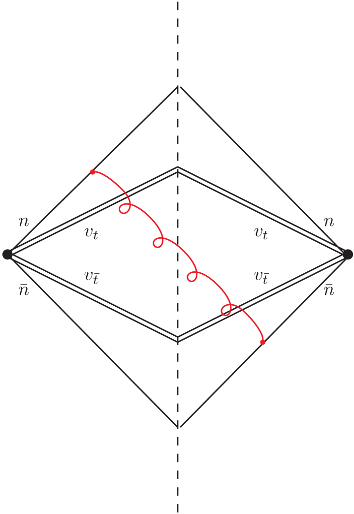
(a) Light-light correlation
H

(b) Light-heavy correlation
H

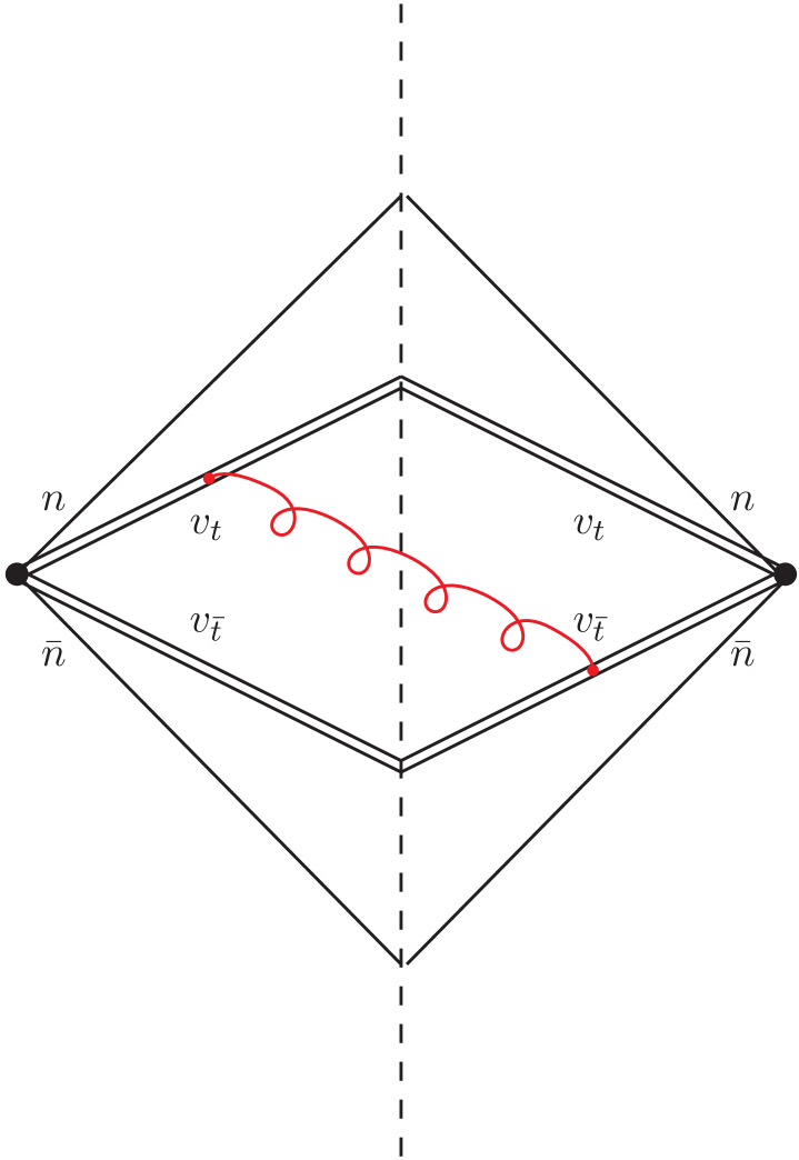
(c) heavy-heavy correlation
H

Figure 4: Representative Feynman diagrams for the NLO soft function. The double line represents the gauge links attached to the top or antitop quark. The single line stands for that from the incoming massless parton, such as gluon, quark, and antiquark.

In the previous parts, we have derived the factorisation formula for the leading singular behaviour of the $q_{\tau}$ spectrum in Eqs. (2.29)-(2.30), which entails the soft functions $\mathcal{S}^{\alpha\beta}_{[\dots]}$ to accommodate the wide angle correlations amongst the active partons. The field-operator definitions of the soft elements have been presented in Eqs. (2.38)-(2.39) in terms of the soft Wilson lines, see [133], sandwiched by the orthonormal colour basis in Eqs. (2.33)-(2.34). In this part, we will calculate the soft function to NLO accuracy. Their three typical contributions are depicted in Fig. 4.

Without any loss of generality, the fixed-order results can be parameterised as

$$\mathcal{S}^{\alpha\beta}_{[\kappa]}(\vec{b}_{\mathrm{T}},\mu,\nu)\equiv\sum_{m=0}^{\infty}\,\left[\frac{\alpha_{s}(\mu)}{4\pi}\right]^{m}\,\mathcal{S}^{\alpha\beta,(m)}_{[\kappa]}(\vec{b}_{\mathrm{T}},\mu,\nu)\,,$$ (2.83)

where $\kappa\in\{g_{n}g_{{\bar{n}}},q^{i}_{n}\bar{q}^{j}_{{\bar{n}}},q^{i}_{{\bar{n}}}\bar{q}^{j}_{n}\}$ as that in Eq. (2.26). The coefficients for the first two orders in $\alpha_{s}$ read

$$\mathcal{S}^{\alpha\beta,(0)}_{[\kappa]}(\vec{b}_{\mathrm{T}},\mu,\nu)\,= \;\delta_{\alpha\beta}\,,$$ (2.84)

$$\mathcal{S}^{\alpha\beta,(1)}_{[\kappa]}(\vec{b}_{\mathrm{T}},\mu,\nu)\,= \;\sum_{a,b}\,\langle c^{\alpha}_{\kappa}|\,\mathbf{T}_{a}\!\cdot\mathbf{T}_{b}\,|c^{\beta}_{\kappa}\rangle\;\mathcal{I}_{ab}(\vec{b}_{\mathrm{T}},\mu,\nu)\,.$$ (2.85)

In absence of any soft interactions, the LO result $\mathcal{S}^{\alpha\beta,(0)}_{[\kappa]}$ is equal to the identity matrix as a consequence of the orthonormality of our colour basis in Eqs. (2.33)-(2.34). For the NLO expression, we employ the colour algebra formalism suggested in [162] to illustrate the outcome. Therein, the flavour subscripts $a,b\in\{q,\bar{q},g,t,\bar{t}\}$ denote the active partons participating in the hard kernel. $\mathbf{T}_{a}$ signifies the colour charge operator for the parton $a$, and $\mathbf{T}_{b}$ likewise. $|c_{\kappa}\rangle$ is the vector representation of $c^{\kappa}_{\{a\}}$ in Eqs. (2.33)-(2.34) in colour space. The coefficient function $\mathcal{I}_{ab}$ contains the contributions from the squared soft amplitudes induced by the Wilson lines in Eqs. (2.38)-(2.39). Its expression in the exponential regularisation scheme [98, 99] is

$$\mathcal{I}_{ab}(\vec{b}_{\mathrm{T}},\mu,\nu)\equiv\,-\frac{\left(\mu^{2}e^{\gamma_{\mathrm{E}}}\pi\right)^{\epsilon}}{\pi}\,\lim_{\delta\to 0}\int{\rm d}k_{n}\,{\rm d}k_{{\bar{n}}}\,{\rm d}^{2-2\epsilon}\;\vec{k}_{\mathrm{T}}\,\delta^{+}(k^{2})\,\frac{v_{a}\cdot v_{b}}{(k\cdot v_{a})(k\cdot v_{b})}\,e^{\mathrm{i}\vec{k}_{\mathrm{T}}\cdot\vec{b}_{\mathrm{T}}-b_{0}E_{k}\delta}\Bigg{|}_{\delta\to\frac{1}{\nu}}\,+\mathcal{Z}_{\mathrm{c}.\mathrm{t}.}^{ab}\,,$$ (2.86)

where $b_{0}=2\exp(-\gamma_{\mathrm{E}})$ with $\gamma_{\mathrm{E}}$ being the Euler constant. $\epsilon$ and $\delta$ are the regulators for the virtuality and rapidity divergences, respectively. $v_{a}$ denotes the four-velocity of parton $a$, for instance $n^{\mu}({\bar{n}}^{\mu})$ for $a=q_{n({\bar{n}})}$ and $v^{\mu}_{t(\bar{t})}=P^{\mu}_{t(\bar{t})}/m_{t}$ for the $a=t({\bar{t}})$. $\mathcal{Z}_{\mathrm{c}.\mathrm{t}.}$ stems from the perturbative expansion of the renormalisation constant $\mathcal{Z}_{[\kappa]}^{s}$ and its complex conjugate in Eqs. (2.38-2.39), defined in the $\overline{\text{MS}}$ scheme throughout this paper.

The result of Eq. (2.86) depends on the partons $a$ and $b$. We will first examine the case of $a$ and $b$ being light flavours, $a,b=l\in\{q,\bar{q},g\}$, depicted in Fig. 4(a). Starting with the case $a=b=l$, the light-like nature of the vectors $n$ and ${\bar{n}}$ trivialises the calculation and we have,

$$\mathcal{I}_{ll}(\vec{b}_{\mathrm{T}},\mu,\nu)=0\,,\qquad\mathcal{Z}_{\mathrm{c}.\mathrm{t}.}^{ll}(\vec{b}_{\mathrm{T}},\mu,\nu,\epsilon)=0\,.$$ (2.87)

However, if the participants consist of different light particles, $a=l\neq b=l^{\prime}$, $\mathcal{I}_{ll^{\prime}}$ does not vanish in general. To calculate its contribution, we follow [98] and first integrate out the longitudinal components $k_{n}$ and $k_{{\bar{n}}}$ in line with the exponential regularisation. Then, we expand the result in $\delta$ and truncate the series to $\mathcal{O}(\delta^{0})$. Finally, we carry out the integral over $\vec{k}_{\mathrm{T}}$ with the aid of the dimensional regulator, giving

$$\mathcal{I}_{ll^{\prime}}(\vec{b}_{\mathrm{T}},\mu,\nu)=L^{2}_{\mathrm{T}}-2\,L_{\mathrm{T}}\,L_{\nu}+\frac{\pi^{2}}{6}\,,\qquad\mathcal{Z}_{\mathrm{c}.\mathrm{t}.}^{ll^{\prime}}(\vec{b}_{\mathrm{T}},\mu,\nu,\epsilon)=\frac{2}{\epsilon^{2}}+\frac{2\,}{\epsilon}L_{\nu}\,,$$ (2.88)

where $L_{\nu}=\ln[\mu^{2}/\nu^{2}]$ and $L_{\mathrm{T}}=\ln[b_{\mathrm{T}}^{2}\mu^{2}/b_{0}^{2}]$. We have compared Eq. (2.88) to the expressions in [98] and find the agreement after synchronising the overall colour factors.

In addition to those correlations between the incoming particles, Eq. (2.86) also involves the contributions from the heavy top quark, $h\in\{t,\bar{t}\}$, see Fig. 4(b). The presence of the massive partons complicates the calculation substantially. Since the denominators at this moment are not homogeneous in $k_{n}$ and $k_{{\bar{n}}}$, performing the integral over those longitudinal components is not straightforward, especially when involving the exponent $E_{k}\delta$. To this end, we resort to the Mellin-Barnes (MB) representation [163, 164] to recast the inhomogeneous propagators in a first step. For $\mathcal{I}_{lh}$, we thus apply the following substitution [80, 165],

$$\frac{1}{(k\cdot v_{h})^{\lambda}}\,\xRightarrow[\text{ }]{\textbf{M.B. }}\,-\frac{1}{\Gamma(\lambda)}\frac{1}{4\pi^{2}} \int^{c_{i}+\mathrm{i}\infty}_{c_{i}-\mathrm{i}\infty}{\rm d}z_{1}\,{\rm d}z_{2}\;\Gamma(-z_{1})\,\Gamma(-z_{2})\,\Gamma(\lambda+z_{1}+z_{2})$$ (2.89)

$$\qquad\times\,\left[\frac{(k\cdot n)(v_{h}\cdot{\bar{n}})}{2}\right]^{z_{1}}\,\left[\frac{(k\cdot{{\bar{n}}})(v_{h}\cdot{n})}{2}\right]^{z_{2}}\,\left(-\vec{k}_{\mathrm{T}}\cdot\vec{v}^{\perp}_{h}\right)^{-\lambda-z_{1}-z_{2}}\,,$$

where the contours (or the values $c_{i}$) are chosen such that the poles from $\Gamma(\lambda+z_{1}+z_{2})$ are to the left of the path, while those of $\Gamma(-z_{1})\Gamma(-z_{2})$ are to the right. Integrating the MB-transformed propagators over $k_{n{({\bar{n}})}}$ and $\vec{k}_{\mathrm{T}}$ now follows the similar pattern to that in deriving Eq. (2.88). Then, to perform the $\delta$-expansion, we first make use of the package MB [166] to determine the contours for $z_{1}$ and $z_{2}$, and then feed the outputs to MBasymptotics [167] for deriving the asymptotic series in $\delta$. The remaining integrals are those over $z_{1}$ and $z_{2}$, for which we utilise MBsums [168] to implement Cauchy’s residue theorem and sum up the ensuing residues from the software Mathematica. The final expression is,

$$\mathcal{I}_{lh}(\vec{b}_{\mathrm{T}},\mu,\nu)\,= \;\frac{L^{2}_{\mathrm{T}}}{2}-L_{\mathrm{T}}\,L_{\nu}+2\,L_{\mathrm{T}}\,\ln\left(v_{l}\cdot v_{h}\right)$$

$$\;{}+2\,\mathrm{arcsinh}^{2}\Big{[}|\vec{v}_{h}^{\perp}|\sin(\varphi_{hb})\Big{]}-(2\pi\mathrm{i})\,\mathrm{arcsinh}\Big{[}|\vec{v}_{h}^{\perp}|\cos(\varphi_{hb})\Big{]}\,$$

$$\;{}+\frac{\pi^{2}}{12}+\mathcal{D}_{lh}(\varphi_{hb})+\mathcal{D}_{lh}(-\varphi_{hb})\,,$$ (2.90)

$$\mathcal{Z}_{\mathrm{c}.\mathrm{t}.}^{lh}(\vec{b}_{\mathrm{T}},\mu,\nu,\epsilon)\,= \;\frac{1}{\epsilon^{2}}+\frac{1}{\epsilon}\Big{[}L_{\nu}-2\ln(v_{l}\cdot v_{h})\Big{]}\,,$$ (2.91)

where $\varphi_{hb}$ denotes the azimuthal opening angle between the vectors $\vec{v}_{h}^{\perp}$ and $\vec{b}_{\mathrm{T}}$. The function $\mathcal{D}_{lh}$ is defined as

$$\mathcal{D}_{lh}(\theta)=\frac{4|\vec{v}_{h}^{\perp}|}{\pi}\,\int_{0}^{\frac{\pi}{2}}{\rm d}{\phi}\,\ln\left[\cot(\phi)\right]\,\Bigg{\{}\frac{\cos(\theta+\phi)}{\sqrt{1+|\vec{v}_{h}^{\perp}|^{2}\sin^{2}(\theta+\phi)}}\arcsin\bigg{[}\frac{|\vec{v}_{h}^{\perp}|\cos(\theta+\phi)}{\sqrt{1+|\vec{v}_{h}^{\perp}|^{2}}}\bigg{]}\Bigg{\}}\,.$$ (2.92)

An analogous strategy is also applicable for the evaluations of the $a=b=h$ and $a=h\neq b=h^{\prime}$ cases, $\mathcal{I}_{hh}$ and $\mathcal{I}_{hh^{\prime}}$, of Fig. 4(c). Since rapidity divergences do not emerge from those time-like gauge links, we can set the regulator $\delta=0$ from the beginning and solve the $k^{\mu}$-integrals in the conventional dimensional regularisation. The results exhibit explicit $z_{1}$ and $z_{2}$ dependences, which are treated with the above MB-Tools [166, 168] to complete the inverse MB transformations. Eventually, they yield,

$$\mathcal{I}_{hh}(\vec{b}_{\mathrm{T}},\mu,\nu)\,= \;2\,L_{\mathrm{T}}\,+\frac{{r}^{h}_{b}}{\sqrt{1+({r}^{h}_{b})^{2}}}\Bigg{[}4\,\mathrm{arcsinh}({r}^{h}_{b})-(2\pi\mathrm{i})\Bigg{]}\,,$$ (2.93)

$$\mathcal{Z}^{hh}_{\mathrm{c.t.}}(\vec{b}_{\mathrm{T}},\mu,\nu,\epsilon)\,= \;-\frac{2}{\epsilon}\,,$$ (2.94)

$$\mathcal{I}_{hh^{\prime}}(\vec{b}_{\mathrm{T}},\mu,\nu)\,= \;L_{\mathrm{T}}\,\frac{4\,v_{h}\cdot v_{h^{\prime}}}{\sqrt{(v_{h}\cdot v_{h^{\prime}})^{2}-1}}\,\mathrm{arctanh}\bigg{[}\sqrt{\frac{v_{h}\cdot v_{h^{\prime}}-1}{v_{h}\cdot v_{h^{\prime}}+1}}\bigg{]}$$

$$\;+\int_{0}^{1}{\rm d}\zeta\,\frac{{r}^{hh^{\prime}}_{b}(\zeta)}{\sqrt{1+\left({r}^{hh^{\prime}}_{b}(\zeta)\right)^{2}}}\,\left(\frac{v_{h}\cdot v_{h^{\prime}}}{{v}^{2}_{hh^{\prime}}(\zeta)}\right)\,\Bigg{[}4\,\mathrm{arcsinh}\left({r}^{hh^{\prime}}_{b}(\zeta)\right)-(2\pi\mathrm{i})\Bigg{]}\,,$$ (2.95)

$$\mathcal{Z}^{hh^{\prime}}_{\mathrm{c.t.}}(\vec{b}_{\mathrm{T}},\mu,\nu,\epsilon)\,= \;-\frac{1}{\epsilon}\frac{4\,v_{h}\cdot v_{h^{\prime}}}{\sqrt{(v_{h}\cdot v_{h^{\prime}})^{2}-1}}\,\mathrm{arctanh}\bigg{[}\sqrt{\frac{v_{h}\cdot v_{h^{\prime}}-1}{v_{h}\cdot v_{h^{\prime}}+1}}\bigg{]}\,,$$ (2.96)

where

$${v}^{\mu}_{hh^{\prime}}(\zeta)\,=\;\zeta\,v_{h}^{\mu}+(1-\zeta)\,v_{h^{\prime}}^{\mu}\,,\qquad{r}^{h}_{b}\,=\;\widehat{b}_{\mathrm{T}}\cdot\vec{v}^{\perp}_{h}\,,\qquad{r}^{hh^{\prime}}_{b}(\zeta)\,=\;\widehat{b}_{\mathrm{T}}\cdot\frac{\vec{v}_{hh^{\prime}}^{\perp}(\zeta)}{\sqrt{v^{2}_{hh^{\prime}}(\zeta)}}\,.$$ (2.97)

During the calculations, we have exploited the on-shell conditions $v_{t}^{2}=v_{\bar{t}}^{2}=1$ and introduced the definition $\widehat{b}_{\mathrm{T}}\equiv\vec{b}_{\mathrm{T}}/b_{\mathrm{T}}$.

With all relevant coefficient functions $\mathcal{I}_{ab}$ at hand, together with the colour factors of Eq. (2.85), we can now establish the NLO soft function together with the renormalisation constants $\mathcal{Z}^{s}_{[\kappa]}$. For the latter case, we have checked that the results in Eqs. (2.88)-(2.96) indeed satisfy the identity in Eq. (2.80), where the hard and beam renormalisation constants are extracted from [134] and [141, 142], respectively. Regarding the renormalised finite parts $\mathcal{I}_{ab}$, we compare our expressions with those from the CSS framework [66] at the scale $\mu=\nu=b_{0}^{2}/b_{\mathrm{T}}^{2}$ and find full agreement. Furthermore, since during the derivation we did not utilise the relationship $\vec{v}_{t}^{\perp}+\vec{v}_{\bar{t}}^{\perp}=\vec{0}$ for simplification, the results in Eqs. (2.88-2.5) are also comparable with the soft function in the process $pp\to{t{\bar{t}}}H$ [148]. However, at this moment, although the real parts of $\mathcal{I}_{ab}$ still coincide with those in [148], the signs in front of the terms $2\pi\mathrm{i}$ in Eq. (2.5), Eq. (2.93), and Eq. (2.5) are inverted. This purely imaginary term does not enter the present calculation on the ${t{\bar{t}}}$ production or the comparison with [66], as these imaginary contributions cancel through the momentum conservation $\vec{v}_{t}^{\perp}+\vec{v}_{\bar{t}}^{\perp}=\vec{0}$. Nonetheless, this difference can influence the transverse momentum spectrum in ${t{\bar{t}}}H$ production, or similar processes, especially within the domain $M_{{t{\bar{t}}}H}\gtrsim M_{t{\bar{t}}}\sim 2m_{t}$. We leave it to a forthcoming publication to elaborate on those processes and, in particular, deliver a numeric comparison of our results, to those from [148], and a fixed-order QCD calculation from S HERPA  [169, 170, 171].

3 Resummation

In the previous section we have analysed the dynamic regions contributing to the leading singularities in Eq. (2.6) and established the corresponding factorisation formula in impact parameter space. This section will now be devoted to the resummation of these asymptotic behaviours.

3.1 Asymptotic behavior

We start with identifying the singular terms in Eq. (2.43). Therefore, without loss of generality, we parametrise the perturbative expansion of $\widetilde{\Sigma}_{{t{\bar{t}}}}$ as follows,

$$\widetilde{\Sigma}_{{t{\bar{t}}}}\,\sim\,\sum_{m,n}\,\alpha^{m}_{s}(M_{t{\bar{t}}})\;L^{n}_{\mathrm{M}}\,\Big{\{}s_{m,n}(\beta_{t{\bar{t}}},x_{t},Y_{t{\bar{t}}})+a_{m,n}(\mathrm{sign}[b_{\tau_{\|}}],\beta_{t{\bar{t}}},x_{t},Y_{t{\bar{t}}})\Big{\}}\;,$$ (3.1)

where $L_{\mathrm{M}}\equiv\log\left[{{b}^{2}_{\tau_{\|}}M_{t{\bar{t}}}^{2}}/{b_{0}^{2}}\right]$ collects all the relevant dimensionful quantities. Order by order, there are two dimensionless coefficients, $s_{m,n}$ and $a_{m,n}$. While both depend on $\beta_{t{\bar{t}}}$, $x_{t}$, and $Y_{t{\bar{t}}}$, $s_{m,n}$ is independent of the magnitude and orientation of the impact parameter. Thus, we will refer them to the azimuthal symmetric terms (AST) hereafter. On the other hand, in presence of the helicity-flipping beam radiation in Eq. (2.36) and the wide angle soft correlations from Eqs. (2.38)-(2.39), $\widetilde{\Sigma}_{{t{\bar{t}}}}$ also contains contributions sensitive to the orientation of the impact parameter, i.e. the azimuthal asymmetric term (AAT) $a_{m,n}$ [73, 67]. Since the rejection component $b_{\tau_{\perp}}$ has been integrated out in Eq. (2.42), the orientation dependence is reduced to a dependence on the sign of $b_{\tau_{\|}}$ in Eq. (3.1). Please note, in deriving eq. (3.1), we have set the scales $\mu=\nu=M_{t{\bar{t}}}$ in Eqs. (2.29)-(2.30) and then extracted the $L_{\mathrm{M}}$ terms through dimensional analysis. Other scales choices $\{\mu,\nu\}$ lead to the same result after regrouping the dimensional quantities appropriately, on account of the (rapidity) renormalisation group discussed in Sec. 2.4.3.

From Eq. (3.1), we can evaluate the $q_{\tau}$ spectrum by completing the inverse Fourier transformation in Eq. (2.43). Exploiting the fact that the function $\cos(b_{\tau_{\|}}q_{\tau})$ is even under the integral over $b_{\tau_{\|}}$, we have

$$\frac{{\rm d}{\sigma_{{t{\bar{t}}}}}}{{\rm d}M_{t{\bar{t}}}^{2}\,{\rm d}^{2}\vec{P}_{t}^{\perp}\,{\rm d}Y_{t{\bar{t}}}\,{\rm d}q_{\tau}}\,\sim \;\sum\limits_{m,n}\int^{\infty}_{-\infty}{\rm d}b_{\tau_{\|}}\,\cos(b_{\tau_{\|}}q_{\tau})\,L^{n}_{\mathrm{M}}\,\Big{\{}s_{m,n}(\beta_{t{\bar{t}}},x_{t},Y_{t{\bar{t}}})+a_{m,n}(\mathrm{sign}[b_{\tau_{\|}}],\beta_{t{\bar{t}}},x_{t},Y_{t{\bar{t}}})\Big{\}}$$ (3.2)

$$\,= \;\sum\limits_{m,n}\Big{\{}2s_{m,n}(\beta_{t{\bar{t}}},x_{t},Y_{t{\bar{t}}})+a_{m,n}^{+}(\beta_{t{\bar{t}}},x_{t},Y_{t{\bar{t}}})+a_{m,n}^{-}(\beta_{t{\bar{t}}},x_{t},Y_{t{\bar{t}}})\Big{\}}\;\mathcal{F}^{(n)}_{\tau}(q_{\tau},M_{t{\bar{t}}})\,,$$

where $a_{m,n}^{\pm}$ are the decomposition of the AAT components according to $\mathrm{sign}[b_{\tau_{\|}}]$ and the function $\mathcal{F}^{(n)}_{\tau}$ is defined as,

$$\mathcal{F}^{(n)}_{\tau}(q_{\tau},M_{t{\bar{t}}})=\int^{\infty}_{0}{\rm d}b_{\tau_{\|}}\,\cos(b_{\tau_{\|}}q_{\tau})\,L^{n}_{\mathrm{M}}\,.$$ (3.3)

To appraise $\mathcal{F}^{(n)}_{\tau}(q_{\tau},M_{t{\bar{t}}})$, we follow the strategy of [102] and introduce the generating function,

$$\mathbf{F}_{\tau}(\eta,q_{\tau},M_{t{\bar{t}}})\,= \;\sum_{n=0}^{\infty}\,\frac{\eta^{n}}{n!}\,\mathcal{F}^{(n)}_{\tau}(q_{\tau},M_{t{\bar{t}}})\,=\;\int^{\infty}_{0}{\rm d}{b}_{\tau_{\|}}\,\cos\left({b}_{\tau_{\|}}{q}_{\tau}\right)\,\left(\frac{{b}^{2}_{\tau_{\|}}M_{t{\bar{t}}}^{2}}{b_{0}^{2}}\right)^{\eta}$$

$$= \;-\frac{4^{-\eta}e^{2\gamma_{\mathrm{E}}\eta}\,\sin(\pi\eta)\,\Gamma[2\eta+1]}{{q}_{\tau}}\,\left(\frac{M_{t{\bar{t}}}^{2}}{q^{2}_{\tau}}\right)^{\eta}\,.$$ (3.4)

Hence, $\mathcal{F}^{(n)}_{\tau}(q_{\tau},M_{t{\bar{t}}})$ corresponds to the $n$-th derivative of $\mathbf{F}_{\tau}(\eta,q_{\tau},M_{t{\bar{t}}})$ with respect to $\eta$ at the point $\eta=0$. The results of the first few ranks read

$$\begin{split}\mathcal{F}^{(0)}_{\tau}(q_{\tau},M_{t{\bar{t}}})\,=&\;\;0\,,\\ \mathcal{F}^{(1)}_{\tau}(q_{\tau},M_{t{\bar{t}}})\,=&\;-\frac{\pi}{q_{\tau}}\,,\\ \mathcal{F}^{(2)}_{\tau}(q_{\tau},M_{t{\bar{t}}})\,=&\;-\frac{2\pi}{q_{\tau}}\ln\left[\frac{M_{t{\bar{t}}}^{2}}{4q_{\tau}^{2}}\right]\,,\\ \mathcal{F}^{(3)}_{\tau}(q_{\tau},M_{t{\bar{t}}})\,=&\;-\frac{3\pi}{q_{\tau}}\ln^{2}\left[\frac{M_{t{\bar{t}}}^{2}}{4q_{\tau}^{2}}\right]\,-\frac{\pi^{3}}{q_{\tau}},\\ \mathcal{F}^{(4)}_{\tau}(q_{\tau},M_{t{\bar{t}}})\,=&\;-\frac{4\pi}{q_{\tau}}\ln^{3}\left[\frac{M_{t{\bar{t}}}^{2}}{4q_{\tau}^{2}}\right]\,-\frac{4\pi^{3}}{q_{\tau}}\ln\left[\frac{M_{t{\bar{t}}}^{2}}{4q_{\tau}^{2}}\right]\,+\frac{64\pi\zeta_{3}}{q_{\tau}},\\ \vdots\;&\\ \mathcal{F}^{(k)}_{\tau}(q_{\tau},M_{t{\bar{t}}})\,=&\;-\frac{k\pi}{q_{\tau}}\ln^{k-1}\left[\frac{M_{t{\bar{t}}}^{2}}{4q_{\tau}^{2}}\right]+\ldots\,.\end{split}$$ (3.5)

Here we have focussed on the regime where $q_{\tau}$ is small, but always larger than 0. Otherwise, contributions such as $\delta[q_{\tau}]$ will enter the expressions above. From these results, it is observed that the coefficients $s_{m,n}$ and $a_{m,n}^{\pm}$ cannot induce any divergent behaviour by themselves as exhibited in Eq. (3.5), whilst the logarithmic terms $L_{\mathrm{M}}^{k}$ produce the singular series up to $\ln^{k-1}[{M_{t{\bar{t}}}^{2}}/{(4q_{\tau}^{2})}]/q_{\tau}$, i.e.  the entire LP asymptotic behaviors of Eq. (2.6). As a consequence, the resummation of the $q_{\tau}$ spectrum can now be expressed as an exponentiation of the $L_{\mathrm{M}}$, resembling the corresponding resummation in the Drell-Yan processes and Higgs production [100, 101, 102, 103, 107, 108, 109, 96, 97, 98, 99]. In Sec. 3.2, we will use the solutions of RaGE and RGE to accomplish this exponentiation.

It is interesting to note that, by analogy to the $q_{\tau}$ resummation, the leading singular behaviour of the azimuthally averaged $q_{\mathrm{T}}$ distribution is also governed by the characteristic logarithmic terms from the impact space [64, 65], such that the R(a)GE framework is in principle applicable therein as well to accomplish the resummation. However, aside from those two observables, the transverse momentum resummation is generally more involved on the $pp\to{t{\bar{t}}}+X$ process. For instance, the singular behaviour of the double differential observable ${\rm d}\sigma_{{t{\bar{t}}}}/{\rm d}\vec{q}_{\mathrm{T}}$ is not only contained in the logarithmic terms, but the AATs can also make up in part the asymptotic series [67]. The appearance of these asymmetric divergent terms can have non-trivial impacts on the pattern of the LP singularities and the choice of resummation scheme. In App. A, we will deliver a comparative study on this issue.

3.2 Evolution equations

We will now elaborate on the evolution equations of the hard, beam, and soft functions introduced in Eqs. (2.29)-(2.30).

The hard function, see Eqs. (2.31)-(2.32), contains the squared UV-renormalised amplitudes multiplied by the IRC regulator. Considering that the scale dependences induced by the UV renormaliation cancel fully within the amplitudes, the evolution equation of the hard sector is governed solely by the IRC counterterm $\mathcal{Z}^{h}_{[\kappa]}$. According to the parametrisation of [134, 172, 51], we have,

$$\frac{{\rm d}}{{\rm d}\ln\mu^{2}}\,\mathcal{H}^{[\kappa]}_{\alpha\beta}\big{(}M_{t{\bar{t}}}^{2},\beta_{t{\bar{t}}},x_{t},\mu\big{)}\,= \;-C_{[\kappa]}\,\Gamma_{\mathrm{cusp}}\,\ln\left[\frac{\mu^{2}}{M_{t{\bar{t}}}^{2}}\right]\,\mathcal{H}^{[\kappa]}_{\alpha\beta}\big{(}M_{t{\bar{t}}}^{2},\beta_{t{\bar{t}}},x_{t},\mu\big{)}\,$$

$$\;{}+\sum_{\gamma}\left[\frac{\mathbf{\gamma}^{[\kappa]}_{h,\beta\gamma}}{2}\,\mathcal{H}^{[\kappa]}_{\alpha\gamma}\big{(}M_{t{\bar{t}}}^{2},\beta_{t{\bar{t}}},x_{t},\mu\big{)}+\left(\frac{\mathbf{\gamma}^{[\kappa]}_{h,\alpha\gamma}}{2}\right)^{\!\!\!*}\mathcal{H}^{[\kappa]}_{\gamma\beta}\big{(}M_{t{\bar{t}}}^{2},\beta_{t{\bar{t}}},x_{t},\mu\big{)}\right]\,,$$ (3.6)

where the subscripts $\{\alpha,\beta,\gamma\}$ represent the colour indices in the set of colour basis in Eqs. (2.33)-(2.34). The helicity indices involved in the gluonic channel have been omitted for brevity. $\kappa$ runs over $\{g_{n}g_{{\bar{n}}},q^{i}_{n}\bar{q}^{j}_{{\bar{n}}},q^{i}_{{\bar{n}}}\bar{q}^{j}_{n}\}$, indicating the partonic channel. $C_{[\kappa]}$ denotes the colour factor in QCD with

$$\kappa\in\{g_{n}g_{{\bar{n}}}\}\,:\;C_{[\kappa]}=C_{A}\;,\qquad\qquad\kappa\in\{q^{i}_{n}\bar{q}^{j}_{{\bar{n}}},q^{i}_{{\bar{n}}}\bar{q}^{j}_{n}\}\,:\;C_{[\kappa]}=C_{F}\,.$$ (3.7)

$\Gamma_{\mathrm{cusp}}$ is the cusp anomalous dimension. It is needed to three-loop accuracy [173] in this paper, but is available to four-loop precision in the literature [174, 175]. A numeric estimation of the five-loop contribution is addressed in [176]. Analogously, $\gamma^{[\kappa]}_{h}$ is the non-cusp anomalous dimension for the hard contribution. Their analytic expressions up to N²LO can be found in [134, 172] and progress towards the three-loop result has been made in [177].

The quark and gluon beam functions are given in Eqs. (2.35)-(2.36) in terms of the SCET_II field operators. They are same as those participating into the Drell-Yan processes and Higgs production. They admit the RGEs [98],

$$\frac{\partial}{\partial\ln\mu^{2}}\ln\mathcal{B}_{n}^{[q_{n}^{i}]}(\eta_{n},b_{\mathrm{T}},\mu,\nu)\,= \;C_{F}\,\Gamma_{\mathrm{cusp}}\,\ln\bigg{[}\frac{\nu}{\eta_{n}\,\sqrt{s}}\bigg{]}+\gamma^{[q]}_{b}\;,$$ (3.8)

$$\frac{\partial}{\partial\ln\mu^{2}}\ln\mathcal{B}^{[g_{n}]}_{n,h^{\prime}h}(\eta_{n},\vec{b}_{\mathrm{T}},\mu,\nu)\,= \;C_{A}\,\Gamma_{\mathrm{cusp}}\,\ln\bigg{[}\frac{\nu}{\eta_{n}\,\sqrt{s}}\bigg{]}+\gamma^{[g]}_{b}\;,$$ (3.9)

as well as the RaGEs [98],

$$-\frac{2}{C_{F}}\,\frac{\partial}{\partial\ln\nu^{2}}\ln\mathcal{B}_{n}^{[q_{i}]}(\eta_{n},b_{\mathrm{T}},\mu,\nu)\,= \;-\frac{2}{C_{A}}\,\frac{\partial}{\partial\ln\nu^{2}}\ln\mathcal{B}^{[g_{n}]}_{n,h^{\prime}h}(\eta_{n},\vec{b}_{\mathrm{T}},\mu,\nu)$$

$$\,= \;\gamma_{r}\left[\alpha_{s}\left(\frac{b_{0}}{b_{\mathrm{T}}}\right)\right]\,+\int_{\mu^{2}}^{\frac{b_{0}^{2}}{b_{\mathrm{T}}^{2}}}\,\frac{{\rm d}\bar{\mu}^{2}}{\bar{\mu}^{2}}\,\Gamma_{\mathrm{cusp}}\left[\alpha_{s}(\bar{\mu})\right]\,.$$ (3.10)

Here, $\eta_{n}$ stands for the momentum fraction along the $n$ direction. $\gamma^{[q,g]}_{b}$ and $\gamma_{r}$ are the non-cusp anomalous dimensions brought about in the virtuality and rapidity renormalisations, respectively. Their specific expressions are dependent on the choice of regularisation prescription, and this work will use those that correspond with our choice of using the exponential rapidity regulator [98]. They are known at N²LO accuracy [142, 141], which we use in the following. N³LO results are also available in the literature [99, 178, 143, 179, 144], and N⁴LO corrections [180, 181, 182, 183] have appeared recently.

In order to derive the evolution equations for the soft sector, we utilise the scale invariance condition in Eq. (2.81) and the R(a)GEs above. It follows that

$$\frac{\partial}{\partial\ln\mu^{2}}\mathcal{S}_{[\kappa]}^{\alpha\beta}\big{(}\vec{b}_{\mathrm{T}},\mu,\nu\big{)}\,= \;-\bigg{\{}C_{[\kappa]}\,\Gamma_{\mathrm{cusp}}\,\ln\left[\frac{\nu^{2}}{\mu^{2}}\right]+2\gamma_{b}^{[\kappa]}\bigg{\}}\,\mathcal{S}_{[\kappa]}^{\alpha\beta}\big{(}\vec{b}_{\mathrm{T}},\mu,\nu\big{)}$$

$$\;-\sum_{\gamma}\,\left[\mathcal{S}_{[\kappa]}^{\alpha\gamma}\big{(}\vec{b}_{\mathrm{T}},\mu,\nu\big{)}\,\frac{\mathbf{\gamma}^{[\kappa]}_{h,\gamma\beta}}{2}+\mathcal{S}_{[\kappa]}^{\gamma\beta}\big{(}\vec{b}_{\mathrm{T}},\mu,\nu\big{)}\,\left(\frac{\mathbf{\gamma}^{[\kappa]}_{h,\gamma\alpha}}{2}\right)^{\!\!\!*}\,\right]\,,$$ (3.11)

and

$$\frac{1}{C_{[\kappa]}}\,\frac{\partial}{\partial\ln\nu^{2}}\ln\mathcal{S}^{\alpha\beta}_{[\kappa]}\big{(}\vec{b}_{\mathrm{T}},\mu,\nu\big{)}\,= \;\gamma_{r}\left[\alpha_{s}\left(\frac{b_{0}}{b_{\mathrm{T}}}\right)\right]\,+\int_{\mu^{2}}^{\frac{b_{0}^{2}}{b_{\mathrm{T}}^{2}}}\,\frac{{\rm d}\bar{\mu}^{2}}{\bar{\mu}^{2}}\,\Gamma_{\mathrm{cusp}}\left[\alpha_{s}(\bar{\mu})\right]\,.$$ (3.12)

For brevity, we make use of $\gamma_{b}^{[\kappa]}$ here to represent the virtuality anomalous dimensions in Eqs. (3.8)-(3.9), more specifically,

$$\kappa\in\{g_{n}g_{{\bar{n}}}\}\,:\;\gamma_{b}^{[\kappa]}=\gamma_{b}^{[g]}\,,\qquad\qquad\kappa\in\{q^{i}_{n}\bar{q}^{j}_{{\bar{n}}},q^{i}_{{\bar{n}}}\bar{q}^{j}_{n}\}\,:\;\gamma_{b}^{[\kappa]}=\gamma_{b}^{[q]}\,.$$ (3.13)

As observed in Eqs. (3.11)-(3.12), since the anomalous dimensions herein are all independently extracted from the hard and beam functions, these evolution equations provide a non-trivial opportunity to examine our soft function of Sec. 2.5 and in turn the factorisation in Eqs. (2.29)-(2.30). Substituting the expressions of Eq. (2.85) into Eqs. (3.11)-(3.12), we have checked that our results indeed satisfy the criteria above on the scale dependences.

Solving those RGEs and RaGEs permits us to bridge the intrinsic scales of the hard, beam, and soft ingredients, thereby exponentiating the characteristic logarithmic terms in Eq. (3.1). Substituting these solutions into the master formula of Eq. (2.43), we arrive at the resummed $q_{\tau}$ spectrum,

$$\frac{{\rm d}{\sigma^{\mathrm{res}}_{{t{\bar{t}}}}}}{{\rm d}M_{t{\bar{t}}}^{2}\,{\rm d}^{2}\vec{P}_{t}^{\perp}\,{\rm d}Y_{t{\bar{t}}}\,{\rm d}q_{\tau}}\,= \;\sum_{\mathrm{sign}[x_{t}]}\frac{\Theta_{\mathrm{kin}}^{(0)}}{16\pi^{3}\,\beta_{t{\bar{t}}}\,|x_{t}|\,M^{4}_{{t{\bar{t}}}}\,s}\sum_{\kappa}\int^{\infty}_{-\infty}{\rm d}{b}_{\tau_{\|}}\,\cos\left({b}_{\tau_{\|}}{q}_{\tau}\right)\,\widetilde{\Sigma}_{{t{\bar{t}}}}^{\mathrm{res},[\kappa]}(b_{\tau_{\|}}\vec{\tau},M_{t{\bar{t}}},\beta_{t{\bar{t}}},x_{t},Y_{t{\bar{t}}})\,,$$ (3.14)

where

$$\widetilde{\Sigma}_{{t{\bar{t}}}}^{\mathrm{res},[q^{i}_{n}\bar{q}^{j}_{{\bar{n}}}]}(\vec{b}_{\mathrm{T}},M_{t{\bar{t}}},\beta_{t{\bar{t}}},x_{t},Y_{t{\bar{t}}})$$ (3.15)

$$\,= \;\left(\frac{1}{2N_{c}}\right)^{2}\,\mathcal{D}^{\mathrm{res}}_{[q^{i}_{n}\bar{q}^{j}_{{\bar{n}}}]}(b_{\mathrm{T}},M_{t{\bar{t}}},\mu_{h},\mu_{b},\mu_{s},\nu_{b},\nu_{s})\,\times\mathcal{B}_{n}^{[q_{n}^{i}]}(\eta_{n},b_{\mathrm{T}},\mu_{b},\nu_{b})\,\mathcal{B}_{{\bar{n}}}^{[\bar{q}_{\bar{n}}^{j}]}(\eta_{{\bar{n}}},b_{\mathrm{T}},\mu_{b},\nu_{b})\,$$

$$\sum_{\{\alpha,\beta\}}\Bigg{\{}\mathcal{S}^{\alpha_{1}\beta_{1}}_{[q_{n}\bar{q}_{{\bar{n}}}]}(\vec{b}_{\mathrm{T}},\mu_{s},\nu_{s})\left[\mathcal{V}^{[q_{n}\bar{q}_{{\bar{n}}}]}_{\alpha_{1}\alpha_{2}}(\beta_{t{\bar{t}}},x_{t},\mu_{s},\mu_{h})\right]^{*}\,\mathcal{V}^{[q_{n}\bar{q}_{{\bar{n}}}]}_{\beta_{1}\beta_{2}}(\beta_{t{\bar{t}}},x_{t},\mu_{s},\mu_{h})\,\mathcal{H}_{\alpha_{2}\beta_{2}}^{[q^{i}_{n}\bar{q}^{j}_{{\bar{n}}}]}(M_{t{\bar{t}}},\beta_{t{\bar{t}}},x_{t},\mu_{h})\,\Bigg{\}}\,,$$

$$\widetilde{\Sigma}_{{t{\bar{t}}}}^{\mathrm{res},[g_{n}g_{{\bar{n}}}]}(\vec{b}_{\mathrm{T}},M_{t{\bar{t}}},\beta_{t{\bar{t}}},x_{t},Y_{t{\bar{t}}})$$ (3.16)

$$\,= \;\left(\frac{1}{N^{2}_{c}-1}\right)^{2}\,\mathcal{D}^{\mathrm{res}}_{[g_{n}g_{{\bar{n}}}]}(b_{\mathrm{T}},M_{t{\bar{t}}},\mu_{h},\mu_{b},\mu_{s},\nu_{b},\nu_{s})\,\sum_{\{\alpha,\beta,h,h^{\prime}\}}\Bigg{\{}\mathcal{S}^{\alpha_{1}\beta_{1}}_{[g_{n}g_{{\bar{n}}}]}(\vec{b}_{\mathrm{T}},\mu_{s},\nu_{s})\,$$

$$\times\,\mathcal{B}^{[g_{n}]}_{n,h_{n}^{\prime}{h_{n}}}(\eta_{n},\vec{b}_{\mathrm{T}},\mu_{b},\nu_{b})\,\mathcal{B}^{[g_{{\bar{n}}}]}_{{\bar{n}},h_{{\bar{n}}}^{\prime}{h_{{\bar{n}}}}}(\eta_{{\bar{n}}},\vec{b}_{\mathrm{T}},\mu_{b},\nu_{b})\,\left[\mathcal{V}^{[g_{n}g_{{\bar{n}}}]}_{\alpha_{1}\alpha_{2}}(\beta_{t{\bar{t}}},x_{t},\mu_{s},\mu_{h})\right]^{*}\,\mathcal{V}^{[g_{n}g_{{\bar{n}}}]}_{\beta_{1}\beta_{2}}(\beta_{t{\bar{t}}},x_{t},\mu_{s},\mu_{h})\,$$

$$\times\mathcal{H}_{\alpha_{2}\beta_{2};{h_{{\bar{n}}}^{\prime}}h_{{\bar{n}}};{h_{n}^{\prime}}h_{n}}^{[g_{n}g_{{\bar{n}}}]}(M_{t{\bar{t}}},\beta_{t{\bar{t}}},x_{t},\mu_{h})\,\Bigg{\}}\,.$$

The expression of $\widetilde{\Sigma}_{{t{\bar{t}}}}^{\mathrm{res},[q^{i}_{{\bar{n}}}\bar{q}^{j}_{n}]}$ can be obtained from Eq. (3.15) by adjusting the label momenta of the beam-collinear modes as appropriate. As is apparent in Eqs. (3.15-3.16), two sets of auxiliary scales $\{\mu_{h},\mu_{b},\mu_{s}\}$ and $\{\nu_{b},\nu_{s}\}$ have been introduced to define the initial conditions utilised in solving the RaGEs and RGEs above. An appropriate choice of their values minimises the missing higher-order corrections, and in this paper, in a bid to minimise the logarithmic dependences on the respective sectors, the following values will be taken as defaults in this paper [97, 184],

$$\mu^{\mathrm{def}}_{h}=\nu^{\mathrm{def}}_{b}=M_{t{\bar{t}}}\,,\quad\mu^{\mathrm{def}}_{b}=\mu^{\mathrm{def}}_{s}=\nu^{\mathrm{def}}_{s}=b_{0}/|b_{\tau_{\|}}|\,.$$ (3.17)

With the choices in Eq. (3.17), the impact space integral in Eq. (3.14) may approach or cross the Landau singularity in the large $|b_{\tau_{\|}}|$ regime. In order to avoid the divergence, we impose upper and lower boundaries $|b_{\tau_{\|}}|\leq b^{\mathrm{cut}}_{\tau_{\|}}=2\,\text{GeV}^{-1}$ in Eq. (3.14) [184]. Alternative schemes have been discussed in [107, 185].

Further, Eqs. (3.15)-(3.16) also include the kernels $\mathcal{D}^{\mathrm{res}}_{[\kappa]}$ and $\mathcal{V}^{[\kappa]}_{\alpha\beta}$ to evolve the intrinsic scales amongst the fixed-order functions. $\mathcal{D}^{\mathrm{res}}_{[\kappa]}$ is induced by the diagonal anomalous dimensions, such as $\gamma_{\mathrm{cusp}}$, $\gamma_{b}^{[\kappa]}$, and $\gamma_{r}$ in Eqs. (3.2)-(3.10). Its definition reads

$$\ln\mathcal{D}^{\mathrm{res}}_{[\kappa]}(b_{\mathrm{T}},M_{t{\bar{t}}},\mu_{h},\mu_{b},\mu_{s},\nu_{b},\nu_{s})$$

$$\,=\;\int^{\mu^{2}_{s}}_{\mu^{2}_{b}}\,\frac{{\rm d}\bar{\mu}^{2}}{\bar{\mu}^{2}}\,\Bigg{\{}C_{[\kappa]}\,\Gamma_{\mathrm{cusp}}\big{[}\alpha_{s}(\bar{\mu})\big{]}\,\ln\bigg{[}\frac{\nu_{b}^{2}}{M_{t{\bar{t}}}^{2}}\bigg{]}+2\,\gamma^{[\kappa]}_{b}\big{[}\alpha_{s}(\bar{\mu})\big{]}\,\Bigg{\}}-\int^{\mu_{s}^{2}}_{\mu_{h}^{2}}\frac{{\rm d}\bar{\mu}^{2}}{\bar{\mu}^{2}}\,\bigg{\{}{C_{[\kappa]}}\,\Gamma_{\mathrm{cusp}}\big{[}\alpha_{s}(\bar{\mu})\big{]}\,\ln\left[\frac{\bar{\mu}^{2}}{M_{t{\bar{t}}}^{2}}\right]\,\bigg{\}}$$

$$\,\phantom{=}\;{}+C_{[\kappa]}\,\ln\bigg{[}\frac{\nu_{s}^{2}}{\nu_{b}^{2}}\bigg{]}\,\int_{\frac{b_{0}^{2}}{b_{\mathrm{T}}^{2}}}^{\mu_{s}^{2}}\,\frac{{\rm d}\bar{\mu}^{2}}{\bar{\mu}^{2}}\,\Gamma_{\mathrm{cusp}}\big{[}\alpha_{s}(\bar{\mu})\big{]}\,-C_{[\kappa]}\,\ln\bigg{[}\frac{\nu_{s}^{2}}{\nu_{b}^{2}}\bigg{]}\,\gamma_{r}\bigg{[}\alpha_{s}\left(\frac{b_{0}}{b_{\mathrm{T}}}\right)\bigg{]}\,.$$ (3.18)

$\mathcal{V}^{[\kappa]}_{\alpha\beta}$ accounts for the contributions from the non-diagonal anomalous dimension $\gamma_{h,\alpha\beta}^{[\kappa]}$, which, in principle, can be extracted from the solutions of the RGE of the hard function in Eq. (3.2). However, in the presence of the non-diagonal elements in $\gamma_{h}^{[\kappa]}$, it is somewhat challenging to achieve a closed expression. Hence, in this work we adopt the perturbative approaches suggested in [186, 187, 51]. The details on the implementation are collected in App. B.

Logarithmic accuracy$\int_{A}^{B}$	$\mathcal{H}$, $\mathcal{S}$, $\mathcal{B}$	$\Gamma_{\text{cusp}}$	$\gamma_{h,s,b,r}$
NLL′ $\int_{A}^{B}$	$\mathcal{O}(\alpha^{0}_{s})$	$\mathcal{O}(\alpha^{2}_{s})$	$\mathcal{O}(\alpha_{s})$
N2LL $\int_{A}^{B}$	$\mathcal{O}(\alpha_{s})$	$\mathcal{O}(\alpha^{3}_{s})$	$\mathcal{O}(\alpha^{2}_{s})$
N2LL′ $\int_{A}^{B}$	$\mathcal{O}(\alpha^{2}_{s})$	$\mathcal{O}(\alpha^{3}_{s})$	$\mathcal{O}(\alpha^{2}_{s})$

Table 1: Precision prerequisites on the anomalous dimensions and the fixed-order functions for a given logarithmic accuracy.

Equipped with Eqs. (3.15)-(3.16), we can calculate the resummed projected transverse momentum distributions. In this work, we will present the results in particular at NLL^′, N²LL, and approximate N²LL^′ levels. For NLL^′, N²LL, and strict N²LL^′ accurate calculations, the required precisions for the various anomalous dimensions and fixed-order functions have been summarised in Table. 1. In particular, for the N²LL^′ result, the hard and soft sectors need to be known at full N²LO accuracy. However, only the logarithmic terms, which are derived from Eq. (3.2) and Eqs. (3.11)-(3.12), are included in this work. We thus label our results with this approximation as aN²LL^′ in the rest of this paper.

3.3 Observables

In Eq. (3.14), we have presented the master formula of the resummed $q_{\tau}$ spectrum with a general choice of $\vec{\tau}$. In Sec. 4, we will investigate three observables, $q_{\mathrm{T,out}}$, $q_{\mathrm{T,in}}$, and $\Delta\Phi_{{t{\bar{t}}}}$. The calculations of the first two observables are immediate from Eq. (3.14) by choosing the reference vector $\vec{\tau}$ to be perpendicular or parallel with respect to the top-quark transverse momentum $\vec{P}_{t}^{\perp}$,

$$q_{\tau}\,=\,~{} q_{\mathrm{T,out}}\,,\qquad\mathrm{if}~{}\vec{\tau}=\pm\;\vec{n}\times\frac{\vec{P}_{t}^{\perp}}{|\vec{P}_{t}^{\perp}|}\,,$$ (3.19)

$$q_{\tau}\,=\,~{} q_{\mathrm{T,in}}\,,\qquad~{}~{}\!\mathrm{if}~{}\vec{\tau}=\pm\;\frac{\vec{P}_{t}^{\perp}}{|\vec{P}_{t}^{\perp}|}\,,$$ (3.20)

where the unit vector $\vec{n}$ characterises the flight direction of one of the colliding protons. Since the value of $q_{\tau}$ only concerns the magnitude of the projected component, the calculation with either $+$ or $-$ sign in Eqs. (3.19)-(3.20) gives the same result. In order to determine the azimuthal distribution $\Delta\Phi_{{t{\bar{t}}}}$, it is worth noting that in the vicinity of $\Delta\Phi_{{t{\bar{t}}}}\to\pi$, we are able to perform the expansion in $\Delta\phi_{{t{\bar{t}}}}\equiv(\pi-\Delta\Phi_{{t{\bar{t}}}})\sim\lambda_{\tau}$,

$$\Delta\Phi_{{t{\bar{t}}}}\equiv\arccos\left[\frac{\vec{P}_{t}^{\perp}\cdot\vec{P}_{\bar{t}}^{\perp}}{|\vec{P}_{t}^{\perp}||\vec{P}_{\bar{t}}^{\perp}|}\right]\sim\pi-\frac{q_{\mathrm{T,out}}}{|\vec{P}_{t}^{\perp}|}+\mathcal{O}(\lambda^{2}_{\tau})\,.$$ (3.21)

In this work, only the leading kinematical effects will be taken into account, such that the azimuthal spectrum can be calculated from the results on $q_{\mathrm{T,out}}$,

$$\frac{{\rm d}{\sigma^{\mathrm{res}}_{{t{\bar{t}}}}}}{{\rm d}M_{t{\bar{t}}}^{2}\,{\rm d}^{2}\vec{P}_{t}^{\perp}\,{\rm d}Y_{t{\bar{t}}}\,{\rm d}\Delta\phi_{{t{\bar{t}}}}}\,= \;\left|\vec{P}_{t}^{\perp}\right|\,\frac{{\rm d}{\sigma^{\mathrm{res}}_{{t{\bar{t}}}}}}{{\rm d}M_{t{\bar{t}}}^{2}\,{\rm d}^{2}\vec{P}_{t}^{\perp}\,{\rm d}Y_{t{\bar{t}}}\,{\rm d}q_{\mathrm{T,out}}}+\mathcal{O}(\lambda^{0}_{\tau})\,.$$ (3.22)

As demonstrated in Sec. 3.1, all $q_{\tau}$ associated observables are free of azimuthal asymmetric divergences in momentum space and so are the spectra of $q_{\mathrm{T,out}}$, $q_{\mathrm{T,in}}$, and $\Delta\phi_{{t{\bar{t}}}}$. This justifies our application of the resummation schemes in Tab. 1 and also the R(a)GE framework in Eqs. (3.14)-(3.16) during the calculation.

3.4 Matching to fixed-order QCD

We are now ready to match the resummed predictions derived in the previous sections to exact fixed-order QCD calculations. As the expansion in $\lambda_{\tau}$ has been applied in the derivation of the resummed results of Eq. (3.14), its validation is maintained only within the asymptotic domain. To continue the resummed spectra to the entire phase space, we match Eq. (3.14) onto the fixed-order result using a multiplicative scheme [188, 189, 190],

$$\begin{split}\cfrac{{\rm d}\sigma_{{t{\bar{t}}}}^{\rm{mat}}}{{\rm d}\mathcal{Q}}\,\equiv&\;\Bigg{\{}\left[\cfrac{{\rm d}\sigma_{{t{\bar{t}}}}^{\rm{res}}}{{\rm d}\mathcal{Q}}-\cfrac{{\rm d}\sigma_{{t{\bar{t}}}}^{\rm{s}}(\mu_{\mathrm{f.o.}})}{{\rm d}\mathcal{Q}}\right]\,f_{\rm{tran}}({\mathcal{Q}},c_{\mathrm{m}},r_{\mathrm{m}})+\cfrac{{\rm d}\sigma_{{t{\bar{t}}}}^{\rm{s}}(\mu_{\mathrm{f.o.}})}{{\rm d}\mathcal{Q}}\Bigg{\}}\;\mathcal{R}_{\mathrm{fs}}(\mu_{\mathrm{f.o.}})\\ =&\;f_{\rm{tran}}({\mathcal{Q}},c_{\mathrm{m}},r_{\mathrm{m}})\,\left(\cfrac{{\rm d}\sigma_{{t{\bar{t}}}}^{\rm{res}}}{{\rm d}\mathcal{Q}}\right)\,\mathcal{R}_{\mathrm{fs}}(\mu_{\mathrm{f.o.}})\Bigg{|}_{\mathrm{exp}}+\Big{\{}1-{f}_{\rm{tran}}({\mathcal{Q}},c_{\mathrm{m}},r_{\mathrm{m}})\Big{\}}\,\cfrac{{\rm d}\sigma_{{t{\bar{t}}}}^{\rm{f.o.}}(\mu_{\mathrm{f.o.}})}{{\rm d}\mathcal{Q}}+\dots\,,\end{split}$$ (3.23)

where $\mathcal{Q}\in\{q_{\mathrm{T,out}},q_{\mathrm{T,in}},\Delta\phi_{{t{\bar{t}}}}\}$ represents a general observable of our concern. ${{\rm d}\sigma_{{t{\bar{t}}}}^{\rm{res}}}/{{\rm d}\mathcal{Q}}$ is the resummed differential distribution calculated from Eq. (3.14). ${{\rm d}\sigma_{{t{\bar{t}}}}^{\rm{s}}}/{{\rm d}\mathcal{Q}}$ stands for the perturbative expansion of ${{\rm d}\sigma_{{t{\bar{t}}}}^{\rm{res}}}/{{\rm d}\mathcal{Q}}$ at the scale $\mu_{\mathrm{f.o.}}$ and also corresponds to the leading singular terms in Eq. (2.6). $\mu_{\mathrm{f.o.}}$ is the scale of the fixed-order expansion, and typically identified with $\mu_{R}$ and $\mu_{F}$ in an exact QCD fixed-order calculation. In the numerical study presented in the next section of this paper, we will take as default choice

$$\mu_{\mathrm{f.o.}}^{\mathrm{def}}=M_{t{\bar{t}}}\,.$$ (3.24)

Taking the difference between $\sigma_{{t{\bar{t}}}}^{\rm{res}}$ and $\sigma_{{t{\bar{t}}}}^{\rm{s}}$ yields the pure resummation corrections beyond the fixed-order accuracy of the calculation that our result is matched to, as shown in the square brackets of Eq. (3.23). Multiplying this difference by the transition function $f_{\rm{tran}}$ permits us to regulate the active range of the resummation through the shape of $f_{\rm{tran}}$, and avoid double counting at the same time. To accomplish a continuous and progressive transition towards the exact result, this paper will employ the following piecewise form of $f_{\rm{tran}}$,

$$f_{\rm{tran}}({\mathcal{Q}},c_{\mathrm{m}},r_{\mathrm{m}})=\begin{dcases}1\,,&\mathcal{Q}\leq c_{\rm{m}}-r_{\mathrm{m}}\,;\\ 1-\frac{(\mathcal{Q}-c_{\rm{m}}+r_{\mathrm{m}})^{2}}{2r_{\mathrm{m}}^{2}}\,,&c_{\rm{m}}-r_{\mathrm{m}}<\mathcal{Q}\leq c_{\rm{m}}\,;\\ \frac{(\mathcal{Q}-c_{\rm{m}}-r_{\mathrm{m}})^{2}}{2r_{\mathrm{m}}^{2}}\,,&c_{\rm{m}}<\mathcal{Q}\leq c_{\rm{m}}+r_{\mathrm{m}}\,;\\ 0\,,&c_{\rm{m}}+r_{\mathrm{m}}\leq\mathcal{Q}\,,\end{dcases}\hskip 18.77567pt\begin{minipage}{140.84256pt} \includegraphics{Diags_Mat/fx.pdf} \end{minipage}$$ (3.25)

where the parameters $c_{\rm{m}}$ and $r_{\mathrm{m}}$ are introduced to measure the focal point and the transition radius, respectively. In our calculation, the following parameters will be taken by default,

$$c^{\mathrm{def}}_{\rm{m}} =30~{}\mathrm{GeV}\,,r^{\mathrm{def}}_{\mathrm{m}}=20~{}\mathrm{GeV}\,,\qquad\mathrm{if}~{}\mathcal{Q}\in\{q_{\mathrm{T,out}},q_{\mathrm{T,in}}\}\,,$$ (3.26)

$$c^{\mathrm{def}}_{\rm{m}} =0.3\,,r^{\mathrm{def}}_{\mathrm{m}}=0.2,~{}\qquad\qquad\qquad\mathrm{if}~{}\mathcal{Q}\in\{\Delta\phi_{{t{\bar{t}}}}\}\,.$$ (3.27)

Please note, that the focal point of our transition function, $c_{\mathrm{m}}$, plays the role of a traditional matching scale for the $q_{\mathrm{T,out}}$ and $q_{\mathrm{T,in}}$ spectra. As the $\Delta\phi_{{t{\bar{t}}}}$ spectrum, however, is dimensionless, $c_{\mathrm{m}}$ is dimensionless, and can thus not be directly connected to an “intrinsic” scale of the scattering process. Instead, we choose it solely on the basis of the quality of the approximation of the fixed-order expansion of Eq. (3.14) wrt. the exact QCD result, see Sec. 4.2. Besides the resummed differential cross sections and its perturbative expansions aforementioned, to compensate for the power corrections having been truncated during the asymptotic expansions, Eq. (3.23) also includes the ratio of the exact spectra to the leading singular terms derived from SCET_II and HQET,

$$\mathcal{R}_{\mathrm{fs}}(\mu_{\mathrm{f.o.}})\equiv\cfrac{{{\rm d}\sigma_{{t{\bar{t}}}}^{\mathrm{f.o.}}(\mu_{\mathrm{f.o.}})}/{{\rm d}\mathcal{Q}}}{{{\rm d}\sigma_{{t{\bar{t}}}}^{\mathrm{s}}(\mu_{\mathrm{f.o.}})}/{{\rm d}\mathcal{Q}}}\,.$$ (3.28)

Herein, $\sigma_{{t{\bar{t}}}}^{\mathrm{f.o.}}$ denotes the fixed-order QCD results assessed at the identical scale to that of $\sigma_{{t{\bar{t}}}}^{\rm{s}}$, and will be evaluated by the program S HERPA  [169, 170, 171]. Starting from N²LO, the fixed-order predictions are not positive definite on the whole range of $\mathcal{Q}$, and indeed can turn negative in the asymptotic domain that will be improved by our resummation. This invariably leads to the vanishing denominators in Eq. (3.28). We thus expand $\mathcal{R}_{\mathrm{fs}}$ in $\alpha_{s}(\mu_{\mathrm{f.o.}})$ in the second step of Eq. (3.23) following the spirit of [190].

4 Numerical Results

4.1 Parameters and uncertainty estimates

In this part, we will present numeric results for the observables $q_{\mathrm{T,out}}$, $q_{\mathrm{T,in}}$, and $\Delta\phi_{{t{\bar{t}}}}$, which are calculated using the master formulae in Eq. (3.14) and Eq. (3.23). The resummed result of Eq. (3.14) comprises a convolution of the hard, beam, soft functions. We calculate the NLO amplitudes of all the helicity and color configurations of the hard sector using program R ECOLA  [135, 136], and then evolve them by means of the RGE in Eq. (3.2) to derive the logarithmic contributions at N²LO. We strictly adhere to the on-shell prescription in renormalizing the top quark mass, and take its value from the Particle Data Group (PDG) [191]. For computing the beam functions, the package HPOLY [192] is embedded to calculate the harmonic poly-logarithms participating in the hard-collinear coefficients in [142, 143, 144]. The partonic content of the proton is parametrised using the NNPDF31_nnlo_as_0118 [193] parton distribution function, interfaced through L HAPDF  [194, 195]. To be consistent, we use the corresponding value of the strong coupling with $\alpha_{s}(m_{Z})=0.118$. The evaluation of the soft ingredients at NLO accuracy is straightforward from the analytic expressions presented in Sec. 2.5. To access the N²LO logarithmic terms, we expand the solutions of Eqs. (3.11)-(3.12) up to $\mathcal{O}(\alpha^{2}_{s})$. In addition to those fixed-order constituents, Eq. (3.14) also requires the evolution kernels $\mathcal{D}^{\mathrm{res}}_{[\kappa]}$ and $\mathcal{V}^{[\kappa]}_{\alpha\beta}$. The analytic result of $\mathcal{D}^{\mathrm{res}}_{[\kappa]}$ can be found with the approach of [196]. To appraise $\mathcal{V}^{[\kappa]}_{\alpha\beta}$, we first diagonalise the one-loop anomalous dimension $\mathbf{\gamma}^{[\kappa]}_{h}$ (see Eq. (3.2)) by means of Diag [197] to reach NLL accuracy. Then, based on the perturbative scheme proposed in [186, 187, 51], we reinstate the higher order corrections from $\mathbf{\gamma}^{[\kappa]}_{h}$ to address the N²LL requirements and beyond.

Combining these evolution kernels and fixed-order functions permits us to evaluate the differential cross sections. To assess the phase-space and impact-space integrals therein, the package Cuba is employed to manage the relevant multidimensional numerical integrations. Over the course, to circumvent the threshold regime $\beta_{{t{\bar{t}}}}\sim 0$, where the Coulomb singularity manifests itself and sabotages the factorisation formula established in Eq. (2.43), the constraint $M_{{t{\bar{t}}}}\geq 400~{}\mathrm{GeV}$, resulting in $\beta_{{t{\bar{t}}}}\gtrsim 0.5$, is imposed in the phase integral.

With the resummed spectra in hand, we can proceed with the matching procedure formulated in Eq. (3.23). The leading singular contribution ${\rm d}\sigma_{{t{\bar{t}}}}^{\mathrm{s}}/{\rm d}\mathcal{Q}$ is obtained by expanding ${\rm d}\sigma_{{t{\bar{t}}}}^{\mathrm{res}}/{\rm d}\mathcal{Q}$ in $\alpha_{s}$. To calculate the exact fixed-order QCD differential cross sections, we use S HERPA  [169, 170, 171] together with R ECOLA  [135, 136] and R IVET  [198, 199]. In particular, we will restrict the fixed-order calculations to the domains

$$\mathcal{Q} \geq 10^{-1}~{}\mathrm{GeV}\,,\qquad\mathrm{if}~{}\mathcal{Q}\in\{q_{\mathrm{T,out}},q_{\mathrm{T,in}}\}\,,$$ (4.1)

$$\mathcal{Q} \geq 10^{-2}\,,~{}\qquad\qquad\mathrm{if}~{}\mathcal{Q}\in\{\Delta\phi_{{t{\bar{t}}}}\}$$ (4.2)

to avoid numerical inaccuracies. The NLO calculations involve only the tree level amplitudes, which can thus be generated by the built-in tree-level matrix element generator A MEGIC  [200] and then processed by R IVET to extract the observables $q_{\mathrm{T,out}}$, $q_{\mathrm{T,in}}$, and $\Delta\phi_{{t{\bar{t}}}}$. To access the N²LO results, R ECOLA is used to compute the renormalised one-loop virtual amplitudes of the relevant subprocesses, while the program A MEGIC calculates the real emission corrections and performs the dipole subtraction in the Catani-Seymour scheme [162, 201, 202, 203]. The subsequent event analysis procedures again proceed through R IVET as in the NLO case.

Our calculations, Eq. (3.14) and Eq. (3.23), involve a set of auxiliary scales, $\{\mu_{i},\nu_{i}\}\equiv\{\mu_{h},\mu_{b},\mu_{s},\mu_{\mathrm{f.o.}},\nu_{b},\nu_{s}\}$ and two shape parameters $\{c_{m},r_{m}\}$ of the transition function in the matching procedure. To estimate the theoretical uncertainties of choosing the default values of those scales, as presented in Eqs. (3.17) and (3.24), we appraise the differential cross sections with the scales varied to twice or half their default values independently. The deviations from the calculation using the default scales are then combined in the quadrature. The so estimated error is referred to as $\delta_{\mathrm{scale}}$ hereafter. Moreover, to investigate the sensitivity to the shape parameters of the transition function of Eqs. (3.26)-(3.27), the differential spectra are also calculated with the combinations,

$$\{c_{\rm{m}},r_{\mathrm{m}}\} =\{25~{}\mathrm{GeV},15~{}\mathrm{GeV}\},\{35~{}\mathrm{GeV},25~{}\mathrm{GeV}\}\,,\qquad\mathrm{if}~{}\mathcal{Q}\in\{q_{\mathrm{T,out}},q_{\mathrm{T,in}}\}\,,$$ (4.3)

$$\{c_{\rm{m}},r_{\mathrm{m}}\} =\{0.25,0.15\},\{0.35,0.25\}\,,\,\qquad\qquad\qquad\qquad\mathrm{if}~{}\mathcal{Q}\in\{\Delta\phi_{{t{\bar{t}}}}\}\,,$$ (4.4)

which amount to fixing the lower boundaries of $f_{\mathrm{tran}}$ but adjusting the descending gradients around the central choice in Eqs. (3.26)-(3.27). Again, the deviation from the central value using the default choices defines the uncertainty, which we denote by $\delta_{\mathrm{tran}}$. The total theoretical error is then obtained through $\delta_{\mathrm{tot}}=\sqrt{\delta^{2}_{\mathrm{scale}}+\delta^{2}_{\mathrm{tran}}}$.

4.2 Validation

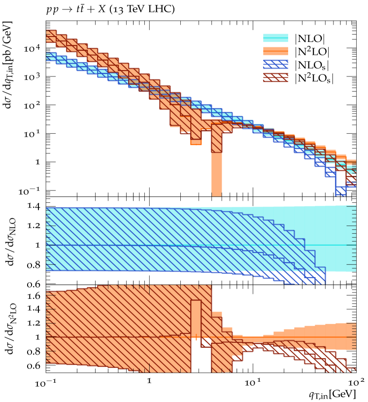
(a) Numeric results of ${\rm d}\sigma_{{t{\bar{t}}}}/{\rm d}q_{\mathrm{T,in}}$

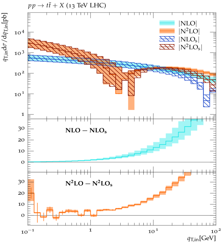
(b) Numeric results of ${\rm d}\sigma_{{t{\bar{t}}}}/{\rm d}\ln q_{\mathrm{T,in}}$

Figure 5: The fixed-order results of the $q_{\mathrm{T,in}}$ and the weighted $q_{\mathrm{T,in}}$ spectra of the process $pp\to{t{\bar{t}}}+X$ at $\sqrt{s}=13$ TeV. NLO/N²LO represents the differential cross section calculated in the full QCD, while NLO${}_{\text{s}}$/N²LO${}_{\text{s}}$ encodes the leading singular behaviour derived from SCET_II $+$HQET.

In this part, we will confront the differential cross sections derived from the factorisation formula of Eq. (2.43) with those evaluated in the full theory. At this point, it merits reminding that in establishing Eq. (2.43), the asymptotic expansion has been carried out in $\lambda_{\tau}$ by means of the region expansion of [78, 79, 80, 81], and only the leading singular contributions have been taken into account in the approximate outputs. In order to assess the effectiveness of this approximation, and in turn the resummation scheme of Eqs. (3.14)-(3.16), it is of the crucial importance for this work to compare the numeric performances of the exact and approximate spectra in the asymptotic regime.

Fig. 5 exhibits the calculation of the $q_{\mathrm{T,in}}$ and the weighted $q_{\mathrm{T,in}}$ spectra at NLO and N²LO precision. In the left panel, we focus on the distributions ${\rm d}\sigma^{\mathrm{s}}_{{t{\bar{t}}}}/{\rm d}q_{\mathrm{T,in}}$ and ${\rm d}\sigma^{\mathrm{f.o.}}_{{t{\bar{t}}}}/{\rm d}q_{\mathrm{T,in}}$, in the notation of Sec. 3.4. Please note that while the NLO fixed-order expansions are strictly positive throughout, the N²LO ones are negative at small $q_{\mathrm{T,in}}$ and only return to the positive for $q_{\mathrm{T,in}}\gtrsim 3\,\text{GeV}$. As shown in the top plot, owing to the singular contributions from the asymptotic expansion of Eq. (2.6), the absolute values of the NLO${}_{\text{s}}$ and N²LO${}_{\text{s}}$ results are both in excellent agreement with the exact results in the low $q_{\mathrm{T,in}}$ region. As the value of $q_{\mathrm{T,in}}$ grows, the acuteness of the singular terms becomes gradually alleviated, from which the overall cross-section is reduced. As a result, the NLO${}_{\text{s}}$ and N²LO${}_{\text{s}}$ approximations show progressively larger deviations. The fluctuations visible around $q_{\mathrm{T,in}}=3\,\text{GeV}$ are caused by the slightly different crossing points from the negative to the positive realm of the exact N²LO and approximate N²LO${}_{\text{s}}$ results. At some point, far outside its validity range, the approximate NLO${}_{\text{s}}$ and N²LO${}_{\text{s}}$ again become unphysical, e.g. at $q_{\mathrm{T,in}}\approx 80\,\text{GeV}$ for the NLO${}_{\text{s}}$ results.

Below the main plot, we show two ratios to highlight the relationship between the exact and approximate spectra. Independent of the order of the expansion or the choice on the scale, as indicated by their respective bands, excellent agreement is observed between ${\rm d}\sigma^{\mathrm{s}}_{{t{\bar{t}}}}/{\rm d}q_{\mathrm{T,in}}$ and ${\rm d}\sigma^{\mathrm{f.o.}}_{{t{\bar{t}}}}/{\rm d}q_{\mathrm{T,in}}$ below $q_{\mathrm{T,in}}=1~{}$GeV. Within a few percents of deviation, this holds up to $q_{\mathrm{T,in}}\sim 10~{}$GeV for the NLO${}_{\text{s}}$ bands and $q_{\mathrm{T,in}}\sim 20~{}$GeV in the N²LO${}_{\text{s}}$ results. Further increase in $q_{\mathrm{T,in}}$ will render the power suppressed terms in Eq. (2.6) manifestly important, thereby developing appreciable discrepancies between the QCD and EFT outcomes. For instance, it is seen that in the domain $q_{\mathrm{T,in}}\sim 30\,\text{GeV}$, the leading singular terms only account for about $75\%$ of the NLO and $\sim 80\%$ of the N²LO spectra.

In order to further ascertain the asymptotic properties in the $q_{\mathrm{T,in}}\to 0$ limit, we investigate the $q_{\mathrm{T,in}}$-weighted differential distributions ${\rm d}\sigma_{{t{\bar{t}}}}/{\rm d}\ln q_{\mathrm{T,in}}$ in Fig. 5(b). Akin to Eq. (2.6), the asymptotic expansion can also be applied onto the present case,

$$\frac{{\rm d}{\sigma_{{t{\bar{t}}}}}}{{\rm d}\ln q_{\tau}}\,\sim\;\sigma^{{t{\bar{t}}}}_{\mathrm{B}}\,\sum_{m,n}\,\left[\frac{\alpha_{s}(M_{t{\bar{t}}})}{4\pi}\right]^{m}\,\left[\,\underbrace{c^{(0)}_{m,n}\,{\ln^{n}(\lambda_{\tau})}}_{\mathrm{LP}}+\,\underbrace{c^{(1)}_{m,n}\,\lambda_{\tau}\ln^{n}(\lambda_{\tau})}_{\mathrm{NLP}}+\,\underbrace{c^{(2)}_{m,n}\,\lambda^{2}_{\tau}\ln^{n}(\lambda_{\tau})}_{\mathrm{N}^{2}\mathrm{LP}}+\dots\right]\,.$$ (4.5)

Comparing with Eq. (2.6), the power series of Eq. (4.5) exhibits a less singular behaviour in each order and power in $\lambda_{\tau}$. This characteristic is reflected by the shallower slopes of the NLO${}_{\text{s}}$ and N²LO${}_{\text{s}}$ curves in the main plot of Fig. 5(b). More explicitly, whilst the magnitudes of ${\rm d}\sigma^{\mathrm{s}(\mathrm{f.o.})}_{{t{\bar{t}}}}/{\rm d}\ln q_{\mathrm{T,in}}$ are nearly 10 times smaller than those of ${\rm d}\sigma^{\mathrm{s}(\mathrm{f.o.})}_{{t{\bar{t}}}}/{\rm d}q_{\mathrm{T,in}}$ in the vicinity of $q_{\mathrm{T,in}}=0$, they approach each other when entering the area $q_{\mathrm{T,in}}\sim 10~{}$GeV. On the other hand, differing from Eq. (2.6), the leading power terms of ${\rm d}\sigma_{{t{\bar{t}}}}/{\rm d}\ln q_{\mathrm{T,in}}$ are expected to capture the entire singular behaviour of the spectrum as all subleading power corrections are finite in the limit $q_{\mathrm{T,in}}\to 0$. To verify this property and in turn scrutinise our calculations of the leading singular contributions, the difference between the full theory and the EFT results is addressed in the middle and bottom graphs, at NLO and N²LO accuracy, respectively, of Fig. 5(b). For the NLO${}_{\text{s}}$ results, with the decrease in $q_{\mathrm{T,in}}$, the difference between the full QCD result and our approximation continuously decreases for all scale choices. In particular, in the vicinity of $q_{\mathrm{T,in}}\sim 0.1\,\text{GeV}$, the gaps between the NLO and NLO${}_{\text{s}}$ results shrink to $\sim 0.3~{}$pb, almost a thousand times smaller than the magnitudes of ${\rm d}\sigma^{\mathrm{s}(\mathrm{f.o.})}_{{t{\bar{t}}}}/{\rm d}\ln q_{\mathrm{T,in}}$. We thus conclude that all the singularities of ${\rm d}\sigma^{\mathrm{f.o.}}_{{t{\bar{t}}}}/{\rm d}\ln q_{\mathrm{T,in}}$ at NLO have been successfully incorporated in ${\rm d}\sigma^{\mathrm{s}}_{{t{\bar{t}}}}/{\rm d}\ln q_{\mathrm{T,in}}$. Analogous behaviors can also be found in the N²LO${}_{\text{s}}$ results from the region $q_{\mathrm{T,in}}\geq 2~{}$GeV, where the Monte-Carlo integration errors $\epsilon_{{}_{\mathrm{MC}}}$ for the difference $\text{N${}^{2}$LO}-\text{N${}^{2}$LO${}_{\text{s}}$}$ (indicated by the red bars) are still under control. Further reducing $q_{\mathrm{T,in}}$ leads to growing numerical uncertainties in the calculation of this small residual difference of increasingly large individual weighted cross sections. Nonetheless, numeric zero is still within a few standard deviations $\epsilon_{{}_{\mathrm{MC}}}$ and, thus, the EFT spectra can still be regarded as compatible with the exact results. It should again be stressed that since the absolute values of the N²LO${}_{\text{s}}$ curves are generally above $\mathcal{O}(10^{3})$ within the asymptotic domain, mitigating their absolute uncertainties down to the same level as those in the NLO${}_{\text{s}}$ results necessitates the sub-permille relative accuracy in running the programs, which is rather demanding in time and thus has to be postponed to future research.

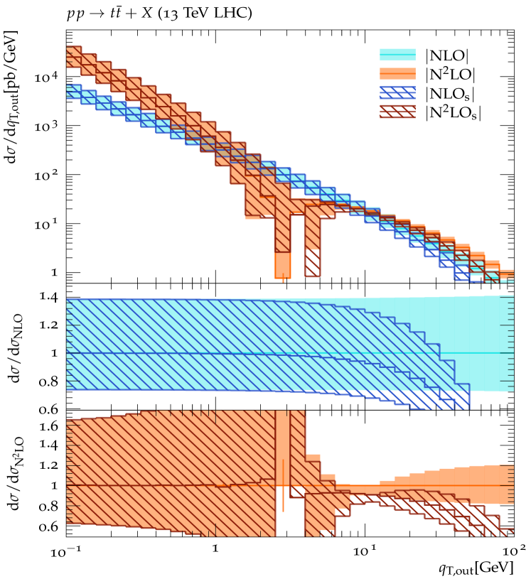
(a) Numeric results of ${\rm d}\sigma_{{t{\bar{t}}}}/{\rm d}q_{\mathrm{T,out}}$

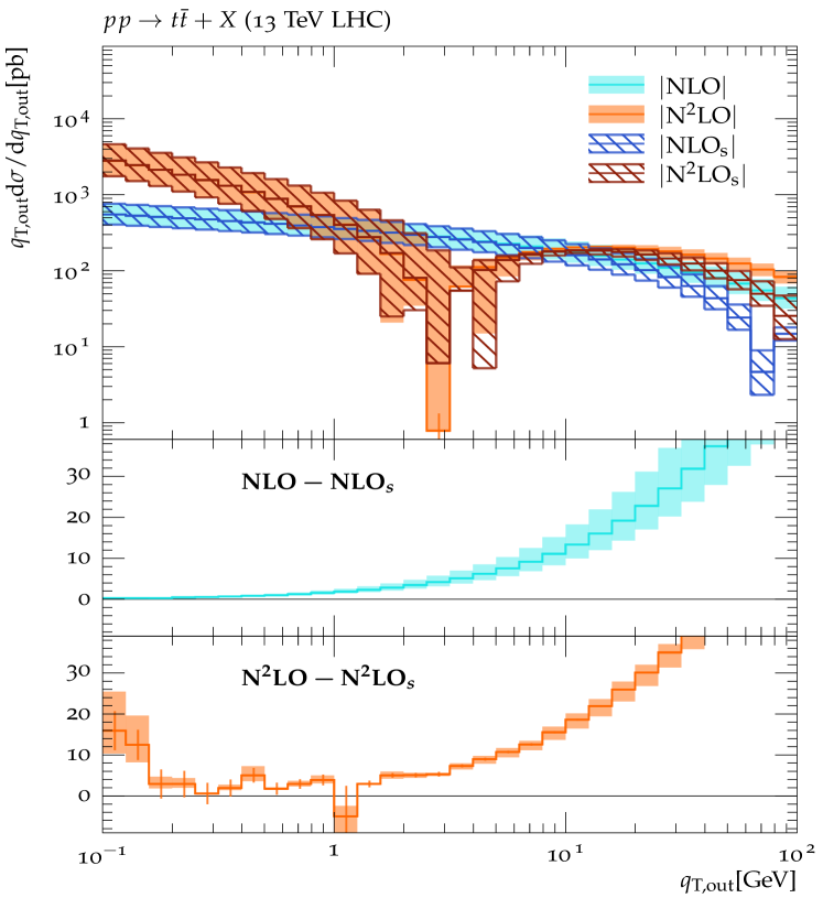
(b) Numeric results of ${\rm d}\sigma_{{t{\bar{t}}}}/{\rm d}\ln q_{\mathrm{T,out}}$

Figure 6: The fixed-order results of the $q_{\mathrm{T,out}}$ and the weighted $q_{\mathrm{T,out}}$ spectra of the process $pp\to{t{\bar{t}}}+X$ at $\sqrt{s}=13$ TeV. NLO/N²LO represents the differential cross section calculated in the full QCD, while NLO${}_{\text{s}}$/N²LO${}_{\text{s}}$ encodes the leading singular behaviour derived from SCET_II $+$HQET.

In Fig. 6, we illustrate the fixed-order results of the distributions ${\rm d}\sigma_{{t{\bar{t}}}}/{\rm d}q_{\mathrm{T,out}}$ and ${\rm d}\sigma_{{t{\bar{t}}}}/{\rm d}\ln q_{\mathrm{T,out}}$. Within the asymptotic regime, since the $q_{\mathrm{T,out}}$ observable is subject to the same factorisation formula as that in the $q_{\mathrm{T,in}}$ case, the general pattern of the $q_{\mathrm{T,out}}$ and the weighted spectra are similar to those of Fig. 5. Furthermore, due to the fact that the double-logarithmic terms, induced by the cusp anomalous dimensions in Eq. (3.2) which dominate the leading singular behaviour, are independent of the choice of the reference vector $\vec{\tau}$, the absolute values for ${\rm d}\sigma_{{t{\bar{t}}}}/{\rm d}q_{\mathrm{T,out}}$ and ${\rm d}\sigma_{{t{\bar{t}}}}/{\rm d}\ln q_{\mathrm{T,out}}$ are close to those of $q_{\mathrm{T,in}}$ in Fig. 5. In addition to the top diagrams focusing on the magnitudes of the respective spectra, the lower two panels of Fig. 6 are again dedicated to the comparisons of the exact and approximate results. It is seen that, up to statistical uncertainties, the leading singular terms have suitably reproduced the asymptotic behaviour of the full theory in the small $q_{\mathrm{T,out}}$ domain.

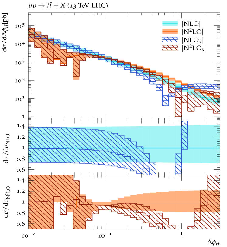
(a) Numeric results of ${\rm d}\sigma_{{t{\bar{t}}}}/{\rm d}\Delta\phi_{{t{\bar{t}}}}$

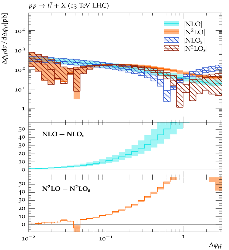
(b) Numeric results of ${\rm d}\sigma_{{t{\bar{t}}}}/{\rm d}\ln\Delta\phi_{{t{\bar{t}}}}$

Figure 7: The fixed-order results of the $\Delta\phi_{{t{\bar{t}}}}$ and the weighted $\Delta\phi_{{t{\bar{t}}}}$ spectra of the process $pp\to{t{\bar{t}}}+X$ at $\sqrt{s}=13$ TeV. NLO/N²LO represents the differential cross section calculated in the full QCD, while NLO${}_{\text{s}}$/N²LO${}_{\text{s}}$ encodes the leading singular behaviour derived from SCET_II $+$HQET.

Fig. 7 finally depicts the results for the ${\rm d}\sigma_{{t{\bar{t}}}}/{\rm d}\Delta\phi_{{t{\bar{t}}}}$ and ${\rm d}\sigma_{{t{\bar{t}}}}/{\rm d}\ln\Delta\phi_{{t{\bar{t}}}}$ spectra. Taking into account the facts that the azimuthal distributions are in practice derived from the $q_{\mathrm{T,out}}$ spectrum by means of Eq. (3.22) and also that the contributions from the region $\vec{P}_{t}^{\perp}\sim\mathcal{O}(10^{2})\,\text{GeV}$ provide the bulk of the cross section [27, 28], we find that the ${\rm d}\sigma_{{t{\bar{t}}}}/{\rm d}\Delta\phi_{{t{\bar{t}}}}$ and ${\rm d}\sigma_{{t{\bar{t}}}}/{\rm d}\ln\Delta\phi_{{t{\bar{t}}}}$ results in the interval $\Delta\phi_{{t{\bar{t}}}}\in[0.01,1]$ of Fig. 7 present a corresponding behaviour to the $q_{\mathrm{T,out}}$ spectra within the $q_{\mathrm{T,out}}\in[1,100]\,\text{GeV}$ region of Fig. 6. For example, the NLO${}_{\text{s}}$ curves intercept the N²LO${}_{\text{s}}$ ones around $\Delta\phi_{{t{\bar{t}}}}=0.01$ and $\Delta\phi_{{t{\bar{t}}}}=0.1$ in Fig. 7, while similar intercepts also take place close to $q_{\mathrm{T,out}}=1\,\text{GeV}$ and $q_{\mathrm{T,out}}=10\,\text{GeV}$ in Fig. 6. Finally, as before, Fig. 7 delivers the ratios of the $\Delta\phi_{{t{\bar{t}}}}$ spectra as well as the differences of the weighted $\Delta\phi_{{t{\bar{t}}}}$ distributions, to compare the approximate and exact spectra. As before, except for the calculations crossing from negative to positive cross sections in the vicinity of $\Delta\phi_{{t{\bar{t}}}}\sim 0.03$ of Fig. 7(a) and the numerical instability observed at $\Delta\phi_{{t{\bar{t}}}}\sim 0.04$ in Fig. 7(b), we observe excellent agreement in the asymptotic domain $\Delta\phi_{{t{\bar{t}}}}\lesssim 0.1$.

4.3 Resummation improved results

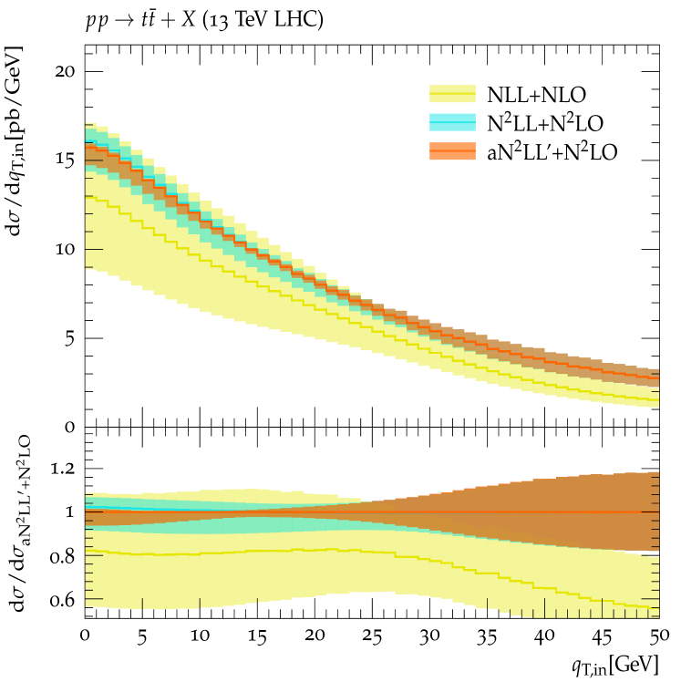
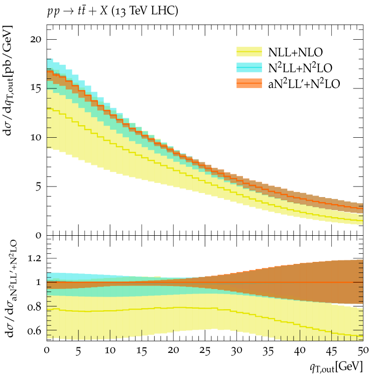
Figure 8: The resummation improved spectra of $q_{\mathrm{T,in}}$ and $q_{\mathrm{T,out}}$ at NLL+NLO, N²LL+N²LO, and approximate N²LL^′+N²LO accuracies (aN²LL^′+N²LO).

We now match our resummed calculation, validated in the previous section, to the exact fixed-order result, according to Eq. (3.23). To facilitate our calculations of the exact spectra, lower cutoffs in the respective observable have been implemented as shown in Eq. (4.1). They are justified by the above findings, namely the agreement of the fixed-order expansion of the approximation and the full QCD calculation, in the asymptotic domain. It is important to note that the full theory calculation participates in the matching procedure through the ratio $\mathcal{R}_{\mathrm{fs}}$ defined in Eq. (3.28). As illustrated in Figs. 5(a), 6(a), and 7(a), this ratio approaches unity in the asymptotic region for all observables investigated in this paper. Consequently, for practical evaluations, we are justified to truncate the impact of the full theory below the boundaries in Eq. (4.1). Further lowering these boundaries in principle helps to suppress the power corrections, which however entails much longer run time of our programs.

The other major ingredient in our matching procedure is the transition function $f_{\mathrm{tran}}$ which, together with the shape parameters $\{c_{\rm{m}},r_{\mathrm{m}}\}$, governs the active range of the resummation. In light of the excellent agreement between QCD and EFT, see Figs. 5-7, the chosen default values of $\{c_{\rm{m}},r_{\mathrm{m}}\}$ are given in Eq. (3.26) and Eq. (3.27). The transition function ensures that the resummation of Eq. (3.14) is fully operational in the asymptotic regions. In the present paper, we choose these regions to be $q_{\mathrm{T,in(out)}}\leq 10\,\text{GeV}$ and $\Delta\phi_{{t{\bar{t}}}}\leq 0.1$. The contribution of the resummation to the matched result is then continuously reduced, reaching half its intrinsic value at the focal point $c_{\mathrm{m}}$, 30 GeV in the $q_{\mathrm{T,in(out)}}$ spectra and 0.3 in the $\Delta\phi_{{t{\bar{t}}}}$ spectrum. The resummation is eventually fully switched off for $\mathcal{Q}\geq c_{\mathrm{m}}+r_{\mathrm{m}}$, $50\,\text{GeV}$ for $\mathcal{Q}=q_{\mathrm{T,in(out)}}$ and $0.5$ for $\mathcal{Q}=\Delta\phi_{{t{\bar{t}}}}$. Alternative settings for $c_{\mathrm{m}}$ and $r_{\mathrm{m}}$, see Eq. (4.3) and Eq. (4.4), are assessed to estimate the associated theoretical uncertainty of the matching processes.

In Fig. 8, we present the resummation improved differential cross sections ${\rm d}\sigma_{{t{\bar{t}}}}/{\rm d}q_{\mathrm{T,in}}$ and ${\rm d}\sigma_{{t{\bar{t}}}}/{\rm d}q_{\mathrm{T,out}}$. Within the small $q_{\mathrm{T,in(out)}}$ regimes, in contrast to the fixed-order results of Figs. 5(a)-7(a), where substantial N²LO contributions were observed, the resummed spectra here have been stabilised at the respective accuracies. Especially, a reduction in the theoretical uncertainties, detailed through their respective coloured bands, can be found with the increase in the logarithmic accuracy. For example, in the limits $q_{\mathrm{T,in}}\to 0$ and $q_{\mathrm{T,out}}\to 0$, the results on the aN²LL^′+N²LO level, that constitute our best prediction, possess relative uncertainties of about ${+1\%}$ and ${-5\%}$. They are greatly reduced from the uncertainties of the N²LL+N²LO calculations, being from $+6\%$ to $-12\%$. For illustrational purposes we also include the lowest order NLL+NLO calculation showing uncertainties of $\pm 30\%$. The primary driver behind those theoretical uncertainties is the variation of the beam scale $\mu_{b}$.

On the other hand, as exhibited in Fig. 8, the central values in higher precision are in general contained in the uncertainty bands at the lower accuracy and in particular, the central result of N²LL+N²LO almost coincides with that at aN²LL^′+N²LO. At this point, it merits reminding that with our default choice in Eq. (3.17), the logarithmic contributions from the fixed order functions are all diminished, such that the discrepancy between N²LL+N²LO and aN²LL^′+N²LO central curves is determined by the constant terms, which, in our case, are those from the beam sectors only. Further inclusion of the N²LO constant terms from the hard and soft ingredients may alter this difference, which nevertheless has to be verified by an exact N²LL^′+N²LO calculation.

Departing from the asymptotic regime, the curves in Fig. 8 enter transitional period ranging from $q_{\mathrm{T,in(out)}}=25~{}$GeV to $q_{\mathrm{T,in(out)}}=35~{}$GeV, where the error bands are progressively aligning as the different resummations are faded out and the fixed order contributions, which are the same in the N²LL+N²LO and aN²LL^′+N²LO calculations, gradually take over. The cause for the uncertainties in this interval is multifaceted, comprising the variation of the beam scale $\mu_{b}$, the fixed order scale $\mu_{\mathrm{f.o.}}$, and the reshaping of the transition function $f_{\mathrm{tran}}$ through the inputs $\{c_{m},r_{m}\}$. Further increasing the magnitudes of $q_{\mathrm{T,in(out)}}$ dives into the tail domain, where the central values of the respective spectra are dominated by the fixed order results and the uncertainties therein are ruled by the sensitivity to the scale $\mu_{\mathrm{f.o.}}$. Improving the theoretical uncertainties at this moment is out of the scope of resummation and entails a full N³LO QCD calculation of $pp\to t\bar{t}+X$.

Comparing the spectra of $q_{\mathrm{T,in}}$ with the $q_{\mathrm{T,out}}$ ones, it is interesting to find that their NLL+NLO results are in close agreement with each other, whereas those at N²LL+N²LO or aN²LL^′+N²LO accuracy start to exhibit larger differences. In particular, the $q_{\mathrm{T,out}}$ spectra are raised by $\approx 1~{}$pb/GeV with regard to the $q_{\mathrm{T,in}}$ one in the asymptotic regime. To interpret this, it is beneficial to remind that according to Tab. 1, the NLL resummation only involves the evolution kernels $\mathcal{D}^{\mathrm{res}}_{[\kappa]}$ and $\mathcal{V}^{[\kappa]}$ in Eqs. (3.15)-(3.16), both of which, as defined in Eq. (3.2) and Eq. (B.3), concern only the magnitude of $\vec{b}_{\tau_{\|}}$ and thus fail to differentiate between the $q_{\mathrm{T,out}}$ and $q_{\mathrm{T,in}}$ observables. However, starting from N²LL, the $\vec{\tau}$-dependent components, such as the soft function $\mathcal{S}_{[\kappa]}$ and the gluon beam sector $\mathcal{B}^{[g_{n(\bar{n})}]}$, come into play, thus including a non-trivial impact that the projected direction $\vec{\tau}$ can make on the results.

Furthermore, contrary to the azimuthally averaged transverse momentum distributions calculated in [68, 65], no Sudakov peak is formed in the projected transverse momentum case, as displayed in Fig. 8. This originates in part from the kinematic differences of these two observables. In the R(a)GE framework introduced in Sec. 3.2, the resummed $q_{\mathrm{T}}$ distributions can be addressed as,

$$\frac{{\rm d}\sigma_{{t{\bar{t}}}}}{{\rm d}q_{\mathrm{T}}}\,\sim\;q_{\mathrm{T}}\,\sum_{\kappa}\,\int{\rm d}\vec{b}_{\mathrm{T}}\,J_{0}(b_{\mathrm{T}}q_{\mathrm{T}})\,\widetilde{\Sigma}^{\mathrm{res},[\kappa]}_{{t{\bar{t}}}}(\vec{b}_{\mathrm{T}},M_{t{\bar{t}}},\beta_{t{\bar{t}}},x_{t},Y_{t{\bar{t}}})\,,$$ (4.6)

where $J_{0}$ stands for the zeroth-rank Bessel function. Taking the limit $q_{\mathrm{T}}\to 0$, while the integrand in Eq. (4.6) approaches a constant value, the pre-factor $q_{\mathrm{T}}$ linearly suppresses the resummed spectra, which in turn leads to the formation of a Sudakov peak. Such a linear factor is absent for $q_{\mathrm{T,in}}$ and $q_{\mathrm{T,out}}$. As formulated in Eq. (3.14), the situation of the $q_{\tau}$ resummation is

$$\frac{{\rm d}\sigma_{{t{\bar{t}}}}}{{\rm d}q_{\tau}}\,\sim\;\sum_{\kappa}\int{\rm d}b_{\tau_{\|}}\,\cos(b_{\tau_{\|}}q_{\tau})\,\widetilde{\Sigma}^{\mathrm{res},[\kappa]}_{{t{\bar{t}}}}(b_{\tau_{\|}}\vec{\tau},M_{t{\bar{t}}},\beta_{t{\bar{t}}},x_{t},Y_{t{\bar{t}}})\,.$$ (4.7)

Thus, the $q_{\tau}$ spectra here receive no kinematical suppressions in the asymptotic limit, explaining the absence of the Sudakov peaks in Fig. 8.

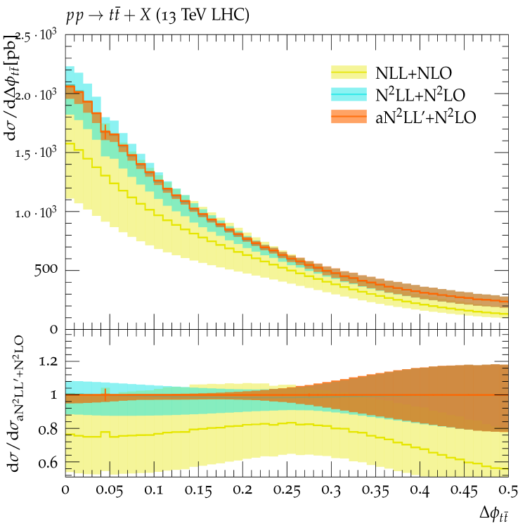
Figure 9: The resummation improved azimuthal spectra ${\rm d}\sigma_{{t{\bar{t}}}}/{\rm d}\Delta\phi_{{t{\bar{t}}}}$ at NLL+NLO, N²LL+N²LO, and approximate N²LL^′+N²LO accuracies (aN²LL^′+N²LO).

Finally, in Fig. 9, we show the resummation improved azimuthal separations between the top and anti-top quarks. Since at the leading power, the observable $\Delta\phi_{{t{\bar{t}}}}$ exhibits the same factorisation and resummation patterns as the $q_{\mathrm{T,out}}$ and $q_{\mathrm{T,in}}$ spectra, the curves from Fig. 9 present analogous behaviors to the ones in Fig. 8, including the converging theoretical uncertainties with the increasing of the precision of the calculation. Due to the same reasons as before, a Sudakov peak cannot be observed in the asymptotic domain. In particular, the latter case appears to be in conflict with the finding in a similar observable in Drell-Yan production [204] where Sudakov peaks were observed in the azimuthal spectra. This contradiction is, however, found to be spurious. The constraints on the transverse momentum that had been imposed on the final state in [204] through fiducial cuts and the projection of the observable into multiple transverse momentum slices introduced an effective kinematic damping factor through the shrinking phase space, thereby restoring a similar Sudakov peak structure as observed in the azimuthally averaged transverse momentum distribution of [204]. On the contrary, despite requiring $M_{t{\bar{t}}}\geq 400\,\text{GeV}$ in this paper and the prefactor $\vec{P}^{\perp}_{t}$ having emerged from the expansions in Eq. (3.22), neither of them can collapse the phase space for $\Delta\phi_{{t{\bar{t}}}}\to 0$ sufficiently for such a structure to emerge.

5 Conclusions

In this paper, we investigated the projected transverse momentum spectrum $q_{\tau}$, which can be evaluated by integrating out the rejection components of $\vec{q}_{\mathrm{T}}$ with respect to the reference unit vector $\vec{\tau}$. We focussed on its singular behaviour in the low $q_{\tau}$ domain in particular.

Using the region expansion methods [78, 79, 80, 81] we resolved the phase space and loop integrals in terms of the dynamic regions that capture the asymptotic properties of ${\rm d}\sigma_{{t{\bar{t}}}}/{\rm d}q_{\tau}$ in the vicinity of $q_{\tau}=0$. It comprises the usual hard, beam-collinear, jet-collinear, and soft domains. Then, in the context of the effective field theories, SCET_II and HQET, we enumerated the possible configurations constructed by those momentum modes, and determined the power accuracy in each case by probing the corresponding factorisation formulae. It is observed that the leading singular terms of the $q_{\tau}$ distribution are governed by the hard, beam-collinear, and soft regions, akin to the $q_{\mathrm{T}}$ spectrum [64, 65, 66, 67, 68, 74], whilst the higher power regular terms entail the participations of the jet-collinear regime.

In the subsequent resummation, we focussed on the leading asymptotic behaviour of ${\rm d}\sigma_{{t{\bar{t}}}}/{\rm d}q_{\tau}$. By inspecting the corresponding factorisation formula in impact space, we illustrated that the driving factor of the singular behaviour in momentum space is the characteristic logarithm $\ln^{k}[{{b}^{2}_{\tau_{\|}}M_{t{\bar{t}}}^{2}}/{b_{0}^{2}}]$, for $k\geq 1$, which therefore permitted us to apply the framework of RGE and RaGE [96, 97, 98, 99] to accomplish the logarithmic exponentiation and in turn the resummation. It is worth emphasizing that in presence of the azimuthal asymmetric terms, this phenomenon is not general on the process $pp\to{t{\bar{t}}}+X$. The $q_{\tau}$ spectra and the azimuthally averaged case ${\rm d}\sigma_{{t{\bar{t}}}}/{\rm d}q_{\mathrm{T}}$ are known to be the only two observables which stem from the double-differential distribution ${\rm d}\sigma_{{t{\bar{t}}}}/{\rm d}q_{\mathrm{T}}$ but are free of the azimuthal asymmetric divergences.

Although the derivation and findings summarised above hold for an arbitrary choice of reference vector $\vec{\tau}$, we focussed on three specific observables to demonstrate the validity and usefulness of our framework, $q_{\mathrm{T,in}}$, $q_{\mathrm{T,out}}$, and $\Delta\phi_{{t{\bar{t}}}}$. The first two cases are obtained by assigning $\vec{\tau}$ to be parallel and perpendicular with respect to the transverse momentum of the top quark, respectively. The azimuthal spectrum ${\rm d}\sigma_{{t{\bar{t}}}}/{\rm d}\Delta\phi_{{t{\bar{t}}}}$ is extracted from ${\rm d}\sigma_{{t{\bar{t}}}}/{\rm d}q_{\mathrm{T,out}}$ according to the kinematical relationship in between. Owing to the independence from azimuthally asymmetric divergences, we were able to calculate those observables at NLL+NLO, N²LL+N²LO, and approximate N²LL^′+N²LO (aN²LL^′+N²LO) accuracy. From the numerical results, a manifest perturbative convergence is observed in the asymptotic regime, i.e. the central values at the higher precisions are generally contained in the uncertainty bands of the lower ones and the respective uncertainties are systematically reduced down to the percent level at aN²LL^′+N²LO. During our calculation, we have focussed on the domain $M_{t\bar{t}}\geq 400~{}$GeV to evade Coulomb divergences which inevitably manifest themselves in the higher order corrections. It is expected that our results can be compared against the very recent measurement on the double differential spectra ${\rm d}\sigma_{{t{\bar{t}}}}/({\rm d}M_{t{\bar{t}}}\,{\rm d}\Delta\phi_{{t{\bar{t}}}})$ [21] within the corresponding $M_{t{\bar{t}}}$ slices upon the full publication of the experimental data. To expand our results to the full phase space, including the threshold regime $M_{t{\bar{t}}}<400~{}$GeV, the emergence of Coulomb singularities at the ${t{\bar{t}}}$ production threshold necessitates a combined resummation of the beam-collinear, soft, and Coulomb interactions, which we seek to address in a future publication.

Acknowledgements

WJ is grateful to Jean-Nicolas Lang for providing detailed instructions on the usage of R ECOLA . WJ also would like to thank L. Chen, M. Czakon and R. Poncelet for the helpful discussions on the N²LO hard function. This work is supported by a Royal Society through a University Research Fellowship (URF\R1\180549) and an Enhancement Award (RGF\EA\181033, CEC19\100349, and RF\ERE\210397).

Appendix A The double differential transverse momentum distribution ${\rm d}^{2}\sigma_{{t{\bar{t}}}}/{\rm d}^{2}\vec{q}_{\mathrm{T}}$

As discussed in Sec. 3.1, in absence of the azimuthal asymmetric term (AAT), the main task in resumming the singular behaviors on the $q_{\tau}$ spectra is to exponentiate the characteristic logarithmic terms in impact space. Nevertheless, in light of the non-trivial contributions of the helicity-flipping beam functions as well as the soft correlations, the resummation of a general observable is more complicated. Hence, this appendix will calculate the double differential spectrum as an example to illustrate the effect of the AATs on the fixed-order expansion and the organisation of the logarithmic terms. Alternative cases with active AATs contributions can also be found in [72, 73, 66, 67, 206, 207, 208, 209].

Considering that the contributions to the $\vec{q}_{\mathrm{T}}$ distributions from the hard jet regions, $N_{\mathrm{J}}\geq 1$, have been demonstrated to be power suppressed [74, 131], the factorisation formula is now subject to only the $N_{\mathrm{J}}=0$ configuration at leading power. Therefore, they can be extracted from Eq. (2.26) after reducing the heavy parton correlation functions with Eqs. (2.27)-(2.28). It follows that,

$$\frac{{\rm d}{\sigma_{{t{\bar{t}}}}}}{{\rm d}M_{t{\bar{t}}}^{2}\,{\rm d}^{2}\vec{P}_{t}^{\perp}\,{\rm d}Y_{t{\bar{t}}}\,{\rm d}^{2}\vec{q}_{\mathrm{T}}}=\sum_{\mathrm{sign}[x_{t}]}\sum_{\kappa}\,\frac{\Theta_{\mathrm{kin}}^{(0)}}{64\pi^{4}\,\beta_{t{\bar{t}}}\,|x_{t}|\,M_{t{\bar{t}}}^{4}\,s}\,\int{\rm d}^{2}\vec{b}_{\mathrm{T}}\,\exp\left(\vec{q}_{\mathrm{T}}\cdot\vec{b}_{\mathrm{T}}\right)\,\widetilde{\Sigma}_{{t{\bar{t}}}}^{[\kappa]}(\vec{b}_{\mathrm{T}},M_{t{\bar{t}}},\beta_{t{\bar{t}}},x_{t},Y_{t{\bar{t}}})\,,$$ (A.1)

where $\kappa\in\{g_{n}g_{\bar{n}},q^{i}_{n}\bar{q}^{j}_{\bar{n}},q^{i}_{\bar{n}}\bar{q}^{j}_{n}\}$ again denotes the partonic channel. The constituents of $\widetilde{\Sigma}_{{t{\bar{t}}}}^{[\kappa]}$ have been specified in Eqs. (2.29)-(2.30) for each partonic channel. Upon the usage of the identities in Eqs. (2.27)-(2.28), Eq. (A.1) inherits the problems from Coulomb exchanges as well, akin to Eq. (2.43). To this end, we will constrain the following investigation within the domain $M_{t{\bar{t}}}\geq 400\,\text{GeV}$, or equivalently, $\beta_{t{\bar{t}}}\gtrsim 0.5$, to circumvent the threshold regime.

Generically, the expressions of $\widetilde{\Sigma}^{[\dots]}_{{t{\bar{t}}}}$ at an arbitrary order in $\alpha_{s}$ can be parameterized as

$$\widetilde{\Sigma}^{[\dots]}_{{t{\bar{t}}}}\,\sim\;\sum_{m,n}\,\alpha^{m}_{s}(M_{t{\bar{t}}})\,L_{\mathrm{T}}^{n}\,\Big{\{}s_{m}(\beta_{t{\bar{t}}},x_{t},Y_{t{\bar{t}}})+a_{m}(\widehat{b}_{\mathrm{T}},\beta_{t{\bar{t}}},x_{t},Y_{t{\bar{t}}})\Big{\}}\,,$$ (A.2)

where $L_{\mathrm{T}}\equiv\log\left[{b_{\mathrm{T}}^{2}M_{t{\bar{t}}}^{2}}/{b_{0}^{2}}\right]$ and $\widehat{b}_{\mathrm{T}}\equiv\vec{b}_{\mathrm{T}}/b_{\mathrm{T}}$. The dimensionless coefficients $s_{m,n}$ and $a_{m,n}$ encode the azimuthal symmetric and asymmetric contributions, respectively. Substituting Eq. (A.2) into Eq. (A.1) permits us to evaluate the impact space integrals, namely,

$$\frac{{\rm d}{\sigma_{{t{\bar{t}}}}}}{{\rm d}M_{t{\bar{t}}}^{2}\,{\rm d}^{2}\vec{P}_{t}^{\perp}\,{\rm d}Y_{t{\bar{t}}}\,{\rm d}^{2}\vec{q}_{\mathrm{T}}}\,\sim\;\sum_{m,n}\alpha^{m}_{s}(M_{t{\bar{t}}})\Bigg{\{}s_{m,n}(\beta_{t{\bar{t}}},x_{t},Y_{t{\bar{t}}})\,\mathcal{F}^{(n)}_{\mathrm{T}}(q_{\mathrm{T}},M_{t{\bar{t}}})+\mathcal{A}^{(n)}_{\mathrm{T}}\Big{[}\vec{q}_{\mathrm{T}},M_{t{\bar{t}}},a_{m,n}\Big{]}\Bigg{\}}\,.$$ (A.3)

Herein, since the ASTs are all independent of the impact parameter $\vec{b}_{\mathrm{T}}$, we can factor them out of the $\vec{b}_{\mathrm{T}}$-integrals and apply the inverse Fourier transformations only onto the logarithmic terms, i.e.

$$\mathcal{F}^{(n)}_{\mathrm{T}} (q_{\mathrm{T}},M_{t{\bar{t}}})\,=\;\int{\rm d}^{2}b_{\mathrm{T}}\,\exp\left(\vec{q}_{\mathrm{T}}\cdot\vec{b}_{\mathrm{T}}\right)\,L^{n}_{\mathrm{T}}\,.$$ (A.4)

The calculation of $\mathcal{F}^{(n)}_{\mathrm{T}}$ follows a similar pattern to Eq. (3.1). The corresponding generating function now reads [102],

$$\mathbf{F}_{\mathrm{T}}(\eta,q_{\mathrm{T}},M_{t{\bar{t}}})\,= \;\sum_{n}\frac{\eta^{n}}{n!}\,\mathcal{F}^{(n)}_{\mathrm{T}}(q_{\mathrm{T}},M_{t{\bar{t}}})\,=\;\int{\rm d}^{2}\vec{b}_{\mathrm{T}}\,\exp\left(\vec{q}_{\mathrm{T}}\cdot\vec{b}_{\mathrm{T}}\right)\,\left(\frac{b_{\mathrm{T}}^{2}M_{t{\bar{t}}}^{2}}{b_{0}^{2}}\right)^{\eta}$$

$$\,= \;\frac{4\pi e^{2\gamma_{\mathrm{E}}\eta}}{q_{\mathrm{T}}^{2}}\,\frac{\Gamma[1+\eta]}{\Gamma[-\eta]}\,\left(\frac{M_{t{\bar{t}}}^{2}}{q_{\mathrm{T}}^{2}}\right)^{\eta}\,.$$ (A.5)

$\mathcal{F}^{(n)}_{\mathrm{T}}$ can be extracted by expanding $\mathbf{F}_{\mathrm{T}}(\eta,q_{\mathrm{T}},M_{t{\bar{t}}})$ in $\eta$ as appropriate. The expressions of the first few ranks are

$$\mathcal{F}^{(0)}_{\mathrm{T}}(q_{\mathrm{T}},M_{t{\bar{t}}}) =0\,,$$ (A.6)

$$\mathcal{F}^{(1)}_{\mathrm{T}}(q_{\mathrm{T}},M_{t{\bar{t}}}) =-\frac{4\pi}{q_{\mathrm{T}}^{2}}\,,$$ (A.7)

$$\mathcal{F}^{(2)}_{\mathrm{T}}(q_{\mathrm{T}},M_{t{\bar{t}}}) =-\frac{8\pi}{q_{\mathrm{T}}^{2}}\ln\left[\frac{M_{t{\bar{t}}}^{2}}{q_{\mathrm{T}}^{2}}\right]\,,$$ (A.8)

$$\;\,\vdots$$

From Eq. (A.6) it is seen that the ASTs themselves cannot induce any asymptotic behaviour in the small $q_{\mathrm{T}}$ domain, whilst the logarithmic term $L_{\mathrm{T}}^{m}$ $(m\geq 1)$ is able to produce singular contributions up to $\ln^{m-1}[M_{t{\bar{t}}}^{2}/q_{\mathrm{T}}^{2}]/q_{\mathrm{T}}^{2}$ after completing the inverse Fourier transformations. This observation is found by analogy with Eq. (3.5) and also the circumstances of the azimuthally averaged observables in [68, 64, 65].

On the other hand, Eq. (A.3) also includes contributions from the AATs $a_{m,n}$. In light of their explicit dependence on the orientation of $\vec{b}_{\mathrm{T}}$, the inverse Fourier transformation now comprises both $a_{m,n}$ and $L^{n}_{\mathrm{T}}$, that is,

$$\mathcal{A}^{(n)}_{\mathrm{T}}\Big{[}\vec{q}_{\mathrm{T}},M_{t{\bar{t}}},A\Big{]}\,=\;\int{\rm d}^{2}b_{\mathrm{T}}\,\exp\left(\vec{q}_{\mathrm{T}}\cdot\vec{b}_{\mathrm{T}}\right)\,L^{n}_{\mathrm{T}}\,A(\phi_{qb})\,,$$ (A.9)

where $A(\phi_{qb})$ represents a generic function of the azimuthal difference $\phi_{qb}$ between the vector $\vec{b}_{\mathrm{T}}$ and $\vec{q}_{\mathrm{T}}$, which thereafter participates in the functional $\mathcal{A}^{(n)}_{\mathrm{T}}$ as one of its arguments. Appraising $\mathcal{A}^{(n)}_{\mathrm{T}}$ will benefit from its generational form as well,

$$\mathbf{A}_{\mathrm{T}}\Big{[}\eta,\vec{q}_{\mathrm{T}},M_{t{\bar{t}}},A\Big{]}\,= \;\sum_{n}\,\frac{\eta^{n}}{n!}\,\mathcal{A}^{(n)}_{\mathrm{T}}\Big{[}\vec{q}_{\mathrm{T}},M_{t{\bar{t}}},A\Big{]}\,=\,\int\,{\rm d}^{2}\vec{b}_{\mathrm{T}}\,\exp\left(\vec{q}_{\mathrm{T}}\cdot\vec{b}_{\mathrm{T}}\right)\,\left(\frac{b_{\mathrm{T}}^{2}M_{t{\bar{t}}}^{2}}{b_{0}^{2}}\right)^{\eta}\,A(\phi_{qb})\,$$

$$\,= \;-\frac{\Gamma[2\eta+2]}{q_{\mathrm{T}}^{2}}\,\frac{e^{2\gamma_{\mathrm{E}}\eta}}{4^{\eta}}\left[\frac{M_{t{\bar{t}}}^{2}}{q_{\mathrm{T}}^{2}}\right]^{\eta}\,\int^{\frac{\pi}{2}}_{0}\,{\rm d}\phi\,\Bigg{\{}c_{\phi}^{-2(1+\eta)}\,e^{\mathrm{i}\pi\eta}\,\bigg{[}A(\phi)-A\Big{(}\frac{\pi}{2}\Big{)}+c_{\phi}A^{\prime}\Big{(}\frac{\pi}{2}\Big{)}\bigg{]}\,$$

$$\;{}+s_{\phi}^{-2(1+\eta)}\,e^{-\mathrm{i}\pi\eta}\,\bigg{[}A\Big{(}\phi+\frac{\pi}{2}\Big{)}-A\Big{(}\frac{\pi}{2}\Big{)}-s_{\phi}A^{\prime}\Big{(}\frac{\pi}{2}\Big{)}\bigg{]}+c_{\phi}^{-2(1+\eta)}\,e^{-\mathrm{i}\pi\eta}\bigg{[}A\Big{(}\phi+\pi\Big{)}\,$$

$$\;{}-A\Big{(}\frac{3\pi}{2}\Big{)}+c_{\phi}A^{\prime}\Big{(}\frac{3\pi}{2}\Big{)}\bigg{]}+s_{\phi}^{-2(1+\eta)}\,e^{\mathrm{i}\pi\eta}\,\bigg{[}A\Big{(}\phi+\frac{3\pi}{2}\Big{)}-A\Big{(}\frac{3\pi}{2}\Big{)}-s_{\phi}A^{\prime}\Big{(}\frac{3\pi}{2}\Big{)}\bigg{]}\Bigg{\}}\,$$

$$\;{}-\sqrt{\pi}\,\frac{\Gamma[2\eta+2]}{q_{\mathrm{T}}^{2}}\frac{e^{2\gamma_{\mathrm{E}}\eta}}{4^{\eta}}\left[\frac{M_{t{\bar{t}}}^{2}}{q_{\mathrm{T}}^{2}}\right]^{\eta}\,\Bigg{\{}\frac{\cos(\pi\eta)\Gamma[-\frac{1}{2}-\eta]}{\Gamma[-\eta]}\bigg{[}A\Big{(}\frac{\pi}{2}\Big{)}+A\Big{(}\frac{3\pi}{2}\Big{)}\bigg{]}\,$$

$$\;{}-\frac{\mathrm{i}\sin(\pi\eta)\Gamma[-\eta]}{\Gamma[\frac{1}{2}-\eta]}\bigg{[}A^{\prime}\Big{(}\frac{\pi}{2}\Big{)}-A^{\prime}\Big{(}\frac{3\pi}{2}\Big{)}\bigg{]}\Bigg{\}}\,,$$ (A.10)

where $c_{\phi}=\cos(\phi)$ and $s_{\phi}=\sin(\phi)$. In deriving Eq. (A), the function $A(\phi_{qb})$ is assumed to be analytically continuous in the entire domain $\phi_{qb}\in[0,2\pi]$, and the result is expected to be applicable to any azimuthal asymmetric contributions that stem from the beam functions, the soft sectors, or the products of these two cases. In the following discussion, we will focus on scenarios of the beam constituent. The other two pieces observe the same scaling manner but incur lengthier expressions.

As defined in Eq. (2.36), the gluon beam function constitutes a $2\times 2$ matrix in the helicity space. With the choice of helicity bases of Eq. (2.37), while the diagonal entries characterise the ASTs, the off-diagonal ones, which are always proportional to $e^{\pm\mathrm{i}2\phi_{tb}}$, encode the azimuthal asymmetric contributions, namely, $A(\phi_{qb})\propto e^{\pm\mathrm{i}2(\phi_{qb}+\phi_{tq})}$. Here $\phi_{tb}$ ($\phi_{tq}$) signifies the azimuthal difference between the top quark with respect to the vector $\vec{b}_{\mathrm{T}}$ ($\vec{q}_{\mathrm{T}}$). Plugging this expression into Eq. (A) and then performing the expansions in $\eta$, it yields,

$$\mathcal{A}^{(0)}_{\mathrm{T}}\Big{[}\vec{q}_{\mathrm{T}},M_{t{\bar{t}}},e^{\pm\mathrm{i}2(\phi_{qb}+\phi_{tq})}\Big{]}\,= \;-\frac{4\pi}{q_{\mathrm{T}}^{2}}\,e^{\pm\mathrm{i}2\phi_{tq}}\,,$$ (A.11)

$$\mathcal{A}^{(1)}_{\mathrm{T}}\Big{[}\vec{q}_{\mathrm{T}},M_{t{\bar{t}}},e^{\pm\mathrm{i}2(\phi_{qb}+\phi_{tq})}\Big{]}\,= \;-\frac{4\pi}{q_{\mathrm{T}}^{2}}\,\bigg{\{}\ln\left[\frac{M_{t{\bar{t}}}^{2}}{q_{\mathrm{T}}^{2}}\right]+1\bigg{\}}\,e^{\pm\mathrm{i}2\phi_{tq}}\,,$$ (A.12)

$$\mathcal{A}^{(2)}_{\mathrm{T}}\Big{[}\vec{q}_{\mathrm{T}},M_{t{\bar{t}}},e^{\pm\mathrm{i}2(\phi_{qb}+\phi_{tq})}\Big{]}\,= \;-\frac{4\pi}{q_{\mathrm{T}}^{2}}\,\bigg{\{}\ln^{2}\left[\frac{M_{t{\bar{t}}}^{2}}{q_{\mathrm{T}}^{2}}\right]+2\ln\left[\frac{M_{t{\bar{t}}}^{2}}{q_{\mathrm{T}}^{2}}\right]\bigg{\}}\,e^{\pm\mathrm{i}2\phi_{tq}}\,,$$ (A.13)

$$\vdots\;$$

It is noted that the situation of $\mathcal{A}^{(m)}_{\mathrm{T}}$ above is quite different from that for the $\mathcal{F}^{(m)}_{\mathrm{T}}$ aforementioned. Firstly, as opposed to Eqs. (A.6)-(A.8), where the logarithmic contribution is the only driver for the singularities in the momentum space, Eq. (A.11) illustrates that the AAT itself can serve as a standalone factor to induce an asymptotic behavior. Secondly, in comparison with Eqs. (A.7)-(A.8), the product of $L^{m}_{\mathrm{T}}$ $(m\geq 1)$ and AATs can induce asymptotic terms up to $\ln^{m}\left[{M_{t{\bar{t}}}^{2}}/{q_{\mathrm{T}}^{2}}\right]/q_{\mathrm{T}}^{2}$, which are stronger than the case of ASTs by one power in $\ln\left[{M_{t{\bar{t}}}^{2}}/{q_{\mathrm{T}}^{2}}\right]$. Thirdly, differing from Eqs. (A.6)-(A.8) concerning only the absolute value of $\vec{q}_{\mathrm{T}}$, the expressions for $\mathcal{A}^{(m)}_{\mathrm{T}}$ additionally depend on the orientation of $\vec{q}_{\mathrm{T}}$ through the phase factor $\exp(\pm 2\phi_{tq})$. It is worth emphasising that even though the gluon beam function is utilised here as an example to derive the $\mathcal{A}^{(m)}_{\mathrm{T}}$s above, as a matter of fact, the phase factor $\exp(\pm k\phi_{tq})$ $(k\in\mathbb{Z})$ can also participate in the soft sectors at an arbitrary perturbative order upon which the spherical harmonics expansion was performed [67]. Given those non-trivial impacts from the AATs, the fixed-order results in the low $q_{\mathrm{T}}$ regime and the subsequent resummation may show a different behaviour from that solely driven by the ASTs. The following paragraphs will take the NLO double differential spectrum ${\rm d}\sigma_{{t{\bar{t}}}}/({\rm d}q_{\mathrm{T}}{\rm d}\Delta\Phi_{tX})$ and its required ingredients for a NLL^′ resummation as examples to elucidate this. Here $\Delta\Phi_{tX}$ stands for the azimuthal separation between the top quark and the total momentum of the emitted partons.

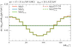
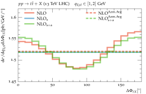
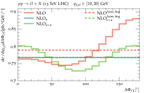
Figure 10: Comparison of the NLO double differential spectra ${\rm d}\sigma_{{t{\bar{t}}}}/({\rm d}q_{\mathrm{T}}{\rm d}\Delta\Phi_{tX})$, shown as distributions of $\Delta\Phi_{tX}$ in slices of $q_{\mathrm{T}}$. Herein, NLO represents the QCD result calculated in S HERPA  [169, 170, 171]. $\text{NLO}_{\mathrm{s}}$ labels the azimuthally symmetric and $\text{NLO}_{\mathrm{s+a}}$ marks the full, i.e. azimuthally symmetric and asymmetric, contributions derived from SCET${}_{\mathrm{II}}+$HQET, respectively. The superscript “$\mathrm{Azm.Avg}$” denotes the azimuthally averaging operation on the exact and approximate spectra.

In Figs. 10-12, we display a comparison of the double differential spectra ${\rm d}\sigma_{{t{\bar{t}}}}/({\rm d}q_{\mathrm{T}}{\rm d}\Delta\Phi_{tX})$ among the exact NLO result, the approximate spectrum NLO_s comprising only the AST contributions, and the full EFT-derived spectrum NLO_s+a including both AST and AAT ingredients. As a first observable, Fig. 10 presents the $\Delta\Phi_{tX}$ distributions, ranging from the parallel configuration, $\Delta\Phi_{tX}=0^{\circ}$, to the opposite one, $\Delta\Phi_{tX}=180^{\circ}$, within three $q_{\mathrm{T}}$ intervals, $q_{\mathrm{T}}\in[0.1,0.2]$ GeV, $q_{\mathrm{T}}\in[1,2]$ GeV, and $q_{\mathrm{T}}\in[10,20]$ GeV. As observed in the left panel of Fig. 10, which focusses on the domain closest to the singularity, $q_{\mathrm{T}}\in[0.1,0.2]$ GeV, the curves of NLO and NLO_s+a are in very good agreement and exhibit a nearly cosinusoidal behaviour on account of the phase factors in Eqs. (A.11)-(A.13) and those stemming from the soft functions. However, if we were to remove the AAT contributions, leaving only the ASTs as active ingredients of our approximation, governed now by Eqs. (A.6)-(A.8) which depend only on the magnitude of $\vec{q}_{\mathrm{T}}$, the resulting curve NLO_s is independent of $\Delta\Phi_{tX}$. After taking the azimuthal averaging operations upon the exact and approximate spectra, however, it is interesting to note that the result of NLO${}^{\mathrm{Azm.Avg}}_{\mathrm{s}+\mathrm{a}}$ coincides with that of NLO_s, and both of them reproduce the exact NLO^Azm.Avg result well. This observation demonstrates that the asymptotic terms in Eqs. (A.11)-(A.13) are indeed able to be eliminated by completing the $\phi_{tq}$ integral, which confirms the discussions in [67] at least at the NLO level. In the centre and right plots of Fig. 10, we move on to the slices $q_{\mathrm{T}}\in[1,2]$ GeV and $q_{\mathrm{T}}\in[10,20]$ GeV. Even though the general patterns herein follow that in the left panel, it is seen that the power corrections gradually become more important with the increase in $q_{\mathrm{T}}$. They give rise to the growing discrepancies between NLO and NLO_s+a results, and also lead to the deviations amid the azimuthally averaged curves.

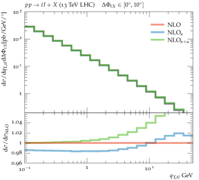
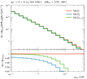
Figure 11: Comparison of the NLO double differential spectra ${\rm d}\sigma_{{t{\bar{t}}}}/({\rm d}q_{\mathrm{T}}{\rm d}\Delta\Phi_{tX})$, shown as distributions of $q_{\mathrm{T}}$ in slices of $\Delta\Phi_{tX}$. Herein, NLO represents the QCD result calculated in S HERPA  [169, 170, 171]. $\text{NLO}_{\mathrm{s}}$ labels the azimuthally symmetric and $\text{NLO}_{\mathrm{s+a}}$ marks the full, i.e. azimuthally symmetric and asymmetric, contributions derived from SCET${}_{\mathrm{II}}+$HQET, respectively.

In Fig, 11, we exhibit the $q_{\mathrm{T}}$ distributions in slices of $\Delta\Phi_{tX}\in[0^{\circ},10^{\circ}]$, $\Delta\Phi_{tX}\in[80^{\circ},100^{\circ}]$, and $\Delta\Phi_{tX}\in[170^{\circ},180^{\circ}]$, which correspond to the peak and trough regions in Fig. 10. We observe that for the majority of the $q_{\mathrm{T}}$ range, the magnitudes of the exact results are close to the approximate calculations NLO_s and NLO_s+a, however, only the NLO_s+a reproduces it well in the region of $q_{\mathrm{T}}\lesssim 1\,$GeV. To interpret this, it is worth noting that at NLO, the most singular terms generated by the ASTs and AATs are $\propto\ln\left[{M_{t{\bar{t}}}^{2}}/{q_{\mathrm{T}}^{2}}\right]/q_{\mathrm{T}}$ and $1/q_{\mathrm{T}}$, respectively. In this regard, the asymptotic behaviors in the low $q_{\mathrm{T}}$ regime are actually dominated by the AST contributions, which therefore is the cause for the nearly coinciding curves in the main plot of Fig. 11. However, it should be stressed that in spite of the minor roles played by AATs, their participations are still of the crucial importance in reproducing the correct singular manner of the exact spectra. As illustrated in the ratio diagrams of Fig. 11, whereas the AST contributions either underestimate or overshoot the NLO results by $\sim 2\%$ in the vicinity of $q_{\mathrm{T}}=0.1~{}$GeV, the curves of NLO_s+a achieve permille level agreement with the exact spectra for all three slices. These phenomena can also be confirmed by Fig. 12, especially in the centre and bottom diagrams therein.

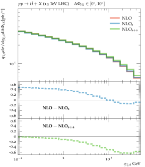
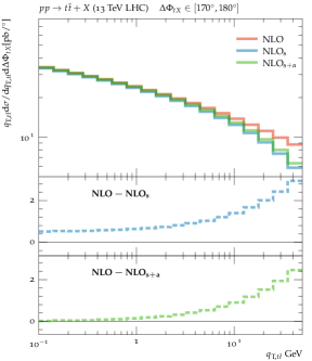
Figure 12: Comparison of the $q_{\mathrm{T}}$-weighted NLO double differential spectra $q_{\mathrm{T}}{\rm d}\sigma_{{t{\bar{t}}}}/({\rm d}q_{\mathrm{T}}{\rm d}\Delta\Phi_{tX})$, shown as distributions of $q_{\mathrm{T}}$ in slices of $\Delta\Phi_{tX}$. Herein, NLO represents the QCD result calculated in S HERPA  [169, 170, 171]. $\text{NLO}_{\mathrm{s}}$ labels the azimuthally symmetric and $\text{NLO}_{\mathrm{s+a}}$ marks the full, i.e. azimuthally symmetric and asymmetric, contributions derived from SCET${}_{\mathrm{II}}+$HQET, respectively.

In light of the non-trivial contributions of the AATs on the leading singular behaviour, the subsequent task is to work out a consistent approach to embed their contributions in the resummation. In circumstances where the singular behaviour is governed solely by the ASTs, the resummation can proceed with exponentiating the characteristic logarithmic terms in the impact space, as discussed in Sec. 3. Considering that the AAT emergence still preserves the factorisation formula and so the according R(a)GEs, we can still apply the logarithmic exponentiation onto the present situation, which then transforms Eq. (A.2) into the following expression,

$$\widetilde{\Sigma}^{[\dots]}_{{t{\bar{t}}}}\,\sim \;\exp\bigg{[}\;L_{\mathrm{T}}\,f_{0}(\alpha_{s}L_{\mathrm{T}})+f_{1}(\alpha_{s}L_{\mathrm{T}})+{\alpha_{s}\,f_{2}(\alpha_{s}L_{\mathrm{T}})}+{\alpha^{2}_{s}\,f_{3}(\alpha_{s}L_{\mathrm{T}})}+\ldots\;\bigg{]}$$

$$\times\,\sum_{m}\,\alpha^{m}_{s}\,\Big{\{}\hat{s}_{m}(\beta_{t{\bar{t}}},x_{t},Y_{t{\bar{t}}})+\hat{a}_{m}(\widehat{b}_{\mathrm{T}},\beta_{t{\bar{t}}},x_{t},Y_{t{\bar{t}}})\Big{\}}\,,$$ (A.14)

where the coefficient functions $f_{k}(k\geq 0)$ are introduced to collect the logarithmic terms at the respective accuracies. $\hat{s}_{m}$ and $\hat{a}_{m}$ stem from the coefficients in Eq. (A.2) capturing the azimuthally symmetric and asymmetric contributions, respectively. In spite of the similar appearance of Eq. (A) to the AST-driven result in Eq. (A.2), it is worth emphasising that the perturbative series in Eq. (A) still possesses the constituents $\hat{a}_{m}$, which can induce a leading asymptotic behaviour after completing the $\vec{b}_{\mathrm{T}}$-integral. To this end, it is of essence to clarify the higher order performance of $\hat{a}_{m}$ so as to determine the subsequent treatments during the resummation. If, akin to the logarithmic contributions in Eqs. (A.6)-(A.8), $\hat{a}_{m}$ invokes deteriorating singularities with the increase in $\alpha_{s}$, a second exponentiating procedure will be necessary to mitigate the theoretical uncertainty caused by the perturbative truncation. Otherwise, after suitable adaptations, we are in principle able to regard the AAT contributions in the similar manner to the ASTs.

To facilitate the discussion, we note that as for an arbitrary order in $\alpha_{s}$, the term $\hat{a}_{m}$ exists as a function of $\phi_{tb}$ and can thus be expanded in terms of the spherical harmonics,

$$\hat{a}_{m}(\widehat{b}_{\mathrm{T}},\beta_{t{\bar{t}}},x_{t},Y_{t{\bar{t}}})\,=\,\sum_{k}\,\hat{a}_{m}^{(k)}(\beta_{t{\bar{t}}},x_{t},Y_{t{\bar{t}}})\;e^{\mathrm{i}k\phi_{tb}}\,,$$ (A.15)

where we have utilised the momentum conservation condition $\vec{v}_{t}=-\vec{v}_{\bar{t}}$ to reduce the dependence on the azimuthal angle $\phi_{\bar{t}b}$. Substituting this harmonic series into Eq. (A) and then repeating the derivation of Eqs. (A.11)-(A.13) yields

$$e^{\mathrm{i}k\phi_{tb}}\xRightarrow[\text{ }]{\textbf{F.T. }}\frac{e^{\mathrm{i}k\phi_{tq}}}{q_{\mathrm{T}}^{2}}\,.$$ (A.16)

As this consequence holds independent of the rank of the spherical harmonics or the specific expression of $\hat{a}_{m}$, we can now conclude that for all perturbative orders, the singular behaviour induced by $\hat{a}_{m}$ is always $\propto 1/q_{\mathrm{T}}^{2}$. Therefore, we can carry out a perturbative truncation of the fixed-order functions in Eq. (A). According to Eq. (1.1), there are two kinds of customary prescriptions in the AST-driven resummation to truncate the perturbative series, i.e. the N^mLL and N^mLL^′ schemes. In the following paragraphs, we will implement both methods separately for the resummation of the double differential distribution ${\rm d}\sigma_{{t{\bar{t}}}}/({\rm d}q_{\mathrm{T}}{\rm d}\Delta\Phi_{tX})$ at NLL and NLL^′ accuracy. Then we will compare their first few perturbative terms against the solely AST governed case, e.g. $q_{\tau}$ resummation.

Based on the factorisation in Eq. (A.2) and the exponentiated impact space cross section in Eq. (A), the resummed $\vec{q}_{\mathrm{T}}$ spectra at NLL can be organized as follows,

$$\frac{{\rm d}\sigma_{{t{\bar{t}}}}}{{\rm d}q_{\mathrm{T}}{\rm d}\Delta\Phi_{tX}}\Bigg{|}_{\mathrm{NLL}}\,\sim \;\int{\rm d}^{2}\vec{b}_{\mathrm{T}}\,\exp\left(\vec{q}_{\mathrm{T}}\cdot\vec{b}_{\mathrm{T}}\right)\,\exp\bigg{[}L_{\mathrm{T}}\,f_{0}(\alpha_{s}L_{\mathrm{T}})+f_{1}(\alpha_{s}L_{\mathrm{T}})\bigg{]}$$

$$\sim \;\alpha_{s}\bigg{\{}\underbrace{\frac{1}{q_{\mathrm{T}}}\ln\left[\frac{M_{t{\bar{t}}}^{2}}{q_{\mathrm{T}}^{2}}\right]}_{\mathrm{complete}}+\underbrace{\frac{1}{q_{\mathrm{T}}}}_{\mathrm{incomplete}}\bigg{\}}+\alpha_{s}^{2}\bigg{\{}\underbrace{\frac{1}{q_{\mathrm{T}}}\ln^{3}\left[\frac{M_{t{\bar{t}}}^{2}}{q_{\mathrm{T}}^{2}}\right]}_{\mathrm{complete}}+\underbrace{\frac{1}{q_{\mathrm{T}}}\ln^{2}\left[\frac{M_{t{\bar{t}}}^{2}}{q_{\mathrm{T}}^{2}}\right]}_{\mathrm{incomplete}}+\underbrace{\frac{1}{q_{\mathrm{T}}}\ln\left[\frac{M_{t{\bar{t}}}^{2}}{q_{\mathrm{T}}^{2}}\right]}_{\mathrm{incomplete}}$$

$$\hskip 170.71652pt{}+\underbrace{\frac{1}{q_{\mathrm{T}}}}_{\mathrm{incomplete}}\bigg{\}}+\dots\,,$$ (A.17)

where in the second step, we expand the resummed result in $\alpha_{s}$ and keep the first two orders contributing to the low $q_{\mathrm{T}}$ domain. For brevity, we omit the specific coefficient in front of each singular term. With the underbraces, we manifest the status of each term. For instance, in presence of the LL anomalous dimensions, the most singular behaviour at each perturbative order can be exactly reproduced, whereas, for the lack of the AAT correction and the N^mLL, $m\geq 2$, anomalous dimensions, the terms $1/q_{\mathrm{T}}^{2}$ at NLO and those of $\ln^{k}[M_{t{\bar{t}}}^{2}/q_{\mathrm{T}}^{2}]/q_{\mathrm{T}}^{2}$, $k\leq 2$, at N²LO are not complete and thus will receive further correction once the calculation at the higher accuracy is performed.

A similar analysis can also be applied to the projected transverse momentum resummation with the help of Eq. (3.14),

$$\frac{{\rm d}\sigma_{{t{\bar{t}}}}}{{\rm d}q_{\tau}}\Bigg{|}_{\mathrm{NLL}}\,\sim \;\int^{\infty}_{-\infty}{\rm d}{b}_{\tau_{\|}}\,\cos\left({b}_{\tau_{\|}}{q}_{\tau}\right)\;\exp\bigg{[}\;L_{\mathrm{M}}\,f_{0}(\alpha_{s}L_{\mathrm{M}})+f_{1}(\alpha_{s}L_{\mathrm{M}})\bigg{]}$$

$$\sim \;\alpha_{s}\bigg{\{}\underbrace{\frac{1}{q_{\tau}}\ln\left[\frac{M_{t{\bar{t}}}^{2}}{q_{\tau}^{2}}\right]}_{\mathrm{complete}}+\underbrace{\frac{1}{q_{\tau}}}_{\mathrm{complete}}\bigg{\}}+\alpha_{s}^{2}\bigg{\{}\underbrace{\frac{1}{q_{\tau}}\ln^{3}\left[\frac{M_{t{\bar{t}}}^{2}}{q_{\tau}^{2}}\right]}_{\mathrm{complete}}+\underbrace{\frac{1}{q_{\tau}}\ln^{2}\left[\frac{M_{t{\bar{t}}}^{2}}{q_{\tau}^{2}}\right]}_{\mathrm{complete}}+\underbrace{\frac{1}{q_{\tau}}\ln\left[\frac{M_{t{\bar{t}}}^{2}}{q_{\tau}^{2}}\right]}_{\mathrm{incomplete}}$$

$$\hskip 170.71652pt{}+\underbrace{\frac{1}{q_{\tau}}}_{\mathrm{incomplete}}\bigg{\}}+\dots\,,$$ (A.18)

where $L_{\mathrm{M}}\equiv\log\left[{{b}^{2}_{\tau_{\|}}M_{{t{\bar{t}}}}^{2}}/{b_{0}^{2}}\right]$. Herein, due to the absence of the AAT, the NLO singular terms of the $q_{\tau}$ spectrum have been completely reproduced by the NLL expansions, while at N²LO only the terms $\ln^{k}[M_{t{\bar{t}}}^{2}/q_{\mathrm{T}}^{2}]/q_{\mathrm{T}}^{2}$, $k\geq 2$ can still be finalised by the occurring Sudakov factor. This feature permits our matching procedure proceeding at the NLL+NLO precision as illustrated in Sec. 4. This, however, is infeasible for the double differential spectrum ${\rm d}\sigma_{{t{\bar{t}}}}/({\rm d}q_{\mathrm{T}}{\rm d}\Delta\Phi_{tX})$ as their NLO asymptotic behaviour is incomplete, as demonstrated in Eq. (A).

We now continue to explore the resummation at the NLL^′ level. In comparison with the NLL case, the present calculation entails an additional fixed-order constituent. It follows that

$$\frac{{\rm d}\sigma_{{t{\bar{t}}}}}{{\rm d}q_{\mathrm{T}}{\rm d}\Delta\Phi_{tX}}\Bigg{|}_{\mathrm{NLL}^{\prime}}\,\sim \;\int{\rm d}^{2}\vec{b}_{\mathrm{T}}\,\exp\left(\vec{q}_{\mathrm{T}}\cdot\vec{b}_{\mathrm{T}}\right)\;\exp\bigg{[}L_{\mathrm{T}}\,f_{0}(\alpha_{s}L_{\mathrm{T}})+f_{1}(\alpha_{s}L_{\mathrm{T}})\bigg{]}$$

$$\hskip 113.81102pt{}\times\;\Bigg{\{}1+\alpha_{s}\bigg{[}\hat{s}_{1}(\beta_{t{\bar{t}}},x_{t},Y_{t{\bar{t}}})+\hat{a}_{1}(\widehat{b}_{\mathrm{T}},\beta_{t{\bar{t}}},x_{t},Y_{t{\bar{t}}})\bigg{]}\Bigg{\}}$$

$$\sim \;\alpha_{s}\bigg{\{}\underbrace{\frac{1}{q_{\mathrm{T}}}\ln\left[\frac{M_{t{\bar{t}}}^{2}}{q_{\mathrm{T}}^{2}}\right]}_{\mathrm{complete}}+\underbrace{\frac{1}{q_{\mathrm{T}}}}_{\mathrm{complete}}\bigg{\}}+\alpha_{s}^{2}\bigg{\{}\underbrace{\frac{1}{q_{\mathrm{T}}}\ln^{3}\left[\frac{M_{t{\bar{t}}}^{2}}{q_{\mathrm{T}}^{2}}\right]}_{\mathrm{complete}}+\underbrace{\frac{1}{q_{\mathrm{T}}}\ln^{2}\left[\frac{M_{t{\bar{t}}}^{2}}{q_{\mathrm{T}}^{2}}\right]}_{\mathrm{complete}}+\underbrace{\frac{1}{q_{\mathrm{T}}}\ln\left[\frac{M_{t{\bar{t}}}^{2}}{q_{\mathrm{T}}^{2}}\right]}_{\mathrm{complete}}$$

$$\hskip 170.71652pt{}+\underbrace{\frac{1}{q_{\mathrm{T}}}}_{\mathrm{incomplete}}\bigg{\}}+\dots\,,$$ (A.19)

and

$$\frac{{\rm d}\sigma_{{t{\bar{t}}}}}{{\rm d}q_{\tau}}\Bigg{|}_{\mathrm{NLL}^{\prime}}\,\sim \;\int^{\infty}_{-\infty}{\rm d}{b}_{\tau_{\|}}\,\cos\left({b}_{\tau_{\|}}{q}_{\tau}\right)\exp\bigg{[}L_{\mathrm{M}}\,f_{0}(\alpha_{s}L_{\mathrm{M}})+f_{1}(\alpha_{s}L_{\mathrm{M}})\bigg{]}$$

$$\hskip 113.81102pt{}\times\;\Bigg{\{}1+\alpha_{s}\bigg{[}\hat{s}_{1}(\beta_{t{\bar{t}}},x_{t},Y_{t{\bar{t}}})+\hat{a}_{1}(\mathrm{sign}[b_{\tau_{\|}}],\beta_{t{\bar{t}}},x_{t},Y_{t{\bar{t}}})\bigg{]}\Bigg{\}}$$

$$\sim \;\alpha_{s}\bigg{\{}\underbrace{\frac{1}{q_{\tau}}\ln\left[\frac{M_{t{\bar{t}}}^{2}}{q_{\tau}^{2}}\right]}_{\mathrm{complete}}+\underbrace{\frac{1}{q_{\tau}}}_{\mathrm{complete}}\bigg{\}}+\alpha_{s}^{2}\bigg{\{}\underbrace{\frac{1}{q_{\tau}}\ln^{3}\left[\frac{M_{t{\bar{t}}}^{2}}{q_{\tau}^{2}}\right]}_{\mathrm{complete}}+\underbrace{\frac{1}{q_{\tau}}\ln^{2}\left[\frac{M_{t{\bar{t}}}^{2}}{q_{\tau}^{2}}\right]}_{\mathrm{complete}}+\underbrace{\frac{1}{q_{\tau}}\ln\left[\frac{M_{t{\bar{t}}}^{2}}{q_{\tau}^{2}}\right]}_{\mathrm{complete}}$$

$$\hskip 170.71652pt{}+\underbrace{\frac{1}{q_{\tau}}}_{\mathrm{incomplete}}\bigg{\}}+\dots\,.$$ (A.20)

Confronting Eqs. (A)-(A) with Eqs. (A)-(A), it is seen that the inclusion of the fixed-order function can make up the missing singular parts at NLO, and that at N²LO the asymptotic performance of the spectrum ${\rm d}\sigma_{{t{\bar{t}}}}/({\rm d}q_{\mathrm{T}}{\rm d}\Delta\Phi_{tX})$ is aligned with the AST-driven case, i.e. ${\rm d}\sigma_{{t{\bar{t}}}}/{\rm d}q_{\tau}$. It should be stressed that this kind of alignment can also hold in the perturbative series for other logarithmic accuracies, if one notes that as to a given precise N^kLL^′, $k\geq 1$, the missing AAT contributions caused by the perturbative truncation in practice start from $\alpha^{k+1}_{s}\hat{a}_{k+1}$, which are mapped onto the singular terms $\alpha^{k+1}_{s}/q_{\mathrm{T}}^{2}$ through the inverse Fourier transformation and thus amount to the N^k+1LL^′, $k\geq 1$, corrections. To this end, differing from the AST-driven observables, which are able to switch between the unprimed and primed schemes flexibly, the double differential spectra ${\rm d}\sigma_{{t{\bar{t}}}}/({\rm d}q_{\mathrm{T}}{\rm d}\Delta\Phi_{tX})$ prefers the primed prescriptions in organising the relevant ingredients in regard to the intact asymptotic series therein and so the improved matching precision.

Also, it is worth noting that the discussions above are subject to the condition that AATs do not participate into the anomalous dimensions, which is true for the process $pp\to t\bar{t}$ as well as the associated productions $pp\to t\bar{t}B(B=H,W^{\pm},Z)$ as required by the consistency condition in Eq. (2.81), but can not be guaranteed in the processes with measured jet(s) in the final state, e.g., [206, 207], where the azimuthally asymmetric anomalous dimensions may emerge from the soft and coft decomposition and thereby invoke extra divergences in the scale evolution. In the recent years, different strategies have been devoted to this issue [206, 207], and it is also unveiled that, akin to the top-pair production in this paper, the azimuthal decorrelation in the jet-boson [210, 211, 212, 213] and dijet [214, 215] productions can be utilized as well to circumvent the azimuthal asymmetric divergences, including those stemming from the resummation exponentials.

Appendix B Evolution kernel for the non-diagonal anomalous dimension

In this part, we will elaborate on the calculation on the evolution kernel $\mathcal{V}_{\alpha\beta}^{[\kappa]}$ which is induced by the hard non-diagonal anomalous dimensions $\gamma_{h,\alpha\beta}^{[\kappa]}$ in Eq. (3.2). Here $\kappa$ runs over $\{g_{n}g_{\bar{n}},q^{i}_{n}\bar{q}^{j}_{\bar{n}},q^{i}_{\bar{n}}\bar{q}^{j}_{n}\}$, indicating the partonic channel.

We define the perturbative series of $\gamma_{h,\alpha\beta}^{[\kappa]}$ below

$$\gamma_{h,\alpha\beta}^{[\kappa]}\,=\,\sum_{m=0}\,\left(\frac{\alpha_{s}}{4\pi}\right)^{m+1}\,\gamma_{h,\alpha\beta}^{[\kappa],(m)}\,,$$ (B.1)

where the $\gamma_{h,\alpha\beta}^{[\kappa],(m)}$ are the coefficients in each order. The N²LO expressions can be found in [134, 172], while progress towards N³LO precision has been made in [177]. Other than that, the resummation procedure also entails the QCD-$\beta$ functions,

$$\frac{{\rm d}\alpha_{s}}{{\rm d}\ln\mu}\,=\;-2\alpha_{s}\,\sum_{k=0}\bigg{(}\frac{\alpha_{s}}{4\pi}\bigg{)}^{k+1}\beta_{k}\,$$ (B.2)

where the $\beta_{k}$ characterise the anomalous dimensions for the strong coupling $\alpha_{s}$. By now, they are known to five-loop accuracy [216].

Equipped with these expressions, we are now ready to calculate the kernel $\mathcal{V}_{\alpha\beta}^{[\kappa]}$. At NLL, according to Tab. 1, the resummation only concerns the contribution of $\gamma_{h,\alpha\beta}^{[\kappa],(0)}$ to the kernel $\mathcal{V}_{\alpha\beta}^{[\kappa]}$, which is independent of either the scale evolution or the $\alpha_{s}$ running, and thus allows us to solve the hard RG equations in diagonal space. It yields,

$$\mathbf{V}_{h}^{[\kappa]}(\beta_{t{\bar{t}}},x_{t},\mu_{f},\mu_{i})\Bigg{|}_{\mathrm{NLL}(^{\prime})}\,=\;\mathbf{R}^{-1}_{[\kappa]}\,\exp\bigg{\{}\frac{\mathbf{r}^{[\kappa],(0)}_{h}}{2\beta_{0}}\ln\bigg{[}\frac{\alpha_{s}(\mu_{i})}{\alpha_{s}(\mu_{f})}\bigg{]}\bigg{\}}\,\mathbf{R}_{[\kappa]}\,,$$ (B.3)

where $\mathbf{V}_{h}^{[\kappa]}$ stands for the matrix representation of the evolution kernel $\mathcal{V}_{\alpha\beta}^{[\kappa]}$. $\mathbf{r}^{[\kappa],(0)}_{h}$ denotes the resulting diagonal matrix of $\gamma_{h,\alpha\beta}^{[\kappa],(0)}$ with the invertible transformation matrix $\mathbf{R}_{[\kappa]}$, namely

$$\mathbf{r}^{[\kappa],(0)}_{h}\,=\;\mathbf{R}_{[\kappa]}\gamma_{h}^{[\kappa],(0)}\mathbf{R}^{-1}_{[\kappa]}\,.$$ (B.4)

However, the situation on the N²LL^′ level is different on the ground that due to the participation of $\gamma_{h}^{[\kappa],(1)}$, factoring out all the scale dependent pieces is not straightforward any longer. To this end, we resort to the perturbative resolution suggested in [186, 187, 51] to introduce the correction matrices,

$$\mathbf{J}^{[\kappa]}_{ij}\,=\;\mathbf{r}^{{[\kappa]},(0)}_{h,ii}\;\delta_{ij}\,\frac{\beta_{1}}{2\beta^{2}_{0}}-\frac{\mathbf{r}^{{[\kappa]},(1)}_{h,ij}}{2\beta_{0}+\mathbf{r}^{{[\kappa]},(0)}_{h,ii}-\mathbf{r}^{{[\kappa]},(0)}_{h,jj}}\,,$$ (B.5)

where $\delta_{ij}$ is the Kronecker delta function with the indices $i$ and $j$ running over the set $\{1,2\}$ ($\{1,2,3\}$) for the quark (gluon) channel. $\mathbf{r}^{{[\kappa]},(1)}_{h}$ is defined in the similar way of Eq. (B.4) except for replacing $\gamma_{h}^{[\kappa],(0)}$ with $\gamma_{h}^{[\kappa],(1)}$.

Combining the $\mathbf{J}^{[\kappa]}$ matrix above with Eq. (B.3), we then arrive at the result for N²LL^′ precision,

$$\mathbf{V}_{h}^{[\kappa]}(\beta_{t{\bar{t}}},x_{t},\mu_{f},\mu_{i})\Bigg{|}_{\mathrm{N}^{2}\mathrm{LL}(^{\prime})}\,=\;\mathbf{R}^{-1}_{[\kappa]}\,\bigg{[}\mathbf{I}+\frac{\alpha_{s}(\mu_{f})}{4\pi}\mathbf{J}^{[\kappa]}\bigg{]}\,\exp\bigg{\{}\frac{\mathbf{r}^{[\kappa],(0)}_{h}}{2\beta_{0}}\ln\bigg{[}\frac{\alpha_{s}(\mu_{i})}{\alpha_{s}(\mu_{f})}\bigg{]}\bigg{\}}\,\bigg{[}\mathbf{I}-\frac{\alpha_{s}(\mu_{i})}{4\pi}\mathbf{J}^{[\kappa]}\bigg{]}\,\mathbf{R}_{[\kappa]}\,,$$ (B.6)

where $\mathbf{I}$ signifies the unit matrix.

Appendix C Decomposition of the theoretical uncertainty estimate

In Sec. 4.3 the theoretical uncertainties of the resummation-improved differential cross sections have been estimated by combining the results of the individual variations of each auxiliary scale in Eq. (3.17) or shape parameters in Eqs. (3.26)-(3.27) in quadrature. In the following, we will take the ${\rm d}\sigma_{t\bar{t}}/{\rm d}q_{\mathrm{T,out}}$ spectrum as an example to inspect the contributions of the individual variations.

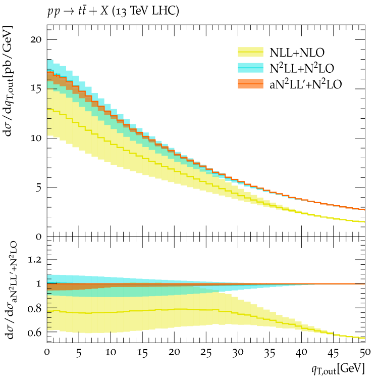
(a) Beam scale $\mu_{b}$ variation

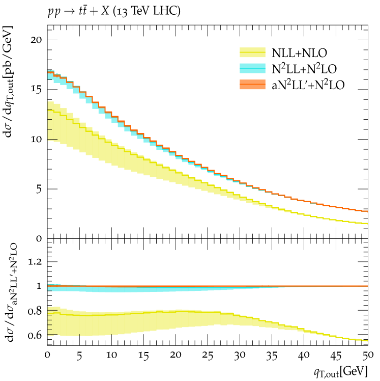
(b) Soft scale $\mu_{s}$ variation

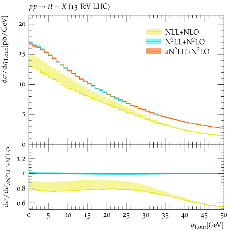
(c) Hard scale $\mu_{h}$ variation

Figure 13: Dependence on the virtuality scales associated with the beam-collinear, soft, and hard sectors of the differential cross section ${\rm d}\sigma_{{t{\bar{t}}}}/{\rm d}q_{\mathrm{T,out}}$.

Fig. 13 details the individual variations of the virtuality scales associated with the beam-collinear, soft, and hard sectors, $\mu_{b}$, $\mu_{s}$, and $\mu_{h}$, respectively. They arise from the renormalisation or subtraction of the virtuality divergences in each regime. As demonstrated in [98], the beam scale $\mu_{b}$ is associated with both the QCD factorisation and the hard-soft-collinear decomposition, such that any variations of $\mu_{b}$ value will induce perturbative corrections from both the solutions of the DGLAP equation [217, 218, 219, 220] and the RGE in Eqs. (3.8)-(3.9). Therefore, as observed in Fig. 13, a variation of the beam scale $\mu_{b}$ generates a larger theoretical uncertainty than a variation of the soft or hard scales, that are only governed by their respective RGEs only, as illustrated in Eq. (3.2) and Eq. (3.11). It is interesting to note that the default choices for $\mu_{s}$ and $\mu_{h}$ produce results that lie on one edge of their respective uncertainty interval, see Fig. 13(b) and Fig. 13(c). This is particularly noticable at NLL. This phenomenon can be interpreted through the evolution kernel in Eq. (3.2), more explicitly,

$$\ln\bigg{[}\frac{\mathcal{D}^{\mathrm{res}}_{[\kappa]}(b_{\mathrm{T}},M_{t{\bar{t}}},\mu_{h},\mu^{\mathrm{def}}_{b},\mu^{\mathrm{def}}_{s},\nu^{\mathrm{def}}_{b},\nu^{\mathrm{def}}_{s})}{\mathcal{D}^{\mathrm{res}}_{[\kappa]}(b_{\mathrm{T}},M_{t{\bar{t}}},\mu^{\mathrm{def}}_{h},\mu^{\mathrm{def}}_{b},\mu^{\mathrm{def}}_{s},\nu^{\mathrm{def}}_{b},\nu^{\mathrm{def}}_{s})}\bigg{]}\Bigg{|}_{\mathrm{NLL}}\, =\,C_{[\kappa]}\Gamma^{(0)}_{\mathrm{cusp}}\frac{\alpha_{s}(M_{t{\bar{t}}})}{4\pi}\frac{1}{2}\ln^{2}\left[\frac{\mu^{2}_{h}}{(\mu^{\mathrm{def}}_{h})^{2}}\right]+\dots\,,$$ (C.1)

$$\ln\bigg{[}\frac{\mathcal{D}^{\mathrm{res}}_{[\kappa]}(b_{\mathrm{T}},M_{t{\bar{t}}},{\mu}^{\mathrm{def}}_{h},\mu^{\mathrm{def}}_{b},\mu_{s},\nu^{\mathrm{def}}_{b},\nu^{\mathrm{def}}_{s})}{\mathcal{D}^{\mathrm{res}}_{[\kappa]}(b_{\mathrm{T}},M_{t{\bar{t}}},\mu^{\mathrm{def}}_{h},\mu^{\mathrm{def}}_{b},\mu^{\mathrm{def}}_{s},\nu^{\mathrm{def}}_{b},\nu^{\mathrm{def}}_{s})}\bigg{]}\Bigg{|}_{\mathrm{NLL}}\, =\,-C_{[\kappa]}\Gamma^{(0)}_{\mathrm{cusp}}\frac{\alpha_{s}(M_{t{\bar{t}}})}{4\pi}\frac{1}{2}\ln^{2}\left[\frac{\mu^{2}_{s}}{(\mu^{\mathrm{def}}_{s})^{2}}\right]+\dots\,,$$ (C.2)

wherein the perturbative expansion of the cusp dimension is given by

$$\Gamma_{\mathrm{cusp}}=\sum_{k=0}^{\infty}\,\Gamma_{\mathrm{cusp}}^{(k)}\,\left(\frac{\alpha_{s}}{4\pi}\right)^{k}\,.$$ (C.3)

In Eqs. (C.1)-(C.2), we only present the leading contributions from the cusp dimension, which dictates the scale dependences at NLL. We observe that at NLL, the default choice of the hard (soft) scale is situated close to the saddle point of the evolution function $\mathcal{D}^{\mathrm{res}}_{[\kappa]}$, such that any changes in the scale will only enhance (reduce) the cross section, prompting the behaviour displayed in Fig. 13(b) and Fig. 13(c). Further increasing the logarithmic accuracy may bring in the fixed order contributions counterbalancing the alternations of $\mathcal{D}^{\mathrm{res}}_{[\kappa]}$. In particular, as for the results at aN²LL^′+N²LO, the inclining trends of the default curves are nearly reversed in comparison to those at lower accuracies.

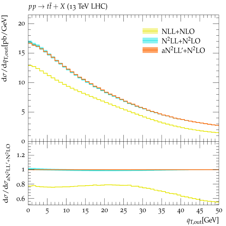
(a) Beam scale $\nu_{b}$ variation

(b) Soft scale $\nu_{s}$ variation

Figure 14: Dependence on the rapidity scales associated with the beam-collinear and soft sectors of the differential cross section ${\rm d}\sigma_{{t{\bar{t}}}}/{\rm d}q_{\mathrm{T,out}}$.

Fig. 14 illustrates the variations induced by scales introduced by regulating the rapidity divergences, $\nu_{b}$ and $\nu_{s}$, respectively. Differing from the converging behaviour in Fig. 13, the theoretical uncertainty here grows from NLL to N²LL. As exhibited in Tab. 1, NLL curves only comprise tree-level fixed order functions and thus the $\nu_{s}$ and $\nu_{b}$ dependences are entirely determined by Eq. (3.2), or, more specifically, the rapidity anomalous dimension $\gamma_{r}$ in Eq. (3.10). However, as presented in [98], $\gamma_{r}$ vanishes in the exponential regularisation prescription at LO. Subsequently, there is no rapidity scale dependence at NLL, as observed in Fig. 13, and the first non-trivial variation induced by $\nu_{s}$ and $\nu_{b}$ occurs at N²LL. Confronting N²LL+N²LO and aN²LL^′+N²LO shows that the manifestly convergent behaviour is also found for the rapidity scale depedences.

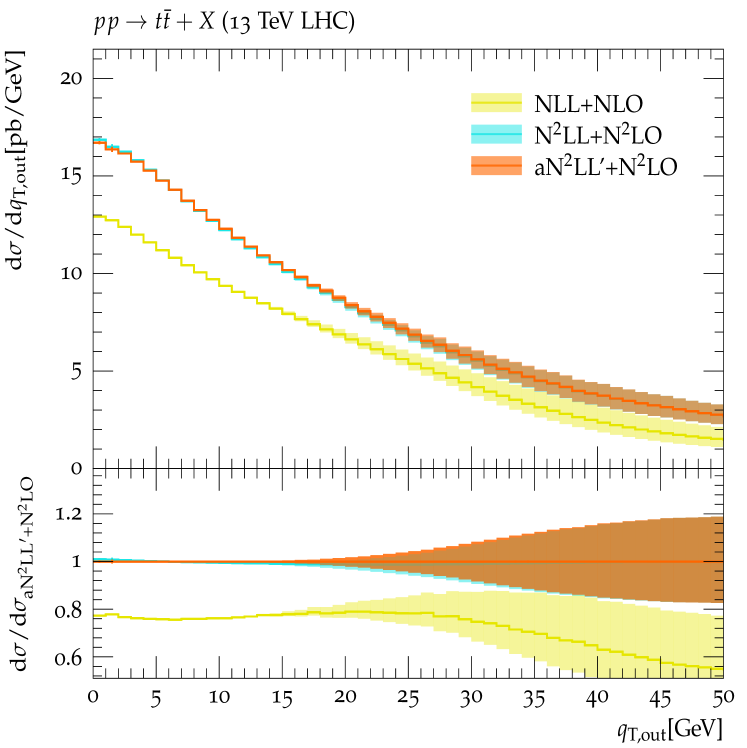
(a) FO scale $\mu_{\mathrm{f.o.}}$ variation

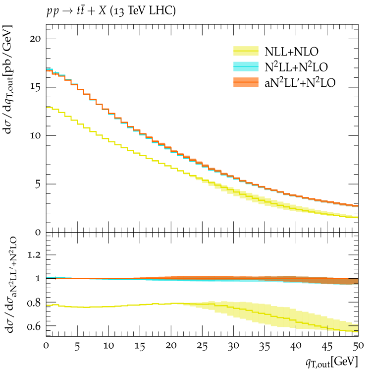
(b) Focal point $c_{m}$ and the transition radius $r_{m}$ variation

Figure 15: Dependence on the fixed-order scale and the matching parameters of the differential cross section ${\rm d}\sigma_{{t{\bar{t}}}}/{\rm d}q_{\mathrm{T,out}}$.

At last, we present the variations of the auxiliary inputs pertinent to the matching procedure, such as the fixed-order scale $\mu_{\mathrm{f.o.}}$ and the shape parameters $\{c_{m},r_{m}\}$ in the transition function. In Fig. 15(a), the $\mu_{\mathrm{f.o.}}$ variation has been assessed. It is seen that the theoretical uncertainties in the asymptotic regime are highly suppressed due to the excellent agreement between QCD and EFT outputs, as demonstrated in Figs. 5-7, but experience continuous growth with the increase in $q_{\mathrm{T},\mathrm{out}}$, as a result of the manifesting power corrections, until the stabilising resummation is switched off and the pure fixed-order behaviour is recovered. The sensitivity of the $q_{\mathrm{T},\mathrm{out}}$ spectrum on the matching transition function parameters $\{c_{m},r_{m}\}$ is illustrated in Fig. 15(b). It, in essence, reflects both the size of the higher power corrections and fixed-order corrections. As expected, the reduction in error bands is discovered along with the improvements on the logarithmic and fixed-order precisions.

References

• [1] ATLAS collaboration, Measurement of the $t\bar{t}$ production cross-section using dilepton events in $pp$ collisions at $\sqrt{s}=5.02$ TeV with the ATLAS detector.
• [2] ATLAS collaboration, Measurement of the $t\bar{t}$ production cross-section in $pp$ collisions at $\sqrt{s}=5.02$ TeV with the ATLAS detector, arXiv:2207.01354 [hep-ex].
• [3] A. M. Sirunyan et al., CMS collaboration, Measurement of the inclusive $\mathrm{t}\overline{\mathrm{t}}$ cross section in pp collisions at $\sqrt{s}=5.02$ TeV using final states with at least one charged lepton, JHEP 03 (2018), 115, [arXiv:1711.03143 [hep-ex]].
• [4] A. Tumasyan et al., CMS collaboration, Measurement of the inclusive $\mathrm{t}\overline{\mathrm{t}}$ production cross section in proton-proton collisions at $\sqrt{s}$ = 5.02 TeV, JHEP 04 (2022), 144, [arXiv:2112.09114 [hep-ex]].
• [5] S. Chatrchyan et al., CMS collaboration, Measurement of the $t\bar{t}$ Production Cross Section in the All-Jet Final State in pp Collisions at $\sqrt{s}$ = 7 TeV, JHEP 05 (2013), 065, [arXiv:1302.0508 [hep-ex]].
• [6] V. Khachatryan et al., CMS collaboration, Measurement of the t-tbar production cross section in the e-mu channel in proton-proton collisions at sqrt(s) = 7 and 8 TeV, JHEP 08 (2016), 029, [arXiv:1603.02303 [hep-ex]].
• [7] ATLAS, CMS collaboration, Combination of inclusive top-quark pair production cross-section measurements using ATLAS and CMS data at $\sqrt{s}=7$ and 8 TeV, arXiv:2205.13830 [hep-ex].
• [8] V. Khachatryan et al., CMS collaboration, Measurement of the $\mathrm{t}\overline{{\mathrm{t}}}$ production cross section in the all-jets final state in pp collisions at $\sqrt{s}=8$TeV, Eur. Phys. J. C 76 (2016), no. 3, 128, [arXiv:1509.06076 [hep-ex]].
• [9] V. Khachatryan et al., CMS collaboration, Measurements of the $\mathrm{t}\overline{\mathrm{t}}$ production cross section in lepton+jets final states in pp collisions at 8  TeV and ratio of 8 to 7  TeV cross sections, Eur. Phys. J. C 77 (2017), no. 1, 15, [arXiv:1602.09024 [hep-ex]].
• [10] G. Aad et al., ATLAS collaboration, Measurement of the $t\bar{t}$ production cross-section and lepton differential distributions in $e\mu$ dilepton events from $pp$ collisions at $\sqrt{s}=13\,\text{TeV}$ with the ATLAS detector, Eur. Phys. J. C 80 (2020), no. 6, 528, [arXiv:1910.08819 [hep-ex]].
• [11] G. Aad et al., ATLAS collaboration, Measurement of the $t\bar{t}$ production cross-section in the lepton+jets channel at $\sqrt{s}=13$ TeV with the ATLAS experiment, Phys. Lett. B 810 (2020), 135797, [arXiv:2006.13076 [hep-ex]].
• [12] G. Aad et al., ATLAS collaboration, Measurements of top-quark pair single- and double-differential cross-sections in the all-hadronic channel in $pp$ collisions at $\sqrt{s}=13~{}\textrm{TeV}$ using the ATLAS detector, JHEP 01 (2021), 033, [arXiv:2006.09274 [hep-ex]].
• [13] A. M. Sirunyan et al., CMS collaboration, Measurement of the top quark pair production cross section in dilepton final states containing one $\tau$ lepton in pp collisions at $\sqrt{s}=$ 13 TeV, JHEP 02 (2020), 191, [arXiv:1911.13204 [hep-ex]].
• [14] CMS collaboration, Measurement of the ${\rm t}{\rm\bar{t}}$ production cross section at 13 TeV in the all-jets final state.
• [15] A. M. Sirunyan et al., CMS collaboration, Measurement of the $\mathrm{t}\overline{\mathrm{t}}$ production cross section, the top quark mass, and the strong coupling constant using dilepton events in pp collisions at $\sqrt{s}=$ 13 TeV, Eur. Phys. J. C 79 (2019), no. 5, 368, [arXiv:1812.10505 [hep-ex]].
• [16] A. Tumasyan et al., CMS collaboration, Measurement of differential $t\bar{t}$ production cross sections in the full kinematic range using lepton+jets events from proton-proton collisions at $\sqrt{s}$ = 13  TeV, Phys. Rev. D 104 (2021), no. 9, 092013, [arXiv:2108.02803 [hep-ex]].
• [17] CMS collaboration, First measurement of the top quark pair production cross section in proton-proton collisions at $\sqrt{s}=13.6\,\mathrm{TeV}$.
• [18] A. M. Sirunyan et al., CMS collaboration, Measurement of $\mathrm{t\bar{t}}$ normalised multi-differential cross sections in pp collisions at $\sqrt{s}=13$ TeV, and simultaneous determination of the strong coupling strength, top quark pole mass, and parton distribution functions, Eur. Phys. J. C 80 (2020), no. 7, 658, [arXiv:1904.05237 [hep-ex]].
• [19] G. Aad et al., ATLAS collaboration, Measurements of differential cross-sections in top-quark pair events with a high transverse momentum top quark and limits on beyond the Standard Model contributions to top-quark pair production with the ATLAS detector at $\sqrt{s}$ = 13 TeV, JHEP 06 (2022), 063, [arXiv:2202.12134 [hep-ex]].
• [20] A. M. Sirunyan et al., CMS collaboration, Measurement of differential $\mathrm{t\bar{t}}$ production cross sections using top quarks at large transverse momenta in $pp$ collisions at $\sqrt{s}=$ 13 TeV, Phys. Rev. D 103 (2021), no. 5, 052008, [arXiv:2008.07860 [hep-ex]].
• [21] CMS collaboration, Measurement of differential cross sections for the production of top quark pairs and of additional jets in pp collisions at $\sqrt{s}=13~{}\mathrm{TeV}$.
• [22] P. Nason, S. Dawson and R. K. Ellis, The Total Cross-Section for the Production of Heavy Quarks in Hadronic Collisions, Nucl. Phys. B 303 (1988), 607–633.
• [23] W. Beenakker, H. Kuijf, W. L. van Neerven and J. Smith, QCD Corrections to Heavy Quark Production in p anti-p Collisions, Phys. Rev. D 40 (1989), 54–82.
• [24] W. Beenakker, W. L. van Neerven, R. Meng, G. A. Schuler and J. Smith, QCD corrections to heavy quark production in hadron hadron collisions, Nucl. Phys. B 351 (1991), 507–560.
• [25] M. L. Mangano, P. Nason and G. Ridolfi, Heavy quark correlations in hadron collisions at next-to-leading order, Nucl. Phys. B 373 (1992), 295–345.
• [26] M. Czakon, P. Fiedler and A. Mitov, Total Top-Quark Pair-Production Cross Section at Hadron Colliders Through $O(\alpha^{4}_{S})$, Phys. Rev. Lett. 110 (2013), 252004, [arXiv:1303.6254 [hep-ph]].
• [27] M. Czakon, D. Heymes and A. Mitov, High-precision differential predictions for top-quark pairs at the LHC, Phys. Rev. Lett. 116 (2016), no. 8, 082003, [arXiv:1511.00549 [hep-ph]].
• [28] M. Czakon, P. Fiedler, D. Heymes and A. Mitov, NNLO QCD predictions for fully-differential top-quark pair production at the Tevatron, JHEP 05 (2016), 034, [arXiv:1601.05375 [hep-ph]].
• [29] M. Czakon, D. Heymes and A. Mitov, fastNLO tables for NNLO top-quark pair differential distributions, arXiv:1704.08551 [hep-ph].
• [30] M. Czakon, D. Heymes, A. Mitov, D. Pagani, I. Tsinikos and M. Zaro, Top-pair production at the LHC through NNLO QCD and NLO EW, JHEP 10 (2017), 186, [arXiv:1705.04105 [hep-ph]].
• [31] S. Catani, S. Devoto, M. Grazzini, S. Kallweit, J. Mazzitelli and H. Sargsyan, Top-quark pair hadroproduction at next-to-next-to-leading order in QCD, Phys. Rev. D 99 (2019), no. 5, 051501, [arXiv:1901.04005 [hep-ph]].
• [32] S. Catani, S. Devoto, M. Grazzini, S. Kallweit and J. Mazzitelli, Top-quark pair hadroproduction at NNLO: differential predictions with the $\overline{MS}$ mass, JHEP 08 (2020), no. 08, 027, [arXiv:2005.00557 [hep-ph]].
• [33] J. Gao, C. S. Li and H. X. Zhu, Top Quark Decay at Next-to-Next-to Leading Order in QCD, Phys. Rev. Lett. 110 (2013), no. 4, 042001, [arXiv:1210.2808 [hep-ph]].
• [34] M. Brucherseifer, F. Caola and K. Melnikov, $\mathcal{O}(\alpha_{s}^{2})$ corrections to fully-differential top quark decays, JHEP 04 (2013), 059, [arXiv:1301.7133 [hep-ph]].
• [35] S. Catani, S. Devoto, M. Grazzini, S. Kallweit and J. Mazzitelli, Top-quark pair production at the LHC: Fully differential QCD predictions at NNLO, JHEP 07 (2019), 100, [arXiv:1906.06535 [hep-ph]].
• [36] A. Behring, M. Czakon, A. Mitov, A. S. Papanastasiou and R. Poncelet, Higher order corrections to spin correlations in top quark pair production at the LHC, Phys. Rev. Lett. 123 (2019), no. 8, 082001, [arXiv:1901.05407 [hep-ph]].
• [37] M. Czakon, A. Mitov and R. Poncelet, NNLO QCD corrections to leptonic observables in top-quark pair production and decay, JHEP 05 (2021), 212, [arXiv:2008.11133 [hep-ph]].
• [38] W. Bernreuther and Z.-G. Si, Distributions and correlations for top quark pair production and decay at the Tevatron and LHC., Nucl. Phys. B 837 (2010), 90–121, [arXiv:1003.3926 [hep-ph]].
• [39] J. H. Kuhn, A. Scharf and P. Uwer, Electroweak effects in top-quark pair production at hadron colliders, Eur. Phys. J. C 51 (2007), 37–53, [hep-ph/0610335].
• [40] W. Bernreuther, M. Fuecker and Z.-G. Si, Weak interaction corrections to hadronic top quark pair production, Phys. Rev. D 74 (2006), 113005, [hep-ph/0610334].
• [41] J. H. Kühn, A. Scharf and P. Uwer, Weak Interactions in Top-Quark Pair Production at Hadron Colliders: An Update, Phys. Rev. D 91 (2015), no. 1, 014020, [arXiv:1305.5773 [hep-ph]].
• [42] W. Hollik and D. Pagani, The electroweak contribution to the top quark forward-backward asymmetry at the Tevatron, Phys. Rev. D 84 (2011), 093003, [arXiv:1107.2606 [hep-ph]].
• [43] D. Pagani, I. Tsinikos and M. Zaro, The impact of the photon PDF and electroweak corrections on $t\bar{t}$ distributions, Eur. Phys. J. C 76 (2016), no. 9, 479, [arXiv:1606.01915 [hep-ph]].
• [44] C. Gütschow, J. M. Lindert and M. Schönherr, Multi-jet merged top-pair production including electroweak corrections, Eur. Phys. J. C 78 (2018), no. 4, 317, [arXiv:1803.00950 [hep-ph]].
• [45] A. Denner and M. Pellen, NLO electroweak corrections to off-shell top-antitop production with leptonic decays at the LHC, JHEP 08 (2016), 155, [arXiv:1607.05571 [hep-ph]].
• [46] N. Kidonakis, NNNLO soft-gluon corrections for the top-quark $p_{T}$ and rapidity distributions, Phys. Rev. D 91 (2015), no. 3, 031501, [arXiv:1411.2633 [hep-ph]].
• [47] N. Kidonakis, Next-to-next-to-leading soft-gluon corrections for the top quark cross section and transverse momentum distribution, Phys. Rev. D 82 (2010), 114030, [arXiv:1009.4935 [hep-ph]].
• [48] N. Kidonakis, Two-loop soft anomalous dimensions and NNLL resummation for heavy quark production, Phys. Rev. Lett. 102 (2009), 232003, [arXiv:0903.2561 [hep-ph]].
• [49] N. Kidonakis, NNNLO soft-gluon corrections for the top-antitop pair production cross section, Phys. Rev. D 90 (2014), no. 1, 014006, [arXiv:1405.7046 [hep-ph]].
• [50] N. Kidonakis, Top-quark double-differential distributions at approximate N3LO, Phys. Rev. D 101 (2020), no. 7, 074006, [arXiv:1912.10362 [hep-ph]].
• [51] V. Ahrens, A. Ferroglia, M. Neubert, B. D. Pecjak and L. L. Yang, Renormalization-Group Improved Predictions for Top-Quark Pair Production at Hadron Colliders, JHEP 09 (2010), 097, [arXiv:1003.5827 [hep-ph]].
• [52] A. Ferroglia, B. D. Pecjak and L. L. Yang, Soft-gluon resummation for boosted top-quark production at hadron colliders, Phys. Rev. D 86 (2012), 034010, [arXiv:1205.3662 [hep-ph]].
• [53] A. Ferroglia, S. Marzani, B. D. Pecjak and L. L. Yang, Boosted top production: factorization and resummation for single-particle inclusive distributions, JHEP 01 (2014), 028, [arXiv:1310.3836 [hep-ph]].
• [54] B. D. Pecjak, D. J. Scott, X. Wang and L. L. Yang, Resummed differential cross sections for top-quark pairs at the LHC, Phys. Rev. Lett. 116 (2016), no. 20, 202001, [arXiv:1601.07020 [hep-ph]].
• [55] M. Czakon, A. Ferroglia, D. Heymes, A. Mitov, B. D. Pecjak, D. J. Scott, X. Wang and L. L. Yang, Resummation for (boosted) top-quark pair production at NNLO+NNLL’ in QCD, JHEP 05 (2018), 149, [arXiv:1803.07623 [hep-ph]].
• [56] P. Hinderer, F. Ringer, G. F. Sterman and W. Vogelsang, Toward NNLL Threshold Resummation for Hadron Pair Production in Hadronic Collisions, Phys. Rev. D 91 (2015), no. 1, 014016, [arXiv:1411.3149 [hep-ph]].
• [57] M. Beneke, M. Czakon, P. Falgari, A. Mitov and C. Schwinn, Threshold expansion of the $gg(q\bar{q})$ $\to\overline{QQ}+X$ cross section at $O(\alpha^{4}_{s})$, Phys. Lett. B 690 (2010), 483–490, [arXiv:0911.5166 [hep-ph]], [Erratum: Phys.Lett.B 778, 464–464 (2018)].
• [58] M. Beneke, P. Falgari and C. Schwinn, Threshold resummation for pair production of coloured heavy (s)particles at hadron colliders, Nucl. Phys. B 842 (2011), 414–474, [arXiv:1007.5414 [hep-ph]].
• [59] M. Beneke, P. Falgari, S. Klein and C. Schwinn, Hadronic top-quark pair production with NNLL threshold resummation, Nucl. Phys. B 855 (2012), 695–741, [arXiv:1109.1536 [hep-ph]].
• [60] M. Cacciari, M. Czakon, M. Mangano, A. Mitov and P. Nason, Top-pair production at hadron colliders with next-to-next-to-leading logarithmic soft-gluon resummation, Phys. Lett. B 710 (2012), 612–622, [arXiv:1111.5869 [hep-ph]].
• [61] J. Piclum and C. Schwinn, Soft-gluon and Coulomb corrections to hadronic top-quark pair production beyond NNLO, JHEP 03 (2018), 164, [arXiv:1801.05788 [hep-ph]].
• [62] W.-L. Ju, G. Wang, X. Wang, X. Xu, Y. Xu and L. L. Yang, Top quark pair production near threshold: single/double distributions and mass determination, JHEP 06 (2020), 158, [arXiv:2004.03088 [hep-ph]].
• [63] W.-L. Ju, G. Wang, X. Wang, X. Xu, Y. Xu and L. L. Yang, Invariant-mass distribution of top-quark pairs and top-quark mass determination, Chin. Phys. C 44 (2020), no. 9, 091001, [arXiv:1908.02179 [hep-ph]].
• [64] H. X. Zhu, C. S. Li, H. T. Li, D. Y. Shao and L. L. Yang, Transverse-momentum resummation for top-quark pairs at hadron colliders, Phys. Rev. Lett. 110 (2013), no. 8, 082001, [arXiv:1208.5774 [hep-ph]].
• [65] H. T. Li, C. S. Li, D. Y. Shao, L. L. Yang and H. X. Zhu, Top quark pair production at small transverse momentum in hadronic collisions, Phys. Rev. D 88 (2013), 074004, [arXiv:1307.2464 [hep-ph]].
• [66] S. Catani, M. Grazzini and A. Torre, Transverse-momentum resummation for heavy-quark hadroproduction, Nucl. Phys. B 890 (2014), 518–538, [arXiv:1408.4564 [hep-ph]].
• [67] S. Catani, M. Grazzini and H. Sargsyan, Azimuthal asymmetries in QCD hard scattering: infrared safe but divergent, JHEP 06 (2017), 017, [arXiv:1703.08468 [hep-ph]].
• [68] S. Catani, M. Grazzini and H. Sargsyan, Transverse-momentum resummation for top-quark pair production at the LHC, JHEP 11 (2018), 061, [arXiv:1806.01601 [hep-ph]].
• [69] S. Alioli, A. Broggio and M. A. Lim, Zero-jettiness resummation for top-quark pair production at the LHC, JHEP 01 (2022), 066, [arXiv:2111.03632 [hep-ph]].
• [70] J. Mazzitelli, P. F. Monni, P. Nason, E. Re, M. Wiesemann and G. Zanderighi, Next-to-Next-to-Leading Order Event Generation for Top-Quark Pair Production, Phys. Rev. Lett. 127 (2021), no. 6, 062001, [arXiv:2012.14267 [hep-ph]].
• [71] J. Mazzitelli, P. F. Monni, P. Nason, E. Re, M. Wiesemann and G. Zanderighi, Top-pair production at the LHC with MINNLOPS, JHEP 04 (2022), 079, [arXiv:2112.12135 [hep-ph]].
• [72] P. M. Nadolsky, C. Balazs, E. L. Berger and C. P. Yuan, Gluon-gluon contributions to the production of continuum diphoton pairs at hadron colliders, Phys. Rev. D 76 (2007), 013008, [hep-ph/0702003].
• [73] S. Catani and M. Grazzini, QCD transverse-momentum resummation in gluon fusion processes, Nucl. Phys. B 845 (2011), 297–323, [arXiv:1011.3918 [hep-ph]].
• [74] J. C. Collins, INTRINSIC TRANSVERSE MOMENTUM. 1. NONGAUGE THEORIES, Phys. Rev. D 21 (1980), 2962.
• [75] G. F. Sterman, Mass Divergences in Annihilation Processes. 1. Origin and Nature of Divergences in Cut Vacuum Polarization Diagrams, Phys. Rev. D 17 (1978), 2773.
• [76] L. D. Landau, On analytic properties of vertex parts in quantum field theory, Nucl. Phys. 13 (1959), no. 1, 181–192.
• [77] S. Coleman and R. E. Norton, Singularities in the physical region, Nuovo Cim. 38 (1965), 438–442.
• [78] M. Beneke and V. A. Smirnov, Asymptotic expansion of Feynman integrals near threshold, Nucl. Phys. B 522 (1998), 321–344, [hep-ph/9711391].
• [79] V. A. Smirnov, Applied asymptotic expansions in momenta and masses, Springer Tracts Mod. Phys. 177 (2002), 1–262.
• [80] V. A. Smirnov, Analytic tools for Feynman integrals, vol. 250, 2012.
• [81] B. Jantzen, Foundation and generalization of the expansion by regions, JHEP 12 (2011), 076, [arXiv:1111.2589 [hep-ph]].
• [82] C. W. Bauer, D. Pirjol and I. W. Stewart, Soft collinear factorization in effective field theory, Phys. Rev. D 65 (2002), 054022, [hep-ph/0109045].
• [83] C. W. Bauer and I. W. Stewart, Invariant operators in collinear effective theory, Phys. Lett. B 516 (2001), 134–142, [hep-ph/0107001].
• [84] C. W. Bauer, S. Fleming, D. Pirjol and I. W. Stewart, An Effective field theory for collinear and soft gluons: Heavy to light decays, Phys. Rev. D 63 (2001), 114020, [hep-ph/0011336].
• [85] C. W. Bauer, S. Fleming and M. E. Luke, Summing Sudakov logarithms in $B\to X_{s}\gamma$in effective field theory., Phys. Rev. D 63 (2000), 014006, [hep-ph/0005275].
• [86] C. W. Bauer, S. Fleming, D. Pirjol, I. Z. Rothstein and I. W. Stewart, Hard scattering factorization from effective field theory, Phys. Rev. D 66 (2002), 014017, [hep-ph/0202088].
• [87] M. Beneke, A. P. Chapovsky, M. Diehl and T. Feldmann, Soft collinear effective theory and heavy to light currents beyond leading power, Nucl. Phys. B 643 (2002), 431–476, [hep-ph/0206152].
• [88] M. Beneke and T. Feldmann, Multipole expanded soft collinear effective theory with nonAbelian gauge symmetry, Phys. Lett. B 553 (2003), 267–276, [hep-ph/0211358].
• [89] C. W. Bauer, D. Pirjol and I. W. Stewart, Factorization and endpoint singularities in heavy to light decays, Phys. Rev. D 67 (2003), 071502, [hep-ph/0211069].
• [90] B. O. Lange and M. Neubert, Factorization and the soft overlap contribution to heavy to light form-factors, Nucl. Phys. B 690 (2004), 249–278, [hep-ph/0311345], [Erratum: Nucl.Phys.B 723, 201–202 (2005)].
• [91] M. Beneke and T. Feldmann, Factorization of heavy to light form-factors in soft collinear effective theory, Nucl. Phys. B 685 (2004), 249–296, [hep-ph/0311335].
• [92] E. Eichten and B. R. Hill, An Effective Field Theory for the Calculation of Matrix Elements Involving Heavy Quarks, Phys. Lett. B 234 (1990), 511–516.
• [93] H. Georgi, An Effective Field Theory for Heavy Quarks at Low-energies, Phys. Lett. B 240 (1990), 447–450.
• [94] B. Grinstein, The Static Quark Effective Theory, Nucl. Phys. B 339 (1990), 253–268.
• [95] M. Neubert, Heavy quark symmetry, Phys. Rept. 245 (1994), 259–396, [hep-ph/9306320].
• [96] J.-y. Chiu, A. Jain, D. Neill and I. Z. Rothstein, The Rapidity Renormalization Group, Phys. Rev. Lett. 108 (2012), 151601, [arXiv:1104.0881 [hep-ph]].
• [97] J.-Y. Chiu, A. Jain, D. Neill and I. Z. Rothstein, A Formalism for the Systematic Treatment of Rapidity Logarithms in Quantum Field Theory, JHEP 05 (2012), 084, [arXiv:1202.0814 [hep-ph]].
• [98] Y. Li, D. Neill and H. X. Zhu, An exponential regulator for rapidity divergences, Nucl. Phys. B 960 (2020), 115193, [arXiv:1604.00392 [hep-ph]].
• [99] Y. Li and H. X. Zhu, Bootstrapping Rapidity Anomalous Dimensions for Transverse-Momentum Resummation, Phys. Rev. Lett. 118 (2017), no. 2, 022004, [arXiv:1604.01404 [hep-ph]].
• [100] J. C. Collins, D. E. Soper and G. F. Sterman, Transverse Momentum Distribution in Drell-Yan Pair and W and Z Boson Production, Nucl. Phys. B 250 (1985), 199–224.
• [101] S. Catani, D. de Florian and M. Grazzini, Universality of nonleading logarithmic contributions in transverse momentum distributions, Nucl. Phys. B 596 (2001), 299–312, [hep-ph/0008184].
• [102] G. Bozzi, S. Catani, D. de Florian and M. Grazzini, Transverse-momentum resummation and the spectrum of the Higgs boson at the LHC, Nucl. Phys. B 737 (2006), 73–120, [hep-ph/0508068].
• [103] G. Bozzi, S. Catani, D. de Florian and M. Grazzini, Higgs boson production at the LHC: Transverse-momentum resummation and rapidity dependence, Nucl. Phys. B 791 (2008), 1–19, [arXiv:0705.3887 [hep-ph]].
• [104] M. A. Ebert and F. J. Tackmann, Resummation of Transverse Momentum Distributions in Distribution Space, JHEP 02 (2017), 110, [arXiv:1611.08610 [hep-ph]].
• [105] P. F. Monni, E. Re and P. Torrielli, Higgs Transverse-Momentum Resummation in Direct Space, Phys. Rev. Lett. 116 (2016), no. 24, 242001, [arXiv:1604.02191 [hep-ph]].
• [106] W. Bizon, P. F. Monni, E. Re, L. Rottoli and P. Torrielli, Momentum-space resummation for transverse observables and the Higgs p at N3LL+NNLO, JHEP 02 (2018), 108, [arXiv:1705.09127 [hep-ph]].
• [107] T. Becher and M. Neubert, Drell-Yan Production at Small $q_{T}$, Transverse Parton Distributions and the Collinear Anomaly, Eur. Phys. J. C 71 (2011), 1665, [arXiv:1007.4005 [hep-ph]].
• [108] M. G. Echevarria, A. Idilbi and I. Scimemi, Factorization Theorem For Drell-Yan At Low $q_{T}$ And Transverse Momentum Distributions On-The-Light-Cone, JHEP 07 (2012), 002, [arXiv:1111.4996 [hep-ph]].
• [109] T. Becher and G. Bell, Analytic Regularization in Soft-Collinear Effective Theory, Phys. Lett. B 713 (2012), 41–46, [arXiv:1112.3907 [hep-ph]].
• [110] J. C. Collins, D. E. Soper and G. F. Sterman, Factorization of Hard Processes in QCD, Adv. Ser. Direct. High Energy Phys. 5 (1989), 1–91, [hep-ph/0409313].
• [111] A. V. Manohar and I. W. Stewart, The Zero-Bin and Mode Factorization in Quantum Field Theory, Phys. Rev. D 76 (2007), 074002, [hep-ph/0605001].
• [112] B. Ananthanarayan, A. Pal, S. Ramanan and R. Sarkar, Unveiling Regions in multi-scale Feynman Integrals using Singularities and Power Geometry, Eur. Phys. J. C 79 (2019), no. 1, 57, [arXiv:1810.06270 [hep-ph]].
• [113] J. Plenter and G. Rodrigo, Asymptotic expansions through the loop-tree duality, Eur. Phys. J. C 81 (2021), no. 4, 320, [arXiv:2005.02119 [hep-ph]].
• [114] G. Heinrich, S. Jahn, S. P. Jones, M. Kerner, F. Langer, V. Magerya, A. Pöldaru, J. Schlenk and E. Villa, Expansion by regions with pySecDec, Comput. Phys. Commun. 273 (2022), 108267, [arXiv:2108.10807 [hep-ph]].
• [115] J. C. Collins and G. F. Sterman, Soft Partons in QCD, Nucl. Phys. B 185 (1981), 172–188.
• [116] J. C. Collins, D. E. Soper and G. F. Sterman, Factorization for Short Distance Hadron - Hadron Scattering, Nucl. Phys. B 261 (1985), 104–142.
• [117] J. C. Collins, Proof of factorization for diffractive hard scattering, Phys. Rev. D 57 (1998), 3051–3056, [hep-ph/9709499], [Erratum: Phys.Rev.D 61, 019902 (2000)].
• [118] J. C. Collins and A. Metz, Universality of soft and collinear factors in hard-scattering factorization, Phys. Rev. Lett. 93 (2004), 252001, [hep-ph/0408249].
• [119] J. R. Gaunt, Glauber Gluons and Multiple Parton Interactions, JHEP 07 (2014), 110, [arXiv:1405.2080 [hep-ph]].
• [120] M. D. Schwartz, K. Yan and H. X. Zhu, Factorization Violation and Scale Invariance, Phys. Rev. D 97 (2018), no. 9, 096017, [arXiv:1801.01138 [hep-ph]].
• [121] S.-J. Chang and S.-K. Ma, Feynman rules and quantum electrodynamics at infinite momentum, Phys. Rev. 180 (1969), 1506–1513.
• [122] G. F. Sterman, Mass Divergences in Annihilation Processes. 2. Cancellation of Divergences in Cut Vacuum Polarization Diagrams, Phys. Rev. D 17 (1978), 2789.
• [123] A. Mitov and G. Sterman, Final state interactions in single- and multi-particle inclusive cross sections for hadronic collisions, Phys. Rev. D 86 (2012), 114038, [arXiv:1209.5798 [hep-ph]].
• [124] I. Z. Rothstein and I. W. Stewart, An Effective Field Theory for Forward Scattering and Factorization Violation, JHEP 08 (2016), 025, [arXiv:1601.04695 [hep-ph]].
• [125] T. C. Rogers and P. J. Mulders, No Generalized TMD-Factorization in Hadro-Production of High Transverse Momentum Hadrons, Phys. Rev. D 81 (2010), 094006, [arXiv:1001.2977 [hep-ph]].
• [126] J. F. Donoghue and D. Wyler, On Regge kinematics in SCET, Phys. Rev. D 81 (2010), 114023, [arXiv:0908.4559 [hep-ph]].
• [127] C. W. Bauer, B. O. Lange and G. Ovanesyan, On Glauber modes in Soft-Collinear Effective Theory, JHEP 07 (2011), 077, [arXiv:1010.1027 [hep-ph]].
• [128] S. Fleming, The role of Glauber exchange in soft collinear effective theory and the Balitsky–Fadin–Kuraev–Lipatov Equation, Phys. Lett. B 735 (2014), 266–271, [arXiv:1404.5672 [hep-ph]].
• [129] I. Moult, S. Raman, G. Ridgway and I. W. Stewart, Anomalous Dimensions from Soft Regge Constants, arXiv:2207.02859 [hep-ph].
• [130] R. Bonciani, S. Catani, M. Grazzini, H. Sargsyan and A. Torre, The $q_{T}$ subtraction method for top quark production at hadron colliders, Eur. Phys. J. C 75 (2015), no. 12, 581, [arXiv:1508.03585 [hep-ph]].
• [131] J. C. Collins and D. E. Soper, Back-To-Back Jets in QCD, Nucl. Phys. B 193 (1981), 381, [Erratum: Nucl.Phys.B 213, 545 (1983)].
• [132] R. J. Hill and M. Neubert, Spectator interactions in soft collinear effective theory, Nucl. Phys. B 657 (2003), 229–256, [hep-ph/0211018].
• [133] M. Beneke, P. Falgari and C. Schwinn, Soft radiation in heavy-particle pair production: All-order colour structure and two-loop anomalous dimension, Nucl. Phys. B 828 (2010), 69–101, [arXiv:0907.1443 [hep-ph]].
• [134] A. Ferroglia, M. Neubert, B. D. Pecjak and L. L. Yang, Two-loop divergences of massive scattering amplitudes in non-abelian gauge theories, JHEP 11 (2009), 062, [arXiv:0908.3676 [hep-ph]].
• [135] S. Actis, A. Denner, L. Hofer, A. Scharf and S. Uccirati, Recursive generation of one-loop amplitudes in the Standard Model, JHEP 04 (2013), 037, [arXiv:1211.6316 [hep-ph]].
• [136] S. Actis, A. Denner, L. Hofer, J.-N. Lang, A. Scharf and S. Uccirati, RECOLA: REcursive Computation of One-Loop Amplitudes, Comput. Phys. Commun. 214 (2017), 140–173, [arXiv:1605.01090 [hep-ph]].
• [137] L. Chen, M. Czakon and R. Poncelet, Polarized double-virtual amplitudes for heavy-quark pair production, JHEP 03 (2018), 085, [arXiv:1712.08075 [hep-ph]].
• [138] S. Di Vita, T. Gehrmann, S. Laporta, P. Mastrolia, A. Primo and U. Schubert, Master integrals for the NNLO virtual corrections to $q\overline{q}\to t\overline{t}$ scattering in QCD: the non-planar graphs, JHEP 06 (2019), 117, [arXiv:1904.10964 [hep-ph]].
• [139] S. Badger, E. Chaubey, H. B. Hartanto and R. Marzucca, Two-loop leading colour QCD helicity amplitudes for top quark pair production in the gluon fusion channel, JHEP 06 (2021), 163, [arXiv:2102.13450 [hep-ph]].
• [140] M. K. Mandal, P. Mastrolia, J. Ronca and W. J. Bobadilla Torres, Two-loop scattering amplitude for heavy-quark pair production through light-quark annihilation in QCD, JHEP 09 (2022), 129, [arXiv:2204.03466 [hep-ph]].
• [141] M.-X. Luo, X. Wang, X. Xu, L. L. Yang, T.-Z. Yang and H. X. Zhu, Transverse Parton Distribution and Fragmentation Functions at NNLO: the Quark Case, JHEP 10 (2019), 083, [arXiv:1908.03831 [hep-ph]].
• [142] M.-X. Luo, T.-Z. Yang, H. X. Zhu and Y. J. Zhu, Transverse Parton Distribution and Fragmentation Functions at NNLO: the Gluon Case, JHEP 01 (2020), 040, [arXiv:1909.13820 [hep-ph]].
• [143] M.-x. Luo, T.-Z. Yang, H. X. Zhu and Y. J. Zhu, Unpolarized quark and gluon TMD PDFs and FFs at N3LO, JHEP 06 (2021), 115, [arXiv:2012.03256 [hep-ph]].
• [144] M.-x. Luo, T.-Z. Yang, H. X. Zhu and Y. J. Zhu, Quark Transverse Parton Distribution at the Next-to-Next-to-Next-to-Leading Order, Phys. Rev. Lett. 124 (2020), no. 9, 092001, [arXiv:1912.05778 [hep-ph]].
• [145] D. Gutierrez-Reyes, S. Leal-Gomez, I. Scimemi and A. Vladimirov, Linearly polarized gluons at next-to-next-to leading order and the Higgs transverse momentum distribution, JHEP 11 (2019), 121, [arXiv:1907.03780 [hep-ph]].
• [146] S. Catani and P. K. Dhani, Collinear functions for QCD resummations, arXiv:2208.05840 [hep-ph].
• [147] R. Angeles-Martinez, M. Czakon and S. Sapeta, NNLO soft function for top quark pair production at small transverse momentum, JHEP 10 (2018), 201, [arXiv:1809.01459 [hep-ph]].
• [148] S. Catani, I. Fabre, M. Grazzini and S. Kallweit, ${t{{\bar{t}}}H}$ production at NNLO: the flavour off-diagonal channels, Eur. Phys. J. C 81 (2021), no. 6, 491, [arXiv:2102.03256 [hep-ph]].
• [149] A. Pineda and J. Soto, Effective field theory for ultrasoft momenta in NRQCD and NRQED, Nucl. Phys. B Proc. Suppl. 64 (1998), 428–432, [hep-ph/9707481].
• [150] N. Brambilla, A. Pineda, J. Soto and A. Vairo, Potential NRQCD: An Effective theory for heavy quarkonium, Nucl. Phys. B 566 (2000), 275, [hep-ph/9907240].
• [151] M. Beneke, Perturbative heavy quark - anti-quark systems, PoS hf8 (1999), 009, [hep-ph/9911490].
• [152] M. Beneke, A. Signer and V. A. Smirnov, Top quark production near threshold and the top quark mass, Phys. Lett. B 454 (1999), 137–146, [hep-ph/9903260].
• [153] W.-L. Ju and L. L. Yang, Resummation of soft and Coulomb corrections for $t\overline{t}h$ production at the LHC, JHEP 06 (2019), 050, [arXiv:1904.08744 [hep-ph]].
• [154] S. Fleming and A. K. Leibovich, The Resummed Photon Spectrum in Radiative Upsilon Decays, Phys. Rev. Lett. 90 (2003), 032001, [hep-ph/0211303].
• [155] S. Fleming and A. K. Leibovich, The Photon Spectrum in Upsilon Decays, Phys. Rev. D 67 (2003), 074035, [hep-ph/0212094].
• [156] T. Becher and G. Bell, The gluon jet function at two-loop order, Phys. Lett. B 695 (2011), 252–258, [arXiv:1008.1936 [hep-ph]].
• [157] P. Banerjee, P. K. Dhani and V. Ravindran, Gluon jet function at three loops in QCD, Phys. Rev. D 98 (2018), no. 9, 094016, [arXiv:1805.02637 [hep-ph]].
• [158] T. Becher and M. Neubert, Toward a NNLO calculation of the anti-B —$>$ X(s) gamma decay rate with a cut on photon energy. II. Two-loop result for the jet function, Phys. Lett. B 637 (2006), 251–259, [hep-ph/0603140].
• [159] R. Brüser, Z. L. Liu and M. Stahlhofen, Three-Loop Quark Jet Function, Phys. Rev. Lett. 121 (2018), no. 7, 072003, [arXiv:1804.09722 [hep-ph]].
• [160] T. Becher, M. Neubert, L. Rothen and D. Y. Shao, Factorization and Resummation for Jet Processes, JHEP 11 (2016), 019, [arXiv:1605.02737 [hep-ph]], [Erratum: JHEP 05, 154 (2017)].
• [161] M. Balsiger, T. Becher and A. Ferroglia, Resummation of non-global logarithms in cross sections with massive particles, JHEP 09 (2020), 029, [arXiv:2006.00014 [hep-ph]].
• [162] S. Catani and M. H. Seymour, A General algorithm for calculating jet cross-sections in NLO QCD, Nucl. Phys. B 485 (1997), 291–419, [hep-ph/9605323], [Erratum: Nucl.Phys.B 510, 503–504 (1998)].
• [163] V. A. Smirnov, Analytical result for dimensionally regularized massless on shell double box, Phys. Lett. B 460 (1999), 397–404, [hep-ph/9905323].
• [164] J. B. Tausk, Nonplanar massless two loop Feynman diagrams with four on-shell legs, Phys. Lett. B 469 (1999), 225–234, [hep-ph/9909506].
• [165] E. Bejdakic, Feynman integrals, hypergeometric functions and nested sums, Other thesis, 10 2009.
• [166] M. Czakon, Automatized analytic continuation of Mellin-Barnes integrals, Comput. Phys. Commun. 175 (2006), 559–571, [hep-ph/0511200].
• [167] M. Czakon, MBasymptotics, https://mbtools.hepforge.org.
• [168] M. Ochman and T. Riemann, MBsums - a Mathematica package for the representation of Mellin-Barnes integrals by multiple sums, Acta Phys. Polon. B 46 (2015), no. 11, 2117, [arXiv:1511.01323 [hep-ph]].
• [169] T. Gleisberg, S. Hoeche, F. Krauss, A. Schalicke, S. Schumann and J.-C. Winter, SHERPA 1. alpha: A Proof of concept version, JHEP 02 (2004), 056, [hep-ph/0311263].
• [170] T. Gleisberg, S. Hoeche, F. Krauss, M. Schonherr, S. Schumann, F. Siegert and J. Winter, Event generation with SHERPA 1.1, JHEP 02 (2009), 007, [arXiv:0811.4622 [hep-ph]].
• [171] E. Bothmann et al., Sherpa collaboration, Event Generation with Sherpa 2.2, SciPost Phys. 7 (2019), no. 3, 034, [arXiv:1905.09127 [hep-ph]].
• [172] A. Ferroglia, M. Neubert, B. D. Pecjak and L. L. Yang, Two-loop divergences of scattering amplitudes with massive partons, Phys. Rev. Lett. 103 (2009), 201601, [arXiv:0907.4791 [hep-ph]].
• [173] S. Moch, J. A. M. Vermaseren and A. Vogt, The Three loop splitting functions in QCD: The Nonsinglet case, Nucl. Phys. B 688 (2004), 101–134, [hep-ph/0403192].
• [174] J. M. Henn, G. P. Korchemsky and B. Mistlberger, The full four-loop cusp anomalous dimension in $\mathcal{N}=4$ super Yang-Mills and QCD, JHEP 04 (2020), 018, [arXiv:1911.10174 [hep-th]].
• [175] A. von Manteuffel, E. Panzer and R. M. Schabinger, Cusp and collinear anomalous dimensions in four-loop QCD from form factors, Phys. Rev. Lett. 124 (2020), no. 16, 162001, [arXiv:2002.04617 [hep-ph]].
• [176] F. Herzog, S. Moch, B. Ruijl, T. Ueda, J. A. M. Vermaseren and A. Vogt, Five-loop contributions to low-N non-singlet anomalous dimensions in QCD, Phys. Lett. B 790 (2019), 436–443, [arXiv:1812.11818 [hep-ph]].
• [177] Z. L. Liu and N. Schalch, Infrared Singularities of Multileg QCD Amplitudes with a Massive Parton at Three Loops, Phys. Rev. Lett. 129 (2022), no. 23, 232001, [arXiv:2207.02864 [hep-ph]].
• [178] A. A. Vladimirov, Correspondence between Soft and Rapidity Anomalous Dimensions, Phys. Rev. Lett. 118 (2017), no. 6, 062001, [arXiv:1610.05791 [hep-ph]].
• [179] M. A. Ebert, B. Mistlberger and G. Vita, Transverse momentum dependent PDFs at N3LO, JHEP 09 (2020), 146, [arXiv:2006.05329 [hep-ph]].
• [180] G. Das, S.-O. Moch and A. Vogt, Soft corrections to inclusive deep-inelastic scattering at four loops and beyond, JHEP 03 (2020), 116, [arXiv:1912.12920 [hep-ph]].
• [181] C. Duhr, B. Mistlberger and G. Vita, Soft integrals and soft anomalous dimensions at N3LO and beyond, JHEP 09 (2022), 155, [arXiv:2205.04493 [hep-ph]].
• [182] C. Duhr, B. Mistlberger and G. Vita, Four-Loop Rapidity Anomalous Dimension and Event Shapes to Fourth Logarithmic Order, Phys. Rev. Lett. 129 (2022), no. 16, 162001, [arXiv:2205.02242 [hep-ph]].
• [183] I. Moult, H. X. Zhu and Y. J. Zhu, The four loop QCD rapidity anomalous dimension, JHEP 08 (2022), 280, [arXiv:2205.02249 [hep-ph]].
• [184] D. Neill, I. Z. Rothstein and V. Vaidya, The Higgs Transverse Momentum Distribution at NNLL and its Theoretical Errors, JHEP 12 (2015), 097, [arXiv:1503.00005 [hep-ph]].
• [185] D. Kang, C. Lee and V. Vaidya, A fast and accurate method for perturbative resummation of transverse momentum-dependent observables, JHEP 04 (2018), 149, [arXiv:1710.00078 [hep-ph]].
• [186] A. J. Buras, M. Jamin, M. E. Lautenbacher and P. H. Weisz, Effective Hamiltonians for $\Delta S=1$ and $\Delta B=1$ nonleptonic decays beyond the leading logarithmic approximation, Nucl. Phys. B 370 (1992), 69–104, [Addendum: Nucl.Phys.B 375, 501 (1992)].
• [187] G. Buchalla, A. J. Buras and M. E. Lautenbacher, Weak decays beyond leading logarithms, Rev. Mod. Phys. 68 (1996), 1125–1144, [hep-ph/9512380].
• [188] A. Banfi, P. F. Monni, G. P. Salam and G. Zanderighi, Higgs and Z-boson production with a jet veto, Phys. Rev. Lett. 109 (2012), 202001, [arXiv:1206.4998 [hep-ph]].
• [189] A. Banfi, G. P. Salam and G. Zanderighi, NLL+NNLO predictions for jet-veto efficiencies in Higgs-boson and Drell-Yan production, JHEP 06 (2012), 159, [arXiv:1203.5773 [hep-ph]].
• [190] W. Bizoń, X. Chen, A. Gehrmann-De Ridder, T. Gehrmann, N. Glover, A. Huss, P. F. Monni, E. Re, L. Rottoli and P. Torrielli, Fiducial distributions in Higgs and Drell-Yan production at N3LL+NNLO, JHEP 12 (2018), 132, [arXiv:1805.05916 [hep-ph]].
• [191] R. L. Workman et al., Particle Data Group collaboration, Review of Particle Physics, PTEP 2022 (2022), 083C01.
• [192] J. Ablinger, J. Blümlein, M. Round and C. Schneider, Numerical Implementation of Harmonic Polylogarithms to Weight w = 8, Comput. Phys. Commun. 240 (2019), 189–201, [arXiv:1809.07084 [hep-ph]].
• [193] R. D. Ball et al., NNPDF collaboration, Parton distributions from high-precision collider data, Eur. Phys. J. C 77 (2017), no. 10, 663, [arXiv:1706.00428 [hep-ph]].
• [194] A. Buckley, J. Ferrando, S. Lloyd, K. Nordström, B. Page, M. Rüfenacht, M. Schönherr and G. Watt, LHAPDF6: parton density access in the LHC precision era, Eur. Phys. J. C 75 (2015), 132, [arXiv:1412.7420 [hep-ph]].
• [195] E. Bothmann, A. Buckley, I. A. Christidi, C. Gütschow, S. Höche, M. Knobbe, T. Martin and M. Schönherr, Accelerating LHC event generation with simplified pilot runs and fast PDFs, arXiv:2209.00843 [hep-ph].
• [196] T. Becher, M. Neubert and B. D. Pecjak, Factorization and Momentum-Space Resummation in Deep-Inelastic Scattering, JHEP 01 (2007), 076, [hep-ph/0607228].
• [197] T. Hahn, Routines for the diagonalization of complex matrices, physics/0607103.
• [198] A. Buckley, J. Butterworth, D. Grellscheid, H. Hoeth, L. Lonnblad, J. Monk, H. Schulz and F. Siegert, Rivet user manual, Comput. Phys. Commun. 184 (2013), 2803–2819, [arXiv:1003.0694 [hep-ph]].
• [199] C. Bierlich et al., Robust Independent Validation of Experiment and Theory: Rivet version 3, SciPost Phys. 8 (2020), 026, [arXiv:1912.05451 [hep-ph]].
• [200] F. Krauss, R. Kuhn and G. Soff, AMEGIC++ 1.0: A Matrix element generator in C++, JHEP 02 (2002), 044, [hep-ph/0109036].
• [201] S. Catani, S. Dittmaier, M. H. Seymour and Z. Trocsanyi, The Dipole formalism for next-to-leading order QCD calculations with massive partons, Nucl. Phys. B 627 (2002), 189–265, [hep-ph/0201036].
• [202] T. Gleisberg and F. Krauss, Automating dipole subtraction for QCD NLO calculations, Eur. Phys. J. C 53 (2008), 501–523, [arXiv:0709.2881 [hep-ph]].
• [203] M. Schönherr, An automated subtraction of NLO EW infrared divergences, Eur. Phys. J. C 78 (2018), no. 2, 119, [arXiv:1712.07975 [hep-ph]].
• [204] W.-L. Ju and M. Schönherr, The qT and $\Delta$ $\phi$ spectra in W and Z production at the LHC at N3LL’+N2LO, JHEP 10 (2021), 088, [arXiv:2106.11260 [hep-ph]].
• [205] A. Gao, J. K. L. Michel, I. W. Stewart and Z. Sun, A Better Angle on Hadron Transverse Momentum Distributions at the EIC, arXiv:2209.11211 [hep-ph].
• [206] Y.-T. Chien, D. Y. Shao and B. Wu, Resummation of Boson-Jet Correlation at Hadron Colliders, JHEP 11 (2019), 025, [arXiv:1905.01335 [hep-ph]].
• [207] R. F. del Castillo, M. G. Echevarria, Y. Makris and I. Scimemi, Transverse momentum dependent distributions in dijet and heavy hadron pair production at EIC, JHEP 03 (2022), 047, [arXiv:2111.03703 [hep-ph]].
• [208] X.-B. Tong, B.-W. Xiao and Y.-Y. Zhang, Harmonics of Parton Saturation in Lepton-Jet Correlations at the EIC, arXiv:2211.01647 [hep-ph].
• [209] D. Y. Shao, C. Zhang, J. Zhou and Y. Zhou, Azimuthal asymmetries of muon pair production in ultraperipheral heavy ion collisions, arXiv:2212.05775 [hep-ph].
• [210] L. Chen, G.-Y. Qin, L. Wang, S.-Y. Wei, B.-W. Xiao, H.-Z. Zhang and Y.-Q. Zhang, Study of Isolated-photon and Jet Momentum Imbalance in $pp$ and $PbPb$ collisions, Nucl. Phys. B 933 (2018), 306–319, [arXiv:1803.10533 [hep-ph]].
• [211] Y.-T. Chien, R. Rahn, S. Schrijnder van Velzen, D. Y. Shao, W. J. Waalewijn and B. Wu, Recoil-free azimuthal angle for precision boson-jet correlation, Phys. Lett. B 815 (2021), 136124, [arXiv:2005.12279 [hep-ph]].
• [212] H. Bouaziz, Y. Delenda and K. Khelifa-Kerfa, Azimuthal decorrelation between a jet and a Z boson at hadron colliders, JHEP 10 (2022), 006, [arXiv:2207.10147 [hep-ph]].
• [213] Y.-T. Chien, R. Rahn, D. Y. Shao, W. J. Waalewijn and B. Wu, Precision boson-jet azimuthal decorrelation at hadron colliders, arXiv:2205.05104 [hep-ph].
• [214] A. Banfi, M. Dasgupta and Y. Delenda, Azimuthal decorrelations between QCD jets at all orders, Phys. Lett. B 665 (2008), 86–91, [arXiv:0804.3786 [hep-ph]].
• [215] C. Zhang, Q.-S. Dai and D. Y. Shao, Azimuthal decorrelation for photon induced dijet production in ultra-peripheral collisions of heavy ions, arXiv:2211.07071 [hep-ph].
• [216] P. A. Baikov, K. G. Chetyrkin and J. H. Kühn, Five-Loop Running of the QCD coupling constant, Phys. Rev. Lett. 118 (2017), no. 8, 082002, [arXiv:1606.08659 [hep-ph]].
• [217] L. N. Lipatov, The parton model and perturbation theory, Yad. Fiz. 20 (1974), 181–198.
• [218] V. N. Gribov and L. N. Lipatov, Deep inelastic e p scattering in perturbation theory, Sov. J. Nucl. Phys. 15 (1972), 438–450.
• [219] G. Altarelli and G. Parisi, Asymptotic Freedom in Parton Language, Nucl. Phys. B 126 (1977), 298–318.
• [220] Y. L. Dokshitzer, Calculation of the Structure Functions for Deep Inelastic Scattering and e+ e- Annihilation by Perturbation Theory in Quantum Chromodynamics., Sov. Phys. JETP 46 (1977), 641–653.