Abstract

In this paper, we compare the saturation time scales for complexity, linear entropy and entanglement negativity for two open quantum systems. Our first model is a coupled harmonic oscillator, where we treat one of the oscillators as the bath. The second one is a type of Caldeira Leggett model, where we consider a one-dimensional free scalar field as the bath. Using these open quantum systems, we discovered that both the complexity of purification and the complexity from operator state mapping is always saturated for a completely mixed state. More explicitly, the saturation time scale for both types of complexity is smaller than the saturation time scale for linear entropy. On top of this, we found that the saturation time scale for linear entropy and entanglement negativity is of the same order for the Caldeira Leggett model.

1 Introduction

Understanding the transition of quantum to classical behaviour is an important problem in many branches of physics, such as in low-temperature physics [1, 2], early universe cosmology [3], quantum computation [4, 5] etc. The first step towards this transition is believed to be decoherence [6], which means loss of quantum coherence that originates from the interaction of a quantum system with its surrounding environment. For a comprehensive review of this subject, interested readers are referred to [7, 8]. The decoherence or the amount of mixedness for an open quantum system can be quantified by a quantity known as the linear entropy [8, 10].

Apart from the amount of mixedness, quantum entanglement is also a crucial feature of a quantum state. For a closed system, von Neumann entropy [11], is a useful measure. But von Neumann entropy is not always a useful measure to quantify quantum correlation for an open system since it also captures the classical correlations. For an open quantum system, the entanglement negativity is a useful quantity that measures the quantum correlation between the system and its environment. In [12, 13, 14, 15, 16] the negativity was proposed as a measure of quantum entanglement for mixed states. Entanglement negativity, which stems from the criteria for separability of mixed state, is computed by taking the trace norm of the partial transpose of the density matrix. In recent times, the interplay between mixedness and quantum correlation between has been subject to lots of study [17, 18, 19, 20, 21, 22, 23, 24, 25] .

Another quantity that got much attention in recent years to characterize various aspects of quantum systems is the circuit complexity. Although the original interest came from AdS/CFT in some black hole settings [26, 27, 28, 29, 30] as an extension to the entanglement entropy, it was already quite well known in quantum information theory and is now widely used for probing various quantum systems [31, 32, 33, 34, 35, 36, 37, 38, 39, 40, 41, 42, 43, 44, 45, 46, 47, 48, 49, 50, 51, 52, 53, 54, 55, 56, 57, 58, 59, 60, 61, 62, 63, 64, 65, 66, 67, 68, 69, 70, 71, 72] . The idea of circuit complexity comes from the theory of quantum computation. It is based on quantifying the minimal number of operations or gates required to build a circuit that will take one from a given reference state ($|\psi_{R}\rangle$) to the desired target state ($|\psi_{T}\rangle$). In this paper, we will follow the approach pioneered by Nielsen [75, 76, 77] to compute the circuit complexity.

In [78, 79], it has been shown that the complexity can be a useful probe of open quantum systems. In this paper, we further explore whether the circuit complexity can be a useful indicator to estimate if the system is in a mixed or pure state. This is an important question from the perspective of the open quantum system and complements the analysis done in [78, 79]. We investigate the time evolution of linear entropy and negativity along with complexity for several representative systems. We find some general features of the behaviour of the linear entropy, negativity and complexity in different systems. We have considered two particular solvable models of a system coupled to a bath with several parameters. First, we consider two harmonic oscillators, where we treat one of the oscillators as the system and the other as the environment/bath. Secondly, we study a harmonic oscillator coupled to a one-dimensional bosonic (free) field theory. The target states are generated by quench in both models. Specifically, we start with the system and bath decoupled and we suddenly turn on the coupling between the system and the bath and also change the parameters in the Hamiltonian abruptly. We take the resulting state, trace out the bath, and scrutinize the reduced density matrix of the remaining oscillator — we show results (as a function of time) for the complexity and the linear entropy, which is a measure of the purity of the system. Furthermore, we investigate the quantum correlation between the system and bath using negativity by considering the total density matrix of the combined system and bath. We found that entanglement negativity negativity saturates only for the Caldeira Leggett model and the saturation time scale of linear entropy and negativity coincides. Moreover, the circuit complexity always saturates when the system becomes completely mixed.

The paper is organized as follows. In Section 2 and 3 we provide a brief review of linear entropy, entanglement negativity and the complexity of purification, complexity by operator-state mapping, respectively. Section 4 provides the details of the two open quantum systems that we have considered. It also includes the main results and the findings. Finally, we conclude with a discussion and future direction in Section 5. Some useful details regarding computation of circuit complexity and correlation function for the Caldeira Leggett model are given in the Appendix A,B, C and D.

2 Linear Entropy and Entanglement Negativity

Consider the system as a combination of two subsystems $A$ and $B$ (for example, the harmonic oscillator, and the bath); one considers the reduced density matrix of subsystem-$A$, upon tracing out subsystem-$B$

$$\hat{\rho}_{A}={\rm Tr}_{B}[\hat{\rho}]\ ,$$ (1)

where $\hat{\rho}$ is the density matrix of the entire system. A central measure of entanglement is the $\alpha^{\rm th}$-Renyi entropy, $S_{\alpha}$, ($\alpha>1$) is defined by

$$S_{\alpha}=-\frac{1}{\alpha-1}\ln{\rm Tr}[\hat{\rho}_{A}^{\alpha}]\ ;$$ (2a)

taking $$\alpha\rightarrow 1^{+} S$$ gives the entanglement entropy, ,

$$S=-{\rm Tr}[\hat{\rho}_{A}\ln\hat{\rho}_{A}]\ .$$ (2b)

Entanglement Negativity:

However, when the system is described by a mixed state then the entanglement entropy is not a good measure of quantum correlation (e.g $S_{A}\neq S_{B}$ in general for mixed states). There are several other measures [11, 80], one of them is Entanglement Negativity . This is defined by taking the trace norm of the partial transpose of the density matrix. Consider a bipartite state $\rho_{AB}$, consists of sub-systems A and B. The partial transposition with respect to sub-system B of $\rho_{AB}$ that is expanded in a given local orthonormal basis as $\rho=\sum\rho_{ij,kl}\ket{i}\bra{j}\otimes\ket{k}\bra{l}$ is defined as

$$\rho^{T_{B}}:=\sum_{i,j,k,l}\rho_{ij,kl}\ket{i}\bra{j}\otimes\ket{l}\bra{k}$$ (3)

Note that the spectrum of the partial transposition of the density matrix is independent of the choice of the basis and is also independent of whether the partial transposition is taken over sub-system A or B. The positivity of the partial transpose of a state is a necessary condition for separability of the density matrix [81]. This criterion of separability motivates one to consider the entanglement negativity, which is related to the absolute value of the sum of the negative eigenvalues of $\rho^{T_{B}}$ [82, 83, 84]. Explicitly, this is defined as

$$\mathcal{N}(\rho):=\frac{1}{2}\left(\|\rho^{T_{B}}\|-1\right),$$ (4)

where $\|A\|\equiv\operatorname{Tr}{\sqrt{A^{\dagger}A}}$, is the trace norm. It can be shown that $\mathcal{N}(\rho)$ vanishes for unentangled states, i.e, for separable density matrices $\rho$. Another relevant quantity named as the Logarithmic Negativity, $E_{\mathcal{N}}$ is defined as below:

$$E_{\mathcal{N}}(\rho) :=\log_{2}{\left\|\rho^{T_{B}}\right\|}$$ (5)

$$=\log_{2}{\left(2\mathcal{N}(\rho)-1\right)}.$$ (6)

These quantities have been explored in recent times in the context of field theory and quantum many-body systems [85, 86, 87, 88, 89, 90, 91, 92, 93, 94, 95, 96, 97, 98, 99, 100, 101, 102, 103].

Entanglement Negativity for Gaussian State: In this paper, we are interested in the entanglement negativity for a bipartite mixed Gaussian state. A Gaussian state can be characterized by the first moments of the phase-space variables and the covariance matrix $\sigma$ defined as below:

$$\sigma_{ij}=\frac{1}{2}\langle X_{i}X_{j}+X_{j}X_{i}\rangle-\langle X_{i}\rangle\langle X_{j}\rangle\ ,$$ (7)

where $X_{i}^{\prime}$s denote the phase-space variables that satisfy the canonical commutation relations, $[X_{i},X_{j}]=2\,i\,\Omega_{ij}$. Here $\Omega_{ij}$ is the symplectic form. In case of bipartite system, the covariance matrix can be constructed out of three $2\times 2$ matrices, $\alpha,\beta,\gamma$, in the following way:

$$\sigma=\begin{pmatrix}\alpha&\gamma\\ \gamma^{T}&\beta\end{pmatrix},$$ (8)

where $\alpha$ and $\beta$ corresponds to the correlators among the phase-space variables of subsystem A and B respectively, whereas $\gamma$ refers to the cross-correlators between subsystem A and B. Now, the partial transposition of the bipartite Gaussian density matrix $\rho$ changes the covariance matrix $\sigma$ into a new matrix $\tilde{\sigma}$ where the $det$ of the cross-correlator $\gamma$ flips the sign, i.e, $\det{\gamma}\rightarrow-\det{\gamma}$ [104, 105]. The negativity can be defined in terms of the symplectic eigenvalues $\tilde{\nu}_{\pm}$ of the new covariance matrix $\tilde{\sigma}$ in the following way:

$$\mathcal{N}(\rho)=\max\left[0,\frac{1-\tilde{\nu}_{-}}{2\tilde{\nu}_{-}}\right].$$ (9)

Here, symplectic eigenvalues of $\tilde{\sigma}$ can be evaluated as

$$\tilde{\nu}_{\pm}=\sqrt{\frac{1}{2}\left(\Delta(\tilde{\sigma})\mp\sqrt{\Delta(\tilde{\sigma})^{2}-4\det{\tilde{\sigma}}}\right)}$$ (10)

where,

$$\Delta(\tilde{\sigma})\equiv\det{\alpha}+\det{\beta}-2\det{\gamma}\,.$$ (11)

Linear Entropy:

It is well known that apart from quantum entanglement, the amount of mixedness is also a crucial feature of a quantum state. For any quantum state, interaction with the environment leads to decoherence. In other words, noise coming through these interactions introduces mixedness in the quantum system, leading to the loss of information [7]. Therefore, quantifying (as well as classifying) the amount of quantum correlation and mixedness and the interplay between them is an important question in quantum information theory [17, 18, 19, 20, 21, 22, 23, 24, 25]. A well known quantity to characterize the degree of decoherence (or mixedness) that the subsystem-$A$ experiences, due to subsystem-$B$ is called purity which is defined follows [8, 10] :

$$P={\rm Tr}[\hat{\rho}_{A}^{2}]\ .$$ (12)

Note that $1/d\leq P\leq 1$ with $d$ being the dimension of the Hilbert space — $P=1$ for a pure state, while $P=1/d$ for a completely mixed state. From Purity one can define linear entropy as

$$S_{l}=1-P$$ (13)

In this paper we want to investigate the saturation time scale of linear entropy and entanglement negativity for a mixed state. To facilitate the comparison we will use the normalized entanglement negativity.

3 Circuit Complexity for Density Matrix

Our goal in this paper is to provide a proof of principle argument to establish the circuit complexity as a probe of the mixedness of the system. In this section we briefly discuss methods of computing circuit complexity. There are several methods for computing circuit complexity for closed quantum systems (pure states). In the Appendix A, we provide a brief review on circuit complexity. We mainly follow the Nielsen approach [75, 76, 77, 31]. Computing complexity for open quantum systems is more involved just like the entanglement entropy. In this section we will briefly discuss two different techniques of computing circuit complexity for mixed states [79, 78].

Complexity of Purification (COP):

The mixed state can be purified to a pure state $\ket{\psi}$ in an enlarged Hilbert space $\mathcal{H}_{pure}\otimes\mathcal{H}_{anc}$, where $\mathcal{H}_{anc}$ corresponds to an ancillary set of degrees of freedom. However, one needs to make sure that the trace of the density matrix of $\ket{\psi}$ over the ancillary Hilbert space will give the original mixed state, $\hat{{\rho}}_{\rm mix}$.

$$\operatorname{Tr}_{\mathcal{H}_{\text{anc}}}\left(\ket{\psi}\bra{\psi}\right)=\hat{{\rho}}_{\rm mix}$$ (14)

The expectation values of operators acting in the initial Hilbert space $\mathcal{H}$ remain the same under purification so that observables are preserved by purification.

$$\langle\hat{{\mathcal{O}}}\rangle=\operatorname{Tr}_{\mathcal{H}}(\hat{{\rho}}_{\rm mix}\hat{\mathcal{O}})=\operatorname{Tr}_{\mathcal{H}_{anc}}(\bra{\psi}\hat{\mathcal{O}}\ket{\psi})$$ (15)

Because the choice of the ancillary Hilbert space $\mathcal{H}_{\text{anc}}$is not unique, the purification process is arbitrary and depends on the choice of ancillary Hilbert space. For example, we can construct a set of pure states ${\ket{\Psi}_{\alpha,\beta,...}}$, specified by several parameters $\alpha,\beta,...$ all of which satisfy the purification requirement. We can minimize the quantity of interest (for example, complexity or entanglement entropy) of the purification process with respect to the parameters, by choosing one particular set of parameters. In this work, we intend to study the complexity of the mixed state; therefore, we will find the minimum of the complexity of the set of purifications ${\ket{\Psi}_{\alpha,\beta,...}}$ of $\hat{\rho}_{\text{mix}}$, obtaining the COP,

$$\mathcal{C}_{\rho}\equiv\underset{\alpha,\beta,...}{\text{min}}\mathcal{C}\left(\ket{\Psi}_{\alpha,\beta,...},\ket{\Psi_{R}}\right)$$ (16)

where we made explicit the dependence of the complexity of the pure state on the reference state $\ket{\Psi_{R}}$ and computation of it is detailed in Appendix A (in particular please refer to Eq. A.8). In general optimization is quite difficult, but we will make some simplifying assumption. Motivated by the observations from [51, 109, 110], we will choose a minimal purification such that the size of the original (sub) system is the same as the auxiliary system as well the purified state will be again a Gaussian state.

Complexity by Operator-State Mapping:

We can compute complexity in a different way by fixing the choice of the ancillary Hilbert space. In this new definition, we purify the reduced density matrix $\hat{\rho}_{mix}$ using the technique of operator-state mapping (also known as channel-state mapping) [111, 112, 113, 114]. Suppose, we consider an operator in the Hilbert space $\mathcal{H}$ with representation $\mathcal{O}=\sum_{m,n}\mathcal{O}_{mn}\ket{n}\bra{m}$. In the state-operator mapping scheme, we associate a state $\ket{\mathcal{O}}$ to $\hat{\mathcal{O}}$ by altering the bra to a ket,

$$\hat{\mathcal{O}}=\sum_{m,n}\mathcal{O}_{mn}\ket{n}\bra{m}~{}~{}\Leftrightarrow~{}~{}\ket{\mathcal{O}}=\frac{1}{\sqrt{\operatorname{Tr}{\left[\mathcal{O}\right]}}}\sum_{m,n}\mathcal{O}_{mn}\ket{m}\otimes\ket{n}_{\text{anc}}$$ (17)

The state $\ket{\mathcal{O}}$ exists in the extended Hilbert space $\mathcal{H}\otimes\mathcal{H}_{\text{anc}}$. Once again, we have denoted the extra copy of $\mathcal{H}$ as $\mathcal{H}_{\text{anc}}$ to distinguish it from the original. In that sense, this process of operator-state mapping is a special case of the purification discussed above. The most important difference is that the state $\ket{\mathcal{O}}$ in Eq. 17 associated to the operator $\hat{\mathcal{O}}$ is unique, as there are no free parameters introduced in the mapping. Hence, the complexity associated with the operator-state mapping does not require a minimization. Last but not the least, given this effective wavefunction as mentioned in Eq. 17 we can compute the circuit complexity using Nielsen’s method [75, 76, 77] as detailed in Appendix A. For our case, this wavefunction will be of the Gaussian form as mentioned in Eq. 26 and cosequently the compelxity will be given by Eq. A.8.

In the rest of the paper, we will like to investigate the time evolution of complexity and make a comparison with the time evolution of linear entropy and entanglement negativity. Particularly, we will compare the time scale for the saturation of complexity with the saturation time scale of linear entropy and negativity. For this, it will be particularly useful to use what we name as the normalized complexity. Normalized complexity is the complexity divided by its saturation value.

4 Open Quantum Systems

In this section we will investigate the time evolution circuit complexity, linear entropy and negativity for two different open quantum systems. The first one is a two-oscillator model, which we will use as a toy model to investigate the saturation time scales for linear entropy, negativity and complexity. Then we will use the Caldeira Leggett Model [115] to study the same.

4.1 Two-oscillator Model

A very simple open quantum system to study the evolution of linear entropy, negativity and complexity is a model with two coupled oscillators [78]. We can think of one of the oscillator as the system and the other oscillator as bath. We now provide a brief review of the model following [78].

The Hamiltonian for such a model has the following form,

$$H=\frac{1}{2}p_{1}^{2}+\frac{\omega_{0}^{2}\epsilon_{1}}{2}x_{1}^{2}+\frac{1}{2}p_{2}^{2}+\frac{\omega_{0}^{2}\epsilon_{2}}{2}x_{2}^{2}+\omega_{0}^{2}\lambda x_{1}x_{2}\ .$$ (18)

In Eq. 18, $x_{i}$ ($p_{i}$) is the position (momentum) operator at site-$i$, with $[x_{i},p_{j}]=i\,\delta_{i\,j}$; $\omega_{0}$ is a parameter with units of energy; $\epsilon_{1},\epsilon_{2},\lambda$ are dimensionless real parameters. In what follows, we take $\lambda\geq 0$; we set $\omega_{0}=1$ i.e. $\omega_{0}$ sets the energy scale. We are working in units where $\hbar=1$. The Hamiltonian in Eq. 18 can be easily diagonalized and take the following form.

$$H=\frac{1}{2}P_{s}^{2}+\frac{\Omega_{s}^{2}}{2}Q_{s}^{2}+\frac{1}{2}P_{a}^{2}+\frac{\Omega_{a}^{2}}{2}Q_{a}^{2}$$ (19)

where

$$\Omega_{s}^{2}=\omega_{0}^{2}\left[(\epsilon_{1}+\epsilon_{2})/2+E\right],\quad\Omega_{a}^{2}=\omega_{0}^{2}\left[(\epsilon_{1}+\epsilon_{2})/2-E\right]$$

are two normal mode frequencies, and $E=\sqrt{\epsilon_{0}^{2}+\lambda^{2}}$, with $\epsilon_{0}\equiv(\epsilon_{1}-\epsilon_{2})/2$.

We consider the following quench protocol,

$$H = H_{<}\ \ \ \ \ \ \ \ \ \ \ {\rm for}\ t<0$$ (20a)

$$H = H_{>}\ \ \ \ \ \ \ \ \ \ \ {\rm for}\ t>0\ ,$$

where $$H_{<} H_{>}$$ and have parameters

$$H_{<}:\epsilon_{1}=1\ ,\ \epsilon_{2}=1\ ,\ \lambda=0\ ,$$ (20b)

$$H_{>}:\epsilon_{1}\neq 1\ ,\ \epsilon_{2}\neq 1\ ,\ \lambda>0\ .$$

The system is initially in the ground state of $H_{<}$. Then we evolve the system with $H_{>}$ as $|\psi(t)\rangle=\exp(-iH_{>}t)|\psi_{0}\rangle$. In our study, we will consider several different choices for the set of parameters that will lead to the following cases

• Both ordinary oscillators : $\epsilon_{1},\epsilon_{2}>0$.

• Bath (Oscillator-2) is inverted, and system (Oscillator-1) is normal : $\epsilon_{1}>0;~{}\epsilon_{2}<0$.

• System (Oscillator-1)is inverted, and Bath (Oscillator-2) is normal : $\epsilon_{1}<0;~{}\epsilon_{2}>0$.

In the position representation, we can write the wave function as

$$|\psi(t)\rangle=\exp(-iH_{>}t)|\psi_{0}\rangle\longrightarrow\psi({\bf x},t)=\int d{\bf x}^{\prime}~{}K({\bf x},t|{\bf x}^{\prime},t=0)~{}\psi_{0}({\bf x}^{\prime})\ ,$$ (21a)

where the initial wave function $$\psi_{0}({\bf x})$$ has the following form

$$\psi_{0}({\bf x})=\left(\frac{{\rm det}(\hat{\Omega}_{0})}{\pi^{2}}\right)^{1/4}\exp\left(-\frac{1}{2}{\bf x}^{T}\hat{\Omega}_{0}{\bf x}\right)\ ,$$ (21b)

and $$K({\bf x},{\bf x}^{\prime}|t)$$ is the propagator

$$K({\bf x},{\bf x}^{\prime}|t)=\langle{\bf x}|\exp(-iH_{>}t)|{\bf x}^{\prime}\rangle\ .$$ (21c)

For the Hamiltonian given in Eq. 18, the propagator can be easily computed as the Hamiltonian is of the quadratic form. Then carrying out the (Gaussian) integral, we obtain

$$\psi({\bf x},t)=\left(\frac{{\rm det}({\rm Re}[\hat{\Omega}(t)])}{\pi^{2}}\right)^{1/4}\exp\left(-\frac{1}{2}{\bf x}^{T}\hat{\Omega}(t){\bf x}\right)\ ,$$ (22)

where

$$\hat{\Omega}(t)=\hat{G}(\hat{\Omega}_{0}-i\hat{F})^{-1}\hat{G}-i\hat{F}\,,$$ (23)

$$\hat{F}=S\left(\begin{array}[]{cc}f_{s}&0\\ 0&f_{a}\end{array}\right)S^{T}\ \ ,\ \ \hat{G}=S\left(\begin{array}[]{cc}g_{s}&0\\ 0&g_{a}\end{array}\right)S^{T}\ \ ,\ \ S=\left(\begin{array}[]{cc}u&-v\\ v&u\end{array}\right)$$ (24a)

and

$$\begin{split}&u=\sqrt{\frac{1}{2}\left(1+\frac{\epsilon_{0}}{E}\right)},\quad v=\sqrt{\frac{1}{2}\left(1-\frac{\epsilon_{0}}{E}\right)},E=\sqrt{\epsilon_{0}^{2}+\lambda^{2}},\\ &f_{\alpha}=\omega_{\alpha}\cot(\omega_{\alpha}t),\ \ g_{\alpha}=\omega_{\alpha}/\sin(\omega_{\alpha}t);\quad\text{where, }\alpha=a,s\,.\end{split}$$ (25)

Explicitly, the wavefunction takes the following form,

$$\psi(x_{1},x_{2})=\left(\frac{{\rm det}({\rm Re}[\hat{\Omega}(t)])}{\pi^{2}}\right)^{1/4}\exp\left(-\frac{1}{2}\left[\Omega_{1}(t)x_{1}^{2}+\Omega_{2}(t)x_{2}^{2}-\kappa(t)x_{1}x_{2}\right]\right)\ ,$$ (26)

where, $\Omega_{1}(t),\Omega_{2}(t)$ and $\kappa(t)$ are the elements of the matrix defined in Eq. 23 as defined below.

$$\Omega_{1}(t)=\hat{\Omega}(t)_{11}\ \ ,\ \ \Omega_{2}(t)=\hat{\Omega}(t)_{22}\ \ ,\ \ \kappa(t)=-\hat{\Omega}(t)_{12}\ .$$ (27)

Linear entropy for Two-oscillator Model: In what follows, as mentioned earlier we will consider oscillator-1 to be the system and trace out the bath i.e oscillator-2. The reduced density matrix $\hat{\rho}_{1}$ matrix for the system can be easily computed in the position space .

$$\rho_{1}(x_{1},x_{1}^{\prime})=\int dq_{2}~{}\rho(x_{1},q_{2}\mid x_{1}^{\prime},q_{2})$$ (28a)

with

$$\rho(x_{1},x_{2}\mid x_{1}^{\prime},x_{2}^{\prime})=\psi(x_{1},x_{2})\psi^{*}(x_{1}^{\prime},x_{2}^{\prime})$$ (28b)

being the position-space density matrix of the full system i.e both the system (oscillator-1) and the bath (oscillator-2); the eigenvalues of $\hat{\rho}_{1}$ are obtained from the integral equation

$$\int dx_{1}^{\prime}~{}\rho_{1}(x_{1},x_{1}^{\prime})\phi_{n}(x_{1}^{\prime})=\rho_{n}\phi_{n}(x_{1})\ .$$ (29)

After tracing out the oscillator-2 we get the following reduced density matrix

$$\rho_{1}(x_{1},x^{\prime}_{1})=\sqrt{\frac{\gamma_{1}-\eta}{\pi}}\exp\left(-\frac{1}{2}(\gamma x_{1}^{2}+\gamma^{*}x_{1}^{\prime\,2})+\eta\,x_{1}x^{\prime}_{1}\right),$$ (30)

where $\gamma(t)=\Omega_{1}(t)-\kappa(t)^{2}/2\rm Re[\Omega_{1}(t)],\ \eta(t)=|\kappa(t)|^{2}/2\rm Re[\Omega_{2}(t)].$ We will use this reduced density matrix to compute linear entropy as well as entanglement negativity and complexity subsequently.

To obtain the linear entropy first we note that the square of the density matrix operator in the position basis can be defined analogously,

$$\hat{\rho}_{1}^{2}=\int dxdx^{\prime}\rho_{1}^{2}(x_{1},x^{\prime}_{1})|x_{1}\rangle\langle x^{\prime}_{1}|,$$ (31)

where $\rho_{1}^{2}(x_{1},x^{\prime}_{1})=\int dq\rho_{1}(x_{1},q)\rho_{1}(q,x^{\prime}_{1})$. Then by computing the trace of the square of this reduced density matrix, we obtain the linear entropy as

$$S_{l}=1-\rm Tr[\hat{\rho}^{2}_{1}]=1-\int dx_{1}\rho^{2}(x_{1},x_{1})=1-\sqrt{\frac{\gamma_{1}-\eta}{\gamma_{1}+\eta}},$$ (32)

where $\gamma_{1}$ is the real part of $\gamma$.

Entanglement negativity for Two-oscillator Model: Next we will compute the entanglement negativity for this two-oscillator model. First of all, the partial transpose of the density matrix (in the position basis) $\rho(x_{1},x_{2}~{}|~{}x^{\prime}_{1},x^{\prime}_{2})$ of the full-system as shown in Eq. 28b, is defined in the following way,

$$\rho^{T_{1}}(x_{1},x_{2}~{}|~{}x^{\prime}_{1},x^{\prime}_{2}) =\rho(x^{\prime}_{1},x_{2}~{}|~{}x_{1},x^{\prime}_{2})$$ (33)

$$=\psi(x^{\prime}_{1},x_{2})~{}\psi^{*}(x_{1},x^{\prime}_{2})$$ (34)

As we like to focus on the dynamics of the system, the partial transposition as defined in Eq. 33 has been done with respect to the oscillator-1.

Since $\psi(x_{1},x_{2})$ is Gaussian, we can easily compute $\hat{A}=\sqrt{(\hat{\rho}^{T_{1}})^{\dagger}\hat{\rho}^{T_{1}}}$ in the position basis. Note that in the position basis $\hat{A}^{2}=(\hat{\rho}^{T_{1}})^{\dagger}\hat{\rho}^{T_{1}}$,

$$\begin{split}\hat{A}^{2}~{}(x_{1},x_{2}~{}|~{}x^{\prime}_{1},x^{\prime}_{2})&=\int dy_{1}\,dy_{2}\,(\rho^{T_{1}})^{\dagger}(x_{1},x_{2}~{}|~{}y_{1},y_{2})~{}\rho^{T_{1}}(y_{1},y_{2}~{}|~{}x^{\prime}_{1},x^{\prime}_{2})\\ &=\tilde{{N}}\exp{\left(a_{1}x_{1}^{2}+b_{1}x_{1}x^{\prime}_{1}+c_{1}x_{1}^{\prime\,2}+a_{2}x_{2}^{2}+b_{2}x_{2}x^{\prime}_{2}+c_{2}x_{2}^{\prime\,2}\right)},\end{split}$$ (35)

where $\tilde{{N}}=\left(\frac{{\rm det}({\rm Re}[\hat{\Omega}])}{\pi^{2}}\right)^{1/2}$ and  $a_{1(2)}=\frac{(\kappa^{*})^{2}}{4\,{\rm Re}{\,\Omega_{2(1)}}}-\frac{1}{2}\,\Omega_{1(2)}^{*},\ b_{1(2)}=\frac{|k|^{2}}{2\,{\rm Re}{\,\Omega_{2(1)}}},\ c_{1(2)}=a_{1(2)}^{*}.$

Now, the square-root of this operator can be computed to be,

$$\begin{split}&\hat{A}~{}\big{(}x_{1},x_{2}~{}|~{}x^{\prime}_{1},x^{\prime}_{2}\big{)}={{N}}\exp{\left(A_{1}x_{1}^{2}+B_{1}x_{1}x^{\prime}_{1}+C_{1}x_{1}^{\prime\,2}+A_{2}x_{2}^{2}+B_{2}x_{2}x^{\prime}_{2}+C_{2}x_{2}^{\prime\,2}\right)},\end{split}$$ (36)

where the normalization factor ${{N}}=\left(\frac{{\rm det}({\rm Re}[\hat{\Omega}])}{\pi^{2}}\right)^{1/2}$ and

$$A_{1(2)}=\frac{1}{2}(2a_{1(2)}-b_{1(2)}),\ B_{1(2)}=\sqrt{2b_{1(2)}(b_{1(2)}-a_{1(2)}-c_{1(2)})},\ C_{1(2)}=\frac{1}{2}(2c_{1(2)}-b_{1(2)}).$$ (37)

Then we finally compute the trace of the above operator, as shown below:

$$\|\rho^{T_{1}}\| =\operatorname{Tr}{\sqrt{\left(\rho^{T_{1}}\right)^{\dagger}\rho^{T_{1}}}}$$ (38)

$$=\int dx_{1}\,dx_{2}\,\sqrt{\left(\rho^{T_{1}}\right)^{\dagger}\rho^{T_{1}}}~{}\big{(}x_{1},x_{2}~{}|~{}x_{1},x_{2}\big{)}$$ (39)

$$=\left(\frac{{\rm det}({\rm Re}[\hat{\Omega}])}{(A_{1}+B_{1}+C_{1})(A_{2}+B_{2}+C_{2})}\right)^{1/2}$$ (40)

Then by using Eq. 4, we get the entanglement negativity

$$\mathcal{N}(\rho)=\frac{1}{2}\left[\left(\frac{{\rm det}({\rm Re}[\hat{\Omega}])}{(A_{1}+B_{1}+C_{1})(A_{2}+B_{2}+C_{2})}\right)^{1/2}-1\right]$$ (41)

COP for Two-oscillator Model: Now we will outline the computation for the COP. First, we will purify the reduced density matrix (by tracing out the oscillator-2) defined in Eq. 30 in such a way that,

$$\hat{\rho}_{1}={\rm Tr}_{1^{\prime}}|\psi_{11^{\prime}}\rangle\langle\psi_{11^{\prime}}|,$$ (42)

where $1^{\prime}$ corresponds to the auxiliary Hilbert-space such that $|\psi_{11^{\prime}}\rangle$ is a pure state and $\hat{\rho}_{1}$ is the density matrix corresponding to the oscillator-1 as defined in Eq. 30. Then the complexity of purification ($\mathcal{C}_{p}$) with respect to the ground state of $H_{<}$ in Eq. 20b (with $\epsilon_{1}=\epsilon_{2}=\omega_{0}=1$ and $\lambda=0$) as the reference state is defined as,

$$\mathcal{C}_{p}=\min_{1^{\prime}}\mathcal{C}(|\psi_{11^{\prime}}\rangle).$$ (43)

Here the minimization is over all possible purification and $\mathcal{C}(|\psi_{11^{\prime}}\rangle)$ corresponds to the complexity of the state $|\psi_{11^{\prime}}\rangle$. Note that, here we choose the minimal Gaussian purification such that the size of the original (sub) system is same as the auxiliary system as in [51, 109, 110]. In our case the subsystem is just one oscillator.

Next we parametrize our purified state in the following way,

$$\psi(x_{1},x_{2})={N}\exp\left(-\frac{1}{2}\Big{[}\alpha x_{1}^{2}+\gamma x_{2}^{2}-2\,\tau x_{1}x_{2}\Big{]}\right),$$ (44)

where $x_{2}$ belongs to the auxiliary Hilbert-space. The parameters $\alpha,\gamma$ and $\tau$ are in general complex and yet to be determined. ${N}$ is the normalization of the wavefunction. Then we have

$$\rho(x_{1},x_{2}\,|\,x_{1}^{\prime},x_{2}^{\prime})=\psi(x_{1},x_{2})\psi^{*}(x_{1}^{\prime},x_{2}^{\prime})$$ (45)

The corresponding reduced density matrix after tracing out the auxiliary Hilbert space is

$$\begin{split}&{\rm Tr}_{2}\,\rho(x_{1},x_{2}\,|\,x_{1}^{\prime},x_{2}^{\prime})=\int_{-\infty}^{\infty}dx_{2}\,\psi(x_{1},x_{2})\psi^{*}(x_{1}^{\prime},x_{2})\\ &=\displaystyle{{N}^{2}\exp\left(-\frac{1}{2}\left[\left(\alpha-\frac{\tau^{2}}{2\,{\rm Re}(\gamma)}\right)x_{1}^{2}+\left(\alpha^{*}-\frac{(\tau^{*})^{2}}{2\,{\rm Re}(\gamma)}\right)x_{1}^{\prime 2}\right]+\frac{|\tau|^{2}}{2\,{\rm Re}(\gamma)}x_{1}x_{1}^{\prime}\right)}\end{split}$$ (46)

Using the condition mentioned in Eq. 42 and using Eq. 30 we get the following,

$$\alpha=\Omega_{1}(t),\tau=\kappa(t),{\rm Re}(\gamma)={\rm Re}(\Omega_{2}(t)).$$ (47)

We have determined all the parameters inside Eq. 44 in terms of the given parameters as in Eq. 47, except for ${\rm Im}(\gamma)$. Hence the minimization in (43) can be carried over ${\rm Im}(\gamma)$ and the minimum value will correspond to the complexity of purification. We compute the complexity corresponding to Eq. 44 as follows:

$$\mathcal{C}(|\psi_{11^{\prime}}\rangle)=\frac{1}{2}\sqrt{\sum_{i=1}^{2}\left[\ln\left(\frac{|\omega_{i}|}{\omega_{0}}\right)^{2}+\tan^{-1}\left(-\frac{\text{Im}(\omega_{i})}{\text{Re}(\omega_{i})}\right)^{2}\right]}\ ,$$ (48)

where,

$$\begin{split}\omega_{1}=\frac{1}{2}(\alpha+\gamma+\sqrt{(\alpha-\gamma)^{2}+4\tau^{2}}),\ \omega_{2}=\frac{1}{2}(\alpha+\gamma-\sqrt{(\alpha-\gamma)^{2}+4\tau^{2}}),\ \omega_{0}=1.\end{split}$$ (49)

Finally, the complexity of purification is

$$\mathcal{C}_{p}=\min_{{\rm Im}(\gamma)}\Bigg{(}\frac{1}{2}\sqrt{\sum_{i=1}^{2}\left[\ln\left(\frac{|\omega_{i}|}{\omega_{0}}\right)^{2}+\tan^{-1}\left(-\frac{\text{Im}(\omega_{i})}{\text{Re}(\omega_{i})}\right)^{2}\right]}\Bigg{)}.$$ (50)

Complexity from Operator-State Mapping for Two-oscillator Model: Finally we will compute the complexity by using the operator state mapping. Motivated by the thermofield-double state [114], we work with $\hat{\rho}^{1/2}_{1}$ where again the density matrix $\rho_{1}$ for the oscillator-1 is defined in Eq. 30; working in the position representation, one has an effective wave function (in this doubled Hilbert space)

$$\psi(x,x^{\prime})=\frac{1}{\sqrt{{\rm Tr}[(\hat{\rho}^{1/2}_{1})^{\dagger}\hat{\rho}^{1/2}_{1}]}}\rho^{1/2}_{1}(x^{\prime},x)\ .$$ (51)

We will use this as the target state and compute complexity. We can write the wavefunction explicitly as follows [78]:

$$\psi(x_{1}^{\prime},x_{1}) = {N}\exp\left(-\frac{1}{2}(\gamma+\eta)x_{1}^{2}-\frac{1}{2}(\gamma^{*}+\eta)x_{1}^{\prime 2}+\sqrt{2\eta(\gamma_{1}+\eta)}x_{1}x^{\prime}_{1}\right)\ .$$ (52)

Here ${N}$ is a normalization constant and $\gamma_{1}$ is the real part of $\gamma$. The effective wave function can be written in the form

$$\psi(x_{1}^{\prime},x_{1})={N}\exp\left(-\frac{1}{2}\left(\beta x_{1}^{2}+\beta^{*}x_{1}^{\prime 2}\right)+\zeta x_{1}x_{1}^{\prime}\right)\ .$$ (53)

To proceed, we need to diagonalize the argument of the exponential; we obtain the effective wave function

$$\psi(x^{\prime},x)={N}\exp\left(-\frac{1}{2}(\beta_{1}+E)X_{1}^{2}-\frac{1}{2}(\beta_{1}-E)X_{2}^{2}\right)$$ (54a)

where

$$\left(\begin{array}[]{c}X_{1}\\ X_{2}\end{array}\right)=\left(\begin{array}[]{cc}u&-v\\ v&u\end{array}\right)\left(\begin{array}[]{c}x_{1}\\ x^{\prime}_{1}\end{array}\right)$$ (54b)

and

$$E^{2}=\zeta^{2}-\beta_{2}^{2}\ \ ,\ \ u=\sqrt{\frac{1}{2}\left(1+i\ \frac{\beta_{2}}{E}\right)}\ ,\ v=-\sqrt{\frac{1}{2}\left(1-i\ \frac{\beta_{2}}{E}\right)}\ ,$$ (54c)

with $\beta_{1}={\rm Re}[\beta]$, $\beta_{2}={\rm Im}[\beta]$. In what follows, we will use this effective wavefunction (54b) as the target state and compute the complexity [see Appendix B] with respect to the ground state wavefunction of $H_{<}$ defined in Eq. 20b.

4.1.1 Time Evolution of Linear Entropy, Negativity and Complexity

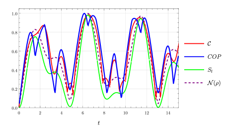
Figure 1: Complexity from operator-state mapping ($\mathcal{C}$), COP, Linear Entropy and Entanglement Negativity vs time for small $\lambda$ (i.e $\lambda<1$) when both the system and bath are regular oscillators ($\epsilon_{1}=\epsilon_{2}=1$ and $\lambda=0.5$).

We study and compare the time evolution of the subsystem complexity (both COP and complexity from operator-state mapping), linear entropy and entanglement negativity for different choices of system parameters. Below we list the main features and conclusion drawn from them.

• When both the system and bath are ordinary oscillators, all four quantities show oscillatory behavior and do not saturate as evident from Fig. 1. Moreover, the peaks appear around the same time for all the quantities.

• Entanglement negativity $\mathcal{N}(\rho)$ does not saturate for any values of coupling $\lambda$. Apart from the case shown in Fig. 1, when both the system and the bath is regular and the coupling is small ($\lambda<1$), it always grows exponentially with time as shown in Fig. 2. This can be contrasted with the behaviour of the linear entropy and complexity. When both the system and the bath are regular, then irrespective of the magnitude of $\lambda$ both the complexity and the linear entropy shows an oscillatory behaviour as demonstrated in the Fig. 1 and Fig. 3.

  

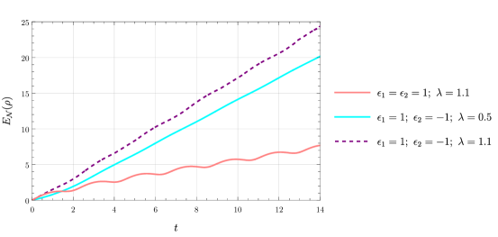
  Figure 2: Logarithmic Negativity vs time for different parameter choices in two-oscillator model (Note that, the entanglement negativity remains the same even if we exchange the values $\epsilon_{1}\leftrightarrow\epsilon_{2}$.)

• When either the bath or the system is inverted, both the complexity and the linear entropy reach to a saturation as shown in the Fig. 4 and Fig. 5. Interestingly both complexities (COP and complexity from state-operator mapping) reach to their saturation values faster than the linear entropy as evident from the Fig. 4 and Fig. 5. Moreover, we can also conclude that when the system becomes mixed, the complexity is expected to be saturated. We have extensively scanned the parameter space for this two-oscillator model.

  

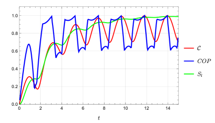
  Figure 3: Complexity from operator-state mapping ($\mathcal{C}$), COP and Linear Entropy vs time for large $\lambda$ (i.e $\lambda>1$) when both the system and bath are regular oscillators ($\epsilon_{1}=\epsilon_{2}=1$ and $\lambda=1.1$).

• Last but not the least, the exponential growth of entanglement negativity (or the linear growth of the logarithmic negativity as shown in Fig. 2) can be contrasted with the behaviour of both the complexities (from operator-state mapping and COP). The complexity saturates when either of the oscillator is inverted and the system gets maximally mixed. Note that the two-oscillator model is only a toy model. In the next section, we will see that for a more realistic model (Caldeira Leggett model) negativity will also saturate when the system becomes mixed.

  

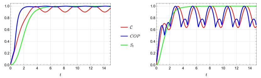
  Figure 4: Complexity from operator-state mapping ($\mathcal{C}$), COP and Linear Entropy vs time for small $\lambda$ when bath is inverted and system is normal ($\epsilon_{1}=1,\,\epsilon_{2}=-1)$ and $\lambda=0.5$ (Left) $\lambda=1.2$ (Right).

  

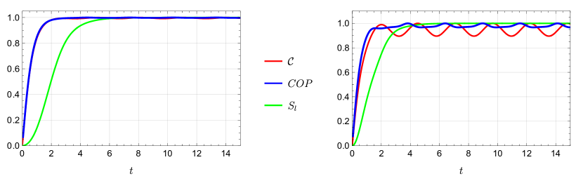
  Figure 5: Complexity from operator-state mapping ($\mathcal{C}$), COP and Linear Entropy vs time for small $\lambda$ when system is inverted and bath is normal ($\epsilon_{1}=-1,\,\epsilon_{2}=1)$ and $\lambda=0.5$ (Left) $\lambda=1.1$ (Right).

4.2 Caldeira Leggett Model

We now turn our attention to yet another simple model of open quantum system, namely the Caldeira Leggett model. The Caldeira Leggett model [115, 116] provides one of the first microscopic descriptions of Quantum Brownian motion. It’s a simple model where the dissipative dynamics of a harmonic oscillator interacting with a bosonic bath is captured by a position-position coupling. Below we review some details of our setup following [79]. Interested readers are referred to [79] for more details.

Solving the Model: In principle, there are two ways to model such a heat bath. One way is is to consider a reservoir composed of a large ensemble of non-interacting quantum systems such as harmonic oscillators and the second way is to use a free field. In this paper we will consider the second approach as in [117, 79]. Explicitly, the system we consider is a harmonic oscillator that is coupled to a one-dimensional free bosonic field. The Hamiltonian is given by

$$H=\int_{0}^{L}dx~{}\left\{\frac{1}{2}\left[\Pi^{2}+(\partial_{x}\phi)^{2}\right]+\delta(x)\left[\frac{1}{2}P^{2}+\frac{\omega^{2}_{0}}{2}Q^{2}+\lambda Q\partial_{x}\phi\right]\right\}\ ,$$ (55)

where we are ultimately interested in the $L\rightarrow\infty$ limit. In Eq. 55, $Q$ and $P$ are canonically conjugate variables describing the system, $[Q,P]=i$; $\phi$ and $\Pi$ are canonically conjugate fields of the bath, $[\phi(x),\Pi(x^{\prime})]=i\delta(x-x^{\prime})$. Furthermore, the field $\phi$ satisfies Dirichlet boundary conditions at $x=0$ and $x=L$:

$$\phi(x=0)=0;\hskip 28.45274pt\phi(x=L)=0.$$ (56)

For further simplification, we define the decay rate, $\Gamma\equiv\lambda^{2}/2$. We consider the following quench in the above model (Eq. 55) —

$$H=\left\{\begin{array}[]{c c c}H_{<}&{\rm for}&t<0\\ H_{>}&{\rm for}&t>0\end{array}\right.\ ,$$ (57)

In what follows, we start the system in the ground state of $H_{<}.$ We take $H_{<}$ to be the Hamiltonian of the system and bath decoupled.

$$H_{<}=\int_{0}^{L}dx~{}\frac{1}{2}\left[\Pi^{2}+(\partial_{x}\phi)^{2}\right]+\frac{1}{2}P^{2}+\frac{\Omega_{<}^{2}}{2}Q^{2}$$ (58)

By performing the following mode expansion [79],

$$\phi(x) = \sqrt{\frac{2}{L}}\sum_{n=1}^{\infty}\sin\left(\frac{\pi n}{L}x\right)\,\frac{1}{\sqrt{2\Omega_{n}}}(a^{\phantom{\dagger}}_{n}+a^{\dagger}_{n})\,,$$ (59)

$$\Pi(x) = -i\sqrt{\frac{2}{L}}\sum_{n=1}^{\infty}\sin\left(\frac{\pi n}{L}x\right)\,\sqrt{\frac{\Omega_{n}}{2}}(a^{\phantom{\dagger}}_{n}-a^{\dagger}_{n})$$ (60)

$$Q = \frac{1}{\sqrt{2\Omega_{<}}}(a_{0}+a_{0}^{\dagger})$$ (61)

$$P = -i\sqrt{\frac{\Omega_{<}}{2}}(a_{0}-a_{0}^{\dagger})\ ,$$ (62)

we get

$$H_{<}=\sum_{n=1}^{\infty}\frac{\pi\,n}{L}\left(a^{\dagger}_{n}a^{\phantom{\dagger}}_{n}+1/2\right)+\Omega_{<}\left(a_{0}^{\dagger}a_{0}^{\phantom{\dagger}}+1/2\right)\,.$$

Our initial state $|\psi_{0}\rangle$ is annihilated by the $\{a_{i}\}$:

$$a_{i}\mid\psi_{0}\rangle=0\ \ \forall\ i\,.$$ (63)

Then our final state is obtained by evolving $|\psi_{0}\rangle$ with $H_{>}$ and $H_{>}$ is given by Eq. 55.

$$|\psi(t)\rangle=e^{-i\,H_{>}\,t}|\psi_{0}\rangle.$$ (64)

We will consider two different sets of parameters:

• Underdamped oscillator : $\Omega^{2}>0$, i.e, $\omega_{0}^{2}>\Gamma^{2}$.

• Overdamped oscillator : $\Omega^{2}<0$, i.e, $\omega_{0}^{2}<\Gamma^{2}$.

To proceed further we first introduce a dual field $\theta$ such that

$$\Pi=-\partial_{x}\theta\,,$$ (65)

with $[\phi(x),\theta(x^{\prime})]=(i/2){\rm sgn}(x^{\prime}-x)$. In terms of these fields now the bath Hamiltonian takes the form [79],

$$H_{B}=\int_{0}^{L}dx~{}\frac{1}{2}\left[(\partial_{x}\theta)^{2}+(\partial_{x}\phi)^{2}\right]\ .$$

Now we decompose $\phi$ and $\theta$ into right and left movers

$$\phi(x)=\phi_{R}(x)+\phi_{L}(x)\ \ ,\ \ \theta(x)=\phi_{R}(x)-\phi_{L}(x)\ ,$$ (66a)

where $$\phi_{R} \phi_{L}$$ and satisfy the commutation relations

$$[\phi_{R}(x),\phi_{R}(x^{\prime})]=\frac{i}{4}{\rm sgn}(x-x^{\prime})\ \ ,\ \ [\phi_{L}(x),\phi_{L}(x^{\prime})]=-\frac{i}{4}{\rm sgn}(x-x^{\prime})\ \ ,\ \ [\phi_{R}(x),\phi_{L}(x^{\prime})]=0\ .$$ (66b)

In the Heisenberg picture, $\phi_{R}$ is a function of $(x-t)$, and $\phi_{L}$ is a function of $(x+t)$: $\phi_{R}(x,t)=\phi_{R}(x-t)$ and $\phi_{L}(x,t)=\phi_{L}(x+t)$. Using the Dirichlet boundary condition $\phi(x=0,t)=0$, we have $\phi_{L}(x=0,t)=-\phi_{R}(x=0,t)\,.$ This implies

$$\phi_{L}(x+t)=-\phi_{R}(-x-t)\ ,$$ (67a)

namely that $$\phi_{L} \phi_{R} x<0 \phi(x=L,t)=0$$ can be regarded as the continuation of to . Then using the boundary condition , one obtains

$$\phi_{R}(-L,t)=\phi_{R}(L,t)\ ,$$ (67b)

so that we can work with right-movers on the interval $-L<x<L$ satisfying periodic boundary conditions. For more details please refer to the Appendix B. Writing the full Hamiltonian defined in Eq. 55 solely in terms of right movers, we obtain [79],

$$H=\int_{-L}^{L}dx~{}\left\{(\partial_{x}\phi_{R})^{2}+\delta(x)\left[\frac{1}{2}P^{2}+\frac{\omega^{2}_{0}}{2}Q^{2}+2\lambda Q\partial_{x}\phi_{R}\right]\right\}\,.$$ (68)

From Eq. 68, we obtain the (Heisenberg) equations of motion for the operators

$$\partial_{t}\phi_{R}=-\partial_{x}\phi_{R}-\delta(x)\lambda Q\ \ ,\ \ \frac{d^{2}Q}{dt^{2}}+\omega^{2}_{0}Q=-2\lambda\partial_{x}\phi_{R}(0)\ .$$ (69)

The homogeneous part of the first equation in Eq. 69 tell us that, the $\phi_{R}$ is a function of $(x-t)$; using that as a “source” term acting only at $x=0$, we integrate about a small region about $x=0$: $-\epsilon<x<+\epsilon$. Eq. 69 becomes

$$0 = \phi^{+}_{R}(x=+\epsilon)-\phi^{-}_{R}(x=-\epsilon)\Big{|}_{\epsilon\rightarrow 0}+\lambda\,Q$$

$$\frac{d^{2}Q}{dt^{2}}+\omega^{2}_{0}Q = -\lambda\left[\partial_{x}\phi^{+}_{R}(x=0)+\partial_{x}\phi^{-}_{R}(x=0)\right]\ ,$$ (70)

where we have introduced the notation $\phi^{+}_{R}(x)\equiv\phi_{R}(x>0)$ and $\phi^{-}_{R}(x)\equiv\phi_{R}(x<0)$.

We will apply the scattering formalism [118] to solve Eq. 70. In this formalism, we consider particles incoming from $x<0$, then they are scattered by the system at $x=0$, and finally are outgoing for $x>0$. From the practical point of view, we solve for $Q$ and $\phi^{+}_{R}$ in terms of $\phi^{-}_{R}$. Finally we get

$$\frac{d^{2}Q}{dt^{2}}+\omega_{0}^{2}Q+2\Gamma\,\frac{dQ}{dt}=2\sqrt{2\Gamma}\,\frac{d\phi_{R}^{-}}{dt},$$ (71)

where $\Gamma=\lambda^{2}/2$. The solution for $Q(t)$ can be written as

$$Q(t)=Q_{H}(t)+Q_{P}(t),$$ (72)

where, $Q_{H}(t)$ and $Q_{P}(t)$ are the homogeneous and particular solutions respectively. The homogeneous solution turns out to be the following:

$$Q_{H}(t) = e^{-\Gamma t}\left\{[\cos\Omega t+\left(\frac{\Gamma}{\Omega}\right)\sin\Omega t]Q(t=0)+(1/\Omega)\sin\Omega t~{}P(t=0)\right\}$$ (73)

$$- e^{-\Gamma t}\left\{[\cos\Omega t+\left(\frac{\Gamma}{\Omega}\right)\sin\Omega t]Q_{P}(t=0)+(1/\Omega)\sin\Omega t~{}\dot{Q}_{P}(t=0)\right\}\ ,$$

where $\Omega=\sqrt{\omega_{0}^{2}-\Gamma^{2}}$. To find the particular solution we introduce the Fourier transforms

$$\phi_{R}(x,t)=\int\frac{d\omega}{\sqrt{2\pi}}e^{-i\omega(t-x)}\phi_{R}(\omega)\ \ ,\ \ Q(t)=\int\frac{d\omega}{\sqrt{2\pi}}e^{-i\omega t}Q(\omega)\ ,$$ (74)

and obtain

$$Q_{P}(\omega) =\left(\frac{i2\sqrt{2\Gamma}\omega}{\omega^{2}+i2\Gamma\omega-\omega_{0}^{2}}\right)\phi_{R}^{-}(\omega)\ ,$$ (75)

$$\phi_{R}^{+}(\omega) =-\sqrt{2\Gamma}\ Q_{H}(\omega)+\left(\frac{\omega^{2}-i2\Gamma\omega-\omega_{0}^{2}}{\omega^{2}+i2\Gamma\omega-\omega_{0}^{2}}\right)\phi_{R}^{-}(\omega)\ .$$

To execute calculations for the bath, one must understand $\phi_{R}^{-}(\omega)$ as

$$\phi_{R}^{-}(\omega)=\left\{\begin{array}[]{c c c}\frac{a^{\phantom{\dagger}}_{\omega}}{\sqrt{2\omega}}&{\rm for}&\omega>0\\ \frac{a^{\dagger}_{\omega}}{\sqrt{2|\omega|}}&{\rm for}&\omega<0\\ \end{array}\right.\ ,$$

namely, that $\phi_{R}^{-}(\omega)$ is an annihilation operator for $\omega>0$ and a creation operator for $\omega<0$ (with a prefactor $1/\sqrt{2|\omega|}$). Finally, the bosonic bath fields $\phi(x,t)$ and $\Pi(x,t)$ can be expressed as:

$$\phi(x,t) =\phi_{0}(x,t)-{\rm sgn}{(x)}\,\lambda Q(t-|x|)$$ (76)

$$\Pi(x,t) =\Pi_{0}(x,t)-{\rm sgn}{(x)}\,\lambda\dot{Q}(t-|x|)$$ (77)

where, $\phi_{0}(x,t)$ and $\Pi_{0}(x,t)$ are the time evolution of the bosonic fields in the free theory, i.e,

$$\phi_{0}(x,t) \equiv-i\,\int_{0}^{\infty}\frac{d\omega}{\sqrt{\pi\omega}}\,\sin{(\omega x)}\,\left(a_{\omega}^{\dagger}e^{i\omega t}-a_{\omega}e^{-i\omega t}\right)\,,$$ (78)

$$\Pi_{0}(x,t) \equiv\int_{0}^{\infty}d\omega\,\sqrt{\frac{\omega}{\pi}}\,\sin{(\omega x)}\,\left(a_{\omega}^{\dagger}e^{i\omega t}+a_{\omega}e^{-i\omega t}\right)\,.$$

After knowing the solutions mentioned in Eq. 73, 75 and 76, we are now in a position to compute the time-evolved wavefunction mentioned in Eq. 64.

Reduced Density Matrix for the Oscillator (system): In this paper we are interested in the reduced density matrix of the system by tracing out the bath degrees of freedom. To obtain that, we divide the full system into two subsystems-oscillator and the string and then traced out the string.

$$\hat{\rho_{S}}={\rm Tr}_{B}[\hat{\rho}]\ ,$$ (79)

where $\hat{\rho}$ is the density matrix of the entire system. The subscript $S$ and $B$ implies system and bath respectively. The system starts from the ground state of the uncoupled Hamiltonian defined in Eq. 58. Then we time evolve it by $H_{>}$ defined in Eq. 57. As the initial density matrix is Gaussian and the Hamiltonian is quadratic, the density matrix remains Gaussian for all times. In the position representation, it has the following structure

$$\rho_{S}(x,x^{\prime})=\sqrt{\frac{\gamma_{1}-\eta}{\pi}}\exp\left\{-\frac{\gamma}{2}x^{2}-\frac{\gamma^{*}}{2}x^{\prime 2}+\eta\,lxx^{\prime}\right\}\ ,$$ (80)

where $\gamma\ (=\gamma_{1}+i\gamma_{2})\in{\bf C}$ and $\eta\in{\bf R}$.

The parameters $\{\gamma,\eta\}$ can be obtained from the system’s correlation functions. As the density matrix is Gaussian, it is fully characterized by its first and second moments. It can be easily checked that, the initial wave function mentioned in Eq. 63, the folloiwng expectation values vanish.

$$\langle Q\rangle=0\quad\textrm{and}\quad\langle P\rangle=0.$$

Then due to the structure of the Hamiltonian, this is preserved for all times. The parameters in the density matrix defined in Eq. 80 are given in terms of two point correlators of canonical variables $Q$ and $P$ describing the single oscillator [79],

$$\gamma_{1}=\sigma_{P}-\frac{1}{\sigma_{Q}}\left(\sigma_{QP}^{2}-1/4\right)\ \ ,\ \ \gamma_{2}=-\frac{\sigma_{QP}}{\sigma_{Q}}\ \ ,\ \ \eta=\sigma_{P}-\frac{1}{\sigma_{Q}}\left(\sigma_{QP}^{2}+1/4\right)\ ,$$ (81)

where

$$\sigma_{Q}=\langle Q(t)Q(t)\rangle\ \ ,\ \ \sigma_{P}=\langle P(t)P(t)\rangle\ \ ,\ \ \sigma_{QP}=\frac{1}{2}\langle Q(t)P(t)+P(t)Q(t)\rangle\ \ ;$$ (82)

Interested readers are referred to Appendix C and D for the details of the computation of these correlators.

Linear Entropy, Negativity and Complexity for Caldeira Leggett Model: Once we have the $\gamma$ and $\eta$ as defined in Eq. 80, we follow the same procedure outlined for the two oscillator case in Sec. 4.1 to compute linear entropy, negativity and complexities. Linear entropy is $S_{l}$ is given for this case by the Eq. 32

Next we compute the entanglement negativity following the procedure as discussed in Section 2 for two-mode Gaussian state. First we need to compute first the density matrix for the full system (i.e for oscillator and the bath together). Since this is also of the Gaussian form it is completely characterised by its first and second moments as mentioned earlier. All the first moment vanishes because of our choice of the initial state as mentioned earlier. Then we compute the covariance matrix as defined in Eq. 7. Note that the term $\delta(x)\,\lambda\,Q\,\partial_{x}\phi$ in the Hamiltonian (Eq. 55) denotes the interaction between the bosonic bath $\phi(x)$ and the harmonic oscillator $Q$ to be only at $x=0$. Therefore, we consider the following canonical phase-space variables describing the system and bath,

$$X_{i}=\{Q,\,P,\,{\phi(x=0)},\,{\Pi(x=0)}\}.$$

We have already computed the correlators corresponding to system variables $Q(t),P(t)$. To compute the negativity, in addition to the system correlators, we now need to compute the two point correlators of system-bath and bath variables. However, the boundary conditions on $\phi(x)$ defined in Eq. 56 sets ${\phi(0)}={\Pi(0)}=0$, and the corresponding correlators become zero. As a result, the negativity becomes undefined. Therefore we introduce a small length parameter $\delta\ll L$, and consider the bosonic fields at $x=\delta$. Then we can compute the correlators between the phase-space variables $\{Q,\,P,\,{\phi(x=\delta)},\,{\Pi(x=\delta)}\}$ (see Appendix D), and construct the covariance matrix $\sigma_{ij}$ as defined in Eq. 7. By using this covariance matrix (Eq. 7) we can calculate the negativity using Eq. 9.

Lastly, we compute the complexities- COP and complexity from operator-state mapping. Just like the two-oscillator model COP for this case also given by Eq. 50, with following identification,

$$\alpha=\sigma_{P},~{}~{}\tau^{2}=4\,\sigma^{2}_{QP}-1+4\,i\,\sigma_{QP},~{}~{}{\rm Re}(\gamma)=2\,\sigma_{Q},$$ (83)

where $\sigma_{Q},\sigma_{P},\sigma_{QP}$ are defined in Eq. 81. Also in all the subsequent analysis we will set the reference frequency to be $\omega_{0}=1$ following [79]. Last but not the least, to compute the circuit complexity using operator-state mapping, we start with the reduced density matrix of the oscillator as mentioned in Eq. 80. As mentioned earlier we are mostly interested in $\hat{\rho}_{s}^{1/2}$ and the corresponding corresponding effective wavefunction will be of the form mentioned in Eq. 51 and Eq. 52. After that the complexity can be computed using Eq. A.8.

4.2.1 Time Evolution of Linear Entropy, Negativity and Complexity

In this section we investigate in details the saturation time scale for complexity, linear entropy and negativity. We have scanned the parameter space in detail. Below we pointwise summarize our results.

• For both underdamped and overdamped cases we find that all four quantities saturate almost at the same time scale. The results are shown in Fig. 6 (weak coupling, hence under damped) and Fig. 7 (strong coupling, hence over damped).

  

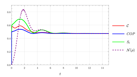
  Figure 6: Complexity, Negativity and Linear Entropy vs time, by choosing $\omega_{0}=1$ and $\Gamma=0.3$ in Caldeira Legget Model for Underdamped Oscillator.

  

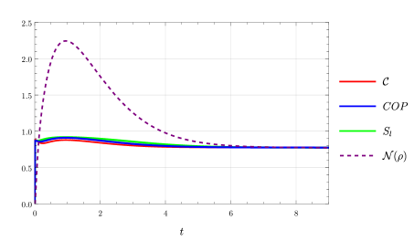
  Figure 7: Complexity, Negativity and Linear entropy vs time, by choosing $\Omega=1;~{}\Gamma=1.2$ in Caldeira Legget Model for Overdamped Oscillators :

• Just like our previous model (the two-oscillator model), we find a similar behaviour for the time scales of linear entropy and complexity. When the system becomes completely mixed–linear entropy saturates, both COP and complexity by operator state mapping is already saturated. The saturation time scale for complexity is smaller than the saturation time scale for linear entropy. So we can arrive at the same conclusion that, the complexity saturates when the system is maximally mixed. However, unlike the two oscillator model, the linear entropy and entanglement negativity have the same saturation time scale. This implies that for this model when the system is completely mixed then the quantum correlation/entanglement between the system and the bath also saturates. Therefore, entanglement negativity can detect when the system becomes mixed.

• Furthermore, our results imply that the complexity is more sensitive in detecting mixedness. To compute these quantities, we have computed various two-point correlators and used a cutoff to control various divergences that appear in these correlators. Details of the computation is mentioned in Appendix D. Moreover, as mentioned previously, we introduced a small length parameter $\delta$, and considered the bosonic bath fields at $x=\delta$ to compute the additional correlators. However, the saturation time scales do not depend on the choice of $\delta$ as shown in Fig. 8, thereby making our claim about the saturation time scale universal.

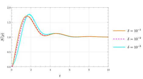
Figure 8: Negativity vs time for different choices of $\delta$ (when $\omega_{0}=1$ and $\Gamma=0.3$). The saturation value of $\mathcal{N}(\rho)$ is normalized to 1 in each plot.

5 Discussion

In this paper, we considered two different open quantum systems and compared the saturation time scale for complexity, linear entropy and entanglement negativity. Our first model, two coupled oscillators, is basically a toy model for open quantum system and the entanglement negativity does not saturate for this model. However, for a more realistic Caldeira Leggett model, we found that the time scale when the entanglement negativity saturates is of the same order as the time scale when the system is maximally mixed, i.e. linear entropy also saturates. The quantum correlation between the system and the bath saturates when the system becomes maximally mixed.

On top of this, we discovered that complexity saturates a bit earlier than the above saturation time scale of linear entropy for both the two-oscillator and Caldeira Leggett model, implying that complexity is already maximum when the system is completely mixed . We have thoroughly scanned the parameter space and found that these saturation time scales are independent of the regularization scheme (Caldeira Leggett model). All of these point to the universal nature of our results.

It will be interesting to generalize our computation for multi-oscillator (more than two) systems. One can start with a Caldeira Leggett type of model, but the model the bath by considering the sum of many oscillators. Also, in this paper, we have considered the Caldeira Leggett model with the Dirichlet boundary condition. It will be worthwhile to understand the effect of the boundary condition; hence it will be interesting to repeat this study for other boundary conditions, e.g. Neumann boundary condition. Note that, in this paper, we have computed the entanglement negativity for full density matrix, i.e. system and bath combined. It will be interesting to increase the size of the system and compute the negativity for the system after bipartisan it and tracing out the bath. This will generate a true mixed state corresponding to the system, and then it will be interesting to study how the evolution of negativity for this mixed state. Suppose the system initially has some quantum correlation. In that case, studying the time of evolution negativity will help us understand how the initial quantum correlation changes when there is an interaction with the bath.

Furthermore, it will be very interesting to extend this study to conformal field theory (CFT). Some studies regarding decoherence dynamics for CFT and time evolution of entanglement negativity and purity have been done here [25]. It will be good to again compare the saturation time scales of these quantities with the corresponding complexity. This will open up the possibility of connecting with gravity by making use of the AdS/CFT correspondence .

Last but not least, there are other notions of complexity, e.g. Krylov complexity [119], which measures operator growth under time evolution. Perhaps it is interesting to study this notion of complexity for the system we considered in this paper and investigate (perhaps along the line of [120]) whether it can tell us anything about the system being mixed or not. Apart from this, one perhaps also study other measures of correlation, e.g. out-of-time-ordered correlator [121, 122, 123, 124], the entanglement of purification [109, 110] for this kind of open systems and compare with the behaviour complexity, linear entropy and negativity that we have studied here. We hope to get back to some of these questions in a future publication.

Appendix A Circuit Complexity

In this we will briefly review some aspects of computation of circuit complexity. We will use the Nielsen’s method [75, 76, 77]. Further details can be found in [31]. The question we explore is the following: given a reference state and set of elementary quantum gates, what is the most efficient way to get a target state. Namely, how to find the most efficient quantum circuit that starts at that reference state (at $s=0$) and terminates at a target state ($s=1$)

$$|\Psi_{s=1}\rangle=U(s=1)|\Psi_{s=0}\rangle,$$ (A.1)

where $U$ is the unitary operator that takes the reference state to the target state. We will represent the target sate $|\Psi_{s=1}\rangle$ as $|\Psi_{T}\rangle$ and the reference state $|\Psi_{s=0}\rangle$ as $|\Psi_{R}\rangle$ in the rest of the paper. We construct it from a continuous sequence of parametrized path ordered exponential of a control Hamiltonian operator

$$U(s)={\overleftarrow{\mathcal{P}}}\exp[-i\int_{0}^{s}ds^{\prime}H(s^{\prime})]\ .$$ (A.2)

Here $s$ parametrizes a path in the space of the unitaries and given a set of elementary gates $M_{I}$, the control Hamiltonian can be written as

$$H(s)=Y^{I}(s)M_{I}\,.$$ (A.3)

The coefficients $Y^{I}$ are the control functions that dictates which gate will act at a given value of the parameter. The control function is basically a tangent vector in the space of unitaries and satisfy the Schrodinger equation

$$\frac{dU(s)}{ds}=-i\,Y^{I}(s)M_{I}U(s)\,.$$ (A.4)

Then we define a cost functional $\mathcal{F}(U,\dot{U})$ as follows :

$${\mathcal{C}}(U)=\int_{0}^{1}\mathcal{F}(U,\dot{U})ds\,.$$ (A.5)

Minimizing this cost functional gives us the optimal circuit. There are different choices for the cost functional [31]. In this paper we will consider

$$\mathcal{F}_{2}(U,Y)=\sqrt{\sum_{I}(Y^{I})^{2}}\,.$$ (A.6)

In this paper, the target wave function $\psi_{T}(x_{1},x_{2})=\langle x_{1},x_{2}|\psi_{T}\rangle$ takes the following form, takes the following form

$$\psi_{T}(x_{1},x_{2})={\cal N}(t)\exp\left(-\frac{1}{2}\left[\Omega_{1}(t)x_{1}^{2}+\Omega_{2}(t)x_{2}^{2}-2\,\kappa(t)x_{1}x_{2}\right]\right)\ ,$$ (A.7)

where $\Omega_{1}(t)$, $\Omega_{2}(t)\in{\bf C}$ (with ${\rm Re}[\Omega_{1}(t)]$, ${\rm Re}[\Omega_{2}(t)]>0$) and $\kappa(t)$, ${\cal N}(t)\in{\bf R}$. For the reference state $\psi_{R}(x_{1},x_{2})$ $\Omega_{1}(t=0)=\Omega_{2}(t=0)=1$ and $\kappa(t=0)=0\,.$ Following [35], we will take the elementary gates $M_{I}$ as the generators of the $GL(2,C)$ group. For details interested readers are referred to [35]. In all the cases, the complexity takes the form [35] (due to the structure of the wave functions)

$$\mathcal{C}=\frac{1}{2}\sqrt{\sum_{\alpha=1,2}\left(\ln\left(|\hat{\Omega}_{\alpha}|\right)^{2}+\tan^{-1}\left(-\frac{\text{Im}(\hat{\Omega}_{\alpha})}{\text{Re}(\hat{\Omega}_{\alpha})}\right)^{2}\right)}\ ,$$ (A.8)

where $\alpha=1,2$ and the normal mode frequencies are given by,

$$\begin{split}&\hat{\Omega}_{1}=\frac{1}{2}\Big{(}\Omega_{1}(t)+\Omega_{2}(t)+\sqrt{(\Omega_{1}(t)-\Omega_{2}(t))^{2}+4\kappa(t)^{2}}\Big{)},\\ &\hat{\Omega}_{2}=\frac{1}{2}\Big{(}\Omega_{1}(t)+\Omega_{2}(t)-\sqrt{(\Omega_{1}(t)-\Omega_{2}(t))^{2}+4\kappa(t)^{2}}\Big{)}.\end{split}$$ (A.9)

Appendix B Mode expansion for Caldeira Leggett Model and Periodic Boundary Conditions

Here we give some details of the mode expansion of the bath Hamiltonian [79]. The Hamiltonian is given by,

$$H=\frac{1}{2}\int_{0}^{L}dx\left[\Pi^{2}+(\partial_{x}\phi)^{2}\right]\ .$$ (B.1)

The field $\phi$ satisfies the periodic boundary condition $\phi(x+L)=\phi(x)$. By introducing the mode expansions

$$\phi(x)=\frac{1}{\sqrt{L}}\sum_{k}e^{ikx}\frac{1}{\sqrt{2\Omega_{k}}}(a^{\phantom{\dagger}}_{k}+a^{\dagger}_{-k})\ \ ,\ \ \Pi(x)=-i\frac{1}{\sqrt{L}}\sum_{k}e^{ikx}\sqrt{\frac{\Omega_{k}}{2}}(a^{\phantom{\dagger}}_{k}-a^{\dagger}_{-k})\ ,$$ (B.2)

where $k=(2\pi/L)n$ with $n\in{\bf Z}$, and $\Omega_{k}=|k|$, we can diagonalize the Hamiltonian

$$H=\sum_{k}\Omega_{k}(a^{\dagger}_{n}a^{\phantom{\dagger}}_{n}+1/2)\ .$$ (B.3)

Then we introduce the dual field $\theta$ such that $\Pi=-\partial_{x}\theta$. The mode expansion for $\theta$ is given by

$$\theta(x)=\frac{1}{\sqrt{L}}\sum_{k}e^{ikx}\frac{\rm sgn(k)}{\sqrt{2\Omega_{k}}}(a^{\phantom{\dagger}}_{k}-a^{\dagger}_{-k})\ .$$ (B.4)

Finally, one introduces the chiral fields $\phi_{R}$ and $\phi_{L}$, such that

$$\phi=\phi_{R}+\phi_{L}\ \ ,\ \ \theta=\phi_{R}-\phi_{L}\ ;$$ (B.5)

using the mode expansions for $\phi$ and $\theta$, one obtains

$$\phi_{R}(x)=\frac{1}{\sqrt{L}}\sum_{k>0}\frac{1}{\sqrt{2\Omega_{k}}}\left(e^{ikx}a^{\phantom{\dagger}}_{k}+e^{-ikx}a^{\dagger}_{k}\right)\ \ ,\ \ \phi_{L}(x)=\frac{1}{\sqrt{L}}\sum_{k>0}\sqrt{\frac{\Omega_{k}}{2}}\left(e^{-ikx}a^{\phantom{\dagger}}_{-k}+e^{ikx}a^{\dagger}_{-k}\right)\ .$$ (B.6)

We are ultimately interested in $L\rightarrow\infty$ — Eq. B.6 becomes

$$\phi_{R}(x)=\int_{0}^{\infty}\frac{d\omega}{\sqrt{2\pi}}\frac{1}{\sqrt{2\omega}}\left(e^{i\omega x}a^{\phantom{\dagger}}_{\omega}+e^{-i\omega x}a^{\dagger}_{\omega}\right)\ \ ,\ \ \phi_{L}(x)=\int_{0}^{\infty}\frac{d\omega}{\sqrt{2\pi}}\frac{1}{\sqrt{2\omega}}\left(e^{-i\omega x}a^{\phantom{\dagger}}_{-\omega}+e^{i\omega x}a^{\dagger}_{-\omega}\right)\ .$$

Appendix C Characteristic Function

We now spell out some details about the the characteristic function following [79] to make this paper self-contained. By using the density matrix

$$\rho(Q,Q^{\prime})=\mathcal{N}{\rm exp}\left\{-\frac{1}{2}\left(\alpha Q^{2}+\alpha^{*}Q^{\prime 2}-cQQ^{\prime}\right)\right\},$$ (C.1)

where $\alpha=(\alpha_{1}+i\alpha_{2})\in\mathbf{C}$ and $c\in\mathbf{R}$, one can find the $l$’th moment for an arbitrary operator $\mathcal{O}$ as follows

$$\langle\mathcal{O}^{l}\rangle={\rm tr}(\rho\,\mathcal{O}^{l})\,.$$ (C.2)

By defining a characteristic function as follows

$${\rm CF}(\epsilon,t)\equiv{\rm tr}(\rho\,e^{-i\epsilon\mathcal{O}}),$$ (C.3)

where $\epsilon$ is a real parameter, we can find the moments of all orders

$$\langle\mathcal{O}^{l}(t)\rangle=\frac{\partial^{l}}{\partial(i\epsilon)^{l}}{\rm CF}(\epsilon,t)\ \Big{|}_{\epsilon=0}\,.$$ (C.4)

Now, a characteristic function for the position and momentum operators can be written in terms of creation and annihilation operators $a$ and $a^{\dagger}$ as follows:

$${\rm CF}(\epsilon,t)\equiv{\rm tr}(\rho e^{-i\eta(\epsilon a+\epsilon^{*}a^{\dagger})}),$$ (C.5)

where $\epsilon\in\mathbb{C}$ and $\eta\in\mathbb{R}$. This is also known as the Wigner characteristic function.

The creation and annihilation operators are

$$a=\frac{1}{\sqrt{2\Omega}}(\Omega Q+iP)\ ,\ \ a^{\dagger}=\frac{1}{\sqrt{2\Omega}}(\Omega Q-iP).$$ (C.6)

By using Eq. C.6 we can write

$${\rm CF}(\lambda,\mu)\equiv{\rm tr}(\rho\ e^{-i(\lambda Q+\mu P)}),$$ (C.7)

where $\lambda=\eta(\epsilon+\epsilon^{*})\sqrt{\Omega/2}$ and $\mu=i\eta(\epsilon-\epsilon^{*})/(\sqrt{2\Omega})$. By using the commutation relation $([Q,P]=i)$, the exponent in Eq. C.7 can be expanded as

$$e^{-i(\lambda Q+\mu P)} = e^{-i\lambda Q}e^{-i\mu P}e^{\frac{1}{2}i\lambda\mu}$$ (C.8)

$$= e^{-\frac{1}{2}i\mu P}e^{\frac{1}{2}i\mu P}e^{-i\lambda Q}e^{-\frac{1}{2}i\mu P}e^{-\frac{1}{2}i\mu P}e^{\frac{1}{2}i\lambda\mu}$$

$$= e^{-\frac{1}{2}i\mu P}e^{-i\lambda(Q+\frac{\mu}{2})}e^{-\frac{1}{2}i\mu P}e^{\frac{1}{2}i\lambda\mu}$$

$$= e^{-\frac{1}{2}i\mu P}e^{-i\lambda Q}e^{\frac{1}{2}i\mu P}\,.$$

Now we will evaluate the trace in the position representation, where

$$Q|Q^{\prime}\rangle = Q^{\prime}|Q^{\prime}\rangle\,,$$ (C.9)

$$\langle Q^{\prime}|Q^{\prime\prime}\rangle = \delta(Q^{\prime}-Q^{\prime\prime})\,,$$ (C.10)

$$\int_{-\infty}^{\infty}dQ^{\prime}|Q^{\prime}\rangle\langle Q^{\prime}| = 1\,.$$ (C.11)

Furthermore,

$$e^{\frac{1}{2}i\mu P}|Q^{\prime}\rangle = {\Big{|}}Q^{\prime}-\frac{\mu}{2}{\Big{\rangle}}\,,$$ (C.12)

$$\langle Q^{\prime}|\ e^{\frac{1}{2}i\mu P} = {\Big{\langle}}Q^{\prime}+\frac{\mu}{2}{\Big{|}}\,.;$$ (C.13)

Using these we get from C.7

$${\rm CF}(\lambda,\mu) = {\rm tr}\ e^{-\frac{1}{2}i\mu P}\rho\ e^{-\frac{1}{2}i\mu P}e^{-i\lambda Q}$$ (C.14)

$$= \int e^{-i\lambda Q^{\prime}}{\Big{\langle}}Q^{\prime}-\frac{\mu}{2}|\rho|Q^{\prime}+\frac{\mu}{2}{\Big{\rangle}}dQ^{\prime}\,.$$ (C.15)

Now plugging the density matrix (Eq. C.1) in the above expression and performing the gaussian integrals we get

$${\rm CF}(\lambda,\mu)={\rm exp}\left\{-\frac{A}{2}\lambda^{2}-\frac{A^{\prime}}{2}\mu^{2}+B\mu\lambda\right\}\,,$$ (C.16)

where the parameters $A,A^{\prime}$ and $B$ are

$$A = \frac{1}{2(\alpha_{1}-c)}\,,$$ (C.17)

$$A^{\prime} = \frac{|\alpha|^{2}-c^{2}}{2(\alpha_{1}-c)}\,,$$ (C.18)

$$B = -\frac{\alpha_{2}}{2(\alpha_{1}-c)}.$$ (C.19)

These parameters are related to the correlators as follows:

$$\langle QQ\rangle = -\frac{\partial^{2}}{\partial\lambda^{2}}{\rm CF(\lambda,\mu)}{\Big{|}}_{\mu=\lambda=0}=A\,,$$ (C.20)

$$\langle PP\rangle = -\frac{\partial^{2}}{\partial\mu^{2}}{\rm CF(\lambda,\mu)}{\Big{|}}_{\mu=\lambda=0}=A^{\prime}\,,$$ (C.21)

$$\frac{1}{2}\langle QP+PQ\rangle = -\frac{\partial^{2}}{\partial\mu\partial\lambda}{\rm CF(\lambda,\mu)}{\Big{|}}_{\mu=\lambda=0}=B\,.$$ (C.22)

Appendix D Correlation Functions of Caldeira Leggett Model

We need compute the full system two-point correlators $\langle\hat{O}_{\alpha}(t_{1})\hat{O}_{\beta}(t_{2})\rangle$, where $\hat{O}_{\alpha,\beta}$ = $Q$, $P$, $\phi$ or $\Pi$ for computing various quantities mentioned in the main text. In this regard the correlators relating $Q_{p}(t)$, $\phi_{0}(\delta,t)$ and $\Pi_{0}(\delta,t)$ plays an important role. Following [79], we have

$$Q_{P}(t)=\int_{0}^{\infty}\frac{d\omega}{\sqrt{2\pi}}\frac{1}{\sqrt{2\omega}}\left[f(\omega)e^{-i\omega t}a^{\phantom{\dagger}}_{\omega}+f(-\omega)e^{i\omega t}a^{\dagger}_{\omega}\right]\ \ {\rm with}\ \ f(\omega)=\frac{i\omega\,2\sqrt{2\Gamma}}{\omega^{2}+i2\Gamma\omega-\omega_{0}^{2}}\ .$$ (D.1)

Using that the bath is taken to be initially in its ground state, we obtain

$$\langle Q_{p}(t_{1})Q_{p}(t_{2})\rangle=\frac{2\Gamma}{\pi}\int_{0}^{\infty}d\omega~{}e^{-i\omega(t_{1}-t_{2})}\frac{\omega}{(\omega^{2}-\omega_{0}^{2})^{2}+(2\Gamma\omega)^{2}}\ .$$

Carrying out the integral(s), we obtain the following,

$$\langle Q_{p}(t_{1})Q_{p}(t_{2})\rangle = I_{1}+iI_{2}$$ (D.2)

where

$$I_{1} = -\frac{1}{4\pi\sqrt{\Gamma^{2}-\omega_{0}^{2}}}\left(2\left[\sin(\tau\omega_{+}){\rm Si}(\tau\omega_{+})-\sin(\tau\omega^{*}_{+}){\rm Si}(\tau\omega^{*}_{+})\right]\right.$$

$$\left.+\cos(\tau\omega_{+})\left[{\rm Ci}(\tau\omega_{+})+{\rm Ci}(-\tau\omega_{+})\right]-\cos(\tau\omega^{*}_{+})\left[{\rm Ci}(\tau\omega^{*}_{+})+{\rm Ci}(-\tau\omega^{*}_{+})\right]\right)\ ,$$

$$I_{2} = \frac{1}{i(4\sqrt{\Gamma^{2}-\omega_{0}^{2}})}\left(\sin(\omega_{+}\tau)-\sin(\omega_{+}^{*}\tau)\right)\ .$$ (D.3)

In Eq. D,

$$\omega_{+}=\sqrt{\omega_{0}^{2}+\ 2\Gamma(-\Gamma+\sqrt{\Gamma^{2}-\omega_{0}^{2}})},\omega_{+}^{*}=\sqrt{\omega_{0}^{2}-2\Gamma(-\Gamma+\sqrt{\Gamma^{2}-\omega_{0}^{2}})},$$

$\tau=t_{1}-t_{2}$, and ${\rm Si}(z)$ (${\rm Ci}(z)$) is the sine-integral (cosine-integral) function [125]. We also compute the other correlators [79]:

$$\langle\dot{Q}_{p}(t_{1})Q_{p}(t_{2})\rangle = J_{1}+iJ_{2},$$ (D.4)

where

$$J_{1} = -\frac{1}{4\sqrt{2}\pi\sqrt{\Gamma^{2}-\omega_{0}^{2}}}\left\{2\left[\omega_{+}\cos(\tau\omega_{+}){\rm Si}(\tau\omega_{+})-\omega^{*}_{+}\cos(\tau\omega^{*}_{+}){\rm Si}(\tau\omega^{*}_{+})\right]\right.$$

$$\left.-\omega_{+}\sin(\tau\omega_{+})\left[{\rm Ci}(\tau\omega_{+})+{\rm Ci}(-\tau\omega_{+})\right]+\omega^{*}_{+}\sin(\tau\omega^{*}_{+})\left[{\rm Ci}(\tau\omega^{*}_{+})+{\rm Ci}(-\tau\omega^{*}_{+})\right]\right\}\ ,$$

$$J_{2} = \frac{1}{i(4\sqrt{\Gamma^{2}-\omega_{0}^{2}})}\left(\omega_{+}\cos(\omega_{+}\tau)-\omega_{+}^{*}\cos(\omega_{+}^{*}\tau)\right).$$ (D.5)

Similarly we get

$$\langle\dot{Q}_{p}(t_{1})\dot{Q}_{p}(t_{2})\rangle = K_{1}+iK_{2},$$ (D.6)

where

$$K_{1} = -\frac{1}{8\pi\sqrt{\Gamma^{2}-\omega_{0}^{2}}}\left\{2\left[\omega_{+}^{2}\sin(\tau\omega_{+}){\rm Si}(\tau\omega_{+})-\omega^{*2}_{+}\sin(\tau\omega^{*}_{+}){\rm Si}(\tau\omega^{*}_{+})\right]\right.$$

$$\left.+\omega_{+}^{2}\cos(\tau\omega_{+})\left[{\rm Ci}(\tau\omega_{+})+{\rm Ci}(-\tau\omega_{+})\right]-\omega^{*2}_{+}\cos(\tau\omega^{*}_{+})\left[{\rm Ci}(\tau\omega^{*}_{+})+{\rm Ci}(-\tau\omega^{*}_{+})\right]\right\}\ ,$$

$$K_{2} = \frac{1}{i(4\sqrt{\Gamma^{2}-\omega_{0}^{2}})}\left(\omega_{+}^{2}\sin(\omega_{+}\tau)-\omega_{+}^{*2}\sin(\omega_{+}^{*}\tau)\right)\,.$$ (D.7)

Lastly,

$$\langle Q(t_{1})Q_{p}(t_{2})\rangle = 0$$ (D.8)

and the correlators at time $t=0$:

$$\langle QQ\rangle=\frac{1}{2\Omega},\ \ \ \langle\dot{Q}\dot{Q}\rangle=\frac{1}{2\Omega}.$$ (D.9)

Note that to carry out the computations discussed in the paper, we need equal time correlators as mentioned in Eq. 81. But in the limit $t_{1}\rightarrow t_{2}$, they are typically divergent. To regularize the integral, we have used a cutoff $\tau_{c}.$

The correlators with the (free) bosonic fields, $\phi_{0}(\delta,t)$ and $\Pi_{0}(\delta,t)$, can be calculated to be:

$$\langle\phi_{0}\,\phi_{0}\rangle =\int_{0}^{\infty}\frac{d\omega}{\pi\omega}\,\sin^{2}{(\omega\delta)}$$ (D.10)

$$\langle\Pi_{0}\,\Pi_{0}\rangle =\int_{0}^{\infty}d\omega\,\frac{\omega}{\pi}\,\sin^{2}{(\omega\delta)}$$ (D.11)

$$\langle\phi_{0}\,\Pi_{0}+\Pi_{0}\,\phi_{0}\rangle =0$$ (D.12)

$$\langle\phi_{0}\,Q_{P}+Q_{P}\,\phi_{0}\ \rangle =\int_{0}^{\infty}\frac{d\omega}{\pi\omega}\,\sin{(\omega\delta)}\,{\rm Im}\left[f(\omega)\right]$$ (D.13)

$$\langle\phi_{0}\,\dot{Q}_{P}+\dot{Q}_{P}\,\phi_{0}\ \rangle =\int_{0}^{\infty}\frac{d\omega}{\pi}\,\sin{(\omega\delta)}\,{\rm Re}\left[f(\omega)\right]$$ (D.14)

$$\langle\Pi_{0}\,Q_{P}+Q_{P}\,\Pi_{0}\ \rangle =\int_{0}^{\infty}\frac{d\omega}{\pi}\,\sin{(\omega\delta)}\,{\rm Re}\left[f(\omega)\right]$$ (D.15)

$$\langle\Pi_{0}\,\dot{Q}_{P}+\dot{Q}_{P}\,\Pi_{0}\ \rangle =\int_{0}^{\infty}d\omega\,\frac{\omega}{\pi}\,\sin{(\omega\delta)}\,{\rm Im}\left[f(\omega)\right]$$ (D.16)

However, the correlator in Eq. D.16 is divergent. In order to regularize the integral, we look at the asymptotic series expansion of the integrand and indetify the divergent term. Then we subtract it from the original integrand to obtain a finite answer.

References

- [1] M. Horodecki and J. Oppenheim, Fundamental limitations for quantum and nanoscale thermodynamics, Nature communications 4 (2013), no. 1, 1–6.
- [2] P. Skrzypczyk, A. J. Short and S. Popescu, Work extraction and thermodynamics for individual quantum systems, Nature Communications 5 (jun, 2014).
- [3] J. Lesgourgues, D. Polarski and A. A. Starobinsky, Quantum to classical transition of cosmological perturbations for nonvacuum initial states, Nucl. Phys. B 497 (1997) 479–510 [gr-qc/9611019].
- [4] P. W. Shor, Scheme for reducing decoherence in quantum computer memory, Phys. Rev. A 52 (Oct, 1995) R2493–R2496.
- [5] D. Aharonov, Quantum to classical phase transition in noisy quantum computers, Physical Review A 62 (nov, 2000).
- [6] S. Habib, K. Shizume and W. H. Zurek, Decoherence, chaos, and the correspondence principle, Phys. Rev. Lett. 80 (1998) 4361–4365 [quant-ph/9803042].
- [7] M. Schlosshauer, Quantum Decoherence, Phys. Rept. 831 (2019) 1–57 [1911.06282].
- [8] W. H. Zurek, Decoherence, einselection, and the quantum origins of the classical, Rev. Mod. Phys. 75 (2003) 715–775 [quant-ph/0105127].
- [9] I. Rotter and J. P. Bird, A review of progress in the physics of open quantum systems: theory and experiment, Reports on Progress in Physics 78 (Nov., 2015) 114001 [1507.08478].
- [10] N. A. Peters, T.-C. Wei and P. G. Kwiat, Mixed-state sensitivity of several quantum-information benchmarks, Physical Review A 70 (nov, 2004).
- [11] R. Horodecki, P. Horodecki, M. Horodecki and K. Horodecki, Quantum entanglement, Reviews of Modern Physics 81 (jun, 2009) 865–942.
- [12] A. Peres, Separability criterion for density matrices, Phys. Rev. Lett. 77 (1996) 1413–1415 [quant-ph/9604005].
- [13] M. Horodecki, P. Horodecki and R. Horodecki, On the necessary and sufficient conditions for separability of mixed quantum states, Phys. Lett. A 223 (1996) 1 [quant-ph/9605038].
- [14] J. Eisert and M. B. Plenio, A Comparison of entanglement measures, J. Mod. Opt. 46 (1999) 145–154 [quant-ph/9807034].
- [15] G. Vidal and R. F. Werner, Computable measure of entanglement, Phys. Rev. A 65 (2002) 032314 [quant-ph/0102117].
- [16] M. B. Plenio, Logarithmic Negativity: A Full Entanglement Monotone That is not Convex, Phys. Rev. Lett. 95 (2005), no. 9, 090503 [quant-ph/0505071].
- [17] F. Verstraete, K. Audenaert, J. Dehaene and B. D. Moor, A comparison of the entanglement measures negativity and concurrence, Journal of Physics A: Mathematical and General 34 (nov, 2001) 10327–10332.
- [18] S. Ishizaka and T. Hiroshima, Maximally entangled mixed states under nonlocal unitary operations in two qubits, Phys. Rev. A 62 (Jul, 2000) 022310.
- [19] T.-C. Wei, K. Nemoto, P. M. Goldbart, P. G. Kwiat, W. J. Munro and F. Verstraete, Maximal entanglement versus entropy for mixed quantum states, Phys. Rev. A 67 (Feb, 2003) 022110.
- [20] F. Verstraete, K. Audenaert and B. De Moor, Maximally entangled mixed states of two qubits, Phys. Rev. A 64 (Jun, 2001) 012316.
- [21] G. Adesso, A. Serafini and F. Illuminati, Determination of Continuous Variable Entanglement by Purity Measurements, Phys. Rev. Lett. 92 (Feb, 2004) 087901.
- [22] G. Adesso, A. Serafini and F. Illuminati, Extremal entanglement and mixedness in continuous variable systems, Phys. Rev. A 70 (2004) 022318 [quant-ph/0402124].
- [23] F. Benatti and R. Floreanini, Entangling oscillators through environment noise, J. Phys. A 39 (2006) 2689–2700 [quant-ph/0602045].
- [24] U. Singh, M. N. Bera, H. S. Dhar and A. K. Pati, Maximally coherent mixed states: Complementarity between maximal coherence and mixedness, Physical Review A 91 (may, 2015).
- [25] A. Del Campo and T. Takayanagi, Decoherence in Conformal Field Theory, JHEP 02 (2020) 170 [1911.07861].
- [26] L. Susskind, Entanglement is not enough, Fortsch. Phys. 64 (2016) 49–71 [1411.0690].
- [27] L. Susskind, Computational Complexity and Black Hole Horizons, Fortsch. Phys. 64 (2016) 24–43 [1403.5695], [Addendum: Fortsch.Phys. 64, 44–48 (2016)].
- [28] A. R. Brown, D. A. Roberts, L. Susskind, B. Swingle and Y. Zhao, Holographic Complexity Equals Bulk Action?, Phys. Rev. Lett. 116 (2016), no. 19, 191301 [1509.07876].
- [29] A. R. Brown, D. A. Roberts, L. Susskind, B. Swingle and Y. Zhao, Complexity, action, and black holes, Phys. Rev. D 93 (2016), no. 8, 086006 [1512.04993].
- [30] D. Carmi, R. C. Myers and P. Rath, Comments on Holographic Complexity, JHEP 03 (2017) 118 [1612.00433].
- [31] R. Jefferson and R. C. Myers, Circuit complexity in quantum field theory, JHEP 10 (2017) 107 [1707.08570].
- [32] S. Chapman, M. P. Heller, H. Marrochio and F. Pastawski, Toward a Definition of Complexity for Quantum Field Theory States, Phys. Rev. Lett. 120 (2018), no. 12, 121602 [1707.08582].
- [33] A. Bhattacharyya, P. Caputa, S. R. Das, N. Kundu, M. Miyaji and T. Takayanagi, Path-Integral Complexity for Perturbed CFTs, JHEP 07 (2018) 086 [1804.01999].
- [34] P. Caputa, N. Kundu, M. Miyaji, T. Takayanagi and K. Watanabe, Liouville Action as Path-Integral Complexity: From Continuous Tensor Networks to AdS/CFT, JHEP 11 (2017) 097 [1706.07056].
- [35] T. Ali, A. Bhattacharyya, S. Shajidul Haque, E. H. Kim and N. Moynihan, Time Evolution of Complexity: A Critique of Three Methods, JHEP 04 (2019) 087 [1810.02734].
- [36] A. Bhattacharyya, A. Shekar and A. Sinha, Circuit complexity in interacting QFTs and RG flows, JHEP 10 (2018) 140 [1808.03105].
- [37] L. Hackl and R. C. Myers, Circuit complexity for free fermions, JHEP 07 (2018) 139 [1803.10638].
- [38] R. Khan, C. Krishnan and S. Sharma, Circuit Complexity in Fermionic Field Theory, Phys. Rev. D 98 (2018), no. 12, 126001 [1801.07620].
- [39] H. A. Camargo, P. Caputa, D. Das, M. P. Heller and R. Jefferson, Complexity as a novel probe of quantum quenches: universal scalings and purifications, Phys. Rev. Lett. 122 (2019), no. 8, 081601 [1807.07075].
- [40] T. Ali, A. Bhattacharyya, S. Shajidul Haque, E. H. Kim and N. Moynihan, Post-Quench Evolution of Complexity and Entanglement in a Topological System, Phys. Lett. B 811 (2020) 135919 [1811.05985].
- [41] P. Caputa and J. M. Magan, Quantum Computation as Gravity, Phys. Rev. Lett. 122 (2019), no. 23, 231302 [1807.04422].
- [42] M. Guo, J. Hernandez, R. C. Myers and S.-M. Ruan, Circuit Complexity for Coherent States, JHEP 10 (2018) 011 [1807.07677].
- [43] A. Bhattacharyya, P. Nandy and A. Sinha, Renormalized Circuit Complexity, Phys. Rev. Lett. 124 (2020), no. 10, 101602 [1907.08223].
- [44] M. Flory and M. P. Heller, Geometry of Complexity in Conformal Field Theory, Phys. Rev. Res. 2 (2020), no. 4, 043438 [2005.02415].
- [45] J. Erdmenger, M. Gerbershagen and A.-L. Weigel, Complexity measures from geometric actions on Virasoro and Kac-Moody orbits, JHEP 11 (2020) 003 [2004.03619].
- [46] T. Ali, A. Bhattacharyya, S. S. Haque, E. H. Kim, N. Moynihan and J. Murugan, Chaos and Complexity in Quantum Mechanics, Phys. Rev. D 101 (2020), no. 2, 026021 [1905.13534].
- [47] A. Bhattacharyya, W. Chemissany, S. Shajidul Haque and B. Yan, Towards the web of quantum chaos diagnostics, Eur. Phys. J. C 82 (2022), no. 1, 87 [1909.01894].
- [48] A. Bhattacharyya, S. Das, S. Shajidul Haque and B. Underwood, Cosmological Complexity, Phys. Rev. D 101 (2020), no. 10, 106020 [2001.08664].
- [49] A. Bhattacharyya, S. Das, S. S. Haque and B. Underwood, Rise of cosmological complexity: Saturation of growth and chaos, Phys. Rev. Res. 2 (2020), no. 3, 033273 [2005.10854].
- [50] G. Di Giulio and E. Tonni, Complexity of mixed Gaussian states from Fisher information geometry, 2006.00921.
- [51] E. Caceres, S. Chapman, J. D. Couch, J. P. Hernandez, R. C. Myers and S.-M. Ruan, Complexity of Mixed States in QFT and Holography, JHEP 03 (2020) 012 [1909.10557].
- [52] A. Bhattacharyya, W. Chemissany, S. S. Haque, J. Murugan and B. Yan, The Multi-faceted Inverted Harmonic Oscillator: Chaos and Complexity, SciPost Phys. Core 4 (2021) 002 [2007.01232].
- [53] F. Liu, S. Whitsitt, J. B. Curtis, R. Lundgren, P. Titum, Z.-C. Yang, J. R. Garrison and A. V. Gorshkov, Circuit complexity across a topological phase transition, Phys. Rev. Res. 2 (2020), no. 1, 013323 [1902.10720].
- [54] L. Susskind and Y. Zhao, Complexity and Momentum, 2006.03019.
- [55] B. Chen, B. Czech and Z.-z. Wang, Cutoff Dependence and Complexity of the CFT2 Ground State, 2004.11377.
- [56] B. Czech, Einstein Equations from Varying Complexity, Phys. Rev. Lett. 120 (2018), no. 3, 031601 [1706.00965].
- [57] S. Chapman, J. Eisert, L. Hackl, M. P. Heller, R. Jefferson, H. Marrochio and R. C. Myers, Complexity and entanglement for thermofield double states, SciPost Phys. 6 (2019), no. 3, 034 [1810.05151].
- [58] S. Chapman and H. Z. Chen, Complexity for Charged Thermofield Double States, 1910.07508.
- [59] M. Doroudiani, A. Naseh and R. Pirmoradian, Complexity for Charged Thermofield Double States, JHEP 01 (2020) 120 [1910.08806].
- [60] H. Geng, Deformation and the Complexity=Volume Conjecture, Fortsch. Phys. 68 (2020), no. 7, 2000036 [1910.08082].
- [61] M. Guo, Z.-Y. Fan, J. Jiang, X. Liu and B. Chen, Circuit complexity for generalized coherent states in thermal field dynamics, Phys. Rev. D101 (2020), no. 12, 126007 [2004.00344].
- [62] S. S. Haque, C. Jana and B. Underwood, Operator complexity for quantum scalar fields and cosmological perturbations, Phys. Rev. D 106 (2022), no. 6, 063510 [2110.08356].
- [63] S. S. Haque, C. Jana and B. Underwood, Saturation of thermal complexity of purification, JHEP 01 (2022) 159 [2107.08969].
- [64] P. Caputa, N. Gupta, S. S. Haque, S. Liu, J. Murugan and H. J. R. Van Zyl, Spread Complexity and Topological Transitions in the Kitaev Chain, 2208.06311.
- [65] P. Caputa and S. Liu, Quantum complexity and topological phases of matter, 2205.05688.
- [66] J. Couch, Y. Fan and S. Shashi, Circuit Complexity in Topological Quantum Field Theory, 2108.13427.
- [67] J. Erdmenger, M. Flory, M. Gerbershagen, M. P. Heller and A.-L. Weigel, Exact Gravity Duals for Simple Quantum Circuits, 2112.12158.
- [68] N. Chagnet, S. Chapman, J. de Boer and C. Zukowski, Complexity for Conformal Field Theories in General Dimensions, Phys. Rev. Lett. 128 (2022), no. 5, 051601 [2103.06920].
- [69] R. d. M. Koch, M. Kim and H. J. R. Van Zyl, Complexity from spinning primaries, JHEP 12 (2021) 030 [2108.10669].
- [70] A. Bhattacharyya, G. Katoch and S. R. Roy, Complexity of warped conformal field theory, 2202.09350.
- [71] A. Banerjee, A. Bhattacharyya, P. Drashni and S. Pawar, CFT to BMS: Complexity and OTOC, 2205.15338.
- [72] A. Bhattacharya, A. Bhattacharyya and S. Maulik, Pseudo complexity of purification for free scalar field theories, 2209.00049.
- [73] S. Chapman and G. Policastro, Quantum Computational Complexity – From Quantum Information to Black Holes and Back, 2110.14672.
- [74] A. Bhattacharyya, Circuit complexity and (some of) its applications, Int. J. Mod. Phys. E 30 (2021), no. 07, 2130005.
- [75] M. A. Nielsen, A geometric approach to quantum circuit lower bounds, Science 311 (2006), no. 4, 92 [0502070].
- [76] M. R. Nielsen, M. A.and Dowling, M. Gu and A. M. Doherty, Quantum Computation as Geometry, Science 311 (2006), no. 4, 1133–1135 [0603161].
- [77] M. R. Nielsen, M. A.and Dowling, The geometry of quantum computation, Science 311 (2006), no. 4, 1133–1135 [0701004].
- [78] A. Bhattacharyya, S. S. Haque and E. H. Kim, Complexity from the reduced density matrix: a new diagnostic for chaos, JHEP 10 (2021) 028 [2011.04705].
- [79] A. Bhattacharyya, T. Hanif, S. S. Haque and M. K. Rahman, Complexity for an open quantum system, Phys. Rev. D 105 (2022), no. 4, 046011 [2112.03955].
- [80] I. Bengtsson and K. Życzkowski, Geometry of Quantum States: An Introduction to Quantum Entanglement. Cambridge University Press, 2017.
- [81] A. Peres, Separability Criterion for Density Matrices, Phys. Rev. Lett. 77 (Aug, 1996) 1413–1415.
- [82] G. Vidal and R. F. Werner, Computable measure of entanglement, Phys. Rev. A 65 (Feb, 2002) 032314.
- [83] J. Eisert and M. B. Plenio, A comparison of entanglement measures, Journal of Modern Optics 46 (1999), no. 1, 145–154 [quant-ph/9807034].
- [84] M. B. Plbnio and S. Virmani, An Introduction to Entanglement Measures, Quantum Info. Comput. 7 (Jan, 2007) 1–51 [quant-ph/0504163].
- [85] P. Calabrese, J. Cardy and E. Tonni, Entanglement negativity in quantum field theory, Phys. Rev. Lett. 109 (2012) 130502 [1206.3092].
- [86] P. Calabrese, J. Cardy and E. Tonni, Entanglement negativity in extended systems: A field theoretical approach, J. Stat. Mech. 1302 (2013) P02008 [1210.5359].
- [87] P. Calabrese, L. Tagliacozzo and E. Tonni, Entanglement negativity in the critical Ising chain, J. Stat. Mech. 1305 (2013) P05002 [1302.1113].
- [88] V. Alba, Entanglement negativity and conformal field theory: a Monte Carlo study, J. Stat. Mech. 1305 (2013) P05013 [1302.1110].
- [89] P. Calabrese, J. Cardy and E. Tonni, Finite temperature entanglement negativity in conformal field theory, J. Phys. A 48 (2015), no. 1, 015006 [1408.3043].
- [90] C.-M. Chung, V. Alba, L. Bonnes, P. Chen and A. M. Läuchli, Entanglement negativity via the replica trick: A quantum Monte Carlo approach, Phys. Rev. B 90 (Aug, 2014) 064401.
- [91] P. Ruggiero, V. Alba and P. Calabrese, Entanglement negativity in random spin chains, Phys. Rev. B 94 (2016), no. 3, 035152 [1605.00674].
- [92] P. Ruggiero, V. Alba and P. Calabrese, Negativity spectrum of one-dimensional conformal field theories, Phys. Rev. B 94 (2016), no. 19, 195121 [1607.02992].
- [93] O. Blondeau-Fournier, O. A. Castro-Alvaredo and B. Doyon, Universal scaling of the logarithmic negativity in massive quantum field theory, J. Phys. A 49 (2016), no. 12, 125401 [1508.04026].
- [94] V. Eisler and Z. Zimborás, Entanglement negativity in the harmonic chain out of equilibrium, New Journal of Physics 16 (dec, 2014) 123020.
- [95] A. Coser, E. Tonni and P. Calabrese, Entanglement negativity after a global quantum quench, J. Stat. Mech. 1412 (2014), no. 12, P12017 [1410.0900].
- [96] M. Hoogeveen and B. Doyon, Entanglement negativity and entropy in non-equilibrium conformal field theory, Nucl. Phys. B 898 (2015) 78–112 [1412.7568].
- [97] X. Wen, P.-Y. Chang and S. Ryu, Entanglement negativity after a local quantum quench in conformal field theories, Phys. Rev. B 92 (Aug, 2015) 075109.
- [98] C. Castelnovo, Negativity and topological order in the toric code, Phys. Rev. A 88 (Oct, 2013) 042319.
- [99] Y. A. Lee and G. Vidal, Entanglement negativity and topological order, Phys. Rev. A 88 (Oct, 2013) 042318.
- [100] X. Wen, P.-Y. Chang and S. Ryu, Topological entanglement negativity in Chern-Simons theories, JHEP 09 (2016) 012 [1606.04118].
- [101] X. Wen, S. Matsuura and S. Ryu, Edge theory approach to topological entanglement entropy, mutual information and entanglement negativity in Chern-Simons theories, Phys. Rev. B 93 (2016), no. 24, 245140 [1603.08534].
- [102] J. Kudler-Flam and S. Ryu, Entanglement negativity and minimal entanglement wedge cross sections in holographic theories, Phys. Rev. D 99 (2019), no. 10, 106014 [1808.00446].
- [103] M. R. Mohammadi Mozaffar and A. Mollabashi, Logarithmic Negativity in Lifshitz Harmonic Models, J. Stat. Mech. 1805 (2018), no. 5, 053113 [1712.03731].
- [104] G. Adesso and F. Illuminati, Gaussian measures of entanglement versus negativities: Ordering of two-mode Gaussian states, Phys. Rev. A 72 (Sep, 2005) 032334.
- [105] R. Simon, Peres-Horodecki Separability Criterion for Continuous Variable Systems, Phys. Rev. Lett. 84 (Mar, 2000) 2726–2729.
- [106] T. Baumgratz, M. Cramer and M. Plenio, Quantifying Coherence, Physical Review Letters 113 (sep, 2014).
- [107] D. Girolami, Observable Measure of Quantum Coherence in Finite Dimensional Systems, Physical Review Letters 113 (oct, 2014).
- [108] A. Streltsov, U. Singh, H. S. Dhar, M. N. Bera and G. Adesso, Measuring Quantum Coherence with Entanglement, Phys. Rev. Lett. 115 (2015), no. 2, 020403 [1502.05876].
- [109] A. Bhattacharyya, T. Takayanagi and K. Umemoto, Entanglement of Purification in Free Scalar Field Theories, JHEP 04 (2018) 132 [1802.09545].
- [110] A. Bhattacharyya, A. Jahn, T. Takayanagi and K. Umemoto, Entanglement of Purification in Many Body Systems and Symmetry Breaking, Phys. Rev. Lett. 122 (2019), no. 20, 201601 [1902.02369].
- [111] A. Jamiołkowski, Linear transformations which preserve trace and positive semidefiniteness of operators, Reports on Mathematical Physics 3 (1972), no. 4, 275 – 278.
- [112] M.-D. Choi, Completely positive linear maps on complex matrices, Linear Algebra and its Applications 10 (1975), no. 3, 285 – 290.
- [113] M. Jiang, S. Luo and S. Fu, Channel-state duality, Phys. Rev. A 87 (Feb, 2013) 022310.
- [114] P. Hosur, X.-L. Qi, D. A. Roberts and B. Yoshida, Chaos in quantum channels, JHEP 02 (2016) 004 [1511.04021].
- [115] A. Caldeira and A. Leggett, Quantum tunnelling in a dissipative system, Annals of Physics 149 (1983), no. 2, 374–456.
- [116] A. O. Caldeira and A. J. Leggett, Influence of Dissipation on Quantum Tunneling in Macroscopic Systems, Phys. Rev. Lett. 46 (Jan, 1981) 211–214.
- [117] W. G. Unruh and W. H. Zurek, Reduction of a wave packet in quantum Brownian motion, Phys. Rev. D 40 (Aug, 1989) 1071–1094.
- [118] M. Büttiker, Scattering theory of current and intensity noise correlations in conductors and wave guides, Phys. Rev. B 46 (Nov, 1992) 12485–12507.
- [119] D. E. Parker, X. Cao, A. Avdoshkin, T. Scaffidi and E. Altman, A Universal Operator Growth Hypothesis, Phys. Rev. X 9 (2019), no. 4, 041017 [1812.08657].
- [120] A. Bhattacharya, P. Nandy, P. P. Nath and H. Sahu, Operator growth and Krylov construction in dissipative open quantum systems, 2207.05347.
- [121] S. Syzranov, A. Gorshkov and V. Galitski, Out-of-time-order correlators in finite open systems, Phys. Rev. B 97 (2018), no. 16, 161114 [1704.08442].
- [122] J. Tuziemski, Out-of-time-ordered correlation functions in open systems: A Feynman-Vernon influence functional approach, Phys. Rev. A 100 (2019), no. 6, 062106 [1903.05025].
- [123] B. Chakrabarty, S. Chaudhuri and R. Loganayagam, Out of Time Ordered Quantum Dissipation, JHEP 07 (2019) 102 [1811.01513].
- [124] S. S. Haque and B. Underwood, Squeezed out-of-time-order correlator and cosmology, Physical Review D 103 (jan, 2021).
- [125] F. Olver, D. Lozier, R. Boisvert and C. Clark, NIST Handbook of Mathematical Functions. 01, 2010.