Supersolid-like solitons in two-dimensional nonmagnetic spin-orbit coupled spin-1 and spin-2 condensates

Abstract

We demonstrate spontaneous generation of spatially-periodic supersolid-like super-lattice and stripe solitons in Rashba spin-orbit (SO) coupled spin-1 and spin-2 quasi-two-dimensional nonmagnetic Bose-Einstein condensates (BECs). The solitons in a weakly SO-coupled spin-1 BEC are circularly-symmetric of $(-1,0,+1)$ and $(0,+1,+2)$ types and have inherent vorticity; the numbers in the parentheses are the winding numbers in hyper-spin components $+1,0,-1$, respectively. The circularly-symmetric solitons in an SO-coupled spin-2 BEC are of types $(-2,-1,0,+1,+2)$ and $(-1,0,+1,+2,+3)$ with the former being the ground state, where the winding numbers correspond to spin components $+2,+1,0,-1,-2$, respectively. For stronger SO-coupling strengths, these solitons acquire a multiring structure while preserving the winding numbers. Quasi-degenerate stripe and super-lattice solitons, besides a circularly-asymmetric soliton, also emerge as excited stationary states for stronger SO-coupling strengths in spin-1 and spin-2 BECs.

1 Introduction

A quasi-one-dimensional (quasi-1D) and quasi-two-dimensional (quasi-2D) spin-orbit-coupled (SO-coupled) spin-1/2, spin-1, or spin-2 trapped or trapless Bose-Einstein condensates (BECs) can produce spatially-periodic structures in component or total density [1, 2, 3, 4, 5, 6, 7]. A spin-1 or spin-2 spinor BEC may have distinct magnetic phases, like, ferromagnetic, anti-ferromagnetic, cyclic, etc. [8]. Distinct periodic structures are obtained in different magnetic phases of SO-coupled spin-1 or spin-2 BECs [5, 6, 7]. Hence, the spatially-periodic structures are generally thought to be associated with these magnetic phases. In view of this, it is interesting to see if these periodic structures survive in the SO-coupled nonmagnetic spin-1 and spin-2 BECs. In spin-1 and spin-2 BECs, there are two ($a_{0}$ and $a_{2}$) and three ($a_{0}$, $a_{2}$ and $a_{4}$) scattering lengths, respectively, corresponding to total spin 0 ($a_{0}$), 2 ($a_{2}$) and 4 ($a_{4}$) channels [8]. A spin-1 spinor BEC can be magnetically classified as either ferromagnetic $(a_{0}>a_{2})$ or antiferromagnetic (polar) $(a_{0}<a_{2})$. In various domains of phase space governed by $a_{0}$, $a_{2}$ and $a_{4}$, a spin-2 spinor BEC manifests in three magnetic phases: ferromagnetic, antiferromagnetic, and cyclic. These scattering lengths are close to one another in many spinor BECs [11, 12]. A nonmagnetic phase of a spinor BEC corresponds to the case where these scattering lengths are equal. This can be achieved by engineering the scattering lengths by manipulating an external electromagnetic field in the neighborhood of a Feshbach resonance(s) [13].

In this Letter, we study the spatially-periodic states in quasi-2D SO-coupled nonmagnetic spin-1 and spin-2 BECs trapped along one of the axes but free in the plane perpendicular to it. We will consider $a_{0}=a_{2}=a_{4}$, while, in the absence of SO coupling, a spin-1 or spin-2 BEC becomes nonmagnetic with no magnetic behavior. The resultant systems are SO-coupled three- (spin-1) and five-component (spin-2) BECs without any spinor interactions. When $\gamma\lessapprox 2$, i.e. SO-coupling strength is small, the ground and the first excited states of such a spin-1 BEC are the spatially-periodic radially-symmetric $(-1,0,+1)$ and $(0,+1,+2)$ states, respectively, and the same for a spin-2 BEC are $(-2,-1,0,+1,+2)$ and $(-1,0,+1,+2,+3)$ states, respectively, where the numbers in the parenthesis are the winding numbers in the respective spin components. For a larger $\gamma$, $(-1,0,+1)$ and $(-2,-1,0,+1,+2)$ states develop a multiring structure and continue as the ground states. Trapped spin-1 spinor BEC under rotation or azimuthal gauge potential also have similar states with vorticity as the ground states [14, 15]. Hence, one may conclude that the complicated spinor interactions in spin-1 and spin-2 BECs are necessary for generating these states with intrinsic vorticity. In this Letter, we demonstrate that such states can also be generated without spinor couplings in SO-coupled BECs. In fact, the appearance of these spatially-periodic states in a much simpler model will allow the study of these supersolid-like states easily without the complications of spinor interactions and provide a better understanding of the origin of these states. For medium $\gamma$ ($2\lessapprox\gamma\lessapprox 4$), two new spatially-periodic excited states $-$ stripe and square-lattice states $-$ appear in addition to a circularly-asymmetric state. The stripe state has a stripe pattern in component densities, whereas in the square-lattice state, total as well as component densities display square-lattice pattern, as in a supersolid. Additionally, in a spin-2 BEC, for intermediate strengths of SO-coupling ($\gamma\approx 1$), a spatially-periodic supersolid-like triangular-lattice state with a triangular lattice formation in component as well as total densities is also found. The supersolid [16] is a unique quantum state of matter in the sense that, like a superfluid, it breaks continuous gauge invariance, flows without friction, and simultaneously breaks continuous translational invariance via the formation of stable, spatially-organized structures like a crystalline solid. In other words, it defies the notion that friction-free movement is a quality reserved for quantum fluids, such as a BEC [17] and a Fermi superfluid [18], and, instead, exhibits characteristics of both a superfluid and a solid. The elusive supersolid state of matter has been observed in a series of experiments with dipolar BECs which, on weakening the contact-interaction strength, evolves by a phase transition to a supersolid phase first and then by a crossover to an insulating phase [19, 20]. A supersolid-like stripe phase with coexisting phase coherence and crystalline structure which manifests as the stripes in the total density has been seen in SO-coupled pseudospin-1/2 spinor condensates [1]. In resemblance to a supersolid, these stripes have also been referred to as superstripes in the literature [2, 3].

In Sec. 2, we introduce the coupled Gross-Pitaevskii (GP) equations to study the SO-coupled nonmagnetic spin-1 and spin-2 BECs in mean-field approximation at temperatures very close to absolute zero and later discuss the solutions in the absence of spinor interactions. In Sec. 3, we describe a variety of self-trapped solutions that result from a numerical solution of the GP equations at various SO-coupling strengths. The numerical results for a nonmagnetic spin-1 SO-coupled BEC are discussed in Sec. 3.1 whereas in Sec. 3.2, we discuss the same of an SO-coupled nonmagnetic spin-2 BEC. We conclude with a summary of results in Sec. 4.

2 The mean-field models

We consider a spin$-f$ condensate consisting of $N$ atoms of mass $m$ each with $a_{0}=a_{2}$ for $f=1$ and $a_{0}=a_{2}=a_{4}$ for $f=2$. The condensate is trapped axially by a harmonic potential $V({\bf r})=m\omega_{z}^{2}z^{2}/2$, where $\omega_{z}$ is the angular trap frequency. The single-particle Hamiltonian of the quasi-2D Rashba SO-coupled BEC is obtained by integrating out the $z$ coordinate [10, 22] as

$$H_{0}=-\mathbb{1}\frac{\hbar^{2}}{2m}\nabla_{\boldsymbol{\rho}}^{2}+\gamma(S_{x}\hat{p}_{y}-S_{y}\hat{p}_{x}),\\$$ (1)

where ${\boldsymbol{\rho}}\equiv\{x,y\}$, $\nabla_{\boldsymbol{\rho}}^{2}=(\partial_{x}^{2}+\partial_{y}^{2})$ with $\partial_{x}=\partial/\partial x$ and $\partial_{y}=\partial/\partial y$, $\hat{p}_{x}=-i\hbar\partial_{x}$ and $\hat{p}_{y}=-i\hbar\partial_{y}$ are, respectively, $x$ and $y$ components of the momentum operator, $\gamma$ is the strength of Rashba SO coupling, $\mathbb{1}$ represents a $(2f+1)\times(2f+1)$ identity matrix, and $S_{x}$ and $S_{y}$ are, respectively, the $x$ and $y$ components of angular momentum operator ${\bf S}$ in irreducible representation for a spin-$f$ system. The $(j^{\prime},j)^{th}$ element of these $(2f+1)\times(2f+1)$ matrices are

$$(S_{x})_{j^{\prime},j}= \frac{1}{2}\sqrt{(f(f+1)-j^{\prime}j)}\left(\delta_{j^{\prime},j+1}+\delta_{j^{\prime}+1,j}\right),$$ (2a)

$$(S_{y})_{j^{\prime},j}= \frac{1}{2i}\sqrt{(f(f+1)-j^{\prime}j)}\left(\delta_{j^{\prime},j+1}-\delta_{j^{\prime}+1,j}\right),$$ (2b)

where $j^{\prime}$ and $j$ can have values from $f$,$f-1,$ …$,-f$. The reduced quasi-2D coupled GP equations [21] of the SO-coupled three-component spin-1 BEC are [10]

$$i\partial_{t} \psi_{0}({\boldsymbol{\rho}})={\cal H}\psi_{0}({\boldsymbol{\rho}}){-i\frac{\gamma}{\sqrt{2}}[\partial_{-}\psi_{+1}({\boldsymbol{\rho}})+\partial_{+}\psi_{-1}({\boldsymbol{\rho}})]},$$ (3a)

$$i\partial_{t} \psi_{\pm 1}({\boldsymbol{\rho}})={\cal H}\psi_{\pm 1}({\boldsymbol{\rho}})-i\frac{\gamma}{\sqrt{2}}\partial_{\pm}\psi_{0}({\boldsymbol{\rho}}),$$ (3b)

and those of the SO-coupled five-component spin-2 BEC are [10]

$$i\partial_{t}\psi_{0}{(\boldsymbol{\rho})}= \mathcal{H}\psi_{0}(\boldsymbol{\rho})-i\textstyle\sqrt{\frac{3}{2}}\gamma[{\partial_{-}\psi_{+1}(\boldsymbol{\rho})}+{\partial_{+}\psi_{-1}(\boldsymbol{\rho})}],$$ (4a)

$$i\partial_{t}\psi_{\pm 1}{(\boldsymbol{\rho})}= \mathcal{H}\psi_{\pm 1}(\boldsymbol{\rho})-i\gamma\left[\textstyle\sqrt{\frac{3}{2}}{\partial_{\pm}}\psi_{0}(\boldsymbol{\rho})+{\partial_{\mp}}\psi_{\pm 2}(\boldsymbol{\rho})\right],$$ (4b)

$$i\partial_{t}\psi_{\pm 2}{(\boldsymbol{\rho})}= \mathcal{H}\psi_{\pm 2}(\boldsymbol{\rho})-i\gamma\partial_{\pm}\psi_{\pm 1}(\boldsymbol{\rho}).$$ (4c)

In Eqs. (3a)-(3b) and Eqs. (4a)-(4c), ${\cal H}=-\nabla^{2}_{\boldsymbol{\rho}}/2+c_{0}n$, $c_{0}=2{N}\sqrt{2\pi}a_{0},$ $\partial_{t}=\partial/\partial t$, $\partial_{\pm}=\partial_{y}\pm i\partial_{x}$, $n({\boldsymbol{\rho}})=\sum_{j}n_{j}({\boldsymbol{\rho}})$ is the total density, where $n_{j}=|\psi_{j}|^{2}$ are the densities of components $j=\pm 1,0$ for $f=1$ and $j=\pm 2,\pm 1,0$ for $f=2$. In Eqs. (3a)-(3b) and Eqs. (4a)-(4c), length is expressed in units of $l_{0}=\sqrt{\hbar/m\omega_{z}}$, wave function in units of $l_{0}^{-1}$, $t$ in units of $\omega_{z}^{-1}$ and energy in units of $\hbar\omega_{z}$; the order parameter satisfies the normalization condition

$${\textstyle\int}n({\boldsymbol{\rho}})\,d{\boldsymbol{\rho}}\equiv{\textstyle\int\sum_{j}}|\psi_{j}({\boldsymbol{\rho}})|^{2}\,d{\boldsymbol{\rho}}=1.$$ (5)

Although, spin-exchange spinor interaction is absent in nonmagnetic spin-1 and spin-2 condensates, the SO-coupling interaction will allow a mixing of different components and the number of atoms in each component will not be conserved in this case. The energy functionals corresponding to the mean-field GP equations (3a)-(3b) for a spin-1 and (4a)-(4c) for a spin-2 BEC are, respectively,

$$E[\psi] ={\textstyle\frac{1}{2}\int}d{\boldsymbol{\rho}}\big{[}{\textstyle\sum}_{j=-1}^{+1}|\nabla_{\boldsymbol{\rho}}\psi_{j}|^{2}+c_{0}n^{2}-\sqrt{2}i\gamma\big{\{}\psi_{+1}^{*}\partial_{+}\psi_{0}$$

$$+\psi_{0}^{*}\partial_{-}\psi_{+1}+\psi_{0}^{*}\partial_{+}\psi_{-1}+\psi_{-1}^{*}\partial_{-}\psi_{0}\big{\}}\big{]},\qquad$$ (6)

and

$$E[\psi] ={\textstyle\frac{1}{2}\int d{\boldsymbol{\rho}}\Big{[}{\textstyle\sum}_{j=-2}^{+2}|\nabla_{\boldsymbol{\rho}}\psi_{j}|^{2}+c_{0}n^{2}-2i\gamma\Big{\{}\psi_{+2}^{*}\partial_{+}\psi_{+1}}$$

$$+\psi_{+1}^{*}\Big{(}\textstyle\sqrt{\frac{3}{2}}{\partial_{+}}\psi_{0}+{\partial_{-}}\psi_{+2}\Big{)}+\psi_{0}^{*}\textstyle\sqrt{\frac{3}{2}}\Big{(}{\partial_{-}\psi_{+1}}+{\partial_{+}\psi_{-1}}\Big{)}$$

$$+\psi_{-1}^{*}\Big{(}\textstyle\sqrt{\frac{3}{2}}{\partial_{-}}\psi_{0}+{\partial_{+}}\psi_{-2}\Big{)}+\psi_{-2}^{*}\partial_{-}\psi_{-1}\Big{\}}\Big{]}.$$ (7)

In the absence of interactions, Eqs. (3a)-(3b) for $f=1$ or Eqs. (4a)-(4c) for $f=2$ reduce to an eigen value problem for the single-particle Hamiltonian $H_{0}$ in Eq. (1) which is exactly solvable. The minimum energy eigen function and eigen energy of $H_{0}$ for $f=1$ are

$$\Phi_{f=1} =\frac{1}{2}\begin{pmatrix}-e^{-i\varphi}\\ -\sqrt{2}i\\ e^{i\varphi}\\ \end{pmatrix}e^{ixk_{x}+iyk_{y}}\equiv\zeta(\varphi)e^{ixk_{x}+iyk_{y}},$$ (8)

$$E(k_{x},k_{y}) =\frac{1}{2}\left(k_{x}^{2}+k_{y}^{2}-2\gamma\sqrt{k_{x}^{2}+k_{y}^{2}}\right),$$ (9)

respectively, where $\varphi$ = $\tan^{-1}(k_{y}/k_{x})$ denotes the orientation of propagation vector ${\bf k}=(k_{x},k_{y})$. The magnitude of the propagation vector is fixed by minimizing the dispersion in Eq. (9) which gives $k_{x}^{2}+k_{y}^{2}=\gamma^{2}$. All the plane-wave eigenfunctions in Eq. (8) with different $\varphi$ are degenerate. The equal-weight superposition of these degenerate plane-wave states yields

$$\Phi^{f=1}_{\rm MR} =\frac{1}{4\pi}\int_{0}^{2\pi}\begin{pmatrix}-e^{-i\varphi}\\ -\sqrt{2}i\\ e^{i\varphi}\\ \end{pmatrix}e^{i\gamma r\cos(\varphi-\theta)}d\varphi,$$ (10)

$$=\frac{1}{2}\begin{pmatrix}-ie^{-i\theta}J_{+1}(\gamma r)\\ -\sqrt{2}iJ_{0}(\gamma r)\\ ie^{i\theta}J_{-1}(\gamma r)\\ \end{pmatrix},$$ (11)

where polar coordinate $\theta=\tan^{-1}{y/x}$, $J_{0}(\gamma r)$ and $J_{\pm 1}(\gamma r)$ are the Bessel functions of first kind of order $0$ and $\pm 1$, respectively. The function $\Phi_{\rm MR}^{f=1}$ carries the phase singularities with the same winding numbers as a $(-1,0,+1)$-type multiring (MR) soliton. Rather than considering the superposition of infinite plane waves as in Eq. (11), the superpositions of a finite number of plane waves like a pair of counter-propagating plane waves, or of three plane waves propagating at mutual angles of $2\pi/3$, or of two pairs of counter-propagating plane waves with propagation vectors of one pair perpendicular to the other are

$$\Phi^{f=1}_{\rm ST} =\textstyle\frac{1}{\sqrt{2}}\left[\zeta(0)e^{i\gamma x}+\zeta(\pi)e^{-i\gamma x}\right],$$ (12a)

$$\Phi^{f=1}_{\rm TL} =\textstyle\frac{1}{\sqrt{3}}\left[\zeta(0)e^{i\gamma x}+\zeta(2\pi/3)e^{i\gamma(-x+\sqrt{3}y)/2}\right.$$

$$\left.+\zeta(4\pi/3)e^{i\gamma(-x-\sqrt{3}y)/2}\right],$$ (12b)

$$\Phi^{f=1}_{\rm SL} =\textstyle\frac{1}{2}\left[\zeta(0)e^{i\gamma x}+\zeta(\pi/2)e^{i\gamma y}+\zeta(\pi)e^{-i\gamma x}\right.$$

$$\left.+\zeta(3\pi/2)e^{-i\gamma y}\right],$$ (12c)

respectively. The total density corresponding $\Phi^{f=1}_{\rm ST}$, $\Phi^{f=1}_{\rm TL}$, and $\Phi^{f=1}_{\rm SL}$ have stripe (ST), triangular lattice (TL), and square lattice (SL) patterns, respectively.

Similarly for a spin-2 BEC, the eigenfunction corresponding to the minima of the lowest dispersion branch at $k_{x}^{2}+k_{y}^{2}=(2\gamma)^{2}$ and with eigen energy $-2\gamma^{2}$ is [7]

$$\Phi^{f=2}=\frac{1}{4}\begin{pmatrix}e^{-2i\varphi}\\ 2ie^{-i\varphi}\\ -\sqrt{6}\\ -2ie^{i\varphi}\\ e^{2i\varphi}\\ \end{pmatrix}e^{ixk_{x}+iyk_{y}}\equiv\eta(\varphi)e^{ixk_{x}+iyk_{y}}.$$ (13)

The solution corresponding to superposition of infinite pairs of counter-propagating plane waves is [7]

$$\Phi^{f=2}_{\rm MR} =\frac{1}{4}\begin{pmatrix}-e^{-2i\theta}J_{+2}(2\gamma r)\\ -2e^{-i\theta}J_{+1}(2\gamma r)\\ -\sqrt{6}J_{0}(2\gamma r)\\ 2e^{i\theta}J_{-1}(2\gamma r)\\ -e^{2i\theta}J_{-2}(2\gamma r)\end{pmatrix},$$ (14)

and the superpositions which yield a stripe (ST), triangular lattice (TL), and square lattice (SL) density patterns, respectively, are [7]

$$\Phi^{f=2}_{\rm ST} =\textstyle\frac{1}{\sqrt{2}}\left[\eta(0)e^{i2\gamma x}+\eta(\pi)e^{-i2\gamma x}\right],$$ (15a)

$$\Phi^{f=2}_{\rm TL} =\textstyle\frac{1}{\sqrt{3}}\left[\eta(0)e^{i2\gamma x}+\eta(2\pi/3)e^{i\gamma(-x+\sqrt{3}y)}\right.$$

$$\left.+\eta(4\pi/3)e^{i\gamma(-x-\sqrt{3}y)}\right],$$ (15b)

$$\Phi^{f=2}_{\rm SL} =\textstyle\frac{1}{2}\left[\eta(0)e^{i2\gamma x}+\eta(\pi/2)e^{i2\gamma y}+\eta(\pi)e^{-i2\gamma x}\right.$$

$$\left.+\eta(3\pi/2)e^{-i2\gamma y}\right].$$ (15c)

In the following, we will see in our numerical study that these three types of states $-$ stripe, triangular-lattice and square-lattice $-$ indeed appear in the spin-2 case. However in the spin-1 case we could only identify stripe and square-lattice states.

3 Numerical Results

We numerically solve Eqs. (3a)-(3b) for $f=1$ and Eqs. (4a)-(4c) for $f=2$ over a finite spatial domain, given an initial solution and boundary conditions, using Crank-Nicolson [23] or Fourier pseudo-spectral methods [24] complimented with time-splitting to treat the non-linear terms more efficiently. To calculate stationary-state solutions, Eqs. (3a)-(3b) and Eqs. (4a)-(4c) are first transformed by changing $t\rightarrow-i\bar{t}$ and then solved by imaginary-time propagation [24, 25] using appropriate initial guesses. In order to confirm the dynamical stability of a solution, we study its real-time propagation [24, 25] as governed by the coupled GP equations. The space step used in the calculation was typically $\Delta\sim 0.05$ and the time step was $\sim 0.1\Delta^{2}$ in imaginary-time propagation and $\sim 0.05\Delta^{2}$ in real-time propagation. The SO coupling will allow mixing between different spin components and, hence, the number of atoms in different components will not be conserved during imaginary-time propagation in numerical calculations. Nevertheless, the total number of atoms will be preserved and we impose condition (5) during time propagation. As the number of atoms in each component is not conserved, the final conserved result is independent of the initial choice of number of atoms in each component.

3.1 Nonmagnetic quasi-2D solitons in an SO-coupled spin-1 BEC

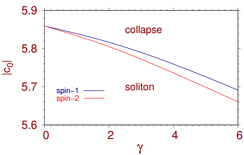
Figure 1: The $c_{0}$-$\gamma$ phase plot illustrating the collapse and soliton formation.

To obtain quasi-2D solitons with a self-attractive ($c_{0}<0$) nonmagnetic SO-coupled spin-1 BEC for different SO-coupling strengths $\gamma$, we consider a BEC with $c_{0}=-0.6$ and vary $\gamma$ in this study. We consider $c_{0}=-0.6$ because this value gives an adequate size of the soliton. A decrease in $c_{0}$ results in more attraction, hence a reduced system size, and below a critical $c_{0}=c_{0,\mathrm{crit}}$ the BEC will collapse as displayed in Fig. 1. For $\gamma=0$, the spin-1 and spin-2 systems become essentially identical and also equivalent to a scalar nonspinor BEC of $N$ atoms. The nonlinearities in the mean-field equations in these three cases are also identical. For $\gamma=0$, for a nonspinor spin-0 BEC, the critial $c_{0}$ for collapse was obtained previously as $c_{0,\mathrm{crit}}\sim-5.85$ [26, 27]. In this study we find, for spin-0, spin-1 and spin-2 cases and for $\gamma=0$, $c_{0,\mathrm{crit}}=-5.86$, quite close to this previous spin-0 result. The $c_{0,\mathrm{crit}}$ for collapse for nonzero $\gamma$ for spin-1 and spin-2 cases are slightly different as illustrated in Fig. 1. On the other hand, an increase in $c_{0}$ leads to an increased system size and, for positive (self-repulsive) values of $c_{0}$, the system is no longer self-trapped. For negative (self-attractive) values of $c_{0}$ above the critical value ($c_{0}>c_{0,\mathrm{crit}}$), the SO-coupled BEC remains self-trapped. We demonstrate in Fig. 2 how different types of solitons appear as SO-coupling strength is varied for a fixed $c_{0}$ through a phase plot of energy $\delta E\equiv(E+\gamma^{2}/2)$ against $\gamma$, where $E$ denotes the energy of the soliton and $-\gamma^{2}/2$ corresponds to the energy of single particle Hamiltonian (1) for a spin-1 BEC. We find five different types of quasi-2D solitons for different $\gamma$: (a) $(-1,0,+1)$ and $(0,+1,+2)$ multiring solitons, (b) stripe soliton with a stripe pattern in component densities only, (c) a supersolid-like soliton with component and total densities having the square-lattice pattern, and (d) asymmetric soliton. From Fig. 2, we find that for small $\gamma$ ($\gamma\lessapprox 1\sim 2$) only $(-1,0,+1)$- and $(0,+1,+2)$-type multiring solitons are possible with the $(0,+1,+2)$ soliton being an excited state. For medium $\gamma$ ($3\gtrapprox\gamma\gtrapprox 1.5)$, two new types of excited states appear: stripe and asymmetric solitons; of these the stripe soliton has a smaller energy than the asymmetric soliton. For large $\gamma$ ($\gamma\gtrapprox 3$) the square-lattice excited state appears with an energy larger than the asymmetric soliton.

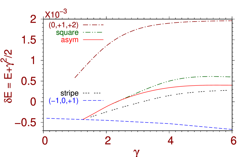
Figure 2: The $\delta E\equiv E+\gamma^{2}/2$ versus $\gamma$ phase plot for Rashba SO coupled $(-1,0,+1)$-, $(0,+1,+2)$-type multiring, asymmetric, stripe and square-lattice solitons.

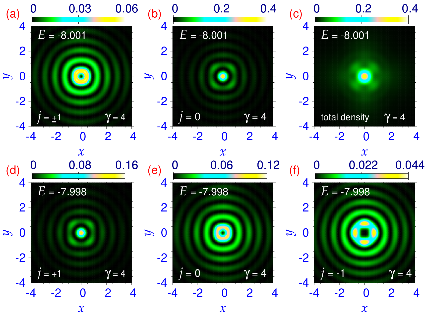
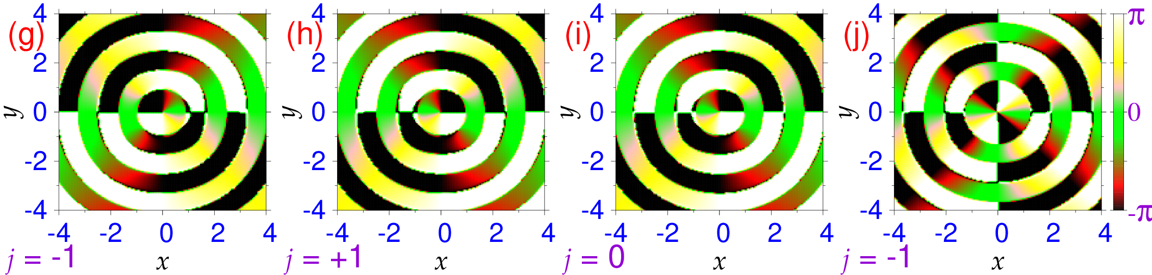
Figure 3: Top row: (a) component density $n_{\pm 1}(\boldsymbol{\rho})$, (b) $n_{0}(\boldsymbol{\rho})$, and (c) total density $n(\boldsymbol{\rho})$ of a $(-1,0,+1)$-type multiring soliton of the SO-coupled spin-1 BEC with $c_{0}=-0.6$ and $\gamma=4$. Similarly, middle row: (d) component density $n_{+1}(\boldsymbol{\rho})$, (e) $n_{0}(\boldsymbol{\rho})$, and (f) $n_{-1}(\boldsymbol{\rho})$ of a $(0,+1,+2)$-type multiring soliton of the BEC with same interaction and coupling strengths. Bottom row: phase distributions of wave-function components (g) $\psi_{+1}$, (h) $\psi_{-1}$ of the $(-1,0,+1)$-type multiring BEC soliton and those of wave-function components (i) $\psi_{0}$, (j) $\psi_{-1}$ of the $(0,+1,+2)$-type multiring BEC soliton.

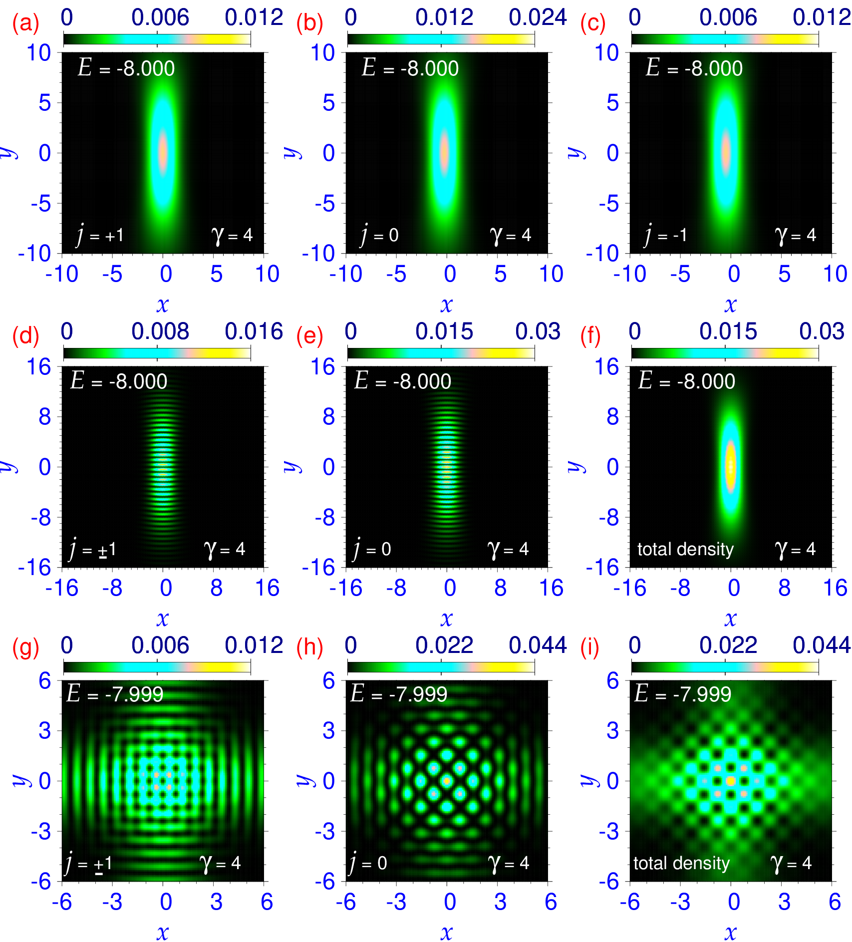
Figure 4: Top row: (a) component density $n_{+1}(\boldsymbol{\rho})$, (b) $n_{0}(\boldsymbol{\rho})$, and (c) $n_{-1}(\boldsymbol{\rho})$ of an asymmetric soliton of the SO-coupled spin-1 BEC with $c_{0}=-0.6$ and $\gamma=4$. Middle row: (d) component density $n_{\pm 1}(\boldsymbol{\rho})$, (e) $n_{0}(\boldsymbol{\rho})$, and (f) total density $n(\boldsymbol{\rho})$ of a stripe soliton and bottom row: (g) component density $n_{\pm 1}(\boldsymbol{\rho})$, (h) $n_{0}(\boldsymbol{\rho})$, and (i) total density $n(\boldsymbol{\rho})$ of a square-lattice soliton for the same interaction and coupling strengths.

For the Rashba SO coupling, we first investigate the formation of two quasi-degenerate multiring vector solitons of $(-1,0,+1)$- and $(0,+1,+2)$-type generated by solving Eqs. (3a)-(3b) in imaginary-time using initial guesses where appropriate vortices are imprinted in the components. We show the contour plots of the densities (a) $n_{\pm 1}(\boldsymbol{\rho})$, (b) $n_{0}(\boldsymbol{\rho})$, and (c) $n(\boldsymbol{\rho})$ (total density) in a $(-1,0,+1)$-type multiring soliton of the spin-1 BEC with $c_{0}=-0.6$ and $\gamma=4$ in Figs. 3(a)-(c). For the same parameters, we show the densities of three components, $n_{j}(\boldsymbol{\rho})$, in a $(0,+1,+2)$-type multiring soliton in Figs. 3(d)-(f). The energies of these $(-1,0,+1)$- and $(0,+1,+2)$-type solitons are $E=-8.001$ and $E=-7.999,$ respectively; the latter is an excited state. The phase distributions of $\psi_{+1}$ and $\psi_{-1}$ of the $(-1,0,+1)$-type multiring soliton shown in Figs. 3(g) and (h) reflect the phase shifts of $-2\pi$ and $2\pi$, respectively, under a full rotation around the center. Similarly, phase shifts by $2\pi$ and $4\pi$, respectively, under a full rotation around the center of $\psi_{0}$ and $\psi_{-1}$ of the $(0,+1,+2)$-type multiring soliton can be seen in Figs. 3(i) and (j). These phases agree with the vortex/anti-vortex structure of the $(-1,0,+1)$ and $(0,+1,+2)$-type solitons.

Besides the two circularly-symmetric solitons, asymmetric, stripe and square-lattice solitons are other stationary states of the BEC with $c_{0}=-0.6$ and $\gamma=4$. The component densities $n_{j}(\boldsymbol{\rho})$ of the asymmetric, stripe and square-lattice solitons are shown, respectively, in Figs. 4(a)-(c), 4(d)-(f), and 4(g)-(i). The energies of these three are $-8.000$, $-8.000$ and $-7.999$, respectively. The stripe soliton has a stripe pattern in the density $n_{j}(\boldsymbol{\rho})$ of each component, whereas the total density $n(\boldsymbol{\rho})$ is devoid of this pattern. The square-lattice soliton, on other hand, has a square lattice pattern in each component density $n_{j}(\boldsymbol{\rho})$ and also in the total density $n(\boldsymbol{\rho})$. The energies of the different solitons for $\gamma=4$ satisfy $E(0,+1,+2)>E$(squarelattice) $>E$(asymmetric) $>E$(stripe) $>E(-1,0,+1)$. The stripe and the square-lattice solitons are efficiently obtained in numerical calculation, if such periodic patterns are imprinted on the initial state [5]

3.2 Nonmagnetic quasi-2D solitons in an SO-coupled spin-2 BEC

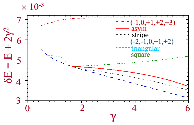
Figure 5: The $\delta E\equiv E+2\gamma^{2}$ versus $\gamma$ phase plot for Rashba SO-coupling of $(-2,-1,0,+1,+2)$- and $(-1,0,+1,+2,+3)$-type multiring, asymmetric, triangular-lattice, stripe and square-lattice solitons.

  

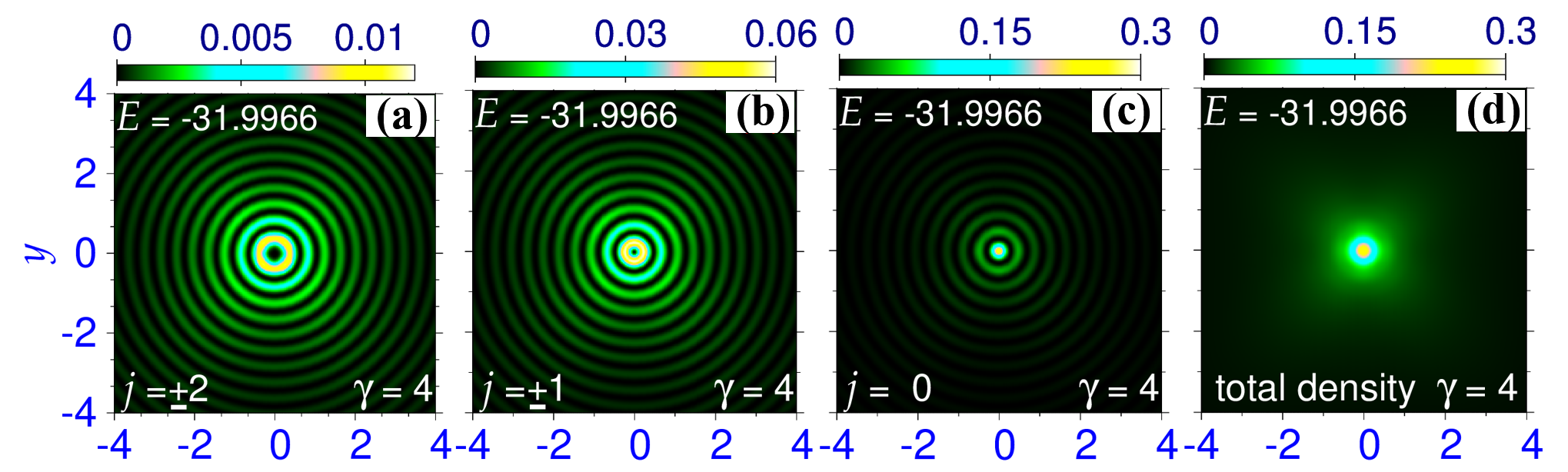
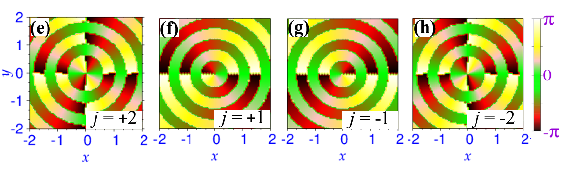
Figure 6: Upper row: (a) component density $n_{\pm 2}(\boldsymbol{\rho})$, (b) $n_{\pm 1}(\boldsymbol{\rho})$, (c) $n_{0}(\boldsymbol{\rho})$, and (d) total density $n(\boldsymbol{\rho})$ of a $(-2,-1,0,+1,+2)$-type multiring soliton of the SO-coupled spin-2 BEC with $c_{0}=-0.2$ and $\gamma=4$. Lower row: phase distributions of wave-function components (e) $\psi_{+2}$, (f) $\psi_{+1}$, (g) $\psi_{-1}$, and (h) $\psi_{-2}$ in the same soliton.

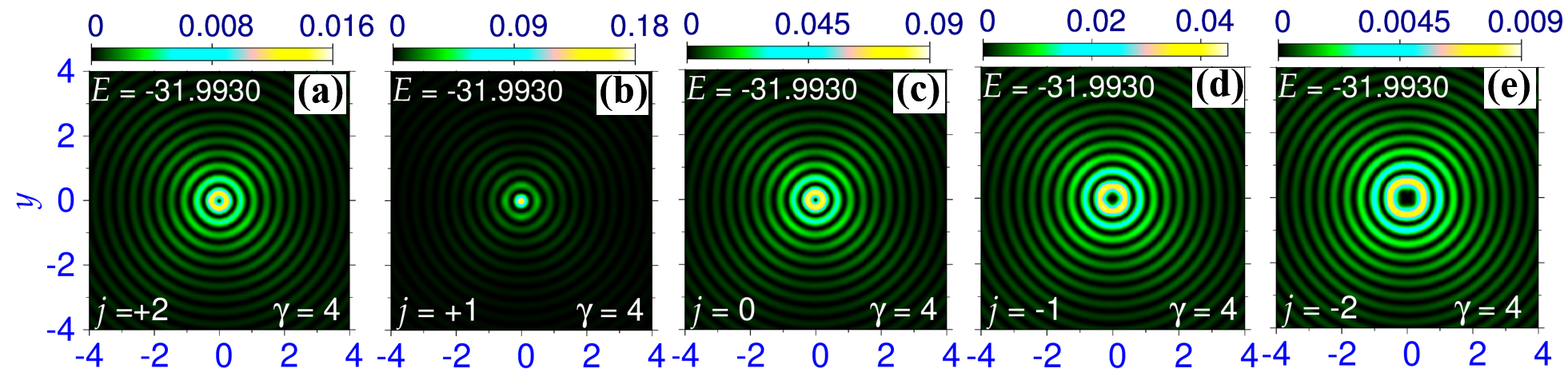
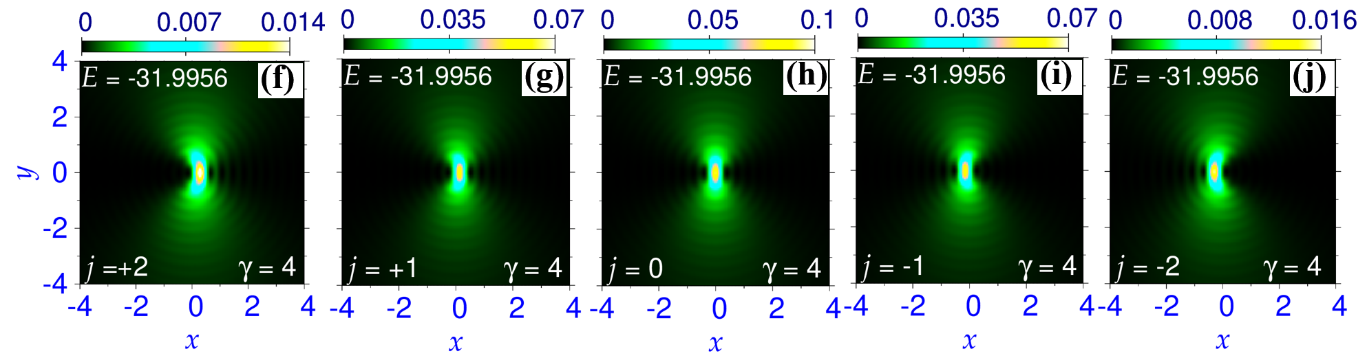
Figure 7: Upper row: (a) component density $n_{+2}(\boldsymbol{\rho})$, (b) $n_{+1}(\boldsymbol{\rho})$, (c) $n_{0}(\boldsymbol{\rho})$, (d) $n_{-1}(\boldsymbol{\rho})$, and (e) $n_{-2}(\boldsymbol{\rho})$ of a $(-1,0,+1,+2,+3)$-type multiring soliton of the SO-coupled spin-1 BEC with $c_{0}=-0.2$ and $\gamma=4$. Bottom row: (f) component density $n_{+2}(\boldsymbol{\rho})$, (g) $n_{+1}(\boldsymbol{\rho})$, (h) $n_{0}(\boldsymbol{\rho})$, (i) $n_{-1}(\boldsymbol{\rho})$, and (j) $n_{-2}(\boldsymbol{\rho})$ of an asymmetric soliton for the same interaction and coupling strengths.

Similar to a nonmagnetic SO-coupled spin-1 BEC, for a nonmagnetic SO-coupled spin-2 BEC too, several self-trapped stationary states are possible, including those in which the density $n(\boldsymbol{\rho})$ of the condensate displays spatially-periodic patterns. As in the spin-1 BEC, there are two types of multiring solitons as well as spatially-periodic stripe and square-lattice solitons. In addition, we observe a triangular-lattice soliton that was absent in the spin-1 BEC. For $f=2$, we consider $c_{0}=-0.2$. Again, for large $|c_{0}|$ the system collapses as shown in Fig. 1. Here the phase plot of $\delta E=(E+2\gamma^{2}$) versus $\gamma$ in Fig. 5 shows how different types of solitons emerge for Rashba SO coupling, where $E$ again is the energy of the soliton and $-2\gamma^{2}$ is that of the single-particle Hamiltonian (1) for a spin-2 BEC. We find six different types of quasi-2D solitons for different $\gamma$: (a) $(-2,-1,0,+1,+2)$- and $(-1,0,+1,+2,+3)$-type multiring solitons, (b) stripe soliton with stripe patterns in component densities only, (c) square-lattice soliton having square-lattice patterns in total and all component densities, (d) asymmetric soliton, and (e) triangular-lattice soliton where a triangular-lattice pattern is present in the component and total densities, similar to a supersolid. According to Fig. 5, multiring solitons of the types $(-2,-1,0,+1,+2)$ and $(-1,0,+1,+2,+3)$ are possible for small $\gamma$ ($\gamma\lessapprox 1$). For intermediate strengths of $\gamma$ ($\gamma\approx 1$), triangular-lattice solitons also appear as a quasi-degenerate state. For larger $\gamma$ ($\gamma\gtrapprox 2$), asymmetric, stripe and square-lattice solitons appear. These excited states in the spin-2 BEC appear in the same order as the corresponding states in the spin-1 case shown in Fig. 2. The only difference in the spin-2 case is the appearance of the triangular-lattice soliton which is absent in the spin-1 case.

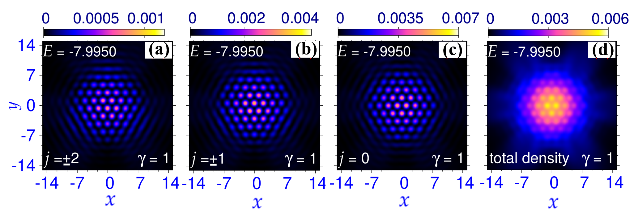
Figure 8: (a) Component density $n_{\pm 2}(\boldsymbol{\rho})$, (b) $n_{\pm 1}(\boldsymbol{\rho})$, (c) $n_{0}(\boldsymbol{\rho})$, and (d) total density $n(\boldsymbol{\rho})$ of a triangular-lattice soliton of the SO-coupled spin-2 BEC with $c_{0}=-0.2$ and $\gamma=1$.

We illustrate the formation of a $(-2,-1,0,+1,+2)$-type multiring soliton for $c_{0}=-0.2$ and $\gamma$ = 4 having energy $-31.9966$ in Figs. 6(a)-(d), where we display the contour plots of (a) component densities $n_{\pm 2}(\boldsymbol{\rho})$, (b) $n_{\pm 1}(\boldsymbol{\rho})$, (c) $n_{0}(\boldsymbol{\rho})$, and (d) total density $n(\boldsymbol{\rho})$ of this soliton. The charge of phase singularities in $\psi_{\pm 2}$ and $\psi_{\pm 1}$ are ascertained from Figs. 6(e)-(h), where we display the contour plots of the phases of wave-function components of the $(-2,-1,0,+1,+2)$-type Rashba SO-coupled soliton. The phases correspond to phase changes of $\mp 4\pi$ and $\mp 2\pi$ in $j=\pm 2$ and $j=\pm 1$ components, respectively, under a complete rotation around the center. As discussed earlier, we also have $(-1,0,+1,+2,+3)$-type multiring soliton that continues to be the solution of Eqs. (4a)-(4c) for large SO coupling strengths. In Fig. 7, we show its emergence for $c_{0}=-0.2$ and $\gamma=4$ via contour plots of densities (a) $n_{+2}(\boldsymbol{\rho})$, (b) $n_{+1}(\boldsymbol{\rho})$, (c) $n_{0}(\boldsymbol{\rho})$, (d) $n_{-1}(\boldsymbol{\rho})$, and (e) $n_{-2}(\boldsymbol{\rho})$ with energy $-31.9930$. Next in Fig. 7, we show the contour densities (f) $n_{+2}(\boldsymbol{\rho})$ , (g) $n_{+1}(\boldsymbol{\rho})$, (h) $n_{0}(\boldsymbol{\rho})$, (i) $n_{-1}(\boldsymbol{\rho})$, and (j) $n_{-1}(\boldsymbol{\rho})$ of the asymmetric soliton for $c_{0}=-0.2$ and $\gamma=4$ and with energy $-31.9956$. For an intermediate SO-coupling strength of $\gamma=1$, contour plots of (a) densities $n_{\pm 2}(\boldsymbol{\rho})$, (b) $n_{\pm 1}(\boldsymbol{\rho})$, (c) $n_{0}(\boldsymbol{\rho})$ and (d) total density $n(\boldsymbol{\rho})$ of the triangular-lattice soliton for $c_{0}=-0.2$ and with energy $-7.9950$ are shown in Figs. 8(a)-(d). This soliton has a hexagonal-lattice crystallization in component and total densities. Besides the asymmetric soliton, two other solitons, which appear explicitly for large SO-coupling strengths, are stripe and square-lattice solitons. In Fig. 9 we present the contour plots of (a) densities $n_{\pm 2}(\boldsymbol{\rho})$, (b) $n_{\pm 1}(\boldsymbol{\rho})$, (c) $n_{0}(\boldsymbol{\rho})$, and (d) total density $n(\boldsymbol{\rho})$ of the stripe soliton of energy $-31.9962$ for $c_{0}=-0.2$ and $\gamma=4$. Similar to the stripe soliton in the SO-coupled spin-1 BEC, the component densities have a stripe pattern which is not present in their sum. The scenario is different in the case of a square-lattice soliton. For example, the component and total densities of the square-lattice soliton of energy $-31.9950$ for $c_{0}=-0.2$ and $\gamma=4$ are shown in Fig. 9: (e) $n_{\pm 2}(\boldsymbol{\rho})$, (f) $n_{\pm 1}(\boldsymbol{\rho})$, (g) $n_{0}(\boldsymbol{\rho})$, and (h) total density $n(\boldsymbol{\rho})$, where the square-lattice pattern in the total density as well as the component densities is explicit.

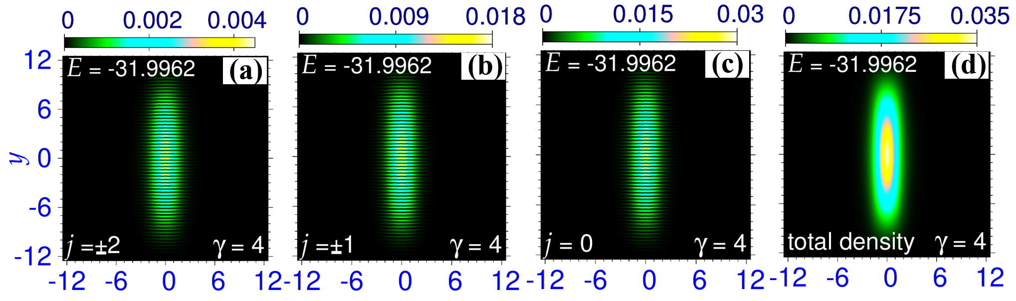
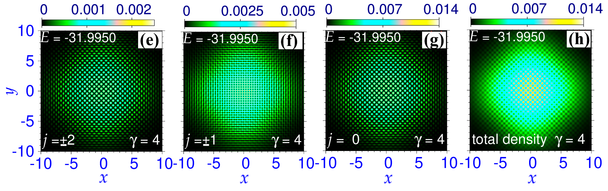
Figure 9: Upper row: (a) component density $n_{\pm 2}(\boldsymbol{\rho})$, (b) $n_{\pm 1}(\boldsymbol{\rho})$, (c) $n_{0}(\boldsymbol{\rho})$, and (d) total density $n(\boldsymbol{\rho})$ of a stripe Rashba SO-coupled soliton with $c_{0}=-0.2$ and $\gamma=4$. Lower row: (a) component density $n_{\pm 2}(\boldsymbol{\rho})$, (b) $n_{\pm 1}(\boldsymbol{\rho})$, (c) $n_{0}(\boldsymbol{\rho})$, and (d) total density $n(\boldsymbol{\rho})$ of a square-lattice soliton with the same $c_{0}$ and $\gamma$.

4 Summary of Results

We have investigated spontaneous spatial order in a Rashba SO-coupled nonmagnetic trapless quasi-2D spin-1 and spin-2 BECs for various SO-coupling strengths $\gamma$ without spinor interactions by numerically solving the coupled GP equations. For small SO coupling, $(-1,0,+1)$ and $(0,+1,+2)$-type solitons are found for a spin-1 BEC, whereas $(-2,-1,0,+1,+2)$ and $(-1,0,+1,+2,+3)$-type solitons are found for a spin-2 BEC, which develop multiring structure with an increase in SO coupling strengths. For intermediate strengths of SO-coupling ($\gamma\approx 1$), in spin-2 BEC, triangular-lattice soliton having hexagonal crystallization in component as well as total density appears as quasi-degenerate state. For relatively larger SO-coupling strengths, asymmetric, stripe and square-lattice solitons appear as quasi-degenerate solitons for spin-1 and spin-2 BECs. We also established the dynamical stability of these solitonic states by stable real-time simulation over a long interval of time as in the case of spin-1 and spin-2 ferromagnetic, anti-ferromagnetic and cyclic solitons [5, 7] (result not shown here). The spatially-periodic structures are not possible in multicomponent BECs with only the contact interaction present. The presence of the SO-coupling terms with first derivatives, mixing the components, are the necessary ingredients for the emergence of different types of spatially-periodic solitons. In conclusion, it is strongly suggestive that the spatially-periodic supersolid-like states found in SO-coupled pseudo spin-1/2 [1, 3, 4], spin-1 [5], and spin-2 [7] spinor BECs are not a consequence of spinor interactions but are a consequence of multicomponent nature of these states in presence of SO coupling.

References

- [1] J.-R. Li, J. Lee, W. Huang, S. Burchesky, B. Shteynas, F. Ç. Top, A. O. Jamison, W. Ketterle, Nature 543 (2017) 91.
- [2] A. Putra, F. Salces-Cárcoba, Y. Yue, S. Sugawa, I. B. Spielman, Phys. Rev. Lett. 124 (2020) 053605.
- [3] Y. Li, G. I. Martone, L. P. Pitaevskii, S. Stringari, Phys. Rev. Lett. 110 (2013) 235302.
- [4] S. K. Adhikari, J. Phys.: Condens. Matter 33 (2021) 425402.
- [5] S. K. Adhikari, Phys. Rev. A 103 (2021) L011301; S. K. Adhikari, Phys. Lett. A 388 (2021) 127042.
- [6] S. K. Adhikari, J. Phys.: Condens. Matter 33 (2021) 265402.
- [7] P. Kaur, S. Gautam, S. K. Adhikari, Phys. Rev. A 105 (2022) 023303.
- [8] Y. Kawaguchi, M. Ueda, Phys. Rep. 520 (2012) 253; D. M. Stamper-Kurn, M. Ueda, Rev. Mod. Phys. 85 (2013) 1191.
- [9] J. Stenger, S. Inouye, D. M. Stamper-Kurn, H.-J. Miesner, A. P. Chikkatur, W. Ketterle, Nature 396 (1998) 345.
- [10] V. I. Yukalov, Laser Phys. 28 (2018) 053001; S. Gautam, S. K. Adhikari, Phys. Rev. A 92 (2015) 023616; Y. Kawaguchi, M. Ueda, Phys. Rep. 520 (2012) 253.
- [11] C. V. Ciobanu, S.-K. Yip, T.-L. Ho, Phys. Rev. A 61 (2000) 033607.
- [12] A. Widera, F. Gerbier, S. Folling, T. Gericke, O. Mandel, I. Bloch, New J. Phys. 8 (2006) 152.
- [13] S. Inouye, M. R. Andrews, J. Stenger, H.-J. Miesner, D. M. Stamper-Kurn, W. Ketterle, Nature 392 (1998) 151.
- [14] T. Mizushima, K. Machida, T. Kita, Phys. Rev. Lett. 89 (2002) 030401; T. Mizushima, K. Machida, T. Kita, Phys. Rev. A 66 (2002) 053610.
- [15] P.-K. Chen, L.-R. Liu, M.-J. Tsai, N.-C. Chiu, Y. Kawaguchi, S.-K. Yip, M.-S. Chang, Y.-J. Lin, Phys. Rev. Lett. 121 (2018) 250401.
- [16] A. F. Andreev, I. M. Lifshitz, Zurn. Eksp. Teor. Fiz. 56 (1969) 2057 [English Transla.: Sov. Phys. JETP 29 (1969) 1107]; E. P. Gross, Phys. Rev. 106 (1957) 161; A. J. Leggett, Phys. Rev. Lett. 25 (1970) 1543; G. V. Chester, Phys. Rev. A 2 (1970) 256; V. I. Yukalov, Phys. 2 (2020) 49.
- [17] M. H. Anderson, J. R. Ensher, M. R. Matthews, C. E. Wieman, E. A. Cornel, Science 269 (1995) 198; K. B. Davis, M.-O. Mewes, M. R. Andrews, N. J. van Druten, D. S. Durfee, D. M. Kurn, W. Ketterle, Phys. Rev. Lett. 75 (1995) 3969.
- [18] M. W. Zwierlein, C. H. Schunck, A. Schirotzek, W. Ketterle, Nature 442 (2006) 54; M. Greiner, C. A. Regal, D. S. Jin, Nature 426 (2003) 537.
- [19] F. Böttcher, J.-N. Schmidt, M. Wenzel, J. Hertkorn, M.Guo, T. Langen, T. Pfau, Phys. Rev. X 9 (2019) 011051; L. Chomaz, D. Petter, P. Ilzhöfer, G. Natale, A. Trautmann, C. Politi, G. Durastante, R. M. W. van Bijnen, A. Patscheider, M. Sohmen, M. J. Mark, F. Ferlaino, Phys. Rev. X 9 (2019) 021012; L. Tanzi, E. Lucioni, F. Famá, J. Catani, A. Fioretti, C. Gabbanini, R. N. Bisset, L. Santos, G. Modugno, Phys. Rev. Lett. 122 (2019) 130405.
- [20] G. Natale, R. M. W. van Bijnen, A. Patscheider, D. Petter, M. J. Mark, L. Chomaz, F. Ferlaino, Phys. Rev. Lett. 123 (2019) 050402; L. Tanzi, S. M. Roccuzzo, E. Lucioni, F. Famà, A. Fioretti, C. Gabbanini, G. Modugno, A. Recati, S. Stringari, Nature 574 (2019) 382; M. Guo, Fabian Böttcher, J. Hertkorn, J.-N. Schmidt, M. Wenzel, H. P. Büchler, T. Langen, T. Pfau, Nature 574 (2019) 386; J. Hertkorn, F. Böttcher, M. Guo, J. N. Schmidt, T. Langen, H. P. Büchler, T. Pfau, Phys. Rev. Lett. 123 (2019) 193002.
- [21] L. Salasnich, A. Parola, L. Reatto, Phys. Rev. A 65 (2002) 043614.
- [22] Y.-J. Lin, K. Jiménez-García, I. B. Spielman, Nature 471 (2011) 83.
- [23] P. Muruganandam, S. K. Adhikari, Comput. Phys. Commun. 180 (2009) 1888; D. Vudragović, I. Vidanović, A. Balaž, P. Muruganandam, S. K. Adhikari, Comput. Phys. Commun. 183 (2012) 2021; L. E. Young-S., D. Vudragović, P. Muruganandam, S. K. Adhikari, A. Balaž, Comput. Phys. Commun. 204 (2016) 209; L. E. Young-S., P. Muruganandam, S. K. Adhikari, V. Lončar, D. Vudragović, Antun Balaž, Comput. Phys. Commun. 220 (2017) 503.
- [24] P. Banger, P. Kaur, S. Gautam, Int. J. Mod. Phys. C 33(04) (2022) 2250046; P. Kaur, A. Roy, S. Gautam, Comput. Phys. Commun. 259 (2021) 107671; P. Banger, P. Kaur, A. Roy, S. Gautam, Comput. Phys. Commun. 279 (2022) 108442.
- [25] R. Ravisankar, D. Vudragović, P. Muruganandam, A. Balaž, S. K. Adhikari, Comput. Phys. Commun. 259 (2021) 107657;
- [26] H. Sakaguchi, B. A. Malomed, Phys. Rev. E 73 (2006) 026601.
- [27] B. Bakkali-Hassani, C. Maury, Y.-Q. Zou, É. Le Cerf, R. Saint-Jalm, P. C. M. Castilho, S. Nascimbene, J. Dalibard, J. Beugnon, Phys. Rev. Lett. 127 (2021) 023603.