A Category of Surface-Embedded Graphs

Abstract

We introduce a categorical formalism for rewriting surface-embedded graphs. Such graphs can represent string diagrams in a non-symmetric setting where we guarantee that the wires do not intersect each other. The main technical novelty is a new formulation of double pushout rewriting on graphs which explicitly records the boundary of the rewrite. Using this boundary structure we can augment these graphs with a rotation system, allowing the surface topology to be incorporated.

1 Introduction

String diagrams [18] are a graphical formalism to reason about monoidal categories. Equational reasoning in symmetric string diagrams can be implemented as graph or hyper-graph rewriting subject to various side conditions to capture the precise flavour of the monoidal category intended [6, 7, 8, 15, 3, 2]. We want to use string diagrammatic reasoning for monoidal categories which are not necessarily symmetric. Informally, the lack of symmetry is often stated as “the wires cannot cross” – but what does that mean when the string diagram is a graph or other combinatorial object? Where is this “crossing” taking place? To make sense of this we must move beyond the situation where only the connectivity matters and add some topological information.

In this paper we make two steps in that direction. Firstly we borrow a tool from topological graph theory – rotation systems – and use it to define a category of graphs which are embedded in some surface. Secondly, we introduce a new refinement of double pushout rewriting [10] which is adapted to this category. This refinement was motivated by the desire to do rewriting on rotation systems, however it works on conventional directed graphs equally well, and removes many annoyances encountered when using standard techniques from algebraic graph rewriting in string diagrams. This is an important step towards formalising non-symmetric string diagrams and their rewriting theory.

Our motivation is also twofold. From the abstract point of view, non-symmetric string diagrams can capture a larger class of theories, including both the symmetric case and the braided monoidal one. A more practical motivation comes from the area of quantum computing, where string diagrams are often used to model quantum circuits [4], their connectivity restrictions imposed by the qubit architecture [5] require a theory without implicit SWAP gates, and can involve circuits defined on quite complex surfaces.

Curiously, Joyal and Street’s original work [13] formalised monoidal categories as plane embedded diagrams, and used the plane to carry the categorical structure. Our work goes in the opposite direction: to recover the topology from the combinatorial structure.

Graph Embeddings

Graphs can be drawn on surfaces, and the same graph be drawn different ways on the same surface, as shown below.

If, like the one on the right, the drawing does not intersect itself then it defines an embedding of the graph into the surface. If a graph can be embedded in the plane (or equivalently surface of the sphere) it is called planar. However in this work we will be concerned with graphs with a given embedding into some closed compact surface, which need not be the plane.

Dealing with lines and points as submanifolds of some surface (up to homeomorphism) is quite unwieldy, so we use a combinatorial representation of graph embeddings called rotation systems. A rotation system imposes an order on the edges incident at vertex (called a rotation). The rotation information at each vertex is enough to fix the embedding of the graph into some surface, as it defines the faces of the embedding uniquely. This is a well studied topic in graph theory and we refer to the literature for more details [11].

Theorem 1.1.

A rotation system determines the embedding of a connected graph into a minimal surface up to homeomorphism [12, 9, 11].

Note that different rotation systems for the same graph may have different minimal surfaces, which need not be the plane.

Boundary Graphs and Partitioning Spans

When using string diagrams, graphs as usually defined are not the most natural object; rather, we often think about open graphs which have “half-edges” or “dangling wires” which represent the domain and codomain of the morphism in question. The half-edges therefore provide the interface along which morphisms compose, and also where substitutions can be made in rewriting. Unfortunately half-edges don’t work particularly well with double pushout rewriting, necessitating various workarounds encoding the “wires” as special vertices in a graph [8] or hypergraph [2]. This in turn leads to its own complications when we consider the identity morphism, and other natural transformations which are naturally “all string”; equations which should be trivial are no longer so. Surface embedded graphs suggest a different approach to this question.

Naively, when picturing a rewrite on a surface embedded graph, we picture a disc-like region of the surface which is removed and replaced. The edges which cross the boundary of this region define the interface and we naturally require that the removed disc and its replacement should have the same interface. From the outside, this disc is homeomorphic to a point, so it can be treated as if it was a vertex equipped with a rotation system. However, the perspective from inside and outside the region are completely equivalent, so we can dually view the rest of the graph as a single vertex connected to the interior of the disc. We think of and draw a graph with boundary in three different ways:

On the left, the graph is depicted as a region of the surface with its outside being the rest of the surface. In the middle, graph and its surrounding are both regions of the surface, and on the right we have drawn the boundary as a vertex with the interconnecting edges attached.

This leads naturally to our notion of boundary graph: we contract both subgraphs on either side of the boundary to points, leaving a two-vertex graph whose edges specify the connections crossing the boundary. Boundary graphs form the vertex of partitioning spans, which specify the whole graph as the two parts, as shown in Figure 1; the pushout of a partitioning span is the original graph.

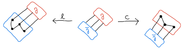
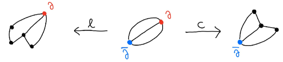
Figure 1: Example of a partitioning span, drawn in a region- and a vertex-style (edge directions are omitted for readability)

This formalism allow us to use a simple definition of graph, although our morphisms are now built from partial functions, which introduces some complications around the required injectivity properties to preserve the type of the vertices, which is essential if these graphs are to be interpreted as string diagrams.

Limitations

The astute reader will have noted that Theorem 1.1 applies only to connected graphs. To specify an embedding of a disconnected graph a rotation system does not suffice. We would also need to take into account the relationship between components and faces of the graph. We have made no attempt to do so here.

2 A Suitable Category of Graphs

In this section we will introduce a category of directed graphs without reference to any topological structure. The main difficulty here is arriving at the correct notion of graph morphism: our intent here is that the graphs represent terms in some monoidal category – i.e. string diagrams – and the morphisms represent embeddings of subterms. This implies that certain structures should be preserved which conventional graph rewriting does not worry about. Our choices here are also influenced by the variant of double-pushout rewriting we will define in the next section. In later sections we will show how to incorporate the plane topology by adding rotation systems.

A total graph is a functor $G:(\bullet\rightrightarrows\bullet)\ \to\ \mathbf{Set}$. Concretely, such a graph is a pair of sets $V$ and $E$, of vertices and edges respectively, and a pair of functions $s$ and $t$ assigning source and target vertices to each edge.

In the functor category $[\bullet\rightrightarrows\bullet,\mathbf{Set}]$, a morphism of graphs is a pair of functions $f_{V}:V\rightarrow V^{\prime},f_{E}:E\rightarrow E^{\prime}$, such that the following squares commute:

             (1)

Sadly for us, this simple and elegant definition will not suffice.

We want to consider graph morphisms which can replace vertices with subgraphs, and therefore forget these vertices, as shown below:

To achieve this we could operate in a subcategory of $[\bullet\rightrightarrows\bullet,\mathbf{Pfn}]$, the category of partial graphs and maps, with only the total graphs as objects. However this is not quite enough. Commutation of the naturality squares (1) in this category is strict, meaning it includes equality of the domains of definition. Therefore if a morphism forgets a vertex it must also forget all the incident edges at that vertex. This is no use. We address this issue by using the poset enrichment of $\mathbf{Pfn}$, and work in the category $[\bullet\rightrightarrows\bullet,\mathbf{Pfn}]_{\leq}$ of functors and lax natural transformations:

             (2)

The lax commutation allows the vertex component of a morphism to be undefined at some vertex $v$ while its incident edges may be preserved. However, if an edge is “forgotten” then its source and target vertices must also be so. We’ll need more, but let’s take $[\bullet\rightrightarrows\bullet,\mathbf{Pfn}]_{\leq}$ as our ambient category for now.

Proposition 2.1.

The category $\mathbf{Pfn}$ of sets and partial functions has pushouts.

Proof.

Given a span , the elements of the pushout are the same as in for $\mathbf{Set}$, but restricted to a subset $B^{\prime}\subseteq B$, with both $l(b)$ and $c(b)$ defined for $b\in B^{\prime}$. This is the only way the square commutes for elements in $B^{\prime}$, and the universal property of the pushout can be derived from $\mathbf{Set}$. ∎

Proposition 2.2.

The category $\mathbf{Inj}$ of sets and injective functions does not have pushouts.

Proof.

If pushouts in $\mathbf{Inj}$ exist, they have to coincide with those of $\mathbf{Set}$. Consider the span , and commuting squares:

In the square all morphisms are injective, but the mediating map out of the pushout $m:\{\ast,\ast\}\rightarrow\{\ast\}$ is not. ∎

We would like to be able to accommodate two further properties in our notion of graph morphism: Firstly, since vertices represent morphisms of a monoidal category, their type should be preserved. Secondly, we want to specify when a morphism is a graph embedding, which requires an injectivity property. Merely asking for injectivity of the vertex and edge component is not enough though, our setup requires the edge component to be non-injective, i.e. to represent the identity morphism (or similar circumstances):

Example 2.3.

A graph morphism with a non-injective edge component:

Both of the above requirements turn out to be properties of the connection points between vertices and their incident edges, called flags:

Definition 2.4.

Given a graph $(V,E,s,t)$ its set of flags is defined

$$F=\{(e,s(e)):e\in E\}+\{(e,t(e)):e\in E\}$$

Given a graph morphism $f:G\to G^{\prime}$ there is an induced flag map, $f_{F}:F\to F^{\prime}$,

$$f_{F}=(f_{E}\times f_{V})+(f_{E}\times f_{V})$$

Note that the flag map is in general a partial map: it is undefined on $(e,v)$, whenever $f_{V}$ is undefined on $v$. Whenever $f_{F}$ is injective we say that $f$ is flag injective.

Flag injectivity allows edges to be combined but prevents a morphism from decreasing a vertex degree in the process. However, nothing said so far forbids a morphism from increasing the degree of a vertex: we require a notion of flag surjectivity. Given $f:G\to G^{\prime}$, it doesn’t suffice to require the flag map $f_{F}$ to be surjective, since in general $G^{\prime}$ will contain more vertices than $G$, and hence more flags. The resulting definition is unfortunately unintuitive.

Definition 2.5.

Let $f:G\to G^{\prime}$ be a morphism between two total graphs; we say that $f$ is flag surjective if the two diagrams below commute laxly,

             (3)

where $s^{-1}$ and $t^{-1}$ are the preimage maps of $s$ and $t$ respectively, and $P$ is the powerset functor.

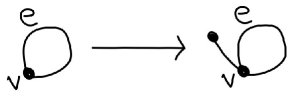
Figure 9: This map is not flag surjective and therefore not a valid morphism in $\mathcal{G}$.

If a flag surjective morphism $f$ is defined on a vertex $v$, it will ensure that all edges attached to $v^{\prime}=f_{V}(v)$ are in the image of $f_{E}$, thus no additional edges can be attached to $v^{\prime}$ in the process. An example of a morphism which is not flag surjective can be found in Figure 9 in Appendix B.
We’ll call a morphism which is both flag injective and flag surjective a flag bijection. This is quite a strong property; it’s almost enough to make the vertex map injective, but not quite.

Lemma 2.6.

Let $f:G\to G^{\prime}$ be a flag bijection, and suppose that $f_{V}(v_{1})=f_{V}(v_{2})$ and both are defined; then $\deg{v_{1}}=\deg{v_{2}}=0$.

Proof.

Let $v^{\prime}=f_{V}(v_{1})=f_{V}(v_{2})$; since $f$ is flag injective, the set of flags at $v^{\prime}$ must contain (the image of) the disjoint union of the flags at $v_{1}$ and $v_{2}$; hence $\deg{v^{\prime}}\geq\deg{v_{1}}+\deg{v_{2}}$. Since (by (2)) $f_{E}$ is defined on all the flags at $v_{1}$, flag surjectivity implies that $\deg{v_{1}}\geq\deg{v^{\prime}}$, and similarly for $v_{2}$. Hence $\deg{v^{\prime}}=\deg{v_{1}}=\deg{v_{2}}=0$. ∎

Lemma 2.7.

Let $G$ and $G^{\prime}$ be total graphs, and let $f:G\to G^{\prime}$ be a flag bijection. For all $v\in V$, if $f_{V}(v)$ is defined, then $f_{E}$ defines a bijection between the flags at $v$ and those incident at $f_{V}(v)$; in consequence $\deg v=\deg{f_{V}(v)}$.

Proof.

Let $v^{\prime}=f_{V}(v)$. The edges incident at $v$ are given by the disjoint union of $s^{-1}(v)$ and $t^{-1}(v)$, and likewise at $v^{\prime}$. Since $f$ is flag injective, $f_{E}$ is injective on the subset of flags defined by $v$. Since $f$ is flag surjective all the flags at $v^{\prime}$ are in the image of $f_{E}(s^{-1}(v))+f_{E}(t^{-1}(v))$. Note that since $f_{V}(v)$ is defined then $f_{E}$ is defined for all $e\in s^{-1}(v)$ and all $e\in t^{-1}(v)$ by Eq. (2). Hence we have a bijection as required. ∎

Lemma 2.8.

Let $f:G\to H$ and $g:H\to J$ be flag bijections; then $g\circ f$ is a flag bijection.

Proof.

See Appendix A. ∎

By the preceding lemma, and by observing that the identity is a flag bijection, we may conclude that the flag bijections define a wide subcategory of $[\bullet\rightrightarrows\bullet,\mathbf{Pfn}]_{\leq}$, which we will call $\mathcal{B}$.

Example 2.3 suggests a confounding special case: the vertex of a self loop can be forgotten. Here is another one:

Example 2.9.

Let $G$ be the (unique) total graph with one vertex and one edge; let $G^{\prime}$ be the (unique) partial graph with no vertices and a single edge. Define $f:G\to G^{\prime}$ by $f_{V}=\emptyset$ and $f_{E}=\mathrm{id}_{\mathbf{1}}$. This is a valid flag bijection in $\mathcal{B}$.

While it is tempting to restrict to the subcategory defined by the total graphs, and ban such monsters by fiat, they do occur quite naturally in the rewrite theory we propose, albeit in quite restricted circumstances. So they must be tamed. To do so, we extend the definition of graph with circles: closed edges which have neither a source nor a target vertex. Unfortunately the definition of graph morphism will get more complex and the resulting category is no longer a functor category, as we shall now see.

Definition 2.10.

A graph with circles is a 5-tuple $G=(V,E,O,s,t)$ where $(V,E,s,t)$ is a total graph and $O$ is a set of circles. For notational convenience we define the set of arcs as the disjoint union $A=E+O$.

A morphism $f:G\to G^{\prime}$ between two graphs with circles consists of two (partial) functions $f_{V}:V\rightharpoonup V^{\prime}$ as above, and $f_{A}:A\to A^{\prime}$, satisfying the conditions listed below. Note that any such $f_{A}$ factors as four maps,

$$\begin{array}[]{ccc}f_{E}:E\to E^{\prime}&&f_{EO}:E\to O^{\prime}\\ f_{OE}:O\to E^{\prime}&&f_{O}:O\to O^{\prime}\\ \end{array}$$

The following conditions must be satisfied:

1. $f_{A}:A\to A^{\prime}$ is total;

2. the component $f_{OE}:O\to E^{\prime}$ is the empty function;

3. the pair $(f_{V},f_{E})$ forms a flag surjection between the underlying graphs in $\mathcal{B}$.

If, additionally, the following three conditions are satisfied, we call the morphism an embedding:

1. $f_{V}:V\rightharpoonup V^{\prime}$ is injective;

2. the component $f_{O}$ is injective;

3. the pair $(f_{V},f_{E})$ forms a flag bijection between the underlying graphs.

It’s worth noticing that if some $f_{A}$ maps an edge $e$ to a circle, then $f_{E}(e)$ is undefined, but $f_{EO}(e)$ is defined. This, by the lax naturality property, implies that $f_{V}$ is undefined on both $s(e)$ and $t(e)$. Various examples and non-examples of morphisms and embeddings of graphs with circles can be found in Appendix B.

Lemma 2.11.

Defining composition point-wise, the composite of two morphisms of graphs with circles is again such a morphism. Additionally, if both morphisms are embeddings, their composition is an embedding as well.

Proof.

See Appendix A. ∎

We finally have introduced all the necessary structure to define our suitable category of graphs.

Definition 2.12.

Let $\mathcal{G}$ be the category whose objects are graphs with circles, and whose arrows are morphisms as per Definition 2.10.

There is an obvious and close relationship between $\mathcal{G}$ and the category of partial graphs and flag bijections, $\mathcal{B}$. We can make this precise.

Definition 2.13.

We define a forgetful functor $U:\mathcal{G}\to\mathcal{B}$ by

Example 2.14.

Returning to Example 2.9, we see how this degenerate case fits in to the framework. We start with $G$, the unique total graph with a single vertex and a single edge (and no circles). There a single valid way to erase the vertex in $\mathcal{G}$.

Firstly observe that $G^{\prime}=(\emptyset,\{e\},\emptyset,\emptyset,\emptyset)$ as in the earlier example is not an object in $\mathcal{G}$. However $G^{\prime\prime}=(\emptyset,\emptyset,\{e\},\emptyset,\emptyset)$ is a valid graph, and the map $f:G\to G^{\prime\prime}$ which is undefined on the vertex and sends the edge to the circle is a valid morphism, indeed the only one.

Finally observe that the image of $UG^{\prime\prime}$ is the empty graph and $Uf$ is the empty function.

The term “graph with circles” is unacceptably cumbersome, so henceforth we will simply say “graph” and refer to $\mathcal{G}$ as the category of graphs. In practice the circles are rarely important, although we will devote a disappointingly large amount of this paper to them.

3 DPO Rewriting in the Suitable Category

Double pushout rewriting [10] is an approach to formalising equational theories over graphs by rewriting. Each equation is formalised as a rewrite rule $L\Rightarrow R$, and the substitution $G[R/L]$ is computed via a double pushout as shown below.

The upper span embeds a boundary graph $B$ into both $L$ and $R$; ensures that both graphs have the same connectivity, and hence that $R$ can validly replace $L$. The map $m:L\rightarrow G$ is the match, an embedding of $L$ into $G$, which shows where the rewrite will occur. The first pushout square is completed by $C$, the context graph; it is basically $G$ with $L$ removed. In the DPO approach, $C$ is computed as a pushout complement. Finally the graph $H=G[R/L]$ is the graph resulting from performing the rewrite $L\Rightarrow R$ in $G$; it is computed as a pushout.

In the algebraic graph literature the notion of adhesive category [16, 17] is commonly used, as DPO rewriting behaves well in such categories. However, adhesivity is not suitable for our purposes, since the monomorphisms of $\mathcal{G}$ don’t play any special role in our formalism. We will instead consider a specific case of maps in the DPO diagram only, and in that context show the existence of pushouts and the existence and uniqueness of pushout complements, which are similar properties to those of an adhesive categories. The key to this approach is to recognise that $B$ and $C$ are in some sense partial graphs, as to a lesser extent are $L$ and $R$; our handling of this partiality is one of the main novelties of this paper.

Notation 3.1.

Almost every map in this section is an embedding of a small object into a larger one. Wherever unambiguous to do so, we will treat these embeddings as actual inclusions so, for example, we may write $m_{E}(e)=e$ despite the fact that the domain and codomain of the map are different graphs.

In our approach the graphs $L$ and $R$ that make up a rewrite rule have an additional distinguished vertex, the boundary vertex $\partial$, which represents the rest of the world, from the perspective of $L$ (or $R$). The incident edges at $\partial$ represent the interface between $L$ and the rest of the graph it occurs in. The context graph $C$ also has a distinguished vertex, the dual boundary $\bar{\partial}$ which represents its interface. In our formalism, the graph $B$ in the middle exists only to say that these interfaces must be compatible.

Definition 3.2.

A boundary graph is a graph with exactly two vertices, $\partial$ and $\bar{\partial}$ (called respectively the boundary and dual boundary vertices), where $s(e)\neq t(e)$ for all its edges $e$, and there are no circles.

Definition 3.3.

A partitioning span is a span in $\mathcal{G}$, where $B$ is a boundary graph, the vertex component $l_{V}$ is defined on $\partial$ and undefined on $\bar{\partial}$ and, dually, $c_{V}$ is undefined on $\partial$ and defined on $\bar{\partial}$. Further, we require $l$ and $c$ to be embeddings.

An example of a partitioning span and its pushout in $\mathcal{G}$ is depicted in Figure 2. The name partitioning span arises from the fact that each of the maps out of the boundary graph replaces one half of it. Hence each graph has two regions, connected via the edges present in the boundary graph.

Figure 2: Pushout of the partitioning span from Figure 1, drawn in two different ways

Lemma 3.4.

Let be a partitioning span and suppose that $e=l_{E}(e_{1})=l_{E}(e_{2})$ in $L$ for distinct $e_{1}$ and $e_{2}$ in $E_{B}$. Then $e$ is a self-loop at $\partial$ in $L$ and for all other $e_{3}\neq e_{1}\neq e_{2}$ we have $e\neq l_{E}(e_{3})$. The same holds mutatis mutandis for $C$.

Proof.

By flag bijectivity all the flags at $\partial$ must be preserved, including distinct flags for $l_{E}(e_{1})$ and $l_{E}(e_{2})$. By hypothesis these two edges are identified so necessarily $s_{B}(e_{1})=\partial$ and $s_{B}(e_{2})=\bar{\partial}$ or vice versa. Hence $e$ is a self loop. Suppose further that $l_{E}(e_{3})=e$; then $l$ is not flag bijective, which is a contradiction. ∎

Self-loops in partitioning spans indicate that the boundary is connected back to itself without an intervening vertex. This is responsible for the failure of injectivity on edges and gives rise to degeneracy when constructing pushouts. We can study them using a dual perspective.

Definition 3.5.

The pairing graph for a partitioning span is a labelled directed graph whose vertices are $E_{B}$; each vertex receives a polarity: $+$ if $s_{B}(e)=\partial$, $-$ if $s_{B}(e)=\bar{\partial}$. We draw a blue edge between $e_{1}$ and $e_{2}$ if $l_{E}(e_{1})=l_{E}(e_{2})$ i.e. if $e_{1}$ and $e_{2}$ form self-loop in $L$; similarly we draw a red edge between $e_{1}$ and $e_{2}$ if they form a self-loop in $C$. Blue edges are directed from positive to negative polarity; red edges the reverse.

An example of a pairing graph is shown in Figure 3. The pairing graph is always bipartite: it’s immediate from the definition that vertices of the same polarity are never connected. Further, due to Lemma 3.4, each vertex can have a maximum of one edge of each colour incident to it. In consequence every connected component is just a path, possibly of length zero, possibly a cycle. From these properties, we have the following immediate corollary.

Corollary 3.6.

Let ${\cal P}$ be the pairing graph of the partitioning span ; then each connected component $p$ of ${\cal P}$ determines an edge-disjoint path on $B$. For those components which are not cycles, if the first vertex of $p$ is positive, then the path starts at $\partial$; if negative the path starts at $\bar{\partial}$. Conversely, if the last vertex of $p$ is positive, the path ends at $\bar{\partial}$ and vice versa.

The reader may already suspect that when we form the pushout of a partitioning span, the components of the pairing graph determine which edges in $B$ will be identified. This is indeed the case; it forms an intermediate result (Lemma A.3) in the proof of the next theorem.

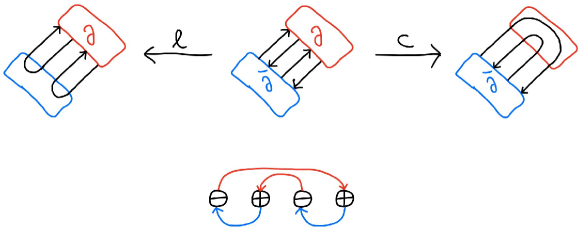
Figure 3: Example of a partitioning span with its pairing graph

Theorem 3.7.

In $\mathcal{G}$, pushouts of partitioning spans exist. Further, the maps into the pushout are embeddings.

Proof.

See Appendix A. ∎

Since pushouts of partitioning spans are the basis of the rewrite theory we wish to pursue, for the rest of the paper the term “pushout” should be understood to imply “of partitioning span”.

We now move on to the other required ingredient for DPO rewriting: pushout complements. Just as we did with partitioning spans and pushouts, we will introduce a specific kind of embedding for which the complement must exist.

Definition 3.8.

A boundary embedding is a pair of maps in $\mathcal{G}$, where $B$ is a boundary graph, where : (i) $l_{V}(\partial)$ is defined but $l_{V}(\bar{\partial})$ is undefined; and (ii) $(m_{V}\circ l_{V})(\partial)$ is undefined. Further, $L$ has to be a connected graph, and $m$ an embedding.

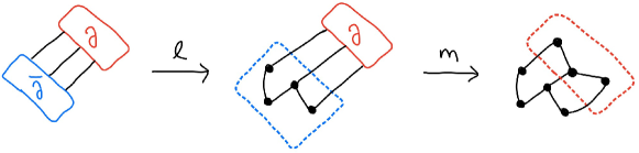
Figure 4: Example of a boundary embedding

Definition 3.9.

Given a boundary embedding we can immediately construct half a pairing graph ${\cal P}$, consisting of only the blue edges using the mapping $l:B\to L$. The re-pairing problem is to construct the other half (the red edges) so that the connected components map to the edges of $G$ (cf. Lemma A.3). See Figure 5 for examples.

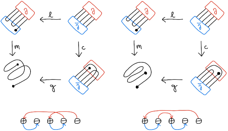
Figure 5: Two different solutions to the same re-pairing problem, together with the corresponding pairing graphs.

Lemma 3.10.

Given a boundary embedding a solution to the re-pairing problem always exists, but it is not necessarily unique.

Proof.

See Appendix A. ∎

Theorem 3.11.

In $\mathcal{G}$, pushout complements of boundary embeddings exist, and give rise to partitioning spans.

Proof.

We’ll use the boundary embedding to construct the complement $C$ such that is a partitioning span, and show that $G$ is indeed the pushout of this span.

Let $C$ have vertex set $V_{C}=(V_{G}\setminus V_{L})+\{\bar{\partial}\}$. We’ll construct the edge set, and the source and target maps, in three steps.

1. Let $E_{C}$ contain all the edges of the induced subgraph of $G$ defined by the vertices $V_{C}$, and define the source and target maps on those edges correspondingly.

2. Let $O_{C}$ contain $O_{G}\setminus m_{O}^{-1}(O_{G})$.

3. Finally we add the edges between $\bar{\partial}$ and the rest of the graph, and simultaneously define the map $c:B\to C$. Let ${\cal P}$ be a solution to the re-pairing problem given by . If in ${\cal P}$ there is a red edge between $e_{1}$ and $e_{2}$ in create a self-loop $e$ at $\bar{\partial}$ and set $c(e_{1})=c(e_{2})=e$. If there is any vertex $e$ in ${\cal P}$ which has no incident red edge, add $e$ to $E_{C}$; if its polarity is positive set

   $$s_{C}(e)=(s_{G}\circ m_{E}\circ l_{E})(e)\qquad\qquad t_{C}(e)=\bar{\partial}$$

   and if the polarity is negative, the source and target are reversed. We define $c_{E}(e)=e$.

The resulting span is evidently partitioning, and by construction has $G$ as its pushout, as a consequence of Lemma A.3 ∎

Theorem 3.12.

In $\mathcal{G}$, pushout complements are unique up to the solution of the re-pairing problem.

Proof.

Suppose that both and are pushout complements for the boundary embedding . Observe that given the boundary embedding, a solution to the re-pairing problem determines the map $c:B\to C$ and vice versa. Let’s assume for now a that $\mathsf{im}(c)=\mathsf{im}(c^{\prime})$ and hence they both correspond to the same pairing graph.

Since $m$ is an embedding, it follows that every part of $C$ not in $\mathsf{im}(c)$ is preserved isomorphically in $G$, and similarly for $C^{\prime}$. Since we have assumed $\mathsf{im}(c)=\mathsf{im}(c^{\prime})$ this implies that $C\simeq C^{\prime}$.

Further, observe that different solution of the re-pairing also have the same number of edges, and hence produce the same number of self loops at $\bar{\partial}$. Hence the difference between different solutions is just the labels on the edges incident at $\bar{\partial}$. ∎

4 A Category of Rotation Systems

Despite some suggestive illustrations, up to this point we have operated in a purely combinatorial setting, but now we introduce some topological information in the form of rotation systems. A rotation system for a graph determines an embedding of the graph into a surface by fixing a cyclic order of the incident edges, or more precisely the flags, at every vertex.

We augment our category of graphs with this extra structure, in the form of cyclic lists of flags for each vertex, and strengthen the property of flag surjectivity (Equation 3). The requisite categorical properties for DPO rewriting will follow more or less immediately from those of the underlying category of directed graphs.

Definition 4.1.

Let $\operatorname{\mathsf{CList}}:\mathbf{Set}\to\mathbf{Set}$ be the functor where $\operatorname{\mathsf{CList}}X$ is the set of circular lists whose elements are drawn from $X$.

Definition 4.2.

A rotation system $R$ for a graph with circles $(V,E,O,s,t)$ is a total function $\mathsf{inc}:V\to\operatorname{\mathsf{CList}}E$ such that :

• $e\in\mathsf{inc}(s(e))$

• $e\in\mathsf{inc}(t(e))$

• $t^{-1}(v)+s^{-1}(v)\cong\mathsf{inc}(v)$ (when considering $\mathsf{inc}(v)$ as a set)

We call $\mathsf{inc}(v)$ the rotation at $v$.

Note that $\mathsf{inc}(v)$ is actually a cyclic ordering on the set of flags at $v$.

Definition 4.3.

A homomorphism of rotation systems $f:R\to R^{\prime}$ is a $\mathcal{G}$-morphism $(f_{A},f_{V})$ between the underlying graphs, satisfying the following additional condition.

(4)

This condition requires the preservation of the edges ordering on vertices where $f_{V}$ is defined; it implies flag surjectivity (Equation 3). Morphisms therefore either preserve a vertex with its rotation exactly, or forget about it.

Definition 4.4.

Let $\mathcal{R}$ be the category whose objects are tuples $(V,E,O,s,t,\mathsf{inc})$ where $(V,E,O,s,t)$ is an object of the category of graphs, $\mathcal{G}$ (see Def. 2.10) and $\mathsf{inc}$ is a rotation system for this graph. The morphisms of $\mathcal{R}$ are homomorphisms of rotation systems.

There is an evident forgetful functor $U^{\prime}:\mathcal{R}\to\mathcal{G}$; this is especially clean since the morphisms of $\mathcal{R}$ are just $\mathcal{G}$-morphisms which satisfy an additional condition. Further, since we demand require the $\mathsf{inc}$ structure to be preserved exactly, pushouts and complements are very easily defined here.

Definition 4.5.

In $\mathcal{R}$, objects $B$, spans and composites are respectively boundary graphs, partitioning spans, and boundary embeddings if their underlying graphs in $\mathcal{G}$ satisfy those definitions (respectively Definitions 3.2, 3.3, and 3.8).

Lemma 4.6.

In $\mathcal{R}$ pushouts of partitioning spans exist.

Proof.

The pushout candidate is the one in the underlying category (see Theorem 3.7), together with the rotation system:

$$\mathsf{inc}_{G}(v)=\left\{\begin{array}[]{ll}\mathsf{inc}_{C}(v),&\text{if }v\in V_{C}\\ \mathsf{inc}_{L}(v),&\text{if }v\in V_{L}\end{array}\right.$$

The vertex set of the pushout is the disjoint union of vertices from both input graphs, $V_{G}=(V_{L}+V_{C})\setminus V_{B}$. Therefore, by the mediating map from Theorem 3.7, $\mathsf{inc}_{G}$ is indeed the pushout of the rotations. ∎

Lemma 4.7.

In $\mathcal{R}$ pushout complements of boundary embeddings exist, and are unique up to the solution of the re-pairing problem.

Proof.

This follows from the underlying construction in $\mathcal{G}$; see Theorem 3.12. Note that the rotation for every vertex of $C$ is determined by either those of $G$ or of $B$, so there is no choice about the additional structure. ∎

Remark 4.8.

We must sound a cautionary note about the “up to” in the preceding statement. While in $\mathcal{G}$ pushout complements that arise from different pairing graphs are essentially the same, this is not so in $\mathcal{R}$. Since the rotation around $\bar{\partial}$ is preserved exactly by $c:B\to C$, different choices for which edges to merge as self loops will result in different local topology at $\bar{\partial}$. In particular it can happen that a re-pairing problem can have planar and non-planar solutions; see Figure 5 for an example.

With that caveat noted, since $\mathcal{R}$ has pushouts and their complements, specialised to the setting where the rewrite rules explicitly encode the connectivity at their boundary, we can use it as a setting for DPO rewriting of surface embedded graphs.

Remark 4.9.

As illustrated in Figure 5, we have adopted a particular convention for drawing the pairing graphs: the vertices are drawn in a row, with the red edges above and the blue edges below. If the vertices are drawn in an order compatible with $\mathsf{inc}_{B}(\partial)$ then the blue edges (partly) reproduce the local topology at $\partial$ in $L$. Any edge crossings imply the region around $\partial$ is not planar. This is sufficient but not necessary for $L$ to be non-planar. Isomorphic statements can be made for $\bar{\partial}$ in $C$.

5 On Planarity

Since the graphs of $\mathcal{R}$ are equipped with rotation systems they carry information about their topology along with them. As the previous section showed, $\mathcal{R}$ admits DPO rewriting, but we might ask for more, for example, to maintain a topological invariant. Concretely, we might ask: if $L$, $R$, and $G$ are all plane embedded is $G[R/L]$ also plane? We have already seen, in Remark 4.8 above, that the re-pairing problem can have topologically distinct solutions.

Focussing on plane graphs, it’s possible that the re-pairing problem has distinct plane solutions, for example :

It may also occur that there is no plane solution. Consider a rewrite rule:

This is a legitimate rewrite rule for plane graphs, and expanding it into a span for the top of a double pushout diagram makes sense.

Further it’s clear that the left-hand side can be embedded into a circle, which is trivially plane. However when we apply the rewrite something goes wrong.

In this example we match the left hand side of the rule to the graph with one circle and no vertices, and compute the complement and the result of substituting the right hand side into the context graph. When computing the pushout complement of this boundary embedding, we notice that there is only one solution to the re-pairing problem, and that this solution is not plane. In a setting where all embeddings are plane this is an unwanted case.

However in this case, solving the re-pairing problem and computing the pushout complement already alerts us to the problem, since this graph is not plane. Notice first that the graph $G$ not carrying a rotation system itself. The circle is seemingly plane, but with the flags in $L$ fixed, there is no way this circle can be drawn on the plane without edges crossing.

Secondly, observe that the right hand side of the rewrite plays no role: all the toplogical information is in the boundary embedding. Thus we have a checkable condition to detect when a rewrite will fail to preserve the surface. We might hope for a necessary and sufficient condition, or a stronger result allowing us to compute how matching a given boundary into a graph alters the surface it is embedded in.

6 Conclusions and Further Work

In this work we have made some significant progress towards a purely combinatorial formalisation of surface embedded strings diagrams. Along the way we have introduced a new representation for symmetric string diagrams and PROPs which removes several annoyances of earlier approaches.

An obvious next step, already underway, is to formalise string diagrams using the graph representation described here. Unlike the situation we have discussed in this paper, a morphism in a monoidal category is not a closed surface – it has a boundary, and it has wires which impinge on that boundary. Fortunately, the technology of boundary vertices developed in Section 3 can be easily adapted for this purpose. At this point one could generalise to the situation of a diagram on a surface with multiple boundaries.

However to build a complete theory of diagrams on surfaces we must address two major topological questions. The first was already described in Section 5: the preservation of planarity by rewrites. The second was briefly mentioned in the introduction: disconnected graphs. Minimally we must record the relationships between components and faces of other components, and consider how these relationships change under rewrites. Many other details arise, such as the orientation of circles.

A much simpler modification to the theory would be to consider the undirected case. This is relatively easy, since undirected graphs can be obtained by a forgetful functor from the directed ones. However some details also change. For example the repairing problem has more solutions in the undirected setting than the directed. However we expect no major difficulties here.

Finally, a computerised implementation of this representation would be most helpful for experiments and applications.

Acknowledgements

We would like to thank Tim Ophelders for helpful remarks on the different solutions of the re-pairing problem, and the anonymous reviewers for their comments.

Appendix A Proofs

From Section 2

Lemma 2.8

Let $f:G\to H$ and $g:H\to J$ be flag bijections; then $g\circ f$ is a flag bijection.

Proof.

For flag injectivity, we assume injectivity of the flag maps induced by $f$ and $g$. If $f_{V}$ is undefined, so is the flag map. Consider flags $(e,v)$ and $(e^{\prime},v^{\prime})$ where $(f_{E}\times f_{V})$ is defined, $v=s(e)$, $v^{\prime}=s(e^{\prime})$, and assume $g_{F}(f_{F}(e,v))=g_{F}(f_{F}(e^{\prime},v^{\prime}))$. Because $f$ is a flag surjection and defined on the given flags, Equation 3 holds strictly on $v$ and $v^{\prime}$. Therefore we get: $f_{E}(e)=s_{H}(f_{V}(v))$ and $f_{E}(e^{\prime})=s_{H}(f_{V}(v^{\prime}))$. This lets us apply flag injectivity of $g$ to get $f_{F}(e,v)=f_{F}(e^{\prime},v^{\prime})$, and flag injectivity of $f$ to reach $(e,v)=(e^{\prime},v^{\prime})$. The argument applies equally to the target map.

For flag surjectivity we assume lax commutation of Equation 3 for $f$ and $g$ and show that the composite diagram also commutes laxly.

In the case of either $f_{V}$ or $g_{V}$ being undefined, the composite $(g_{V}\circ f_{V})$ is also undefined and the diagram commutes laxly immediately. If both $f_{V}$ and $g_{V}$ are defined, both their diagrams commute strictly, and by diagram gluing, their composite does as well. ∎

Lemma 2.11

Defining composition point-wise, the composite of two morphisms of graphs with circles is again such a morphism. Additionally, if both morphisms are embeddings, their composition is an embedding as well.

Proof.

Let $f:G\to G^{\prime}$ and $g:G^{\prime}\to G^{\prime\prime}$ be two morphisms; then $g\circ f=((g_{V^{\prime}}\circ f_{V}),(g_{A^{\prime}}\circ f_{A}))$; since composition of partial functions is associative, we need only check that the four properties of Definition 2.10 are preserved.

Conditions 1 and 4 follow from the properties of partial functions, and condition 6 (which includes condition 3) follows from Lemma 2.8. Observe that

$$(g\circ f)_{O} =[g_{EO},g_{O}]\circ(f_{OE}+f_{O})$$

$$=(g_{EO}\circ f_{OE})+(g_{O}\circ f_{O})$$

$$=(g_{EO}\circ\emptyset)+(g_{O}\circ f_{O})$$

$$=g_{O}\circ f_{O}$$

hence $(g\circ f)_{O}$ is injective since $f_{O}$ and $g_{O}$ are, satisfying condition 5. Finally, by a similar argument we have

$$(g\circ f)_{EO} =[g_{EO},g_{O}]\circ(f_{E}+f_{EO})$$

$$=(g_{EO}\circ f_{E})+(g_{O}\circ f_{EO})$$

$$=(\emptyset\circ f_{E})+(g_{O}\circ\emptyset)$$

$$=\emptyset$$

hence the remaining condition 2 is satisfied. ∎

From Section 3

Theorem 3.7

In $\mathcal{G}$, pushouts of partitioning spans exist. Further, the maps into the pushout are embeddings.

Proof.

The proof will proceed via several intermediate results. First we will explicitly define the pushout candidate (Definition A.1), show the constructed object $G$ is a valid graph, (Lemmas A.2 and A.4), show that $m$ and $g$ are indeed embeddings in $\mathcal{G}$ (Lemma A.5), and finally show that the required universal property holds in in $\mathcal{G}$ (Lemma A.6). This suffices to prove the theorem. ∎

Definition A.1.

Given the partitioning span , we define the pushout candidate as follows.

We construct the underlying sets and functions by pushout in $\mathbf{Pfn}$,

             (5)

so explicitly we have

$$V_{G}=(V_{C}+V_{L})\setminus V_{B}\qquad A_{G}=(A_{L}+A_{C})/{\sim}$$

where $\sim$ is the least equivalence relation such that $l_{E}(e)=c_{E}(e)$ for $e\in E_{B}$. Next we define the source map by

$$s_{G}(e^{\prime})=\left\{\begin{array}[]{l}s_{L}(e),\text{ if }e^{\prime}=m_{A}(e)\text{ and }s_{L}(e)\text{ is defined and }s_{L}(e)\neq\partial\\ s_{C}(e),\text{ if }e^{\prime}=g_{A}(e)\text{ and }s_{C}(e)\text{ is defined and }s_{C}(e)\neq\bar{\partial}\\ \text{undefined otherwise.}\end{array}\right.$$ (6)

for all $e^{\prime}\in A_{G}$. The target map $t_{G}$ is defined similarly. (Strictly speaking we have defined $s$ and $t$ on all of $A$; they will be restricted to $E$ when we have defined that.) Finally we divide the arcs into edges and circles by setting

$$E_{G} =\{e\in A_{G}:\text{ both }s_{G}(e)\text{ and }t_{G}(e)\text{ are defined }\}$$ (7)

$$O_{G} =A_{G}\setminus E_{G}$$ (8)

There are two properties that need to be checked to ensure that the definition above yields a valid graph. The source and target maps should be well-defined partial functions; and all arcs should either have two end points (i.e. they are edges) or none (they are circles).

Lemma A.2.

Equation (6) defines a partial function: if $s_{G}(e^{\prime})$ is defined, it is single-valued.

Proof.

There are two things to check. First we show that if the first or second clause of the definition applies it is single valued. We then show that at most one of those clauses can apply.

Suppose that in $L$ we have distinct $e_{1}$, $e_{2}$ such that $m_{A}(e_{1})=m_{A}(e_{2})$ and $s_{L}(e_{1})\neq\partial$. Since they are distinct in $L$ and identified in $G$, we must have distinct $e_{1},e_{2}\in B$ such that $c_{A}(e_{1})=c_{A}(e_{2})$ in $C$. By Lemma 3.4 this gives a self-loop at $\bar{\partial}$ in $C$, which in turn implies that $s_{L}(e_{2})=\partial$. Hence $L$ provides at most one candidate source vertex for every edge in $G$, and a similar argument can be made for $C$.

Now suppose $m_{A}(e_{1})=g_{A}(e_{2})$, and that $s_{L}(e_{1})\neq\partial$ and $s_{C}(e_{2})\neq\bar{\partial}$. Since the edges are identified in $G$ they are both present in $B$. Since $s_{L}(e_{1})\neq\partial$ we have $s_{B}(e_{1})=\bar{\partial}$, from which $s_{C}(e_{1})=\bar{\partial}$. Since $s_{C}(e_{2})\neq\bar{\partial}$, $e_{1}$ and $e_{2}$ are distinct in $C$. Therefore we must have $e_{1}$ and $e_{2}$ identified in $L$; therefore, by Lemma 3.4, $e_{1}$ must be a self-loop at $\partial$ which contradicts our original assumption. Therefore there is at most one candidate source vertex and the map $s_{G}$ is well defined in (6). ∎

The preceding argument applies equally to the target map $t_{G}$.

Lemma A.3.

Let ${\cal P}$ be the pairing graph of the partitioning span , and let $G$ be its pushout candidate.

1. Suppose $e$ and $e^{\prime}$ are edges in $B$; if $e$ and $e^{\prime}$ are in the same component of ${\cal P}$ then $(m_{A}\circ l_{E})(e)=(m_{A}\circ l_{E})(e^{\prime})$.

2. Let $e$ be any arc in $A_{G}$; then its preimage in $B$ is either empty or is exactly one connected component of ${\cal P}$.

Proof.

(1) Suppose that $e$ and $e^{\prime}$ are the same component of ${\cal P}$. We use induction on the length of the path from $e$ to $e^{\prime}$ in ${\cal P}$. If the path is length zero, then $e=e^{\prime}$ and the property holds trivially. Otherwise, let $e^{\prime\prime}$ be the predecessor of $e^{\prime}$. By induction, and (5), we have

$$(m_{A}\circ l_{E})(e^{\prime\prime})=(m_{A}\circ l_{E})(e)=(g_{A}\circ c_{E})(e)=(g_{A}\circ c_{E})(e^{\prime\prime})$$

Since $e^{\prime}$ and $e^{\prime\prime}$ are adjacent in ${\cal P}$ we must have either $l_{E}(e^{\prime})=l_{E}(e^{\prime\prime})$ or $c_{E}(e^{\prime})=c_{E}(e^{\prime\prime})$ depending on the colour of the edge. From this the result follows.

(2) Let $e\in A_{G}$ and suppose that $e_{1}\in(m_{A}\circ l_{E})^{-1}(e)$ in $B$. Either $e_{1}$ is a component on its own, or it has a neighbour $e_{2}$. By the definition of ${\cal P}$ either $l_{E}(e_{1})=l_{E}(e_{2})$ or $c_{E}(e_{1})=c_{E}(e_{2})$ depending on the colour of the edge. Therefore we have

$$(m_{A}\circ l_{E})(e_{2})=(m_{A}\circ l_{E})(e_{1})=e$$

so $e_{2}$ is also in the pre-image of $e$. By induction, the entire component containing $e_{1}$ must also be included in the pre-image.

For the converse, recall that $A_{G}=(A_{L}+A_{C})/{\sim}$ where $\sim$ is the least equivalence relation such that $l_{E}(e_{i})=c_{E}(e_{i})$ for $e_{i}\in E_{B}$. Therefore if distinct $e^{\prime}$ and $e^{\prime\prime}\in E_{B}$ both belong to the preimage of $e\in A_{G}$, there necessarily exists a chain of equalities

$$l_{E}(e^{\prime})=l_{E}(e_{1}),\quad c_{E}(e_{1})=c_{E}(e_{2}),\quad l_{E}(e_{2})=l_{E}(e_{3}),\quad\ldots,\quad c_{E}(e_{n})=c_{E}(e^{\prime\prime})$$

to place them in the same equivalence class. Such a chain of equalities precisely defines a path from $e^{\prime}$ to $e^{\prime\prime}$ in ${\cal P}$, hence if two edges of $B$ are identified in the pushout, they belong to the same component in the pairing graph. ∎

Lemma A.4.

Let $G$ be the pushout candidate defined above. For all arcs $e\in A_{G}$ either both $s_{G}(e)$ and $t_{G}(e)$ are defined or neither is.

Proof.

Consider the preimage of $e$ in $B$; if it is empty then $e$ is simply included in $G$ from either $L$ or $C$, along with both its end points.

Otherwise, by Lemma A.3, $e$ corresponds to a connected component $p$ of the pairing graph ${\cal P}$. By corollary 3.6 such components can be either line graphs or closed loops. If $p$ is a closed loop, for all $e_{i}\in p$ we have

$$s_{L}(l_{E}(e_{i}))=t_{L}(l_{E}(e_{i}))=\partial\qquad\text{ and }\qquad s_{C}(c_{E}(e_{i}))=t_{C}(c_{E}(e_{i}))=\bar{\partial}$$

so, by (6), neither $s_{G}(e)$ nor $t_{G}(e)$ is defined. If, on the other hand, $p$ forms a path $e_{1},e_{2},\ldots,e_{n}$, its ends provide the source and target. Specifically, if $e_{1}$ positive in ${\cal P}$ then $s_{C}(c_{E}(e_{1}))\neq\bar{\partial}$ and if it is negative $s_{L}(l_{E}(e_{1}))\neq\partial$; if $e_{n}$ is positive $t_{L}(l_{E}(e_{n}))\neq\partial$, and if $e_{n}$ is negative $t_{C}(c_{E}(e_{n}))\neq\bar{\partial}$.

Hence $s_{G}(e)$ is defined if and only if $t_{G}(e)$ is defined. Therefore the division of $A_{G}$ into edges and circles is correct and $G$ is indeed a valid graph. ∎

Lemma A.5.

The arrows of the cospan defined by the pushout candidate are embeddings in $\mathcal{G}$.

Proof.

We will show the result for $m$; the proof for $g$ is the same. Note that Properties 4 and 1 are automatic from the underlying pushouts in $\mathbf{Pfn}$. Since the graph $B$ has no circles, the $m_{O}$ component is injective by construction (Property 5) and since no arc gets a source or target in $G$ unless its preimage had one, the component $m_{OE}$ is empty as required (Property 2). Finally we have to show that the induced map $(m_{V},m_{E})$ is a flag bijection. First note that if $m_{E}(e)$ is undefined then $e$ is necessarily a self-loop at $\partial$, and $m_{V}(\partial)$ is always undefined, so the squares (2) commute. Otherwise if $(f_{V}\circ s_{L})(e)$ is defined then the square commutes directly by the definition of $s_{G}$ above, and similarly for $t_{G}$. Finally for all $v\neq\partial\in V_{L}$, we have that $m_{V}(v)$ is defined. By the definition of $s_{G}$ and $t_{G}$, $e$ is a flag at $v$ if and only if $m_{E}(e)$ is a flag at $m_{V}(v)$. Flag injectivity and flag surjectivity follow immediately. Hence $m$ is an embedding in $\mathcal{G}$. ∎

Lemma A.6.

the cospan has the required universal property.

Proof.

Since the underlying sets and functions are constructed via pushout the required mediating map $f=(f_{V},f_{A})$ exists; we need to show that it is a morphism of $\mathcal{G}$. Property 1 follows from $m^{\prime}$ and $g^{\prime}$ satisfying it as well. For the $f_{OE}$ to be empty (Property 2), use the fact that $m^{\prime}_{OE}$ and $g^{\prime}_{OE}$ are empty for circles in $L$ and $C$, because they are morphisms in $\mathcal{G}$. The remaining case for a circle to appear in $G$ is as the pushout of some edges in $B$ being identified in one instance of the re-pairing problem. In this case, because the outer square has to commute for the edge component, these edges have to be identified, and hence form a circle, in $G^{\prime}$, too. This makes $f_{OE}$ empty. For flag surjectivity between the underlying graphs (Property 3), observe that the vertex set $V_{G}$ is the disjoint union of vertex sets $V_{L}$ and $V_{C}$. Because $m^{\prime}$ and $g^{\prime}$ are valid morphisms in $\mathcal{G}$, they are flag surjective, and therefore so is $f$. ∎

This completes the proof of Theorem 3.7.

Lemma 3.10

Given a boundary embedding a solution to the re-pairing problem always exists, but it is not necessarily unique.

Proof.

Note that any half-pairing graph has connected components of at most two vertices, linked by a (blue) edge from a positive vertex to a negative one. Define the component of an arc by

$$k(a)=(m_{A}\circ l_{A})^{-1}(a)\text{ for all }a\in A_{G}$$

Note that this defines a partition of the set $E_{B}\simeq\sum_{a\in A_{G}}k(a)$, and each (non-empty) $k(a)$ determines a connected component of the solution to the re-pairing problem. We’ll abuse notation and use $k(a)$ to also denote the subgraph of the half-pairing graph whose vertices are $k(a)$. There are two cases depending whether $a$ is a circle or an edge.

1. Suppose $a\in O_{G}$; we form a closed loop involving all $e\in k(a)$, by adding red edges as follows. Pick a degree-one positive vertex $p$ follow the incident blue edge to the negative vertex $n$; now pick another a degree-one positive vertex $p^{\prime}$ which is not connected to $n$. Add a red edge from $n$ to $p^{\prime}$. Repeat the process starting from $p^{\prime}$. When no more vertices remain, close the loop by adding a red edge from the final negative vertex back to $p$. Since $a$ is a circle, $k(a)$ necessarily contains an even number of vertices, so closing the loop is always possible.

2. The case when $a$ is an edge is slightly more complex because edges have end points; $k(a)$ may contain zero, one, or two degree-zero vertices depending how many of its end points are defined by vertices in $L$. We will connect the vertices as previously, but in a line, rather than a loop. Since we can only add red edges, and only one at each vertex, the degree-zero vertices will necessarily be the end points of this line.

∎

Appendix B Examples

This collection captures some of the corner cases we do or do not want to allow as morphisms in the category of graphs with circles as described in Definition 2.10.

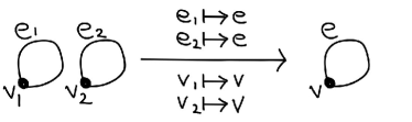
Figure 6: A flag surjective, but not flag bijective map. This is a valid of $\mathcal{G}$.

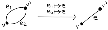
Figure 7: An example of a flag surjective but not flag bijective morphism of $\mathcal{G}$.

Figure 8: An example of an embedding (hence a flag bijective morphism) in $\mathcal{G}$.

Figure 10: This example is not a valid morphism in $\mathcal{G}$ because it does not respect Condition 2.

References

- [1]
- [2] Filippo Bonchi, Fabio Gadducci, Aleks Kissinger, Pawel Sobocinski & Fabio Zanasi (2016): Rewriting modulo symmetric monoidal structure. In: LiCS’16 Proceedings of the 31st Annual ACM/IEEE Symposium on Logic in Computer Science, pp. 707–719, 10.1145/2933575.2935316.
- [3] Filippo Bonchi, Fabio Gadducci, Aleks Kissinger, Pawel Sobocinski & Fabio Zanasi (2017): Confluence of Graph Rewriting with Interfaces. In: Proceedings of the 26th European Symposium on Programming Languages and Systems (ESOP’17), 10.1007/978-3-662-54434-1_6.
- [4] Bob Coecke, Ross Duncan, Aleks Kissinger & Quanlong Wang (2015): Generalised Compositional Theories and Diagrammatic Reasoning. In G. Chirabella & R. Spekkens, editors: Quantum Theory: Informational Foundations and Foils, Springer, 10.1007/978-94-017-7303-4_10.
- [5] Alexander Cowtan, Silas Dilkes, Ross Duncan, Alexandre Krajenbrink, Will Simmons & Seyon Sivarajah (2019): On the qubit routing problem. In Wim van Dam & Laura Mancinska, editors: 14th Conference on the Theory of Quantum Computation, Communication and Cryptography (TQC 2019), Leibniz International Proceedings in Informatics (LIPIcs) 135, pp. 5:1–5:32, 10.4230/LIPIcs.TQC.2019.5. Available at http://drops.dagstuhl.de/opus/volltexte/2019/10397.
- [6] Lucas Dixon & Ross Duncan (2009): Graphical Reasoning in Compact Closed Categories for Quantum Computation. Annals of Mathematics and Artificial Intelligence 56(1), pp. 23–42, 10.1007/s10472-009-9141-x.
- [7] Lucas Dixon, Ross Duncan & Aleks Kissinger (2010): Open Graphs and Computational Reasoning. In: Proceedings DCM 2010, Electronic Proceedings in Theoretical Computer Science 26, pp. 169–180, 10.4204/EPTCS.26.16.
- [8] Lucas Dixon & Aleks Kissinger (2013): Open Graphs and Monoidal Theories. Math. Structures in Comp. Sci. 23(2), pp. 308–359, 10.1017/S0960129512000138.
- [9] J. R. Edmonds (1960): A combinatorial representation for polyhedral surfaces. Notices of the American Mathematical Society 7(A646).
- [10] Hartmut Ehrig, Karsten Ehrig, Ulrike Prange & Gabriele Taentzer (2006): Fundamentals of Algebraic Graph Transformation. Monographs in Theoretical Computer Science, Springer Berlin Heidelberg, 10.1007/3-540-31188-2.
- [11] Jonathan L. Gross & Thomas W. Tucker (2001): Topological Graph Theory. Dover.
- [12] Lothar Heffter (1891): Über das Problem der Nachbargebiete. Mathematische Annalen 38(4), pp. 477–508, 10.1007/BF01203357.
- [13] A. Joyal & R. Street (1991): The Geometry of Tensor Categories I. Advances in Mathematics 88, pp. 55–113. 10.1016/0001-8708(91)90003-P.
- [14] G.M. Kelly & M.L. Laplaza (1980): Coherence for Compact Closed Categories. Journal of Pure and Applied Algebra 19, pp. 193–213, 10.1016/0022-4049(80)90101-2.
- [15] Aleks Kissinger & Vladimir Zamdzhiev (2015): Equational Reasoning with Context-Free Families of String Diagrams. In Francesco Parisi-Presicce & Bernhard Westfechtel, editors: Graph Transformation, Lecture Notes in Computer Science 9151, Springer International Publishing, pp. 138–154, 10.1007/978-3-319-21145-9_9.
- [16] S. Lack & P. Sobocinski (2003): Adhesive categories. Technical Report BRICS RS-03-31, BRICS, Department of Computer Science, University of Aarhus.
- [17] Stephen Lack & Pawel Sobocinski (2005): Adhesive and quasiadhesive categories. Theoretical Informatics and Applications 39(3), pp. 511 – 545, 10.1051/ita:2005028.
- [18] Peter Selinger (2011): A survey of graphical languages for monoidal categories. In Bob Coecke, editor: New structures for physics, Lecture Notes in Physics 813, Springer, pp. 289–355, 10.1007/978-3-642-12821-9_4.