Characterization of the HD 108236 system with CHEOPS and TESS. Confirmation of a fifth transiting planet

Abstract

Context. The HD 108236 system was first announced with the detection of four small planets based on TESS data. Shortly after, the transit of an additional planet with a period of 29.54 d was serendipitously detected by CHEOPS. In this way, HD 108236 ($V$=9.2) became one of the brightest stars known to host five small transiting planets (R_p¡3 R_⊕).

Aims. We characterize the planetary system by using all the data available from CHEOPS and TESS space missions. We use the flexible pointing capabilities of CHEOPS to follow up the transits of all the planets in the system, including the fifth transiting body.

Methods. After updating the host star parameters by using the results from Gaia eDR3, we analyzed 16 and 43 transits observed by CHEOPS and TESS, respectively, to derive the planets’ physical and orbital parameters. We carried out a timing analysis of the transits of each of the planets of HD 108236  to search for the presence of transit timing variations.

Results. We derived improved values for the radius and mass of the host star ($R_{\star}=0.876\pm 0.007$ $R_{\odot}$ and $M_{\star}=0.867_{-0.046}^{+0.047}$ $M_{\odot}$). We confirm the presence of the fifth transiting planet $f$ in a 29.54 d orbit. Thus, the HD 108236 system consists of five planets of R_b=1.587$\pm$0.028, R_c=2.122$\pm$0.025, R_d=2.629$\pm$0.031, R_e=3.008$\pm$0.032, and R_f=1.89$\pm$0.04 [R_⊕]. We refine the transit ephemeris for each planet and find no significant transit timing variations for planets $c$, $d,$ and $e$. For planets $b$ and $f$, instead, we measure significant deviations on their transit times (up to $22$ and $28$ min, respectively) with a non-negligible dispersion of 9.6 and 12.6 min in their time residuals.

Conclusions. We confirm the presence of planet $f$ and find no significant evidence for a potential transiting planet in a 10.9 d orbital period, as previously suggested. Further monitoring of the transits, particularly for planets $b$ and $f$, would confirm the presence of the observed transit time variations. HD 108236 thus becomes a key multi-planetary system for the study of formation and evolution processes. The reported precise results on the planetary radii – together with a profuse RV monitoring – will allow for an accurate characterization of the internal structure of these planets.

1 Introduction

Multi-planet systems are key to improving our understanding and studying the formation and evolution of planetary systems, with the ultimate goal of finding resemblances with the history of our own Solar System. The dynamics and architecture of multi-planet systems are crucial for imposing strong constraints on migration processes (e.g., Mills et al., 2016; Delisle, 2017; Leleu et al., 2021a). In addition, depending on the system, gravitational interaction between planets can produce detectable transit timing variations (TTVs), especially when planets are located close to mean motion resonances (Miralda-Escudé, 2002; Holman & Murray, 2005; Agol et al., 2005). In specific cases, TTVs can be used to estimate the masses of the planets without the requirement of complementary radial velocity observations (e.g., Barros et al., 2015; Gillon et al., 2017b; Freudenthal et al., 2018; Agol et al., 2021).

The amenability of the systems for in-depth characterizations, including comparative atmospheric studies through transmission spectroscopy, strongly depends on the brightness of the host star due to signal-to-noise considerations (see, e.g., the TSM metric in Kempton et al. (2018)). Thanks to the long baseline and high signal-to-noise ratios (S/N) of their observations, to date, most of the transiting multi-planet systems with four or more planets are part of the yield of the Kepler+K2 missions (Borucki et al., 2010; Howell et al., 2014), for which the magnitude distribution of the stellar hosts peaks towards $V\sim$15.

Table 1: Exoplanetary systems orbiting a bright stellar host (V$<10.5$), with more than three planets and at least one transiting planet.

System	V-mag	total number	number of	Pinner-Pouter	Reference
name		of planets	transiting planets	[d]
HD 219134	5.5	5(6)	2	3.1–46.8	Motalebi et al. (2015); Gillon et al. (2017a)
55 Cnc	5.95	5	1	0.73–4800	McArthur et al. (2004)
Kepler-444	8.9	5	5	3.6–9.7	Campante et al. (2015)
HIP 41378	8.9	5	5	15.6–324	Vanderburg et al. (2019)
HD 108236	9.2	5	5	3.79–29.5	Daylan et al. (2021); Bonfanti et al. (2021)
Kepler-37	9.8	4	4	13.3–39.8	Barclay et al. (2013)
V1298 Tau	10.1	4	4	8.24–60	David et al. (2019)
TOI-561	10.3	4(5)	4	0.45–77	Lacedelli et al. (2022)

In Table 1, we show the seven multi-planet systems known with more than three planets, among which there is at least one transiting a stellar host brighter than $V$=10.5. Kepler-444 is the brightest detected star ($V$=8.9) to host five transiting planets. It is an ultra-compact system formed by very small planets (radii ¡ 0.8 R_⊕) in orbital periods between 3.6 and 9.7 d. HIP 41378 ($V$=8.9, Vanderburg et al., 2019); it hosts two Sub-Neptune planets in orbits of 15.6 and 31.7 d and three additional large planets in long orbital periods ($\sim$130-324 d). Therefore, HD 108236 is the second-brightest stellar host of a multiple transiting-planet system in a compact architecture (periods ¡ 30 d). The HD 108236 system, also consisting of five transiting planets, is suitable for a complete and precise orbital and physical characterization thanks to the brightness of its host star.

The HD 108236 system was discovered by the TESS survey (TESS Object of Interest ID TOI 1233; Guerrero et al., 2021), and it was originally reported to consist of four transiting planets with orbital periods between 3.7-19.6 d and radii between 1.6-3.12 R_⊕ (Daylan et al., 2021). Its magnitude and location in the sky, makes it a perfect target for CHEOPS (Benz et al., 2021). As a follow-up mission, its goal is to provide ultra-high precision photometric observations of known exoplanet host stars for obtaining precise determinations of transiting exoplanet sizes. Bonfanti et al. (2021) used the first three CHEOPS light curves of HD 108236 system to refine the planetary transit ephemeris one year after the discovery observations. In addition, the analysis of these data revealed the presence of a fifth planet with 29.5 d orbital period. Here, we further characterize the HD 108236 system based on the analysis of the full CHEOPS observation dataset consisting of 15 light curves; together with all the available TESS data (i.e., with the addition of Sector 37). In this work, we confirm the presence of the fifth planet, $f,$ and we search for the 10.9 d transit signal of a putative sixth planet, which was suggested in the discovery paper.

In Sect. 2, we present the updated stellar host properties based on the updated input from Gaia eDR3. In Sect. 3, we describe the photometric observations used in this work, reporting 12 new CHEOPS light curves and all the available TESS data. The analysis of the data is described in Sect. 4. We describe the timing analysis of the transits in Sect. 5 and compare different approaches to estimate the planetary masses in Sect. 6. The discussion of the results and the conclusions of the work are presented in Sects. 7 and 8, respectively.

2 Host star properties

Bonfanti et al. (2021) already provided a thorough characterization of HD 108236. In this work, we assume the same spectroscopic parameters and elemental abundances, and we recall that they were derived from 13 high-resolution spectra (program 1102.C-0923, PI: Gandolfi) acquired by the High Accuracy Radial velocity Planet Searcher (HARPS, Mayor et al., 2003). In particular, $T_{\mathrm{eff}}$, $\log{g}$, and [Fe/H] were inferred from the ARES+MOOG tools (Sousa, 2014), while the elemental abundances were computed following the procedure detailed in Adibekyan et al. (2012, 2015). These values are reported in Table 2.

In taking advantage of the new stellar parallax from the third Gaia early data release (eDR3, Gaia Collaboration et al., 2021), we were able to update the stellar radius always through the infrared flux method (IRFM Blackwell & Shallis, 1977), which has already been summarized in Bonfanti et al. (2021). The slight refinement brought us to $R_{\star}$=$0.876\pm 0.007\,R_{\odot}$, which is fully compatible with what reported in Bonfanti et al. (2021). Using $T_{\mathrm{eff}}$, [Fe/H], and the new $R_{\star}$ estimate as input parameters, we then updated also the isochronal mass $M_{\star}$ and age $t_{\star}$ estimates. A first pair $(M_{\star,1},t_{\star,1})$ was computed employing the isochrone placement technique (Bonfanti et al., 2015, 2016) within PARSEC v1.2S evolutionary models (Marigo et al., 2017), while a second pair $(M_{\star,2},t_{\star,2})$ was outputted by the CLES code (Code Liègeois d´Évolution Stellaire, Scuflaire et al., 2008), following the fitting procedure described in Salmon et al. (2021). We finally combined the two respective estimates after carefully checking their mutual consistency through the $\chi^{2}$-based criterion outlined in Bonfanti et al. (2021), ending up with the following results: $M_{\star}$=$0.867_{-0.046}^{+0.047}\,M_{\odot}$ and $t_{\star}$=$6.7_{-3.4}^{+3.3}$ Gyr. All the relevant stellar parameters are listed in Table 2 and we note that all the updated parameters are consistent with what computed by Bonfanti et al. (2021) well within 1$\sigma$.

Table 2: Stellar properties of HD 108236.

HD 108236
Alternative names	TOI-1233
	HIP 60689
	TIC 260647166
	Gaia DR2 6125644402384918784
Parameter	Value	Source
R.A. [J2000]	12:26:17.89	Gaia DR2
DEC. [J2000]	-51:21:46.21	Gaia DR2
$V$ [mag]	9.24	Simbad
$G$ [mag]	9.0875	Simbad
$J$ [mag]	8.046	Simbad
$T_{\mathrm{eff}}$ [K]	$5660\pm 61$	Spectroscopy
$\log{g}$ [cgs]	$4.49\pm 0.11$	Spectroscopy
[Fe/H] [dex]	$-0.28\pm 0.04$	Spectroscopy
[Mg/H] [dex]	$-0.27\pm 0.03$	Spectroscopy
[Si/H] [dex]	$-0.29\pm 0.02$	Spectroscopy
Updated values
$d$ [pc]	$64.66\pm 0.05$	Gaia parallax
$\theta$ [mas]	$0.1261\pm 0.0010$	IRFM
$R_{\star}$ [$R_{\odot}$]	$0.876\pm 0.007$	IRFM
$M_{\star}$ [$M_{\odot}$]	$0.867_{-0.046}^{+0.047}$	Isochrones
$t_{\star}$ [Gyr]	$6.7_{-3.4}^{+3.3}$	Isochrones
$L_{\star}$ [$L_{\odot}$]	$0.707\pm 0.032$	from $R_{\star}$ and $T_{\mathrm{eff}}$
$\rho_{\star}$ [g/cm3]	$1.79\pm 0.11$	from $R_{\star}$ and $M_{\star}$

3 Observations

Here, we describe the photometric data used for the modeling of the system from both CHEOPS and TESS space missions.

3.1 CHEOPS

We obtained 15 CHEOPS observation runs (visits) of HD 108236, accumulating $\sim$8.5 d on target, of which $\sim$3.9 d were not covered due to Earth occultations or South Atlantic Anomaly (SAA) crossings by the satellite. With CHEOPS, we observed a total of 16 planetary transits of the system, as reported in the observation log in Table 3. The raw data of each visit were automatically processed by CHEOPS Data Reduction Pipeline (DRP, v13 Hoyer et al., 2020). In short, the DRP performs the instrumental calibration (bias, gain, linearization, and flat-fielding correction) and the environmental correction (cosmic ray hits, background, and smearing correction) before extracting the photometric signal of the target in four different aperture sizes. Three of these apertures have a fixed radius (RINF=22.5 pix, DEFAULT=25 pix, RSUP=30 pix) while a fourth, ROPT, is chosen automatically based on the contamination present in the Field of View (FoV). The contamination is computed by DRP using simulations of the FoV based on the Gaia catalog (Gaia Collaboration et al., 2018). This information, together with other correction times series (e.g., background, smearing), are provided in the final DRP products along with the photometric time series, to be used in the analysis and detrending of the light curves. In this work, we use the light curves obtained with the DEFAULT aperture, as it produces the raw curves with the lowest dispersion when compared to the other photometric apertures.

Table 3: Log of the CHEOPS observations of HD 108236. The second column shows the planetary transits observed during each CHEOPS visit. The last column shows the observation efficiency of each visit, considering the gaps produced by Earth occultations or SAA crossings. We report the unique identifiers of each CHEOPS visit: OBSID and File Key.

id	Planets	File Key	OBSID	Start date	Duration	Exp. time	Efficiency
#				[UTC]	[h]	[s]	[%]
1	c, e, (g)	CH_PR300046_TG000101_V0200	1015572	2020-03-10T18:09:15.91	18.33	42.0	61.1
2	b	CH_PR100031_TG015701_V0200	1084970	2020-04-19T08:48:11.23	17.04	49.0	59.6
3	d	CH_PR100031_TG015401_V0200	1088211	2020-04-28T07:06:11.05	18.63	49.0	54.8
4	c	CH_PR100031_TG015601_V0200	1088443	2020-04-29T16:02:11.28	11.24	49.0	53.7
5	b, f	CH_PR100031_TG015702_V0200	1087957	2020-04-30T17:06:11.04	16.40	49.0	54.5
6	c	CH_PR100031_TG015602_V0200	1096738	2020-05-05T21:36:10.33	10.57	49.0	57.1
7	c	CH_PR100031_TG022401_V0200	1107339	2020-05-12T02:10:11.27	07.08	49.0	57.5
8	b	CH_PR100031_TG023001_V0200	1111865	2020-05-19T23:34:51.37	08.91	49.0	56.6
9	d, (g)	CH_PR100031_TG024301_V0200	1117140	2020-05-26T09:18:11.28	26.37	49.0	51.0
10	b	CH_PR100031_TG023002_V0200	1117572	2020-05-27T14:31:10.32	08.35	49.0	47.6
11	e	CH_PR100031_TG022701_V0200	1117376	2020-05-28T05:21:10.39	13.14	49.0	50.4
12	b	CH_PR100031_TG023003_V0200	1124008	2020-05-31T09:24:11.59	08.89	49.0	52.8
13	c	CH_PR100031_TG022901_V0200	1124302	2020-06-05T22:42:30.53	10.38	49.0	51.6
14	f	CH_PR110045_TG002601_V0200	1458282	2021-04-20T06:58:13.84	10.95	49.0	62.2
15	(g)	CH_PR110045_TG002701_V0200	1456848	2021-04-29T18:51:51.55	17.98	49.0	53.9

3.2 TESS

Similarly to Daylan et al. (2021) and Bonfanti et al. (2021), our analysis includes the TESS data of HD 108236, consisting of the 2 min light curves obtained during the monitoring of Sectors 10 and 11. Additionally, we incorporated the 2 min Sector 37 data, collected by TESS camera 2, between 2021-04-02 and 2021-04-28, during its second pass of the Southern Hemisphere. Here, we also use the Presearch Data Conditioning Simple Aperture Photometry (PDC-SAP, Stumpe et al., 2012, 2014; Smith et al., 2012) as provided by the Science Processing Operations Center (SPOC, Jenkins et al., 2016). In the TESS data, we identified and analyzed 18 transits of planet b, 12 transits of planet c, 6 transits of planet d, 4 transits of planet e, and 3 transits of planet f. In order to reduce processing times in the analysis, in this work we used only the portions of the TESS light curves with detected transits (leaving enough out-of-transit data for further detrending), ending up with 34 single light curves which we treated individually; among them, 4 light curves present consecutive transits of two planets and other 5 light curves show overlapped transits (transit events of two planets occurring simultaneously).

4 System modeling

4.1 Detrending of CHEOPS light curves

CHEOPS rotates around the line of sight while observing. Together with the extended shape of the CHEOPS PSF, this can produce different effects that perturb the aperture photometry (see e.g., Hoyer et al., 2020; Lendl et al., 2020; Bonfanti et al., 2021; Maxted et al., 2022). Some of these effects are the varying contaminating flux from nearby rotating background stars, moving smear trails of bright stars, and the reflections imprinted in the detector produced by different astrophysical sources close to CHEOPS pointing direction. All of these effects vary with the roll angle of the satellite and as a result, the flux of the raw target’s light curve is correlated with the roll angle. Therefore, in most cases, a proper detrending against this parameter is fundamental to exploit the exquisite CHEOPS photometry. Following Bonfanti et al. (2021), we modeled the flux versus the roll angle pattern of each CHEOPS light curve through Gaussian processes (GPs, Rasmussen & Williams, 2005). In particular, we adopted a Matérn-3/2 kernel and used the GP predictor implemented in the celerite package (Foreman-Mackey et al., 2017), which provides the GP model and its variance. Finally, we obtained the roll-angle detrended light curves, while also adjusting the flux error bars to account for the further variance introduced by the GP modeling. In order to reduce the number of fitted parameters, we used these roll angle detrended CHEOPS light curves in the following transits modeling. The CHEOPS raw and detrended light curves are reported in Appendix A (Fig. 11, 12, and 13).

4.2 Transit modeling

For the analysis of CHEOPS and TESS light curves, we used the juliet package (Espinoza et al., 2019), which implements the modeling of transit light curves from batman (Kreidberg, 2015) in a Bayesian framework using the dynesty nested sampling tool (Speagle, 2020). We performed the modeling of the full system (star+five planets) using all the CHEOPS (15 roll-angle detrended light curves, as described in Sect. 4.1) and TESS (34) light curves. In this configuration, we are able to retrieve, for example, an estimation of the orbital period (P) and reference time (T₀) for each planet. We used as reference the values published in Bonfanti et al. (2021) to define our priors. In general, we used normal distributions centered in their results, but wide enough to ensure they are weakly informative. For the priors of the transit reference time (T₀) of each planet, when possible, we used TESS epochs which do not correspond to overlapped transits to mitigate potential time offsets. We also adopted the same constraints in the eccentricity ($e<0.1$) resulting from dynamical stability simulations of the system; and the values for the quadratic limb darkening coefficients ($q_{1}$, $q_{2}$) for CHEOPS and TESS passbands (see Bonfanti et al. (2021) for details). In addition, juliet allows us to directly fit the stellar density ($\rho_{\star}$), instead of fitting the scaled semi-major axis for each planet. Therefore, we used the value of stellar density derived from the updated stellar parameters (described in Sect. 2) as a truncated-normal prior in the modeling. We also fit for a photometric offset ($mflux$) and a ”jitter” noise term ($\sigma_{w}$) for each light curve. As the contamination by external sources is small and already corrected in CHEOPS light curves by the roll angle detrending (described in Sect. 4.1), we fixed the dilution factor of each light curve, $mdilution$=1. In addition, we fit for a linear and quadratic temporal term ($c_{1}(t)$ and $c_{2}(t^{2})$) to take care of any residual trend remaining in the CHEOPS transits. Any additional free parameters of our joint fit were the orbital period (P), reference time (T₀), planet-to-star radius ratio (R_p/R_⋆), and the impact parameter ($b$) of each planet. The eccentricity ($e$) and the argument of periastron passage ($\omega$) of the orbit were estimated using the parametrization ($\sqrt{e}sin(\omega)$,$\sqrt{e}cos(\omega)$). For these two parameters and the impact parameter, $b$, we used Uniform prior distributions. The value of the scaled semi-major axis of the orbit ($a$/R_⋆) for each planet was derived directly from the fitted $\rho_{\star}$, P, and Kepler’s third law. All the priors used in the modeling are listed in Table 8. The fitted and derived planetary parameters from the posterior distributions of the system are shown in Table 4, while the phased light curves together with the best fit model are presented in Fig. 1 and 2 for CHEOPS and TESS data, respectively. The individual detrended light curves with the best fit model overplotted are shown in Figs. 12 and 13.

To confirm our results, we also performed an independent analysis of all the data with the Allesfitter package (Günther & Daylan, 2021, 2019), following a similar procedure as described in Bonfanti et al. (2021). We imposed Normal priors on the mean stellar density $\rho_{\star}$ and on the LD coefficients. For all the other system parameters, we adopted wide uniform priors. An upper limit of 0.1 on the orbital eccentricity was also imposed. The temporal detrending benefited of the GP treatment (Matérn-3/2 kernel) for the three TESS sectors, while we used splines for the 15 CHEOPS observations (already pre-detrended against roll-angle following Sect. 4.1) to avoid a dramatic increase of the number of fitted parameters. The resulting parameters are fully consistent, well within $\pm 1\sigma$ level in most of the cases, with the results obtained from the juliet analysis. We notice that orbital eccentricities listed in Table 4 are high when compared to what is expected for multiplanetary systems. We performed a series of tests to explore the possible cause, and finally we attribute the results to the parameterizations used by juliet. In any case, a more detailed RV analysis will provide a final estimate of the eccentricities, something that the photometry presented in this work cannot solve on its own. We describe the performed tests in Appendix C. We also confirm that the rest of the other modeled parameters are robust, no matter the approach used to fit $e$ and $\omega$.

Table 4: Fitted and derived parameters of the HD 108236 system from CHEOPS and TESS transits.

	HD 108236
Quadratic L. D. Coeff.	$q_{1}$	$q_{2}$		$q_{1}$	$q_{2}$
CHEOPS	$0.446^{+0.016}_{-0.018}$	$0.341^{+0.017}_{-0.014}$	TESS	$0.277^{+0.018}_{-0.023}$	$0.230^{+0.016}_{-0.021}$
Fitted parameter	Planet $b$	Planet $c$	Planet $d$	Planet $e$	Planet $f$
Orbital Period, P [d]	$3.7958785^{+0.0000076}_{-0.0000070}$	$6.2036717^{+0.0000092}_{-0.000010}$	$14.175818^{+0.000024}_{-0.000023}$	$19.5901277^{+0.000030}_{-0.000030}$	$29.53935^{+0.00012}_{-0.00014}$
T0 [BJD-2 450 000.]	$8572.11017^{+0.00062}_{-0.00068}$	$8572.39445^{-0.00067}_{-0.00065}$	$8571.33678^{+0.00061}_{-0.00059}$	$8586.56741^{+0.00056}_{-0.00055}$	$8616.0403^{+0.0014}_{-0.0014}$
Rp/R⋆	$0.01661^{+0.00025}_{-0.00026}$	$0.02221^{+0.00020}_{-0.00018}$	$0.02751^{+0.00025}_{-0.00024}$	$0.03148^{+0.00023}_{-0.00023}$	$0.01979\pm 0.00043$
$\sqrt{e}sin(\omega)$	$0.221^{+0.043}_{-0.055}$	$0.154^{+0.043}_{-0.068}$	$-0.159^{+0.051}_{-0.067}$	$0.257^{+0.025}_{+0.035}$	$-0.028^{+0.072}_{-0.076}$
$\sqrt{e}cos(\omega)$	$0.120^{+0.066}_{-0.065}$	$-0.256^{+0.047}_{-0.028}$	$-0.217^{+0.084}_{-0.051}$	$-0.048^{+0.062}_{-0.070}$	$0.129^{+0.072}_{-0.076}$
Impact parameter, $b$ [R⋆]	$0.322^{+0.060}_{-0.057}$	$0.308^{+0.055}_{-0.046}$	$0.519^{+0.029}_{-0.026}$	$0.392^{+0.032}_{-0.029}$	$0.701^{+0.020}_{-0.021}$
Derived parameter
Rel. semi-major axis, a/R⋆	$11.080^{+0.046}_{-0.043}$	$15.373^{+0.064}_{-0.059}$	$26.67^{+0.11}_{-0.10}$	$33.10^{+0.14}_{-0.13}$	$43.51^{+0.18}_{-0.17}$
Eccentricity, $e$	$0.067^{+0.025}_{-0.026}$	$0.091^{+0.021}_{-0.033}$	$0.075^{+0.021}_{-0.022}$	$0.073^{+0.014}_{-0.017}$	$0.024^{+0.024}_{-0.016}$
Arg. of periastron, $\omega$ [∘]	$61^{+15}_{-14}$	$149^{+11}_{-7}$	$144^{+12}_{-22}$	$101^{+15}_{-14}$	$24^{+34}_{-17}$
Orbital inclination, $i$ [∘]	$88.23\pm 0.32$	$88.8\pm 0.2$	$88.8\pm 0.1$	$89.3\pm 0.1$	$89.07\pm 0.03$
Planet radius [R⊕]	$1.587\pm 0.028$	$2.122\pm 0.025$	$2.629\pm 0.031$	$3.008\pm 0.032$	$1.89\pm 0.04$
Semi-major axis, a [AU]	$0.0451\pm 0.0004$	$0.0626\pm 0.0006$	$0.1087\pm 0.0010$	$0.1348\pm 0.0012$	$0.1773\pm 0.0016$
Equilibrium temp. T${}_{\text{eq}}$ [K]	$1202\pm 13$	$1021\pm 11$	$775\pm 8$	$696\pm 8$	$607\pm 7$
Transit duration, T${}_{\text{I-IV}}$ [h]	$2.45\pm 0.06$	$2.93\pm 0.06$	$3.52\pm 0.08$	$4.16\pm 0.07$	$3.8\pm 0.1$

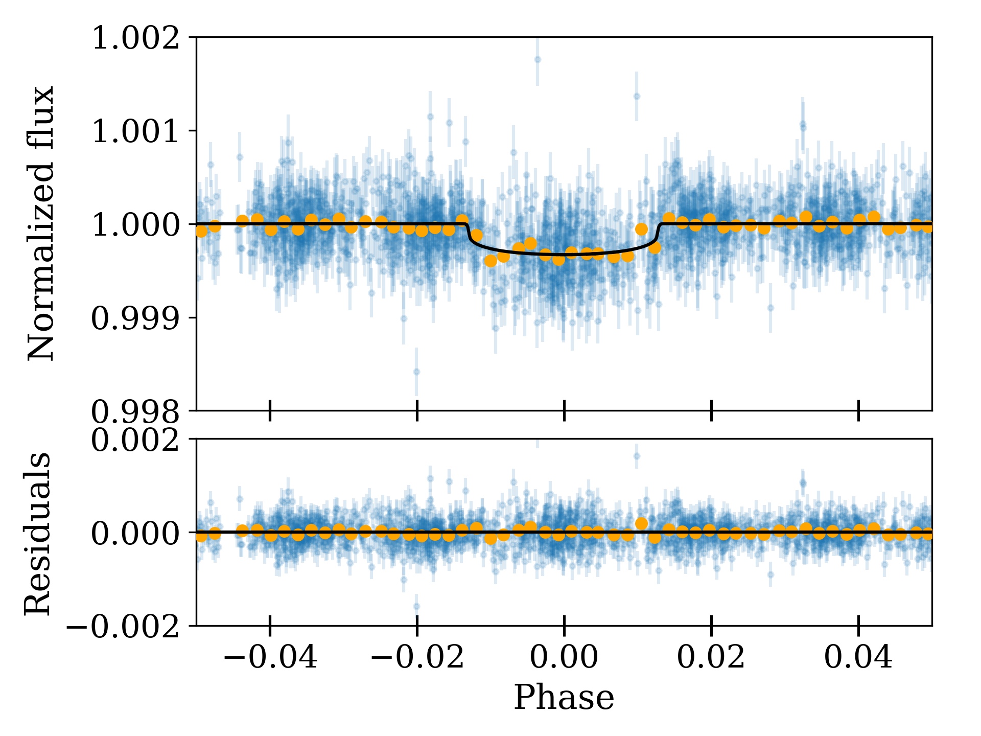
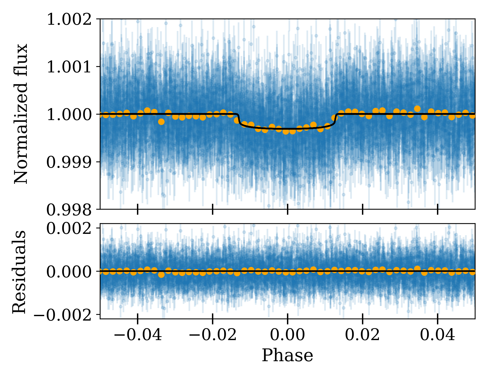
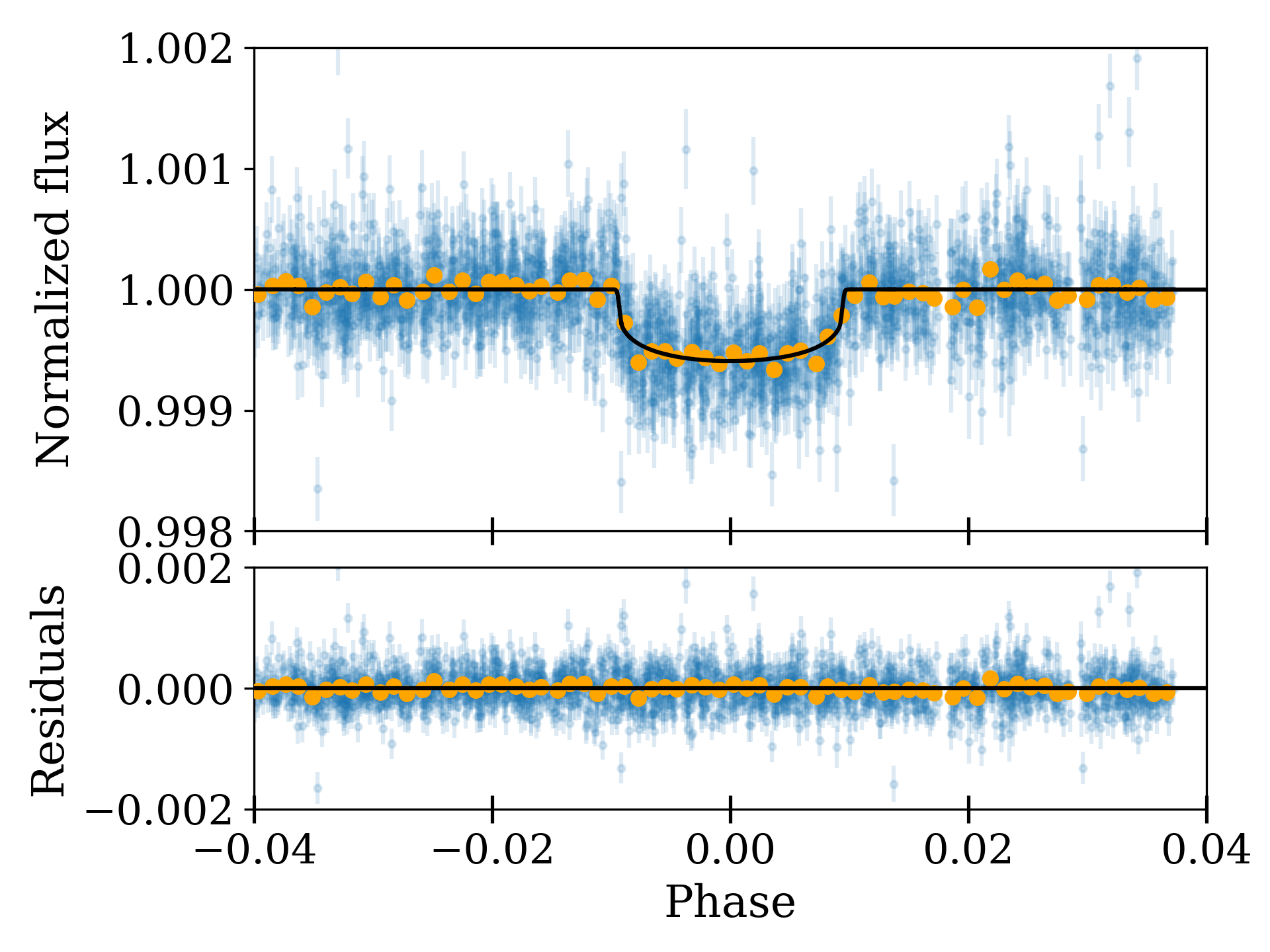
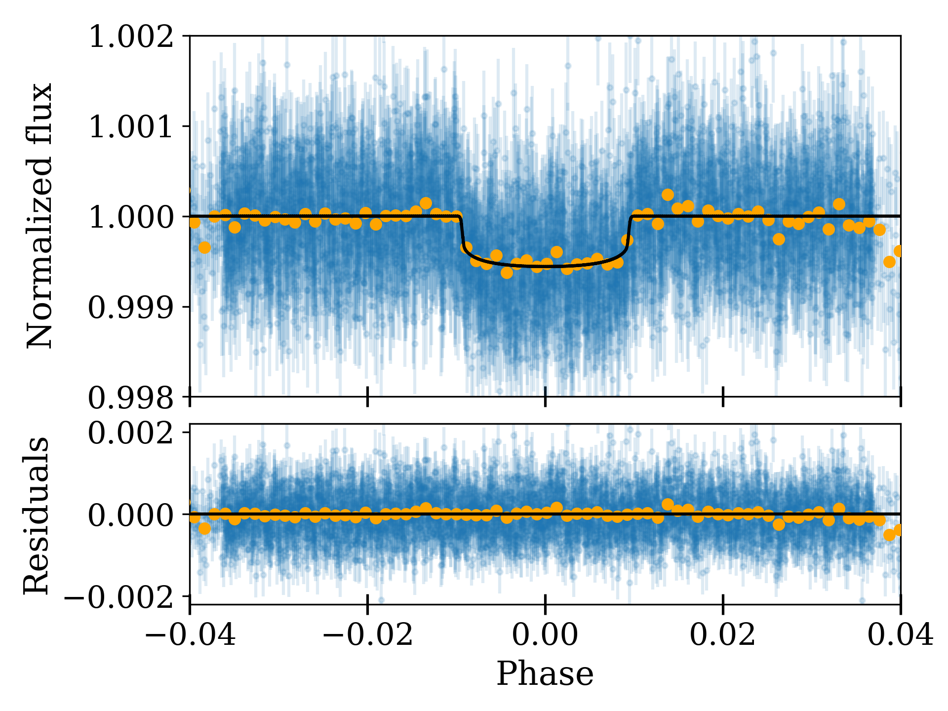
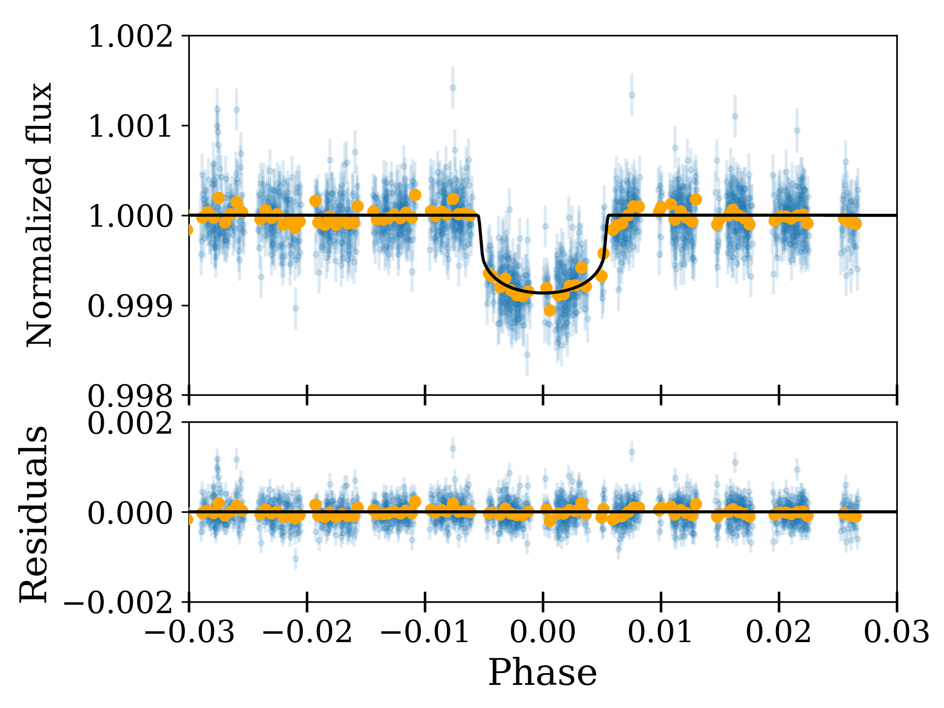
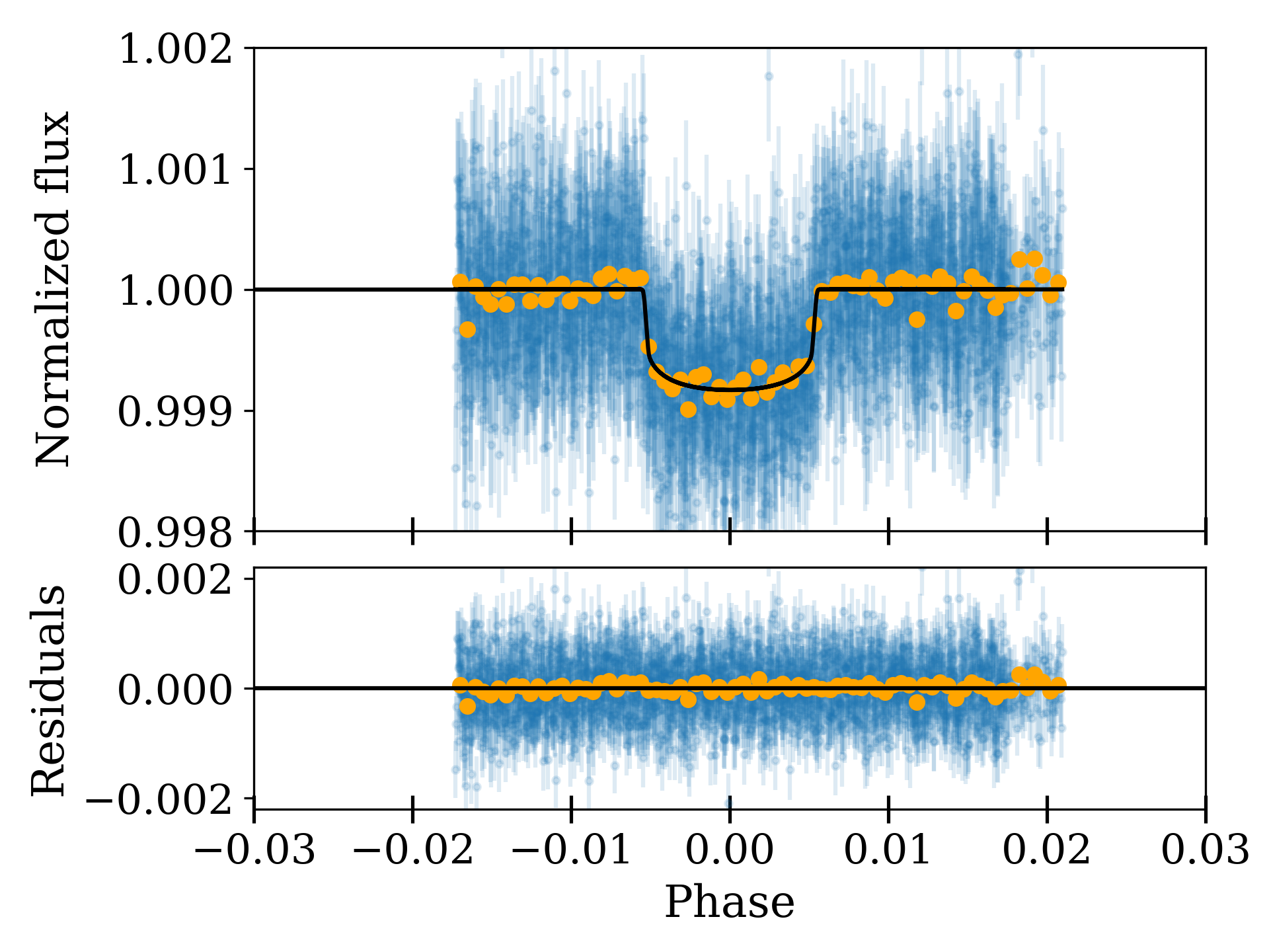
Figure 1: Phased CHEOPS (left) and TESS (right) light curves (blue dots) and its 10-min bins (yellow points). The best transit models (solid black curves) for planets $b$, $c$ and $d$ (from top to bottom) obtained in the global analysis of the data are shown; together with the respective residuals (thin bottom panels). Additional transit events of other planets were removed before plotting the final phased curve.

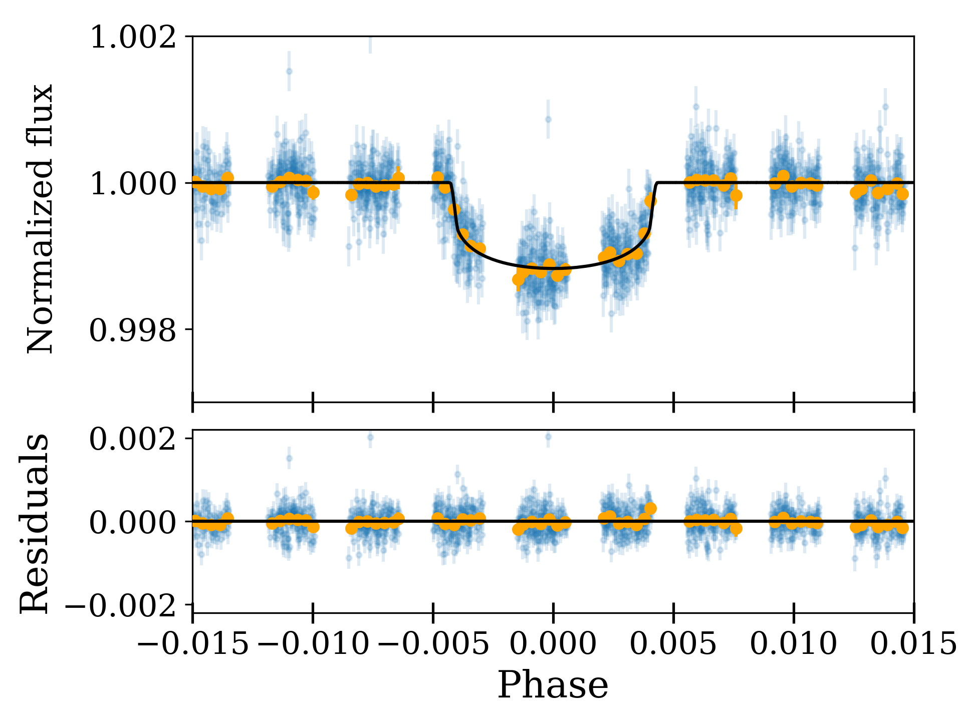
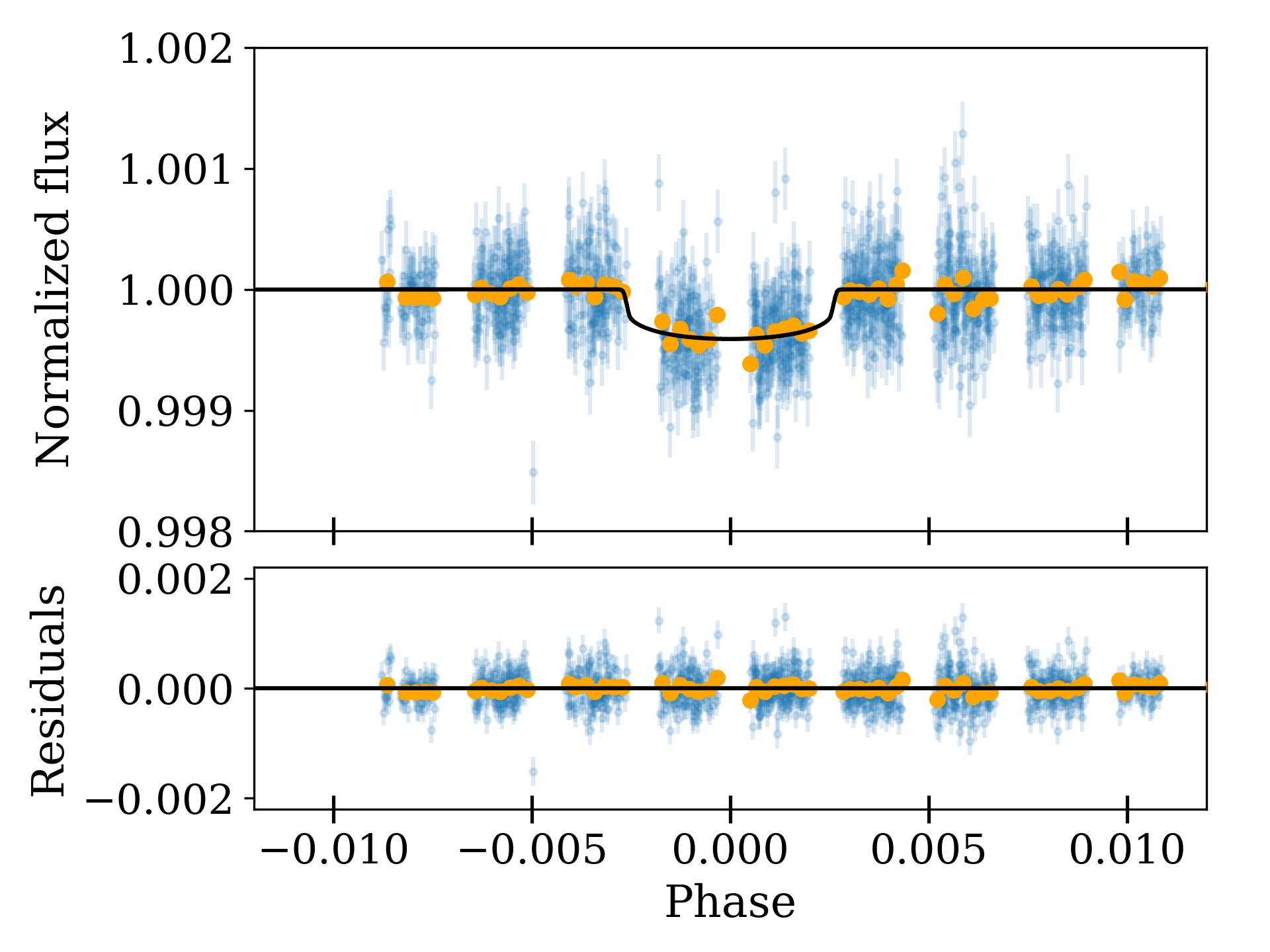
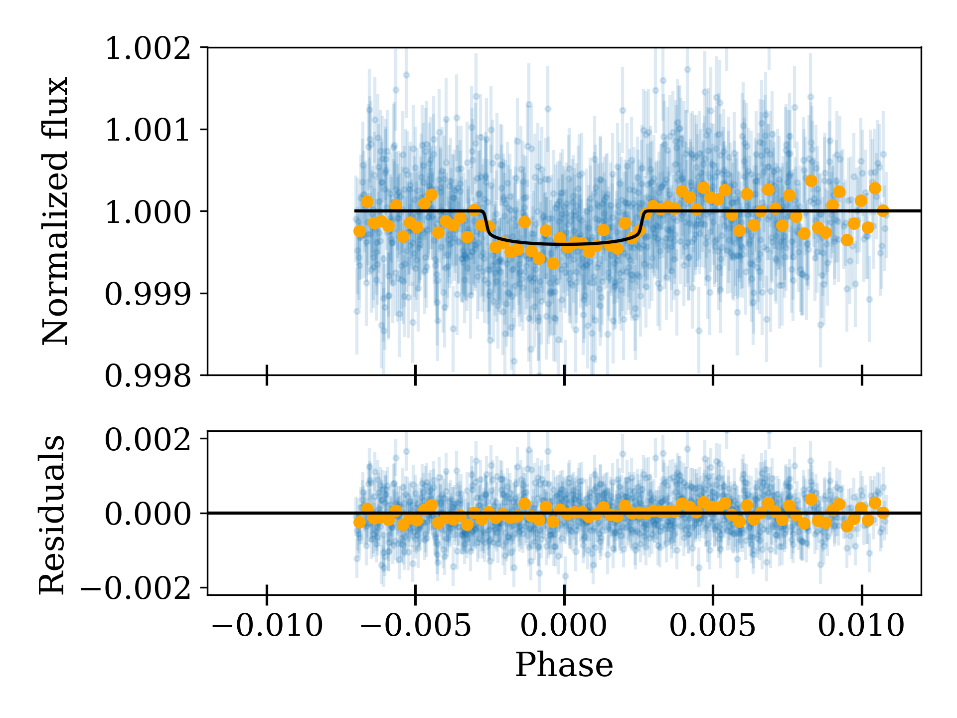
Figure 2: Phased CHEOPS (left) and TESS (right) light curves (blue dots) and its 10-min bins (yellow points). The best transit models (solid black curves) for planet $e$ (top) and $f$ (bottom) obtained in the global analysis of the data. Same details as in Fig. 1.

4.3 Confirmation of planet $f$

As described in Bonfanti et al. (2021), an additional transit-like feature was serendipitously detected in the CHEOPS light curve when monitoring a transit of planet $b$ (see top panel in Fig. 3). They also found signals in Sectors 10 and 11 of the TESS data that are consistent with a planetary candidate $f$ with an orbital period of 29.54 d. We detected transits of planet $f$ in the TESS Sectors 10 and 11, as well as in Sector 37, which are consistent with the 29.54 d period. The fact that two consecutive transits were identified in the first TESS Sector (as reported in Table 10) and no other transit consistent with this planet was detected in the TESS light curves in that time excludes the viability of the 29.54 d period aliases. The TESS phased light curve is presented at the bottom-right panel of Fig. 2. To confirm the presence of this planet, we scheduled a dedicated CHEOPS visit (observation 14 in Table 3) to observe a single transit of this planet. We present in Fig. 3 the light curve obtained from this observation together with the best-fit model resulting from the analysis of CHEOPS and TESS data. In Fig. 3, we also show the light curve reported in Bonfanti et al. (2021) with a transit of both $b$ and $f$ planets. The phased version of the combined two CHEOPS light curves is shown in the bottom-left panel of Fig. 2.

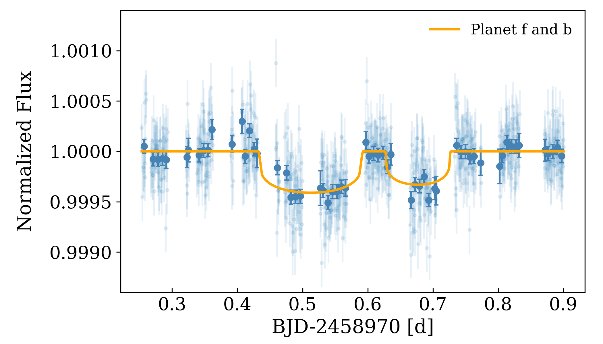
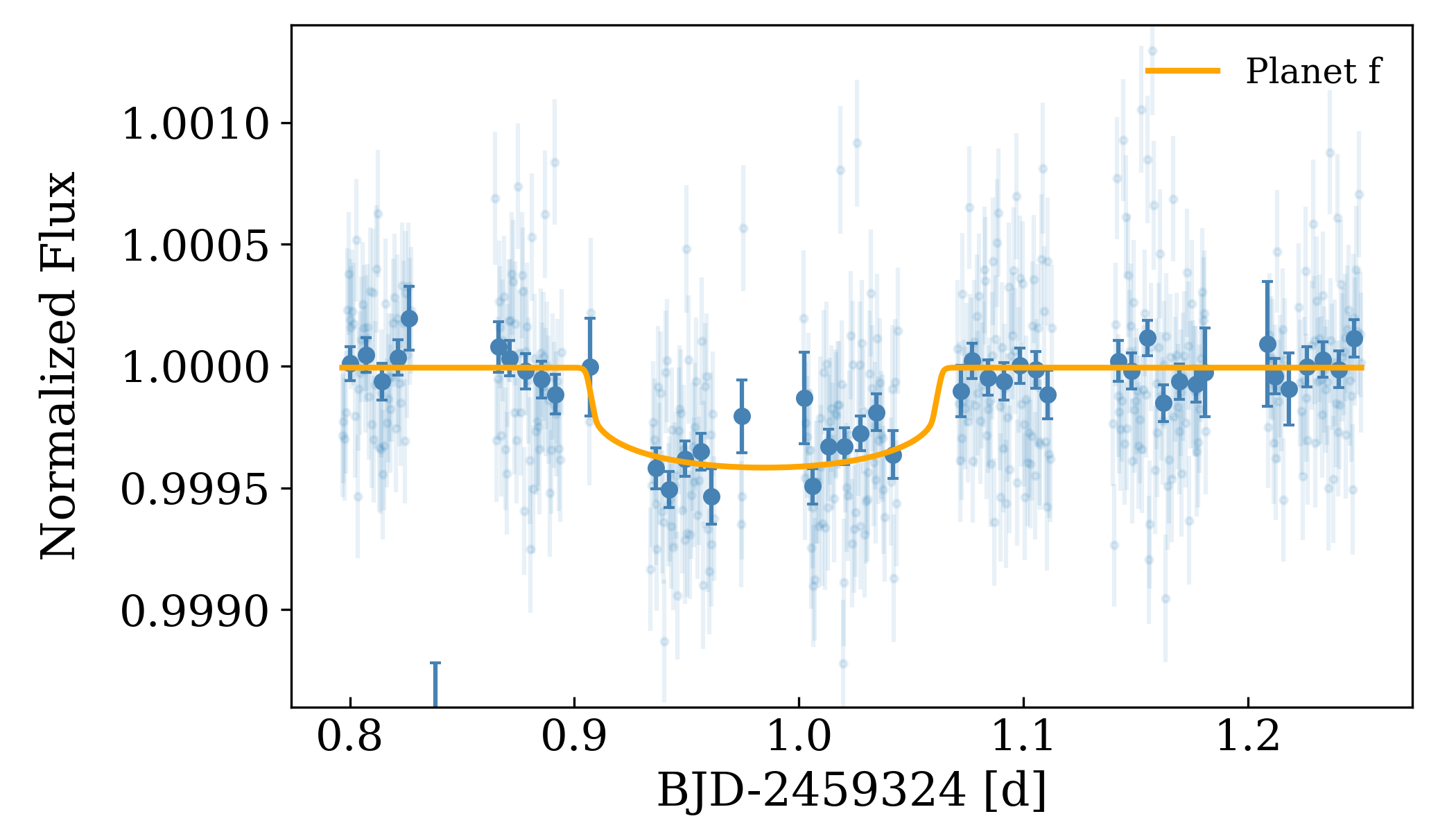
Figure 3: CHEOPS light curve of HD 108236 during a transit of planet $f$ ($\sim$2 458 970.5 BJD) and $b$ ($\sim$2 458 970.7 BJD) (top panel), as well as during a dedicated observation of a planet $f$ transit (bottom panel). Detrended photometric points and its 10 min bins are represented by light and dark blue dots, respectively. The best model for each planet is represented by the yellow curve.

4.4 Non-detection of a putative planet $g$

Daylan et al. (2021) reported a hint of a $\sim$10.9 d periodic transit signal in TESS data with amplitude of 230 ppm (without excluding a possible instrumental origin). Based on the ephemeris reported in that work (T₀ = 2 458 570.6781 BJD and P = 10.9113 d), we can see that this planet should have transited during the CHEOPS observations 1 and 9 (see the light curves in upper and middle panels of Fig. 4, respectively), but no clear evidence of this has been detected. Observation 1 has already been published by Bonfanti et al. (2021), who noticed that the transit of this putative planet would have occurred at T${}_{0}=2\,458\,919.84$ BJD, being partially overlapped with the transit of planet $c$. They performed a comparative analysis of a five-planet versus six-planet scenario, finding that there was no strong evidence to reject the five-planet scenario based on the Bayes factors of the two models. According to its ephemeris, the hypothetical planet $g$ would transit at T${}_{0}=2\,458\,996.22$ BJD during observation 9 (Fig. 4, middle panel). In the time of that CHEOPS visit, we actually noticed a short flux decrease, but it was shifted 0.13 d from the linear ephemeris at $\sim$2 458 996.35 BJD. The amplitude of this flux decrease is $\sim$125 ppm, which is around half of what was reported by Daylan et al. (2021) in TESS data. To further probe this periodic signal, we scheduled a $\sim$18 h CHEOPS observation, taking special care to avoid any overlap with the transits of the other five planets in the system (observation 15 in Table 3). In Fig. 4 (bottom panel), we show the detrended light curve of this observation where we found no significant evidence of any transit-like signal. We observed a shallow flux decrease centered at $\sim$2 459 334.53 BJD (linear ephemeris would predict T${}_{0}=2\,459\,334.47$ BJD), but also consistent with other features present in the light curve, which likely are residuals of the detrending of the well-known systematics of CHEOPS photometry as a function of its rotation angle. Despite this, we performed additional statistical tests to confirm that the detection of this transit-like feature is not significant (see Appendix D for details). We conclude that with the data we have on hand, we cannot confirm the presence of this additional planet $g$ in the system. In fact, a planet with a 10.9 d period would have a transit duration between 3.7-4 h (assuming a circular orbit and a zero impact parameter). The rms of the light curve of the CHEOPS observation 15 (bottom panel in Fig. 4) at these timescales corresponds to 17–20 ppm, which translates into an upper limit in the size of an undetected planet of 0.42 R_⊕ (with $e=b=0$) at S/N=1.

Taking into account that a transit of this putative planet was not observed in any of the CHEOPS light curves, we can assess the period range around P=10.9113 d. Using only CHEOPS data we can rule out a period in this range assuming that the errors in the ephemeris are given by the orbital period only, that is, fixing T₀ to the value reported by Daylan et al. (2021). Thus, we can discard periods in the range P=$10.9113^{+0.052}_{-0.018}$ d using CHEOPS data only. We note that the accumulation of these uncertainties in the orbital period will translate into offsets of more than 20 h at CHEOPS epochs. Moreover, no transits were detected at the expected times in the TESS Sector 37. Additionally, we used the transit least-squares tool (TLS Hippke & Heller, 2019) to search for other transits in this TESS light curve. After masking the transits of the known planets, no significant signals were found with periods between 0.52$-$24.5 d.

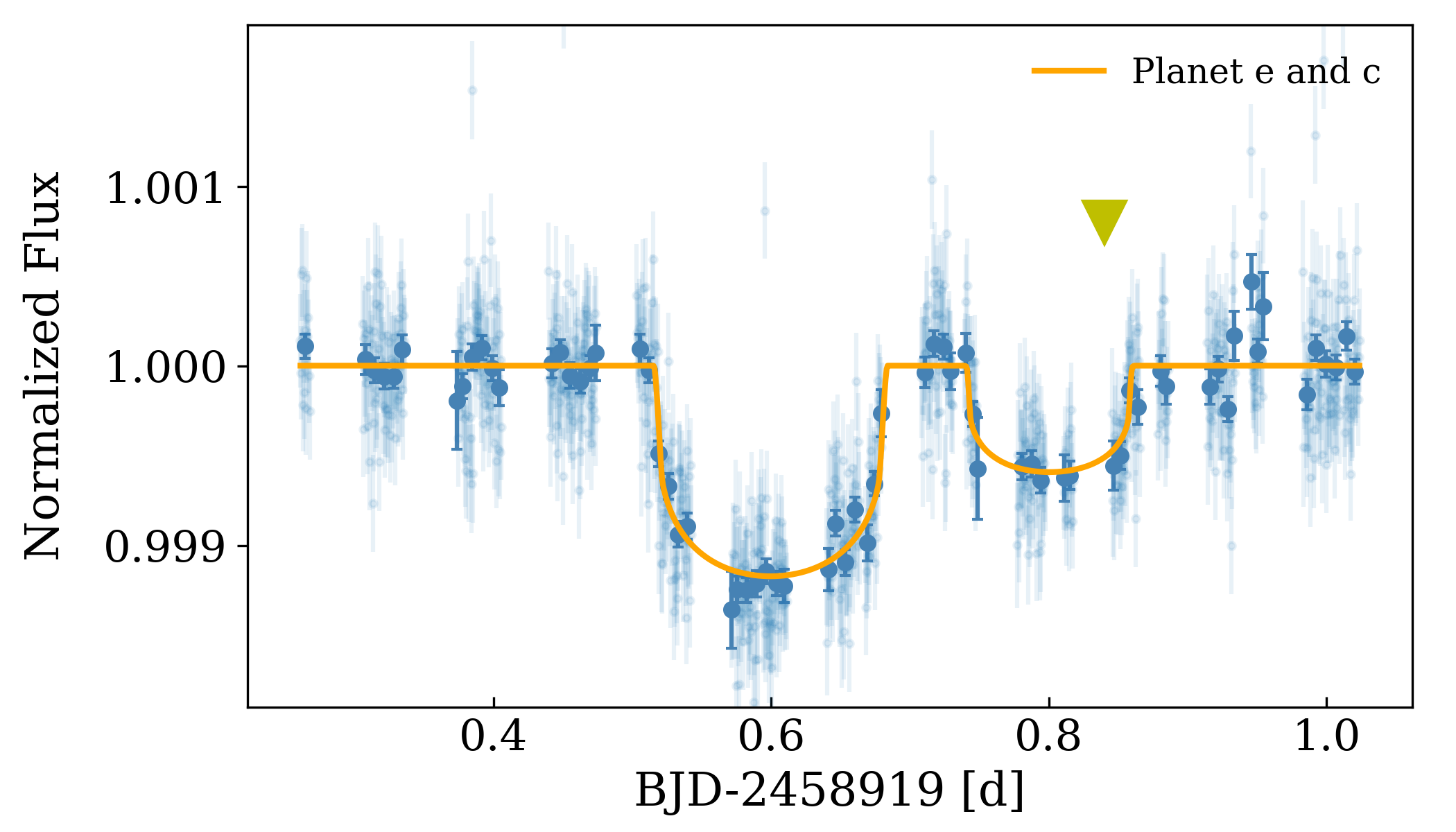
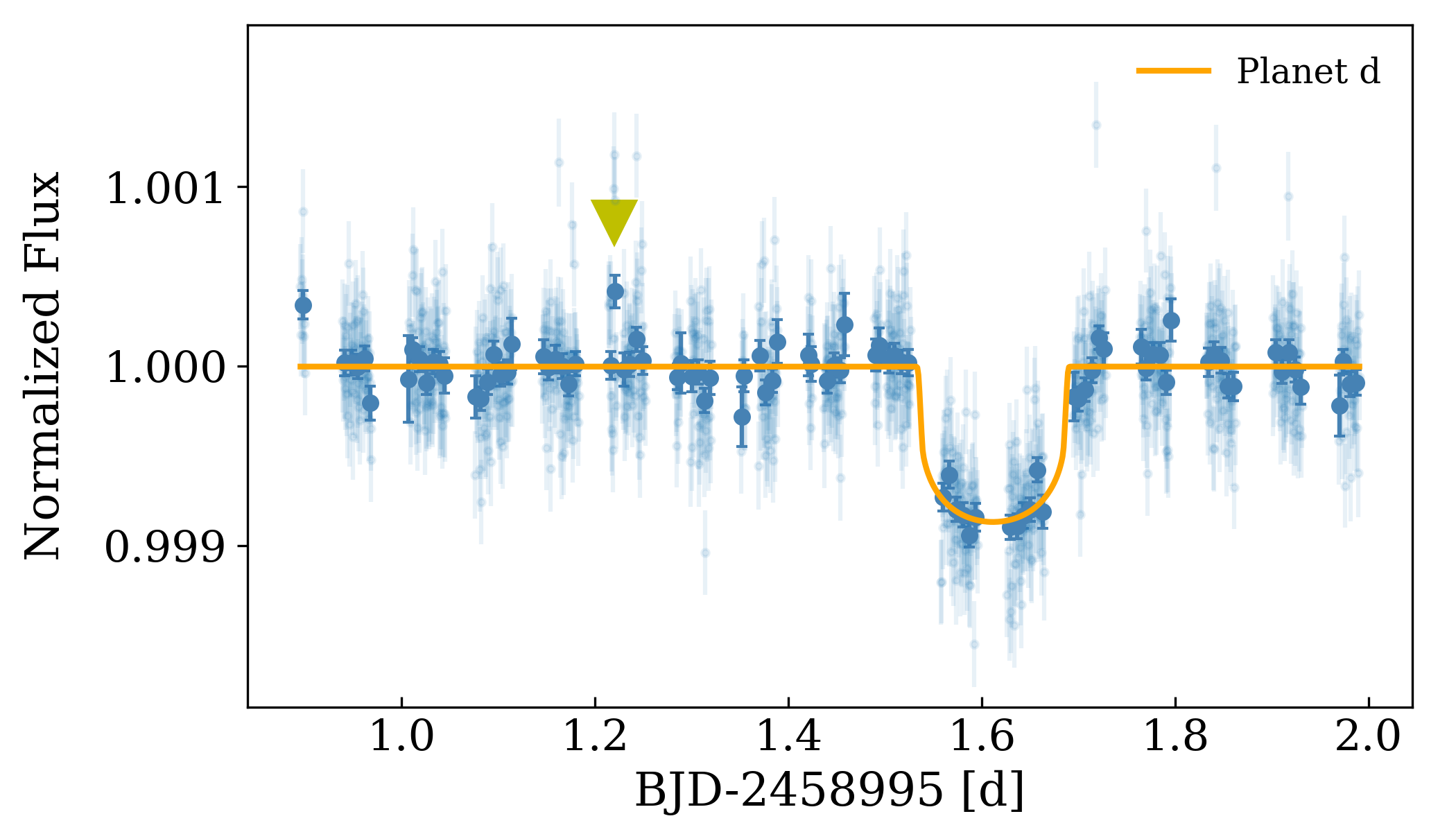
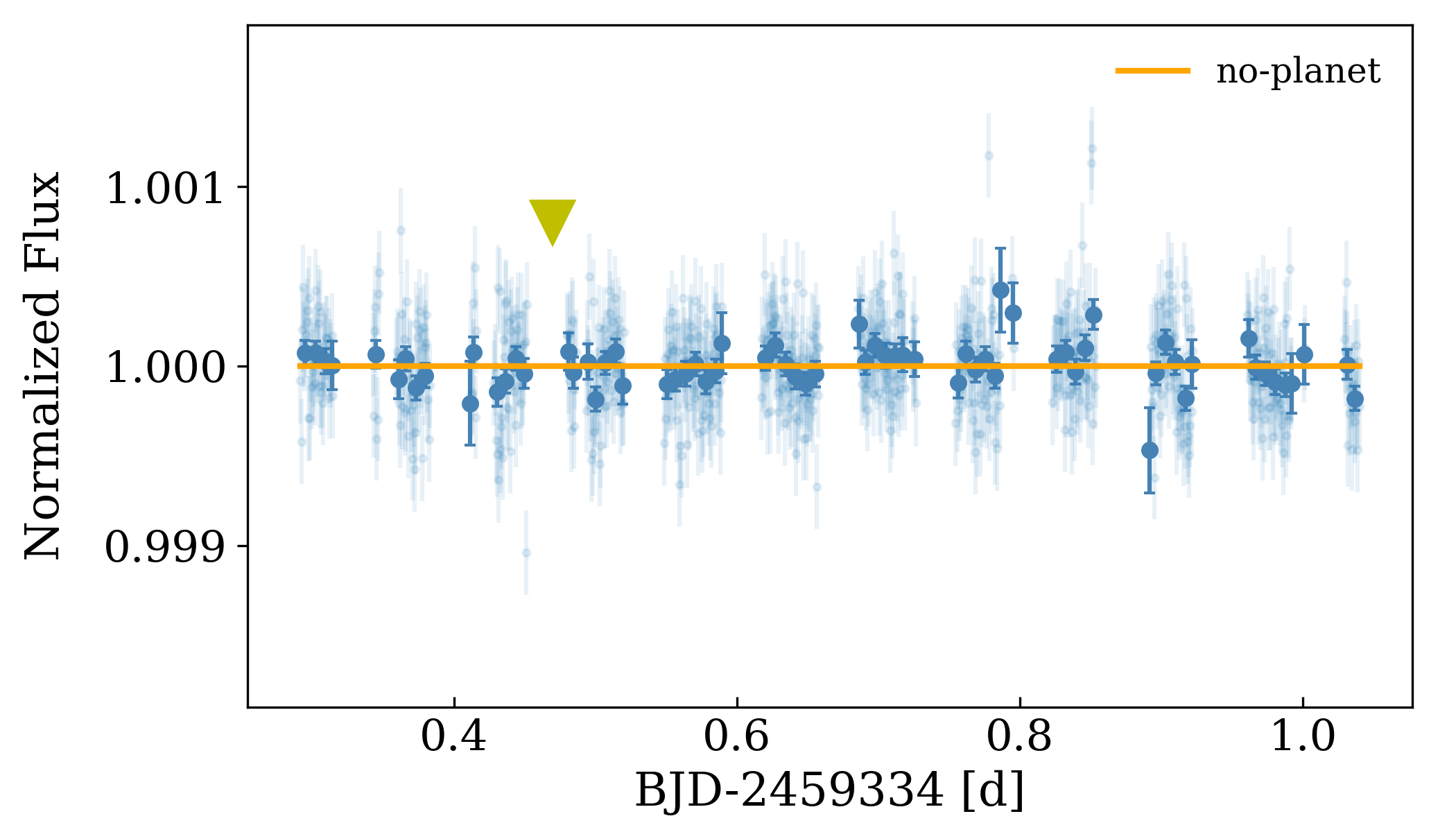
Figure 4: CHEOPS light curves of HD 108236 during the expected transit time of a potential planet $g$ (marked with the yellow triangle). These light curves correspond to observations 1, 9, and 15 in Table 3 (top-to-bottom). Light and dark blue dots represent the detrended and 10 min bins photometric points. No significant statistical evidence of a transit signal with $\sim$10.9 d period is found in these photometric time series.

5 Timing analysis

To perform a detailed timing analysis for each planet, we used the results of the combined analysis in order to determine the transit times for each individual transit event. Therefore, in this case we do not fit for a global P and T₀ for each planet but for the central time, T${}_{\text{c}}$, of each transit event. Thus, we used as priors the results of the combined fit for all the parameters except for the single transit midtime. With these transit times and the ephemeris (described in Sect. 4 and displayed in Table 4) from the global fit, we generated the observed-minus-calculated (O$-$C) diagrams of the five planets in the system. A first analysis showed us that the times of the transits derived from overlapping transit events in TESS light curves correspond to large outliers in the O$-$C diagrams. Thus, for such light curves, we re-fit the two respective planets simultaneously. In this way, we were able to considerably reduce the temporal offsets and the uncertainties of the central times of these transits. The resulting individual transit times are reported in Tables 9 and 10.

We checked if we were able to fit a linear function to the timing residuals of each planet, meaning the ephemeris equation can potentially be updated. We evaluate the significance of the P or T₀ offsets by comparing them with their uncertainties from the global fit. No correction was needed for the orbital periods. We only found significant temporal offsets of 114.5 s (2 $\sigma$), -58 s (1.1$\sigma$) and 717 s (5.9$\sigma$) for the T₀ of planets $b$, $d$ and $f$, respectively. Therefore, we updated the T₀ values of the ephemeris equation for these three planets (Table 5). For comparison, in Table 5 we also show the mean error of the transit times, $\bar{\sigma}_{\texttt{T}_{\texttt{C}}}$, for CHEOPS and TESS transits. The improvement on our estimations of the transit times from CHEOPS light curves in comparison to those from TESS transits is consistent with the results of previous works (e.g., Borsato et al., 2021; Bonfanti et al., 2021). The final O$-$C diagram of each planet is shown in Fig. 5. There, the overlapped transits are marked with the vertical dashed lines, and the $\pm$1-2$\sigma$ uncertainties of the final ephemeris are represented by the gray regions in the diagrams. We noticed non-negligible variations on the transit times of planets $b$ and $f$, reflected for example on the rms and mean amplitude values of their O$-$C residuals. We also noticed hints of an anticorrelation in the transit times of planets $e$ and $f$. Thus, in order to investigate further on the results in the transit times, we performed a detailed transit time variations (TTVs) analysis of the system, described in Sect. 6.3.

Table 5: Results of the timing analysis of the transits.

Planet	O$-$C rms	O$-$C mean	$\bar{\sigma}_{\mathrm{T}_{\mathrm{C}}}^{\mathrm{CHEOPS}}$	$\bar{\sigma}_{\mathrm{T}_{\mathrm{C}}}^{\mathrm{TESS}}$	Updated T0
	[min]	amplitude [min]	[min]	[min]	[BJDTDB - 2 450 000]
$b$	9.6	8.0	3.6	6.6	8572.11149 $\pm$ 0.00065
$c$	4.6	3.4	2.0	3.3	–
$d$	2.4	2.0	4.0	3.1	8571.33610 $\pm$ 0.00060
$e$	2.4	2.4	1.0	2.1	–
$f$	12.6	17.8	4.5	8.8	8616.0486 $\pm$ 0.0014

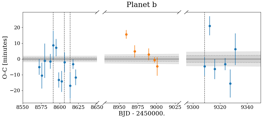
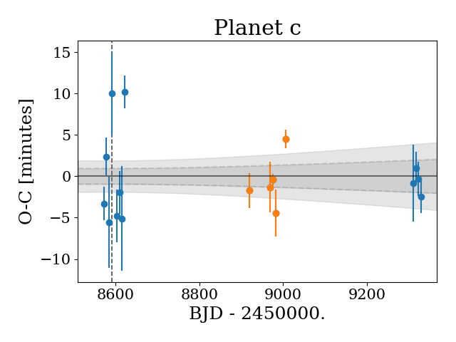
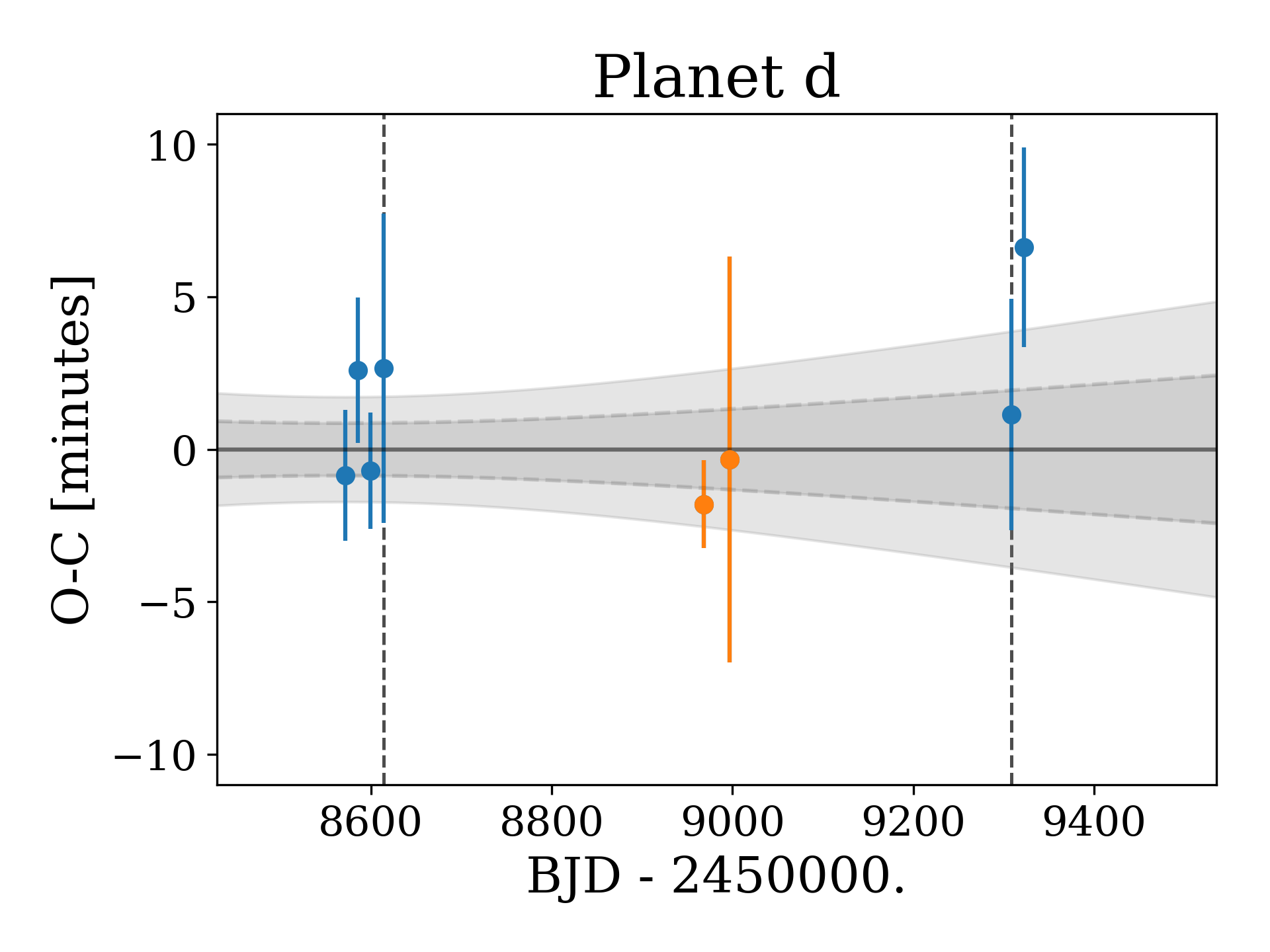
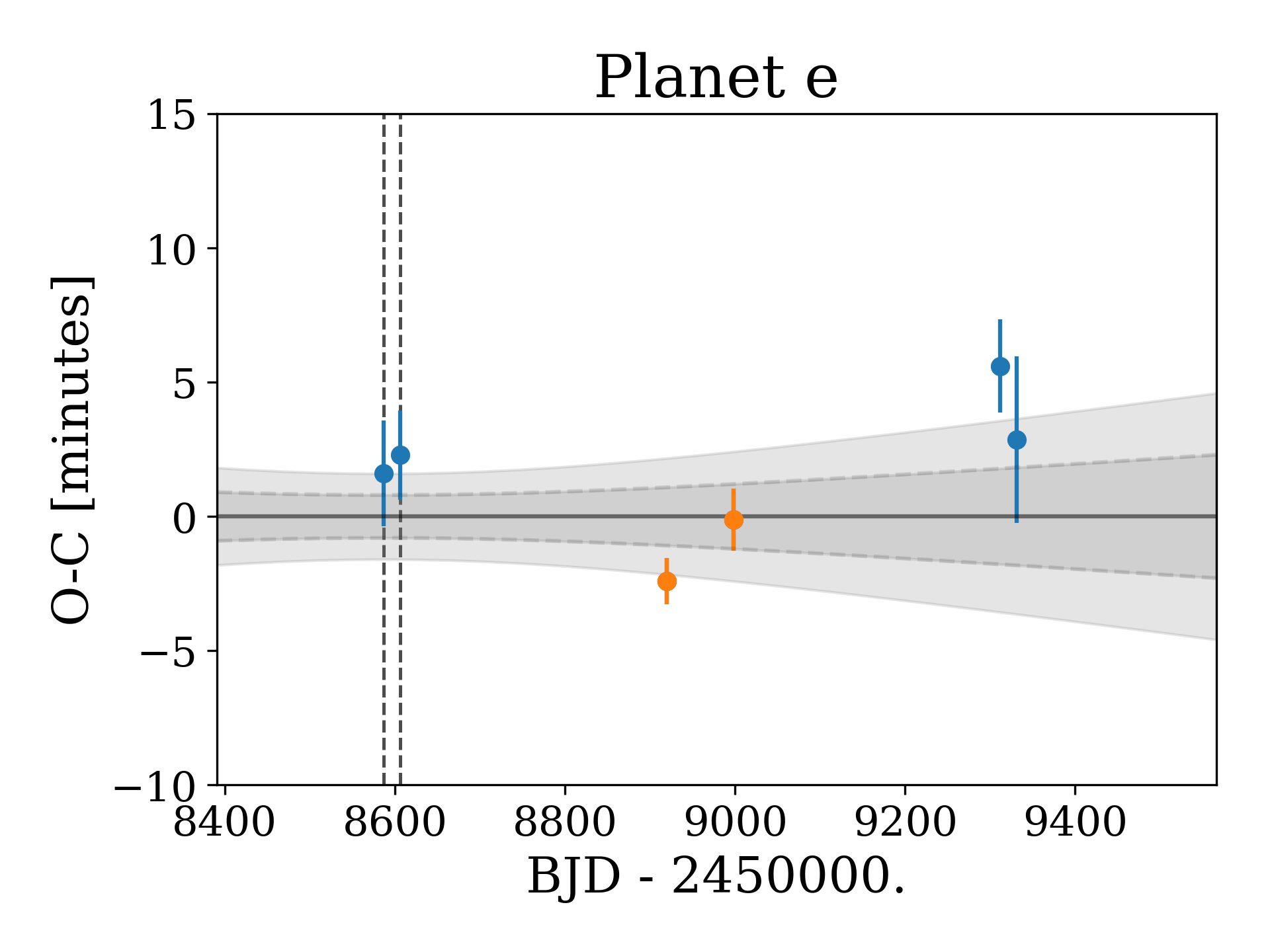
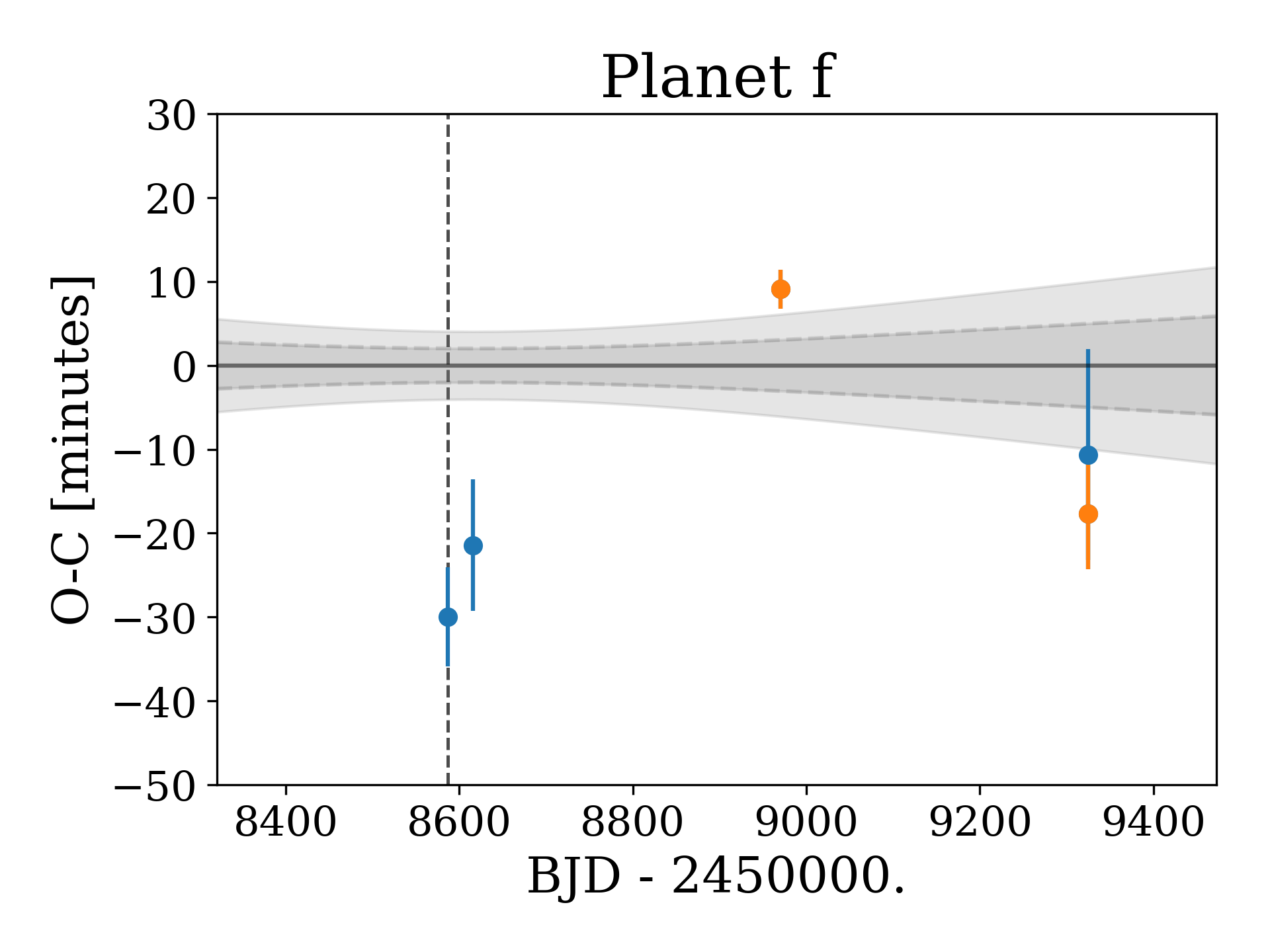
Figure 5: Observed minus calculated diagrams of the transit times of the five planets of the HD 108236 system, obtained by using the ephemeris of the global fit or the updated T₀ values reported in Table 5. Transit times were obtained from the individual analysis of the transits (see Sect. 4). Blue and orange symbols correspond, respectively, to TESS and CHEOPS observations. The gray regions represent the $\pm$1-2$\sigma$ uncertainties of the ephemeris equations. Vertical dashed lines mark overlapped transits in the light curves.

6 Planetary masses

In the absence of radial velocity (RV) measurements, model-dependent estimates of the planetary masses have been previously delivered by Daylan et al. (2021) and Bonfanti et al. (2021). Later, Teske et al. (2021) presented 33 RVs measurements obtained with the Planet Finder Spectrograph (PFS) on the Magellan II telescope at Las Campanas Observatory (Chile). They performed the first Keplerian mass estimation of the HD 108236 system. Among their results for this particular system, it is worth mentioning that they were only able to set an upper limit for the mass of planet $d$ and they predicted an eccentricity of $\sim$0.39 for planet $e$. Here, we take advantage of the refined parameters of the system to estimate the masses of the five planets by, first, performing a new fit of the RV data and; in addition, by using the M-R relations of Chen & Kipping (2017) (CK17 hereafter). Finally, we present our TTV analysis based on the transit timing information of Sect. 5, aimed at exploring whether any constraints can be placed on the planetary masses.

6.1 Radial velocity estimations

For the fitting of the RV observations, we also used juliet, which implements the RADVEL code (Fulton et al., 2018) linked to the dynesty sampler. We set the priors of all the orbital parameters (P_i, T_0,i, $b_{i}$, $e_{i}$ and $\omega_{i}$, $i$:1..5) as normal distributions defined by the results of the photometric fit. For the five RV semi-amplitudes, $K_{i}$, we set a wide uniform prior between 0-20 $m$ $s^{-1}$. We also fit for a jitter and a systemic RV term ($\sigma\_$PFS2 and $\mu\_$PFS2, respectively). The fitted $K$’s and the derived masses for each planet are presented in Table 8, where we also show the masses estimations from the literature. The RV data and the best fitted models are presented in Fig. 16 and 17. Due to the paucity and poor sampling of the observations, the RV masses should be taken with caution, and therefore we treated them as only indicative values. It is known that the accurate measurement of masses of small planets in multiple systems requires considerable large amount of data points (e.g., He et al., 2021), which is not the case of the HD 108236 system to date. In fact, the posterior distribution of the RV semi-amplitude for planet $d$, $K_{d}$, peaks around $K_{d}\sim 0.41$ $m$ $s^{-1}$ (see Fig. 18). As noted in Teske et al. (2021), if we allow a fitting for $K<0$ values, we then would obtain a negative-$K$ ($K_{d}\sim-0.8$ $m$ $s^{-1}$). This was the reason why Teske et al. (2021) adopted only an upper limit for $K_{d}$ defined by the root-mean-square (rms) of the RV residuals after removing the best Keplerian model of the other four planets. We confirmed that the results of the other planets were almost unaffected by removing planet $d$ from the fit. Therefore, we emphasize that our reported RV result for planet $d$ is not reliable.

6.2 Statistical estimations

To compare the RV masses with the values derived with a statistical approach, we use the CK17 M-R relations, implemented within the Python probabilistic tool forecaster. We used as input the derived planetary radius (and its uncertainties) of the five planets obtained from our photometric fit. The masses predicted by CK17 and their uncertainties are presented in Table 8. We also checked that these values are consistent with the predictions from more recent M-R relations from Otegi et al. (2020), although the uncertainties of the later are 2.3-2.7 times smaller. As these M-R relations are intended to provide a broad estimation of the planetary masses, the values we derived with them should be taken with caution.

We note that for the outer two planets, the RV derived masses are unrealistically high when compared to the models outcomes, particularly for planet $f$. This can likely be explained by the fact that the phase of planet $f$ is not well sampled by the RV measurements, and that the fit of planet $e$ seems to show a phase offset, likely resulting in the poor mass determination. Since these two planets are located close to a mutual 3:2 mean motion resonance (MMR), it is possible to explore whether the dynamical analysis can provide additional constraints on the mass estimates, as described in Sect. 6.3.

Table 6: Mass estimations of the planets of HD 108236.

		This work			Literature
Planet	CK17	RVs			T21 (RVs)	B21	D21 (CK17)
	Mass	$K$	Mass	Density	Mass
	[M⊕]	[m s-1]	[M⊕]	[gr cm-3]	[M⊕]
$b$	$3.8^{+2.6}_{-1.3}$	$1.63^{+0.74}_{-0.72}$	$3.6^{+1.7}_{-1.6}$	5.0$\pm$ 2.0	4.33 $\pm$ 1.54	4.23 $\pm$ 0.40	5$\pm$2
$c$	$5.5^{+4.0}_{-2.2}$	$1.94^{+0.79}_{-0.70}$	$5.1^{+2.1}_{-1.8}$	3.0$\pm$1.0	3.97 $\pm$ 1.77	8.90 $\pm$ 0.66	7$\pm$2
$d$	$7.3^{+5.6}_{-3.0}$	$0.46^{+0.54}_{-0.31}$	$1.6^{+1.8}_{-1.1}$	0.5$\pm$0.5	¡7.75	7.75 $\pm$ 0.80	10$\pm$2
$e$	$9.9^{+7.4}_{-4.3}$	$3.55^{+0.78}_{-0.76}$	$13.6^{+3.0}_{-2.9}$	3.0$\pm$1.0	19.10 $\pm$ 3.91	$8.2^{+3.8}_{-1.2}$	13$\pm$2
$f$	$5.1^{+3.8}_{-2.0}$	$4.2^{+1.8}_{-1.6}$	$18.4^{+7.9}_{-7.1}$	15.0$\pm$6.0	10.85 $\pm$ 5.55	3.95 $\pm$ 0.4	–

6.3 TTV Analysis

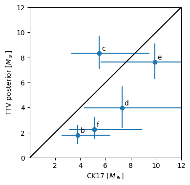
Figure 6: Mass posterior vs. mass prior of the TTV analysis. The error bars show the 1-$\sigma$ interval.

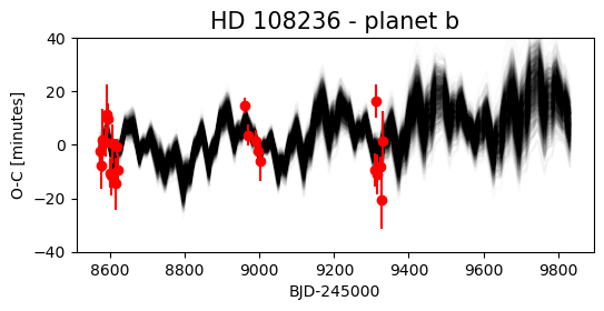
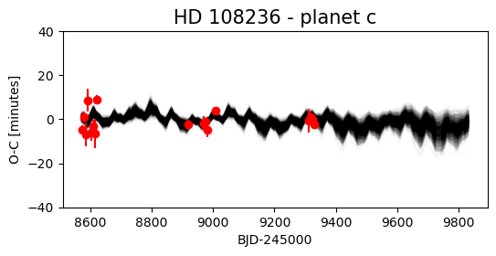
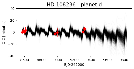
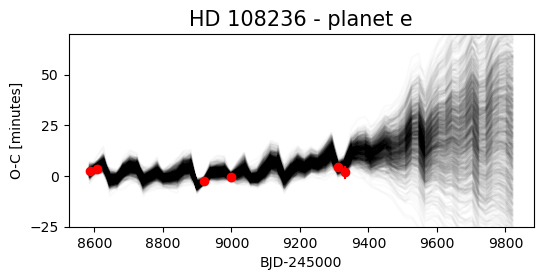
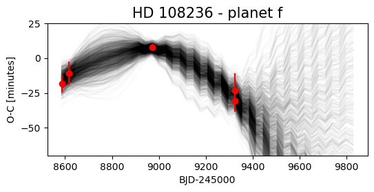
Figure 7: Posterior of the transit timings fit presented in Tables 9 and 10.

The period ratio between consecutive pairs of planets (P_i+1/P_i) in the HD 108236 system is (P${}_{c}/$P_b, P${}_{d}/$P_c, P${}_{e}/$P_d, P${}_{f}/$P_e) = (1.634, 2.285, 1.382, 1.508). Thus, the outer planets, $f$ and $e$, are close to the exact 3/2 commensurability (P${}_{f}/$P${}_{e}\approx 1.508$). The proximity to a two-body mean motion resonances (MMRs), $P_{out}/P_{in}\sim(p+q)/p$, with p and q integers, can generate TTVs that can be observed and modeled to constrain the orbit and masses of the involved planets (e.g., Agol et al., 2005; Lithwick et al., 2012; Nesvorný & Vokrouhlický, 2016). We do not currently have enough TTVs measurement to estimate masses. Here, we report the mass posterior of this TTV analysis with the sole purpose to compare them with the CK17 masses from Table 8 (that we use as prior) in order to check whether these masses are consistent with the observed TTVs.

We fit the timings reported in Tables 9 and 10 using the code presented in Leleu et al. (2021b): the transit timings are estimated using the TTVfast algorithm (Deck et al., 2014), and the samsam MCMC algorithm (see Delisle et al., 2018) is used to sample the posterior. The mean longitudes, periods, arguments of periastron and eccentricities of the planets have flat priors. The masses and eccentricities posteriors of the TTV analysis are shown in Table 8, and 1000 randomly chosen samples of the fitted model are shown in Fig. 7.

The prior-posterior comparison is made in Fig. 6. For planets $b$, $d$, $e,$ and $f$, we see that the mass posterior points toward a lower value than the prior, although the difference lies close to (or within) the 1-$\sigma$ interval. Planet $c$ is the only one for which TTVs mass is larger than the prior, which appears to be due to the tentative chopping in the TTV signal of planet $b$ (see Fig. 7).

For the outer two, near-resonant planets $e$ and $f$, there are hints of anti-correlated TTVs, which are also apparently not fully consistent with the mass priors. For the derived set of masses, significant TTVs are nonetheless expected to come in the next years for these two planets, as can be seen on the TTV projections in Fig. 7 at dates 9600 [BJD-2 450 000] onward. Overall, the TTVs observed for HD 108236 seem to be somewhat at odds with the expected masses and eccentricities, although the current phase coverage is not sufficient to draw strong conclusions and warrant additional observations.

In addition, in order to better constrain the architecture of the system, we used the TTVs posterior to check if the planets $e$ and $f$ are inside the 3:2 MMR using the Hamiltonian formulation of the second fundamental model for Resonance of Henrard & Lemaitre (1983). We applied the ”one degree of freedom” model of first-order resonances presented in Deck et al. (2013), and computed the value of the Hamiltonian parameter $\Gamma^{\prime}$ over the posterior of the TTV analysis (Eq. 36 in the aforementioned paper). The resonant state appears for $\Gamma^{\prime}\geq 1.5$ (Deck et al., 2013), and for this pair of planets ($e$ and $f$) we calculated $\Gamma^{\prime}=-2.76\pm 0.38$, implying that the planets are outside the 3:2 MMR.

7 Discussion

7.1 Planetary parameters

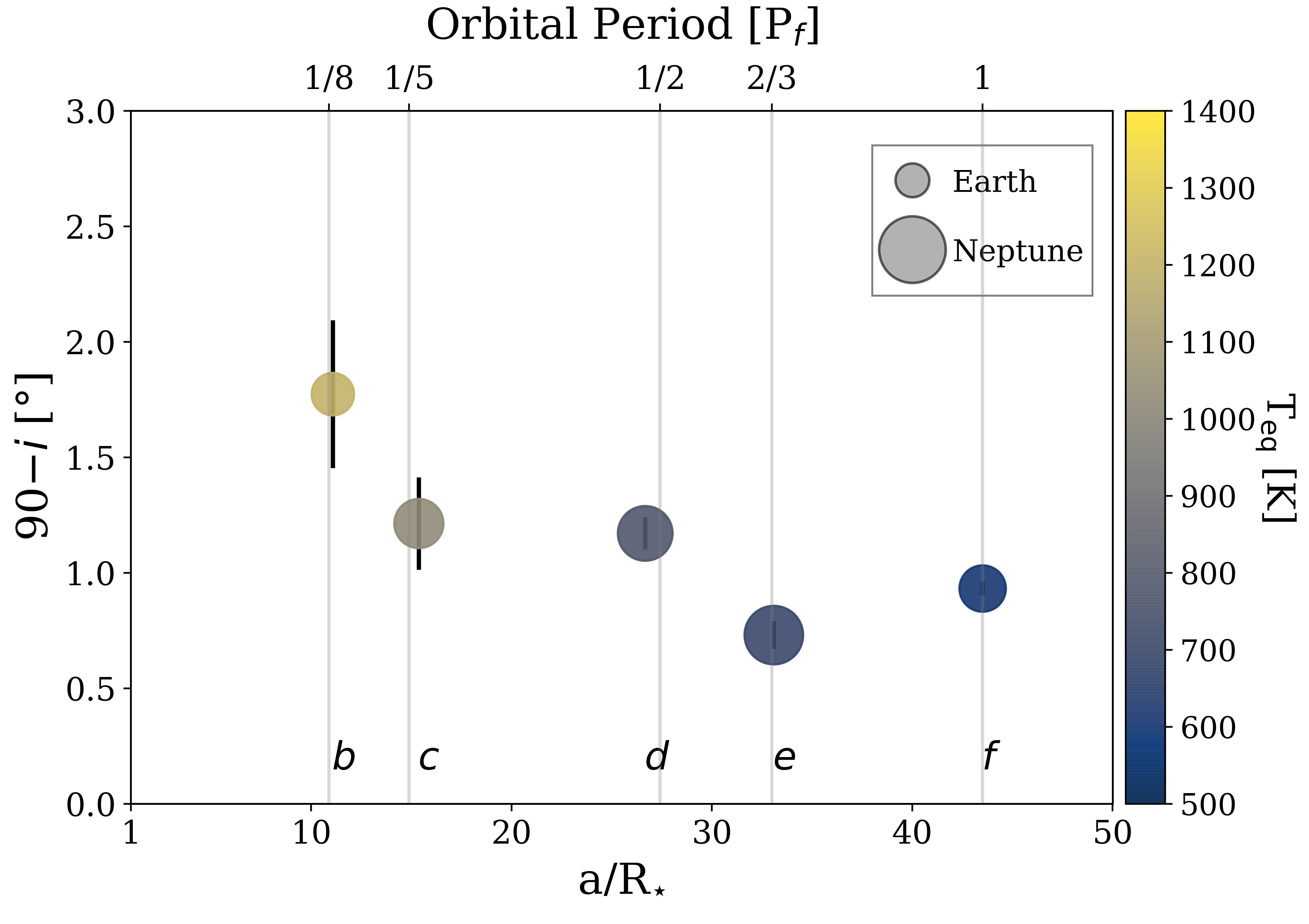
Figure 8: Diagram of the HD 108236 system. We show the scaled semi-major axis, a/$R_{\star}$ (bottom axis) and the respective orbital period of the planets (in units of planet $f$’s period, top axis). We mark the relevant main mean motion resonances with vertical lines. The relative orbital inclination (90${}^{\circ}-i$) of each planet is shown in the left axis. The symbol size scales with the planetary radius in units of Earth radius; and the color with the equilibrium temperature of the planet (with $A_{B}=0$).

As our final planetary parameters, we adopted those resulting from the combined analysis of CHEOPS and TESS data described in Sect. 4 and reported in Table 4. All the parameters are consistent with those presented in Bonfanti et al. (2021) within 1-2$\sigma$. Notably, the uncertainties we report, which represent the 68$\%$ intervals of the resulting posterior distributions of each parameter, are reduced between 30-80 % with respect to previously published uncertainties. A diagram of the orbital configuration, together with a comparative of the sizes of the planets, is presented in Fig. 8.

The uncertainties on the transit ephemeris also improved when compared to Bonfanti et al. (2021) thanks to the extended baseline of the monitored transits. Moreover, we also performed a transit timing analysis (see Sect. 5), which provided us with the updated final T₀ reported in Table 4 for planets $b$, $d,$ and $f$. For the other planets, we still referred to the values in Table 4.

Despite the fact that none of the three approaches we used to estimate the planetary masses are conclusive, we noticed that (as shown in Table 8) the masses of the three most internal planets are consistent among the different estimations (except for RV mass of planet $d$ as discussed in Sect. 6.1). For the two outer planets, the RV masses seem unrealistically high when compared to the other methods, although they are poorly constrained by the data. Below, we use the RV masses to probe the planetary internal structure.

7.2 Rocky or gaseous planets

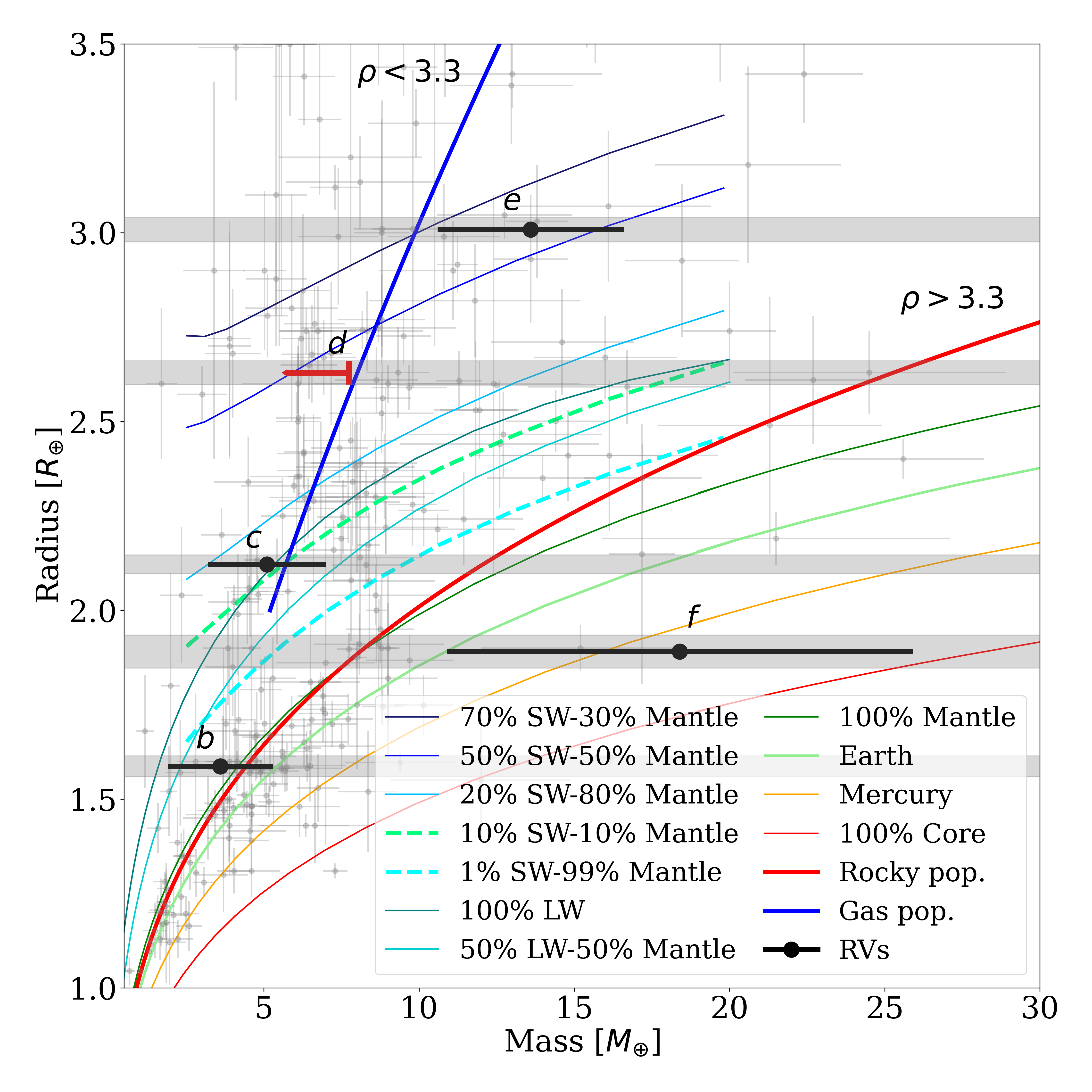
Figure 9: Mass-radius diagram for planets with radius and masses below 3.5 R_⊕ and 30 M_⊕, respectively. The radius of the HD 108236’s planets obtained from the transits modeling are represented by the gray horizontal regions, while the mass values suggested by the RV fit are represented by the black symbols. The upper limit in the mass of planet $d$ (based on estimations from Teske et al. (2021) and Bonfanti et al. (2021)) is marked with the red arrow. We compared the HD 108236 planets with the current planet population (with estimates of mass and radius better than 30%) represented by the gray symbols and the MR relations from Otegi et al. (2020) (blue and red thick lines). The planet interiors models from Brugger et al. (2017) and Acuña et al. (2021) are represented by the thin curves.

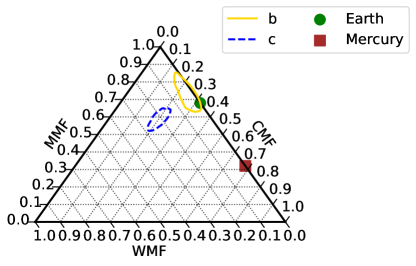
Figure 10: Ternary diagram representing the internal structure of HD 108236 $b$ and $c$, where we show the estimated core mass fraction (CMF), water mass fraction (WMF) and mantle mass fraction (MMF) defined as MMF = 1 $-$ CMF $-$ WMF. The colored contours represent the 1$\sigma$ uncertainties derived from the marginal posterior distribution function for each planet. For comparison, the green dot and red square indicate the position of Earth and Mercury in the ternary diagram, respectively.

Taking advantage of the precision obtained in the planets’ sizes and our RVs estimations of their masses, we placed the five planets of the system in an M-R diagram (Fig. 9). For planet $d,$ we used 7.75 M_⊕ value as an upper limit based on the estimations from Teske et al. (2021) and Bonfanti et al. (2021). We also plotted the M-R relations from Otegi et al. (2020), red and blue thick curves, representing the ”rocky” and ”gaseous” planet populations, respectively. Despite the results of our RV fit are not conclusive, and therefore, the calculated masses and their uncertainties should be treated as indicative values only, we are still able to shed light on the nature of the HD 108236 planets. For this purpose, we overplotted in Fig. 9 the planetary internal models from Brugger et al. (2017) and Acuña et al. (2021). These models consider a planetary interior structure divided in three layers: a Fe-rich core, a silicate mantle and a volatile layer (Brugger et al., 2017). The volatile layer is composed of water, which, depending on the surface pressure and temperature, presents different phases, including liquid, ice, steam, and supercritical. Thus, the models in Fig. 9 represent different ratios of core, mantle and volatile rich envelope with water either in the supercritical (SW) or liquid (LW) form. In the case of the SW mass-radius relationships, we have considered an equilibrium temperature of 1200 K, which is approximately the equilibrium temperature of planets $b$ and $c$.

Thus, based on its location on the M-R diagram, planets $d$ and $e$ likely have a significant volatile envelope surrounding a large mantle. Unfortunately, with the data in hand, for these planets, it is not possible to say anything further about the relative fraction of these two layers. For planet $f$, for which the RVs suggest a rocky composition although the proportion between mantle and core components is not possible to constrain due to the large uncertainties we still have on its mass.

On the contrary, despite their mass uncertainties, it is possible to discriminate between a rocky planet with no volatiles and a volatile-rich planet for planets $b$ and $c$. For these planets, we performed a more detailed interior structure analysis within a MCMC Bayesian framework, as described in Acuña et al. (2021). For this analysis, we considered the masses estimated from the RVs (Table 8) and the radii presented in Table 4. With an equilibrium temperature of about 1200 K, these planets are highly irradiated; therefore, in our interior structure model, we assumed that the volatile layer is not water in a condensed form, but in supercritical and steam phases (Mousis et al., 2020; Acuña et al., 2021). The upper region of the volatile layer consists of an atmosphere in radiative-convective equilibrium that is coupled with the interior at 300 bar. The atmospheric temperature at the bottom of the volatile layer, $T_{300}$, the Bond albedo, and the atmospheric thickness were calculated with a 1D k-correlated model (Pluriel et al., 2019; Marcq et al., 2017). In addition, we also considered the Fe/Si mole ratio as an observable in our MCMC analysis, which is calculated as described in Sotin et al. (2007) and Brugger et al. (2017), using our HD 108236’s abundance estimations of Fe, Si, and Mg (Table 2). We obtain a Fe/Si=0.79$\pm$0.08, which is below the solar value Fe/Si_⊙=0.96 (Sotin et al., 2007). The core mass fraction (CMF), the water mass fraction (WMF), and the atmospheric parameters, resulting from our interior structure analysis, are shown in Table 7.

We found that the densities of all planets in the system can be accounted by a core and a mantle with a Fe/Si mole ratio equal to that of the stellar host, together with a volatile layer on top. Under this assumption, in the Fe/Si mole ratio, planet $b$ could have a thin atmosphere (¡ 300 bar) or an envelope that could constitute up to 10% of its mass. To explore the possibility of planet $b$ being a ”dry” super-Earth, that is, composed of a core and a mantle only, we removed the Fe/Si mole ratio as a constraint in our MCMC Bayesian analysis, leaving only the observable constraints imposed by mass and radius. In addition, we fixed the WMF to zero. In this case, planet $b$ is compatible with a dry planet with CMF=0.04${}^{+0.22}_{-0.04}$ and a Fe/Si = 0.67$\pm$0.54, having a low Fe content compared to the Earth value (CMF_⊕ = 0.32). We observe that planet $c$ is more volatile-rich than planet $b$ (see Table 7 and Fig. 10). On the other hand, it would be necessary to better constrain the masses of planets $d$ and $e$ to narrow down the mean value and uncertainties of their volatile mass fractions. If their volatile contents are confirmed to be higher than that of planet $c$, the HD 108236 system could present an increasing volatile mass fraction trend with increasing semi-major axis, which has been noted in other multi-planetary systems with low-mass planets (e.g., Acuña et al., 2022). In addition, if the rocky nature of planet $f$ is confirmed, for example via a more complete RV follow-up, it would be very interesting to explore the processes in the formation and/or evolution of the system, such a Jeans atmospheric escape, required to explain why the more massive and less irradiated planet does not present a gaseous envelope unlike its two precedent planets.

Table 7: Compositional and atmospheric parameters for HD 108236 planets $b$ and $c$.

Planet	CMF	WMF	$T_{300}$ [K]	$z_{atm}$ [km]	$A_{B}$
$b$	0.24$\pm$0.06	0.05 $\pm$ 0.05	4071$\pm$135	1035$\pm$395	0.22$\pm$0.01
$c$	0.20$\pm$0.02	0.21$\pm$0.05	3804$\pm$123	733$\pm$179	0.22$\pm$0.01

8 Conclusions

In this work, we present the most comprehensive characterization of the HD 108236 system based on the photometric data gathered by CHEOPS and TESS space missions. We confirm the existence of a fifth transiting planet with an orbital period of 29.54 d. On the contrary, we found no indication of transit signals of a putative additional planet in a 10.9 d orbit in CHEOPS dedicated observations we performed. A planet larger than 0.42 R_⊕ (with $e$=$b$=0) would have been detectable in our dataset at S/N=1. The general picture of the HD 108236 system is summarized in Fig. 8.

With our analysis, we greatly improved the characterization of the planetary properties, in particular, we refined the size estimations of the five planets in the system with uncertainties between 1.5–3%. Also, the extensive and detailed timing analysis facilitated an update for the ephemeris of all the planets and to report that TTVs were observed for planets $b$ and $f$. Moreover, in the absence of a profuse RV monitoring to date, we performed mass estimations of the planets by different approaches. As illustrated in Table 8, the best agreement between the different applied methods was obtained for the inner planets. On the other hand, a large spread in the mass estimations is seen for the two outer planets. In this case, the constraints set by the timing analysis for that pair of planets in a 3:2 MMR, suggest a low density configuration for these bodies. A TTV analysis that would include additional transits for these two bodies would allow stronger constraints to be placed on their gravitational interaction and, thus, their density as well as the architecture of the system.

Thanks to its brightness, HD 108236 system is fitting for an intense and precise radial velocity follow-up, which together with our precise estimations of the planetary radii will provide definitive constraints on the density of the transiting bodies.

Based on the refined planetary properties, we computed the transmission spectroscopy metric (TSM) of Kempton et al. (2018) to estimate its suitability for a potential atmospheric follow-up with James Webb Space Telescope (JWST, Gardner et al., 2006). By using the RV masses (Table 8) and the upper limit of planet $d$ (M${}_{d}=7.75\pm 1.0$) from the estimations of Teske et al. (2021) and Bonfanti et al. (2021), we obtained the following TSM values for each planet ($b$ to $f$): 54 $\pm$ 26, 77 $\pm$ 30, 73 $\pm$ 10, 56 $\pm$ 13, and 9 $\pm$ 4, where the errors are dominated by the uncertainties on the planetary mass, with all of them below the suggested threshold for this range of planet sizes (TSM¿90). The potential for an JWST atmospheric follow-up will be finally defined when the densities of these planets are better determined. So far, our analysis suggests the presence of significant atmospheres in planets $c$ to $e$. On the contrary, planet $b$ is compatible with the presence of a thin atmosphere, or a Fe-poor dry planet, while planet $f$ seems to have a rocky structure.

Appendix A Raw and detrended CHEOPS light curves

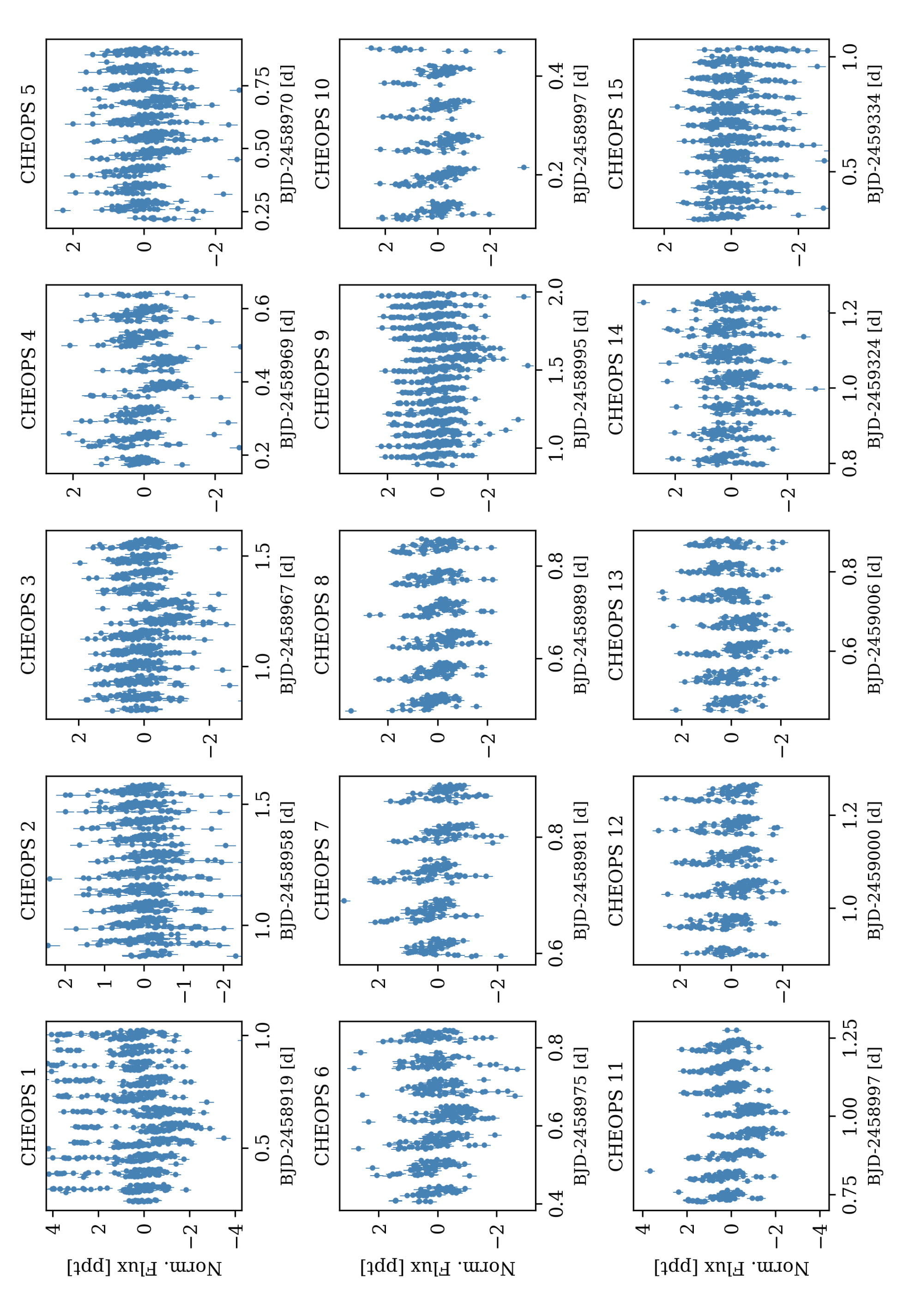
Figure 11: Normalized CHEOPS raw light curves of HD 108236 used in this work. Large outliers have been clipped out to improve visualization. The CHEOPS label number on top of each panel correspond to the ID given in Table 3.

In Fig. 11 we show the raw light curves as output by the CHEOPS Data Reduction Pipeline (DRP-v13, Hoyer et al. 2020). These light curves are usually affected by systematics as a function of the rotation angle of the Field of View along the pointing direction. In Figs. 12 and 13 we show the detrended version of the CHEOPS light curves (see Sect.4.1 for details), together with the best models obtained from the global modeling of the system (Sect. 4).

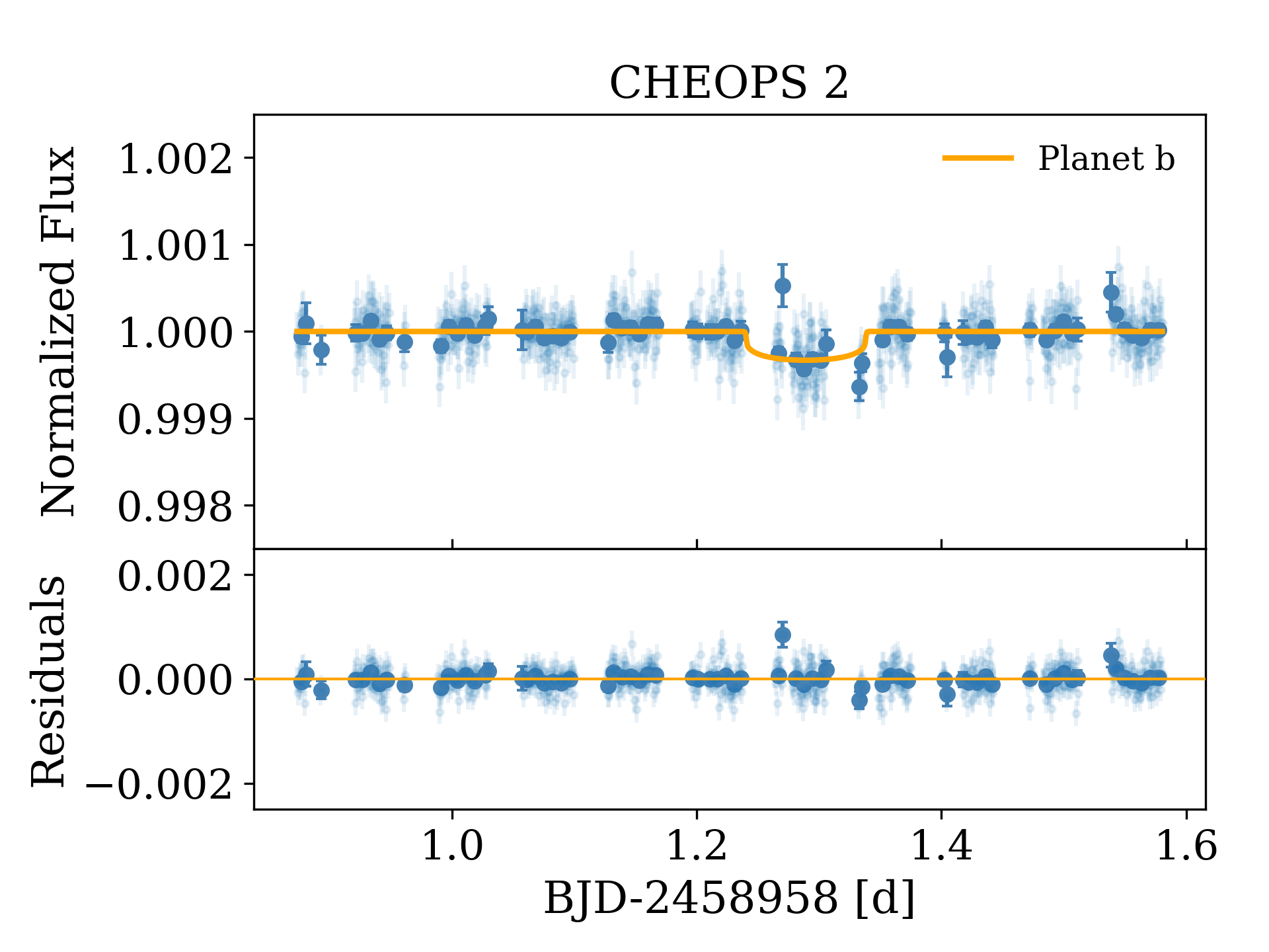
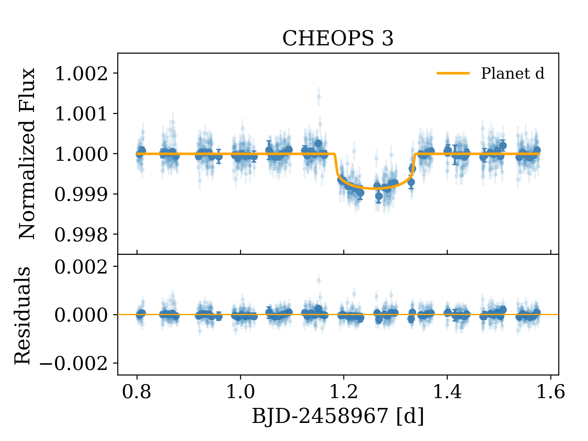
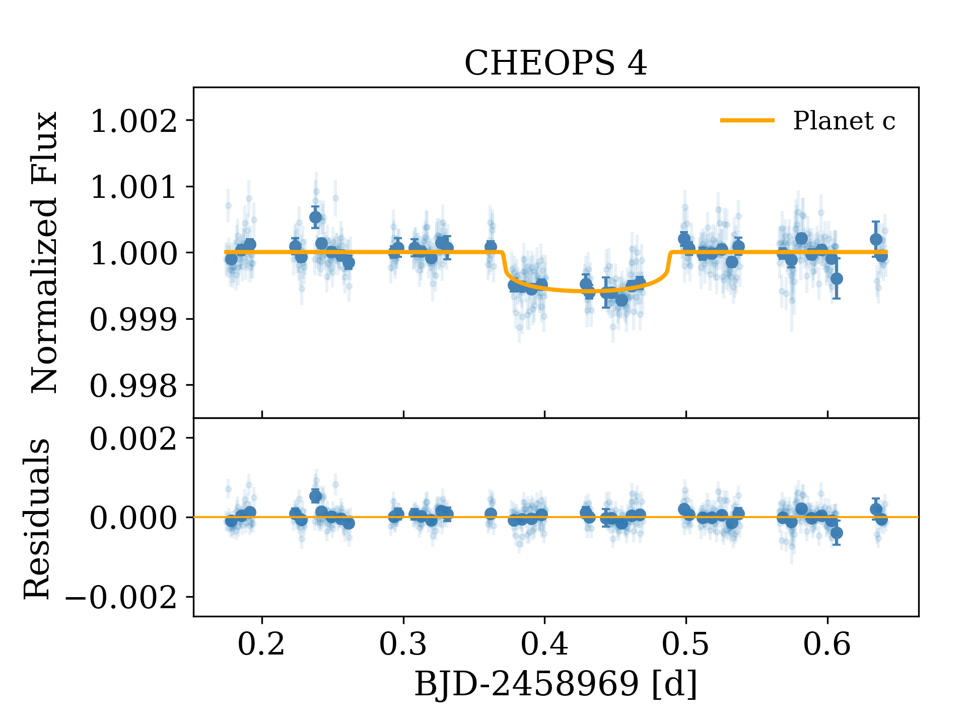
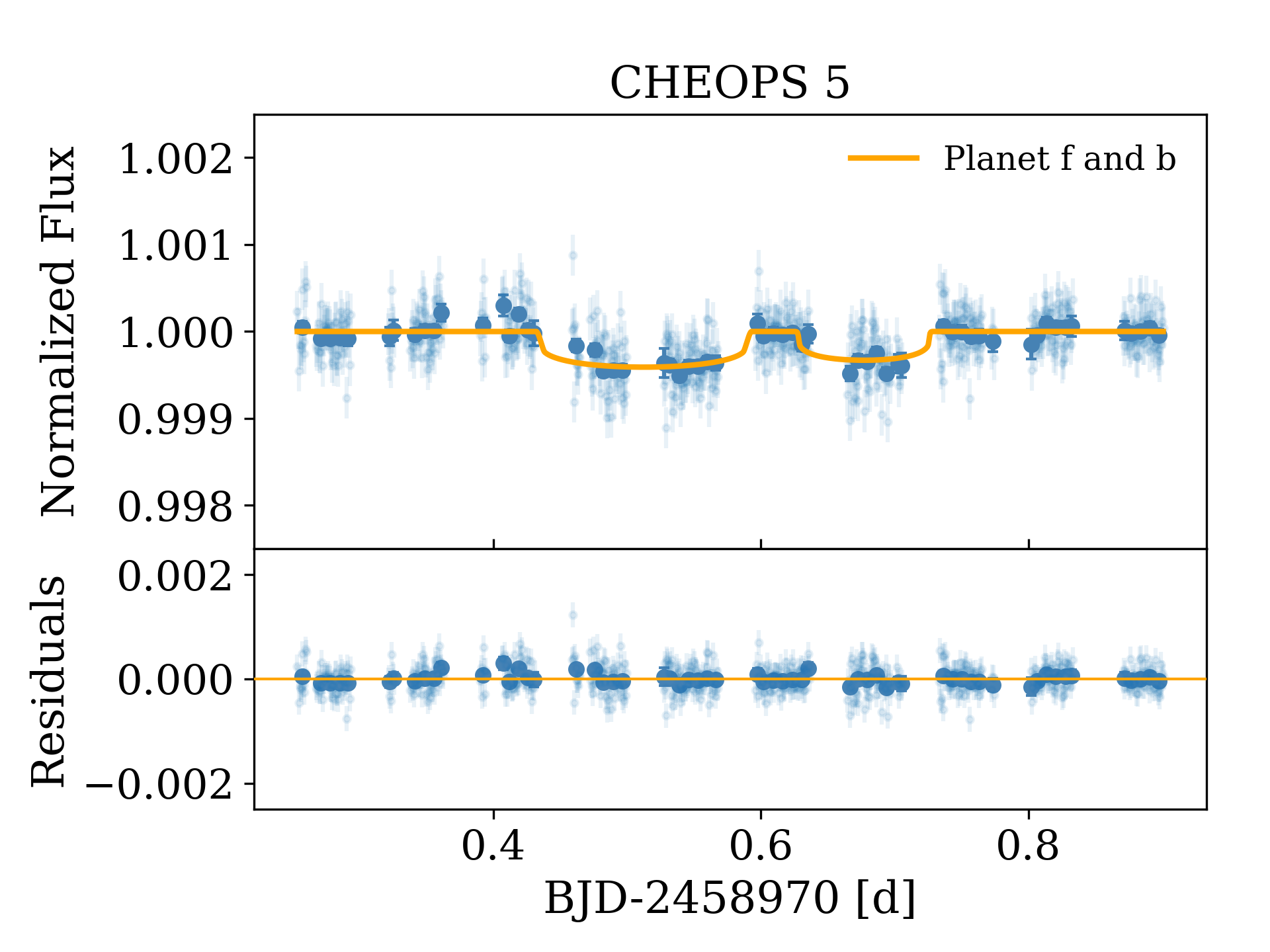
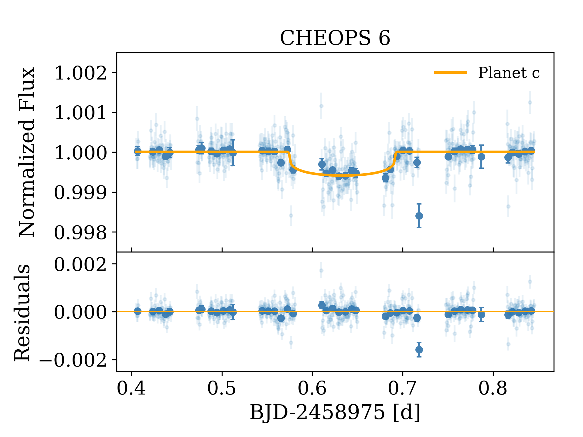
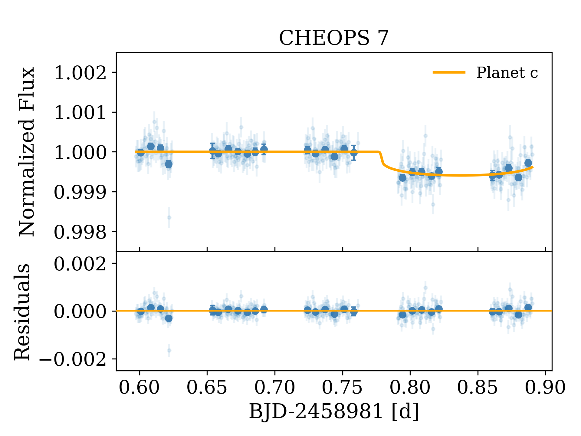
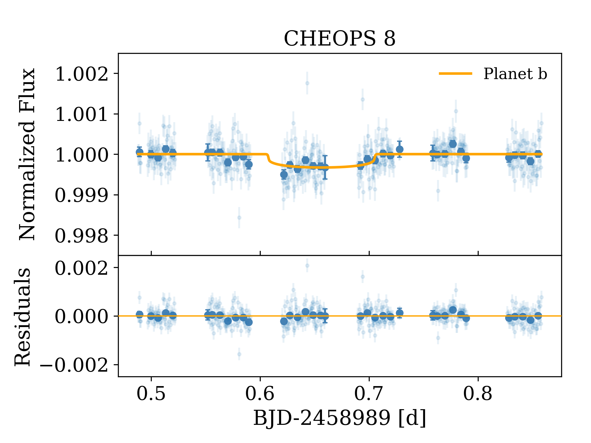
Figure 12: Normalized CHEOPS detrended light curves of HD 108236 used in this work and its 10 min bins are shown, respectively, with light and dark blue symbols. The best transit models obtained from the global analysis of the system are represented by the yellow curve. The residuals are shown in the bottom panels.

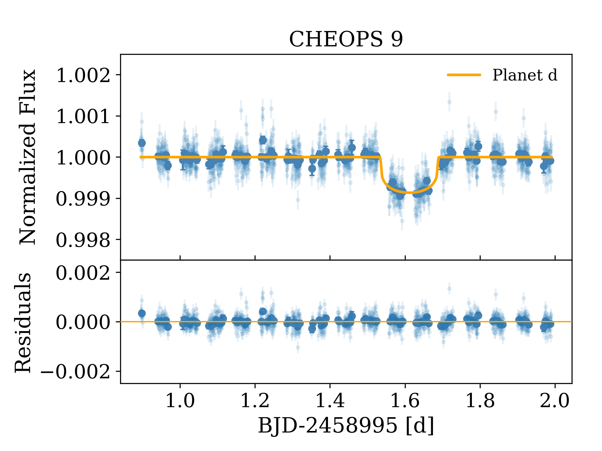
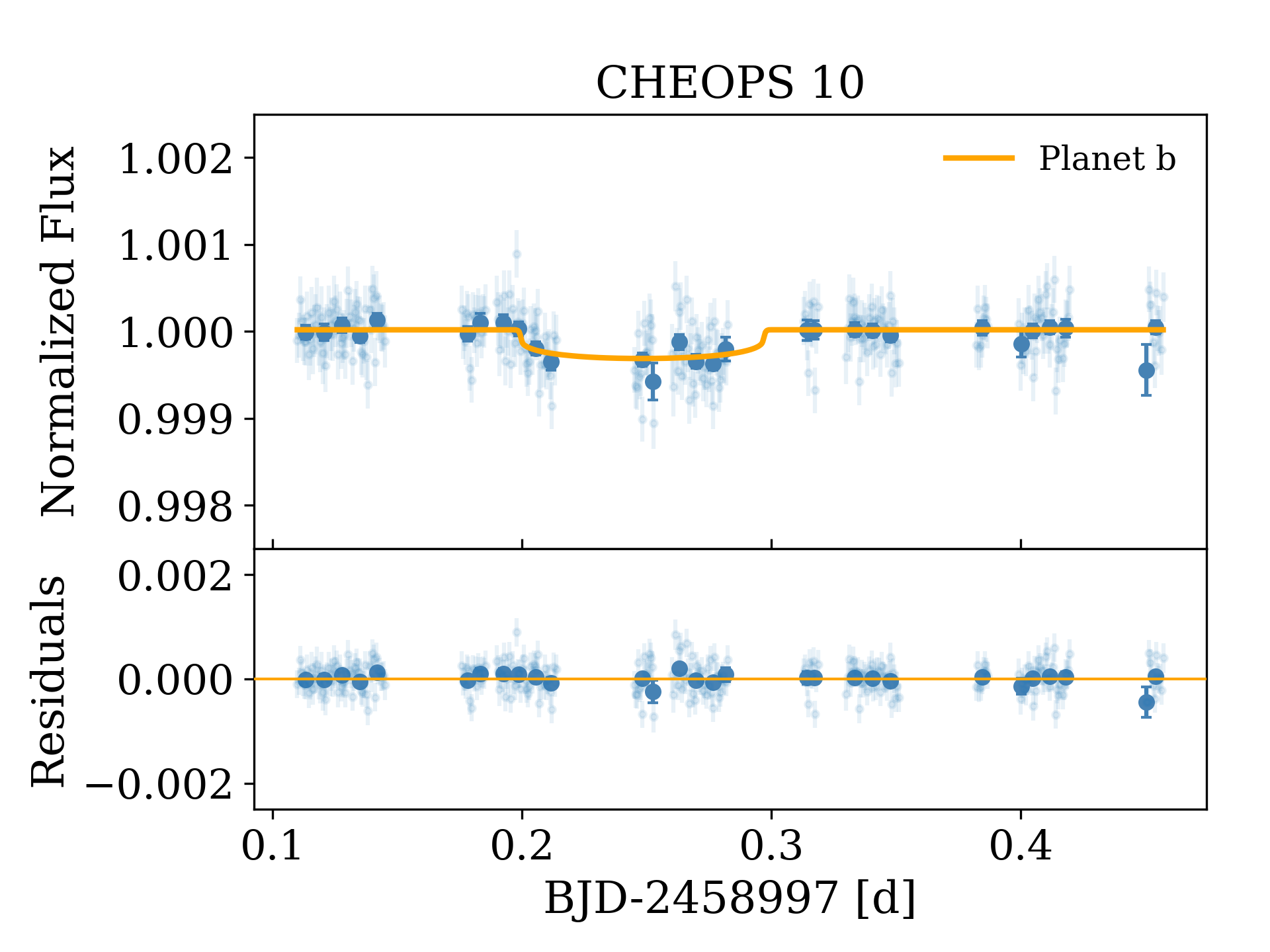
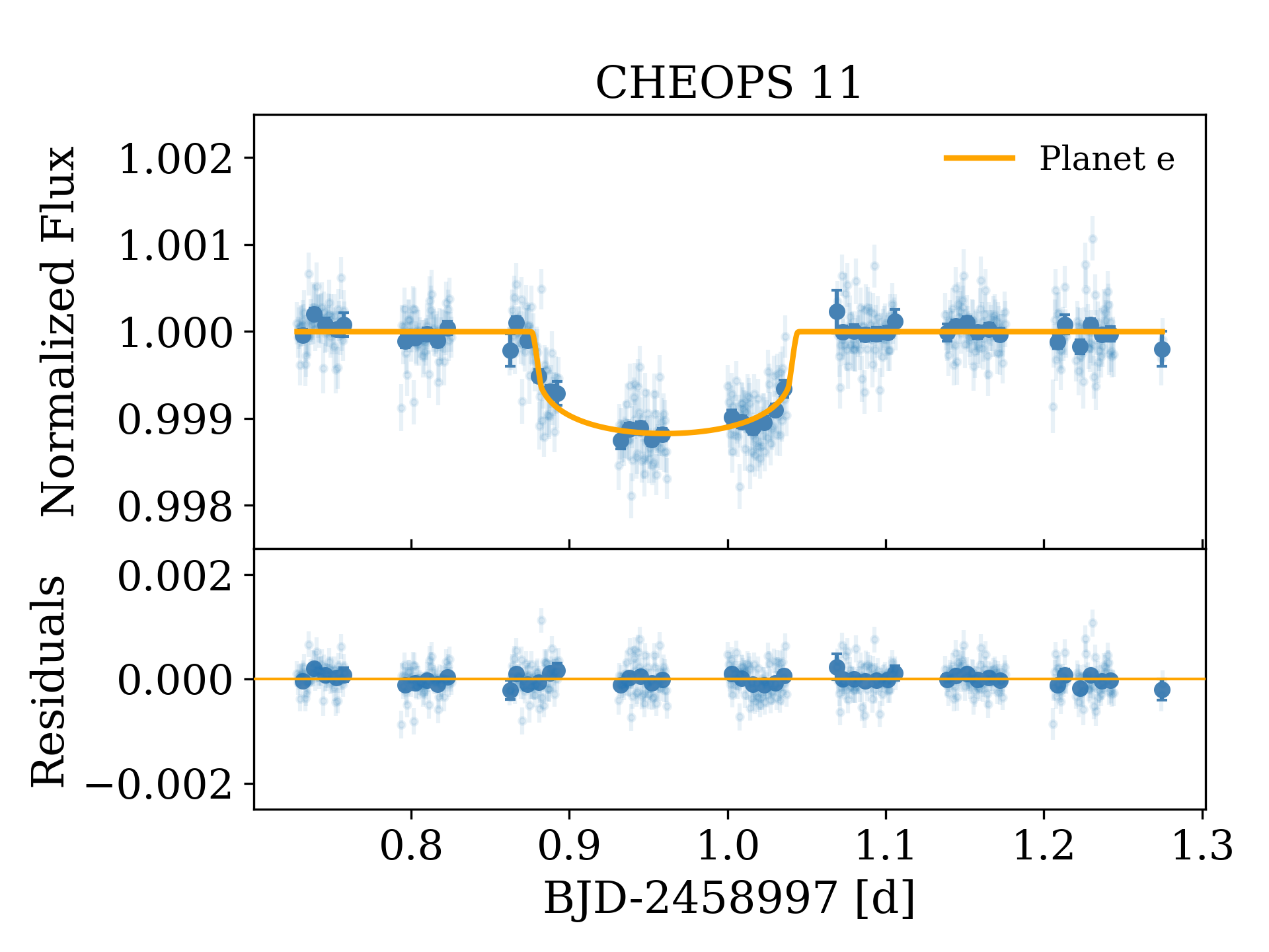
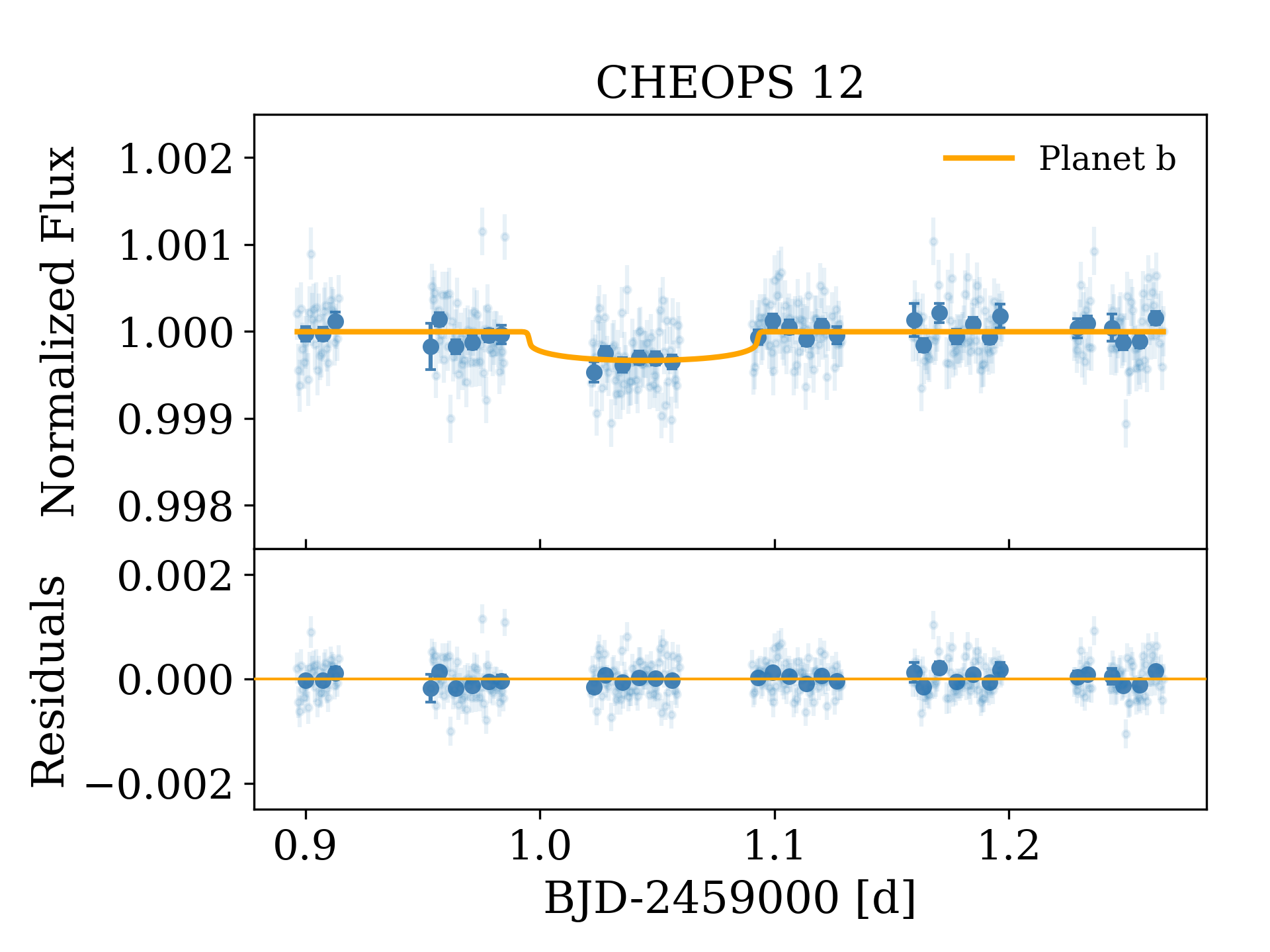
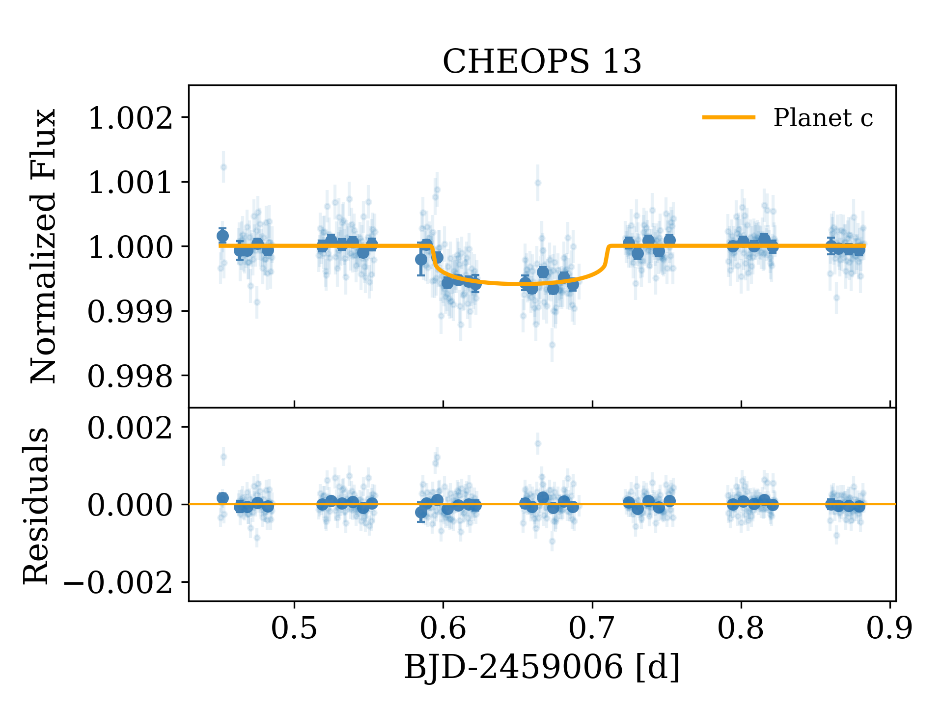
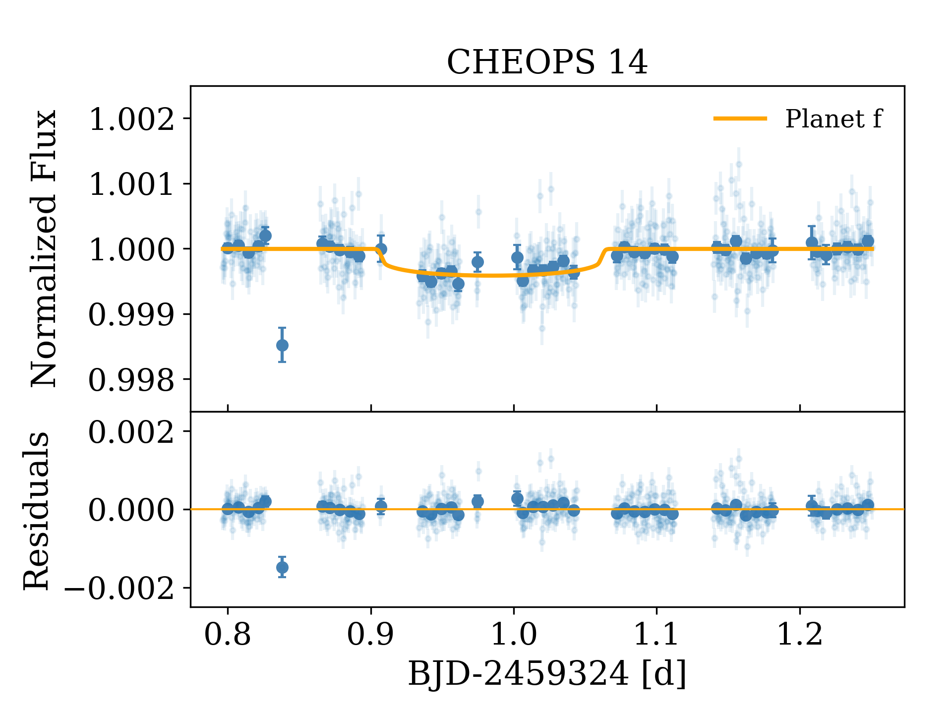
Figure 13: Normalized CHEOPS detrended light curves of HD 108236 used in this work and its 10 min bins are shown, respectively, with light and dark blue symbols. The best transit models obtained from the global analysis of the system are represented by the yellow curve. The residuals are shown in the bottom panels.

Appendix B Initial priors of the LC analysis

In Table 8, we list the priors distributions used for the global fit of all the photometric data described in Sect. 4, consisting of 34 TESS and 15 CHEOPS light curves.

Table 8: Priors for each of the parameters fitted in the global photometric analysis of CHEOPS and TESS data.

Parameter	Prior
Star
$\rho_{\star}$ [$kg$ $m^{-3}$]	$\mathcal{TN}(1790,110,1680,1900)$
$q_{1,{\mathrm{TESS}}}$	$\mathcal{N}(0.34,0.05)$
$q_{2,{\mathrm{TESS}}}$	$\mathcal{N}(0.27,0.05)$
$q_{1,{\mathrm{CHEOPS}}}$	$\mathcal{N}(0.46,0.05)$
$q_{2,{\mathrm{CHEOPS}}}$	$\mathcal{N}(0.32,0.05)$
Planet $b$
$R_{p}/R_{\star}$	$\mathcal{N}(0.01688,0.01)$
T0-2 450 000. [BJD]	$\mathcal{N}(8572.1128,0.01)$
P [$d$]	$\mathcal{N}(3.796,0.001)$
Planet c
$R_{p}/R_{\star}$	$\mathcal{N}(0.0217,0.01)$
T0-2 450 000. [BJD]	$\mathcal{N}(8572.3949,0.01)$
P [$d$]	$\mathcal{N}(6.203,0.001)$
Planet d
$R_{p}/R_{\star}$	$\mathcal{N}(0.0266,0.01)$
T0-2 450 000. [BJD]	$\mathcal{N}(8571.3368,0.01)$
P [$d$]	$\mathcal{N}(14.1758,0.001)$
Planet e
$R_{p}/R_{\star}$	$\mathcal{N}(0.0322,0.01)$
T0-2 450 000. [BJD]	$\mathcal{N}(8586.5677,0.01)$
P [$d$]	$\mathcal{N}(19.59,0.001)$
Planet f
$R_{p}/R_{\star}$	$\mathcal{N}(0.0211,0.01)$
T0-2 450 000. [BJD]	$\mathcal{N}(8616.039,0.01)$
P [$d$]	$\mathcal{N}(29.5398,0.001)$
All planets
$b$ [$R_{\star}$]	$\mathcal{U}(0.001,0.99)$
$\sqrt{e}sin(\omega)$	$\mathcal{U}(-0.3,0.3)$
$\sqrt{e}cos(\omega)$	$\mathcal{U}(-0.3,0.3)$
Instrumental
$mflux\_\small{\texttt{TESS}_{i}}$	$\mathcal{N}(0.0,0.1)$
$\sigma_{w}\_\small{\texttt{TESS}_{i}}$ [ppm]	$log\mathcal{U}(0.1,1000)$
$mflux\_\small{\texttt{CHEOPS}_{i}}$	$\mathcal{N}(0.0,0.1)$
$\sigma_{w}\_\small{\texttt{CHEOPS}_{i}}$ [ppm]	$log\mathcal{U}(0.1,1000)$
$c_{1}(t)_{\_}\small{\texttt{CHEOPS}_{i}}$	$\mathcal{U}(-1.0,1.0)$
$c_{2}(t^{2})_{\_}\small{\texttt{CHEOPS}_{i}}$	$\mathcal{U}(-1.0,1.0)$

Appendix C Role of the parametrization in the fitted parameters: $e$, $\omega$ and $b$.

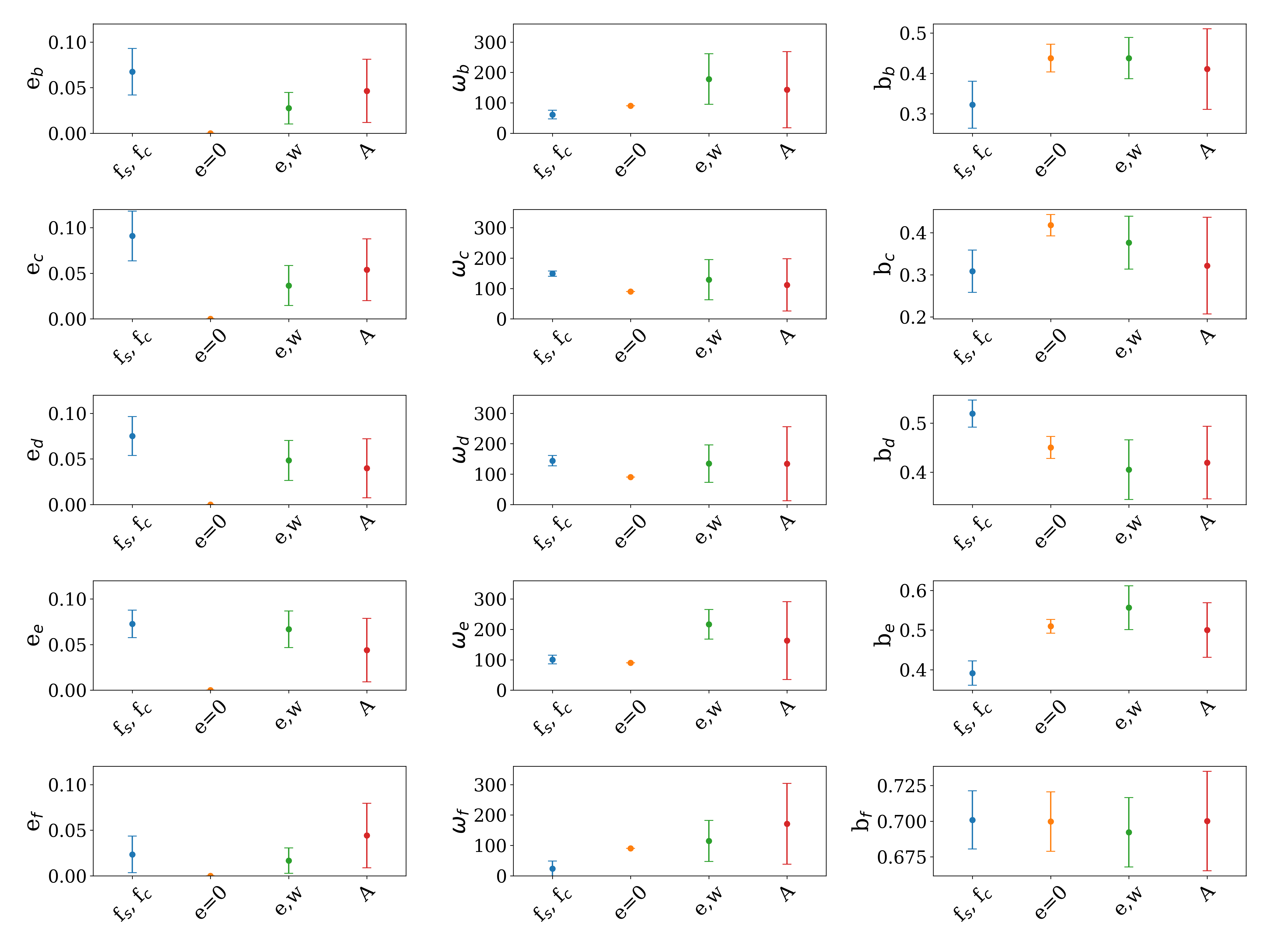
Figure 15: Comparison of fitted values using different parameterizations/priors. We show the fitted eccentricity, $e$ (left panels), argument of periastron $\omega$ (middle panels), and impact parameter $b$ (right panels) of each planet. In the x-axis we denote the used method: the (f_s,f_c) parametrization, fixing the eccentricity to zero ($e=0$) and by jumping directly on $e$ and $\omega$ ($e$,$\omega$). We also show the resulting values of the modeling with Allesfiter code ($A$).

We explored different configurations of the system modeling with juliet to compare the resulting values of the orbits’ eccentricities and any possible effect it might have in other planetary parameters. As described in Sect. 4.2, we used the parametrization f_s = $\sqrt{e}sin(\omega)$ and f_c = $\sqrt{e}cos(\omega)$ to fit for the eccentricity ($e$) and the argument of the periastron ($\omega$). In addition, we performed two extra modelings by either fitting $e$ and $\omega$ directly or assuming $e$=0 and $\omega=90^{\circ}$. The different models were also compared with the fit performed using Allesfiter. We found that, in general, all the fitted parameters were consistent well within 1$\sigma$. The largest differences are found in the eccentricities as illustrated in Fig. 15. We notice that, for planets $b$, $c$ and $d$ the eccentricities derived using (f_s,f_c) parametrization are systematically large in comparison with the other fits. We found that in this case, eccentricities are correlated with the impact parameters, which were also discrepant with the values obtained with the other fits (see right panels in Fig. 15). These differences likely raise because juliet does not fit for $b_{\mathrm{circ}}$ (the impact parameter of the circular orbit, see e.g., Gillon et al. 2009), but for the eccentric $b^{\prime}$, hence producing correlations between $b^{\prime}$ and the resulting $e$ as:

$$b^{\prime}=b_{\mathrm{circ}}(1+e\leavevmode\nobreak\ sin(\omega))/(1-e^{2}).$$ (1)

Allesfitter, instead, assumes (R${}_{p}+$R_s)/$a$ and $cos(i)$ as priors, whose combination essentially gives $b_{\mathrm{circ}}$. Thus, with Allesfitter, we avoided $b^{\prime}$ versus $e$ correlations; we also obtained non-zero eccentricities, but only 1.5$\sigma$ away from the zero (although Allesfitter’s uncertainties are systematically larger). It is also known that fitting directly $e$ and $\omega$ biases towards low eccentricities (e.g Anderson et al. 2011; Eastman et al. 2013), behavior that we also confirm. Therefore, we attribute the larger eccentricities reported in Table 4 to the parametrization used by juliet. We recall the difficulty in obtaining a robust estimate of the orbital eccentricities with photometry of primary transits alone and thus a detailed RV analysis is required for achieving a final conclusion in this regards.

Appendix D Ruling out the putative planet $g$

Confirming the five-planet architecture of the system or preferring the six-planet scenario is an example of model selection problem. Before acquiring the last CHEOPS light curve of the putative planet $g$ (Fig. 4, bottom panel), we compared the two scenarios by performing several pairs of comprehensive analyses, which involved all the other CHEOPS light curves (where planet $g$ is expected to transit twice) and the two TESS sectors, 10 and 11, (where planet $g$ is expected to transit five times). To address the model selection problem, the analyses were performed through the dynamic nested sampling technique (see e.g., Feroz & Hobson 2008; Feroz et al. 2019) implemented in the dynesty package (Speagle 2020) and incorporated in Allesfitter. In fact, dynesty outputs the Bayesian evidence $\mathcal{Z}$ of the adopted model, so that it is then straightforward to decide whether to prefer a more complicated model (e.g., $\mathcal{M}_{1}$) against a simpler one ($\mathcal{M}_{0}$) by computing the Bayes factor $\mathcal{B}_{10}$ as defined in Kass & Raftery (1995):

$$\mathcal{B}_{10}=\frac{\mathcal{Z}_{1}}{\mathcal{Z}_{0}},$$ (2)

where $\mathcal{Z}_{i}$ ($i=0,1$) is the Bayesian evidence of the $i^{\mathrm{th}}$ model. As reported by Kass & Raftery (1995), we recall that a very strong evidence against the null hypothesis (i.e. the more complicated $\mathcal{M}_{1}$ model is accepted) occurs when $\ln{\mathcal{B}}_{10}>5$.

Following a first analysis, where we included only planets from $b$ to $f$ (model $\mathcal{M}_{5}$), we added the putative planet $g$ to our input file, adopting uniform priors in agreement with the guess values from Daylan et al. (2021) (model $\mathcal{M}_{6}$). The code was actually able to model also the sixth planet, but we obtained a transit depth $\delta=127\pm 21$ ppm, which is half the value suggested by Daylan et al. (2021) and $\sim$ 6$\sigma$ away. Moreover, the posterior distributions of P and T₀ have heavy tails, with the uncertainty on T₀ that is one order of magnitude larger than what we found for the other planets. This indicates a poor convergence, probably due to the code attempts of modeling transit-like wiggles. We also looked at the rms of the residuals coming from the five-planet and six-planet analyses (rms₅ and rms₆, respectively), considering whether rms₆ values were statistically lower than rms₅. To this end we applied the Wilcoxon test (Wilcoxon 1945), whose null hypothesis is that the two samples comes from a single population (i.e., they are statistically equal) obtaining $p$-values ¿ 0.79, which provides no evidence for preferring the six-planet scenario. On the other hand, we computed the Bayes factor $\mathcal{B}_{65}$ comparing $\mathcal{M}_{6}$ vs. $\mathcal{M}_{5}$ obtaining $\ln{\mathcal{B}}_{65}=+8.9$, which would strongly favor the existence of planet $g$.

We then decided to test whether the Bayes factor on its own is actually a reliable indicator in predicting the existence of shallow transit-like signals. To this end, we repeated the analysis of all the light curves mentioned above and replaced the sixth planet candidate from Daylan et al. (2021) with a fake planet having the same characteristics, except for its T₀. The fake transits were placed at those timings where we could see a residual noise compatible with weak transit-like features. For the first stress test, we set T${}_{0}=2458959.08$ BJD simulating a transit during CHEOPS observation 2 before the transit of planet $b$ (Fig. 12, right-hand side panel of the first row): model $\mathcal{M}_{\mathrm{f2}}$. After the Allesfitter run, the Bayes factor comparing $\mathcal{M}_{\mathrm{f2}}$ with $\mathcal{M}_{5}$ gave $\ln{\mathcal{B}_{\mathrm{f25}}}=-0.3$, which states that the existence of this sixth fake planet is not supported. We then performed another stress test, setting T${}_{0}=2458968.0$ BJD so to mimic a transit during CHEOPS observation 3 (Fig. 12, left-hand side panel of the second row) before the transit of planet $d$: model $\mathcal{M}_{\mathrm{f3}}$. This time the comparison with $\mathcal{M}_{5}$ yielded to $\ln{\mathcal{B}_{\mathrm{f35}}}=+4.5$, hence favoring the six-planet scenario containing a fake planet though. This is quite surprising, as it means that the transit-like wiggles of the order of 100 ppm occurring at the transit timings of this fake planet drive the Bayes factor in supporting $\mathcal{M}_{\mathrm{f3}}$. As a double check, we repeated the latter analysis, but looking for a deeper transit ($\delta=500$ ppm) and the new proposed model ($\mathcal{M}_{\mathrm{fd3}}$) was finally rejected by the Bayes factor criterion as expected ($\ln{\mathcal{B}_{\mathrm{fd35}}}=-0.3$).

As the answer from the Bayes factor is not definitive, we decided to schedule one last CHEOPS observation of the putative planet $g$ (observation 15), after ensuring its transit would not overlap with any of the other planets. The detrended light curve is shown in Fig. 4 (bottom planet) and our global fitting did not detect any relevant transit feature.

To further assess the likelihood of a transiting body within this CHEOPS observation we conduct a more statistically rigorous analysis of this visit. Firstly, we noticed that this dataset suffers from the so-called ramp effect at the beginning of the observations that likely comes from changes in telescope temperature (Maxted et al. 2022) that manifests as point-spread function (PSF) shape changes. Moreover, there appears to be roll angle trends that may result as PSF shape changes due to the rotating field of view. To combat these effects, we utilize a novel PSF-based detrending method recently reported in Wilson et al. (2022) to remove these effects in CHEOPS observations of TOI-1064. This tool performs a principal component analysis (PCA) on the auto-correlation function of the CHEOPS subarray images in order to assess subtle changes in the PSF shape. The significant components to be used for decorrelation are then selected via a leave-one-out-cross-validation method. The result of the detrending using these vectors is shown in Fig. 14 with the constructed linear model presented in the second panel. Satisfied with the correction of the systematic noise sources, we subsequently computed the true and false inclusion probabilities (TIP and FIP; Hara et al. 2022) of the presence of a transit in this dataset by fitting 0 and 1 planet models combined with the linear model determined via the PSF PCA method mentioned above and calculating the TIP and FIP values via comparison of the Bayesian evidence and posterior distributions of the fits. For all transit T₀ values within the observing window of the light curve, we find FIP$\sim$1 that statistically confirms that there is no transit within this window and rules out the presence of a planet $g$ on this period. A definitive response may likely come from future RV measurements; in any case, the available data ultimately do not support the existence of planet $g$.

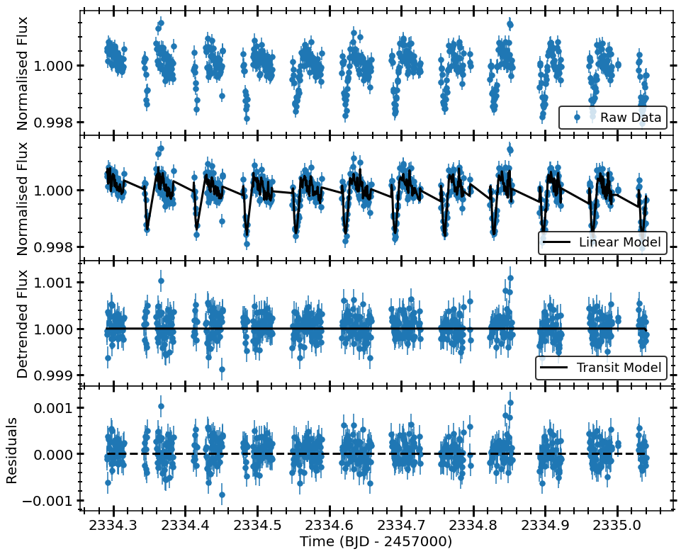
Figure 14: CHEOPS light curve of the final visit of HD 108236; (top panel) the DEFAULT DRP fluxes in blue, (second panel) the raw data in blue plus the linear model built from the PCA PSF method in black, (third panel) detrended fluxes in blue and the best fit transit model in black, and (bottom panel) the residuals to the fit in blue.

Appendix E Transit times

The results of the timing analysis of the transits as described in Sect. 5 are shown in Tables 9 and 10. These transit times are the result of the light curve fits for each planet separately, using as priors the results of the global photometric fit described in Sect. 4.

Table 9: Central time of each of the transits of planet $b$ and $c$ analyzed in this work.

Planet $b$
Epoch	T${}_{\text{c}}$	$+\sigma$	$-\sigma$	Source
0	8572.1080	0.0038	0.0032	TESS
1	8575.9000	0.0055	0.0060	TESS
2	8579.7025	0.0069	0.0082	TESS
4	8587.2939	0.0025	0.0039	TESS
5	8591.0970	0.0078	0.0043	TESS
6	8594.8917	0.0039	0.0038	TESS
7	8598.6734	0.0039	0.0028	TESS
8	8602.4686	0.0052	0.0040	TESS
9	8606.2730	0.0036	0.0050	TESS
11	8613.8544	0.0068	0.0044	TESS
12	8617.6598	0.0021	0.0021	TESS
13	8621.4498	0.0027	0.0042	TESS
102	8959.3020	0.0020	0.0019	CHEOPS
105	8970.6821	0.0028	0.0027	CHEOPS
110	8989.6601	0.0028	0.0024	CHEOPS
112	8997.2494	0.0011	0.0013	CHEOPS
113	9001.0425	0.0026	0.0052	CHEOPS
194	9308.5086	0.0044	0.0037	TESS
195	9312.3224	0.0042	0.0043	TESS
196	9316.0992	0.0052	0.0035	TESS
198	9323.6931	0.0026	0.0028	TESS
199	9327.4805	0.0040	0.0078	TESS
200	9331.2915	0.0059	0.0079	TESS
Planet $c$
Epoch	T${}_{\text{c}}$	$+\sigma$	$-\sigma$	Source
0	8572.3921	0.0015	0.0013	TESS
1	8578.5998	0.0018	0.0013	TESS
2	8584.7979	0.0038	0.0038	TESS
3	8591.0124	0.0034	0.0036	TESS
5	8603.4095	0.0025	0.0019	TESS
6	8609.6151	0.0022	0.0012	TESS
7	8615.8166	0.0041	0.0047	TESS
8	8622.0309	0.0013	0.0015	TESS
56	8919.7989	0.0013	0.0016	CHEOPS
64	8969.4285	0.0020	0.0022	CHEOPS
65	8975.6328	0.0005	0.0005	CHEOPS
66	8981.8337	0.0021	0.0019	CHEOPS
70	9006.6546	0.0008	0.0008	CHEOPS
119	9310.6308	0.0024	0.0038	TESS
120	9316.8357	0.0014	0.0013	TESS
121	9323.0385	0.0015	0.0014	TESS
122	9329.2407	0.0014	0.0013	TESS

Table 10: Central time of each of the transits of planet $d$, $e$ and $f$ analyzed in this work.

Planet $d$
Epoch	T${}_{\text{c}}$	$+\sigma$	$-\sigma$	Source
0	8571.3355	0.0016	0.0014	TESS
1	8585.5137	0.0019	0.0014	TESS
2	8599.6872	0.0015	0.0011	TESS
3	8613.8654	0.0034	0.0036	TESS
28	8968.2577	0.0011	0.0009	CHEOPS
30	8996.6104	0.0049	0.0043	CHEOPS
52	9308.4794	0.0028	0.0025	TESS
53	9322.6590	0.0022	0.0023	TESS
Planet $e$
Epoch	T${}_{\text{c}}$	$+\sigma$	$-\sigma$	Source
0	8586.5685	0.0014	0.0013	TESS
1	8606.1591	0.0012	0.0011	TESS
17	8919.5979	0.0006	0.0006	CHEOPS
21	8997.9600	0.0008	0.0008	CHEOPS
37	9311.4060	0.0011	0.0013	TESS
38	9330.9942	0.0023	0.0020	TESS
Planet $f$
Epoch	T${}_{\text{c}}$	$+\sigma$	$-\sigma$	Source
-1	8586.4885	0.0044	0.0038	TESS
0	8616.0337	0.0059	0.0050	TESS
12	8970.5272	0.0015	0.0018	CHEOPS
24	9324.9808	0.0054	0.0037	CHEOPS
24	9324.9857	0.0088	0.0087	TESS

Appendix F Radial velocities fit

The radial velocity measurements reported by Teske et al. (2021) were fitted using juliet package. The priors of the orbital parameters were defined as normal distributions using the fitted values and uncertainties of the photometric fit (Sect. 4) reported in Table 4. The full RV model as a function of time, and the phased model for each planet are shown in Figures 16 and 17, respectively. The corner plot of the posterior distributions of the fitted parameters are shown in Fig. 18.

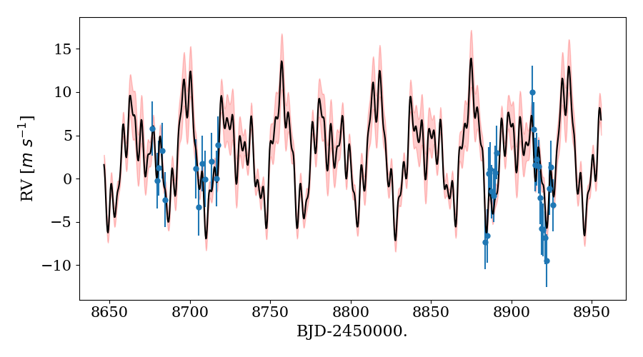
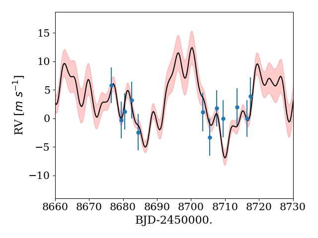
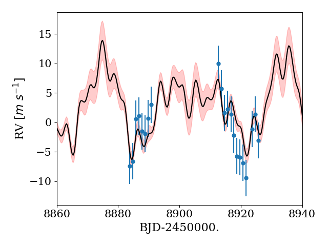
Figure 16: Radial velocity measurements from Teske et al. (2021) (blue symbols) with the best fitted model (black solid curve) and its uncertainties (red regions). The bottom panels are closer views of the top panel for the relevant time coverage of the observations. The RV error bars include the estimated jitter.

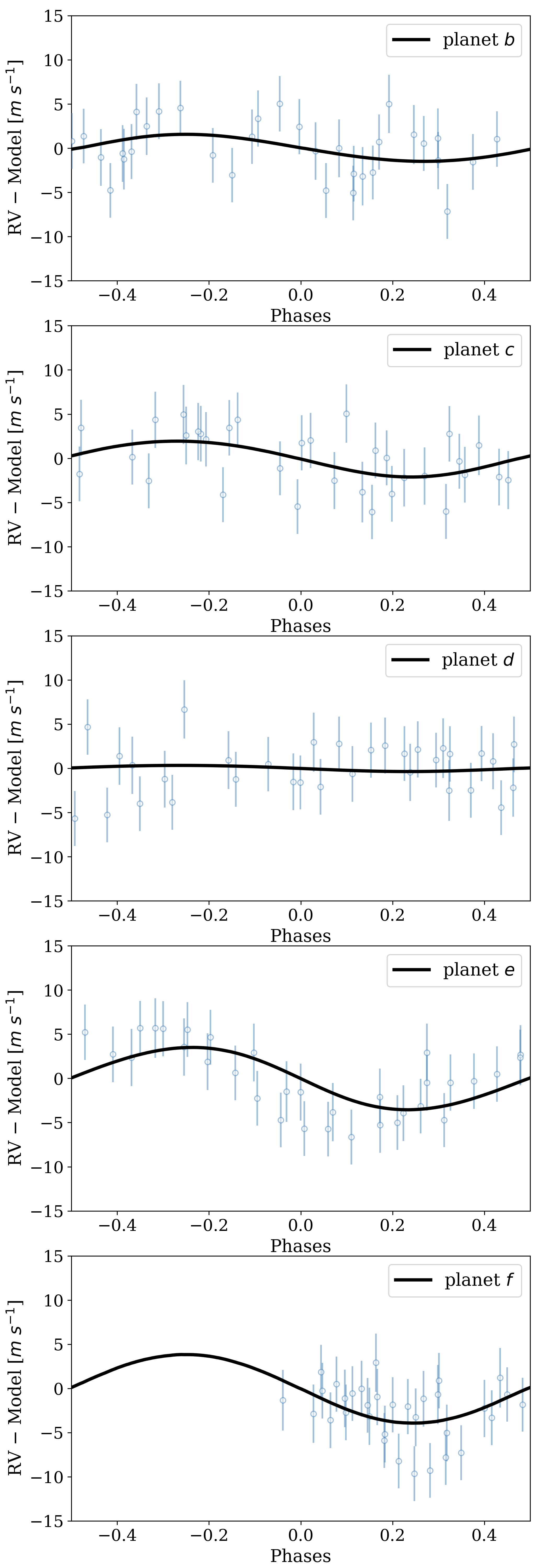
Figure 17: Phased radial velocities with the full model removed except for the component of the plotted planet (solid curve).

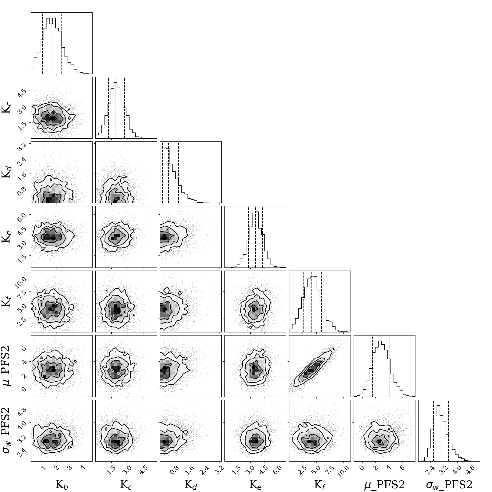
Figure 18: Corner plot of the posterior distributions of the parameters estimated by the modeling of the RV measurements of HD 108236.