Plasma composition measurements in an active region from Solar Orbiter/SPICE and Hinode/EIS

Abstract

A key goal of the Solar Orbiter mission is to connect elemental abundance measurements of the solar wind enveloping the spacecraft with EUV spectroscopic observations of their solar sources, but this is not an easy exercise. Observations from previous missions have revealed a highly complex picture of spatial and temporal variations of elemental abundances in the solar corona. We have used coordinated observations from Hinode and Solar Orbiter to attempt new abundance measurements with the SPICE (Spectral Imaging of the Coronal Environment) instrument, and benchmark them against standard analyses from EIS (EUV Imaging Spectrometer). We use observations of several solar features in AR 12781 taken from an Earth-facing view by EIS on 2020 November 10, and SPICE data obtained one week later on 2020 November 17; when the AR had rotated into the Solar Orbiter field-of-view. We identify a range of spectral lines that are useful for determining the transition region and low coronal temperature structure with SPICE, and demonstrate that SPICE measurements are able to differentiate between photospheric and coronal Mg/Ne abundances. The combination of SPICE and EIS is able to establish the atmospheric composition structure of a fan loop/outflow area at the active region edge. We also discuss the problem of resolving the degree of elemental fractionation with SPICE, which is more challenging without further constraints on the temperature structure, and comment on what that can tell us about the sources of the solar wind and solar energetic particles.

To be submitted to the Astrophysical Journal

1 Introduction

One of the most important goals of solar-terrestrial physics is to understand how the Sun generates and controls the heliosphere. There are several open questions that need to be focused on to fully address this topic. For example, what are the sources of the solar wind? Where and how are solar energetic particles (SEPs) accelerated? How does plasma propagate through the heliosphere? And how does all this information and understanding feed into a future space weather prediction capability?

With the launch of the Parker Solar Probe (PSP, Fox et al., 2016) in 2018 August, and Solar Orbiter in 2020 February (Müller et al., 2020), we now have new capabilities and instrumentation that can be brought to bear on these questions. PSP and Solar Orbiter will travel to within 0.046 and 0.26 AU, respectively, at their closest perihelia, while Solar Orbiter will also rise out of the plane of the ecliptic to observe the polar regions from up to $\sim$33^∘ heliolatitude (in the extended mission phase). Their new observations are already challenging our previous understanding of heliospheric phenomena. A new question, perhaps, is whether properties and signatures of the solar wind, or SEPs, imprinted in the solar atmosphere and measured and analyzed close to the Sun, survive propagation through the heliosphere all the way to the Earth. PSP has revealed a complex and dynamic near-Sun magnetic environment replete with field reversals, for example, see Bale et al. (2019). The ability to make measurements close-in and far-out from the Sun during the orbits of these missions will help to complete our understanding of the solar wind, SEPs, and how eruptive phenomena propagate through the heliosphere (Janvier et al., 2019).

In recent years, a great deal of work has been carried out with the Hinode spacecraft (Kosugi et al., 2007), particularly the EUV Imaging Spectrometer (EIS, Culhane et al., 2007), and several diagnostics have emerged. Techniques have been developed to utilize specific element pairs, e.g. Si/S, to trace the source regions (Brooks & Warren, 2011), and indeed, properties of spectra such as line profile asymmetries have been found to be helpful since lines of different elements sometimes show asymmetries of different magnitudes (Brooks & Yardley, 2021a). Of course elemental abundances are a key tracer for connection science, but studies of solar atmospheric composition are highly complex. The solar corona shows strong spatial and temporal variability in plasma composition (Feldman, 1992). Elements with a low FIP (first ionization potential; $<$ 10 eV) are enhanced in the corona by factors of 2–4 (FIP, Pottasch, 1963; Meyer, 1985), but differences are observed between and within long lived structures at the active region boundary and within the core, and changes from coronal composition are seen during impulsive events and flares (Baker et al., 2013; Warren, 2014; Doschek et al., 2015; Warren et al., 2016); see also the review by Del Zanna & Mason (2018). The situation in the solar wind adds further complexity, with differences in composition seen between fast and slow wind streams, substantial changes within the slow wind itself, and variability between and within different element ratios (von Steiger et al., 2000; Zurbuchen et al., 2002, 2012).

Nevertheless, the FIP effect has substantial potential for allowing us to link remote sensing spectroscopic observations with in-situ particle measurements. Despite variations, the general compositional character of active regions (ARs) is fairly well known, with closed field loops showing a FIP effect that is strongest in the core. This allows us to link atmospheric and heliospheric phenomena. For example, interplanetary coronal mass ejections (ICMEs) with elevated charge states (indicating higher temperatures) show a stronger FIP effect than is seen in the slow solar wind (Zurbuchen et al., 2016), suggesting that while the slow wind might emerge from closed field loops, these ICMEs may have been ejected from the AR core. Additionally, photospheric composition is sometimes measured in the high density cores of ICMEs with persistently low charge states (Lepri & Rivera, 2021; Rivera et al., 2022), implying that prominence material is being detected. Hinode observations have also identified previously unnoticed potential sources of the solar wind, such as outflows at the edges of active regions (Sakao et al., 2007; Del Zanna, 2008; Doschek et al., 2008; Harra et al., 2008), and these have been linked to the slow solar wind using cross-mission composition measurements between Hinode and the ACE observatory (Brooks & Warren, 2011). Although such multi-spacecraft studies have limitations, they have developed the preferred pathway for connection studies with Solar Orbiter, and built a foundation for the spectroscopic analysis from the Spectral Imaging of the Coronal Environment (SPICE, Spice Consortium et al., 2020) instrument.

SPICE itself observes a wavelength range that contains a wide range of emission lines from multiple elements, and has been designed in part to link with the Solar Wind Analyzer (SWA, Owen et al., 2020) for connection science. The combination of the Solar Orbiter instruments, together with coordinated observations from EIS and other missions, promises to advance our understanding of this key topic. Simultaneous observations with SPICE and EIS will rely on a detailed understanding of the cross-instrument calibration. Of course the first step in making progress is to understand the SPICE instrument itself, and test and benchmark the diagnostics capabilities. This is the subject of this paper. We use observations of AR 12781 on the Earth facing disk from Hinode, together with SPICE observations of the same region one week later from the short-term planning (STP-122) commissioning phase. Although the EIS and SPICE observations were not taken simultaneously, this allows us to apply well tested and standard elemental abundance measurement routines developed for EIS to understand the compositional structure of AR 12781, and apply that knowledge to the interpretation of the SPICE observations. Based on previous work with similar EIS observations of active regions we expect the strongest FIP-bias to be found at the loop footpoints (Baker et al., 2013; Brooks & Yardley, 2021b). These results suggest a link with solar energetic particles (Brooks & Yardley, 2021b), which show a higher FIP bias. Generally speaking, upflows in EIS have tended to show a coronal composition when measured using a Si/S ratio, though a photospheric composition is sometimes seen (Brooks et al., 2020). This is consistent with the slow solar wind, which shows variability from photospheric to predominantly coronal composition in Si/S measurements. Of course AR structures will evolve over a one week period, but our expectation is that the general characteristics of AR 12781 should be broadly maintained i.e. whether the bright fan loops show photospheric or coronal composition, and that similar results should be found with SPICE, using different elements, for this same active region. Furthermore, not all Solar Orbiter encounters will be on the Sun-Earth line, so there is value in exploring what can be achieved through multi-viewpoint observations, and through AR tracking on timescales longer than that taken to cross the disk. In the process of verification, we identify new methodology for determining elemental abundances and interpreting the new measurements from SPICE.

2 Data reduction

Details of the EIS and SPICE instruments are available in Culhane et al. (2007) and Spice Consortium et al. (2020). Here we describe the observations we use and some of the pertinent characteristics and data reduction methods.

The Hinode/EIS data we use were taken on 2020, November 10, at 02:08:11 UT  when the target active region (AR 12781) was close to disk center from an Earth view. EIS was constructed with an exchangeable slit-assembly that can switch between 1^′′, 2^′′, 40^′′, and 266^′′ apertures. These data were taken using the 2^′′ slit. Spectra can be obtained in two wavelength ranges from 171–211 Å  and 245–291 Å  with a spectral resolution of 23 mÅ. Generally, a subset of these ranges is telemetered to the ground, and the observing program we analyze comprised 25 wavelength windows covering a wide selection of spectral lines from ions of Mg V–Mg VII, Fe VIII–Fe XVII, Si X, S X, Ca XIV–Ca XVII, and some higher temperature Fe XXIV lines seen during flares. The observing program scans an area of 261${}^{\prime\prime}\times$512^′′ with coarse 3^′′ steps to reduce the duration to about 1 hour with an exposure time of 40 s.

The data were processed using standard procedures that are available in SolarSoft (SSW, Freeland & Handy, 1998). The routine eis_prep converts the recorded count rates to physical units (erg cm^-2 s^-1 sr^-1 Å^-1) after cleaning the data arrays of cosmic ray strikes, dusty, warm, and hot pixels, and removal of the dark current pedestal. We used the updated on-orbit photometric calibration of Warren et al. (2014) in this work. We assume an uncertainty of 23% for the line intensities (Lang et al., 2006). A known issue is that the EIS spectra drift back and forth across the CCDs (charge-coupled device) due to temperature changes and spacecraft motion around Hinode’s polar orbit. We make an initial correction for this effect using the standard neural network (ANN) model developed by Kamio et al. (2010). This method also corrects the spectral curvature and spatial offsets between the two CCDs. As discussed elsewhere (Brooks et al., 2020), this ANN model was developed using data early in the mission. As a result, a residual orbital variation in the spectra is often seen in recent data and is present in our dataset. We removed this trend using the method discussed by Brooks et al. (2020). This method involves modeling the residual variation by averaging data in the Y-direction over some portion of the field-of-view (FOV). We used the lower 50 pixels for this correction. Note that to determine the velocity calibration we use the reference wavelengths derived for the EIS spectral lines by Warren et al. (2011) using off-limb quiet Sun observations. All measurements in this paper refer to relative, not absolute, Doppler velocities.

The Solar Orbiter/SPICE data we use were taken 7 days after the EIS observations on 2020, November 17, at 22:28:26 UT. At this time, Solar Orbiter was positioned at 0.91–0.93 a.u., around 120^∘ away from Earth (counter-clockwise behind the Sun), so that AR 12781 had entered the SPICE FOV. Additional telemetry allowed for science observations to be made for several days around this time-period as part of the STP-122 commissioning phase. The SPICE instrument also operates with four slit width options: 2^′′, 4^′′, 6^′′, and 30^′′. The observations discussed here were taken using the 6^′′ slit. The spatial resolution of these SPICE observations is therefore about a factor of 2 lower than the EIS observations discussed here (using the 2^′′ slit and coarse 3^′′ steps). Spectra can be obtained in two wavelength ranges from 704–790 Å  and 973–1049 Å. The observing program we analyze recorded full detector spectra in these wavelength ranges allowing us to examine a wide selection of spectral lines from ions of O II–O VI, N III–N IV, Ne VI, Ne VIII, C III, S IV–S V, and Mg VIII–Mg IX. The SPICE observation ID for these data is 33554573 and the observing sequence is a series of single exposures scanning an area of 180${}^{\prime\prime}\times$1024^′′ in around 50 min  with an exposure time of 59.6 s at each position. The unique identifiers for the exposures we used are V06_33554573_000–V06_33554573_029 and the data were from a pre-release test. Updated versions of the same files have been released as V08/V09 by the SPICE team (Auchère, 2021). We used the SUMER spectral atlas of solar-disk features (Curdt et al., 2001) to identify the SPICE spectral lines and assign reference wavelengths that we used to derive velocities.

Several characteristics of the on-orbit performance of SPICE are still being investigated. Preliminary discussions can be found in the early results article by Fludra et al. (2021). The commissioning data were calibrated to level-2 and provided to us for individual testing prior to public release. The data reduction followed developing standard procedures that will be provided in SSW by the SPICE team. These procedures include all the calibration parameters that have been quantified to date. The units of the data are W m^-2 sr^-1 nm^-1. We assume an uncertainty of 25% for the SPICE line intensities, and this is added in quadrature to the errors from the line fits. For both SPICE, and EIS, the line intensities were obtained by fitting Gaussian functions to the spectra. Single or multiple Gaussians were used as appropriate for the specific line and any associated blends.

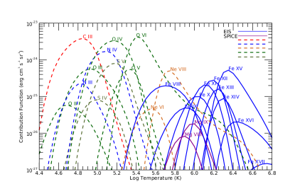
Figure 1: Contribution functions ($G(T,n)$) for many of the SPICE and EIS emission lines analyzed in this work. The plot shows the range of temperature covered by the lines. The calculations assume a constant density (n) of 10⁹ cm^-3 and the adoption of the photospheric abundances of Scott et al. (2015b) and Scott et al. (2015a). Contribution functions for the elements with FIP $>$10 eV  are shown with dashed lines. We only show the strongest line from each ionization stage for clarity. The legend indicates whether the lines are observed by EIS or SPICE. The figure shows that many of the lower temperature high-FIP lines should be relatively bright compared to the higher temperature low-FIP lines in photospheric conditions. In some regions of the corona, the low-FIP Mg and Fe lines become stronger relative to their photospheric magnitudes.

3 Atomic data and analysis methods

For an optically thin atomic transition from level $i$ to level $j$ the emission line intensity is

$$I_{i\rightarrow j}=A\int_{T}G(T,n)\phi(T)dT$$ (1)

where $A$ is the elemental abundance, $T$ is the electron temperature, $n$ is the electron density, $G(T,n)$ is the contribution function, and $\phi(T)$ is the differential emission measure (DEM). The DEM is a measure of the amount of material as a function of temperature. The form of Equation 1 assumes a relationship between temperature and density, such as constant pressure (Craig & Brown, 1976).

The contribution function, $G(T,n)$, theoretically describes the line emission through a population structure and ionization equilibrium calculation. These are computed from the relevant electron collisional excitation/deexcitation rates, spontaneous radiative decay probabilities, and ionization and recombination coefficients. For all the spectral lines studied in this work we take the electron collisional and radiative decay data from the CHIANTI database (Dere et al., 1997) version 10 (Del Zanna et al., 2021).

The $G(T,n)$ function is strongly peaked in temperature and weakly sensitive to density; primarily through the suppression of dielectronic recombination (DR) at high densities (Burgess, 1964), but also due to the effects of metastable levels, and step-wise (level stepping) ionization and auto-ionization (Summers et al., 2006). There have been occasional efforts to examine these effects in studies of the solar corona (Brooks et al., 1998; Lanzafame et al., 2002; Brooks & Warren, 2006), but often the densities are too low to show dramatic results. Conversely, the IRIS instrument observes the lower transition region and chromosphere where densities are higher, so there has been a renewed interest in including this effect (Young et al., 2018). SPICE observations span an intermediate temperature and density regime where improved spectroscopic accuracy may also be important (Parenti et al., 2019). Here we adopt the density dependent ionization equilibrium calculations from the generalized collisional-radiative models of ADAS (Summers et al., 2006) for the elements C, N, O, Ne, and Si, and supplement them with calculations for Mg, S, and Fe using the CHIANTI approximate DR suppression models of Nikolić et al. (2018).

Our plasma composition measurement technique for EIS is now fairly well established (Brooks & Warren, 2011). We select a series of spectral lines from Fe VIII–Fe XVII for the DEM analysis (Equation 1). We then use the Fe XIII 202.044/203.826 diagnostic ratio to compute the electron density, and calculate the $G(T,n)$ function for all the spectral lines adopting the photospheric elemental abundances of Scott et al. (2015b) and Scott et al. (2015a). The DEM is computed at this constant density using the Markov-Chain Monte Carlo (MCMC) algorithm included in the PintOfAle software package (Kashyap & Drake, 1998, 2000). The MCMC algorithm constructs the DEM by performing 100 simulations that minimize the differences between the observed and computed line intensities and converge to a best-fit solution. Once the DEM is established from the low-FIP Fe lines, we use it as the basis for computing the FIP bias from the Si X 258.375 Å  to S X 264.223 Å  ratio. Since Si is a low-FIP element, the 258.375 Å  intensity should be well represented by the Fe-only DEM. We check, however, that there is no large systematic difference, and adjust the DEM to match the Si X 258.375 Å  intensity. We then use the adjusted DEM to predict the S X 264.223 Å  intensity. The ratio of the DEM-calculated intensity to the observed intensity gives us the FIP bias because the S X 264.223 Å  intensity predicted by the DEM from the low-FIP elements will be too large/correct depending on whether the actual abundances are coronal/photospheric. S lies on the boundary between low- and high-FIP elements and shows variable behavior that is sometimes consistent with one group or the other. In some theoretical models this depends on the open or closed topology of the magnetic field (Laming et al., 2019; Kuroda & Laming, 2020), making it a useful diagnostic regardless (Brooks & Yardley, 2021b).

For SPICE, our purpose is to develop a new useful technique and benchmark it against the EIS results. This task is challenging for two reasons. First, the SPICE temperature coverage does not extend far beyond 1 MK  in non-flaring coronal conditions. This can be seen from a plot of the $G(T,n)$ functions for the lines investigated in this work in Figure 1. The figure also shows the $G(T,n)$ functions for the EIS lines for comparison. The highest temperature SPICE lines from Mg IX reach about 1 MK, and these are also the boundary constraints for the DEM analysis which makes matters more difficult; though higher temperature lines may be detectable in second order in other datasets with longer exposures, or in flares (Spice Consortium et al., 2020). Some studies of full-disk observations of the Sun suggest that the FIP effect is only detectable above 1 MK  (Laming et al., 1995), which puts the highest temperature SPICE lines at the limit of where the effect would be detectable. This could be problematic for studies of spectra averaged over large spatial scales and deserves our attention. Of course most SPICE observations will concentrate on specific features. Several previous analyses have shown that spikey structures at the edges of active regions - more recently named fan loops - can show a strong FIP effect in the upper transition region when measured using Mg/Ne ratios (Sheeley, 1996; Young & Mason, 1997; Widing & Feldman, 2001) or Fe/O (Warren et al., 2016). These results are relevant to our analysis in section 4. Furthermore, there are some indications from full-disk SDO/EVE spectra that the FIP effect can be detected at somewhat lower temperatures (0.5 MK, Brooks et al., 2017). Secondly, the best spectral lines from low- and high-FIP elements at the high temperature end of the SPICE capabilities come from Mg VIII–Mg IX and Ne VIII. These ions do not have a good overlap in temperature, and Ne VIII is a Li-like ion so has a large high temperature tail that can influence the measured FIP bias if it is not modeled correctly. There are two Ne VIII lines and five Mg VIII–Mg IX lines, however, which should provide good constraints, and additional lines from lower temperature ions of S IV and S V. It may also be possible to develop a measurement technique from linear combinations of spectral lines; such as has been developed for EIS by Zambrana Prado & Buchlin (2019). Parenti et al. (2021) have also discussed using composition data to link spacecraft measurements in the solar wind to their sources, and specifically compare results from the Zambrana Prado & Buchlin (2019) method to a DEM technique that is comparable to what we have used here.

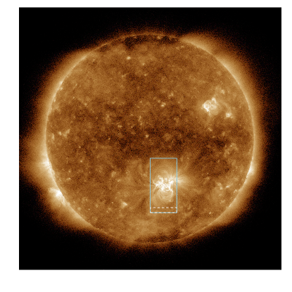
Figure 2: SDO/AIA 193 Å  image of the solar corona showing AR 12781 on 2020, November 10, at 02:38:04 UT. The sky blue box shows the field-of-view (FOV) of the EIS slit scan from 02:08:11–03:08:16 UT. The white dashed box shows the area used for velocity calibration (see text).

For SPICE, we do not have sufficient temperature coverage from spectral lines of one species to perform the EM analysis for a single element. We also do not have sufficient coverage to do the analysis for low-FIP elements only. We therefore follow a different approach. We identify a sample of spectral lines from O II–O VI, S IV–S V, N III–N IV, C III, Ne VI, Ne VIII, and Mg VIII–Mg IX using the SUMER spectral atlas of on-disk features (Curdt et al., 2001). We then compute the electron density using the Mg VIII 772.31/782.34 diagnostic ratio, and calculate the $G(T,n)$ function for all the spectral lines. The DEM is computed at this constant density again using the MCMC algorithm and assuming a fixed set of elemental abundances. We then look for consistency between the observed and calculated intensities to determine which set of abundances best represents the observations.

Since most of the spectral lines we use ($\sim$ 80%) are from high FIP elements, there is a possibility that changing the abundances for these elements could lead to better DEM convergence simply because they dominate the sample. This would make it appear that a FIP effect has been detected, when in fact it is only a result of adopting a different set of abundances. To avoid any confusion as to the reasons why a particular abundance set provides a better solution, in the case of SPICE, we adopt photospheric abundances for the high-FIP elements even in the corona. More precisely, only the low-FIP elements are enhanced in our coronal abundance dataset (by the factor recommended by Schmelz et al., 2012).

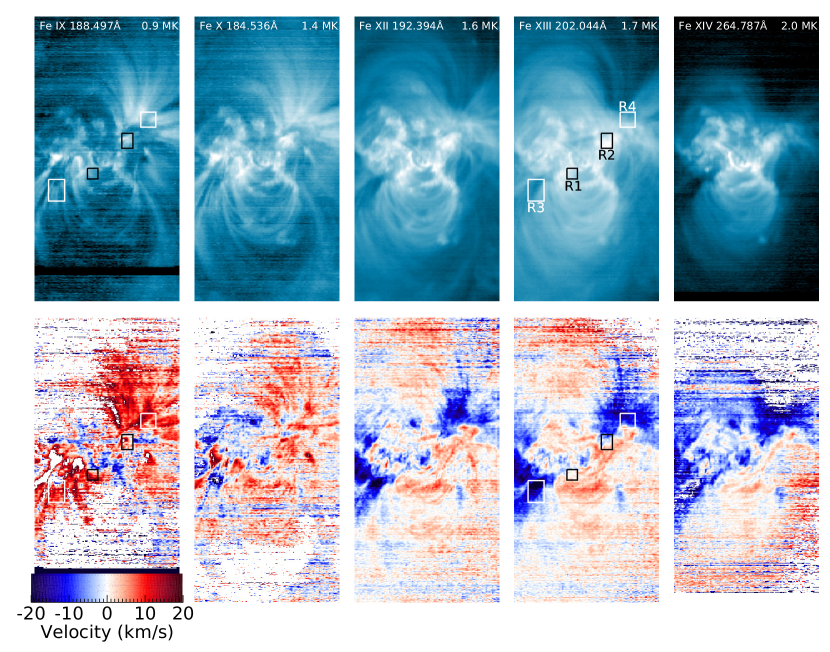
Figure 3: Intensity and velocity maps of AR 12781 constructed from the EIS scan from 02:08:11–03:08:16 UT. Upper row: Intensity maps covering a range of temperatures from 0.9–2.0 MK using spectral lines of Fe IX–Fe XIV. Lower row: Velocity maps obtained from single Gaussian fits to the corresponding spectral lines. Red/blue show plasma moving away/towards the observer. The white/black boxes labeled R1–R4 highlight the areas in the active region upflows/loop footpoints selected for the elemental abundance analysis.

4 Results and discussion

AR 12781 appeared on the solar east limb on 2020, November 3. It was a bipolar region and produced numerous C-class flares during its Earth-facing disk passage. According to the Hinode Flare Catalog (Watanabe et al., 2012), however, all but one of these flares (26/27), occurred prior to the EIS observations on November 10, so any impact on the compositional structure of AR 12781 between the EIS and SPICE observations is likely to be minimal. Figure 2 shows the AR on a full disk AIA 193 Å  image, with the EIS slit scan FOV overlaid. Figure 3 shows examples of the EIS observations for a range of temperatures. Bright fan loops can be seen to the east and west sides at lower temperatures ($\sim$0.9–1.4 MK), with high lying loops in the central structure ranging to higher temperatures ($\sim$0.9–2.0 MK). Bright moss emission can be seen in the AR core. The cooler fan loops are red-shifted, while characteristic blue-shifted upflows are seen at the AR edges; mixing with the fans. These features are typical of EIS observations of large bipolar regions (Del Zanna, 2008; Brooks & Warren, 2011; Warren et al., 2011).

We selected four regions in the AR for our composition analysis. R1 is a bright moss region at the base of high temperature loops and R2 is at the footpoint of a fan loop at the AR edge, while R3 and R4 were chosen to sit in the upflows that are seen as blue-shifted in the Fe XIII 202.044 Å  velocity map of Figure 3. R2 and R4 are within the area that is later observed by SPICE.

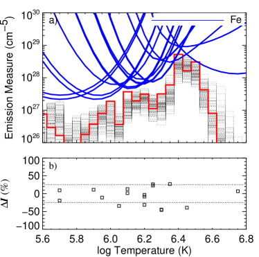
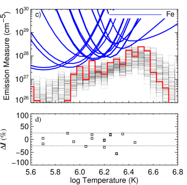
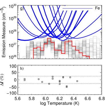
Figure 4: EIS emission measure (EM) analysis of the regions selected on 2020, November 10. The upper panels in each quadrant show the EM analysis. The red line shows the best-fit solution to a series of Monte Carlo simulations (shown as dotted grey lines). The blue lines are emission measure loci curves for each of the spectral lines used in the analysis. These visualize the upper limits to the emission measure for each line of each ion. The element for each line is also identified in the legend. The lower panels in each quadrant show the differences between the measured and calculated intensities. They are given as percentages of the observed intensities. The dotted lines indicate departures of 25%. We show the results for region R1 in panels a & b; R2 in panels c & d; R3 in panels e & f; and R4 in panels g & h.

We show our emission measure (EM) analysis of the four regions in Figure 4, together with a comparison of the observed and EM calculated intensities. We also provide the observed and calculated intensities, and the percentage differences between them, for all four regions in Table 1. In most cases (80–90%) the differences between the observed and calculated intensities are less than $\sim$35%; indicating that the best-fit MCMC solution is reproducing the observed intensities well. The Fe XIV line pair (270.519 Å  and 264.787 Å) seem to be consistently stronger than predicted in all four regions. This is clear from the EM plots in Figure 4: the Fe XIV loci curves that minimize at $\log$ T = 6.3, with T in units of K, sit above the loci curves for the adjacent ions. The reasons for this discrepancy are unclear.

Table 1: EIS DEM analysis on 10-Nov-2020

	R1			R2			R3			R4
ID	Iobs	Icalc	$\Delta[\%]$	Iobs	Icalc	$\Delta[\%]$	Iobs	Icalc	$\Delta[\%]$	Iobs	Icalc	$\Delta[\%]$
Fe VIII 185.213	574.8$\pm$126.5	463.3	-19.4	630.9$\pm$138.8	521.7	-17.3	244.7$\pm$53.9	233.2	-4.7	486.6$\pm$107.1	476.9	-2.0
Fe VIII 186.601	297.9$\pm$65.6	325.2	9.2	350.0$\pm$77.0	365.3	4.4	160.1$\pm$35.2	166.0	3.7	318.4$\pm$70.1	337.7	6.1
Fe IX 188.497	108.3$\pm$23.9	120.1	10.9	159.9$\pm$35.2	198.0	23.8	67.5$\pm$14.9	70.3	4.1	179.9$\pm$39.6	188.0	4.5
Fe IX 197.862	61.9$\pm$13.6	55.2	-10.9	104.9$\pm$23.1	95.6	-8.8	39.9$\pm$8.8	36.5	-8.6	112.2$\pm$24.7	96.5	-14.0
Fe X 184.536	616.0$\pm$135.6	405.3	-34.2	954.1$\pm$209.9	693.8	-27.3	309.9$\pm$68.2	231.8	-25.2	760.6$\pm$167.4	558.8	-26.5
Fe XI 188.216	937.5$\pm$206.3	1058.9	13.0	1410.1$\pm$310.2	1671.5	18.5	387.7$\pm$85.3	458.3	18.2	832.4$\pm$183.1	1013.5	21.8
Fe XI 188.299	624.0$\pm$137.3	633.4	1.5	967.8$\pm$212.9	1004.4	3.8	255.0$\pm$56.1	279.2	9.5	570.9$\pm$125.6	617.2	8.1
Fe XII 195.119	1831.5$\pm$402.9	1680.3	-8.3	2505.4$\pm$551.2	2401.0	-4.2	599.3$\pm$131.8	509.5	-15.0	1076.8$\pm$236.9	943.9	-12.3
Fe XII 192.394	558.0$\pm$122.8	540.0	-3.2	789.3$\pm$173.7	770.9	-2.3	166.1$\pm$36.5	163.3	-1.6	322.7$\pm$71.0	302.5	-6.2
Fe XIII 202.044	946.7$\pm$208.3	1198.5	26.6	1263.9$\pm$278.1	1509.3	19.4	307.1$\pm$67.6	371.4	20.9	513.0$\pm$112.9	607.7	18.5
Fe XII 203.720	211.7$\pm$46.7	145.4	-31.3	283.0$\pm$62.4	197.0	-30.4	45.0$\pm$10.0	33.0	-26.5	86.3$\pm$19.1	62.2	-27.9
Fe XIII 203.826	1303.6$\pm$286.9	1598.6	22.6	1422.2$\pm$313.0	1669.2	17.4	152.8$\pm$33.7	182.4	19.4	260.8$\pm$57.5	305.6	17.2
Fe XIV 270.519	1728.5$\pm$380.3	955.5	-44.7	1719.6$\pm$378.3	753.0	-56.2	172.4$\pm$37.9	107.1	-37.9	296.0$\pm$65.1	167.8	-43.3
Fe XIV 264.787	3222.6$\pm$709.0	1745.7	-45.8	2964.1$\pm$652.1	1327.6	-55.2	279.7$\pm$61.5	170.3	-39.1	515.7$\pm$113.5	267.3	-48.2
Fe XV 284.160	15727.2$\pm$3460.0	19960.7	26.9	10778.2$\pm$2371.2	13035.2	20.9	1187.6$\pm$261.3	1475.2	24.2	1675.9$\pm$368.7	1968.1	17.4
Fe XVI 262.984	1860.5$\pm$409.3	1128.0	-39.4	898.7$\pm$197.7	791.8	-11.9	62.9$\pm$13.8	64.0	1.7	68.9$\pm$15.2	63.0	-8.5
Fe XVII 254.87	19.7$\pm$4.4	21.1	6.8

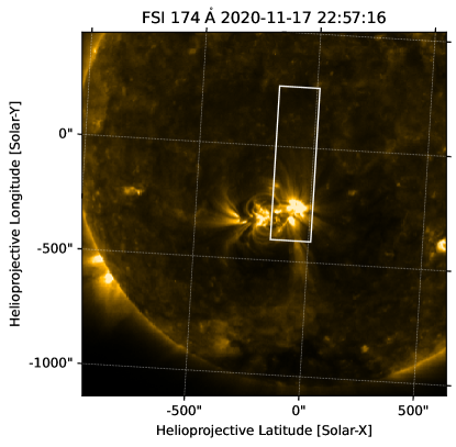
Figure 5: Solar Orbiter EUI/FSI 174 Å  image of the solar corona showing AR 12781 on 2020, November 17, at 22:57:16 UT. The white box shows the FOV of the SPICE slit scan from 22:28:26–23:19:40 UT.

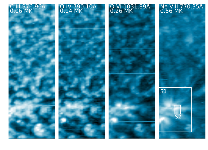
Figure 6: Intensity maps of AR 12781 constructed from the SPICE scan from 22:28:26–23:19:40 UT. The panels show intensity maps covering a range of temperatures from 0.06–0.56 MK using spectral lines of C III, O IV, O VI, and Ne VIII. The white boxes labeled S1 and S2 highlight the areas in the active region/loop footpoint selected for the elemental abundance analysis.

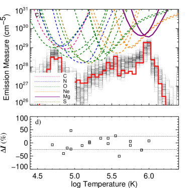
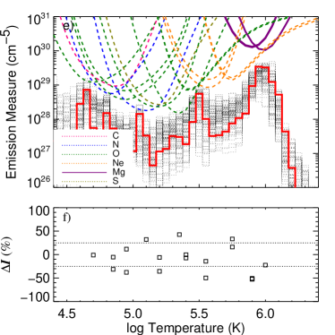
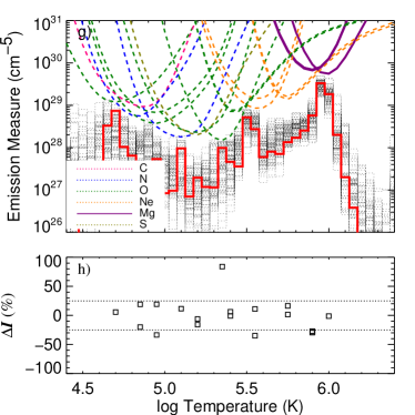
Figure 7: SPICE emission measure analysis of the regions selected on 2020, November 17. The upper panels in each quadrant show the EM analysis. The red line shows the best-fit solution to a series of Monte Carlo simulations (shown as dotted grey lines). The colored lines are emission measure loci curves for each of the spectral lines used in the analysis. These visualize the upper limits to the emission measure. The element for each line is identified by color in the legend. The solid loci curves indicate lines from low-FIP elements and the dashed loci curves indicate lines from high-FIP elements. The lower panels in each quadrant show the differences between the measured and calculated intensities. They are given as percentages of the observed intensities. The dotted lines indicate departures of 25%. We show the photospheric results for region S1 in panels a & b; the coronal results for S1 in panels c & d; the photospheric results for S2 in panels e & f; and the coronal results for S2 in panels g & h.

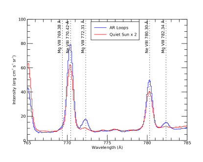
Figure 8: Comparison of loop footpoint (blue; region S2) and quiet Sun (red) SPICE spectra for the 765–785 Å  wavelength range where critical low FIP Mg VIII and high FIP Ne VIII spectral lines fall. We scaled the quiet Sun spectrum by a factor of 2 in order to show the relative strengths of the Mg VIII lines. They are stronger when the low FIP elements are enhanced in the corona. The line identifications are given in the vertical legends.

Table 2: SPICE DEM analysis on 17-Nov-2020

		S1 - Photospheric		S1 - Coronal			S2 - Photospheric		S2 - Coronal
ID	Iobs	Icalc	$\Delta[\%]$	Icalc	$\Delta[\%]$	Iobs	Icalc	$\Delta[\%]$	Icalc	$\Delta[\%]$
O III 702.61	20.2$\pm$6.1	15.4	-23.6	15.4	-23.6	22.3$\pm$6.6	13.9	-37.8	14.8	-33.6
O III 703.87	19.2$\pm$5.7	28.2	46.6	28.2	46.6	22.7$\pm$6.5	25.3	11.7	27.0	19.1
Mg IX 706.02	12.5$\pm$3.5	7.7	-37.9	13.4	7.5	19.1$\pm$5.1	14.8	-22.5	18.8	-1.2
O II 718.49	7.2$\pm$2.2	7.5	5.0	6.6	-7.2	7.8$\pm$2.4	7.8	-1.0	8.3	5.7
O V 760.43	11.2$\pm$5.0	11.6	3.3	13.2	17.7	2.2$\pm$1.9	3.1	42.6	4.0	83.9
N IV 765.15	30.1$\pm$8.0	24.7	-18.1	27.0	-10.3	32.8$\pm$8.6	43.4	32.2	36.6	11.5
Mg VIII 769.38						2.2$\pm$1.9	1.1	-50.8	1.6	-27.1
Ne VIII 770.42	42.8$\pm$11.2	46.8	9.1	45.3	5.8	67.2$\pm$17.2	89.5	33.3	78.2	16.4
Mg VIII 772.31	5.7$\pm$2.4	2.1	-63.6	4.2	-27.3	10.4$\pm$3.3	4.9	-52.2	7.3	-29.3
Ne VIII 780.30	24.7$\pm$6.6	23.1	-6.3	22.4	-9.2	38.1$\pm$9.9	44.3	16.3	38.7	1.5
Mg VIII 782.34	4.5$\pm$2.4	1.6	-63.7	3.2	-27.4	6.8$\pm$2.7	3.2	-52.3	4.8	-29.5
S V 786.47	16.2$\pm$4.8	12.9	-20.5	16.2	0.0	21.7$\pm$6.2	14.0	-35.6	18.2	-16.0
O IV 787.72	30.5$\pm$8.3	30.7	0.7	31.7	4.1	38.6$\pm$10.3	36.3	-6.0	36.3	-6.1
C III 977.03	415.2$\pm$104.0	354.3	-14.7	334.1	-19.5	430.7$\pm$107.9	295.2	-31.5	344.2	-20.1
N III 991.55	25.8$\pm$7.3	16.1	-37.3	15.3	-40.4	12.3$\pm$4.8	11.6	-5.4	14.6	19.1
Ne VI 999.27	5.9$\pm$2.2	2.4	-59.8	2.9	-50.8	6.6$\pm$2.3	3.3	-49.8	4.3	-34.9
Ne VI 1005.79	1.4$\pm$1.2	1.4	3.6	1.8	26.8	2.3$\pm$1.4	1.9	-14.3	2.5	11.0
O VI 1031.93	175.6$\pm$44.7	194.8	10.9	206.6	17.7	273.7$\pm$69.0	272.6	-0.4	290.9	6.3
O VI 1037.64	105.7$\pm$27.9	96.8	-8.4	102.7	-2.9	145.9$\pm$38.5	135.5	-7.1	144.5	-0.9

The loop footpoint regions (R1 and R2) show EM distributions that are quite strongly peaked around 2.5–3.2 MK. This is quite typical of the EM distributions found in AR cores (Warren et al., 2012), albeit a slightly lower temperature. The densities in these regions were measured at $\log$ n = 9.1 and 9.0, with n in units of cm^-3, and the FIP bias measured using the Si/S ratio is 3.1 and 2.5 in R1 and R2, respectively. The EM distributions for the upflow regions (R3 and R4) are somewhat flatter. Based on the velocity maps in Figure 3 it is likely that the emission from lines below 1 MK  do not come from the upflows. The fan loops are red-shifted and there is contamination from foreground and background emission that complicates the interpretation. Furthermore, the high temperature Fe XVII lines are too weak to measure in these quieter regions (also in R2). Nevertheless the density in both these regions is $\log$ n = 8.6, and the FIP bias measured using the Si/S ratio is 1.6 and 1.2 in R3 and R4, respectively.

The FIP related enhancement in upflow region R3 is relatively weak, though probably above the uncertainty level so that it is likely real. In region R4 the FIP bias is consistent with photospheric abundances, or the fractionation of S. Similarly variable results have been found for the upflows before (Brooks et al., 2020).

AR 12781 rotated out of the Earth-facing view and arrived in the SPICE FOV on 2020 November 17. Figure 5 shows the AR on an Extreme Ultraviolet Imager (EUI, Rochus et al., 2020) Full Sun Imager (FSI) 174 Å  image, with the SPICE slit scan FOV overlaid. Figure 6 shows examples of the SPICE observations for a range of temperatures below those accessed by EIS observations. The bright chromospheric network can be seen at 0.06–0.26 MK. It appears that the SPICE FOV mainly captures the western fan loop region observed by EIS and shown in Figure 3. The Ne VIII 770.35 Å  intensity image shows the bright moss emission at the base of the fan loops. Currently, there is an ongoing effort to understand the impact of systematic biases in SPICE Doppler velocity measurements linked to peculiarities of the telescope and spectrometer; based on the EIS Fe IX 188.497 Å  velocity map, however, these structures are likely to be red-shifted.

The Ne VIII 770.35 Å  line is formed around 0.56 MK. Unfortunately, this temperature is too low to see the upflows, which are usually seen above $\sim$1 MK in EIS observations, and construction of SPICE velocity maps at these higher temperatures (e.g. using Mg IX) is difficult. We focused on two regions in the SPICE FOV. S1 encompasses most of the bright fan region and was chosen to make sure a strong signal was obtained. S2 is at the base of the fan loops and was chosen for comparison with the EIS observations. The fan loops on the western side of the AR do not appear markedly different from when they were observed by EIS, and region S2 is approximately the same area as R4. We were not able to obtain reliable results for region R2.

We show our EM analysis of the two regions in Figure 7, together with a comparison of the observed and EM calculated intensities. We also provide the observed and calculated intensities, and the percentage differences between them, for both regions in Table 2. Note that we provide the SPICE intensities in the original SI units but that we convert them to cgs units for consistency with the EIS intensities when calculating the EM. Also, although we identified and attempted to fit about 26 lines in the SPICE spectra, several lines were either too weak to be useful or had errors larger than the measured intensities. We removed these from our EM analysis. Several lines from O IV and O V were excluded in this way, but more importantly, several high-FIP element lines were also affected. S IV 748.40 Å  and S IV 750.20 Å  may be useful in other studies of elemental abundances in the lower transition region, but are not critical for comparisons with EIS coronal measurements. The Mg IX 749.54 Å  line, however, could have been useful for our analysis but was very weak in our spectra. Mg VIII 769.38 Å  was also affected in region S1 (see Table 2).

As discussed, we do not have a good abundance diagnostic ratio from two lines formed in the same temperature range, so here we assess how well the line intensities are reproduced depending on whether we adopt photospheric or coronal abundances for the EM analysis (with special emphasis on the Mg VIII lines). Figure 7 and Table 2 show the results for both these calculations for both regions.

The purpose of the MCMC algorithm is to minimize the differences between the observed and calculated intensities, so it is no surprise that a reasonable solution is obtained for all the examples. When adopting photospheric abundances, $\sim$65% of the line intensities are reproduced to within $\sim$35% for both regions S1 and S2. There is a clear improvement, however, when using coronal abundances: 85–95% of the line intensities are reproduced. There is some scatter in the behavior for the lines from high-FIP elements: some of them are better reproduced, while others become worse. For plasma composition studies, the behavior of the lines from high-FIP elements is the main interest. The only S line in the analysis is S V 786.47 Å. It is reproduced in both regions with photospheric abundances, but the agreement is improved with coronal abundances. For this analysis, S is treated as a high-FIP element so the assumed abundance is the same in both datasets. As we discussed in section 3, S often shows unusual behavior and can act like a low-FIP element. Note, however, that if we enhance the S abundance by the factor given by Schmelz et al. (2012) then the agreement between calculated and observed intensity worsens. This suggests that treating S as a high-FIP element is valid for this dataset. However, the critical point is that the Mg VIII lines show a clear difference. Mg VIII 772.31 Å, and Mg VIII 782.34 Å  are too weak by factors of 2.1–2.8 for both regions S1 and S2 when photospheric abundances are used, and Mg VIII 769.38 Å  is also too weak by a factor of 2 in region S2. In contrast, all three lines are reproduced when coronal abundances are assumed. This can also be seen in the EM plots, where the Mg VIII EM loci curves sit above the general trend when photospheric abundances are used (panels a and e), but are more consistent with the other curves when coronal abundances are assumed (panels c and g). We show example spectra to illustrate the behavior of the Mg VIII lines compared to the Ne VIII lines in Figure 8. We clearly see that the Mg VIII lines are strong in footpoint region S2 relative to a quiet Sun control spectrum (dashed box region in Figure 5). Significantly, the calculated intensities for all the Mg VIII and Mg IX lines in S1, and the Mg VIII 772.31 Å, and Mg VIII 782.34 Å  lines in S2, are outside the error bars on the measured intensities when photospheric abundances are assumed. None of the calculated intensities for these lines are outside the error bars when coronal abundances are adopted. Effectively there is no temperature structure that can explain the Mg and Ne intensities simultaneously with photospheric abundances.

The EM distributions themselves show expected characteristics: the magnitude of the EM is higher in the transition region and low corona than measured by EIS, and the curves fall to a minimum in the $\log$ T = 5.0–5.3 range. There is some complex structure in the EM distributions that can be understood as arising from the MCMC algorithm reducing the differences between the observed and calculated intensities before the curves then rise with increasing temperature until the upper boundary defined by the Mg IX lines is reached. Recall that in section 3 we discussed how the EM is constrained at high temperatures by the low-FIP Mg IX lines. If even higher temperature lines were observed, the Mg IX lines would add to the low-FIP diagnostic capability, but in practise their usefulness depends on how the MCMC solution adapts to attempt to reproduce these lines with different assumed abundances since they set the higher boundary limit of the EM distribution. In S1 the Mg IX 706.02 Å  line intensity is reproduced only with coronal abundances, whereas in S2 it is reproduced with both photospheric and coronal abundances.

It is difficult with this technique to put a number on the FIP bias. We can say that the Mg enhancement factor in the adopted elemental abundance data is a factor of 1.9, and this works. We can see in Table 2, however, that the Mg VIII lines would be reproduced better if the Mg abundance were increased by a factor of 1.4. This implies a FIP bias of 2.7; a number that is also closer to the EIS results for the loop footpoint regions. At first sight the results for approximately the same region (EIS R4 and SPICE S2) appear inconsistent, but are in fact in line with what we would expect based on our understanding of the plasma compositional structure of active regions. At the temperatures of the SPICE measurements, we are detecting a strong FIP effect in the red-shifted fan loops. At the higher temperatures accessed by EIS, we are measuring the composition of the upflows and these show a range of values. Note also that the measurements are made with different element pairs, and of course since the observations were taken one week apart we should also consider the evolution of plasma composition in decaying ARs. Nevertheless, the combination of SPICE and EIS shows potential for allowing us to disentangle the compositional structure of active regions at different temperatures.

An alternative is to derive the FIP bias from a minimization of the chi squared value for the Mg VIII lines. This results in a similar range of values (2.6–2.7). Our analysis demonstrates that determining whether a solar feature has a photospheric or coronal composition is possible with SPICE observations. Making a more accurate measurement of the FIP bias is more challenging. This can also be achieved with simple techniques like the chi squared minimization we mention here, but of course results in uncertainties (40% in our case). The EIS observations show that the FIP bias in the upflow regions is smaller than at the loop footpoints. This is in line with our expectations developed from studies of the upflows/loop footpoints as potential slow wind/SEP sources. The difference for AR 12781 is around a factor of 2, which is potentially large enough to be detectable by SPICE with the methods we have employed. This is encouraging for SPICE connection studies going forward.

There is some evidence of fractionation between Si and Fe in our EIS measurements. For the upflow regions, the scaling factor we needed to apply to the Fe-only EM to reproduce the Si X 258.375 Å  line is around the 30–40% level. This is close to the EIS calibration uncertainty for an intensity ratio. For the loop footpoints, however, the scaling was significantly larger (a factor of 1.8–1.9). It is tempting to suggest that Si and Fe are fractionating in the closed magnetic field of the loop footpoints, but not on the open field of the upflows. In the ponderomotive force model of the FIP effect the Fe/Si ratio is close to 1.0 for the full range of slow-mode wave amplitudes on open magnetic field (Table 4, Laming, 2015). In contrast, the Fe/Si ratio reaches 1.9 at the high end of wave amplitudes on closed field (Table3, Laming, 2015). Of course we cannot rule out the possibility of cross-detector calibration uncertainties. Most of the Fe lines used for the EM analysis fall on the short-wavelength (SW) detector whereas the critical Si line falls on the long-wavelength (LW) detector. We have already noted a discrepancy for the Fe XIV lines on the LW detector.

5 Conclusion

In this initial study, we combined Hinode/EIS observations of AR 12781 taken from an Earth facing view, with Solar Orbiter/SPICE measurements obtained one week later from a longitude of 120^∘ West compared to Earth. The aim was to develop a plasma composition measurement technique for use with SPICE, and benchmark it against results from a well tested DEM method routinely used to obtain the Si/S abundance ratio with EIS.

Using the EIS measurements, we characterize the general compositional structure of the AR, to ensure that it is a typical region. As expected from previous work, the strongest FIP effect is seen in the loops in the core of the AR, especially at the footpoints. Outflows on the eastern side also show a coronal composition, but on the western side they show a photospheric composition, which is relatively rare.

Lacking a robust abundance diagnostic ratio with a good temperature overlap between lines from high- and low-FIP elements for SPICE, we looked solely for consistency between observed and DEM predicted intensities under the assumption of photospheric or coronal abundances. Measurements of the bright fan structures on the western side are consistent with a coronal Mg/Ne composition, and again, the results suggest a stronger FIP effect at the loop footpoints. These results demonstrate that SPICE can be used to detect coronal Mg/Ne abundances.

Based on previous work (Warren et al., 2011), the fan loops are expected to show red-shifts at the temperatures accessed by SPICE ($\sim$ 0.56 MK), and those structures are embedded below the blue-shifted outflows EIS observed previously at higher temperatures ($\sim$ 0.9 MK). The fan loops have a coronal Mg/Ne composition, consistent with earlier work, with the outflows above showing a photospheric composition. Although these observations were not taken simultaneously, this mixed, variable composition from an AR edge that shows outflows has been identified previously as a feature that could explain the variability in composition observed in the solar wind (Brooks et al., 2020). This analysis demonstrates the power of EIS and SPICE to work in combination to disentangle the observed emission contributions from different structures with different elemental abundances in an area of AR outflows; a capability with potential for use in other situations, discussed in the introduction, such as the detection of the mixed composition in the core of ICMEs and coronal abundances in the surrounding plasma.

Our study has been based on establishing the general compositional structure of an AR with EIS and inferring consistency in subsequent observations with SPICE. Moving forward we aim to use both simultaneous measurements and complementary multi-viewpoint observations to understand the mean magnitude and degree of variability of coronal/photospheric abundance ratios for different element pairs at diferent temperatures, so that more exact comparisons with the in situ solar wind data can be made. The small-scale spatial distribution of abundances in active regions also needs to be established definitively, though some advances in this direction have been made by Mihailescu et al. (2022). Such studies will allow both broader comparisons with composition variability in the solar wind, and direct matching between measurements with Solar Orbiter/SWA and abundance ratios in source regions identified by magnetic connectivity models.

Finally, our observations were taken during the Solar Orbiter commissioning window, when an AR fortunately passed into the FOV. The mission is now in the nominal phase, and dedicated active region SOOPs (Solar Orbiter Observation Plans) will be made on a regular basis that will provide a continuing understanding of the SPICE capabilities, in addition to solar wind and SEP connection science.

References

- Auchère (2021) Auchère, F. 2021, Data issued from SPICE instrument on Solar Orbiter : 1st data release, IDOC, doi:10.48326/IDOC.MEDOC.SPICE.1.0
- Baker et al. (2013) Baker, D., Brooks, D. H., Démoulin, P., et al. 2013, ApJ, 778, 69
- Bale et al. (2019) Bale, S. D., Badman, S. T., Bonnell, J. W., et al. 2019, Nature, 576, 237
- Brooks et al. (2017) Brooks, D. H., Baker, D., van Driel-Gesztelyi, L., & Warren, H. P. 2017, Nature Communications, 8, 183
- Brooks et al. (1998) Brooks, D. H., Summers, H. P., Harrison, R. A., Lang, J., & Lanzafame, A. C. 1998, Ap&SS, 261, 91
- Brooks & Warren (2006) Brooks, D. H., & Warren, H. P. 2006, ApJS, 164, 202
- Brooks & Warren (2011) —. 2011, ApJ, 727, L13
- Brooks & Yardley (2021a) Brooks, D. H., & Yardley, S. L. 2021a, MNRAS, 508, 1831
- Brooks & Yardley (2021b) —. 2021b, Science Advances, 7, eabf0068
- Brooks et al. (2020) Brooks, D. H., Winebarger, A. R., Savage, S., et al. 2020, ApJ, 894, 144
- Burgess (1964) Burgess, A. 1964, ApJ, 139, 776
- Craig & Brown (1976) Craig, I. J. D., & Brown, J. C. 1976, A&A, 49, 239
- Culhane et al. (2007) Culhane, J. L., Harra, L. K., James, A. M., et al. 2007, Sol. Phys., 243, 19
- Curdt et al. (2001) Curdt, W., Brekke, P., Feldman, U., et al. 2001, A&A, 375, 591
- Del Zanna (2008) Del Zanna, G. 2008, A&A, 481, L49
- Del Zanna et al. (2021) Del Zanna, G., Dere, K. P., Young, P. R., & Landi, E. 2021, ApJ, 909, 38
- Del Zanna & Mason (2018) Del Zanna, G., & Mason, H. E. 2018, Living Reviews in Solar Physics, 15, 5
- Dere et al. (1997) Dere, K. P., Landi, E., Mason, H. E., Monsignori Fossi, B. C., & Young, P. R. 1997, A&AS, 125, 149
- Doschek et al. (2015) Doschek, G. A., Warren, H. P., & Feldman, U. 2015, ApJ, 808, L7
- Doschek et al. (2008) Doschek, G. A., Warren, H. P., Mariska, J. T., et al. 2008, ApJ, 686, 1362
- Feldman (1992) Feldman, U. 1992, Phys. Scr, 46, 202
- Fludra et al. (2021) Fludra, A., Caldwell, M., Giunta, A., et al. 2021, A&A, 656, A38
- Fox et al. (2016) Fox, N. J., Velli, M. C., Bale, S. D., et al. 2016, Space Sci. Rev., 204, 7
- Freeland & Handy (1998) Freeland, S. L., & Handy, B. N. 1998, Sol. Phys., 182, 497
- Harra et al. (2008) Harra, L. K., Sakao, T., Mandrini, C. H., et al. 2008, ApJ, 676, L147
- Janvier et al. (2019) Janvier, M., Winslow, R. M., Good, S., et al. 2019, Journal of Geophysical Research (Space Physics), 124, 812
- Kamio et al. (2010) Kamio, S., Hara, H., Watanabe, T., Fredvik, T., & Hansteen, V. H. 2010, Sol. Phys., 266, 209
- Kashyap & Drake (1998) Kashyap, V., & Drake, J. J. 1998, ApJ, 503, 450
- Kashyap & Drake (2000) —. 2000, Bulletin of the Astronomical Society of India, 28, 475
- Kosugi et al. (2007) Kosugi, T., Matsuzaki, K., Sakao, T., et al. 2007, Sol. Phys., 243, 3
- Kuroda & Laming (2020) Kuroda, N., & Laming, J. M. 2020, ApJ, 895, 36
- Laming (2015) Laming, J. M. 2015, Living Reviews in Solar Physics, 12, 2
- Laming et al. (1995) Laming, J. M., Drake, J. J., & Widing, K. G. 1995, ApJ, 443, 416
- Laming et al. (2019) Laming, J. M., Vourlidas, A., Korendyke, C., et al. 2019, ApJ, 879, 124
- Lang et al. (2006) Lang, J., Kent, B. J., Paustian, W., et al. 2006, Appl. Opt., 45, 8689
- Lanzafame et al. (2002) Lanzafame, A. C., Brooks, D. H., Lang, J., et al. 2002, A&A, 384, 242
- Lepri & Rivera (2021) Lepri, S. T., & Rivera, Y. J. 2021, ApJ, 912, 51
- Meyer (1985) Meyer, J. P. 1985, ApJS, 57, 173
- Mihailescu et al. (2022) Mihailescu, T., Baker, D., Green, L. M., et al. 2022, ApJ, 933, 245
- Müller et al. (2020) Müller, D., St. Cyr, O. C., Zouganelis, I., et al. 2020, A&A, 642, A1
- Nikolić et al. (2018) Nikolić, D., Gorczyca, T. W., Korista, K. T., et al. 2018, ApJS, 237, 41
- Owen et al. (2020) Owen, C. J., Bruno, R., Livi, S., et al. 2020, A&A, 642, A16
- Parenti et al. (2019) Parenti, S., Del Zanna, G., & Vial, J. C. 2019, A&A, 625, A52
- Parenti et al. (2021) Parenti, S., Chifu, I., Del Zanna, G., et al. 2021, Space Sci. Rev., 217, 78
- Pottasch (1963) Pottasch, S. R. 1963, ApJ, 137, 945
- Rivera et al. (2022) Rivera, Y. J., Raymond, J. C., Landi, E., et al. 2022, ApJ, 936, 83
- Rochus et al. (2020) Rochus, P., Auchère, F., Berghmans, D., et al. 2020, A&A, 642, A8
- Sakao et al. (2007) Sakao, T., Kano, R., Narukage, N., et al. 2007, Science, 318, 1585
- Schmelz et al. (2012) Schmelz, J. T., Reames, D. V., von Steiger, R., & Basu, S. 2012, ApJ, 755, 33
- Scott et al. (2015a) Scott, P., Asplund, M., Grevesse, N., Bergemann, M., & Sauval, A. J. 2015a, A&A, 573, A26
- Scott et al. (2015b) Scott, P., Grevesse, N., Asplund, M., et al. 2015b, A&A, 573, A25
- Sheeley (1996) Sheeley, N. R., J. 1996, ApJ, 469, 423
- Spice Consortium et al. (2020) Spice Consortium, Anderson, M., Appourchaux, T., et al. 2020, A&A, 642, A14
- Summers et al. (2006) Summers, H. P., Dickson, W. J., O’Mullane, M. G., et al. 2006, Plasma Physics and Controlled Fusion, 48, 263
- von Steiger et al. (2000) von Steiger, R., Schwadron, N. A., Fisk, L. A., et al. 2000, J. Geophys. Res., 105, 27217
- Warren (2014) Warren, H. P. 2014, ApJ, 786, L2
- Warren et al. (2016) Warren, H. P., Brooks, D. H., Doschek, G. A., & Feldman, U. 2016, ApJ, 824, 56
- Warren et al. (2014) Warren, H. P., Ugarte-Urra, I., & Landi, E. 2014, ApJS, 213, 11
- Warren et al. (2011) Warren, H. P., Ugarte-Urra, I., Young, P. R., & Stenborg, G. 2011, ApJ, 727, 58
- Warren et al. (2012) Warren, H. P., Winebarger, A. R., & Brooks, D. H. 2012, ApJ, 759, 141
- Watanabe et al. (2012) Watanabe, K., Masuda, S., & Segawa, T. 2012, Sol. Phys., 279, 317
- Widing & Feldman (2001) Widing, K. G., & Feldman, U. 2001, ApJ, 555, 426
- Young et al. (2018) Young, P. R., Keenan, F. P., Milligan, R. O., & Peter, H. 2018, ApJ, 857, 5
- Young & Mason (1997) Young, P. R., & Mason, H. E. 1997, Sol. Phys., 175, 523
- Zambrana Prado & Buchlin (2019) Zambrana Prado, N., & Buchlin, É. 2019, A&A, 632, A20
- Zurbuchen et al. (2002) Zurbuchen, T. H., Fisk, L. A., Gloeckler, G., & von Steiger, R. 2002, Geophys. Res. Lett., 29, 1352
- Zurbuchen et al. (2012) Zurbuchen, T. H., von Steiger, R., Gruesbeck, J., et al. 2012, Space Sci. Rev., 172, 41
- Zurbuchen et al. (2016) Zurbuchen, T. H., Weberg, M., von Steiger, R., et al. 2016, ApJ, 826, 10