A Bayesian design for dual-agent dose optimization with targeted therapies

Abstract

In this article, we propose a phase I-II design in two stages for the combination of molecularly targeted therapies. The design is motivated by a published case study that combines a MEK and a PIK3CA inhibitors; a setting in which higher dose levels do not necessarily translate into higher efficacy responses. The goal is therefore to identify dose combination(s) with a prespecified desirable risk-benefit trade-off. We propose a flexible cubic spline to model the marginal distribution of the efficacy response. In stage I, patients are allocated following the escalation with overdose control (EWOC) principle whereas, in stage II, we adaptively randomize patients to the available experimental dose combinations based on the continuously updated model parameters. A simulation study is presented to assess the design’s performance under different scenarios, as well as to evaluate its sensitivity to the sample size and to model misspecification. Compared to a recently published dose finding algorithm for biologic drugs, our design is safer and more efficient at identifying optimal dose combinations.

1 Introduction

Integrated phase I-II clinical trial designs allow accelerated drug development since they assess, within a single protocol, the safety and efficacy of a compound or a combination of drugs. With the use of traditional chemotherapy compounds, a dose limiting toxicity (DLT) is generally ascertained after one cycle of therapy for the purpose of estimating the maximum tolerated dose (MTD), and it is generally assumed that both the dose-toxicity and dose-efficacy relationships are monotonically increasing functions (see e.g., Le Tourneau et al. (2009)). This implies that the optimal dose, i.e., the dose with most desirable benefit-risk trade-off, must be at the MTD. However, as pointed out by Hoff and Ellis (2007); Li et al. (2017); Lin et al. (2020), with other types of compounds such us molecularly targeted therapies or immunotherapies, the monotonicity assumption of of the dose-efficacy response may not hold given that efficacy may plateau or decrease at high dose levels, which implies that the optimal dose may not be located at the MTD.

Phase I-II designs that do not assume monotonicity of the dose-efficacy relationship have been studied extensively in the last two decades. For instance, Thall and Cook (2004), proposed a Bayesian phase I-II design based on toxicity-efficacy probability trade-offs. Nebiyou Bekele and Shen (2005) proposed a design in which binary toxicity outcomes and a continuous biomarker expression outcomes are jointly modeled. Zhang et al. (2006) employed a flexible continuation-ratio model to account for the potentially monotonically increasing / non-increasing / decreasing dose-efficacy profiles. Houede et al. (2010) proposed a design for drug combinations with ordinal toxicity and efficacy outcomes in which the optimal dose combination was found through a utility function. Yuan and Yin (2011) proposed a phase I-II design for late-onset efficacy with drug combinations that incorporates adaptive randomization of patients in stage II with the intention of allocating more patients to more efficacious dose combination levels. Cai et al. (2014) proposed a phase I-II design in two stages in which the optimal dose combination is estimated by encouraging the exploration of untried dose combinations to avoid the problem of recommending suboptimal doses. Guo and Yuan (2017) proposed a phase I-II design for molecularly targeted agents that considers different biomarker subgroups. Lyu et al. (2019) proposed a two-stage phase I-II design in which the optimal dose combination is obtained my maximizing a utility function. One characteristic of this design is that it allows to do adaptive dose insertion if the current estimate of the optimal dose combination is far from all the pre-defined (discrete) dose combination levels available in the trial. We find this feature particularly appealing in the context of molecularly targeted therapies because it allows to adapt the initial grid of discrete dose combination levels, if necessary. Without it, we may incur in a substantial loss of information, especially when the knowledge about the dose-toxicity and the dose-efficacy surfaces is limited (Diniz et al. (2019)). However, adaptive dose insertion may be challenging in practice since new drug formulation may be frequently requested with short notice. We note that adaptive dose insertion is conceptually similar to having continuous dose levels administered intravenously, which has been extensively studied in both phase I and phase I-II designs by Tighiouart et al. (2014, 2017); Diniz et al. (2017, 2018); Jimenez et al. (2019); Tighiouart (2019); Jiménez et al. (2020); Jiménez and Tighiouart (2022); Jiménez and Zheng (2021), in the setting of cytotoxic agents.

Our research is motivated by a published phase I-II clinical trial design that combines a MEK and a PIK3CA inhibitors (Lyu et al. (2019)), considering four discrete dose levels for each compound, and enrolling a total of 96 late-stage cancer patients. The primary endpoint of the study was to improve the efficacy rate from 5% to 30% taking into consideration that a dose combination with 20% efficacy rate or higher is consider beneficial as long as the dose is well tolerated.

In this article, we propose a two-dimensional flexible cubic spline function to model the marginal distribution of the efficacy response in settings combining either two molecularly targeted agents or a cytotoxic with a molecularly targeted agent. In stage I, the estimated MTD is calculated using the escalation with overdose control (EWOC) principle. In stage II, instead of allocating patients directly to the standardized dose combination with the currently highest utility estimate, we follow the adaptive randomization principle, which prevents the design to become stuck at local optima (Yuan et al. (2016)). The most desirable benefit-risk trade-off (i.e., the optimal dose combination) is calculated by maximizing a utility function.

The remainder of this article is organized as follows. In section 2 we introduce the dose-toxicity and dose-efficacy models together with the utility function and the stage I and stage II dose finding algorithms. In section 3, we present an extensive simulation study to evaluate the operating characteristics of the approach as well as a comparison with state-of-the-art methodology in the context of this type of clinical trial. We conclude the article in section 4 with a discussion and some concluding remarks.

2 Method

2.1 Probability models

Consider a phase I-II design combining $Q$ pre-specified doses $x_{1}<\dots<x_{Q}$ of compound $X$ with $\mathcal{J}$ pre-specified doses $y_{1}<\dots<y_{\mathcal{J}}$ of compound $Y$. The dose levels of each compound are standardized to fall within the interval [0,1] using the transformations $f_{x}(x)=(x-x_{1})/(x_{Q}-x_{1})$ and $f_{y}(y)=(y-y_{1})/(y_{\mathcal{J}}-y_{1})$, with $x=x_{1},\dots,x_{Q}$ and $y=y_{1},\dots,y_{\mathcal{J}}$, resulting into $x\in[0,1]$ and $y\in[0,1]$, respectively. Let $Z_{T}=\{0,1\}$ be the binary indicator of DLT where $Z_{T}=1$ represents the presence of a DLT after a predefined number of treatment cycles, and $Z_{T}=0$ otherwise. Let $Z_{E}=\{0,1\}$ be the binary indicator of treatment response where $Z_{E}=1$ represents a positive response after a predefined number of treatment cycles, and $Z_{E}=0$ otherwise.

The optimal dose combination as well as all the adaptive features of the design are based on the joint probability $P(\textbf{Z}|x,y,\boldsymbol{\Psi})$, where $\textbf{Z}=\{Z_{T},Z_{E}\}$ is a vector containing the toxicity and efficacy binary outcomes, and $\boldsymbol{\Psi}=\{\boldsymbol{\Psi}_{T},\boldsymbol{\Psi}_{E}\}$ is a vector containing the parameters of the marginal toxicity and efficacy models, respectively. For notational simplicity, we suppress the arguments $\boldsymbol{\Psi}_{T}$ and $\boldsymbol{\Psi}_{E}$ when it will not cause confusion. Following the work of Ivanova et al. (2009); Cai et al. (2014); Lyu et al. (2019); Jiménez et al. (2020); Jiménez and Tighiouart (2022) we model the marginal toxicity and efficacy models independently (i.e., we assume that toxicity and efficacy are independent). The marginal probability of toxicity $P(Z_{T}=1|x,y)$ is modeled using the linear logistic regression model

$$P(Z_{T}=1|x,y)=F(\alpha_{0}+\alpha_{1}x+\alpha_{2}y+\eta xy),$$ (1)

where $F(.)$ is the cumulative distribution function of the logistic distribution (i.e., $F(u)=1/(1+e^{-u})$). Following Tighiouart et al. (2017), we reparameterize equation (1) in terms of parameters that clinicians can easily interpret. Let $\rho_{uv}$ denote the probability of DLT when the levels of agents $X=u$ and $Y=v$, with $u=\{0,1\}$, and $v=\{0,1\}$, so that $\alpha_{0}=F^{-1}(\rho_{00})$, $\alpha_{1}=(F^{-1}(\rho_{10})-F^{-1}(\rho_{00}))$, and $\alpha_{2}=(F^{-1}(\rho_{01})-F^{-1}(\rho_{00}))$.

The marginal probability of efficacy $P(Z_{E}=1|x,y)$ is modeled using the cubic spline

$$P(Z_{E}=1|x,y)=F(\beta_{0}+\beta_{1}x+\beta_{2}x^{2}+\sum_{i=3}^{5}\beta_{i}(x-\kappa_{i-2})_{+}^{3}+\beta_{6}y+\beta_{7}y^{2}+\sum_{j=8}^{10}\beta_{j}(y-\kappa_{j-4})_{+}^{3}+\beta_{11}xy),$$ (2)

where $\kappa_{1}=\kappa_{4}=0$.

To shorten the notation, let $P(Z_{T}=1|x,y)=\pi_{T}(x,y)$ and $P(Z_{E}=1|x,y)=\pi_{E}(x,y)$.

2.2 Prior distributions

The prior distribution of the parameters in $\pi_{T}(x,y)$ and $\pi_{E}(x,y)$ are usually elicited after consultation with the clinicians based on previous single agent and/or drug combination studies.

In this article, we do not have any elicited prior distribution and therefore we use the following vague distributions: $\rho_{01}\sim\mbox{beta}(1,1)$, $\rho_{10}\sim\mbox{beta}(1,1)$, and conditional on $(\rho_{01},\rho_{10})$, we assume that $\rho_{00}/\min(\rho_{01},\rho_{10})\sim\mbox{beta}(1,1)$. The interaction parameter $\eta$ represents the synergism of the combination which means that it has to be positive. We assign $\eta$ a vague gamma prior, for example $\eta\sim\mbox{gamma(0.1, 0.1)}$.

In $\pi_{E}(x,y)$, we assume vague normal distributions for all the $\beta$ parameters so that $\beta_{r}\sim N(0,10^{2})$, $r=1,\dots,11$. The justification for allowing all the $\beta$ parameters to be either positive or negative is that we expect the dose-efficacy surface to be non-linear, which implies that efficacy may decrease at higher dose combination levels. We assign $\kappa_{2},\kappa_{3},\kappa_{5},\kappa_{6}$ uniform distributions with the logical restriction that $\kappa_{2}<\kappa_{3}$ and $\kappa_{5}<\kappa_{6}$. Thus, $(\kappa_{2},\kappa_{3})\sim\mbox{Uniform}((\kappa_{2},\kappa_{3}):0\leq\kappa_{2}<\kappa_{3}\leq 1)$ and $(\kappa_{5},\kappa_{6})\sim\mbox{Uniform}((\kappa_{5},\kappa_{6}):0\leq\kappa_{5}<\kappa_{6}\leq 1)$. Conventionally, vague priors have enormous variances, which work well with medium to large sample sizes but may lead to numerical instability with smaller sample sizes. Ideally, the prior distributions should be vague enough to cover all the plausible values of the parameters, but not too vague that causes stability issues.

2.3 Likelihood and posterior distributions

Let $N$ denote the maximum sample of the trial and $D_{m}={(Z_{T_{i}},Z_{E_{i}},x_{i},y_{i}),i=1,\dots,m}$ be the data collected (i.e., toxicity outcomes, efficacy outcomes and dose combinations) after enrolling $m$ patients.

The posterior distribution of the dose-toxicity model parameters is $p({\boldsymbol{\Psi}}_{T}|D_{m})\propto p({\boldsymbol{\Psi}}_{T})\times\mathcal{L}(D_{m}|{\boldsymbol{\Psi}}_{T})$, and the posterior distribution of the dose-efficacy model parameters is $p({\boldsymbol{\Psi}}_{E}|D_{m})\propto p({\boldsymbol{\Psi}}_{E}|D_{n})\times\mathcal{L}(D_{m}|{\boldsymbol{\Psi}}_{E})$, where ${\boldsymbol{\Psi}}_{T}=(\rho_{00},\rho_{01},\rho_{10},\eta)$, ${\boldsymbol{\Psi}}_{E}=(\beta_{0},\dots,\beta_{11},\kappa_{1},\dots,\kappa_{6})$, $\mathcal{L}(D_{m}|{\boldsymbol{\Psi}}_{T})=\prod_{i=1}^{m}\pi_{T}(x_{i},y_{i})^{Z_{i}}\times(1-\pi_{T}(x_{i},y_{i}))^{1-Z_{i}}$ and $\mathcal{L}(D_{m}|{\boldsymbol{\Psi}}_{E})=\prod_{i=1}^{n}(\pi_{E}(x_{i},y_{i}))^{E_{i}}\times(1-\pi_{E}(x_{i},y_{i}))^{1-E_{i}}$. Bayesian computation is done using JAGS (Plummer et al. (2003)) and R (R Core Team (2019)).

2.4 Optimal dose combination

As mentioned in section 1, with molecularly targeted therapies it is not guaranteed that the optimal dose combination will be at the MTD, which means we will need to find the most desirable trade-off between risk and benefit. Ideally, we would like a dose combination with low toxicity and high efficacy (i.e., low risk and high benefit). Utility functions $U(.)$ are convenient tools that allow to formally assess the benefit-risk trade-off between undesirable and desirable clinical outcomes. They have received considerable attention over the last years, specially with the development of targeted therapies and immuno-therapies (see e.g., Houede et al. (2010); Thall et al. (2013, 2014); Guo and Yuan (2015); Murray et al. (2017); Liu et al. (2018); Lyu et al. (2019)), and their definition can be more or less complicated, depending on the setting and the number of outcomes that we may involve in the trade-off. For example, Liu et al. (2018) considers three outcomes (toxicity, efficacy and immune response). Once the utility function is defined, the optimal dose (combination) will correspond to the dose (combination) that maximizes the utility function based on the current parameters estimates. In section 3, we provide the definition of the utility function used for the simulation study, which in generic terms, we refer to as $U(x,y)$. However, each trial will have a different utility function based on the clinicians’ criteria about benefit-risk trade-off desirability.

2.5 Dose-optimization algorithm

We define the MTD as any dose combination with

$$F(\alpha_{0}+\alpha_{1}x+\alpha_{2}y+\eta xy)=\theta_{T},$$ (3)

where $\theta_{T}$ represents the highest probability of toxicity we are willing to accept. With discrete dose levels, it is possible that none of the experimental dose levels have an exact probability of toxicity equal to $\theta_{T}$ and therefore the MTD could be an empty set.

In this article, stage I follows the escalation with overdose control (EWOC) principle (Babb et al. (1998); Tighiouart et al. (2005); Tighiouart and Rogatko (2010); Tighiouart et al. (2017); Tighiouart and Rogatko (2012); Shi and Yin (2013)), where the posterior probability of overdosing the next cohort of patients is bounded by a feasibility bound $\alpha$. In a cohort with two patients, the first one would receive a new dose of compound $X$ given that the dose $y$ of compound $Y$ that was previously assigned. The other patient would receive a new dose of compound $Y$ given that dose $x$ of compound $X$ was previously assigned. The feasibility bound $\alpha$ increases from 0.25 up to 0.5 in increments of 0.05 (Wheeler et al. (2017)).

In other words and based on (3), if $x$ is fixed, the posterior distribution of the MTD takes the form $[\tilde{y}_{\mbox{MTD}}~{}|~{}\tilde{{\boldsymbol{\Psi}}}_{T},x]=(F^{-1}(\theta_{T})-\tilde{\alpha}_{0}-\tilde{\alpha}_{1}\times x)/(\tilde{\alpha}_{2}+\tilde{\alpha}_{3}\times x)$ whereas if $y$ is fixed, it takes the form $[\tilde{x}_{\mbox{MTD}}~{}|~{}\tilde{{\boldsymbol{\Psi}}}_{T},y]=(F^{-1}(\theta_{T})-\tilde{\alpha}_{0}-\tilde{\alpha}_{2}\times y)/(\tilde{\alpha}_{1}+\tilde{\alpha}_{3}\times y)$, with $\tilde{{\boldsymbol{\Psi}}}_{T}=\{\tilde{\alpha}_{0}=F^{-1}(\tilde{\rho}_{00}),\tilde{\alpha}_{1}=(F^{-1}(\tilde{\rho}_{10})-F^{-1}(\tilde{\rho}_{00})),\tilde{\alpha}_{2}=(F^{-1}(\tilde{\rho}_{01})-F^{-1}(\tilde{\rho}_{00})),\tilde{\eta}_{3}\}$ representing the current posterior distribution of the model parameters in (1).

Stage I will enroll a total of $N_{1}=C_{1}\times m_{1}$ patients, where $C_{1}$ represents the total number of cohorts in phase I with equal number of patients $m_{1}$. The stage I algorithm proceeds as follows:

1. The first cohort ($c_{1}=1$) of $m_{1}$ patients starts at the dose combination $(x=0,y=0)$.

2. For cohorts $c_{1}>1$, if $c_{1}$ is an even number,

   • Patient $2c_{1}-1$ receives the dose combination $(x_{2c_{1}-1},y_{2c_{1}-1}=y_{2c_{1}-3})$ where $x_{2c_{1}-1}$ represents the discrete dose level in $\mathcal{Q}$ that is closest, in terms of euclidean distance, to the $\alpha$-th percentile of $[\tilde{x}_{\mbox{MTD}}~{}|~{}\tilde{{\boldsymbol{\Psi}}}_{T},y=y_{2c_{1}-3}]$.

   • Patient $2c_{1}$ receives the dose combination $(x_{2c_{1}}=x_{2c_{1}-2},y_{2c_{1}})$ where $y_{2c_{1}}$ represents the discrete dose level in $\mathcal{J}$ that is closest, in terms of euclidean distance, to the $\alpha$-th percentile of $[\tilde{y}_{\mbox{MTD}}~{}|~{}\tilde{{\boldsymbol{\Psi}}}_{T},x=x_{2c_{1}-2}]$.

   In contrast, if $c_{1}$ is an odd number,

   • Patient $2c_{1}-1$ receives the dose combination $(x_{2c_{1}-1}=x_{2c_{1}-3},y_{2c_{1}-1})$ where $y_{2c_{1}-1}$ represents the discrete dose level in $\mathcal{J}$ that is closest to the $\alpha$-th percentile of $[\tilde{y}_{\mbox{MTD}}~{}|~{}\tilde{{\boldsymbol{\Psi}}}_{T},x=x_{2c_{1}-3}]$.

   • Patient $2c_{1}$ receives the dose combination $(x_{2c_{1}},y_{2c_{1}}=y_{2c_{1}-2})$ where $x_{2c_{1}}$ represents the discrete dose level in $\mathcal{Q}$ that is closest to the $\alpha$-th percentile of $[\tilde{x}_{\mbox{MTD}}~{}|~{}\tilde{{\boldsymbol{\Psi}}}_{T},y=y_{2c_{1}-2}]$.

3. Keep enrolling cohorts of size $m_{1}$ until $c_{1}=C_{1}$.

Stage II will enroll a total of $N_{2}=n_{2}+C_{2}\times m_{2}$ patients, where $m_{2}$ represents the cohort size and $n_{2}$ represents the initial fixed cohort of patients in which the probability of allocating a patient to a dose combination is the same along the space of safe dose combinations. Let $N=N_{1}+N_{2}$ be the total number of patients that the entire study will enroll. The algorithm in stage II proceeds as follows:

1. An initial cohort ($c_{2}=1$) of size $n_{2}$ is distributed among the dose combinations with $\widehat{\pi}_{T}(x,y)\leq\theta_{T}$ given $D_{N_{1}}$, so that as many dose levels as possible have at least one patient allocated to them.

2. For cohorts $c_{2}>1$ of size $m_{2}$, we sequentially allocate patients using adaptive randomization in which the probability of being allocated to a dose combination is proportional to the current utility estimate (i.e., $\pi_{\mbox{AR}}(x,y)=\widehat{U}(x,y)/\sum\widehat{U}(x,y)$, where $\pi_{\mbox{AR}}(x,y)$ represents the probability of being allocated to dose combination $(x,y)$).

3. Keep enrolling cohorts of size $m_{2}$ until $c_{2}=C_{2}$.

So far, the design has only used the initial set of discrete dose combinations. One important question is whether we should restrict the optimal dose combination recommendation to the initial grid of discrete dose combination, or whether we should allow the design to recommend any (continuous) dose combination within the standardized space of dose combinations $[0,1]\times[0,1]$. We believe that the design is flexible enough to identify the region (or regions) in which the true utility is higher, even in settings with complex dose-efficacy surfaces. Thus, having the option to recommend a continuous dose combination would improve the chances of identifying the true optimal dose combination in case it would be distant from all of the existing discrete dose combination levels. Therefore, at the end of stage II, the optimal dose combination is calculated as

$$(x^{\mbox{OPT}},y^{\mbox{OPT}})=\underset{(x,y)\in[0,1]\times[0,1]}{\mbox{arg max}}\left\{\widehat{U}(x,y)\right\}.$$ (4)

The proposed design contains two stopping rules for safety, one for stage I and a different one for stage II. During stage I, we would stop the trial if

$$P(\pi_{T}(x=0,y=0)>\theta_{T}+0.1|D_{n})>\delta_{\theta_{1}},$$ (5)

where $\delta_{\theta_{1}}=0.5$. In contrast, during stage II we would stop the trial if

$$P(\Theta>\theta_{T}+0.1|D_{n})>\delta_{\theta_{2}},$$ (6)

where $\Theta$ represents the rate of DLTs for both stages of the design regardless of dose and $\delta_{\theta_{2}}=0.7$ represents the confidence level (i.e., 70%) that a prospective trial results in an excessive DLT rate. A non-informative Jeffreys prior Beta$(0.5,0.5)$ is placed on the parameter $\Theta$.

Stopping rules for futility and efficacy are not considered in this trial given the potential complexity of the dose-efficacy surface and relatively small sample size. However, if deemed necessary, they could be incorporated into the design.

3 Simulation Studies

In this section, we describe the performance of our approach in identifying the optimal dose combination, compare the safety of the trial and average utility of the recommended dose combinations with the AAA design, and study robustness to varying sample size.

3.1 Model and design performance

We assess the performance of our design using simulation studies. Considering the setting of the motivating trial, we assume that both compounds $X$ and $Y$ have four standardized dose levels within the interval $[0,1]$. In stage I we select $m_{1}=2$ and $C_{1}=15$, yielding a total of $N_{1}=30$ patients. In stage II we select $n_{2}=12$, $m_{2}=6$ and $C_{2}=9$, yielding a total of $N_{2}=66$ patients. In order to compare the performance of our approach with the triple adaptive (AAA) Bayesian design of Lyu et al. (2019), we let the toxicity upper bound $\theta_{T}=0.3$, the efficacy lower bound $\theta_{E}=0.2$ and the lowest acceptable utility defined below as $U_{0}=0.1$. The utility function used in Lyu et al. (2019) is defined as

$$U(x,y)=\mathbf{1}\left(\pi_{T}(x,y)\leq\theta_{T}\right)\times\left(1-\frac{(1-\eta_{0})\times\pi_{T}(x,y)}{\theta_{T}}\right)\times[\eta_{1}\exp(\eta_{2}\times\pi_{E}(x,y))+\eta_{3}],$$ (7)

where ‘$\mathbf{1}(.)$’ denotes an indicator function and $\eta_{0}=0.368$, $\eta_{1}=0.385$, $\eta_{2}=1.28$ and $\eta_{3}=-0.385$ are parameters, elicited by the physicians, that establish the benefit-risk trade-offs (see Lyu et al. (2019), sections 2.2 and 4.1). This utility function has the property that for fixed probability of efficacy $\pi_{E}(x,y)$ at dose combination $(x,y)$, it decreases linearly as a function of $\pi_{T}(x,y)$ provided that $\pi_{T}(x,y)\leq\theta_{T}$ and it increases exponentially as a function of $\pi_{E}(x,y)$ for fixed risk of DLT $\pi_{T}(x,y)$, provided that $\pi_{T}(x,y)\leq\theta_{T}$.

The design is evaluated through the following operating characteristics: i) average DLT rate and percentage of trials with DLT rate above $\theta_{T}$ and $\theta_{T}+0.1$, ii) probability of early stopping for safety, iii) average (true) utility of the recommended optimal dose combinations, iv) average (true) utility of the patients allocated with adaptive randomization, and v) the distribution of the recommended optimal dose combinations.

We specified 6 scenarios using the marginal models defined in equations (1) and (2) that vary with respect to the location of the true optimal dose combination (also referred as target dose combination) as well as in the complexity of surface of the utility function (i.e., uni-modal and bi-modal). Figure 1 shows the (true) utility surfaces for these scenarios. The parameter values used to produce these scenarios are available in Table S1 of the supplementary material. Under each scenario, we simulated 2000 trials. To assess the performance of our design relative to the state-of-the-arm AAA methodology in Lyu et al. (2019), we compare the average, median and the 2.5th and 97.5th percentiles of the distribution of the (true) utilities of the recommended optimal dose combinations of these two designs. In the remainder of the manuscript, we refer to the 2.5th and 97.5th percentiles of the (empirical) distribution of the (true) utilities of the recommended optimal dose combinations as a 95% confidence interval, which should interpreted as a measure of precision or reliability. Also, the (true) utilities of the recommended optimal dose combination are referred to recommended (true) utilities.

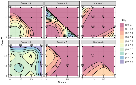
Figure 1: Contour plots showing the utility surface from scenarios 1-6. We also display the grid of discrete dose combination levels (i.e., black dots) with their corresponding (true) utility values whenever these (i.e., the utility values) are above zero.

Scenarios 1, 5 and 6 are designed to be uni-modal whereas scenarios 2, 3 and 4 are designed to be bi-modal and therefore more complex. The goal is to have scenarios with low, medium and high utility values for the target dose combination. Scenario 3 is expected to be particularly challenging. In this scenario, we placed very low utility values in the entire path that stage I is expected to follow given the very low toxicity probability that we established throughout the entire dose-toxicity surface. At the end of stage I, the number of positive efficacy responses is expected to be very low and stage II will start with very little information regarding the potential location of the target dose combination.

In these scenarios, the average DLT rate ranged between 7-17%, the proportion of trials with DLT rates above $\theta_{T}$ and $\theta_{T}+0.1$ was equal to zero, and the proportion of early stoppings for safety was also equal to zero. These results are displayed in Table 1. In terms of the distribution of the recommended (true) utilities, Table 2 shows that the average (true) utilities were close to the (true) utilities of the target dose combinations in all scenarios, showing that our design is able to capture complex uni-modal and bi-modal dose-utility surfaces. These average values were always above those obtained with the AAA design, with differences between 0.06 and 0.01. We observe that the median (true) utilities were also very close to the (true) utility of the target dose combination in all scenarios with practically no differences between the proposed design and the AAA design. One of the most notable differences between the proposed design and the AAA design was found in the 95% confidence intervals of the distribution of recommended (true) utilities. The proposed design yielded, in general, narrower distributions, with notable differences with respect to the AAA design in scenarios 2, 4 and 6. We also see that the average (true) utility of the patients allocated with adaptive randomization was relatively close to the (true) utility of the target dose combination, taking into consideration that the adaptive randomization phase is still a learning part of the design.

In Figure S1 of the supplementary material we display the (empirical) distribution of the recommended optimal dose combinations. We see how the design tends to recommend optimal dose combinations in the region(s) in which the (true) utility is higher. In scenarios 3, we observe a larger dispersion of the recommended optimal dose combinations with respect to the other scenarios, even though the average (true) utility is fairly close to the (true) utility of the target dose combinations. This dispersion is however expected given that this scenarios was designed to have a low number of positive efficacy outcomes.

Table 1: Safety operating characteristics from scenarios 1-6. The table displays the average DLT rate, the percentage of trials with DLT rates above $\theta_{T}$ and $\theta_{T}+0.1$, the percentage of trials stopped following the stage I and stage II safety stopping rules from each scenario.

	Scenario
	1	2	3	4	5	6
Average DLT rate (%)	12	17	7	0	11	10
Percentage of trials with DLT rate above $\theta_{T}$ (%)	0	0	0	0	0	0
Percentage of trials with DLT rate above $\theta_{T}+0.1$ (%)	0	0	0	0	0	0
Percentage of trials stopped early for safety (%)	0	0	0	0	0	0

Table 2: Summary of the distribution of the (true) utility of the recommended optimal dose combinations from scenarios 1-6. The table displays the (true) utility of the target dose combination (TDC) as a reference, the average, median and 95% confidence interval (i.e., percentiles 2.5% and 97.5%) of the distribution of (true) utility of the optimal dose combinations (ODC) recommended by the proposed design, the average, median and 95% confidence interval (i.e., percentiles 2.5 and 97.5) of the distribution of (true) utility of the optimal dose combinations (ODC) recommended by the AAA design, and the average (true) utility of the patients allocated during the adaptive randomization (AR) phase from each scenario.

		Scenario
		1	2	3	4	5	6
Utility of TDC (for reference)		0.68	0.94	0.72	0.98	0.36	0.39
Proposed design	Average	0.65	0.92	0.65	0.93	0.30	0.33
	Median	0.66	0.93	0.72	0.94	0.32	0.34
	95% CI	0.58-0.68	0.81-0.94	0.06-0.72	0.65-0.98	0.19-0.35	0.21-0.38
AAA design	Average	0.62	0.86	0.60	0.89	0.28	0.32
	Median	0.66	0.93	0.72	0.94	0.30	0.33
	95% CI	0.55-0.66	0.40-0.94	0.06-0.72	0.57-0.98	0.16-0.33	0.16-0.35
Average utility of patients allocated during AR phase		0.51	0.52	0.33	0.78	0.24	0.26

3.2 Robustness to deviations between the true underlying marginal models and the working marginal models

In this section we evaluated the performance of the proposed design by changing the true underlying marginal probability models. In other words, the binary toxicity and efficacy data were no longer generated using equations (1) and (2). For this evaluation, we used the same marginal probability of toxicity and efficacy models from Lyu et al. (2019). We note that these marginal probabilities do not include an interaction term modeling synergism between the two drugs following the recommendations of Wang and Ivanova (2005) and the simulation results of Mozgunov et al. (2021) for discrete dose combinations. However, omitting an interaction term will compromise safety of the trial and reduce precision of the estimated MTD contour for continuous dose levels as shown in Tighiouart et al. (2022). We implemented ten out the eleven scenarios evaluated in their publication. We decided not to include scenario 4 (see Figure 5 in Lyu et al. (2019)) because the utility function was not defined for any of the dose combinations contained in the initial space of dose combination and, in this article, we restrict the dose-finding search to the initial space of standardized dose combinations $[0,1]\times[0,1]$. In a second evaluation, we implemented the proposed design in the six scenarios displayed in Figure 1 with lower sample sizes in stages I and II.

Regarding the first assessment (i.e., deviation between the true underlying marginal models and the working marginal models), in Figure 2 we show the (true) utility surfaces for the simulated scenarios. The parameter values used to produce these scenarios are available in Table S2 of the supplementary material.

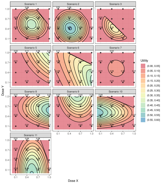
Figure 2: Contour plots showing the (true) utility surface from scenarios 1-3 and 5-11 from Lyu et al. (2019). We also display the grid of discrete dose combination levels (i.e., black dots) with their corresponding (true) utility values whenever these (i.e., the utility values) are above zero.

In terms of safety, the proposed design resulted in an average DLT rate between 13% and 24%, see Table 3. The percentage of trials with DLT rates above $\theta$ ranges between 0.0% and 3.66%, and the percentage of trial with DLT rates above $\theta_{T}+0.1$ were equal to zero. Last, the percentage of trials stopped early for safety ranges between 0% and 2.1%. The safety results published by Lyu et al. (2019) show a worse performance with respect to our proposed design. The most notable difference is visible in scenario 3, where the MTD is located in the middle of the space of dose combinations. In this scenario, AAA design reported a proportion of trials with DLT rate above $\theta_{T}$ was 16.4% whereas in our design this proportion is equal to 3.66%. We would like to highlight that, from our point of view, a proportion of trials with DLT rate above $\theta_{T}$ of 16.4% is too high and more restrictive safety criteria should be applied to lower it.

In terms of the distribution of (true) recommended utilities, the proposed design has an average (true) utility that is, in general, close to the (true) utility of the target dose combinations, with values that are either very similar or higher than those of the AAA design under scenarios 1, 8, 10, and 11. The only scenario in which the proposed design seems to slightly underperform the AAA design is scenario 5. A similar behavior is observed with the medians of the recommended (true) utilities. The 95% confidence interval of the distributions of the (true) utilities are, in general, narrower with the proposed design, with some notable differences under scenarios 1, 2, 8, 10, and 11. These results are consistent with those observed in the main simulation study of this manuscript (see Table 2). We also note that, in the proposed design, the average (true) utility of the patients allocated with adaptive randomization is relatively close to the (true) utility of the target dose combination, taking into consideration that the adaptive randomization phase is still a learning part of the design. These results are displayed in Table 4.

In Figure S2 of the supplementary material we display the distribution of the recommended optimal dose combination in each scenario. Again, this Figure shows how the proposed design correctly identifies the region in which the target dose combination is located. Again, we notice that there is a higher dispersion in the optimal dose combination recommendations in scenarios in which the (true) utility of the target dose combination is, overall, not very high.

Table 3: Safety operating characteristics from scenarios 1-3 and 5-11 from Lyu et al. (2019). The table displays the average DLT rate, the percentage of trials with DLT rates above $\theta_{T}$ of the proposed design, the percentage of trials with DLT rates above $\theta_{T}$ of the AAA design, and $\theta_{T}+0.1$, and the percentage of trials stopped following the stage I and stage II safety stopping rules from each scenario.

	Scenario
	1	2	3	5	6	7	8	9	10	11
Average DLT rate (%) (proposed)	17	16	24	18	19	17	13	13	17	18
Percentage of trials with DLT rate above $\theta_{T}$ (%) (proposed)	0	0	3.66	0.05	0.10	0	0	0	0	0
Percentage of trials with DLT rate above $\theta_{T}$ (%) (AAA)	0	0.1	16.4	0.3	1.3	0	0	0	0	0.1
Percentage of trials with DLT rate above $\theta_{T}+0.1$ (%) (proposed)	0	0	0	0	0	0	0	0	0	0
Percentage of trials stopped early for safety (%) (proposed)	0.25	0.15	0.40	2.10	0.40	0.35	0.10	0.05	0.40	0.85

Table 4: Summary of the distribution of the (true) utility of the recommended optimal dose combinations from scenarios 1-3 and 5-11 from Lyu et al. (2019). The table displays the (true) utility of the target dose combination (TDC) as a reference, the average, median and 95% confidence interval (i.e., percentiles 2.5% and 97.5%) of the distribution of (true) utility of the optimal dose combinations (ODC) recommended by the proposed design, the average, median and 95% confidence interval (i.e., percentiles 2.5 and 97.5) of the distribution of (true) utility of the optimal dose combinations (ODC) recommended by the AAA design, and the average (true) utility of the patients allocated during the adaptive randomization (AR) phase from each scenario.

		Scenario
		1	2	3	5	6	7	8	9	10	11
Utility of TDC (for reference)		0.45	0.55	0.28	0.42	0.47	0.07	0.52	0.46	0.55	0.51
Proposed design	Average	0.42	0.53	0.20	0.26	0.38	0.05	0.46	0.39	0.52	0.48
	Median	0.43	0.54	0.26	0.29	0.45	0.06	0.48	0.42	0.54	0.50
	95% CI	0.35-0.45	0.45-0.55	0.00-0.28	0.01-0.42	0.00-0.47	0.00-0.07	0.21-0.52	0.13-0.46	0.41-0.55	0.40-0.51
AAA design	Average	0.37	0.53	0.20	0.31	0.37	0.04	0.44	0.39	0.46	0.43
	Median	0.34	0.55	0.26	0.33	0.46	0.05	0.45	0.44	0.49	0.44
	95% CI	0.29-0.45	0.29-0.55	0.00-0.28	0.01-0.42	0.00-0.46	0.00-0.07	0.17-0.52	0.14-0.46	0.32-0.53	0.34-0.50
Average utility of patients allocated during AR phase		0.24	0.31	0.12	0.16	0.26	0.03	0.29	0.24	0.31	0.31

3.3 Robustness to changes in the sample size

In this section, we re-assessed the proposed design in the six scenarios generated with the proposed working marginal probability models (i.e., Figure 1) with lower sample sizes in stages I and II. The results are available in Tables S3 and S4 of the supplementary material for sample size of 10, 20, and 30 for stage I, 30, 42, 54, and 66 in stage II, and cohort size 6 and 12 in stage II. Overall, we observed that reducing the number of patients only in stage II yields worse performance than reducing patients only in stage I. We also observed that, for all sample sizes considered in stage I, all scenarios with 54 and 42 patients in stage II had a performance that was still as good as or better than the performance obtained with the AAA design, and the only case in which the proposed design was slightly worse, in some scenarios, than the AAA design, was when stage II uses only 30 patients. In other words, we could enroll 62 patients (i.e., 20 in stage I and 42 in stage II), which would be a 35.42% reduction of the overall sample size, and still have results as good as or better than those from the AAA design.

4 Discussion

We proposed a Bayesian phase I-II design for dual-agent dose optimization with molecularly targeted therapies. Under the presence of these types of compounds, the monotonicity assumption of the dose-efficacy response may not be appropriate given that efficacy may decrease or plateau at high dose levels, and thus the optimal dose will be a trade-off between toxicity and efficacy. For this reason, we employ a flexible cubic spline function for the marginal distribution of the efficacy response and a utility function to assess the risk-benefit trade-off between undesirable and desirable clinical outcomes. The proposed marginal dose-efficacy model has a relatively high number of parameters, which accommodates simple and complex (e.g., bi-modal) dose-efficacy surfaces. However, because in stage I dose-escalation is driven by the marginal dose-toxicity model, which has a small number of parameters, and we do not allow for skipping untried dose combinations, there is no concern regarding the variability of the parameter estimation at the inception of the trial. Then, by the time the design starts using the marginal probability of efficacy to allocate subsequent cohorts of patients, there are already enough patients enrolled in the trial.

Traditionally, in settings in which the assumption of monotonicity of the dose-efficacy holds (i.e., with cytotoxic agents), the purpose was not to have a precise estimation of the entire dose-efficacy curve (or surface) but to provide a precise estimation of the MTD in phase I trials, or the optimal dose in phase I-II trials. However, without the assumption of monotonicity of the dose-efficacy curve (or surface), implementing dose optimization becomes harder since the target dose combination could be anywhere in the space of doses available in the clinical trial and in regions with low probability of toxicity. In this situation, having a more precise estimation of the entire dose-efficacy curve (or surface) could be helpful since we can better locate the region(s) in which the target dose (or dose combination) is located.

We are inspired by a published case study which combines a MEK inhibitor and a PIK3CA inhibitor considering 4 discrete dose levels in each compound and a total of 96 late-stage cancer patients (Lyu et al. (2019)). In this setting, we first implemented our approach using 6 scenarios generated by the working marginal dose-toxicity and dose-efficacy models. These scenarios were intended to have different utility contour shapes, with one or two modes, and with low, medium and high (true) utility values for the target dose combinations. The proposed design achieved good operating characteristics, with low toxicity rates and with average recommended (true) utilities that were close to the (true) utilities of the target dose combinations. In other words, the design was, on average, able to correctly identify the region(s) of the utility surface in which the target dose combination was located.

To assess model robustness to deviations from the true marginal models for toxicity and efficacy, we derived operating characteristics under the scenarios presented in Lyu et al. (2019). The proposed design showed, again, low toxicity rates and average (true) utilities of the recommended optimal dose combination that were close to the (true) utilities of the scenario-specific target dose combinations.

The performance of the proposed design was compared to that of the AAA design, a state-of-the-art design proposed by Lyu et al. (2019) specifically tailored for the combination of molecularly targeted therapies. For this purpose, we implemented the AAA design in the scenarios generated with the working marginal models that we proposed in this article, as well as in the scenarios generated with the marginal models from Lyu et al. (2019). In terms of safety, we have observed that the proposed design is safer than the AAA design, as explained in section 3.2. In terms of target dose combination(s) recommendation, we looked at the distribution of the (true) utilities of the recommended optimal dose combinations produced by both designs. These results showed that, under the presence of more complex (e.g., bi-modal) utility surfaces, the proposed design had better performance (i.e., higher average (true) utility of the recommended optimal dose combinations) than the AAA design. When the surfaces were less complex (e.g., uni-modal), the differences in performance between the proposed design and the AAA design became smaller. The distribution of the (true) utilities of the recommended optimal dose combinations of the proposed design, measured through the percentiles 2.5 and 97.5, were narrower with respect to those from the AAA design, with notable differences in some scenarios. We also evaluated the robustness of the proposed design with respect to smaller sample sizes in stages I and II. This assessment showed that the operating characteristics of the design with smaller sample sizes in both stages were still close to those obtained with the sample size used for the main simulation study. As a reference, we observed that an overall sample size reduction of 35% still leads to operating characteristics that were as good as or better than those produced by the AAA design in the evaluated scenarios. With these results, we conclude that the number of parameters employed by the marginal probability of efficacy model is not an issue in this type of clinical trial setting.

In general, we believe that the proposed design has the following advantages over the AAA design: i) it has better safety operating characteristics, ii) it has better performance, specially under complex dose-utility surfaces, iii) it is more precise in terms of optimal dose combination recommendation, and iv) it is easier to implement since it does not incorporate the adaptive dose insertion feature of the AAA design, which could be challenging in practice if many dose insertions are needed during the trial. One potential weakness of the proposed design has been observed in the scenarios in which the (true) utility surface had, overall, low values. In this setting, there was a slightly higher dispersion of the optimal dose combination recommendation with respect to other tested scenarios, which translated into slightly lower average (true) utilities. However, a higher dispersion in this situation was not completely unexpected since low utility values are usually a result of low efficacy rates, which, given the relatively high number of parameter of the marginal efficacy model, can lead to lower estimation precision. Nevertheless, because we are using vague prior distributions, we can consider the results presented in this manuscript as the baseline operating characteristics of the proposed design. By using more informative prior distributions in the marginal probability models, and/or increasing the sample size, the design’s operating characteristics are expected to improve.

Data availability

No real data was used in the development of this article. The R and JAGS scripts necessary to fully reproduce the results presented in this article are available at
https://github.com/jjimenezm1989/Phase-I-II-design-targeted-therapies.

Funding

Mourad Tighiouart is funded by NIH the National Center for Advancing Translational Sciences (NCATS) UCLA CTSI (UL1 TR001881-01), NCI P01 CA233452-02, and U01 grant CA232859-01.

Disclaimer

José L. Jiménez is employed by Novartis Pharma A.G. who provided support in the form of salary for the author, but did not have any additional role in the preparation of the manuscript. Also, the views expressed in this publication are those of the authors and should not be attributed to any of the funding institutions or organisations to which the authors are affiliated.

References

- Babb et al. [1998] James Babb, André Rogatko, and Shelemyahu Zacks. Cancer phase I clinical trials: efficient dose escalation with overdose control. Statistics in Medicine, 17(10):1103–1120, 1998.
- Cai et al. [2014] Chunyan Cai, Ying Yuan, and Yuan Ji. A Bayesian dose-finding design for oncology clinical trials of combinational biological agents. Journal of the Royal Statistical Society. Series C, Applied statistics, 63(1):159, 2014.
- Diniz et al. [2017] Márcio Augusto Diniz, Quanlin Li, and Mourad Tighiouart. Dose finding for drug combination in early cancer phase I trials using conditional continual reassessment method. Journal of Biometrics & Biostatistics, 8(6), 2017.
- Diniz et al. [2018] Márcio Augusto Diniz, Sungjin Kim, and Mourad Tighiouart. A Bayesian adaptive design in cancer phase I trials using dose combinations in the presence of a baseline covariate. Journal of Probability and Statistics, 2018, 2018.
- Diniz et al. [2019] Márcio Augusto Diniz, Mourad Tighiouart, and André Rogatko. Comparison between continuous and discrete doses for model based designs in cancer dose finding. PLoS One, 14(1):e0210139, 2019.
- Guo and Yuan [2015] Beibei Guo and Ying Yuan. A Bayesian dose-finding design for phase I/II clinical trials with nonignorable dropouts. Statistics in Medicine, 34(10):1721–1732, 2015.
- Guo and Yuan [2017] Beibei Guo and Ying Yuan. Bayesian phase I/II biomarker-based dose finding for precision medicine with molecularly targeted agents. Journal of the American Statistical Association, 112(518):508–520, 2017.
- Hoff and Ellis [2007] Paulo M Hoff and Lee M Ellis. Targeted therapy trials: Approval strategies, target validation, or helping patients? Journal of Clinical Oncology, 25(13):1639–1641, 2007.
- Houede et al. [2010] Nadine Houede, Peter F Thall, Hoang Nguyen, Xavier Paoletti, and Andrew Kramar. Utility-based optimization of combination therapy using ordinal toxicity and efficacy in phase I/II trials. Biometrics, 66(2):532–540, 2010.
- Ivanova et al. [2009] Anastasia Ivanova, Ken Liu, Ellen Snyder, and Duane Snavely. An adaptive design for identifying the dose with the best efficacy/tolerability profile with application to a crossover dose-finding study. Statistics in Medicine, 28(24):2941–2951, 2009.
- Jiménez and Tighiouart [2022] José L Jiménez and Mourad Tighiouart. Combining cytotoxic agents with continuous dose levels in seamless phase I-II clinical trials. Journal of the Royal Statistical Society: Series C (Applied Statistics), in print, 2022.
- Jiménez and Zheng [2021] José L Jiménez and Haiyan Zheng. A Bayesian adaptive design for dual-agent phase I-II cancer clinical trials combining efficacy data across stages. arXiv preprint, 2021.
- Jimenez et al. [2019] Jose L Jimenez, Mourad Tighiouart, and Mauro Gasparini. Cancer phase I trial design using drug combinations when a fraction of dose limiting toxicities is attributable to one or more agents. Biometrical Journal, 61(2):319–332, 2019.
- Jiménez et al. [2020] José L Jiménez, Sungjin Kim, and Mourad Tighiouart. A bayesian seamless phase I–II trial design with two stages for cancer clinical trials with drug combinations. Biometrical Journal, 62(5):1300–1314, 2020.
- Le Tourneau et al. [2009] Christophe Le Tourneau, J Jack Lee, and Lillian L Siu. Dose escalation methods in phase I cancer clinical trials. JNCI: Journal of the National Cancer Institute, 101(10):708–720, 2009.
- Li et al. [2017] Daniel H Li, James B Whitmore, Wentian Guo, and Yuan Ji. Toxicity and efficacy probability interval design for phase I adoptive cell therapy dose-finding clinical trials. Clinical Cancer Research, 23(1):13–20, 2017.
- Lin et al. [2020] Ruitao Lin, Peter F Thall, and Ying Yuan. An adaptive trial design to optimize dose-schedule regimes with delayed outcomes. Biometrics, 76(1):304–315, 2020.
- Liu et al. [2018] Suyu Liu, Beibei Guo, and Ying Yuan. A Bayesian phase I/II trial design for immunotherapy. Journal of the American Statistical Association, 113(523):1016–1027, 2018.
- Lyu et al. [2019] Jiaying Lyu, Yuan Ji, Naiqing Zhao, and Daniel VT Catenacci. AAA: triple adaptive Bayesian designs for the identification of optimal dose combinations in dual-agent dose finding trials. Journal of the Royal Statistical Society. Series C, Applied statistics, 68(2):385, 2019.
- Mozgunov et al. [2021] Pavel Mozgunov, R Knight, H Barnett, and Thomas Jaki. Using an interaction parameter in model-based phase i trials for combination treatments? a simulation study. Int J Environ Res Public Health, 18(1):345, 2021.
- Murray et al. [2017] Thomas A Murray, Peter F Thall, Ying Yuan, Sarah McAvoy, and Daniel R Gomez. Robust treatment comparison based on utilities of semi-competing risks in non-small-cell lung cancer. Journal of the American Statistical Association, 112(517):11–23, 2017.
- Nebiyou Bekele and Shen [2005] B Nebiyou Bekele and Yu Shen. A Bayesian approach to jointly modeling toxicity and biomarker expression in a phase I/II dose-finding trial. Biometrics, 61(2):343–354, 2005.
- Plummer et al. [2003] Martyn Plummer et al. Jags: A program for analysis of Bayesian graphical models using gibbs sampling. In Proceedings of the 3rd international workshop on distributed statistical computing, volume 124, pages 1–10. Vienna, Austria., 2003.
- R Core Team [2019] R Core Team. R: A Language and Environment for Statistical Computing. R Foundation for Statistical Computing, Vienna, Austria, 2019. URL https://www.R-project.org/.
- Shi and Yin [2013] Yun Shi and Guosheng Yin. Escalation with overdose control for phase I drug-combination trials. Statistics in Medicine, 32(25):4400–4412, 2013.
- Thall and Cook [2004] Peter F Thall and John D Cook. Dose-finding based on efficacy-toxicity trade-offs. Biometrics, 60(3):684–693, 2004.
- Thall et al. [2013] Peter F Thall, Hoang Q Nguyen, Thomas M Braun, and Muzaffar H Qazilbash. Using joint utilities of the times to response and toxicity to adaptively optimize schedule–dose regimes. Biometrics, 69(3):673–682, 2013.
- Thall et al. [2014] Peter F Thall, Hoang Q Nguyen, Sarah Zohar, and Pierre Maton. Optimizing sedative dose in preterm infants undergoing treatment for respiratory distress syndrome. Journal of the American Statistical Association, 109(507):931–943, 2014.
- Tighiouart [2019] Mourad Tighiouart. Two-stage design for phase I–II cancer clinical trials using continuous dose combinations of cytotoxic agents. Journal of the Royal Statistical Society: Series C (Applied Statistics), 68(1):235–250, 2019.
- Tighiouart and Rogatko [2010] Mourad Tighiouart and André Rogatko. Dose finding with escalation with overdose control (EWOC) in cancer clinical trials. Statistical Science, 25(2):217–226, 2010.
- Tighiouart and Rogatko [2012] Mourad Tighiouart and Andre Rogatko. Number of patients per cohort and sample size considerations using dose escalation with overdose control. Journal of Probability and Statistics, 2012, 2012.
- Tighiouart et al. [2005] Mourad Tighiouart, André Rogatko, and James S Babb. Flexible Bayesian methods for cancer phase I clinical trials. dose escalation with overdose control. Statistics in Medicine, 24(14):2183–2196, 2005.
- Tighiouart et al. [2014] Mourad Tighiouart, Steven Piantadosi, and André Rogatko. Dose finding with drug combinations in cancer phase I clinical trials using conditional escalation with overdose control. Statistics in Medicine, 33(22):3815–29, 2014.
- Tighiouart et al. [2017] Mourad Tighiouart, Quanlin Li, and André Rogatko. A Bayesian adaptive design for estimating the maximum tolerated dose curve using drug combinations in cancer phase I clinical trials. Statistics in Medicine, 36(2):280–290, 2017.
- Tighiouart et al. [2022] Mourad Tighiouart, José L Jiménez, Marcio A Diniz, and André Rogatko. Tmodeling synergism in early phase cancer trials with drug combination with continuous dose levels: is there an added value? Brazilian Journal of Biometrics, in print, 2022.
- Wang and Ivanova [2005] Kai Wang and Anastasia Ivanova. Two-dimensional dose finding in discrete dose space. Biometrics, 61(1):217–222, 2005.
- Wheeler et al. [2017] Graham M Wheeler, Michael J Sweeting, and Adrian P Mander. Toxicity-dependent feasibility bounds for the escalation with overdose control approach in phase I cancer trials. Statistics in Medicine, 36(16):2499–2513, 2017.
- Yuan and Yin [2011] Ying Yuan and Guosheng Yin. Bayesian phase I/II adaptively randomized oncology trials with combined drugs. The Annals of Applied Statistics, 5(2A):924, 2011.
- Yuan et al. [2016] Ying Yuan, Hoang Q Nguyen, and Peter F Thall. Bayesian designs for phase I–II clinical trials. CRC Press, 2016.
- Zhang et al. [2006] Wei Zhang, Daniel J Sargent, and Sumithra Mandrekar. An adaptive dose-finding design incorporating both toxicity and efficacy. Statistics in Medicine, 25(14):2365–2383, 2006.