Quantum annealing with error mitigation

Abstract

Quantum annealing (QA) is one of the efficient methods to calculate the ground-state energy of a problem Hamiltonian. In the absence of noise, QA can accurately estimate the ground-state energy if the adiabatic condition is satisfied. However, in actual physical implementation, systems suffer from decoherence. On the other hand, much effort has been paid into the noisy intermediate-scale quantum (NISQ) computation research. For practical NISQ computation, many error mitigation (EM) methods have been devised to remove noise effects. In this paper, we propose a QA strategy combined with the EM method called dual-state purification to suppress the effects of decoherence. Our protocol consists of four parts; the conventional dynamics, single-qubit projective measurements, Hamiltonian dynamics corresponding to an inverse map of the first dynamics, and post-processing of measurement results. Importantly, our protocol works without two-qubit gates, and so our protocol is suitable for the devices designed for practical QA. We also provide numerical calculations to show that our protocol leads to a more accurate estimation of the ground energy than the conventional QA under decoherence.

I Introduction

Quantum annealing (QA) Kadowaki and Nishimori (1998); Farhi et al. (2000, 2001) is a promising way to obtain a ground state of a problem Hamiltonian. Initially, the system is prepared as a ground state of a driver Hamiltonian. In QA, we adopt a time-dependent total Hamiltonian that changes from the driver Hamiltonian to the problem Hamiltonian, and we let the state evolve by such a Hamiltonian. As long as the adiabatic condition is satisfied, we obtain the ground state of the problem Hamiltonian after the dynamics without noise Ehrenfest (1916); Kato (1950); Amin (2009); Dodin and Brumer (2021).

We can obtain the ground state of the Ising-type problem Hamiltonian by measuring the state after QA in the computational basis, as long as the state has a finite population of the ground state Lechner et al. (2015); Kumar et al. (2018); Choi (2011). The density matrix after the QA can be expanded by the energy eigenbasis as $\rho=\sum_{j,j^{\prime}}d_{j,j^{\prime}}\ket{E_{j}}\bra{E_{j^{\prime}}}$ where $d_{j,j^{\prime}}$ denotes a coefficient, $p_{j}\equiv d_{j,j}$ denotes a population, and $\ket{E_{j}}$ denotes an eigenvector of the problem Hamiltonian. In this case, the probability to obtain the ground state with the measurement in the computational basis is described by $1-(1-p_{0})^{N_{\rm{trial}}}$ where $p_{0}$ denotes the population of the ground state and $N_{\rm{trial}}$ denotes the number of trials. Thus, we can obtain the ground state after many trials as long as $p_{0}$ has a non-zero value.

On the other hand, when the problem Hamiltonian contains non-diagonal elements, the main aim is to estimate the energy of the ground state, which is the focus of our paper. For such a Hamiltonian, we cannot obtain the ground state of the problem Hamiltonian by the measurements in the computational basis after QA. The expectation value of the problem Hamiltonian with the density matrix $\rho$ after QA is given as $\expectationvalue{H_{\rm{P}}}=\mathrm{Tr}[H_{\rm{P}}\rho]=\sum_{j}p_{j}E_{j}$. The problem Hamiltonian $H_{\mathrm{P}}$ can be expanded by the products of the Pauli matrices such as $H_{\mathrm{P}}=\sum_{i}c_{i}\sigma_{i}$ where $c_{i}$ denotes a coefficient and $\sigma_{i}$ denotes a Pauli product. To obtain the expectation value of the problem Hamiltonian, one needs to know the expectation value of each term by the measurements in the Pauli basis after QA and take the summation of these expectation values. Notably, a finite population of the excited state after QA leads to an error in the estimation of the ground-state energy. Therefore, for accurate estimation of the ground-state energy, we need to prepare the ground state with high fidelity.

However, QA suffers from non-adiabatic transitions and decoherence Morita and Nishimori (2008); Albert (1961, 1962); Roland and Cerf (2005); Åberg et al. (2005); Albash and Lidar (2015); Childs et al. (2001); Sarandy and Lidar (2005). If the dynamics are not slow enough to satisfy the adiabatic condition, unwanted transitions from the ground state to the excited states occur. On the other hand, if the time scale of QA is comparable with or larger than the coherence time of the qubit, the system is affected by decoherence, which also induces unwanted transitions to the excited states. Thus, the estimation of the ground energy would be biased, as shown in Fig. 1 (a).

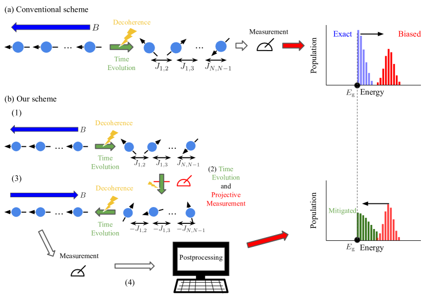
Figure 1: The conceptual diagram to indicate the difference between the conventional and our schemes in QA. (a) With the conventional scheme, one gradually changes the total Hamiltonian from a driver Hamiltonian $H_{\mathrm{D}}$ to a problem Hamiltonian $H_{\mathrm{P}}$. The blue bars in the graph draw the exact populations without decoherence which can include the effects of non-adiabatic transitions. By decoherence, we actually obtain the biased populations as shown by the red bars. In this case, the estimation of the ground-state energy $E_{\mathrm{g}}$ of $H_{\mathrm{P}}$ should be inaccurate if there is decoherence. (b) With our scheme to incorporate the EM method, there are four parts: (1) the conventional dynamics, (2) switching the sign of the coefficients in $H_{\mathrm{P}}$ and single-qubit projective measurements, (3) Hamiltonian dynamics corresponding to an inverse map of the first dynamics, and (4) post-processing the measurement results. The green bars illustrate the populations in which noise effects are mitigated. Due to the EM method, we can estimate the ground-state energy more accurate than the conventional QA in Fig. 1 (a).

Meanwhile, many research works have been devoted theoretically and experimentally to realizing practical noisy intermediate-scale quantum (NISQ) computing Preskill (2018); Endo et al. (2021); Cerezo et al. (2021). We can use NISQ devices to perform quantum computation using tens to thousands of qubits, with $10^{-3}$ or lower gate errors. Many algorithms for NISQ computing have been proposed. Here, variational quantum circuits are typically used to generate a trial wave function to minimize a cost function Peruzzo et al. (2014); Li and Benjamin (2017); McClean et al. (2016); Yuan et al. (2019); Endo et al. (2020). In these algorithms, one needs to measure observables on the qubits corresponding to the trial wave function. In the actual devices, noise prevents one from obtaining the accurate expectation values of the observable, degrading the algorithm performance. Fortunately, sophisticated techniques called “error mitigation” (EM) suppress the effect of noise by implementing additional quantum gates and post-processing with classical computation Endo et al. (2021); Li and Benjamin (2017); Kandala et al. (2019); Temme et al. (2017); Endo et al. (2018); Song et al. (2019); Zhang et al. (2020); McArdle et al. (2019); Bonet-Monroig et al. (2018); Sun et al. (2021); LaRose et al. (2022); Quantum et al. (2020); McClean et al. (2017); Merkel et al. (2013); Stark (2014); Greenbaum (2015); Blume-Kohout et al. (2017); Strikis et al. (2021); Czarnik et al. (2021a); Wang et al. (2021); O’Brien et al. (2021); Yoshioka et al. (2022); Cai et al. (2022); Cao et al. (2022).

There are many types of EM. The quasi-probability method is one way to mitigate the environmental effect Temme et al. (2017); Endo et al. (2018); Huo and Li (2021); Takagi (2021); Song et al. (2019); Zhang et al. (2020); Hakoshima et al. (2021); Sun et al. (2021); Suzuki et al. (2022). By applying stochastic operations during the implementation of the quantum algorithm, one can effectively cancel out the environmental noise. However, this method requires accurate information about the noise model. If the environmental noise model does not change during the experiments, a so-called gate set tomography allows us to know the noise model with the considerable measurement cost. If the noise model changes in time, the quasi-probability methods cannot mitigate noise effects.

On the other hand, the virtual distillation (VD) method, which is also known as the exponential error suppression (EES) method, can mitigate the error without knowing the detail of the noise model Koczor (2021); Huggins et al. (2021); Czarnik et al. (2021b); Yamamoto et al. (2021). Suppose that $N$ qubits are required to implement a quantum algorithm without EM. In VD/EES, one needs to prepare $M$ copies of noisy quantum states $\rho$ composed of $N$ qubits to mitigate the error. We assume that these states are generated by the same quantum circuit and influenced by the same noise model. Via the implementation of entangling gates between $M$ copies of a quantum state $\rho$, one can obtain $\expectationvalue{O}^{(M)}_{\mathrm{VD}}=\mathrm{Tr}[O\rho^{(M)}_{\mathrm{VD}}]$ with $\rho^{(M)}_{\mathrm{VD}}=\rho^{M}/\mathrm{Tr}[\rho^{M}]$. The advantage of this scheme is that the population of the dominant eigenvector of $\rho$ approaches unity, and so stochastic errors are exponentially suppressed as one increases $M$. However, VD/EES requires $MN$ qubits of the quantum state, and this is costly for NISQ computers.

Recently, to overcome this problem, an alternative scheme called “dual-state purification” was proposed Huo and Li (2022). Let us consider the specific case $M=2$. In this scheme, one can effectively prepare two copies of the quantum state on the same qubits. one can physically generate one of them in an original quantum circuit, while the other one can be virtually prepared by the use of an inverse of the original circuit, which is designed to be the conjugate transpose of the original circuit when there is no error. By decomposing an observable $O$ into Pauli products $\{\sigma_{i}\}$, one obtains the expectation value $\expectationvalue{O}$ as $\Sigma a_{i}\expectationvalue{\sigma_{i}}$ where $a_{i}$ is a coefficient. In dual-state purification, one calculates each expectation value $\expectationvalue{\sigma_{i}}$ with each corresponding circuit and then takes the summation to compute the expectation value $\expectationvalue{O}$. The entire circuit for dual-state purification is composed of the original circuit, the projective measurement of a Pauli product $\sigma_{i}$, the inverse circuit, and the projective measurement to the initial state. After post-processing operations with classical computation, one obtains the expectation value of $O$, where stochastic errors during the implementation of quantum circuits are mitigated. Importantly, this scheme requires only $N$ qubits.

In this paper, we propose QA with dual-state purification. With naive applications of dual-state purification to QA, the use of the so-called reverse quantum annealing seems to be promising for the construction of the inverse dynamics of QA. More specifically, the conventional QA is firstly performed where we gradually decrease (increase) the driver (problem) Hamiltonian, projective measurements are performed, and then the reverse QA is implemented where we gradually increase (decrease) the driver (problem) Hamiltonian. However, we show that this strategy could fail to estimate the ground-state energy, and dual-state purification provides an unphysical density matrix with negative eigenvalues. To overcome this problem, we propose modified scheduling to apply dual-state purification to QA. As shown in Fig. 1 (b), (1) we perform the same dynamics as the conventional QA, (2) we change the sign of the problem Hamiltonian in an adiabatic way and perform single-qubit projective measurements, (3) we gradually decrease (increase) the driver (problem) Hamiltonian, and (4) we post-process measurement results. In this case, we show that the density matrix produced by dual-state purification does not have negative eigenvalues. Moreover, we numerically demonstrate that our strategy provides a more accurate estimation than the conventional QA.

II Quantum annealing

Let us review QA to obtain the ground state and the ground-state energy of a problem Hamiltonian $H_{\mathrm{P}}$ Kadowaki and Nishimori (1998); Farhi et al. (2000, 2001). We choose the independent spin model with the transverse field (i.e., $H_{\mathrm{D}}=-B\sum^{N}_{i=1}\hat{\sigma}^{x}_{i}$) as a driver Hamiltonian where $N$ denotes the number of qubits and $B$ denotes a coefficient. Also, the system is initially prepared as $\ket{+}^{\otimes N}$ which is the ground state of the driver Hamiltonian $H_{\mathrm{D}}$ where $\ket{+}=\frac{1}{\sqrt{2}}(\ket{0}+\ket{1})$ denotes the eigenstate of $\hat{\sigma}^{x}$ and $\ket{0}$ and $\ket{1}$ denote the eigenstates of $\hat{\sigma}^{z}$. We change the total Hamiltonian $H(t)$ from the driver Hamiltonian $H_{\mathrm{D}}$ to the problem Hamiltonian $H_{\mathrm{P}}$ over time as

$$H(t)=A_{t}H_{\mathrm{P}}+B_{t}H_{\mathrm{D}},$$ (1)

where $A_{t}$ and $B_{t}$ are the time-dependent coefficients. The coefficients of the total Hamiltonian in QA are given by

$$A_{t}=\dfrac{t}{T}\ (t:0\rightarrow T),$$

$$B_{t}=1-\dfrac{t}{T}\ (t:0\rightarrow T),$$

where $T$ is the annealing time (see Fig. 2). If the total Hamiltonian $H(t)$ is varied sufficiently slowly, the adiabatic theorem guarantees that we can obtain the ground state of $H_{\mathrm{P}}$.

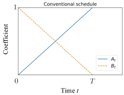
Figure 2: The schedule of the conventional QA. $A_{t}$ ($B_{t}$) represents the coefficient of a problem Hamiltonian $H_{\mathrm{P}}$ (a driver Hamiltonian $H_{\mathrm{D}}$). We linearly change $A_{t}$ ($B_{t}$) from $0$ to $1$ (from $1$ to $0$) for an annealing time $T$.

In estimating the ground-state energy by QA, there are two main problems: environmental decoherence and non-adiabatic transitions Morita and Nishimori (2008); Albert (1961, 1962); Roland and Cerf (2005); Åberg et al. (2005); Albash and Lidar (2015); Childs et al. (2001); Sarandy and Lidar (2005). If we perform QA with a longer time schedule, we can avoid the effect of non-adiabatic transitions. However, the longer time schedule makes quantum states more fragile against decoherence. This trade-off relation leads to the difficulty to solve practical problems with QA.

There are many types of research to suppress the non-adiabatic transitions and decoherence during QA. Inhomogeneous driver Hamiltonian can be used to accelerate QA for a specific problem Hamiltonian Susa et al. (2018a, b). Seki et al. show that the performance of QA for certain types of problem Hamiltonian can be improved with ”non-stoquastic” Hamiltonians that have negative off-diagonal matrix elements Seki and Nishimori (2012, 2015). It is known that the energy gap between the ground state and the first excited state can be estimated in a robust way against non-adiabatic transitions Matsuzaki et al. (2021); Mori et al. (2022). Moreover, there are several works to suppress environmental noise. An error correction with ancillary qubits can be adopted to suppress decoherence during QA Pudenz et al. (2014). A scheme with a decoherence-free subspace for QA is also known Suzuki and Nakazato (2020). Spin lock techniques are beneficial to use long-lived qubits for QA Chen et al. (2011); Nakahara (2013); Matsuzaki et al. (2020). In addition, there are several schemes to improve the performance of QA by using non-adiabatic transitions and quenching Crosson et al. (2014); Goto and Kanao (2020); Hormozi et al. (2017); Muthukrishnan et al. (2016); Brady and van Dam (2017); Somma et al. (2012); Das and Chakrabarti (2008); Karanikolas and Kawabata (2020) and degenerating two-level systems Watabe et al. (2020). Variational methods have also been applied to QA to suppress non-adiabatic transitions and decoherence Susa and Nishimori (2021); Matsuura et al. (2021); Passarelli et al. (2021); Imoto et al. (2021).

III Dual-state purification

In this section, we review the EM method called dual-state purification Huo and Li (2022). Firstly, we introduce VD/EES methods for NISQ devices in this paragraph which dual-state purification is based on. In the VD/EES methods Koczor (2021); Huggins et al. (2021); Czarnik et al. (2021b), by using two copies of a noisy state $\rho$, we obtain a purified state $\rho_{\rm{VD/EES}}^{(2)}=\rho^{2}/\mathrm{Tr}[\rho^{2}]$. Let us assume that the state is written by orthogonal basis as $\rho=\sum_{n=0}^{2^{N}-1}p_{n}|\psi_{n}\rangle\langle\psi_{n}|$ where $|\psi_{0}\rangle=U|\vec{\mathbb{0}}\rangle$ denotes the ideal state, $U$ is a unitary operator without any noise, and $\ket*{\vec{\mathbb{0}}}$ denotes an initial state. In this case, the purified state $\rho_{\rm{VD/EES}}^{(2)}$ is closer to the ideal state than the original state for $p_{0}>1/2$. The expectation value of an observable $O$ is estimated as $\expectationvalue{O}=\bra{\psi_{0}}O\ket{\psi_{0}}\simeq\mathrm{Tr}[O\rho^{2}]/\mathrm{Tr}[\rho^{2}]$. However, in this scheme, the necessary number of qubits becomes twice larger than that of the original scheme without VD/EES methods.

Let us review another EM scheme called dual-state purification that can be implemented by the same number of the qubits as the original scheme Huo and Li (2022). To implement the dual-state purification, we consider a noisy map $\mathcal{F}(\bullet)=\sum_{k}F_{k}\bullet F_{k}^{\dagger}$ where $\{F_{i}\}$ denote Kraus operators. When the noise amplitude is significantly small, this map is close to the ideal unitary operator $U$ (i.e., $\mathcal{F}(\bullet)\simeq U\bullet U^{\dagger}$). Let us consider a quantum process corresponding to the inverse quantum operation $U^{{\dagger}}$ if there is no decoherence. We denote the quantum process with noise as $\mathcal{G}(\bullet)=\sum_{k}G_{k}\bullet G_{k}^{\dagger}$ where $\{G_{i}\}$ also denote Kraus operators. If the noise effect can be ignored, this noisy map $\mathcal{G}(\bullet)$ can be approximated as $U^{\dagger}\bullet U$.

By using these operations $\mathcal{F}$ and $\mathcal{G}$, we obtain

$$\bra*{\vec{\mathbb{0}}}\mathcal{G}\left(\mathcal{F}(\outerproduct*{\vec{\mathbb{0}}}{\vec{\mathbb{0}}})\right)\ket*{\vec{\mathbb{0}}}$$ (2)

$$= \mathrm{Tr}[\bar{\mathcal{G}}(\outerproduct*{\vec{\mathbb{0}}}{\vec{\mathbb{0}}})\mathcal{F}(\outerproduct*{\vec{\mathbb{0}}}{\vec{\mathbb{0}}})]=\mathrm{Tr}[\bar{\rho}\rho],$$

where $\bar{\mathcal{G}}(\bullet)=\sum_{k}G_{k}^{\dagger}\bullet G_{k}$ and $\bar{\rho}=\bar{\mathcal{G}}(\outerproduct*{\vec{\mathbb{0}}}{\vec{\mathbb{0}}})$. We call $\bar{\mathcal{G}}$ the dual map of $\mathcal{G}$, while we call $\bar{\rho}$ the dual state. We can obtain $\bar{\mathcal{G}}(\bullet)\simeq U\bullet U^{\dagger}$ and $\mathrm{Tr}[\bar{\rho}\rho]\simeq\mathrm{Tr}[\rho^{2}]$ when the noise strength is sufficiently small.

Let us show how dual-state purification increases the population of the ideal state $\ket{\psi_{0}}$. In this paragraph, we assume $\rho=(1-p)\outerproduct*{\psi_{0}}{\psi_{0}}+p\rho_{e}$ and $\bar{\rho}=(1-\bar{p})\outerproduct*{\psi_{0}}{\psi_{0}}+\bar{p}\bar{\rho}_{e}$ where $\rho_{e}$ ($\bar{\rho}_{e}$) denotes a normalized positive-semidefinite state and $p$ ($\bar{p}$) denotes an error probability to satisfy $1-p>p$ ($1-\bar{p}>\bar{p}$). Also we assume incoherent errors where the state $\rho_{e}$ ($\bar{\rho}_{e}$) satisfies $\outerproduct*{\psi_{0}}{\psi_{0}}\rho_{e}=0$ ($\outerproduct*{\psi_{0}}{\psi_{0}}\bar{\rho}_{e}=0$) Koczor (2021); Huggins et al. (2021). The virtually purified state without normalization is defined as follows:

$$\dfrac{\rho\bar{\rho}+\bar{\rho}\rho}{2}=(1-p)(1-\bar{p})\outerproduct*{\psi_{0}}{\psi_{0}}+p\bar{p}\ \mathrm{Tr}[\rho_{e}\bar{\rho}_{e}]\dfrac{\rho_{e}\bar{\rho}_{e}+\bar{\rho}_{e}\rho_{e}}{2\mathrm{Tr}[\rho_{e}\bar{\rho}_{e}]},$$ (3)

where the state $\rho\bar{\rho}+\bar{\rho}\rho$ is Hermitian. Note that this EM method decreases the ratio between the error state and the ideal state from $p/(1-p)$ and $\bar{p}/(1-\bar{p})$ to $p\bar{p}\ \mathrm{Tr}[\rho_{e}\bar{\rho}_{e}]/(1-p)(1-\bar{p})\leq p\bar{p}/(1-p)(1-\bar{p})$. By considering the state $\rho\bar{\rho}+\bar{\rho}\rho$, this EM method can effectively improve the population of the ideal state without the information of the noise model unlike previous schemes such as the quasi-probability method.

We obtain the expectation value of an observable $O$ as $\expectationvalue{O}=\Sigma a_{i}\expectationvalue{\sigma_{i}}$ by decomposing $O$ as the summation of the expectation values of Pauli products $\{\sigma_{i}\}$ where $a_{i}$ is a coefficient. Dual-state purification gives the expectation value of a Pauli product $\sigma$ as

$$\expectationvalue{\sigma}\simeq\left.\mathrm{Tr}\left[\sigma\dfrac{\rho\bar{\rho}+\bar{\rho}\rho}{2}\right]\middle/\mathrm{Tr}\left[\dfrac{\rho\bar{\rho}+\bar{\rho}\rho}{2}\right]\right.$$ (4)

where $\mathrm{Tr}\left[\dfrac{\rho\bar{\rho}+\bar{\rho}\rho}{2}\right]$ denotes a normalization factor. To obtain this expectation value, we can implement quantum circuits described in Fig. 3. We perform the circuit in Fig. 3 (Fig. 3) to obtain the numerator (the denominator) in Eq. (4). First, prepare an initial state $\ket*{\vec{\mathbb{0}}}$, and let this state evolve by the noisy quantum circuit described by the channel $\mathcal{F}$. Second, perform a projective measurement $P_{\sigma}^{\pm}$ of a Pauli product $\sigma$ for the numerator as shown in Fig. 3 where the measurement operator corresponding to the outcome $\pm 1$ is given by $P_{\sigma}^{\pm}=(I\pm\sigma)/2$. When we implement the circuit in Fig. 3 to obtain the denominator in Eq. (4), we do not perform the projective measurement. Third, let the state evolve by the noisy quantum process described by the channel $\mathcal{G}$. Finally, we investigate how much population remains in $\ket*{\vec{\mathbb{0}}}$ by a measurement in the basis including $\ket*{\vec{\mathbb{0}}}$. If we choose the circuit in Fig. 3, we can measure the denominator in Eq. (4) as follows:

$$P_{\vec{\mathbb{0}}}=\bra*{\vec{\mathbb{0}}}\mathcal{G}\left(\mathcal{F}(\outerproduct*{\vec{\mathbb{0}}}{\vec{\mathbb{0}}})\right)\ket*{\vec{\mathbb{0}}}=\mathrm{Tr}[\bar{\rho}\rho],$$ (5)

where $P_{\vec{\mathbb{0}}}$ denotes the population of $\ket*{\vec{\mathbb{0}}}$ in the final state obtained by the measurement. On the other hand, if we choose the circuit in Fig. 3, we can measure the numerator in Eq. (4) as $\tilde{P}_{\vec{\mathbb{0}}}^{+}-\tilde{P}_{\vec{\mathbb{0}}}^{-}$ where

$$\tilde{P}_{\vec{\mathbb{0}}}^{\pm}=\bra*{\vec{\mathbb{0}}}\mathcal{G}\left(P_{\sigma}^{\pm}\mathcal{F}(\outerproduct*{\vec{\mathbb{0}}}{\vec{\mathbb{0}}})P_{\sigma}^{\pm}\right)\ket*{\vec{\mathbb{0}}}=\mathrm{Tr}[P_{\sigma}^{\pm}\rho P_{\sigma}^{\pm}\bar{\rho}],$$ (6)

$\tilde{P}_{\vec{\mathbb{0}}}^{\pm}$ also denote the population of $\ket*{\vec{\mathbb{0}}}$. To sum up, the expectation value is rewritten by

$$\expectationvalue{\sigma}=(\tilde{P}_{\vec{\mathbb{0}}}^{+}-\tilde{P}_{\vec{\mathbb{0}}}^{-})/P_{\vec{\mathbb{0}}}.$$ (7)

In EM, we also need to suppress the sampling noise which leads to the residual error. We can decrease the variance of the expectation value in Eq. (7) by increasing the number of measurements. Due to the denominator, the variance of Eq. (7) is larger than that of Eq. (6). Especially, when $\mathrm{Tr}[\bar{\rho}\rho]$ approaches to $0$, the variance diverges to an infinity. So, in order to implement our scheme within a finite time, we need a finite value of $\mathrm{Tr}[\bar{\rho}\rho]$.

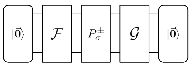
(a)

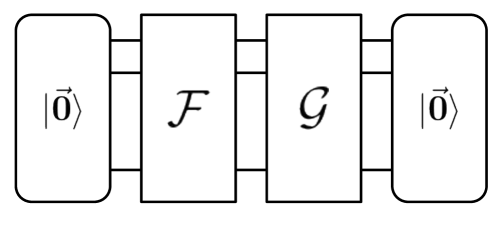
(b)

Figure 3: The circuits for implementing dual-state purification. We calculate the numerator (the denominator) in Eq. (4) with the circuit in Fig. 3 (Fig. 3). First, we perform a noisy map $\mathcal{F}$ in Eq. (2) to an initial state $\ket*{\vec{\mathbb{0}}}$. Second, when we calculate the numerator in Eq. (4), we perform the projective measurement $P_{\sigma}^{\pm}$ of a Pauli product $\sigma$ as shown in Fig. 3. For obtaining the denominator in Eq. (4) by the circuit in Fig. 3, the projective measurement is not implemented. Third, we perform a noisy inverse map $\mathcal{G}$ in Eq. (2). Finally, we measure the state on the basis of the initial state $\ket*{\vec{\mathbb{0}}}$.

IV Error-mitigated quantum annealing

In this section, we describe our QA scheme to obtain the ground-state energy of a problem Hamiltonian by mitigating environmental noise effects. To adapt the EM method mentioned in the previous section to QA, we design QA scheduling to construct the operations $\mathcal{F}$ and $\mathcal{G}$. Firstly, we explain a naive schedule inspired by the reverse quantum annealing (RQA). In an ideal situation, RQA can let the quantum state evolve from the initial state to the ground state of the problem Hamiltonian and then evolve to the final state close to the initial state. Thus, RQA seems to provide the inverse map. However, this schedule cannot purify the noisy state if non-adiabatic transitions can occur as we will explain below.

Secondly, we introduce another scheduling to overcome such a problem. We call this approach error-mitigated quantum annealing (EMQA). Actually, in this scheme, the inverse map can be realized for any initial states as long as there is no decoherence. Unlike the naive schedule with RQA, EMQA provides the inverse map even when non-adiabatic transitions occur. We show that this approach provides a more accurate estimation of the energy than the conventional approach.

Let us show the RQA-based schedule. The coefficients in Eq. (1) are written by

$$A_{t}=\left\{\begin{array}[]{ll}\dfrac{t}{T}&(t:0\rightarrow T)\\ -\dfrac{t}{T}+2&(t:T\rightarrow 2T),\end{array}\right.$$ (8)

$$B_{t}=\left\{\begin{array}[]{ll}-\dfrac{t}{T}+1&(t:0\rightarrow T)\\ \dfrac{t}{T}-1&(t:T\rightarrow 2T).\end{array}\right.$$ (9)

This annealing schedule is described in Fig. 4. To obtain the numerator of the Eq. (7) with dual-state purification, we need to implement a projective measurement $P_{\sigma}^{\pm}$ at $t=T$. The dynamics from $t=0$ to $t=T$ corresponds to the map $\mathcal{F}$ while the dynamics from $t=T$ to $t=2T$ corresponds to the inverse map $\mathcal{G}$. Here, let us consider the specific case in which the following three conditions are satisfied. First, the adiabatic condition is satisfied. Second, the initial state is the ground state of the driver Hamiltonian. Third, there is no decoherence. If these conditions are satisfied, the final state returns back to the initial state. This seems to suggest that the RQA-based schedule provides the inverse map, and dual-state purification by using this schedule may work in practical circumstances. However, we show that, if there are non-adiabatic transitions, the RQA-based schedule does not provide the proper inverse map. Actually, in this schedule, the virtually-obtained state described by Eq. (3) could be unphysical because the energy of the state could be lower than the ground-state energy of the problem Hamiltonian. We will explain the origin of this unphysicality with both analytical and numerical methods.

On the other hand, the more promising scheme, EMQA, is described by

$$A_{t}=\left\{\begin{array}[]{ll}\dfrac{t}{T}&(t:0\rightarrow T)\\ -\dfrac{2t}{T^{{}^{\prime}}}+\dfrac{2T}{T^{{}^{\prime}}}+1&(t:T\rightarrow T+T^{{}^{\prime}})\\ \dfrac{t}{T}-\dfrac{T^{{}^{\prime}}}{T}-2&(t:T+T^{{}^{\prime}}\rightarrow 2T+T^{{}^{\prime}}),\end{array}\right.$$ (10)

$$B_{t}=\left\{\begin{array}[]{ll}-\dfrac{t}{T}+1&(t:0\rightarrow T)\\ 0&(t:T\rightarrow T+T^{{}^{\prime}})\\ -\dfrac{t}{T}+\dfrac{T^{{}^{\prime}}}{T}+1&(t:T+T^{{}^{\prime}}\rightarrow 2T+T^{{}^{\prime}}).\end{array}\right.$$ (11)

This schedule draws Fig. 4. From $t=T$ to $t=T+T^{{}^{\prime}}$, if there is decoherence from the environment, we should instantaneously change the sign of the problem Hamiltonian. However, such an immediate change in the sign of the Hamiltonian is difficult to implement for the QA devices. So we keep the time as short as possible within the bandwidth of the devices. Again, to obtain the numerator of the Eq. (7), we need to perform a projective measurement $P_{\sigma}^{\pm}$ at $t=T+T^{{}^{\prime}}/2$. Thus, the dynamics from $t=0$ to $t=T+T^{{}^{\prime}}/2$ represents the map $\mathcal{F}$, while the dynamics from $t=T+T^{{}^{\prime}}/2$ to $t=2T+T^{{}^{\prime}}$ corresponds to the inverse map $\mathcal{G}$. We show in Appendix A that the time evolution from $t=T+T^{{}^{\prime}}/2$ to $t=2T+T^{{}^{\prime}}$ is actually equivalent to the conjugate transpose of the dynamics from $t=0$ to $t=T+T^{{}^{\prime}}/2$ when there is no decoherence even if the adiabatic condition is not satisfied.

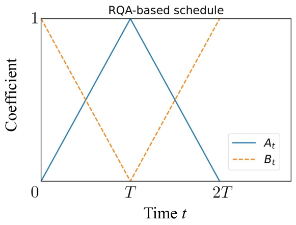
(a)

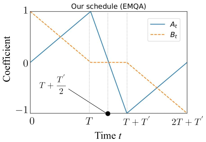
(b)

Figure 4: Two schedules of QA to implement the EM method called dual-state purification. (a) A schedule inspired by RQA. The dynamics from $t=0$ to $t=T$ ($t=T$ to $t=2T$) corresponds to the noisy map $\mathcal{F}$ ($\mathcal{G}$) in Eq. (2). At $t=T$, we perform a projective measurement to calculate the numerator in Eq. (4). In Sec. V, we show that we cannot accurately estimate the ground-state energy of $H_{\mathrm{P}}$ with this schedule. (b) An improved schedule tailored for the EM method. The dynamics from $t=0$ to $t=T+T^{{}^{\prime}}/2$ corresponds to the noisy map $\mathcal{F}$, and this schedule from $t=T+T^{{}^{\prime}}/2$ to $t=2T+T^{{}^{\prime}}$ provides a dynamics corresponding to the inverse map $\mathcal{G}$ in Eq. (2). For calculating the numerator in Eq. (4), a projective measurement is needed at $t=T+T^{{}^{\prime}}/2$.

To take into account decoherence, we adopt the Gorini–Kossakowski–Sudarshan–Lindblad (GKSL) master equation to describe the dynamics of the system

$$\dfrac{d\rho}{dt}=-i[H(t),\rho]+\sum_{n}\dfrac{\lambda_{n}}{2}\left(2\hat{L}_{n}\rho\hat{L}^{\dagger}_{n}-\left\{\hat{L}_{n}^{\dagger}\hat{L}_{n},\rho\right\}\right),$$ (12)

where $[\bullet,\bullet]$ denotes the commutator, $\lambda_{n}$ denotes a decay rate, $\hat{L}_{n}$ denotes the Lindblad operator, and $\{\bullet,\bullet\}$ denotes the anticommutator.

Throughout this paper, we assume that we can realize both the dynamics induced by the Hamiltonian and arbitrary single-qubit operations. Due to the recent development of quantum technologies, such a device is feasible, which we will discuss later. However, it is unclear whether we can implement two-qubit gates with high fidelity, and so we assume that we cannot perform two-qubit gates on the devices. This assumption is similar to that of digital-analog quantum computation (DAQC) Parra-Rodriguez et al. (2020). This approach has been proposed as a hybrid architecture to realize the flexibility of NISQ computation on robust analog quantum simulators.

It is worth mentioning that dual-state purification is more suitable for the device considered by us than virtual distillation. Although virtual distillation is also an efficient method to suppress stochastic errors, virtual distillation requires two-qubit gates to entangle $M$ copies of a noisy state $\rho$. Thus, it is not straightforward to implement virtual distillation under our assumption. On the other hand, in dual-state purification, we do not need to prepare $M$ copies of a noisy state $\rho$ or implement two-qubit gates as we mentioned in the previous section. This means that EMQA is more practical to mitigate noise effects during QA.

V Results

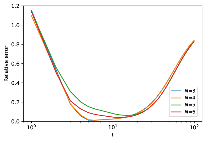
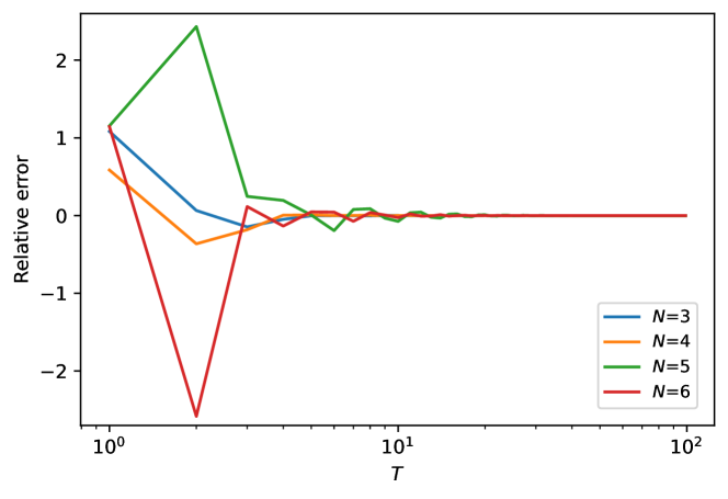
(a) EMQA schedule $\lambda=0$	(b) EMQA schedule $\lambda=0.004$
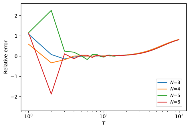
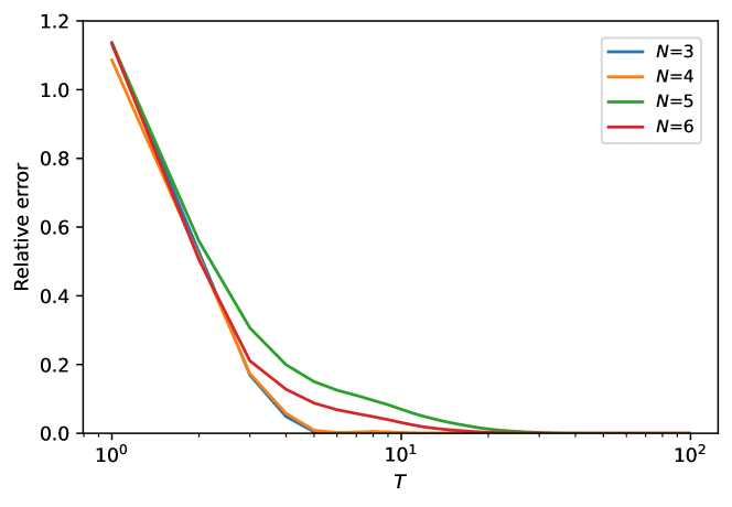
(c) RQA-based schedule $\lambda=0$	(d) RQA-based schedule $\lambda=0.004$
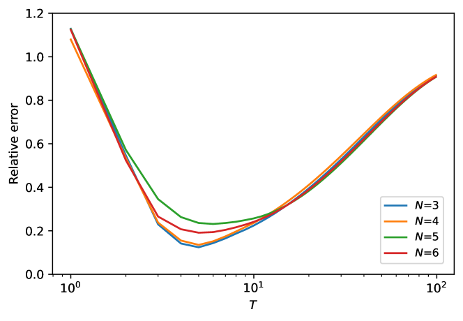
(e) Conventional schedule $\lambda=0$	(f) Conventional schedule $\lambda=0.004$

Figure 5: A relative error of the ground-state energy of the problem Hamiltonian $H_{\mathrm{P}}$. We define the relative error as $(\expectationvalue{H_{\mathrm{P}}}-E_{\mathrm{g}})/\absolutevalue{E_{\mathrm{g}}}$ where $\expectationvalue{H_{\mathrm{P}}}$ denotes the expectation value with QA and $E_{\mathrm{g}}$ denotes the actual value of the ground-state energy. We use (a) the EMQA, (c) RQA-based, and (e) conventional schedules with $\lambda=0$, while we adopt (b) the EMQA, (d) RQA-based, and (f) conventional schedules with $\lambda/J=0.004$. The annealing time $T$ is normalized by $J$. We show that the EMQA schedule provides the minimum error lower than that of the conventional method for all $N$ (see Table 1). Also, we show that the relative error with the RQA-based schedule can be lower than zero in some $T$ for all $N$. This means that the RQA-based schedule may produce unphysical results where a corresponding density matrix has negative eigenvalues.

In this section, we show the performance of the EMQA schedule and compare it with that of the RQA-based and the conventional schedules. For this purpose, we consider the problem Hamiltonian as the Heisenberg model described by

$$H_{\mathrm{P}}=J\sum^{N}_{i=1}(\hat{\sigma}^{x}_{i}\hat{\sigma}^{x}_{i+1}+\hat{\sigma}^{y}_{i}\hat{\sigma}^{y}_{i+1}+\Delta\hat{\sigma}^{z}_{i}\hat{\sigma}^{z}_{i+1}),$$ (13)

with the periodic boundary condition where $J$ and $\Delta$ are coefficients. Throughout of this paper, by setting $J=1$, the time and energy are normalized by this value. To simplify the discussion, we choose the Lindblad operators as the Pauli matrices $\hat{\sigma}_{i}^{x},\hat{\sigma}_{i}^{y}$, and $\hat{\sigma}_{i}^{z}$ and assume that the decay rate is constant regardless of the index (i.e. $\lambda_{n}=\lambda$). In our numerical simulation, the GKSL master equation is rewritten by

$$\dfrac{d\rho}{dt}=-i[H(t),\rho]-\dfrac{\lambda}{2}\sum_{i=1}^{N}\sum_{j\in\{x,y,z\}}[\hat{\sigma}_{i}^{j},[\hat{\sigma}_{i}^{j},\rho]].$$ (14)

Also, we set $B/J=1$, $T^{{}^{\prime}}J=5$, and $\Delta=-1$. To evaluate the performances of those schedules, we define a relative error as $(\expectationvalue{H_{\mathrm{P}}}-E_{\mathrm{g}})/\absolutevalue{E_{\mathrm{g}}}$ where $\expectationvalue{H_{\mathrm{P}}}$ is the expectation value of the problem Hamiltonian obtained with the numerical simulations and $E_{\mathrm{g}}$ denotes the ground-state energy of the problem Hamiltonian.

We plot the relative error against the parameter $T$ by changing the number of qubits in Fig. 5. We observe that there is an optimal $T$ to minimize the expectation values. This is because, as we increase $T$, the decoherence becomes more relevant while non-adiabatic transitions become less significant. Also, we indicate the minimum values of the expectation values and the relative errors with the numerical simulations in Table 1.

Table 1: The minimum value of the expectation value $\expectationvalue{H_{\mathrm{P}}}$ (and the relative error) obtained by each schedule with $\lambda=0.004$ and the exact value of the ground-state energy.

Expectation Value (Relative Error) $\lambda=0.004$
	EMQA	RQA-based	Conventional	Exact
$N=3$	$-2.96\ (0.0119)$	$-3.41\ (-0.138)$	$-2.63\ (0.124)$	$-3.00$
$N=4$	$-3.95\ (0.0114)$	$-5.32\ (-0.329)$	$-3.46\ (0.135)$	$-4.00$
$N=5$	$-4.69\ (0.0624)$	$-5.83\ (-0.167)$	$-3.84\ (0.231)$	$-5.00$
$N=6$	$-5.76\ (0.0395)$	$-17.2\ (-1.87)$	$-4.85\ (0.191)$	$-6.00$

In Fig. 5 we show the result of the numerical simulation with the EMQA schedule with $\lambda=0$. We check that the relative errors converge to zero regardless of the number of qubits when there is no decoherence. In addition, we show that even under the effect of the decoherence with $\lambda/J=0.004$, we can obtain a more accurate estimation of the ground-state energy than the conventional method, as shown in Table 1.

On the other hand, in Fig. 5 and 5, we show the performance of the method with the RQA-based schedule. Regardless of the number of qubits, the minimum expectation values are lower than the ground energies as shown in Table 1. If we calculate the energy by using ${\rm{Tr}}[\rho H_{\mathrm{P}}]$, we always have ${\rm{Tr}}[\rho H_{\mathrm{P}}]\geq E_{\mathrm{g}}$ where $\rho$ denotes an arbitrary density matrix. This means that the method with the RQA-based schedule provides us with an unphysical state. In this case, even if we minimize the expectation value of the energy by changing $T$, the minimized value is not always the closest to the actual value. This is a significant disadvantage to use the method with the RQA-based schedule.

Finally, let us discuss the physical implementation of our scheme. It is known that we can use superconducting flux qubits (or capacitively shunted flux qubits) for both QA and gate-type quantum computation Matsuzaki et al. (2020). Also, the Hamiltonian of the Heisenberg model with transverse fields can be realized by using these systems Imoto et al. (2022). For these systems, the coherence time can be as long as tens of micro seconds Yan et al. (2016), and the coupling strength can be tens of MHz or more Plantenberg et al. (2007). This means that, by using these quantum devices, we can realize $J/\lambda\simeq 10^{3}$, which is similar to those used in our simulations. Therefore, these systems are candidates for realizing our proposal.

VI Conclusion

In conclusion, we propose a QA strategy combined with an EM method to suppress the effects of decoherence. Among many EM methods, we adopt dual-state purification that does not require any two-qubit gates, which is suitable for the devices devised for QA. There are four steps in our protocol. First, let the system evolve by the Hamiltonian. Second, we perform single-qubit projective measurements. Third, let the system evolve by the Hamiltonian whose dynamics corresponds to an inverse map of the first dynamics. Finally, we post-process the measurement results. We numerically show that, by using our protocol, we can estimate the ground-state energy more accurately than the conventional QA under decoherence.

Appendix A Proof for inverse map in EMQA schedule

For dual-state purification, we need to construct an inverse transformation of the target unitary dynamics. Here, we show that, with the EMQA schedule, the dynamics from $t=T+T^{{}^{\prime}}/2$ to $t=2T+T^{{}^{\prime}}$ is equivalent to the conjugate transpose of the dynamics from $t=0$ to $t=T+T^{{}^{\prime}}/2$ when there is no decoherence.

First, the dynamics from $t=T+T^{{}^{\prime}}/2$ to $t=T+T^{{}^{\prime}}$ is equivalent to the conjugate transpose of the dynamics from $t=T$ to $t=T+T^{{}^{\prime}}/2$, i.e.,

$$\exp(-i\int_{T+T^{{}^{\prime}}/2}^{T+T^{{}^{\prime}}}A_{t}H_{\mathrm{P}}dt)=\exp(iH_{\mathrm{P}}\dfrac{T^{{}^{\prime}}}{4})$$ (15)

$$= \exp(-i\int_{T}^{T+T^{{}^{\prime}}/2}A_{t}H_{\mathrm{P}}dt)^{{\dagger}}$$

Next, let us consider the dynamics from $t=T+T^{{}^{\prime}}$ to $t=2T+T^{{}^{\prime}}$. By transforming the variable $t\ (t:T+T^{{}^{\prime}}\rightarrow 2T+T^{{}^{\prime}})$ into a variable $s\ (s:0\rightarrow T)$ by $t=s+T+T^{{}^{\prime}}$, we obtain

$$H_{2}(s)=\left(\dfrac{s}{T}-1\right)H_{\mathrm{P}}-\dfrac{s}{T}H_{\mathrm{D}}.$$ (16)

Thus, by using the Trotter decomposition, the dynamics of the Hamiltonian $H_{2}(s)$ is written as follows:

$$\mathcal{T}\exp(-i\int_{0}^{T}H_{2}(s)ds)$$ (17)

$$\simeq \exp\Bigl(-iH_{2}(M\delta t)\delta t\Bigr{missing})\times\exp\Bigl(-iH_{2}\bigl{(}(M-1)\delta t\bigr{)}\delta t\Bigr{missing})\times\cdots$$

$$\times\exp\Bigl(-iH_{2}(\delta t)\delta t\Bigr{missing})\times\exp\Bigl(-iH_{2}(0)\delta t\Bigr{missing})$$

$$= \prod_{j=0}^{M}\exp\Bigl(-iH_{2}(j\delta t)\delta t\Bigr{missing}),$$

where $\mathcal{T}$ denotes the time-ordered product, $M$ denotes a natural number, and $\delta t=T/M$ denotes a discretized time. Note that $\mathcal{T}\exp(-i\int_{0}^{T}H_{2}(s)ds)$ is equal to the second line in the limit of a small $\delta t$. Meanwhile, We define the time-dependent Hamiltonian from $t=0$ to $t=T$ as

$$H_{1}(t)=\dfrac{t}{T}H_{\mathrm{P}}+\left(1-\dfrac{t}{T}\right)H_{\mathrm{D}}.$$ (18)

We can decompose the conjugate transpose of the dynamics from $t=0$ to $t=T$ as

$$\Biggl{(}\mathcal{T}\exp(-i\int_{0}^{T}H_{1}(t)dt)\Biggr{)}^{{\dagger}}$$ (19)

$$\simeq \Biggl{(}\exp\Bigl(-iH_{1}(M\delta t)\delta t\Bigr{missing})\times\exp\Bigl(-iH_{1}\Bigl{(}(M-1)\delta t\Bigr{)}\delta t\Bigr{missing})\times\cdots$$

$$\times\exp\Bigl(-iH_{1}(\delta t)\delta t\Bigr{missing})\times\exp\Bigl(-iH_{1}(0)\delta t\Bigr{missing})\Biggr{)}^{{\dagger}}$$

$$= \exp\Bigl(iH_{1}(0)\delta t\Bigr{missing})\times\exp\Bigl(iH_{1}(\delta t)\delta t\Bigr{missing})\times\cdots$$

$$\times\exp\Bigl(iH_{1}\Bigl{(}(M-1)\delta t\Bigr{)}\delta t\Bigr{missing})\times\exp\Bigl(iH_{1}(M\delta t)\delta t\Bigr{missing})$$

$$= \prod_{j=0}^{M}\exp\Bigl(iH_{1}\Bigl{(}(M-j)\delta t\Bigr{)}\delta t\Bigr{missing}).$$

Since $\exp\Bigl(-iH_{2}(j\delta t)\delta t\Bigr{missing})=\exp\Bigl(iH_{1}\bigl{(}(M-j)\delta t\bigr{)}\delta t\Bigr{missing})$ is satisfied in each index $j$, we have

$$\mathcal{T}\exp(-i\int_{0}^{T}H_{2}(s)ds)$$ (20)

$$= \lim_{M\to\infty}\prod_{j=0}^{M}\exp\Bigl(-iH_{2}(j\delta t)\delta t\Bigr{missing})=\lim_{M\to\infty}\prod_{j=0}^{M}\exp\Bigl(iH_{1}\bigl{(}(M-j)\delta t\bigr{)}\delta t\Bigr{missing})$$

$$= \Biggl{(}\mathcal{T}\exp(-i\int_{0}^{T}H_{1}(t)dt)\Biggr{)}^{{\dagger}}.$$

Therefore, by using Eq. 15 and 20, we show

$$\mathcal{T}\exp(-i\int_{T+T^{{}^{\prime}}/2}^{2T+T^{{}^{\prime}}}\Bigl{(}A_{t}H_{\mathrm{P}}+B_{t}H_{\mathrm{D}}\Bigr{)}dt)$$ (21)

$$= \mathcal{T}\exp(-i\int_{0}^{T}H_{2}(s)ds)\exp(-i\int_{T+T^{{}^{\prime}}/2}^{T+T^{{}^{\prime}}}A_{t}H_{\mathrm{P}}dt)$$

$$= \Biggl{(}\mathcal{T}\exp(-i\int_{0}^{T}H_{1}(t)dt)\Biggr{)}^{{\dagger}}\exp(-i\int_{T}^{T+T^{{}^{\prime}}/2}A_{t}H_{\mathrm{P}}dt)^{{\dagger}}$$

$$= \Biggl{(}\mathcal{T}\exp(-i\int_{0}^{T+T^{{}^{\prime}}/2}\Bigl{(}A_{t}H_{\mathrm{P}}+B_{t}H_{\mathrm{D}}\Bigr{)}dt)\Biggr{)}^{{\dagger}}.$$

Appendix B Theoretical analysis for RQA-based schedule

In the main text, we observe that the expectation value of $H_{\mathrm{P}}$ becomes lower than the ground energy with the RQA-based method in the numerical simulations. To obtain a better understanding of this, we derive analytic expressions of the RQA-based method with a single qubit. Actually, we will show that, for this case, the state $\rho\bar{\rho}+\bar{\rho}\rho$ becomes unphysical in the sense that the eigenvalues of this state become lower than 0 unlike physical density matrices. In this section, we do not consider the effect of decoherence since we can see such an unphysical situation even if there is no decoherence as shown in Fig. 5. We set a time-dependent Hamiltonian from $t=0$ to $t=T$ for the QA as

$$H(t)=-\sin\Biggl(\dfrac{\pi t}{2T}\Biggr{missing})\hat{\sigma}^{z}-\cos\Biggl(\dfrac{\pi t}{2T}\Biggr{missing})\hat{\sigma}^{x}.$$ (22)

We can diagonalize this Hamiltonian with a unitary matrix written as

$$V(t)=\begin{pmatrix}\cos(\dfrac{\pi(t+T)}{4T})&-\sin(\dfrac{\pi(t+T)}{4T})\\ \ &\ \\ \sin(\dfrac{\pi(t+T)}{4T})&\cos(\dfrac{\pi(t+T)}{4T})\\ \end{pmatrix}.$$ (23)

We obtain a diagonalized matrix as

$$D\equiv V(t)H(t)V^{{\dagger}}(t)=\begin{pmatrix}1&0\\ 0&-1\end{pmatrix}.$$ (24)

By using those matrices $V(t)$ and $D$, we define an effective Hamiltonian as

$$H_{\mathrm{eff}} = i\dfrac{dV(t)}{dt}V^{{\dagger}}(t)+D$$ (25)

$$= \begin{pmatrix}1&-\dfrac{i\pi}{4T}\\ \ &\ \\ \dfrac{i\pi}{4T}&-1\end{pmatrix}.$$

If there is no decoherence, the time-evolved state $\ket{\psi(T)}$ with the Hamiltonian $H(t)$ from the initial state $\ket{+}$ is written as

$$\ket{\psi(T)} = \mathcal{T}\exp(-i\int_{0}^{T}H(t)dt)\ket{+}$$ (29)

$$= V^{{\dagger}}(T)\exp(-iTH_{\mathrm{eff}})V(0)\ket{+}$$

$$= \left(\begin{array}[]{c}\cos\Biggl(\dfrac{1}{4}\sqrt{\pi^{2}+16T^{2}}\Biggr{missing})+\dfrac{4iT\sin\Biggl(\dfrac{1}{4}\sqrt{\pi^{2}+16T^{2}}\Biggr{missing})}{\sqrt{\pi^{2}+16T^{2}}}\\ \\ \dfrac{\pi\sin\Biggl(\dfrac{1}{4}\sqrt{\pi^{2}+16T^{2}}\Biggr{missing})}{\sqrt{\pi^{2}+16T^{2}}}\end{array}\right).$$

In this case, we obtain the density matrix $\rho$ as $\outerproduct*{\psi(T)}{\psi(T)}$.

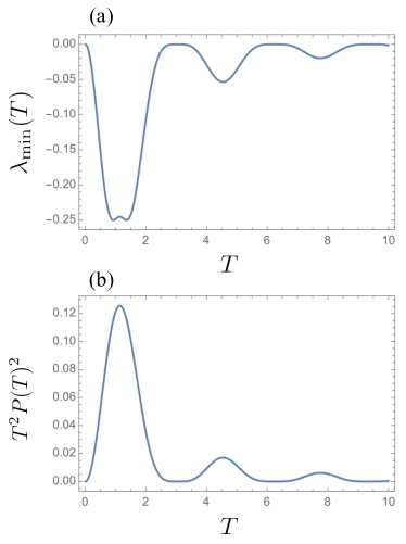
Figure 6: The relationship between the transition rate $P(T)$ in Eq. (41) and the minimum eigenvalue $\lambda_{\mathrm{min}}(T)$ in Eq. (39) of the state $\rho\bar{\rho}+\bar{\rho}\rho$. We plot $\lambda_{\mathrm{min}}(T)$ and $T^{2}P(T)^{2}$ against the annealing time $T$ in Fig. 6 (a) and (b), respectively. We check they have peaks at the same points of $T$. This is the evidence in which the eigenvalue is deeply connected with the non-adiabatic transition as shown by Eq. (42).

On the other hand, the time-dependent Hamiltonian from $t=T$ to $t=2T$ which corresponds to the inverse map $\mathcal{G}$ is defined as

$$H(t)=-\cos\Biggl(\dfrac{\pi}{2T}(t-T)\Biggr{missing})\hat{\sigma}^{z}-\sin\Biggl(\dfrac{\pi}{2T}(t-T)\Biggr{missing})\hat{\sigma}^{x}.$$ (31)

We can also diagonalize this Hamiltonian with a unitary matrix written as

$$U(t)=\begin{pmatrix}\sin(\dfrac{\pi(t-T)}{4T})&-\cos(\dfrac{\pi(t-T)}{4T})\\ \ &\ \\ \cos(\dfrac{\pi(t-T)}{4T})&\sin(\dfrac{\pi(t-T)}{4T})\\ \end{pmatrix}.$$ (32)

We obtain an effective Hamiltonian during this time range as

$$H_{\mathrm{eff}}^{{}^{\prime}} = i\dfrac{dU(t)}{dt}U(t)^{{\dagger}}+D$$ (33)

$$= \begin{pmatrix}1&\dfrac{i\pi}{4T}\\ \ &\ \\ -\dfrac{i\pi}{4T}&-1\end{pmatrix}$$

because the diagonalized matrix of the Hamiltonian in Eq. (31) is also $D$. By using this effective Hamiltonian, we define a state $\ket{\phi(T)}$ as

$$\ket{\phi(T)} = \Biggl{(}\mathcal{T}\exp(-i\int_{T}^{2T}H(t)dt)\Biggr{)}^{{\dagger}}\ket{+}$$ (37)

$$= \Biggl{(}U(2T)^{{\dagger}}\exp(-iTH_{\mathrm{eff}}^{{}^{\prime}})U(T)\Biggr{)}^{{\dagger}}\ket{+}$$

$$= \left(\begin{array}[]{c}\cos\Biggl(\dfrac{1}{4}\sqrt{\pi^{2}+16T^{2}}\Biggr{missing})-\dfrac{4iT\sin\Biggl(\dfrac{1}{4}\sqrt{\pi^{2}+16T^{2}}\Biggr{missing})}{\sqrt{\pi^{2}+16T^{2}}}\\ \\ \dfrac{\pi\sin\Biggl(\dfrac{1}{4}\sqrt{\pi^{2}+16T^{2}}\Biggr{missing})}{\sqrt{\pi^{2}+16T^{2}}}\end{array}\right).$$

By using this state, we have $\bar{\rho}$ in Eq. 2 as $\outerproduct*{\phi(T)}{\phi(T)}$. For our purpose, it is sufficient to consider only $\rho\bar{\rho}+\bar{\rho}\rho$ because $\Tr[\rho\bar{\rho}+\bar{\rho}\rho\Bigr{]}>0$ is satisfied in this case. We obtain the minimum eigenvalue $\lambda_{\mathrm{min}}(T)$ of the state $\rho\bar{\rho}+\bar{\rho}\rho$ as

$$\lambda_{\mathrm{min}}(T)=\dfrac{A-(\pi^{2}+16T^{2})\sqrt{A}}{(\pi^{2}+16T^{2})^{2}},$$ (39)

where

$$A= \pi^{4}+8\pi^{2}T^{2}+256T^{4}+32\pi^{2}T^{2}\cos\Biggl(\dfrac{1}{2}\sqrt{\pi^{2}+16T^{2}}\Biggr{missing})$$ (40)

$$-8\pi^{2}T^{2}\cos\Biggl(\sqrt{\pi^{2}+16T^{2}}\Biggr{missing}).$$

We plot $\lambda_{\mathrm{min}}(T)$ against the parameter $T$ in Fig. 6 (a). As we can see in Fig. 6 (a), $\lambda_{\mathrm{min}}(T)$ can be negative for some $T$. Thus, the state $\rho\bar{\rho}+\bar{\rho}\rho$ is unphysical in the sense that the eigenvalue is negative even if we normalize this state. As long as the state $\rho\bar{\rho}+\bar{\rho}\rho$ has a negative eigenvalue, the expectation values of the energy $\Tr[H_{\mathrm{P}}(\rho\bar{\rho}+\bar{\rho}\rho)\Bigr{]}/\Tr[\rho\bar{\rho}+\bar{\rho}\rho\Bigr{]}$ can be lower than the ground-state energy.

We expect that this negative eigenvalue of $\rho\bar{\rho}+\bar{\rho}\rho$ is related to the non-adiabatic transitions during QA. Actually, we confirm that the unphysical state appears at relatively small $T$ as shown in Fig. 5. For further investigation, we define a transition rate $P(T)$ as

$$P(T)=|\innerproduct{1}{\psi(T)}|^{2}=\dfrac{\pi^{2}\sin^{2}\Biggl{(}\dfrac{\sqrt{\pi^{2}+16T^{2}}}{4}\Biggr{)}}{\pi^{2}+16T^{2}}.$$ (41)

When $P(T)$ is not zero, there are non-adiabatic transitions during the dynamics. By using the transition rate $P(T)$, we rewrite

$$\lambda_{\mathrm{min}}(T)=\Biggl{(}\sqrt{1-\dfrac{64T^{2}P(T)^{2}}{\pi^{2}}}-\dfrac{1}{2}\Biggr{)}^{2}-\dfrac{1}{4}.$$ (42)

We plot $T^{2}P(T)^{2}$ against the parameter $T$ in Fig. 6 (b). We confirm that the eigenvalue $\lambda_{\mathrm{min}}(T)$ decreases (increases) as $T^{2}P(T)^{2}$ increases (decreases) in Fig. 6. This shows that the non-adiabatic transitions are deeply related to the negative eigenvalues of the state $\rho\bar{\rho}+\bar{\rho}\rho$ in Eq. (42).

References

- Kadowaki and Nishimori (1998) T. Kadowaki and H. Nishimori, Physical Review E 58, 5355 (1998).
- Farhi et al. (2000) E. Farhi, J. Goldstone, S. Gutmann, and M. Sipser, arXiv preprint quant-ph/0001106 (2000).
- Farhi et al. (2001) E. Farhi, J. Goldstone, S. Gutmann, J. Lapan, A. Lundgren, and D. Preda, Science 292, 472 (2001).
- Ehrenfest (1916) P. Ehrenfest, Adiabatische Invarianten und Quantentheorie, Vol. 356 (Annalen der Physik, 1916).
- Kato (1950) T. Kato, Journal of the Physical Society of Japan 5, 435 (1950).
- Amin (2009) M. H. Amin, Physical Review Letters 102, 220401 (2009).
- Dodin and Brumer (2021) A. Dodin and P. Brumer, PRX Quantum 2, 030302 (2021).
- Lechner et al. (2015) W. Lechner, P. Hauke, and P. Zoller, Science Advances 1, e1500838 (2015).
- Kumar et al. (2018) V. Kumar, G. Bass, C. Tomlin, and J. Dulny, Quantum Information Processing 17, 1 (2018).
- Choi (2011) V. Choi, Quantum Information Processing 10, 343 (2011).
- Morita and Nishimori (2008) S. Morita and H. Nishimori, Journal of Mathematical Physics 49, 125210 (2008).
- Albert (1961) M. Albert, Quantum mechanics, Vol. 1 (John Wiley & Sons Incorporated, 1961).
- Albert (1962) M. Albert, Quantum mechanics, Vol. II (North-Holland Publishing Company, 1962).
- Roland and Cerf (2005) J. Roland and N. J. Cerf, Physical Review A 71, 032330 (2005).
- Åberg et al. (2005) J. Åberg, D. Kult, and E. Sjöqvist, Physical Review A 72, 042317 (2005).
- Albash and Lidar (2015) T. Albash and D. A. Lidar, Physical Review A 91, 062320 (2015).
- Childs et al. (2001) A. M. Childs, E. Farhi, and J. Preskill, Physical Review A 65, 012322 (2001).
- Sarandy and Lidar (2005) M. Sarandy and D. Lidar, Physical Review Letters 95, 250503 (2005).
- Preskill (2018) J. Preskill, Quantum 2, 79 (2018).
- Endo et al. (2021) S. Endo, Z. Cai, S. C. Benjamin, and X. Yuan, Journal of the Physical Society of Japan 90, 032001 (2021).
- Cerezo et al. (2021) M. Cerezo, A. Arrasmith, R. Babbush, S. C. Benjamin, S. Endo, K. Fujii, J. R. McClean, K. Mitarai, X. Yuan, L. Cincio, et al., Nature Reviews Physics 3, 625 (2021).
- Peruzzo et al. (2014) A. Peruzzo, J. McClean, P. Shadbolt, M.-H. Yung, X.-Q. Zhou, P. J. Love, A. Aspuru-Guzik, and J. L. O’brien, Nature Communications 5, 1 (2014).
- Li and Benjamin (2017) Y. Li and S. C. Benjamin, Physical Review X 7, 021050 (2017).
- McClean et al. (2016) J. R. McClean, J. Romero, R. Babbush, and A. Aspuru-Guzik, New Journal of Physics 18, 023023 (2016).
- Yuan et al. (2019) X. Yuan, S. Endo, Q. Zhao, Y. Li, and S. C. Benjamin, Quantum 3, 191 (2019).
- Endo et al. (2020) S. Endo, J. Sun, Y. Li, S. C. Benjamin, and X. Yuan, Phys. Rev. Lett. 125, 010501 (2020).
- Kandala et al. (2019) A. Kandala, K. Temme, A. D. Córcoles, A. Mezzacapo, J. M. Chow, and J. M. Gambetta, Nature 567, 491 (2019).
- Temme et al. (2017) K. Temme, S. Bravyi, and J. M. Gambetta, Physical Review Letters 119, 180509 (2017).
- Endo et al. (2018) S. Endo, S. C. Benjamin, and Y. Li, Physical Review X 8, 031027 (2018).
- Song et al. (2019) C. Song, J. Cui, H. Wang, J. Hao, H. Feng, and Y. Li, Science Advances 5, eaaw5686 (2019).
- Zhang et al. (2020) S. Zhang, Y. Lu, K. Zhang, W. Chen, Y. Li, J.-N. Zhang, and K. Kim, Nature Communications 11, 1 (2020).
- McArdle et al. (2019) S. McArdle, X. Yuan, and S. Benjamin, Physical Review Letters 122, 180501 (2019).
- Bonet-Monroig et al. (2018) X. Bonet-Monroig, R. Sagastizabal, M. Singh, and T. O’Brien, Physical Review A 98, 062339 (2018).
- Sun et al. (2021) J. Sun, X. Yuan, T. Tsunoda, V. Vedral, S. C. Benjamin, and S. Endo, Physical Review Applied 15, 034026 (2021).
- LaRose et al. (2022) R. LaRose, A. Mari, S. Kaiser, P. J. Karalekas, A. A. Alves, P. Czarnik, M. El Mandouh, M. H. Gordon, Y. Hindy, A. Robertson, et al., Quantum 6, 774 (2022).
- Quantum et al. (2020) G. A. Quantum, Collaborators*†, F. Arute, K. Arya, R. Babbush, D. Bacon, J. C. Bardin, R. Barends, S. Boixo, M. Broughton, B. B. Buckley, et al., Science 369, 1084 (2020).
- McClean et al. (2017) J. R. McClean, M. E. Kimchi-Schwartz, J. Carter, and W. A. De Jong, Physical Review A 95, 042308 (2017).
- Merkel et al. (2013) S. T. Merkel, J. M. Gambetta, J. A. Smolin, S. Poletto, A. D. Córcoles, B. R. Johnson, C. A. Ryan, and M. Steffen, Physical Review A 87, 062119 (2013).
- Stark (2014) C. Stark, Physical Review A 89, 052109 (2014).
- Greenbaum (2015) D. Greenbaum, arXiv preprint arXiv:1509.02921 (2015).
- Blume-Kohout et al. (2017) R. Blume-Kohout, J. K. Gamble, E. Nielsen, K. Rudinger, J. Mizrahi, K. Fortier, and P. Maunz, Nature Communications 8, 1 (2017).
- Strikis et al. (2021) A. Strikis, D. Qin, Y. Chen, S. C. Benjamin, and Y. Li, PRX Quantum 2, 040330 (2021).
- Czarnik et al. (2021a) P. Czarnik, A. Arrasmith, P. J. Coles, and L. Cincio, Quantum 5, 592 (2021a).
- Wang et al. (2021) Z. Wang, Y. Chen, Z. Song, D. Qin, H. Li, Q. Guo, H. Wang, C. Song, and Y. Li, Physical Review Letters 126, 080501 (2021).
- O’Brien et al. (2021) T. E. O’Brien, S. Polla, N. C. Rubin, W. J. Huggins, S. McArdle, S. Boixo, J. R. McClean, and R. Babbush, PRX Quantum 2, 020317 (2021).
- Yoshioka et al. (2022) N. Yoshioka, H. Hakoshima, Y. Matsuzaki, Y. Tokunaga, Y. Suzuki, and S. Endo, Physical Review Letters 129, 020502 (2022).
- Cai et al. (2022) Z. Cai, R. Babbush, S. C. Benjamin, S. Endo, W. J. Huggins, Y. Li, J. R. McClean, and T. E. O’Brien, arXiv preprint arXiv:2210.00921 (2022).
- Cao et al. (2022) C. Cao, Y. Yu, Z. Wu, N. Shannon, B. Zeng, and R. Joynt, Quantum Science and Technology (2022).
- Huo and Li (2021) M. Huo and Y. Li, Communications in Theoretical Physics 73, 075101 (2021).
- Takagi (2021) R. Takagi, Physical Review Research 3, 033178 (2021).
- Hakoshima et al. (2021) H. Hakoshima, Y. Matsuzaki, and S. Endo, Physical Review A 103, 012611 (2021).
- Suzuki et al. (2022) Y. Suzuki, S. Endo, K. Fujii, and Y. Tokunaga, PRX Quantum 3, 010345 (2022).
- Koczor (2021) B. Koczor, Physical Review X 11, 031057 (2021).
- Huggins et al. (2021) W. J. Huggins, S. McArdle, T. E. O’Brien, J. Lee, N. C. Rubin, S. Boixo, K. B. Whaley, R. Babbush, and J. R. McClean, Physical Review X 11, 041036 (2021).
- Czarnik et al. (2021b) P. Czarnik, A. Arrasmith, L. Cincio, and P. J. Coles, arXiv preprint arXiv:2102.06056 (2021b).
- Yamamoto et al. (2021) K. Yamamoto, S. Endo, H. Hakoshima, Y. Matsuzaki, and Y. Tokunaga, arXiv preprint arXiv:2112.01850 (2021).
- Huo and Li (2022) M. Huo and Y. Li, Physical Review A 105, 022427 (2022).
- Susa et al. (2018a) Y. Susa, Y. Yamashiro, M. Yamamoto, and H. Nishimori, Journal of the Physical Society of Japan 87, 023002 (2018a).
- Susa et al. (2018b) Y. Susa, Y. Yamashiro, M. Yamamoto, I. Hen, D. A. Lidar, and H. Nishimori, Physical Review A 98, 042326 (2018b).
- Seki and Nishimori (2012) Y. Seki and H. Nishimori, Physical Review E 85, 051112 (2012).
- Seki and Nishimori (2015) Y. Seki and H. Nishimori, Journal of Physics A: Mathematical and Theoretical 48, 335301 (2015).
- Matsuzaki et al. (2021) Y. Matsuzaki, H. Hakoshima, K. Sugisaki, Y. Seki, and S. Kawabata, Japanese Journal of Applied Physics 60, SBBI02 (2021).
- Mori et al. (2022) Y. Mori, S. Kawabata, and Y. Matsuzaki, arXiv preprint arXiv:2208.02553 (2022).
- Pudenz et al. (2014) K. L. Pudenz, T. Albash, and D. A. Lidar, Nature Communications 5, 1 (2014).
- Suzuki and Nakazato (2020) T. Suzuki and H. Nakazato, arXiv preprint arXiv:2006.13440 (2020).
- Chen et al. (2011) H. Chen, X. Kong, B. Chong, G. Qin, X. Zhou, X. Peng, and J. Du, Physical Review A 83, 032314 (2011).
- Nakahara (2013) M. Nakahara, Lectures on quantum computing, thermodynamics and statistical physics, Vol. 8 (World Scientific, 2013).
- Matsuzaki et al. (2020) Y. Matsuzaki, H. Hakoshima, Y. Seki, and S. Kawabata, Japanese Journal of Applied Physics 59, SGGI06 (2020).
- Crosson et al. (2014) E. Crosson, E. Farhi, C. Y.-Y. Lin, H.-H. Lin, and P. Shor, arXiv preprint arXiv:1401.7320 (2014).
- Goto and Kanao (2020) H. Goto and T. Kanao, arXiv preprint arXiv:2005.07511 (2020).
- Hormozi et al. (2017) L. Hormozi, E. W. Brown, G. Carleo, and M. Troyer, Physical Review B 95, 184416 (2017).
- Muthukrishnan et al. (2016) S. Muthukrishnan, T. Albash, and D. A. Lidar, Physical Review X 6, 031010 (2016).
- Brady and van Dam (2017) L. T. Brady and W. van Dam, Physical Review A 95, 032335 (2017).
- Somma et al. (2012) R. D. Somma, D. Nagaj, and M. Kieferová, Physical Review Letters 109, 050501 (2012).
- Das and Chakrabarti (2008) A. Das and B. K. Chakrabarti, Reviews of Modern Physics 80, 1061 (2008).
- Karanikolas and Kawabata (2020) V. Karanikolas and S. Kawabata, Journal of the Physical Society of Japan 89, 094003 (2020).
- Watabe et al. (2020) S. Watabe, Y. Seki, and S. Kawabata, Scientific Reports 10, 1 (2020).
- Susa and Nishimori (2021) Y. Susa and H. Nishimori, Physical Review A 103, 022619 (2021).
- Matsuura et al. (2021) S. Matsuura, S. Buck, V. Senicourt, and A. Zaribafiyan, Physical Review A 103, 052435 (2021).
- Passarelli et al. (2021) G. Passarelli, R. Fazio, and P. Lucignano, arXiv preprint arXiv:2109.13043 (2021).
- Imoto et al. (2021) T. Imoto, Y. Seki, Y. Matsuzaki, and S. Kawabata, arXiv preprint arXiv:2111.15283 (2021).
- Parra-Rodriguez et al. (2020) A. Parra-Rodriguez, P. Lougovski, L. Lamata, E. Solano, and M. Sanz, Physical Review A 101, 022305 (2020).
- Imoto et al. (2022) T. Imoto, Y. Seki, and Y. Matsuzaki, Journal of the Physical Society of Japan 91, 064004 (2022).
- Yan et al. (2016) F. Yan, S. Gustavsson, A. Kamal, J. Birenbaum, A. P. Sears, D. Hover, T. J. Gudmundsen, D. Rosenberg, G. Samach, S. Weber, et al., Nature Communications 7, 1 (2016).
- Plantenberg et al. (2007) J. Plantenberg, P. De Groot, C. Harmans, and J. Mooij, Nature 447, 836 (2007).
- Johansson et al. (2012) J. R. Johansson, P. D. Nation, and F. Nori, Computer Physics Communications 183, 1760 (2012).