Inexpensive polynomial-degree-robust
equilibrated flux a posteriori estimates
for isogeometric analysis

Abstract.

We consider isogeometric discretizations of the Poisson model problem, focusing on high polynomial degrees and strong hierarchical refinements. We derive a posteriori error estimates by equilibrated fluxes, i.e., vector-valued mapped piecewise polynomials lying in the $\bm{H}(\mathrm{div})$ space which appropriately approximate the desired divergence constraint. Our estimates are constant-free in the leading term, locally efficient, and robust with respect to the polynomial degree. They are also robust with respect to the number of hanging nodes arising in adaptive mesh refinement employing hierarchical B-splines. Two partitions of unity are designed, one with larger supports corresponding to the mapped splines, and one with small supports corresponding to mapped piecewise multilinear finite element hat basis functions. The equilibration is only performed on the small supports, avoiding the higher computational price of equilibration on the large supports or even the solution of a global system. Thus, the derived estimates are also as inexpensive as possible. An abstract framework for such a setting is developed, whose application to a specific situation only requests a verification of a few clearly identified assumptions. Numerical experiments illustrate the theoretical developments.

1. Introduction

A posteriori error estimates for standard finite element methods (FEM) are nowadays well understood [AO00, Rep08, Ver13]. On the one hand, they allow to assess the quality of the computed approximation, and, on the other hand, they indicate where to refine the underlying mesh of the computational domain. Among the existing error estimators, those based on equilibrated fluxes [PS47, LL83, DM99, BS08] have the advantage that they provide a guaranteed upper bound for the approximation error which is constant-free in the leading term. The estimator from [DM99, BS08] even turns out to be robust with respect to the polynomial degree [BPS09], i.e., it provides also a lower bound with an efficiency constant that does not depend on the polynomial degree. This result has been recently generalized in several directions; see [EV15, EV20] and the references therein. We also mention [DEV16], which covers standard FEM on triangular/rectangular meshes with hanging nodes, and its generalization to arbitrarily many hanging nodes [ESV17a].

In this work, we aim to generalize this result to isogeometric analysis (IGA) [HCB05, BBdVC⁺06, CHB09]. The central idea of IGA is to use the same ansatz functions for the representation of the problem geometry in computer-aided design (CAD) and for the discretization of the partial differential equation (PDE). While the CAD standard for spline representation in a multivariate setting relies on tensor-product B-splines, several extensions of the B-spline model have emerged that allow for adaptive refinement, e.g., hierarchical splines [VGJS11, GJS12], (analysis-suitable) T-splines [SZBN03, SLSH12, BdVBSV13], or LR-splines [DLP13, JKD14]; see also [JRK15, HKMP17, BGG⁺22] for a comparison of these approaches.

1.1. Available results

To steer an adaptive refinement, rigorous a posteriori error estimators have been developed. Assuming a certain admissibility condition of the employed meshes, the works [BG16b, GP20] generalize the weighted residual error estimator from standard FEM to IGA with hierarchical splines and analysis-suitable T-splines, respectively. It has even been proved that the corresponding adaptive algorithms converge at optimal algebraic rate with respect to the number of mesh elements [BG17, GHP17, GP20], see also the recent overview article [BGG⁺22]. However, the reliability and efficiency constants depend on the employed polynomial degree, which is indeed witnessed in numerical experiments, see, e.g., [BGG⁺22] for hierarchical splines. Similarly, for the hierarchical spline space from [BG16a], the work [BG18] derives a weighted residual estimator being the sum of indicators associated to basis functions instead of elements. It is shown to be reliable for arbitrary hierarchical meshes, with an unknown reliability constant that again particularly depends on the used polynomial degree $p$.

In the spirit of [Rep99, Rep00a, Rep00b], the works [KT15a, KT15b, Mat18] present guaranteed fully computable upper bounds of the approximation error for tensor-product splines and hierarchical splines, respectively. A second estimate is also derived, giving a lower bound of the error. However, to compute these so-called functional-type estimators, a global minimization problem may need to be solved or an $\bm{H}(\mathrm{div})$ flux not in the equilibrium with the load may be employed, and the efficiency of the upper bound, as well as the reliability of the lower bound, are theoretically unclear. In the recent work [TCHM19], a non-$\bm{H}(\mathrm{div})$ approximation of an equilibrated flux is constructed for tensor-product splines in extension of the concepts of [LL83]. It only requires to solve locally, on the knot spans, a pair of a low-order problem for the normal fluxes together with a high-order problem for the equilibrated flux approximation. A generalization to hierarchical splines is briefly sketched and a corresponding numerical example is provided. While this yields a fully computable and approximately guaranteed upper bound on the error, efficiency of the resulting estimator is unclear.

1.2. Outline

The present manuscript is organized as follows. We introduce the model problem and its general Galerkin discretization in Section 2. We then motivate and introduce our new approach in the simplified spline setting in Section 3. Sections 4 and 5 subsequently contain a detailed description of the discretization space formed by hierarchical B-splines. This technical description might be skipped in a first reading, since all our results are only based on a couple of abstract assumptions collected in Section 6, where we also verify them in the hierarchical B-splines setting. Section 7 describes in detail our inexpensive flux equilibration in the general context. The a posteriori error estimates are then derived in Section 8, where we prove their reliability and (local) efficiency. Numerical experiments illustrating the theoretical findings are collected in Section 9. Finally, Appendix A proves the broken polynomial extension property that is central for the polynomial-degree robustness in the present setting.

2. Model problem and its Galerkin discretization

Let $\Omega$ be an open bounded connected Lipschitz domain in $\mathbb{R}^{d}$ with $d=2,3$. We consider the Poisson model problem with homogeneous Dirichlet data of finding $u:\Omega\rightarrow\mathbb{R}$ such that

$$\begin{split}-\Delta u&=f\quad\text{in }\Omega,\\ u&=0\quad\text{on }\partial\Omega,\end{split}$$ (1)

where $f\in L^{2}(\Omega)$ is a given source term. On an arbitrary subset $\omega\subseteq\overline{\Omega}$, let $(\cdot\,,\,\cdot)_{\omega}:=\int_{\omega}(\cdot)(\cdot)\,{\rm d}x$ and $\|\cdot\|_{\omega}$ denote the $L^{2}$-scalar product and the corresponding norm, respectively; we also denote by $\|\cdot\|_{\infty,\omega}$ the $L^{\infty}$-norm. Then, the weak formulation of problem (1) consists in finding $u\in H_{0}^{1}(\Omega)$ such that

$$(\nabla u\,,\,\nabla v)_{\Omega}=(f\,,\,v)_{\Omega}\quad\text{for all }v\in H_{0}^{1}(\Omega).$$ (2)

Let $V_{h}$ be a finite-dimensional subspace of $H_{0}^{1}(\Omega)$. The corresponding Galerkin approximation is to find $u_{h}\in V_{h}$ with

$$(\nabla u_{h}\,,\,\nabla v_{h})_{\Omega}=(f\,,\,v_{h})_{\Omega}\quad\text{for all }v_{h}\in V_{h}.$$ (3)

In this work, we will choose $V_{h}$ as the space of mapped hierarchical splines. To this end, we assume that $\Omega$ can be parametrized over $\widehat{\Omega}:=(0,1)^{d}$ via a bi-Lipschitz mapping $\bm{F}:\widehat{\Omega}\to\Omega$ with positive Jacobian determinant, i.e., $\Omega$ = $\bm{F}(\widehat{\Omega})$, $\bm{F}\in W^{1,\infty}({\widehat{\Omega}})$, $\bm{F}^{-1}\in W^{1,\infty}(\Omega)$, and $\det(D\bm{F})>0$. Note that $\bm{F}$ and its inverse $\bm{F}^{-1}$ can both be continuously extended to Lipschitz continuous functions on $\overline{\widehat{\Omega}}$ and $\overline{\Omega}$, respectively.

3. Motivation and the new approach in a simplified spline setting

In this section, we recall equilibration for standard $C^{0}$ finite elements, discuss difficulties for a generalization to IGA, and introduce our new approach. In order to explain the main ideas as clearly as possible, we will consider a strongly simplified setting. In particular, we suppose in this section that $\bm{F}$ is just the identity, so that $\Omega=\widehat{\Omega}=(0,1)^{d}$, and that $\mathcal{T}_{h}$ is a uniform tensor-product mesh of $\Omega$ consisting of elements $K$ being all $d$-rectangular parallelepipeds. Let $\mathbb{Q}^{\bm{p}}(\mathcal{T}_{h})$ denote all $\mathcal{T}_{h}$-piecewise tensor-product polynomials of fixed degree $\bm{p}:=(p,\dots,p)$ in each component, with $p\geq 1$. We assume additionally that the right-hand side $f$ in (1) is a $\mathcal{T}_{h}$-piecewise tensor-product polynomial of degree $\bm{p}-\bm{1}:=\bm{p}-(1,\dots,1)$, i.e.,

$$f\in\mathbb{Q}^{\bm{p}-\bm{1}}(\mathcal{T}_{h}).$$

3.1. Standard equilibration in finite elements

In finite elements, the ansatz space $V_{h}$ from (3) is the subspace of $\mathbb{Q}^{\bm{p}}(\mathcal{T}_{h})$ formed by functions which are continuous over the mesh interfaces and zero on the boundary of $\Omega$, i.e.,

$$V_{h}:=\{v_{h}\in\mathbb{Q}^{\bm{p}}(\mathcal{T}_{h})\cap C^{0}(\Omega)\,:\,v_{h}|_{\partial\Omega}=0\}=\mathbb{Q}^{\bm{p}}(\mathcal{T}_{h})\cap H_{0}^{1}(\Omega).$$ (4)

Let $\mathcal{V}_{h}$ collect the vertices of the mesh $\mathcal{T}_{h}$. For each ${\bm{a}}\in\mathcal{V}_{h}$, we define the associated continuous piecewise bilinear hat function

$$\psi_{\bm{a}}\in\mathbb{Q}^{\bm{1}}(\mathcal{T}_{h})\cap C^{0}(\Omega)$$ (5)

taking value $1$ in the vertex ${\bm{a}}$ and $0$ in all other vertices from $\mathcal{V}_{h}$. We denote the interior of its support by

$$\omega_{\bm{a}}:={\rm int}(\mathrm{supp}(\psi_{\bm{a}})).$$ (6)

Note that it corresponds to the union of all (closed) elements in $\mathcal{T}_{h}$ containing ${\bm{a}}$, which we denote by

$$\mathcal{T}_{\bm{a}}:=\{T\in\mathcal{T}_{h}\,:\,T\subseteq\mathrm{supp}(\psi_{\bm{a}})\}.$$

Crucially, the $\psi_{\bm{a}}$ form a partition of unity in that

$$\sum_{{\bm{a}}\in\mathcal{V}_{h}}\psi_{\bm{a}}=1\quad\text{in }\Omega.$$

The hat functions $\psi_{\bm{a}}$ and their supports $\mathrm{supp}(\psi_{\bm{a}})$ are illustrated for $d=2$ in Figure 1, left.

For each vertex ${\bm{a}}\in\mathcal{V}_{h}$, we further introduce the space

$$\bm{H}_{0}(\mathrm{div},\omega_{\bm{a}}):=\begin{cases}\{\bm{v}\in\bm{H}(\mathrm{div},\omega_{\bm{a}})\,:\,\bm{v}{\cdot}\bm{n}_{\omega_{\bm{a}}}=0\text{ on }\partial\omega_{\bm{a}}\}&\text{if }\psi_{\bm{a}}\in H_{0}^{1}(\Omega),\\ \{\bm{v}\in\bm{H}(\mathrm{div},\omega_{\bm{a}})\,:\,\bm{v}{\cdot}\bm{n}_{\omega_{\bm{a}}}=0\text{ on }\partial\omega_{\bm{a}}\cap(\psi_{\bm{a}})^{-1}(\{0\})\}&\text{else},\\ \end{cases}$$

where $\bm{n}_{\omega_{\bm{a}}}$ denotes the outer normal vector on $\partial\omega_{\bm{a}}$ and $\bm{v}{\cdot}\bm{n}_{\omega_{\bm{a}}}$ is understood in the appropriate weak sense. With the usual broken (elementwise) Raviart–Thomas space of order $\widetilde{\bm{p}}:=(\widetilde{p},\dots,\widetilde{p}):=\bm{p}+\bm{1}$

$$\bm{RT}^{\widetilde{\bm{p}}}(\mathcal{T}_{\bm{a}}):=\begin{cases}\mathbb{Q}^{\widetilde{\bm{p}}+(1,0)}(\mathcal{T}_{\bm{a}})\times\mathbb{Q}^{\widetilde{\bm{p}}+(0,1)}(\mathcal{T}_{\bm{a}})\quad&\text{ if }d=2,\\ \mathbb{Q}^{\widetilde{\bm{p}}+(1,0,0)}(\mathcal{T}_{\bm{a}})\times\mathbb{Q}^{\widetilde{\bm{p}}+(0,1,0)}(\mathcal{T}_{\bm{a}})\times\mathbb{Q}^{\widetilde{\bm{p}}+(0,0,1)}(\mathcal{T}_{\bm{a}})&\text{ if }d=3,\end{cases}$$ (7)

we also define the discrete subspace

$$\bm{V}_{h}^{{\bm{a}}}:=\bm{RT}^{\widetilde{\bm{p}}}(\mathcal{T}_{\bm{a}})\cap\bm{H}_{0}(\mathrm{div},\omega_{\bm{a}}).$$ (8)

Then, the local equilibrated fluxes

$$\bm{\sigma}_{h}^{{\bm{a}}}:=\underset{\begin{subarray}{c}\bm{v}_{h}\in\bm{V}_{h}^{{\bm{a}}}\\ \nabla{\cdot}\bm{v}_{h}=f\psi_{\bm{a}}-\nabla u_{h}{\cdot}\nabla\psi_{\bm{a}}\end{subarray}}{\operatorname{argmin}}\|\bm{v}_{h}+\psi_{\bm{a}}\nabla u_{h}\|_{\omega_{\bm{a}}}$$ (9)

give rise to a global equilibrated flux

$$\bm{\sigma}_{h}:=\sum_{{\bm{a}}\in\mathcal{V}_{h}}\bm{\sigma}_{h}^{\bm{a}}\quad\text{ with }\nabla{\cdot}\bm{\sigma}_{h}=f.$$

Following [BPS09, EV15, EV20], which rely on the tools from [CDD08, CM10, DGS12], one can show that the corresponding a posteriori estimator $\|\bm{\sigma}_{h}+\nabla u_{h}\|_{\Omega}$ constitutes a guaranteed upper bound as well as a $p$-robust lower bound for the discretization error, i.e.,

$$\|\nabla(u_{h}-u)\|_{\Omega}\leq\|\bm{\sigma}_{h}+\nabla u_{h}\|_{\Omega}\leq C_{\rm eff}\|\nabla(u_{h}-u)\|_{\Omega},$$ (10)

with a constant $C_{\rm eff}>0$ depending only on the shape-regularity of the mesh $\mathcal{T}_{h}$ but not on the polynomial degree $p$. The efficiency bound holds even locally on all mesh elements. This result has been extended to general rectangular meshes with an arbitrary number of hanging nodes in [DEV16, ESV17a], see also Remark 7.6 below.

3.2. A straightforward (expensive) generalization to IGA

Compared to standard finite elements (4), the IGA/spline space is the subspace of $\mathbb{Q}^{\bm{p}}(\mathcal{T}_{h})$ formed by functions which are continuous over the mesh interfaces including their derivatives up to order $p-m$, i.e.,

$$V_{h}:=\{v_{h}\in\mathbb{Q}^{\bm{p}}(\mathcal{T}_{h})\cap C^{p-m}(\Omega)\,:\,v_{h}|_{\partial\Omega}=0\}.$$ (11)

Here $m$ takes values between $1$ and $p$. Examples for $m=1$, leading to the maximal smoothness $p-1$, and $p=1,3$ are given in Figure 1; note that for $m=p$, (11) and (4) coincide. A support of $\psi_{\bm{a}}$ for the maximal smoothness $p-1$ and $p=5$ is then shown in the left part of Figure 2. Alternatively, in place of (11), one can write $V_{h}=\mathbb{S}^{\bm{p}}(\mathcal{K}_{h})\cap H_{0}^{1}(\Omega)$, where $\mathbb{S}^{\bm{p}}(\mathcal{K}_{h})$ is the spline space with the smoothness $p-m$ encoded in the global knot vector $\mathcal{K}_{h}$, see Section 4.1 below.

Whenever the requested smoothness $p-m$ is greater than $0$, the finite element hat functions $\psi_{\bm{a}}$ from (5) do not belong to the IGA space $V_{h}$ given by (11), being merely continuous. A straightforward adaptation of the flux reconstruction of the previous section would be to employ instead appropriately scaled $\psi_{\bm{a}}$ from the spline space $\mathbb{Q}^{\bm{p}}(\mathcal{T}_{h})\cap C^{p-m}(\Omega)=\mathbb{S}^{\bm{p}}(\mathcal{K}_{h})$, still leading to the partition of unity

$$\sum_{{\bm{a}}\in\mathcal{V}_{h}}\psi_{\bm{a}}=1\quad\text{in }\Omega,$$

where now $\mathcal{V}_{h}$ is a suitable node set rather than the set of vertices of the mesh $\mathcal{T}_{h}$. Standard B-splines, see Section 4.1, constitute such a partition of unity. The major inconvenience of such a construction is that the supports $\omega_{\bm{a}}$ of $\psi_{\bm{a}}$ (cf. (6)), which appear in the minimization (9), are much larger for splines. In particular, for the maximal smoothness $p-1$, the support of the corresponding B-splines of degree $p$ consists of $(p+1)^{d}$ elements, see Figure 2. This would make the dimension of the space $\bm{V}_{h}^{{\bm{a}}}$ from (8) and consequently the size of the linear system in (9) grow steeply with $p$, making the equilibration very expensive, see Figure 2 for illustration. In addition, in the construction (9), one needs $\psi_{\bm{a}}\nabla u_{h}\in\bm{RT}^{\widetilde{\bm{p}}}(\mathcal{T}_{\bm{a}})$ and $f\psi_{\bm{a}}-\nabla u_{h}{\cdot}\nabla\psi_{\bm{a}}\in\mathbb{Q}^{\widetilde{\bm{p}}}(\mathcal{T}_{\bm{a}})$ to avoid all oscillation terms. In the finite element context of Section 3.1, this is satisfied for the choice $\widetilde{\bm{p}}=\bm{p}+\bm{1}$, but it would request $\widetilde{\bm{p}}=2\bm{p}$ here. Moreover, it is not clear whether (10) would still hold with a constant $C_{\rm eff}$ independent of the polynomial degree $p$ of the considered B-splines.

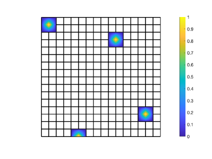
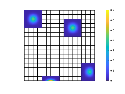
$p=1$                                                              $p=3$

Figure 1. B-splines of degree $p=1,3$ and maximal smoothness $p-1$ on a two-dimensional uniform tensor mesh $\mathcal{T}_{h}$.

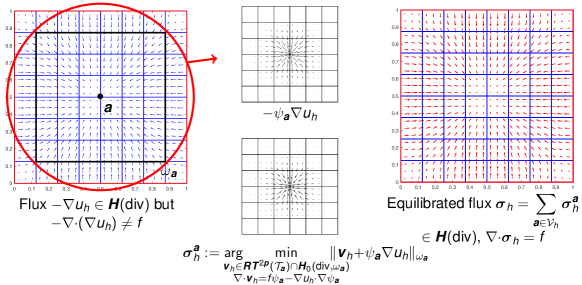
Figure 2. A straightforward (expensive) extension of the FEM equilibration to IGA with B-splines of degree $p=5$ and maximal smoothness $p-1$ on a two-dimensional uniform tensor mesh $\mathcal{T}_{h}$.

3.3. Inexpensive equilibration in IGA

Our main idea is to replace the straightforward approach of Section 3.2 by a construction that does not request the expensive solution of (9) employing the large spaces $\bm{V}_{h}^{{\bm{a}}}$ of (8) defined over the large spline supports $\omega_{\bm{a}}$. We design a two-stage procedure where: first, lowest-order $\mathbb{Q}^{\bm{1}}(\mathcal{T}_{\bm{a}})\cap C^{0}(\omega_{\bm{a}})$ scalar problems are solved on each large patch $\mathcal{T}_{\bm{a}}$; second, systems of the form (9), but only over the finite element hat basis functions supports $\omega_{\bm{b}}$ with $2^{d}$ mesh elements, are solved. This is schematically viewed in Figure 3. Similar $p$-robust constructions were designed in [SMPZ08] in the context of an additive Schwarz smoother/preconditiner (just one global lowest-order solve and then $p$-order local patch problems) or in [ESV17a, ESV17b, PV22] for a posteriori error estimates (allowing for fast equilibration with $H^{-1}(\Omega)$ right-hand sides/arbitrary coarsening in parabolic time stepping/inexpensive estimates of the algebraic error).

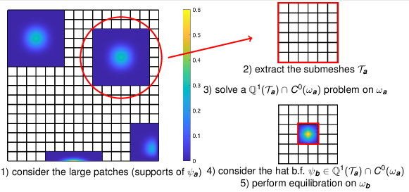
Figure 3. Inexpensive equilibration in IGA in the simplified setting of uniform tensor-product mesh, $p=5$ and maximal smoothness $p-1$.

More precisely, we first, on each (large) patch subdomain $\omega_{\bm{a}}$ with local mesh $\mathcal{T}_{\bm{a}}$ solve the primal lowest-order problem: find

$$r_{h}^{\bm{a}}\in V_{h}^{\bm{a}}:=\begin{cases}\{v_{h}\in\mathbb{Q}^{1}(\mathcal{T}_{\bm{a}})\cap C^{0}(\omega_{\bm{a}})\,:\,(v_{h}\,,\,1)_{\omega_{\bm{a}}}=0\}\quad&\text{if }\psi_{\bm{a}}\in H_{0}^{1}(\Omega),\\ \{v_{h}\in\mathbb{Q}^{1}(\mathcal{T}_{\bm{a}})\cap C^{0}(\omega_{\bm{a}})\,:\,v_{h}=0\text{ on }\partial\omega_{\bm{a}}\setminus\psi_{\bm{a}}^{-1}(\{0\})\}\quad&\text{else}\end{cases}$$

such that

$$(\nabla r_{h}^{\bm{a}}\,,\,\nabla v_{h})_{\omega_{\bm{a}}}=(f\,,\,v_{h}\psi_{\bm{a}})_{\omega_{\bm{a}}}-(\nabla u_{h}\,,\,\nabla(v_{h}\psi_{\bm{a}}))_{\omega_{\bm{a}}}\quad\text{for all }v_{h}\in V_{h}^{\bm{a}},$$ (12)

see Figure 3, steps 1)–3). This yields the scalar-valued lifting $r_{h}^{\bm{a}}$ of the $\psi_{\bm{a}}$-weighted residual of (3) with respect to (2). Second, we consider the finite element hat basis functions $\psi_{\bm{b}}$ of vertices ${\bm{b}}$ of the local mesh $\mathcal{T}_{\bm{a}}$ and solve the dual high-order problems

$$\bm{\sigma}_{h}^{{\bm{a}},{\bm{b}}}:=\underset{\begin{subarray}{c}\bm{v}_{h}\in\bm{V}_{h}^{{\bm{a}},{\bm{b}}}\\ \nabla{\cdot}\bm{v}_{h}=f\psi_{\bm{a}}\psi_{\bm{b}}-\nabla u_{h}{\cdot}\nabla(\psi_{\bm{a}}\psi_{\bm{b}})-\nabla r_{h}^{\bm{a}}{\cdot}\nabla\psi_{\bm{b}}\end{subarray}}{\operatorname{argmin}}\|\bm{v}_{h}+\psi_{\bm{b}}(\psi_{\bm{a}}\nabla u_{h}+\nabla r_{h}^{\bm{a}})\|_{\omega_{\bm{b}}},$$ (13)

where $\bm{V}_{h}^{{\bm{a}},{\bm{b}}}$ is defined similarly to (8), with

$$\bm{H}_{0}(\mathrm{div},\omega_{\bm{b}}):=\begin{cases}\{\bm{v}\in\bm{H}(\mathrm{div},\omega_{\bm{b}})\,:\,\bm{v}{\cdot}\bm{n}_{\omega_{\bm{b}}}=0\text{ on }\partial\omega_{\bm{b}}\}&\text{if }\psi_{\bm{a}}\psi_{\bm{b}}\in H_{0}^{1}(\Omega),\\ \{\bm{v}\in\bm{H}(\mathrm{div},\omega_{\bm{b}})\,:\,\bm{v}{\cdot}\bm{n}_{\omega_{\bm{b}}}=0\text{ on }\partial\omega_{\bm{b}}\\ \hskip 142.26378pt\cap(\psi_{\bm{a}}\psi_{\bm{b}})^{-1}(\{0\})\}&\text{else},\\ \end{cases}$$

see Figure 3, steps 4)–5). As in Section 3.2, we need to increase the equilibration polynomial degree $\widetilde{\bm{p}}$; actually, owing to the presence of the finite element hat basis function $\psi_{\bm{b}}$, we will need $\widetilde{\bm{p}}=2\bm{p}+1$ and not just $\widetilde{\bm{p}}=2\bm{p}$ to satisfy $\psi_{\bm{b}}(\psi_{\bm{a}}\nabla u_{h}+\nabla r_{h}^{\bm{a}})\in\bm{RT}^{\widetilde{\bm{p}}}(\mathcal{T}_{\bm{a}})$ and $f\psi_{\bm{a}}\psi_{\bm{b}}-\nabla u_{h}{\cdot}\nabla(\psi_{\bm{a}}\psi_{\bm{b}})-\nabla r_{h}^{\bm{a}}{\cdot}\nabla\psi_{\bm{b}}\in\mathbb{Q}^{\widetilde{\bm{p}}}(\mathcal{T}_{\bm{a}})$ to avoid all oscillation terms. All these local problems can be solved independently one from each other, allowing for efficient parallelization. Moreover, for every two same patch geometries, one matrix assembly and factorization is sufficient.

To finish, we sum the contributions $\bm{\sigma}_{h}^{{\bm{a}},{\bm{b}}}$ from (13) as

$$\bm{\sigma}_{h}^{\bm{a}}:=\sum_{{\bm{b}}\in\mathcal{V}_{h}^{\bm{a}}}\bm{\sigma}_{h}^{{\bm{a}},{\bm{b}}}$$ (14)

and form the final equilibrated flux as

$$\bm{\sigma}_{h}:=\sum_{{\bm{a}}\in\mathcal{V}_{h}}\bm{\sigma}_{h}^{\bm{a}},$$ (15)

which yields a fully computable guaranteed (constant-free in the leading term) upper bound on the unknown error similarly to (10), see Proposition 8.2 for details. This bound is also locally and globally efficient, see respectively Propositions 8.4 and 8.6. The involved constant $C_{\rm eff}$ is robust with respect to the polynomial degree $p$ of the used hierarchical splines and the number of hanging nodes of the underlying hierarchical meshes, but theoretically not with respect to the smoothness of the splines and the number of patches $\omega_{\bm{a}}$ overlapping in a point (see (84a)) (in our numerical experiments, though, $C_{\rm eff}$ shows robustness with respect to the smoothness and the number of overlapping patches). Full details of the equilibration are given in Definitions 7.1, 7.2, and 7.5 below; Figure 6 illustrates the procedure on hierarchical meshes.

4. Hierarchical splines

In this section, we first describe the piecewise polynomial space of multivariate splines in the parameter domain $\widehat{\Omega}$. We then introduce its hierarchical extension, covering highly graded local mesh refinement. Finally, the space $V_{h}$ from (3) will be given by the transformation of the latter one by the mapping $\bm{F}$.

4.1. Multivariate splines in the parameter domain $(0,1)^{d}$

We recall here the standard definition of multivariate splines in the parameter domain $(0,1)^{d}$; for a detailed introduction, we refer, e.g., to [dB86, dB01, Sch07].

Let the integer $p\geq 1$ be a fixed positive polynomial degree and let

$${\mathcal{K}}_{h}=(\mathcal{K}_{1(h)},\dots,\mathcal{K}_{d(h)})$$

be a fixed $d$-dimensional vector of $p$-open knot vectors, i.e., for each spatial dimension $1\leq i\leq d$,

$$\mathcal{K}_{i(h)}=(t_{i(h),0},\dots,t_{i(h),N_{i(h)}+p})$$

is a $p$-open knot vector in $[0,1]$, which means that

$$0=t_{i(h),0}=\dots=t_{i(h),p}<t_{i(h),p+1}\leq t_{i(h),p+2}\dots<t_{i(h),N_{i(h)}}=\dots=t_{i(h),N_{i(h)}+p}=1.$$

Moreover, we assume that each of the interior knots $t_{i(h),j}\in(0,1)$ appears at most with multiplicity $p$. By definition, the boundary knots $0$ and $1$ have multiplicity $p+1$. An example is given in Figure 4, with polynomial degree $p=2$, number of knots minus $p$ minus one $=$ $N_{i(h)}=9$ (this will later correspond to the dimension of the B-splines space), and a varying multiplicity.

We define the resulting one-dimensional meshes

$$\widehat{\mathcal{T}}_{i(h)}:=\{[t_{i(h),j-1},t_{i(h),j}]\,:\,j\in\{1,\dots,N_{i(h)}+p\}\wedge t_{i(h),j-1}<t_{i(h),j}\},\quad i=1,\dots,d,$$

as well as the resulting tensor mesh

$$\widehat{\mathcal{T}}_{h}:=\{\widehat{T}_{1}\times\dots\times\widehat{T}_{d}\,:\,\widehat{T}_{i}\in\widehat{\mathcal{T}}_{i(h)}\text{ for all }i\in\{1,\dots,d\}\}.$$

By ${\mathbb{S}}^{p}(\mathcal{K}_{i(h)})$, we denote the set of all corresponding univariate splines, i.e., the set of all $\widehat{\mathcal{T}}_{i(h)}$-piecewise univariate polynomials of degree $p$ that are $p-\#t_{i(h),j}$-times continuously differentiable at any interior knot $t_{i(h),j}$, where $\#t_{i(h),j}$ denotes the corresponding multiplicity of $t_{i(h),j}$ within $\mathcal{K}_{i(h)}$. Assuming for example that all interior multiplicities are equal to $p$, ${\mathbb{S}}^{p}(\mathcal{K}_{i(h)})$ is just the space of all $\widehat{\mathcal{T}}_{i(h)}$-piecewise univariate polynomials of degree $p$ that are merely continuous, i.e., $C^{0}(0,1)$, cf. (4). At the other extreme, when all interior multiplicities are equal to $1$, then ${\mathbb{S}}^{p}(\mathcal{K}_{i(h)})$ is the space of $\widehat{\mathcal{T}}_{i(h)}$-piecewise univariate polynomials of degree $p$ with continuous derivatives up to order $p-1$, cf. (11) with $m=1$. We refer again to Figure 4 for an example.

A basis of ${\mathbb{S}}^{p}(\mathcal{K}_{i(h)})$, of dimension $N_{i(h)}$, is given by the set of B-splines

$$\{B_{i(h),j,p}\,:\,j\in\{1,\dots,N_{i(h)}\}\},$$

where the B-splines $B_{i(h),j,p}$ are recursively defined for all points $t\in(0,1)$ via

$$B_{i(h),j,0}(t):=\begin{cases}1\quad&\text{if }t_{i(h),j}\leq t<t_{i(h),j+1},\\ 0\quad&\text{else},\end{cases}$$ (16a)

and

$$B_{i(h),j,p}(t):=\frac{t-t_{i(h),j}}{t_{i(h),j+p}-t_{i(h),j}}B_{i(h),j,p-1}(t)+\frac{t_{i(h),j+p+1}-t}{t_{i(h),j+p+1}-t_{i(h),j+1}}B_{i(h),j+1,p-1}(t)$$ (16b)

with the formal convention that $\cdot/0:=0$. Figure 4 gives an illustrative example, where the $N_{i(h)}=9$ basis functions are depicted. It is easy to see that the support is

$$\mathrm{supp}(B_{i(h),j,p})=[t_{i(h),j},t_{i(h),j+p+1}]$$ (17)

and we also remark that

$$0\leq B_{i(h),j,p}\leq 1.$$ (18)

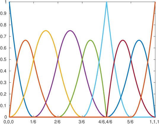
Figure 4. The B-splines of degree $p=2$ corresponding to the knot vector $\mathcal{K}=(0,0,0,1/6,2/6,3/6,4/6,4/6,5/6,1,1,1)$ are depicted. They are at least $C^{1}$ at the knots $1/6,2/6,3/6,$ and $5/6$, and at least $C^{0}$ at $4/6$.

We abbreviate $\bm{p}:=(p,\dots,p)\in\mathbb{N}^{d}$. The space ${\mathbb{S}}^{\bm{p}}(\mathcal{K}_{h})$ of multivariate splines is defined as tensor-product of the univariate spline spaces. Note that each function in ${\mathbb{S}}^{\bm{p}}(\mathcal{K}_{h})$ is a $\widehat{\mathcal{T}}_{h}$-piecewise multivariate polynomial of degree $\bm{p}$. Again, assuming for example that all interior knots have multiplicity $p$, ${\mathbb{S}}^{\bm{p}}(\mathcal{K}_{h})$ is just the space of all continuous $\widehat{\mathcal{T}}_{h}$-piecewise multivariate polynomials of degree $\bm{p}$, i.e., up to boundary conditions, (4), while multiplicity $1$ of all interior knots yields the space of all $\widehat{\mathcal{T}}_{h}$-piecewise multivariate polynomials of degree $\bm{p}$ with continuous derivatives up to order $p-1$, i.e., up to boundary conditions, (11) for $m=1$. Clearly, the set of tensor-products of the univariate B-splines

$$\{B_{h,\bm{j},\bm{p}}\,:\,\bm{j}\in\Pi_{i=1}^{d}\{1,\dots,N_{i(h)}\}\}\quad\text{with}\quad B_{h,\bm{j},\bm{p}}(\bm{t}):=\Pi_{i=1}^{d}B_{i(h),j_{i},p}(t_{i}),$$ (19)

provides a basis of ${\mathbb{S}}^{\bm{p}}(\mathcal{K}_{h})$.

4.2. Hierarchical splines in the parameter domain $(0,1)^{d}$

We now introduce hierarchical splines, which are defined on a hierarchical mesh and are essentially coarse splines on coarse mesh elements and fine splines on fine mesh elements. For a detailed introduction, we refer, e.g., to the seminal work [VGJS11].

Let $p$ be a fixed positive polynomial degree as above and let ${\mathcal{K}}_{0}=(\mathcal{K}_{1(0)},\dots,\mathcal{K}_{d(0)})$ be a fixed initial $d$-dimensional vector of $p$-open knot vectors in $[0,1]$ with interior multiplicities less than or equal to $p$, as in Section 4.1. Recall that we consider $d=2,3$. We set $\mathcal{K}_{{\rm uni}(0)}:=\mathcal{K}_{0}$ and recursively define $\mathcal{K}_{{\rm uni}(\ell+1)}$ for $\ell\in\mathbb{N}_{0}$ as the uniform $h$-refinement of $\mathcal{K}_{{\rm uni}(\ell)}$ with fixed multiplicity $m\in\mathbb{N}$, i.e., obtained by inserting the knot $(t_{i({\rm uni}(\ell)),j-1}+t_{i({\rm uni}(\ell)),j})/{2}$ to the knots $\mathcal{K}_{i({\rm uni}(\ell))}$ with multiplicity $m$ whenever $t_{i({\rm uni}(\ell)),j-1}<t_{i({\rm uni}(\ell)),j}$. We use analogous notation as in Section 4.1, replacing the index $h$ by ${\rm uni}(\ell)$, e.g., we write $\widehat{\mathcal{T}}_{{\rm uni}(\ell)}$ for the induced tensor mesh. We stress that these spline spaces are nested in the sense that

$${\mathbb{S}}^{\bm{p}}(\mathcal{K}_{{\rm uni}(\ell)})\subset{\mathbb{S}}^{\bm{p}}(\mathcal{K}_{{\rm uni}(\ell+1)})\subset C^{0}((0,1)^{d}),$$ (20)

where the last relation follows from the assumption that multiplicities of interior knots is less than or equal to $p$.

Remark 4.1.

As a matter of fact, the definition of the uniform refinements $\mathcal{K}_{{\rm uni}(\ell)}$ allows for a certain flexibility without changing the results of the present manuscript. For instance, instead of the natural dyadic uniform refinement, one could use $n$-adic refinement, i.e., insert the knots $(t_{i({\rm uni}(\ell)),j-1}+t_{i({\rm uni}(\ell)),j})/{n},\dots,(n-1)(t_{i({\rm uni}(\ell)),j-1}+t_{i({\rm uni}(\ell)),j})/{n}$ to the knots $\mathcal{K}_{i({\rm uni}(\ell))}$ with multiplicity $m$ whenever $t_{i({\rm uni}(\ell)),j-1}<t_{i({\rm uni}(\ell)),j}$.

We say that a set

$$\widehat{\mathcal{T}}_{h}\subseteq\bigcup_{\ell\in\mathbb{N}_{0}}\widehat{\mathcal{T}}_{{\rm uni}(\ell)}$$

is a hierarchical mesh if it is a partition of $[0,1]^{d}$ in the sense that $\bigcup\widehat{\mathcal{T}}_{h}=[0,1]^{d}$, where the intersection of two different elements $\widehat{T}\neq\widehat{T}^{\prime}$ with $\widehat{T},\widehat{T}^{\prime}\in\widehat{\mathcal{T}}_{h}$ has ($d$-dimensional) measure zero. Since $\widehat{\mathcal{T}}_{{\rm uni}(\ell)}\cap\widehat{\mathcal{T}}_{{\rm uni}(\ell^{\prime})}=\emptyset$ for $\ell,\ell^{\prime}\in\mathbb{N}_{0}$ with $\ell\neq\ell^{\prime}$, we can define for any element $\widehat{T}\in\widehat{\mathcal{T}}_{h}$,

$$\mathrm{level}(\widehat{T}):=\ell\in\mathbb{N}_{0}\quad\text{with }\widehat{T}\in\widehat{\mathcal{T}}_{{\rm uni}(\ell)}.$$

For an illustrative example of a hierarchical mesh, see Figure 5. In particular, any uniformly refined tensor mesh $\widehat{\mathcal{T}}_{{\rm uni}(\ell)}$ with $\ell\in\mathbb{N}_{0}$ is a hierarchical mesh.

For a hierarchical mesh $\widehat{\mathcal{T}}_{h}$, we define a corresponding nested sequence $(\widehat{\Omega}^{\ell}_{h})_{\ell\in\mathbb{N}_{0}}$ of closed subsets of $[0,1]^{d}$ as

$$\widehat{\Omega}_{h}^{\ell}:=\bigcup_{\ell^{\prime}\geq\ell}\big{(}\widehat{\mathcal{T}}_{h}\cap\widehat{\mathcal{T}}_{{\rm uni}(\ell^{\prime})}\big{)},$$

i.e., $\widehat{\Omega}_{h}^{\ell}$ covers all elements with level greater than or equal to $\ell$. Note that there exists a minimal integer $L_{h}$ such that $\widehat{\Omega}_{h}^{\ell}=\emptyset$ for all $\ell\geq L_{h}$. It holds that

$$\widehat{\mathcal{T}}_{h}=\bigcup_{\ell\in\mathbb{N}_{0}}\{\widehat{T}\in\widehat{\mathcal{T}}_{{\rm uni}(\ell)}\,:\,\widehat{T}\subseteq\widehat{\Omega}_{h}^{\ell}\wedge\widehat{T}\not\subseteq\widehat{\Omega}_{h}^{\ell+1}\}.$$ (21)

In the literature, one usually assumes that the sequence $(\widehat{\Omega}^{\ell}_{h})_{\ell\in\mathbb{N}_{0}}$ is given and the corresponding hierarchical mesh is defined via (21).

Figure 5. A two-dimensional hierarchical mesh $\widehat{\mathcal{T}}_{h}$ with level of all elements less than $4$. Levels $0$ to $3$ are respectively highlighted in white, light grey, grey, and dark grey, also denoting the corresponding domains $\widehat{\Omega}^{0}_{h}\setminus\widehat{\Omega}^{1}_{h}$, $\widehat{\Omega}^{1}_{h}\setminus\widehat{\Omega}^{2}_{h}$, $\widehat{\Omega}^{2}_{h}\setminus\widehat{\Omega}^{3}_{h}$, $\widehat{\Omega}^{3}_{h}\setminus\widehat{\Omega}^{4}_{h}$; $\widehat{\Omega}_{h}^{4}=\emptyset$.

We introduce the hierarchical basis

$$\{B_{\bm{a}}\,:\,{\bm{a}}\in\mathcal{I}_{h}\}\quad\text{with }\quad\mathcal{I}_{h}:=\bigcup_{\ell\in\mathbb{N}_{0}}\Big{\{} ({\rm uni}(\ell),\bm{j},\bm{p}):\bm{j}\in\Pi_{i=1}^{d}\{1,\dots,N_{i({\rm uni}(\ell))}\}$$ (22)

$$\wedge\mathrm{supp}(B_{{\rm uni}(\ell),\bm{j},\bm{p}})\subseteq\widehat{\Omega}_{h}^{\ell}\wedge\mathrm{supp}(B_{{\rm uni}(\ell),\bm{j},\bm{p}})\not\subseteq\widehat{\Omega}_{h}^{\ell+1}\Big{\}},$$

where we recall the definition (19) of a multivariate B-spline. Figure 6 gives an illustrative example. Its elements are referred to as (multivariate) hierarchical B-splines. For ${\bm{a}}\in\mathcal{I}_{h}$, the level of the corresponding hierarchical B-spline is well defined

$$\mathrm{level}(B_{\bm{a}}):=\ell\in\mathbb{N}_{0}\quad\text{with }{\bm{a}}=({\rm uni}(\ell),\bm{j},\bm{p}).$$ (23)

It is easy to check that if $\widehat{\mathcal{T}}_{h}$ is a tensor mesh, and hence coincides with some $\widehat{\mathcal{T}}_{{\rm uni}(\ell)}$, then the hierarchical basis and the standard tensor-product B-spline basis are the same. One can prove that the hierarchical B-splines are linearly independent; see, e.g., [VGJS11, Lemma 2]. They span the space of hierarchical splines

$${\mathbb{S}}^{\bm{p}}(\mathcal{K}_{0},m,\widehat{\mathcal{T}}_{h}):={\rm span}\big{(}\{B_{\bm{a}}\,:\,{\bm{a}}\in\mathcal{I}_{h}\}\big{)}.$$ (24)

(a)

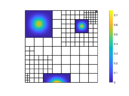
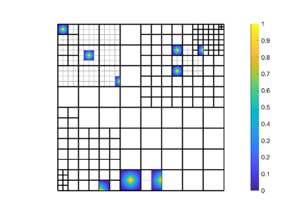
(b)                                                              (c)

Figure 6. A two-dimensional hierarchical mesh $\widehat{\mathcal{T}}_{h}$ (of Figure 5) is depicted in black. Assuming that all interior knots have multiplicity $1$, in (a), the support of three hierarchical B-splines of degree $p=2$ is highlighted in blue; two hierarchical B-splines of level $0$ (left and bottom), and one hierarchical B-spline of level $1$ (right). The corresponding local tensor meshes $\widehat{\mathcal{T}}_{\bm{a}}$ are indicated in grey. In (b), these three hierarchical B-splines are depicted. For $\overline{p}=2$, these functions also belong (up to scaling) to the partition of unity $\{\psi_{\bm{a}}\circ\bm{F}\,:\,{\bm{a}}\in\mathcal{V}_{h}\}$ defined in Section 5.1 below. Finally, in (c), for each of them, three functions of the corresponding local partition of unity $\{\psi_{\bm{b}}\circ\bm{F}\,:\,{\bm{b}}\in\mathcal{V}_{h}^{\bm{a}}\}$ defined in Section 5.1 below over the local tensor meshes are depicted.

The hierarchical basis and the mesh $\widehat{\mathcal{T}}_{h}$ are compatible in the following sense: For all $B_{\bm{a}}$, ${\bm{a}}\in\mathcal{I}_{h}$, the corresponding support can be written as union of elements in $\widehat{\mathcal{T}}_{{\rm uni}(\mathrm{level}(B_{\bm{a}}))}$, i.e.,

$$\mathrm{supp}(B_{\bm{a}})=\bigcup\{\widehat{T}\in\widehat{\mathcal{T}}_{{\rm uni}(\mathrm{level}(B_{\bm{a}}))}\,:\,\widehat{T}\subseteq\mathrm{supp}(B_{\bm{a}})\}.$$

Each such element $\widehat{T}\in\widehat{\mathcal{T}}_{{\rm uni}(\mathrm{level}(B_{\bm{a}}))}$ with $\widehat{T}\subseteq\mathrm{supp}(B_{\bm{a}})\subseteq\widehat{\Omega}_{h}^{\mathrm{level}(B_{\bm{a}})}$ satisfies that $\widehat{T}\in\widehat{\mathcal{T}}_{h}$ or $\widehat{T}\subseteq\widehat{\Omega}_{h}^{\mathrm{level}(B_{\bm{a}})+1}$. In either case, we see that $\widehat{T}$ can be written as union of elements in $\widehat{\mathcal{T}}_{h}$ with level greater or equal to $\mathrm{level}(B_{\bm{a}})$. Altogether, we have that

$$\mathrm{supp}(B_{\bm{a}})=\bigcup_{\ell\geq\mathrm{level}(B_{\bm{a}})}\{\widehat{T}\in\widehat{\mathcal{T}}_{h}\cap\widehat{\mathcal{T}}_{{\rm uni}(\ell)}\,:\,\widehat{T}\subseteq\mathrm{supp}(B_{\bm{a}})\}.$$ (25)

Moreover, $\mathrm{supp}(B_{\bm{a}})$ must contain at least one element of $\mathrm{level}(B_{\bm{a}})$. Otherwise one would get the contradiction $\mathrm{supp}(B_{\bm{a}})\subseteq\widehat{\Omega}_{h}^{\mathrm{level}(B_{\bm{a}})+1}$.

We now present the following characterization of hierarchical splines, which has been verified in [SM16, Section 3],

$$\begin{split}{\mathbb{S}}^{\bm{p}}(\mathcal{K}_{0},m,\widehat{\mathcal{T}}_{h})=\big{\{}\widehat{v}_{h}:(0,1)^{d}\to\mathbb{R}:\widehat{v}_{h}|_{(0,1)^{d}\setminus\widehat{\Omega}_{h}^{\ell+1}}\in\mathbb{S}^{\bm{p}}(\mathcal{K}_{{\rm uni}(\ell)})|_{(0,1)^{d}\setminus\widehat{\Omega}_{h}^{\ell+1}}\text{ for all }\ell\in\mathbb{N}_{0}\big{\}}.\end{split}$$ (26)

In particular, each hierarchical spline is a $\widehat{\mathcal{T}}_{h}$-piecewise tensor-product polynomial of degree $\bm{p}$. Put into words, hierarchical splines are coarse splines on coarse mesh elements, and they are fine splines on fine mesh elements.

Finally, we say that a hierarchical mesh $\widehat{\mathcal{T}}_{h}$ is finer than another hierarchical mesh $\widehat{\mathcal{T}}_{H}$ if $\widehat{\mathcal{T}}_{h}$ is obtained from $\widehat{\mathcal{T}}_{H}$ via iterative dyadic bisection. Formally, this can be stated as $\widehat{\Omega}_{H}^{\ell}\subseteq\widehat{\Omega}_{h}^{\ell}$ for all $\ell\in\mathbb{N}_{0}$. In this case, (26) shows that the corresponding hierarchical spline spaces are nested, i.e.,

$${\mathbb{S}}^{\bm{p}}(\mathcal{K}_{0},m,\widehat{\mathcal{T}}_{H})\subseteq{\mathbb{S}}^{\bm{p}}(\mathcal{K}_{0},m,\widehat{\mathcal{T}}_{h}).$$ (27)

In particular, we see that

$${\mathbb{S}}^{\bm{p}}(\mathcal{K}_{{\rm uni}(0)})\subseteq{\mathbb{S}}^{\bm{p}}(\mathcal{K}_{0},m,\widehat{\mathcal{T}}_{h})\subseteq{\mathbb{S}}^{\bm{p}}(\mathcal{K}_{{\rm uni}(L_{h}-1)}).$$

4.3. Hierarchical splines in the physical domain $\Omega$

If $\widehat{\mathcal{T}}_{h}$ is a hierarchical mesh in the parameter domain $(0,1)^{d}$, we set

$$\mathcal{T}_{h}:=\{\bm{F}(\widehat{T})\,:\,\widehat{T}\in\widehat{\mathcal{T}}_{h}\},$$

where $\bm{F}$ is the bi-Lipschitz mapping from Section 2. In this context, $h\in L^{\infty}(\Omega)$ denotes the mesh size function defined by $h|_{T}:=\mathrm{diam}(T)$ for all $T\in\mathcal{T}_{h}$. Moreover, we set

$${\mathbb{S}}^{\bm{p}}(\mathcal{K}_{0},m,\mathcal{T}_{h}):=\{\widehat{v}\circ\bm{F}^{-1}\,:\,\widehat{v}\in{\mathbb{S}}^{\bm{p}}(\mathcal{K}_{0},m,\widehat{\mathcal{T}}_{h})\}.$$

The conforming ansatz space for the Galerkin discretization (3) is then defined as

$$V_{h}:={\mathbb{S}}^{\bm{p}}(\mathcal{K}_{0},m,\mathcal{T}_{h})\cap H_{0}^{1}(\Omega).$$ (28)

Remark 4.2.

In practice, the parametrization $\bm{F}$ is often given in terms of non-uniform rational B-splines (NURBS) along with corresponding polynomial degree $\bm{p}_{\bm{F}}$ and global knot vector $\mathcal{K}_{\bm{F}}$. To guarantee good approximation properties of $V_{h}$, in particular good a priori estimates, the functions in ${\mathbb{S}}^{\bm{p}}(\mathcal{K}_{0},m,\widehat{\mathcal{T}}_{h})$ should have the same or lower smoothness as $\bm{F}$ along the knot lines on $\widehat{\Omega}$ corresponding to $\mathcal{K}_{\bm{F}}$. Such a requirement is not needed for the presented a posteriori error analysis to hold. Moreover, the form of the oscillation terms (77b) and (84c) for reliability and efficiency, respectively, suggests that the approximation property of $V_{h}$ has minor influence on the size of these terms, see also Remark 5.1.

5. Partitions of unity and patchwise spaces

In this section, we prepare the necessary material for defining and analyzing our equilibrated fluxes in the IGA context later. We particularly design a partition of unity based on hierarchical B-splines and define continuous- and discrete-level local spaces.

5.1. Partitions of unity based on hierarchical splines

We now first construct a partition of unity on $\Omega$ consisting of hierarchical B-splines with the smallest-possible polynomial degree $\overline{p}$ but sufficient smoothness to be contained in ${\mathbb{S}}^{\bm{p}}(\mathcal{K}_{0},m,\mathcal{T}_{h})$. Subsequently, on the local tensor meshes of the support of each of these hierarchical B-splines, we form a partition of unity by piecewise multilinear hat functions with merely $C^{0}(\Omega)$ continuity.

Let $\overline{p}\leq p$ be a supplementary polynomial degree and let

$${\overline{\mathcal{K}}}_{0}=(\overline{\mathcal{K}}_{1(0)},\dots,\overline{\mathcal{K}}_{d(0)})$$

be a fixed $d$-dimensional vector of $\overline{p}$-open knot vectors

$$\overline{\mathcal{K}}_{i(0)}=(\overline{t}_{i(0),0},\dots,\overline{t}_{i(0),\overline{N}_{i(0)}+\overline{p}})$$

such that $(\overline{t}_{i(0),\overline{p}},\dots,\overline{t}_{i(0),\overline{N}_{i(0)}})$ is a subsequence of $(t_{i(0),p},\dots,t_{i(0),N_{i(0)}})$ which is obtained by reducing multiplicities of the latter knots to at least one and

$$0=\overline{t}_{i(0),0}=\dots=\overline{t}_{i(0),\overline{p}}\quad\text{and}\quad\overline{t}_{i(0),\overline{N}_{i(0)}}=\dots=\overline{t}_{i(0),\overline{N}_{i(h)}+\overline{p}}=1.$$

In particular, the tensor mesh corresponding to $\overline{\mathcal{K}}_{0}$ coincides with the initial tensor-mesh $\widehat{\mathcal{T}}_{0}$ corresponding to $\mathcal{K}_{0}$. To guarantee that

$${\mathbb{S}}^{\overline{p}}(\overline{\mathcal{K}}_{i(0)})\subseteq{\mathbb{S}}^{p}(\mathcal{K}_{i(0)}),$$ (29)

we further suppose that

$$p-\#t_{i(0),j}\leq\overline{p}-\overline{\#}t_{i(0),j}$$ (30)

for all interior knots $t_{i(0),j}$ in $(0,1)$ (which determines the smoothness of the considered splines), where $\overline{\#}$ denotes the multiplicity within $\overline{\mathcal{K}}_{i(0)}$. Next, we set $\overline{\mathcal{K}}_{{\rm uni}(0)}:=\overline{\mathcal{K}}_{0}$ and recursively define $\overline{\mathcal{K}}_{{\rm uni}(\ell+1)}$ for $\ell\in\mathbb{N}_{0}$ as the uniform $h$-refinement of $\overline{\mathcal{K}}_{{\rm uni}(\ell)}$ with fixed multiplicity $\overline{m}\in\mathbb{N}$ such that

$$p-m\leq\overline{p}-\overline{m}.$$ (31)

In words, the knots of $\overline{\mathcal{K}}_{{\rm uni}(\ell+1)}$ in $[0,1]$ are the knots of $\overline{\mathcal{K}}_{{\rm uni}(\ell)}$ in $[0,1]$ plus the points $(t_{i({\rm uni}(\ell)),j-1}+t_{i({\rm uni}(\ell)),j})/{2}$ with multiplicity $\overline{m}$ if $t_{i({\rm uni}(\ell)),j-1}<t_{i({\rm uni}(\ell)),j}$ for $j\in\{\overline{p}+1,\dots,\overline{N}_{i({\rm uni}(\ell))}\}$. If, for example, all interior knots in $\mathcal{K}_{0}$ have the same multiplicity $1$ and $m=1$, i.e., the corresponding splines are $C^{p-1}$ along initial as well as new lines, one can only choose $\overline{p}=p$ and $\overline{m}=1$. If all interior knots in $\mathcal{K}_{0}$ have the same multiplicity $p$ and $m=p$, i.e., the corresponding splines are only $C^{0}$ along initial as well as new lines, one can choose $\overline{p}\leq p$ and $\overline{m}\leq\overline{p}$ arbitrarily, which leads us to $\overline{p}=1$ and $\overline{m}=1$. While the analysis below does not rely on this, we will always choose the smallest-possible polynomial degree $\overline{p}$ together with $\overline{m}:=1$. This is the most sensible choice from a practical as well as theoretical point of view, as the efficiency constant of our estimator depends on the degree $\overline{p}$; see Proposition 6.9 and Remark 6.10 as well as Proposition 8.6 and Remark 8.7 below. In Remark 8.8, we further discuss that the choice of $\overline{p}$ and $\overline{m}$ has little influence on the data oscillation terms arising in our error estimator.

Let again $\widehat{\mathcal{T}}_{h}$ be a hierarchical mesh with corresponding sets $(\widehat{\Omega}_{h}^{\ell})_{\ell\in\mathbb{N}_{0}}$ as in Section 4.2. Setting $\overline{\bm{p}}:=(\overline{p},\dots,\overline{p})$, we define the B-splines $\overline{B}_{({\rm uni}(\ell),\bm{j},\overline{\bm{p}})}$, the hierarchical basis $\{\overline{B}_{\bm{a}}\,:\,{\bm{a}}\in\overline{\mathcal{I}}_{h}\}$ with index set $\overline{\mathcal{I}}_{h}$, the level $\mathrm{level}(\overline{B}_{\bm{a}})$ for ${\bm{a}}\in\mathcal{I}_{h}$, and the spanned space of hierarchical splines ${\mathbb{S}}^{\bm{p}}(\overline{\mathcal{K}}_{0},\overline{m},\widehat{\mathcal{T}}_{h})$ as in (22)–(24). Again, [SM16, Section 3] gives an explicit characterization for the spanned space of hierarchical splines. Our assumptions on the knot multiplicities, which imply the nestedness $\mathbb{S}^{\overline{\bm{p}}}(\overline{\mathcal{K}}_{{\rm uni}(\ell)})\subseteq\mathbb{S}^{\bm{p}}(\mathcal{K}_{{\rm uni}(\ell)})$ for all $\ell\in\mathbb{N}_{0}$, thus give that

$${\mathbb{S}}^{\overline{\bm{p}}}({\overline{\mathcal{K}}}_{0},\overline{m},\widehat{\mathcal{T}}_{h})\subseteq{\mathbb{S}}^{\bm{p}}({\mathcal{K}}_{0},m,\widehat{\mathcal{T}}_{h}).$$ (32)

Now $1\in{\mathbb{S}}^{\overline{\bm{p}}}(\overline{\mathcal{K}}_{0},\overline{m},\widehat{\mathcal{T}}_{h})$ yields the existence of a partition of unity on the parameter domain

$$1=\sum_{{\bm{a}}\in\overline{\mathcal{I}}_{h}}c_{\bm{a}}\overline{B}_{\bm{a}}.$$

One can prove that the coefficients $c_{\bm{a}}\in\mathbb{R}$ satisfy that

$$0\leq c_{\bm{a}}\leq 1$$ (33)

for all ${\bm{a}}\in\overline{\mathcal{I}}_{h}$; see, e.g., [BG16a, Lemma 3.2]. Consequently, we can define

$$\psi_{\bm{a}}:=(c_{\bm{a}}\overline{B}_{\bm{a}})\circ\bm{F}^{-1}\quad\text{for all }{\bm{a}}\in\mathcal{V}_{h}:=\{{\bm{a}}\in\overline{\mathcal{I}}_{h}\,:\,c_{\bm{a}}>0\}$$ (34)

and observe that the $\psi_{\bm{a}}$ form a partition of unity on the physical domain

$$\sum_{{\bm{a}}\in\mathcal{V}_{h}}\psi_{\bm{a}}=1\quad\text{in }\Omega.$$

Henceforth, we call $\mathcal{V}_{h}$ the set of nodes and ${\bm{a}}\in\mathcal{V}_{h}$ a node. For further use, we abbreviate $\omega_{\bm{a}}:={\rm int}(\mathrm{supp}(\psi_{\bm{a}}))$ as well as $\widehat{\omega}_{\bm{a}}:=\bm{F}^{-1}(\omega_{\bm{a}})$ for all ${\bm{a}}\in\mathcal{V}_{h}$; we will use the terminology large patches for $\omega_{\bm{a}}$ or $\widehat{\omega}_{\bm{a}}$. Figure 6 gives an illustrative example.

Below, we will also crucially use a second partition of unity on each large patch $\omega_{\bm{a}}$. Let $\widehat{\mathcal{T}}_{\bm{a}}$ be the smallest uniform tensor mesh refinement of $\{\widehat{T}\in\widehat{\mathcal{T}}_{h}\,:\,\widehat{T}\subseteq\mathrm{supp}(B_{\bm{a}})\}$, i.e.,

$$\widehat{\mathcal{T}}_{\bm{a}}:=\{\widehat{T}\in\widehat{\mathcal{T}}_{{\rm uni}(\ell_{\bm{a}})}\,:\,\widehat{T}\subseteq\mathrm{supp}(B_{\bm{a}})\}$$

with $\ell_{\bm{a}}:=\max\{\mathrm{level}(\widehat{T})\,:\,\widehat{T}\in\widehat{\mathcal{T}}_{h}\wedge\widehat{T}\subseteq\mathrm{supp}(B_{\bm{a}})\}$, and $\mathcal{T}_{\bm{a}}$ the corresponding mesh of the large patch $\omega_{\bm{a}}$ in the physical domain; see again Figure 6. Moreover, let $\mathbb{Q}^{\bm{1}}(\widehat{\mathcal{T}}_{\bm{a}})$ be the set of all $\widehat{\mathcal{T}}_{\bm{a}}$-piecewise tensor-product polynomials of degree $\bm{1}:=(1,\dots,1)$ and

$$\mathbb{Q}^{\bm{1}}(\mathcal{T}_{\bm{a}}):=\{\widehat{v}\circ\bm{F}^{-1}|_{\omega_{{\bm{a}}}}\,:\,\widehat{v}\in\mathbb{Q}^{\bm{1}}(\widehat{\mathcal{T}}_{\bm{a}})\}.$$ (35)

Finally, let $\mathcal{V}_{h}^{\bm{a}}$ be the set of all vertices in the local mesh $\mathcal{T}_{\bm{a}}$. We denote by $\psi_{\bm{b}}$ the hat function associated with the vertex ${\bm{b}}\in\mathcal{V}_{h}^{\bm{a}}$; this is the unique function in $\mathbb{Q}^{\bm{1}}(\mathcal{T}_{\bm{a}})$ $\cap C^{0}(\omega_{\bm{a}})$ taking value $1$ in the vertex ${\bm{b}}$ and $0$ in all other vertices from $\mathcal{V}_{h}^{\bm{a}}$. Observe that the $\psi_{\bm{b}}$ form a partition of unity on the large patches $\omega_{\bm{a}}$

$$\sum_{{\bm{b}}\in\mathcal{V}_{h}^{\bm{a}}}\psi_{\bm{b}}=1\quad\text{in }\omega_{\bm{a}}.$$

We abbreviate $\omega_{\bm{b}}:={\rm int}(\mathrm{supp}(\psi_{\bm{b}}))$ as well as $\widehat{\omega}_{\bm{b}}:=\bm{F}^{-1}(\omega_{\bm{b}})$ for all ${\bm{b}}\in\mathcal{V}_{h}^{\bm{a}}$, for which we use the name small patches. Figure 6 gives again an illustrative example.

5.2. Patchwise Sobolev spaces

For a node ${\bm{a}}\in\mathcal{V}_{h}$, define a local Sobolev space on the large patch $\omega_{\bm{a}}$ as

$$H_{*}^{1}(\omega_{\bm{a}}):=\begin{cases}\{v\in H^{1}(\omega_{\bm{a}})\,:\,(v\,,\,1)_{\omega_{\bm{a}}}=0\}\quad&\text{if }\psi_{\bm{a}}\in H_{0}^{1}(\Omega),\\ \{v\in H^{1}(\omega_{\bm{a}})\,:\,v=0\text{ on }\partial\omega_{\bm{a}}\setminus\psi_{\bm{a}}^{-1}(\{0\})\}\quad&\text{else.}\end{cases}$$ (36)

This is the mean-value-free subspace of $H^{1}(\omega_{\bm{a}})$ in the interior of $\Omega$, and the trace-free (on that part of $\partial\omega_{\bm{a}}$ where $\psi_{\bm{a}}$ is nonzero) subspace of $H^{1}(\omega_{\bm{a}})$ adjacent to the boundary of $\Omega$. For vector-valued functions, we will use

$$\bm{H}_{0}(\mathrm{div},\omega_{\bm{a}}):=\begin{cases}\{\bm{v}\in\bm{H}(\mathrm{div},\omega_{\bm{a}})\,:\,\bm{v}{\cdot}\bm{n}_{\omega_{\bm{a}}}=0\text{ on }\partial\omega_{\bm{a}}\}&\text{if }\psi_{\bm{a}}\in H_{0}^{1}(\Omega),\\ \{\bm{v}\in\bm{H}(\mathrm{div},\omega_{\bm{a}})\,:\,\bm{v}{\cdot}\bm{n}_{\omega_{\bm{a}}}=0\text{ on }\partial\omega_{\bm{a}}\cap(\psi_{\bm{a}})^{-1}(\{0\})\}&\text{else},\\ \end{cases}$$ (37)

where $\bm{n}_{\omega_{\bm{a}}}$ denotes the outer normal vector on $\partial\omega_{\bm{a}}$ and $\bm{v}{\cdot}\bm{n}_{\omega_{\bm{a}}}$ is understood in the appropriate weak sense. These are the normal-component-free subspaces of $\bm{H}(\mathrm{div},\omega_{\bm{a}})$: everywhere on $\partial\omega_{\bm{a}}$ in the interior of $\Omega$ and on that part of $\partial\omega_{\bm{a}}$ where $\psi_{\bm{a}}$ is zero adjacent to the boundary of $\Omega$.

For a node ${\bm{a}}\in\mathcal{V}_{h}$ and a vertex ${\bm{b}}\in\mathcal{V}_{h}^{\bm{a}}$, we also define some spaces on the small patches $\omega_{\bm{b}}$. In particular, we let

$$L_{*}^{2}(\omega_{\bm{b}}):=\begin{cases}\{v\in L^{2}(\omega_{\bm{b}})\,:\,(v\,,\,1)_{\omega_{\bm{b}}}=0\}\quad&\text{if }\psi_{\bm{a}}\psi_{\bm{b}}\in H_{0}^{1}(\Omega),\\ L^{2}(\omega_{\bm{b}})\quad&\text{else},\end{cases}$$ (38)

where $\psi_{\bm{b}}$, being defined as function on $\omega_{{\bm{a}}}$, is identified with its extension by zero onto $\Omega$ (which is in general not in $H^{1}(\Omega)$, cf. Figure 6 (c)). We also define, as in (36) and (37),

$$H_{*}^{1}(\omega_{\bm{b}}):=\begin{cases}\{v\in H^{1}(\omega_{{\bm{b}}})\,:\,(v\,,\,1)_{\omega_{{\bm{b}}}}=0\}\quad&\text{if }\psi_{\bm{a}}\psi_{\bm{b}}\in H_{0}^{1}(\Omega),\\ \{v\in H^{1}(\omega_{{\bm{b}}})\,:\,v=0\text{ on }\partial\omega_{{\bm{b}}}\setminus(\psi_{\bm{a}}\psi_{\bm{b}})^{-1}(\{0\})\}\quad&\text{else}\end{cases}$$ (39)

and

$$\bm{H}_{0}(\mathrm{div},\omega_{\bm{b}}):=\begin{cases}\{\bm{v}\in\bm{H}(\mathrm{div},\omega_{\bm{b}})\,:\,\bm{v}{\cdot}\bm{n}_{\omega_{\bm{b}}}=0\text{ on }\partial\omega_{\bm{b}}\}&\text{if }\psi_{\bm{a}}\psi_{\bm{b}}\in H_{0}^{1}(\Omega),\\ \{\bm{v}\in\bm{H}(\mathrm{div},\omega_{\bm{b}})\,:\,\bm{v}{\cdot}\bm{n}_{\omega_{\bm{b}}}=0\text{ on }\partial\omega_{\bm{b}}\\ \hskip 142.26378pt\cap(\psi_{\bm{a}}\psi_{\bm{b}})^{-1}(\{0\})\}&\text{else}.\\ \end{cases}$$ (40)

Note that these spaces actually depend on both ${\bm{a}}$ and ${\bm{b}}$, where ${\bm{a}}$ is omitted in our notation.

Finally, for ${\bm{a}}\in\mathcal{V}_{h}$, ${\bm{b}}\in\mathcal{V}_{h}^{\bm{a}}$, and $\omega\in\{\omega_{\bm{a}},\omega_{\bm{b}}\}$, define the Poincaré–Friedrichs constant as the minimal constant $C_{\rm PF}(\omega)>0$ such that

$$\|v\|_{\omega}\leq\mathrm{diam}(\omega)C_{\rm PF}(\omega)\|\nabla v\|_{\omega}\quad\text{for all }v\in H_{*}^{1}(\omega).$$ (41)

Note that $C_{\rm PF}(\omega)$ only depends on the shape of $\omega$ and $\partial\omega$ where respectively $\psi_{\bm{a}}$ or $\psi_{\bm{a}}\psi_{\bm{b}}$ is nonzero; if $\psi_{\bm{a}}\in H_{0}^{1}(\Omega)$ or $\psi_{\bm{a}}\psi_{\bm{b}}\in H_{0}^{1}(\Omega)$ and for convex $\omega$, there in particular holds $C_{\rm PF}(\omega)\leq 1/\pi$ (“interior” cases). In the other, “boundary”, cases, $C_{\rm PF}(\omega)\leq 1$ when there exists a unit vector $\bm{m}$ such that the straight semi-line of direction $\bm{m}$ originating at (almost) any point in $\omega$ hits the boundary $\partial\omega$ there where respectively $\psi_{\bm{a}}$ or $\psi_{\bm{a}}\psi_{\bm{b}}$ is nonzero, cf., e.g., [Voh05, VV12] and the references therein.

5.3. Patchwise discrete subspaces

For a node ${\bm{a}}\in\mathcal{V}_{h}$, let us define the $H_{*}^{1}(\omega_{\bm{a}})$-conforming subspace of the mapped piecewise multilinear functions $\mathbb{Q}^{\bm{1}}(\mathcal{T}_{\bm{a}})$ from (35) as

$$V_{h}^{\bm{a}}:=\mathbb{Q}^{\bm{1}}(\mathcal{T}_{\bm{a}})\cap H_{*}^{1}(\omega_{\bm{a}}).$$ (42)

Define the vector-valued contravariant Piola transform

$$\bm{\Phi}(\cdot):=\big{(}\det(D\bm{F})^{-1}(D\bm{F})(\cdot)\big{)}\circ\bm{F}^{-1}$$ (43)

and the scalar Piola transform by

$$\widetilde{\Phi}(\cdot):=\big{(}\det(D\bm{F})^{-1}(\cdot)\big{)}\circ\bm{F}^{-1},$$ (44)

which satisfy the identity

$$\widetilde{\Phi}\big{(}\nabla{\cdot}(\cdot)\big{)}=\nabla{\cdot}\bm{\Phi}(\cdot),$$ (45)

see, e.g., [EG21, Chapter 9].

For a node ${\bm{a}}\in\mathcal{V}_{h}$ and a vertex ${\bm{b}}\in\mathcal{V}_{h}^{\bm{a}}$, define the meshes of the small patches as $\mathcal{T}_{\bm{b}}:=\{T\in\mathcal{T}_{\bm{a}}\,:\,T\subseteq\overline{\omega}_{\bm{b}}\}$, $\widehat{\mathcal{T}}_{\bm{b}}:=\{\bm{F}^{-1}(T)\,:\,T\in\mathcal{T}_{\bm{b}}\}$; note that the elements $\widehat{T}\in\widehat{\mathcal{T}}_{\bm{b}}$ are rectangles for $d=2$ and rectangular cuboids for $d=3$. Let $\mathbb{Q}^{\widetilde{\bm{p}}}(\widehat{\mathcal{T}}_{\bm{b}})$ be the space of all $\widehat{\mathcal{T}}_{\bm{b}}$-piecewise polynomials of some fixed degree $\widetilde{\bm{p}}=(\widetilde{p},\dots,\widetilde{p})$ in each coordinate, $\widetilde{p}\geq 0$, and let $L_{*}^{2}(\widehat{\omega}_{\bm{b}})$ be defined as in (38) with $\omega_{\bm{b}}$ replaced by $\widehat{\omega}_{\bm{b}}$. We then define the local spaces

$$\widehat{Q}_{h}^{{\bm{a}},{\bm{b}}} :=\mathbb{Q}^{\widetilde{\bm{p}}}(\widehat{\mathcal{T}}_{\bm{b}})\cap L_{*}^{2}(\widehat{\omega}_{\bm{b}}),$$ (46a)

$$Q_{h}^{{\bm{a}},{\bm{b}}} :=\{\widetilde{\Phi}(\widehat{q}_{h})\,:\,\widehat{q}_{h}\in\widehat{Q}_{h}^{{\bm{a}},{\bm{b}}}\}=\widetilde{\Phi}(\widehat{Q}_{h}^{{\bm{a}},{\bm{b}}}).$$ (46b)

Note that since

$$\widetilde{\Phi}(L_{*}^{2}(\widehat{\omega}_{\bm{b}}))=L^{2}_{*}(\omega_{\bm{b}}),$$

$Q_{h}^{{\bm{a}},{\bm{b}}}$ is contained in $L_{*}^{2}(\omega_{\bm{b}})$, i.e.,

$$Q_{h}^{{\bm{a}},{\bm{b}}}\subset L_{*}^{2}(\omega_{\bm{b}}).$$ (47)

The mean-value constraint in (38) (when $\psi_{\bm{a}}\psi_{\bm{b}}\in H_{0}^{1}(\Omega)$) makes $Q_{h}^{{\bm{a}},{\bm{b}}}$ a constrained subspace of mapped piecewise polynomials from $\mathbb{Q}^{\widetilde{\bm{p}}}(\widehat{\mathcal{T}}_{\bm{b}})$ scaled by the factor $\det(D\bm{F})^{-1}$. With the set $\widehat{Q}_{h}:=\mathbb{Q}^{\widetilde{\bm{p}}}(\widehat{\mathcal{T}}_{h})$ of all $\widehat{\mathcal{T}}_{h}$-piecewise polynomials of degree $\widetilde{\bm{p}}$, we also define the global (unconstrained) space via the mapping $\widetilde{\Phi}$ as

$$Q_{h}:=\{\widetilde{\Phi}(\widehat{q}_{h})\,:\,\widehat{q}_{h}\in\widehat{Q}_{h}\}=\widetilde{\Phi}(\widehat{Q}_{h}).$$

Let

$$\bm{RT}^{\widetilde{\bm{p}}}(\widehat{\mathcal{T}}_{\bm{b}}):=\begin{cases}\mathbb{Q}^{\widetilde{\bm{p}}+(1,0)}(\widehat{\mathcal{T}}_{\bm{b}})\times\mathbb{Q}^{\widetilde{\bm{p}}+(0,1)}(\widehat{\mathcal{T}}_{\bm{b}})\quad&\text{ if }d=2,\\ \mathbb{Q}^{\widetilde{\bm{p}}+(1,0,0)}(\widehat{\mathcal{T}}_{\bm{b}})\times\mathbb{Q}^{\widetilde{\bm{p}}+(0,1,0)}(\widehat{\mathcal{T}}_{\bm{b}})\times\mathbb{Q}^{\widetilde{\bm{p}}+(0,0,1)}(\widehat{\mathcal{T}}_{\bm{b}})&\text{ if }d=3\end{cases}$$

be the usual broken (elementwise) Raviart–Thomas space on the rectangular/rectangular cuboid mesh $\widehat{\mathcal{T}}_{\bm{b}}$, see, e.g., [BBF13, Section 2.4.1]. We then set

$$\widehat{\bm{V}}_{h}^{{\bm{a}},{\bm{b}}} :=\bm{RT}^{\widetilde{\bm{p}}}(\widehat{\mathcal{T}}_{\bm{b}})\cap\bm{H}_{0}(\mathrm{div},\widehat{\omega}_{\bm{b}}),$$ (48a)

$$\bm{V}_{h}^{{\bm{a}},{\bm{b}}} :=\{\bm{\Phi}(\widehat{\bm{v}}_{h})\,:\,\widehat{\bm{v}}_{h}\in\widehat{\bm{V}}_{h}^{{\bm{a}},{\bm{b}}}\}=\bm{\Phi}(\widehat{\bm{V}}_{h}^{{\bm{a}},{\bm{b}}}).$$ (48b)

Since

$$\bm{H}_{0}(\mathrm{div},\omega_{\bm{b}})=\bm{\Phi}(\bm{H}_{0}(\mathrm{div},\widehat{\omega}_{\bm{b}})),$$

we also have

$$\bm{V}_{h}^{{\bm{a}},{\bm{b}}}=\bm{RT}^{\widetilde{\bm{p}}}(\mathcal{T}_{\bm{b}})\cap\bm{H}_{0}(\mathrm{div},\omega_{\bm{b}}),$$ (49)

where $\bm{RT}^{\widetilde{\bm{p}}}(\mathcal{T}_{\bm{b}})$ is the space $\bm{RT}^{\widetilde{\bm{p}}}(\widehat{\mathcal{T}}_{\bm{b}})$ mapped by the Piola transform

$$\bm{RT}^{\widetilde{\bm{p}}}(\mathcal{T}_{\bm{b}}):=\{\bm{\Phi}(\widehat{\bm{v}}_{h})\,:\,\widehat{\bm{v}}_{h}\in\bm{RT}^{\widetilde{\bm{p}}}(\widehat{\mathcal{T}}_{\bm{b}})\}=\bm{\Phi}(\bm{RT}^{\widetilde{\bm{p}}}(\widehat{\mathcal{T}}_{\bm{b}})).$$ (50)

Crucially, by construction, see [BBF13, Section 2.4.1],

$$\nabla{\cdot}\widehat{\bm{V}}_{h}^{{\bm{a}},{\bm{b}}}=\widehat{Q}_{h}^{{\bm{a}},{\bm{b}}},$$ (51a)

whereas by the Piola transform identity (45) and definition (46b), one also has

$$\nabla{\cdot}\bm{V}_{h}^{{\bm{a}},{\bm{b}}}=Q_{h}^{{\bm{a}},{\bm{b}}}.$$ (51b)

Remark 5.1.

While it is in principle not relevant for the quality of our a posteriori estimator whether the knot lines corresponding to $V_{h}$ are aligned with those of a NURBS parametrization $\bm{F}$ (see Remark 4.2), this is essential for $Q_{h}^{{\bm{a}},{\bm{b}}}$ and $\bm{RT}^{\widetilde{\bm{p}}}(\mathcal{T}_{\bm{b}})$. Indeed, the latter two spaces must exhibit good approximation properties to obtain small oscillation terms (77b) and (84c). On the other hand, as $Q_{h}^{{\bm{a}},{\bm{b}}}$ and $\bm{RT}^{\widetilde{\bm{p}}}(\mathcal{T}_{\bm{b}})$ are discontinuous (piecewise with respect to the mesh $\mathcal{T}_{\bm{b}}$), they do not see/need the regularity of $\bm{F}$ over the knot lines. We also refer to Remark 8.3 and Remark 8.5 for conditions under which the oscillations even vanish.

6. Abstract assumptions

In this section, we attempt to describe as clearly as possible the underlying principles of a posteriori error analysis by equilibrated fluxes in the present context. For this purpose, we identify six abstract assumptions under which our subsequent analysis can be carried out. We then immediately verify these assumptions in the particular context of Sections 2–5.

As for the general setting, we merely need to assume:

Assumption 6.1.

$\widehat{\Omega}$ is an open bounded connected Lipschitz domain in $\mathbb{R}^{d}$, $\bm{F}$ is a bi-Lipschitz mapping, $\Omega:=\bm{F}(\widehat{\Omega})$, and $V_{h}$ is an arbitrary subspace of $H_{0}^{1}(\Omega)$.

As for the partitions of unity, the minimalist assumptions are (note that we do not require that the partitions are non-negative, i.e., $\psi_{\bm{a}},\psi_{\bm{b}}\geq 0$):

Assumption 6.2.

There is a finite index set $\mathcal{V}_{h}$ and functions $\psi_{\bm{a}}$ such that

$$\{\psi_{\bm{a}}\,:\,{\bm{a}}\in\mathcal{V}_{h}\}\subset W^{1,\infty}(\Omega)$$ (52a)

form a partition of unity over $$\Omega$$ in the sense that

$$\sum_{{\bm{a}}\in\mathcal{V}_{h}}\psi_{\bm{a}}=1\quad\text{in }\Omega.$$ (52b)

The interior $$\omega_{\bm{a}} \psi_{\bm{a}} |\omega_{\bm{a}}|>0$$ of the support of any is a connected Lipschitz domain with . Moreover,

$$\{\psi_{\bm{a}}\,:\,{\bm{a}}\in\mathcal{V}_{h}\}\cap H_{0}^{1}(\Omega)\subset V_{h}.$$ (52c)

Assumption 6.3.

For any node ${\bm{a}}\in\mathcal{V}_{h}$, there is a finite set of vertices $\mathcal{V}_{h}^{\bm{a}}$ and functions $\psi_{\bm{b}}$ such that

$$\{\psi_{\bm{b}}\,:\,{\bm{b}}\in\mathcal{V}_{h}^{\bm{a}}\}\subset W^{1,\infty}(\omega_{\bm{a}})$$ (53a)

form a partition of unity over $$\omega_{\bm{a}}$$ in that

$$\sum_{{\bm{b}}\in\mathcal{V}_{h}^{\bm{a}}}\psi_{\bm{b}}=1\quad\text{in }\omega_{\bm{a}}.$$ (53b)

The interior $$\omega_{\bm{b}} \psi_{\bm{b}} |\omega_{\bm{b}}|>0 H_{*}^{1}(\omega_{\bm{a}}) \psi_{\bm{b}} \psi_{\bm{a}}\psi_{\bm{b}}\in H_{0}^{1}(\Omega) \psi_{{\bm{b}}} \Omega V_{h}^{\bm{a}}\subset H_{*}^{1}(\omega_{\bm{a}})$$ of the support of any is a connected Lipschitz domain with . Moreover, for given by (36), all such that , where is identified with its extension by zero onto , are contained up to additive constants in a finite-dimensional subspace , i.e.,

$$\{\psi_{\bm{b}}\,:\,{\bm{b}}\in\mathcal{V}_{h}^{\bm{a}}\wedge\psi_{\bm{a}}\psi_{\bm{b}}\in H_{0}^{1}(\Omega)\}\subset\begin{cases}\{v_{h}+c\,:\,v_{h}\in V_{h}^{\bm{a}},c\in\mathbb{R}\}\quad&\text{if }\psi_{\bm{a}}\in H_{0}^{1}(\Omega)\\ V_{h}^{\bm{a}}\quad&\text{else}.\end{cases}$$ (53c)

Remark 6.4.

While in theory, there is almost no connection between the functions $\psi_{\bm{a}}$ and the functions $\psi_{\bm{b}}$, in practice, $\psi_{\bm{a}}$ are mapped piecewise polynomials with high smoothness on some local mesh and the corresponding $\psi_{\bm{b}}$ are mapped piecewise polynomials with low smoothness on the same mesh, see Sections 3.3 and 5.1. We stress that the choice of these partitions of unity determines the quality of the equilibrated flux estimator through the oscillations terms in Propositions 8.2 and 8.6.

Next, we recall the space $H_{*}^{1}(\omega_{\bm{b}})$ from (39), the Poincaré–Friedrichs inequality (41), and assume the following set of estimates:

Assumption 6.5.

There exist generic positive constants $C_{1},\dots,C_{6}>0$ such that for all ${\bm{a}}\in\mathcal{V}_{h}$ and ${\bm{b}}\in\mathcal{V}_{h}^{\bm{a}}$, it holds that

$$\|\psi_{\bm{a}}\|_{\infty,\omega_{\bm{a}}}\leq C_{1},$$ (54a)

$$\|\nabla\psi_{\bm{a}}\|_{\infty,\omega_{\bm{a}}}\mathrm{diam}(\omega_{\bm{a}})C_{\rm PF}(\omega_{\bm{a}})\leq C_{2},$$ (54b)

$$\|\nabla\psi_{\bm{a}}\|_{\infty,\omega_{\bm{b}}}\mathrm{diam}(\omega_{\bm{b}})C_{\rm PF}(\omega_{\bm{b}})\leq C_{3},$$ (54c)

$$\sup_{\bm{x}\in\omega_{\bm{a}}}\#\{{\bm{b}}^{\prime}\in\mathcal{V}_{h}^{\bm{a}}\,:\,\bm{x}\in\omega_{{\bm{b}}^{\prime}}\}\leq C_{4},$$ (54d)

$$\|\psi_{\bm{b}}\|_{\infty,\omega_{\bm{b}}}\leq C_{5},$$ (54e)

$$\|\nabla\psi_{\bm{b}}\|_{\infty,\omega_{\bm{b}}}\mathrm{diam}(\omega_{\bm{b}})C_{\rm PF}(\omega_{\bm{b}})\leq C_{6}.$$ (54f)

Recall the space $\bm{H}_{0}(\mathrm{div},\omega_{\bm{b}})$ from (40), the subspace $L_{*}^{2}(\omega_{\bm{b}})$ of $L^{2}(\omega_{\bm{b}})$ containing functions with mean value zero if $\psi_{\bm{a}}\psi_{\bm{b}}\in H_{0}^{1}(\Omega)$ from (38), and the similar space $L_{*}^{2}(\widehat{\omega}_{\bm{b}})$ in the parameter domain. Recall also the contravariant Piola transform $\bm{\Phi}$ from (43). For local flux equilibration, we will rely on discrete spaces $Q_{h}^{{\bm{a}},{\bm{b}}}$ and $\bm{V}_{h}^{{\bm{a}},{\bm{b}}}$ satisfying the following:

Assumption 6.6.

For any node ${\bm{a}}\in\mathcal{V}_{h}$ and any vertex ${\bm{b}}\in\mathcal{V}_{h}^{\bm{a}}$, there are finite-dimensional subspaces

$$Q_{h}^{{\bm{a}},{\bm{b}}}\subset L_{*}^{2}(\omega_{\bm{b}})\quad\text{and}\quad\bm{V}_{h}^{{\bm{a}},{\bm{b}}}\subset\bm{H}_{0}(\mathrm{div},\omega_{\bm{b}})$$ (55a)

satisfying the compatibility condition

$$\begin{split}\nabla{\cdot}\bm{V}_{h}^{{\bm{a}},{\bm{b}}}&=Q_{h}^{{\bm{a}},{\bm{b}}}.\end{split}$$ (55b)

Moreover, we suppose the existence of a global space $$Q_{h}\subset L^{2}(\Omega)$$ such that

$$Q_{h}|_{\omega_{\bm{b}}}\subseteq Q_{h,\mathrm{c}}^{{\bm{a}},{\bm{b}}}:=\begin{cases}\{q_{h}+\widetilde{\Phi}(c)\,:\,q_{h}\in Q_{h}^{{\bm{a}},{\bm{b}}},c\in\mathbb{R}\}\quad&\text{if }\psi_{\bm{a}}\psi_{\bm{b}}\in H_{0}^{1}(\Omega),\\ Q_{h}^{{\bm{a}},{\bm{b}}}\quad&\text{else.}\end{cases}$$ (55c)

Remark 6.7.

Using the Piola transforms $\bm{\Phi}$ and $\widetilde{\Phi}$ from (43)–(44), let

$$\widehat{Q}_{h}^{{\bm{a}},{\bm{b}}}:=\widetilde{\Phi}^{-1}(Q_{h}^{{\bm{a}},{\bm{b}}})\subset L_{*}^{2}(\widehat{\omega}_{\bm{b}})=\widetilde{\Phi}^{-1}(L^{2}_{*}(\omega_{\bm{b}}))$$ (56)

and

$$\widehat{\bm{V}}_{h}^{{\bm{a}},{\bm{b}}}:=\bm{\Phi}^{-1}(\bm{V}_{h}^{{\bm{a}},{\bm{b}}})\subset\bm{H}_{0}(\mathrm{div},\widehat{\omega}_{\bm{b}})=\bm{\Phi}^{-1}(\bm{H}_{0}(\mathrm{div},\omega_{\bm{b}})).$$ (57)

From (55b) and (45), we in particular have

$$\nabla{\cdot}\widehat{\bm{V}}_{h}^{{\bm{a}},{\bm{b}}}=\widehat{Q}_{h}^{{\bm{a}},{\bm{b}}},$$

as in Section 5.3. The role of the global space $Q_{h}\subset L^{2}(\Omega)$ will be prominent below: please note that it is related to neither the node ${\bm{a}}$, nor to the vertex ${\bm{b}}$; this forces the local spaces $Q_{h,\mathrm{c}}^{{\bm{a}},{\bm{b}}}$ to contain patch-independent “base-blocks”. In practice, $Q_{h}|_{\omega_{\bm{b}}}=Q_{h,\mathrm{c}}^{{\bm{a}},{\bm{b}}}$ only for uniform mesh refinement but not, for example, in the setting of Figure 6, where a strict inclusion holds, since the local spaces $Q_{h,\mathrm{c}}^{{\bm{a}},{\bm{b}}}$ stem from the local uniform fine meshes $\mathcal{T}_{\bm{a}}$ (in grey in Figure 6), whereas $Q_{h}$ is related to the (mapped) hierarchical mesh $\mathcal{T}_{h}$ (in black in Figure 6).

Finally, we will essentially employ the following finite dimension to infinite dimension extension property.

Assumption 6.8.

There exist a generic constant $C_{\rm st}\geq 1$, as well as a superspace $\bm{RT}_{h}^{{\bm{a}},{\bm{b}}}\subset[L^{2}(\omega_{\bm{b}})]^{d}$ verifying $\bm{V}_{h}^{{\bm{a}},{\bm{b}}}=\bm{RT}_{h}^{{\bm{a}},{\bm{b}}}\cap\bm{H}_{0}(\mathrm{div},\omega_{\bm{b}})$ for all nodes ${\bm{a}}\in\mathcal{V}_{h}$ and vertices ${\bm{b}}\in\mathcal{V}_{h}^{\bm{a}}$, such that

$$\min_{\begin{subarray}{c}\bm{v}_{h}\in\bm{V}_{h}^{{\bm{a}},{\bm{b}}}\\ \nabla{\cdot}\bm{v}_{h}=g_{h}\end{subarray}}\|\bm{v}_{h}+\bm{\tau}_{h}\|_{\omega_{\bm{b}}}\leq C_{\rm st}\min_{\begin{subarray}{c}\bm{v}\in\bm{H}_{0}(\mathrm{div},\omega_{\bm{b}})\\ \nabla{\cdot}\bm{v}=g_{h}\end{subarray}}\|\bm{v}+\bm{\tau}_{h}\|_{\omega_{\bm{b}}}$$ (58)

for all $g_{h}\in\nabla{\cdot}\bm{V}_{h}^{{\bm{a}},{\bm{b}}}=Q_{h}^{{\bm{a}},{\bm{b}}}$ and all $\bm{\tau}_{h}\in\bm{RT}_{h}^{{\bm{a}},{\bm{b}}}$.

We now verify that the above assumptions are satisfied in our IGA context:

Proposition 6.9.

Assumptions 6.1–6.8 are satisfied in the context of Sections 2–5 with the choice $\bm{RT}_{h}^{{\bm{a}},{\bm{b}}}=\bm{RT}^{\widetilde{\bm{p}}}(\mathcal{T}_{\bm{b}})$. In particular, the constants in Assumption 6.5 can be taken as $C_{1}=1$, $C_{4}=2^{d}$, $C_{5}=1$ and such that $C_{2}$, $C_{3}$, $C_{6}$, and $C_{\rm st}$ only depend on the shapes in $\widehat{\mathcal{T}}_{{\rm uni}(0)}$ as well as the mapping $\bm{F}$ via $\max\{\|D\bm{F}\|_{\infty,\widehat{\Omega}},\|(D\bm{F})^{-1}\|_{\infty,\widehat{\Omega}}\}$; $C_{2}$ and $C_{3}$ additionally depend on the supplementary polynomial degree $\overline{p}$ from (30)–(31).

Proof.

Assumptions 6.1–6.3 are immediately satisfied with the choices made in Sections 2–5, in particular fixing the space $V_{h}^{\bm{a}}$ following (42).

We now verify Assumption 6.5. Thanks to (18) and (33), inequality (54a) is satisfied with the constant $C_{1}=1$, whereas (54d) and (54e) hold easily with respectively $C_{4}=2^{d}$ and $C_{5}=1$. Next, (54b), (54c), and (54f) follow from the facts that $\|\nabla\psi_{\bm{a}}\|_{\infty,\omega_{\bm{a}}}\lesssim\overline{p}\,\mathrm{diam}(\omega_{\bm{a}})^{-1}$, $\mathrm{diam}(\omega_{\bm{b}})\leq\mathrm{diam}(\omega_{\bm{a}})$, and $\|\nabla\psi_{\bm{b}}\|_{\infty,\omega_{\bm{b}}}\lesssim\mathrm{diam}(\omega_{\bm{b}})^{-1}$, see, e.g., [BdVBSV14, Equation (2.7)], where we also use that $C_{\rm PF}(\omega_{\bm{a}}),C_{\rm PF}(\omega_{\bm{b}})\lesssim 1$ (see, e.g., [VV12, Corollary 2.2]). Here, $A\lesssim B$ means that $A\leq CB$ for a hidden constant $C>0$ depending only on the shapes of the elements in $\widehat{\mathcal{T}}_{{\rm uni}(0)}$ as well as on $\max\{\|D\bm{F}\|_{\infty,\widehat{\Omega}},\|(D\bm{F})^{-1}\|_{\infty,\widehat{\Omega}}\}$.

We now turn to Assumption 6.6. Properties (55a) and (55c) are trivially satisfied for the spaces defined in Section 5.3, see in particular (47) and (49), whereas the compatibility condition (55b) follows from the construction requirement of the Raviart–Thomas space in the parameter domain (51a) by (45) and definition (46b), see (51b).

We finally address Assumption 6.8. For the spaces defined in Section 5.3, where we take $\bm{RT}_{h}^{{\bm{a}},{\bm{b}}}=\bm{RT}^{\widetilde{\bm{p}}}(\mathcal{T}_{\bm{b}})$, this result is proved in the parameter domain in [BPS09, Theorems 5 and 7] in two space dimensions; in three space dimensions, one needs to rely instead on [CDD08], cf. [EV20, Theorem 2.5 and Corollary 3.3] building on [CM10, DGS12]. We give a proof in the physical domain in Appendix A, where the resulting constant $C_{\rm st}$ depends only on the shapes of the elements in $\widehat{\mathcal{T}}_{{\rm uni}(0)}$ and $\max\{\|D\bm{F}\|_{\infty,\widehat{\Omega}},\|(D\bm{F})^{-1}\|_{\infty,\widehat{\Omega}}\}$. We stress that $C_{\rm st}$ is independent of the polynomial degree $\widetilde{p}$. ∎

Remark 6.10.

Recall that the supplementary polynomial degree $\overline{p}$ from Section 5.1 depends on the considered smoothness but not necessarily on the polynomial degree $p$. In this sense, $C_{2},C_{3}$ in Proposition 6.9 are independent of the polynomial degree $p$. We recall in particular that $\overline{p}=1$ can be taken for $C^{0}$ splines, and in general $\overline{p}=k+1$ for $C^{k}$ splines. We admit, though, that $\overline{p}=p$ for $C^{p-1}$ splines, see the discussion in Section 5.1.

Remark 6.11.

We mention that the abstract Assumptions 6.1–6.6 are also satisfied in the setting of Sections 3.1 and 3.2. Indeed, one can simply choose one function $\psi_{\bm{b}}:=1$ on each patch $\omega_{\bm{a}}$ so that $\omega_{\bm{b}}=\omega_{\bm{a}}$, $V_{h}^{\bm{a}}:=\{0\}$, $\bm{V}_{h}^{{\bm{a}},{\bm{b}}}:=\bm{RT}^{\widetilde{\bm{p}}}(\mathcal{T}_{\bm{a}})\cap\bm{H}_{0}(\mathrm{div},\omega_{\bm{a}})$ with $\bm{RT}^{\widetilde{\bm{p}}}(\mathcal{T}_{\bm{a}})$ from (7), $Q_{h}^{{\bm{a}},{\bm{b}}}:=\mathbb{Q}^{\widetilde{\bm{p}}}(\mathcal{T}_{\bm{a}})\cap L^{2}_{*}(\omega_{\bm{a}})$ and $Q_{h}:=\mathbb{Q}^{\widetilde{\bm{p}}}(\mathcal{T}_{h})$. For Assumption 6.8, in turn, to our knowledge, there only is a rigorous proof in the setting of Section 3.1 with “small” vertex patches $\omega_{\bm{a}}$, and not in Section 3.2 with “large” vertex patches $\omega_{\bm{a}}$.

7. Inexpensive equilibration

Let the abstract assumptions of Section 6 be satisfied, let $u$ solve (2), and let $u_{h}$ solve (3). The partition of unity functions $\psi_{\bm{a}}$ from Assumption 6.2, in our setting the hierarchical B-splines $\psi_{\bm{a}}$ of polynomial degree $\overline{\bm{p}}=(\overline{p},\dots,\overline{p})$ and multiplicity $\overline{m}$ from (34), lead to

$$(\nabla u_{h}\,,\,\nabla\psi_{\bm{a}})_{\omega_{\bm{a}}}=(f\,,\,\psi_{\bm{a}})_{\omega_{\bm{a}}}\quad\text{for all }{\bm{a}}\in\mathcal{V}_{h}\text{ with }\psi_{\bm{a}}\in H_{0}^{1}(\Omega),$$ (59)

which is an immediate consequence of (3) and (52c). Thus, in view of (2),

$$(\nabla(u-u_{h})\,,\,\nabla\psi_{\bm{a}})_{\omega_{\bm{a}}}=0\quad\text{for all }{\bm{a}}\in\mathcal{V}_{h}\text{ with }\psi_{\bm{a}}\in H_{0}^{1}(\Omega).$$ (60)

This orthogonality is sufficient to localize the error $\|\nabla(u-u_{h})\|_{\Omega}$ (or, equivalently, the dual norm of the residual) over the large patches $\omega_{\bm{a}}$, see [BMV20] and the references therein, and then a flux equilibration can be easily devised. The issue, however, is that this leads to an expensive equilibration with higher-order (related to the polynomial degree $p$) mixed finite spaces on the large patches $\omega_{\bm{a}}$, see Section 3.2. Our goal below is to design a much less expensive equilibration, with some inexpensive (typically piecewise multilinear) solve on the large patches $\omega_{\bm{a}}$ followed by higher-order (related to $p$) mixed finite element solves on the small patches $\omega_{\bm{b}}$ only, extending the construction from Section 3.3 to the present general setting. In order to achieve it, we crucially rely on the discrete patchwise spaces from Section 6/Section 5.3.

7.1. Inexpensive (lowest-order) residual lifting on the large patches $\omega_{\bm{a}}$

Our first step is to construct a discrete residual function $r_{h}^{\bm{a}}\in V_{h}^{\bm{a}}$, where $V_{h}^{\bm{a}}$ is the local space from Assumption 6.3. Recall that in the context of hierarchical B-splines, $V_{h}^{\bm{a}}$ merely consists of mapped piecewise multilinear functions, see (35) and (42).

Definition 7.1.

For all nodes ${\bm{a}}\in\mathcal{V}_{h}$, let $r_{h}^{\bm{a}}\in V_{h}^{\bm{a}}$ be such that

$$(\nabla r_{h}^{\bm{a}}\,,\,\nabla v_{h})_{\omega_{\bm{a}}}=(f\,,\,v_{h}\psi_{\bm{a}})_{\omega_{\bm{a}}}-(\nabla u_{h}\,,\,\nabla(v_{h}\psi_{\bm{a}}))_{\omega_{\bm{a}}}\quad\text{for all }v_{h}\in V_{h}^{\bm{a}}.$$ (61)

Figure 3, steps 1)–3), gives an illustration for (61) in the spline setting, which is an inexpensive scalar-valued lowest-order local problem on the larger patches $\omega_{\bm{a}}$, lifting the $\psi_{\bm{a}}$-weighted residual, cf. [CF00, BPS09, EV15, BMV20]. We note that (61) is a finite-dimensional version of the problem: find $r^{\bm{a}}\in H_{*}^{1}(\omega_{\bm{a}})$ such that

$$(\nabla r^{\bm{a}}\,,\,\nabla v)_{\omega_{\bm{a}}}=(f\,,\,v\psi_{\bm{a}})_{\omega_{\bm{a}}}-(\nabla u_{h}\,,\,\nabla(v\psi_{\bm{a}}))_{\omega_{\bm{a}}}\quad\text{for all }v\in H_{*}^{1}(\omega_{\bm{a}}).$$ (62)

This can be equivalently written as: find $r^{\bm{a}}\in H_{*}^{1}(\omega_{\bm{a}})$ such that

$$(\nabla r^{\bm{a}}+\psi_{\bm{a}}\nabla u_{h}\,,\,\nabla v)_{\omega_{\bm{a}}}=(f\psi_{\bm{a}}-\nabla u_{h}{\cdot}\nabla\psi_{\bm{a}}\,,\,v)_{\omega_{\bm{a}}}\quad\text{for all }v\in H_{*}^{1}(\omega_{\bm{a}}).$$ (63)

From (63), we see that $-(\nabla r^{\bm{a}}+\psi_{\bm{a}}\nabla u_{h})$ lies in $\bm{H}_{0}(\mathrm{div},\omega_{\bm{a}})$ with the divergence equal to $f\psi_{\bm{a}}-\nabla u_{h}{\cdot}\nabla\psi_{\bm{a}}$. It can be also characterized by

$$\underset{\begin{subarray}{c}\bm{v}\in\bm{H}_{0}(\mathrm{div},\omega_{\bm{a}})\\ \nabla{\cdot}\bm{v}=f\psi_{\bm{a}}-\nabla u_{h}{\cdot}\nabla\psi_{\bm{a}}\end{subarray}}{\operatorname{argmin}}\|\bm{v}+\psi_{\bm{a}}\nabla u_{h}\|_{\omega_{\bm{a}}},$$ (64)

which is the infinite-dimensional paradigm of (9).

7.2. Projection operators for general bi-Lipschitz mappings $\bm{F}$

In order to proceed, we need to define some projection operators. Recall the local space $Q_{h}^{{\bm{a}},{\bm{b}}}$ from Assumption 6.6 as well as $\widehat{Q}_{h}^{{\bm{a}},{\bm{b}}}$ from (56). For a given $g\in L^{2}(\omega_{\bm{b}})$, we define $\Upsilon_{Q_{h}^{{\bm{a}},{\bm{b}}}}g\in Q_{h}^{{\bm{a}},{\bm{b}}}$ as the Petrov–Galerkin projection of $g$ into $Q_{h}^{{\bm{a}},{\bm{b}}}$ with the test space $\widehat{Q}_{h}^{{\bm{a}},{\bm{b}}}\circ\bm{F}^{-1}=\{\widehat{q}_{h}\circ\bm{F}^{-1}\,:\,\widehat{q}_{h}\in\widehat{Q}_{h}^{{\bm{a}},{\bm{b}}}\}$, i.e.,

$$(\Upsilon_{Q_{h}^{{\bm{a}},{\bm{b}}}}g\,,\,q_{h})_{\omega_{\bm{b}}}=(g\,,\,q_{h})_{\omega_{\bm{b}}}\quad\text{for all }q_{h}\in\widehat{Q}_{h}^{{\bm{a}},{\bm{b}}}\circ\bm{F}^{-1}.$$ (65)

When the mapping $\bm{F}$ is affine, the scaling factor $\det(D\bm{F})^{-1}$ in (44) is constant, so that the trial space $Q_{h}^{{\bm{a}},{\bm{b}}}$ and the test space $\widehat{Q}_{h}^{{\bm{a}},{\bm{b}}}\circ\bm{F}^{-1}$ become the same. In such a case, $\Upsilon_{Q_{h}^{{\bm{a}},{\bm{b}}}}$ is simply the $L^{2}(\omega_{\bm{b}})$-orthogonal (Galerkin) projection. Let

$$\widehat{Q}_{h,\mathrm{c}}^{{\bm{a}},{\bm{b}}} :=\{\widetilde{\Phi}^{-1}(q_{h})\,:\,q_{h}\in Q_{h,\mathrm{c}}^{{\bm{a}},{\bm{b}}}\}=\widetilde{\Phi}^{-1}(Q_{h,\mathrm{c}}^{{\bm{a}},{\bm{b}}}),$$

$$\widehat{Q}_{h} :=\{\widetilde{\Phi}^{-1}(q_{h})\,:\,q_{h}\in Q_{h}\}=\widetilde{\Phi}^{-1}(Q_{h}).$$

For $g\in L^{2}(\omega_{\bm{b}})$ and $g\in L^{2}(\Omega)$, respectively, we define $\Upsilon_{Q_{h,\mathrm{c}}^{{\bm{a}},{\bm{b}}}}g\in Q_{h,\mathrm{c}}^{{\bm{a}},{\bm{b}}}$ and $\Upsilon_{Q_{h}}g\in Q_{h}$ analogously, i.e.,

$$(\Upsilon_{Q_{h,\mathrm{c}}^{{\bm{a}},{\bm{b}}}}g\,,\,q_{h})_{\omega_{\bm{b}}} =(g\,,\,q_{h})_{\omega_{\bm{b}}}\quad\text{for all }q_{h}\in\widehat{Q}_{h,\mathrm{c}}^{{\bm{a}},{\bm{b}}}\circ\bm{F}^{-1},$$ (66a)

$$(\Upsilon_{Q_{h}}g\,,\,q_{h})_{\Omega} =(g\,,\,q_{h})_{\Omega}\quad\text{for all }q_{h}\in\widehat{Q}_{h}\circ\bm{F}^{-1}.$$ (66b)

7.3. Equilibrated flux on the small patches $\omega_{\bm{b}}$

Let $r_{h}^{\bm{a}}$ be given by Definition 7.1 and recall the projection operator $\Upsilon_{Q_{h}^{{\bm{a}},{\bm{b}}}}$ from Section 7.2. Then our equilibrated flux on the small patches $\omega_{\bm{b}}$ is given by:

Definition 7.2.

For all nodes ${\bm{a}}\in\mathcal{V}_{h}$ and all vertices ${\bm{b}}\in\mathcal{V}_{h}^{\bm{a}}$, let

$$\bm{\sigma}_{h}^{{\bm{a}},{\bm{b}}}:=\underset{\begin{subarray}{c}\bm{v}_{h}\in\bm{V}_{h}^{{\bm{a}},{\bm{b}}}\\ \nabla{\cdot}\bm{v}_{h}=\Upsilon_{Q_{h}^{{\bm{a}},{\bm{b}}}}(f\psi_{\bm{a}}\psi_{\bm{b}}-\nabla u_{h}{\cdot}\nabla(\psi_{\bm{a}}\psi_{\bm{b}})-\nabla r_{h}^{\bm{a}}{\cdot}\nabla\psi_{\bm{b}})\end{subarray}}{\operatorname{argmin}}\|\bm{v}_{h}+\psi_{\bm{b}}(\psi_{\bm{a}}\nabla u_{h}+\nabla r_{h}^{\bm{a}})\|_{\omega_{\bm{b}}}.$$ (67)

Figure 3, steps 4)–5), gives an illustration in the spline setting. From (63), we know that $-(\nabla r^{\bm{a}}+\psi_{\bm{a}}\nabla u_{h})$ lies in $\bm{H}_{0}(\mathrm{div},\omega_{\bm{a}})$ with the divergence equal to $f\psi_{\bm{a}}-\nabla u_{h}{\cdot}\nabla\psi_{\bm{a}}$. Thus, its cut-off by $\psi_{\bm{b}}$, $-\psi_{\bm{b}}(\psi_{\bm{a}}\nabla u_{h}+\nabla r^{\bm{a}})$, lies in $\bm{H}_{0}(\mathrm{div},\omega_{\bm{b}})$ with the divergence equal to $f\psi_{\bm{a}}\psi_{\bm{b}}-\nabla u_{h}{\cdot}\nabla(\psi_{\bm{a}}\psi_{\bm{b}})-\nabla r^{\bm{a}}{\cdot}\nabla\psi_{\bm{b}}$. Similarly to (64), it can be characterized implicitly by

$$\underset{\begin{subarray}{c}\bm{v}\in\bm{H}_{0}(\mathrm{div},\omega_{\bm{b}})\\ \nabla{\cdot}\bm{v}=f\psi_{\bm{a}}\psi_{\bm{b}}-\nabla u_{h}{\cdot}\nabla(\psi_{\bm{a}}\psi_{\bm{b}})-\nabla r^{\bm{a}}{\cdot}\nabla\psi_{\bm{b}}\end{subarray}}{\operatorname{argmin}}\|\bm{v}+\psi_{\bm{b}}(\psi_{\bm{a}}\nabla u_{h}+\nabla r^{\bm{a}})\|_{\omega_{\bm{b}}}.$$ (68)

The flux $\bm{\sigma}_{h}^{{\bm{a}},{\bm{b}}}$ from (67) is then its discrete approximation.

The following lemma guarantees the existence and uniqueness of the minimizer of Definition 7.2:

Lemma 7.3.

There exists a unique minimizer $\bm{\sigma}_{h}^{{\bm{a}},{\bm{b}}}$ of (67).

Proof.

Let us abbreviate

$$g:=f\psi_{\bm{a}}\psi_{\bm{b}}-\nabla u_{h}{\cdot}\nabla(\psi_{\bm{a}}\psi_{\bm{b}})-\nabla r_{h}^{\bm{a}}{\cdot}\nabla\psi_{\bm{b}}$$ (69)

and

$$\bm{\tau}:=\psi_{\bm{b}}(\psi_{\bm{a}}\nabla u_{h}+\nabla r_{h}^{\bm{a}}).$$

By definition of $\Upsilon_{Q_{h}^{{\bm{a}},{\bm{b}}}}$, $\Upsilon_{Q_{h}^{{\bm{a}},{\bm{b}}}}g\in Q_{h}^{{\bm{a}},{\bm{b}}}=\nabla{\cdot}\bm{V}_{h}^{{\bm{a}},{\bm{b}}}$, so that the minimization set is nonempty, and existence and uniqueness follow by standard convexity arguments, see, e.g., [ET99, Proposition 1.2]. In more details, problem (67) is equivalent to finding $\bm{\sigma}_{h}^{{\bm{a}},{\bm{b}}}$ with $\nabla{\cdot}\bm{\sigma}_{h}^{{\bm{a}},{\bm{b}}}=\Upsilon_{Q_{h}^{{\bm{a}},{\bm{b}}}}g$ such that

$$(\bm{\sigma}_{h}^{{\bm{a}},{\bm{b}}}\,,\,\bm{v}_{h})_{\omega_{\bm{b}}}=-(\bm{\tau}\,,\,\bm{v}_{h})_{\omega_{\bm{b}}}\quad\text{for all }\bm{v}_{h}\in\bm{V}_{h}^{{\bm{a}},{\bm{b}}}\text{ with }\nabla{\cdot}\bm{v}_{h}=0,$$ (70)

which is a square linear system. Existence and uniqueness thus follow when $\bm{\sigma}_{h}^{{\bm{a}},{\bm{b}}}=0$ for zero data. Let thus $g=0$ and $\bm{\tau}=\bm{0}$. Since $\Upsilon_{Q_{h}^{{\bm{a}},{\bm{b}}}}0=0$ follows from (65), we can take $\bm{v}_{h}=\bm{\sigma}_{h}^{{\bm{a}},{\bm{b}}}$ in (70), which implies $\|\bm{\sigma}_{h}^{{\bm{a}},{\bm{b}}}\|_{\omega_{\bm{b}}}=0$ and thus $\bm{\sigma}_{h}^{{\bm{a}},{\bm{b}}}=0$. ∎

Recalling (65) and (66a), the following is an important extension of Lemma 7.3:

Lemma 7.4.

The projection $\Upsilon_{Q_{h}^{{\bm{a}},{\bm{b}}}}$ in (67) can be replaced by $\Upsilon_{Q_{h,\mathrm{c}}^{{\bm{a}},{\bm{b}}}}$, i.e.,

$$(\Upsilon_{Q_{h}^{{\bm{a}},{\bm{b}}}}-\Upsilon_{Q_{h,\mathrm{c}}^{{\bm{a}},{\bm{b}}}})(f\psi_{\bm{a}}\psi_{\bm{b}}-\nabla u_{h}{\cdot}\nabla(\psi_{\bm{a}}\psi_{\bm{b}})-\nabla r_{h}^{\bm{a}}{\cdot}\nabla\psi_{\bm{b}})=0.$$ (71)

Proof.

From (55c), the spaces $Q_{h}^{{\bm{a}},{\bm{b}}}$ and $Q_{h,\mathrm{c}}^{{\bm{a}},{\bm{b}}}$ only differ if $\psi_{\bm{a}}\psi_{\bm{b}}\in H_{0}^{1}(\Omega)$, the difference only being transformed constants that remove the constraint. Let thus $\psi_{\bm{a}}\psi_{\bm{b}}\in H_{0}^{1}(\Omega)$ and recall the notation (69). From $\bm{V}_{h}^{{\bm{a}},{\bm{b}}}\subset\bm{H}_{0}(\mathrm{div},\omega_{\bm{b}})$ (recall (40)) and (67), $0=(\nabla{\cdot}\bm{\sigma}_{h}^{{\bm{a}},{\bm{b}}}\,,\,1)_{\omega_{\bm{b}}}=(\Upsilon_{Q_{h}^{{\bm{a}},{\bm{b}}}}g\,,\,1)_{\omega_{\bm{b}}}$. Taking into account (65) and (66a), we thus only need to verify the Neumann compatibility condition $(g\,,\,1)_{\omega_{\bm{b}}}=0$. Hence, test $g$ with $1$ and obtain that

$$(g\,,\,1)_{\omega_{\bm{b}}} =(f\psi_{\bm{a}}\,,\,\psi_{\bm{b}})_{\omega_{\bm{b}}}-(\nabla u_{h}{\cdot}\nabla\psi_{\bm{a}}\,,\,\psi_{\bm{b}})_{\omega_{\bm{b}}}-(\psi_{\bm{a}}\nabla u_{h}\,,\,\nabla\psi_{\bm{b}})_{\omega_{\bm{b}}}-(\nabla r_{h}^{\bm{a}}\,,\,\nabla\psi_{\bm{b}})_{\omega_{\bm{b}}}.$$ (72)

We consider two cases.

First, let $\psi_{\bm{a}}\in H_{0}^{1}(\Omega)$. Then, we use that $\mathrm{supp}(\psi_{\bm{b}})\subseteq\mathrm{supp}(\psi_{\bm{a}})$ from (53a), (61) with the test function $v_{h}=\psi_{\bm{b}}-|\omega_{\bm{a}}|^{-1}(\psi_{\bm{b}}\,,\,1)_{\omega_{\bm{a}}}$ having zero mean value on $\omega_{\bm{a}}$ (which is possible due to (53c)), and (59) to see for the last term in (72) that

$$(\nabla r_{h}^{\bm{a}}\,,\,\nabla\psi_{\bm{b}})_{\omega_{\bm{b}}} = (\nabla r_{h}^{\bm{a}}\,,\,\nabla(\psi_{\bm{b}}-|\omega_{\bm{a}}|^{-1}(\psi_{\bm{b}}\,,\,1)_{\omega_{\bm{a}}}))_{\omega_{\bm{a}}}$$

$$\stackrel{{\scriptstyle\eqref{eq:rh beta}}}{{=}} (f\psi_{\bm{a}}-\nabla u_{h}{\cdot}\nabla\psi_{\bm{a}}\,,\,\psi_{\bm{b}}-|\omega_{\bm{a}}|^{-1}(\psi_{\bm{b}}\,,\,1)_{\omega_{\bm{a}}})_{\omega_{\bm{a}}}-(\psi_{\bm{a}}\nabla u_{h}\,,\,\nabla\psi_{\bm{b}})_{\omega_{\bm{a}}}$$

$$\stackrel{{\scriptstyle\eqref{eq:Galerkin for beta}}}{{=}} (f\psi_{\bm{a}}-\nabla u_{h}{\cdot}\nabla\psi_{\bm{a}}\,,\,\psi_{\bm{b}})_{\omega_{\bm{b}}}-(\psi_{\bm{a}}\nabla u_{h}\,,\,\nabla\psi_{\bm{b}})_{\omega_{\bm{b}}}.$$

With (72), we then see that $(g\,,\,1)_{\omega_{\bm{b}}}=0$.

It remains to consider $\psi_{\bm{a}}\not\in H_{0}^{1}(\Omega)$. In this case, we obtain again with $\mathrm{supp}(\psi_{\bm{b}})\subseteq\mathrm{supp}(\psi_{\bm{a}})$ and (61) with the test function $v_{h}=\psi_{\bm{b}}$ (which is possible due to (53c)) that

$$(\nabla r_{h}^{\bm{a}}\,,\,\nabla\psi_{\bm{b}})_{\omega_{\bm{b}}} =(\nabla r_{h}^{\bm{a}}\,,\,\nabla\psi_{\bm{b}})_{\omega_{\bm{a}}}\stackrel{{\scriptstyle\eqref{eq:rh beta}}}{{=}}(f\psi_{\bm{a}}-\nabla u_{h}{\cdot}\nabla\psi_{\bm{a}}\,,\,\psi_{\bm{b}})_{\omega_{\bm{a}}}-(\psi_{\bm{a}}\nabla u_{h}\,,\,\nabla\psi_{\bm{b}})_{\omega_{\bm{a}}}$$

$$=(f\psi_{\bm{a}}-\nabla u_{h}{\cdot}\nabla\psi_{\bm{a}}\,,\,\psi_{\bm{b}})_{\omega_{\bm{b}}}-(\psi_{\bm{a}}\nabla u_{h}\,,\,\nabla\psi_{\bm{b}})_{\omega_{\bm{b}}}.$$

With (72), we again see that $(g\,,\,1)_{\omega_{\bm{b}}}=0$, which concludes the proof. ∎

7.4. Equilibrated flux on the large patches and the final equilibrated flux

As in the simplified setting of Section 3.3, our equilibrated flux on the large patches $\omega_{\bm{a}}$ and the final equilibrated flux are given by:

Definition 7.5.

From (67), define the patchwise fluxes, for all ${\bm{a}}\in\mathcal{V}_{h}$,

$$\bm{\sigma}_{h}^{\bm{a}}:=\sum_{{\bm{b}}\in\mathcal{V}_{h}^{\bm{a}}}\bm{\sigma}_{h}^{{\bm{a}},{\bm{b}}}$$ (73a)

and the equilibrated flux

$$\bm{\sigma}_{h}:=\sum_{{\bm{a}}\in\mathcal{V}_{h}}\bm{\sigma}_{h}^{\bm{a}}.$$ (73b)

Remark 7.6.

With the definitions of Remark 6.11, the discrete residual function $r_{h}^{\bm{a}}$ from (61) is simply zero, so that, up to the projection $\Upsilon_{Q_{h}^{{\bm{a}},{\bm{b}}}}$, the local equilibrated flux $\bm{\sigma}_{h}^{{\bm{a}},{\bm{b}}}$ from (67) coincides with $\bm{\sigma}_{h}^{\bm{a}}$ from (73a) and (9).

We first discuss the contributions $\bm{\sigma}_{h}^{\bm{a}}$, which can be seen as discrete approximations of $-(\nabla r^{\bm{a}}+\psi_{\bm{a}}\nabla u_{h})$ from (64). Recalling (37), we have.

Lemma 7.7.

For all ${\bm{a}}\in\mathcal{V}_{h}$, it holds that $\bm{\sigma}_{h}^{\bm{a}}\in\bm{H}_{0}(\mathrm{div},\omega_{\bm{a}})$ and

$$(\nabla{\cdot}\bm{\sigma}_{h}^{\bm{a}}\,,\,q_{h})_{\omega_{\bm{a}}}=(f\psi_{\bm{a}}-\nabla u_{h}{\cdot}\nabla\psi_{\bm{a}}\,,\,q_{h})_{\omega_{\bm{a}}}\quad\text{for all }q_{h}\in\widehat{Q}_{h}\circ\bm{F}^{-1}.$$ (74)

Proof.

By Definition 7.2, we have $\bm{\sigma}_{h}^{{\bm{a}},{\bm{b}}}\in\bm{V}_{h}^{{\bm{a}},{\bm{b}}}\subset\bm{H}_{0}(\mathrm{div},\omega_{\bm{b}})$ for all ${\bm{b}}\in\mathcal{V}_{h}^{\bm{a}}$. If $\psi_{\bm{a}}\in H_{0}^{1}(\Omega)$, then $\psi_{\bm{a}}\psi_{\bm{b}}\in H_{0}^{1}(\Omega)$, and $\bm{\sigma}_{h}^{{\bm{a}},{\bm{b}}}{\cdot}\bm{n}_{\omega_{\bm{b}}}=0$ on $\partial\omega_{\bm{b}}$ from (40), so that $\bm{\sigma}_{h}^{{\bm{a}},{\bm{b}}}{\cdot}\bm{n}_{\omega_{\bm{a}}}=0$ on $\partial\omega_{\bm{a}}$ by virtue of $\mathrm{supp}(\psi_{\bm{b}})\subseteq\mathrm{supp}(\psi_{\bm{a}})$, which we assume in (53a). If $\psi_{\bm{a}}\not\in H_{0}^{1}(\Omega)$, then $\psi_{\bm{a}}\psi_{\bm{b}}\in H_{0}^{1}(\Omega)$ may still hold, in which case the previous reasoning applies. If $\psi_{\bm{a}}\not\in H_{0}^{1}(\Omega)$ and $\psi_{\bm{a}}\psi_{\bm{b}}\not\in H_{0}^{1}(\Omega)$, then the homogeneous Neumann (no flow) boundary condition only applies on $\partial\omega_{\bm{b}}\cap(\psi_{\bm{a}}\psi_{\bm{b}})^{-1}(\{0\})$ in (40), and, in the sum of contributions over all ${\bm{b}}\in\mathcal{V}_{h}^{\bm{a}}$, on $\partial\omega_{\bm{a}}\cap(\psi_{\bm{a}})^{-1}(\{0\})$. Thus $\bm{\sigma}_{h}^{\bm{a}}\in\bm{H}_{0}(\mathrm{div},\omega_{\bm{a}})$.

To see (74), we use again definitions (67) and (73a), along with the partition of unity property (53b) and (71). Let $q_{h}\in\widehat{Q}_{h}\circ\bm{F}^{-1}$ be fixed. Then

$$(\nabla{\cdot}\bm{\sigma}_{h}^{\bm{a}}\,,\,q_{h})_{\omega_{\bm{a}}} =\sum_{{\bm{b}}\in\mathcal{V}_{h}^{\bm{a}}}(\nabla{\cdot}\bm{\sigma}_{h}^{{\bm{a}},{\bm{b}}}\,,\,q_{h})_{\omega_{\bm{b}}}$$

$$\stackrel{{\scriptstyle\begin{subarray}{c}\eqref{eq:sigma beta b}\\ \eqref{eq:a_b_c}\end{subarray}}}{{=}}\sum_{{\bm{b}}\in\mathcal{V}_{h}^{\bm{a}}}(\Upsilon_{Q_{h,\mathrm{c}}^{{\bm{a}},{\bm{b}}}}(f\psi_{\bm{a}}\psi_{\bm{b}}-\nabla u_{h}{\cdot}\nabla(\psi_{\bm{a}}\psi_{\bm{b}})-\nabla r_{h}^{\bm{a}}{\cdot}\nabla\psi_{\bm{b}})\,,\,q_{h})_{\omega_{\bm{b}}}$$

$$\stackrel{{\scriptstyle\begin{subarray}{c}\eqref{eq:projection_Q_a_b_c}\\ \eqref{eq:Q inclusion}\end{subarray}}}{{=}}\sum_{{\bm{b}}\in\mathcal{V}_{h}^{\bm{a}}}(f\psi_{\bm{a}}\psi_{\bm{b}}-\nabla u_{h}{\cdot}\nabla(\psi_{\bm{a}}\psi_{\bm{b}})-\nabla r_{h}^{\bm{a}}{\cdot}\nabla\psi_{\bm{b}}\,,\,q_{h})_{\omega_{\bm{b}}}$$

$$\stackrel{{\scriptstyle\eqref{eq:partition of unity2}}}{{=}}(f\psi_{\bm{a}}-\nabla u_{h}{\cdot}\nabla\psi_{\bm{a}}\,,\,q_{h})_{\omega_{\bm{a}}},$$

where we have crucially used Lemma 7.4 (on the second line) and the inclusion property (55c) (on the third line). ∎

We now show that $\bm{\sigma}_{h}$ is indeed an equilibrated flux:

Lemma 7.8.

It holds that $\bm{\sigma}_{h}\in\bm{H}(\mathrm{div},\Omega)$ with

$$(\nabla{\cdot}\bm{\sigma}_{h}\,,\,q_{h})_{\Omega}=(f\,,\,q_{h})_{\Omega}\quad\text{for all }q_{h}\in\widehat{Q}_{h}\circ\bm{F}^{-1},$$ (75)

or equivalently, by virtue of (66b), $\Upsilon_{Q_{h}}(f-\nabla{\cdot}\bm{\sigma}_{h})=0$.

Proof.

Definition 7.5, (37), and Lemma 7.7 immediately imply that $\bm{\sigma}_{h}\in\bm{H}(\mathrm{div},\Omega)$. To see the second point, we use again Lemma 7.7 and the partition of unity property (52b), giving

$$(\nabla{\cdot}\bm{\sigma}_{h}\,,\,q_{h})_{\Omega}\stackrel{{\scriptstyle\eqref{eq_flux_tot}}}{{=}}\sum_{{\bm{a}}\in\mathcal{V}_{h}}(\nabla{\cdot}\bm{\sigma}_{h}^{\bm{a}}\,,\,q_{h})_{\omega_{\bm{a}}}\stackrel{{\scriptstyle\eqref{eq:equiflux in beta}}}{{=}}\sum_{{\bm{a}}\in\mathcal{V}_{h}}(f\psi_{\bm{a}}-\nabla u_{h}{\cdot}\nabla\psi_{\bm{a}}\,,\,q_{h})_{\omega_{\bm{a}}}\stackrel{{\scriptstyle\eqref{eq:partition of unity}}}{{=}}(f\,,\,q_{h})_{\Omega},$$

which concludes the proof. ∎

8. A posteriori error estimates

We are now ready to present our a posteriori error estimates.

8.1. Reliability

With the dual norm

$$\|\cdot\|_{H^{-1}(\Omega)}:=\sup_{\begin{subarray}{c}v\in H_{0}^{1}(\Omega)\\ \|\nabla v\|_{\Omega}=1\end{subarray}}(\cdot\,,\,v)_{\Omega},$$

one immediately gets the following reliability result:

Proposition 8.1.

Let the abstract assumptions of Section 6 be satisfied, let $u$ solve (2), and let $u_{h}$ solve (3). Let the equilibrated flux be given by Definitions 7.1, 7.2, and 7.5. Then

$$\|\nabla(u-u_{h})\|_{\Omega}\leq\|\bm{\sigma}_{h}+\nabla u_{h}\|_{\Omega}+\|(1-\Upsilon_{Q_{h}})(f-\nabla{\cdot}\bm{\sigma}_{h})\|_{H^{-1}(\Omega)}.$$ (76)

Proof.

The weak solution definition (2), the fact that $\bm{\sigma}_{h}\in\bm{H}(\mathrm{div},\Omega)$, the Green theorem, and Lemma 7.8 show

$$\|\nabla(u-u_{h})\|_{\Omega} = \sup_{\begin{subarray}{c}v\in H_{0}^{1}(\Omega)\\ \|\nabla v\|_{\Omega}=1\end{subarray}}\big{(}(f\,,\,v)_{\Omega}-(\nabla u_{h}\,,\,\nabla v)_{\Omega}\big{)}$$

$$= \sup_{\begin{subarray}{c}v\in H_{0}^{1}(\Omega)\\ \|\nabla v\|_{\Omega}=1\end{subarray}}\big{(}(\nabla{\cdot}\bm{\sigma}_{h}\,,\,v)_{\Omega}-(\nabla u_{h}\,,\,\nabla v)_{\Omega}+(f-\nabla{\cdot}\bm{\sigma}_{h}\,,\,v)_{\Omega}\big{)}$$

$$= \sup_{\begin{subarray}{c}v\in H_{0}^{1}(\Omega)\\ \|\nabla v\|_{\Omega}=1\end{subarray}}\big{(}-(\bm{\sigma}_{h}+\nabla u_{h}\,,\,\nabla v)_{\Omega}+((1-\Upsilon_{Q_{h}})(f-\nabla{\cdot}\bm{\sigma}_{h})\,,\,v)_{\Omega}\big{)}$$

$$\leq \|\bm{\sigma}_{h}+\nabla u_{h}\|_{\Omega}+\|(1-\Upsilon_{Q_{h}})(f-\nabla{\cdot}\bm{\sigma}_{h})\|_{H^{-1}(\Omega)}.$$

∎

Let $\|\cdot\|_{2}$ denote the spectral norm of a square matrix. In the particular situation of Section 5.3, the $\|\cdot\|_{H^{-1}(\Omega)}$ in (76) can be further estimated by a computable weighted $L^{2}$-norm, forming a data oscillation term.

Proposition 8.2.

Suppose that $\widehat{Q}_{h}\circ\bm{F}^{-1}$ contains the space of piecewise constants with respect to some mesh $\mathcal{T}_{h}$ of $\Omega$, as is the case in Section 5.3. Assume that for all $T\in\mathcal{T}_{h}$, $\widehat{T}:=\bm{F}^{-1}(T)$ is convex. Then, there holds that

$$\|\nabla(u-u_{h})\|_{\Omega}\leq\|\bm{\sigma}_{h}+\nabla u_{h}\|_{\Omega}+\mathrm{osc}_{h}^{\rm rel},$$ (77a)

where

$$\mathrm{osc}_{h}^{\rm rel}:=\Bigg{(}\sum_{T\in\mathcal{T}_{h}}\mathrm{osc}_{h}^{\rm rel}(T)^{2}\Bigg{)}^{1/2}\text{ with }\,\mathrm{osc}_{h}^{\rm rel}(T):=\frac{C_{\rm rel}}{\pi}\,\mathrm{diam}(\widehat{T})\|(1-\Upsilon_{Q_{h}})(f-\nabla{\cdot}\bm{\sigma}_{h})\|_{T}$$ (77b)

and

$$C_{\rm rel}:=\|\det(D\bm{F})\|_{\infty,\widehat{\Omega}}^{1/2}\,\|\det(D\bm{F})^{-1}\|_{\infty,\widehat{\Omega}}^{1/2}\,\sup_{\widehat{x}\in\widehat{\Omega}}\|D\bm{F}(\widehat{x})\|_{2}.$$ (77c)

Proof.

Let $v\in H_{0}^{1}(\Omega)$ with $\|\nabla v\|_{\Omega}=1$ and let $v_{h}$ be its $L^{2}(\Omega)$-orthogonal projection onto the space of $\mathcal{T}_{h}$-piecewise constants. Recall from Lemma 7.8 that $\Upsilon_{Q_{h}}(f-\nabla{\cdot}\bm{\sigma}_{h})=0$. Hence, the Cauchy–Schwarz inequality and the Poincaré inequality as in (41) (with constant $C_{\rm P}(T)$) show that

$$((1-\Upsilon_{Q_{h}})(f-\nabla{\cdot}\bm{\sigma}_{h})\,,\,v)_{\Omega}=(f-\nabla{\cdot}\bm{\sigma}_{h}\,,\,v-v_{h})_{\Omega}=\sum_{T\in\mathcal{T}_{h}}(f-\nabla{\cdot}\bm{\sigma}_{h}\,,\,v-v_{h})_{T}$$

$$\quad\leq\sum_{T\in\mathcal{T}_{h}}\|f-\nabla{\cdot}\bm{\sigma}_{h}\|_{T}\,\|v-v_{h}\|_{T}\leq\sum_{T\in\mathcal{T}_{h}}\|f-\nabla{\cdot}\bm{\sigma}_{h}\|_{T}\,\mathrm{diam}(T)C_{\rm P}(T)\|\nabla v\|_{T}$$

$$\quad\leq\Bigg{(}\sum_{T\in\mathcal{T}_{h}}\mathrm{diam}(T)^{2}C_{\rm P}(T)^{2}\|f-\nabla{\cdot}\bm{\sigma}_{h}\|_{T}^{2}\Bigg{)}^{1/2}.$$

According to [VV12, Corollary 2.2], it further holds for $\widehat{T}:=\bm{F}^{-1}(T)$ that

$$\mathrm{diam}(T)C_{\rm P}(T)\leq\mathrm{diam}(\widehat{T})\,C_{\rm P}(\widehat{T})\,\|\det(D\bm{F})\|_{\infty,\widehat{T}}^{1/2}\,\|\det(D\bm{F})^{-1}\|_{\infty,\widehat{T}}^{1/2}\,\sup_{\widehat{x}\in\widehat{T}}\|D\bm{F}(\widehat{x})\|_{2},$$

where $C_{\rm P}(\widehat{T})$ denotes the Poincaré constant of $\widehat{T}$, which is smaller or equal to $1/\pi$ as we assumed that $\widehat{T}$ is convex. ∎

Remark 8.3.

If there also holds the converse inclusion in (55c), i.e., $Q_{h,\mathrm{c}}^{{\bm{a}},{\bm{b}}}\subseteq Q_{h}$ (where elements in $Q_{h,\mathrm{c}}^{{\bm{a}},{\bm{b}}}$ are extended by zero outside of $\omega_{\bm{b}}$), then $\nabla{\cdot}\bm{\sigma}_{h}\in Q_{h}$ and thus $(1-\Upsilon_{Q_{h}})\nabla{\cdot}\bm{\sigma}_{h}=0$. For the spaces of Section 5.3, the converse inclusion is satisfied for uniform refinements $\mathcal{T}_{h}$ of $\mathcal{T}_{0}$, but not in general. In this case, the second term in (77a) is, for smooth $f$, of order $\mathcal{O}(h^{\widetilde{p}+2})$, where $h$ denotes the maximal diameter in $\mathcal{T}_{h}$, cf. [DEV16, Equation (3.12b)] and [EV15, Remark 3.6].

8.2. Efficiency

To prove efficiency, we will crucially rely on the patchwise Sobolev spaces from Section 5.2 and Assumption 6.8. We will employ the residual function $r^{\bm{a}}\in H_{*}^{1}(\omega_{\bm{a}})$ from (62). The next proposition states local efficiency of the equilibrated flux estimator from Proposition 8.2:

Proposition 8.4.

Let $\mathcal{T}_{h}$ be a mesh of $\Omega$, as is the case in Section 5.3. For all $T\in\mathcal{T}_{h}$, it holds that

$$\begin{split}\|\bm{\sigma}_{h}+\nabla u_{h}\|_{T}\leq\sum_{\begin{subarray}{c}{\bm{a}}\in\mathcal{V}_{h}\\ |\omega_{\bm{a}}\cap T|>0\end{subarray}}\Big{(}2\sqrt{1+(C_{1}+C_{2})^{2}}\,C_{4}C_{\rm veff}\|\nabla(u-u_{h})\|_{\omega_{\bm{a}}}\\ +\sqrt{2C_{4}}C_{\rm veff}\,\mathrm{osc}_{h}^{\rm eff}(\omega_{\bm{a}},T)\Big{)},\end{split}$$ (78a)

where

$$\mathrm{osc}_{h}^{\rm eff}(\omega_{\bm{a}},T):=\Bigg{(}\sum_{\begin{subarray}{c}{\bm{b}}\in\mathcal{V}_{h}^{\bm{a}}\\ |\omega_{\bm{b}}\cap T|>0\end{subarray}}\big{(}\mathrm{diam}(\omega_{\bm{b}})^{2}C_{\rm PF}(\omega_{\bm{b}})^{2}\|(1-\Upsilon_{Q_{h,\mathrm{c}}^{{\bm{a}},{\bm{b}}}})(f\psi_{\bm{a}}\psi_{\bm{b}}-\nabla u_{h}{\cdot}\nabla(\psi_{\bm{a}}\psi_{\bm{b}}))\|_{\omega_{\bm{b}}}^{2}$$

$$\hskip 213.39566pt+\|(1-\Pi_{\bm{RT}_{h}^{{\bm{a}},{\bm{b}}}})(\psi_{\bm{a}}\psi_{\bm{b}}\nabla u_{h})\|_{\omega_{\bm{b}}}^{2}\big{)}\Bigg{)}^{1/2}$$ (78b)

and $$\Pi_{\bm{RT}_{h}^{{\bm{a}},{\bm{b}}}}:[L^{2}(\omega_{\bm{b}})]^{d}\to\bm{RT}_{h}^{{\bm{a}},{\bm{b}}} L^{2} C_{\bm{F}}:=\|\det(D\bm{F})\|_{\infty,\widehat{\Omega}}\,\|\det(D\bm{F})^{-1}\|_{\infty,\widehat{\Omega}} C_{\rm veff}$$ denotes the -orthogonal projection. With , the constant is explicitly given as

$$C_{\rm veff}:=2C_{\rm st}\max\big{\{}C_{3}C_{5}+C_{1}(C_{5}+C_{6}),\,C_{5}+(C_{5}+C_{6})+C_{\bm{F}}C_{6}\big{\}}.$$ (78c)

In the setting of Sections 2–5, all involved constants depend themselves only on the space dimension $d$, the polynomial degree $\overline{p}$ from Section 5.1 (which itself depends only on the considered smoothness, see Remark 6.10), and $\max\{\|D\bm{F}\|_{\infty,\widehat{\Omega}},\|(D\bm{F})^{-1}\|_{\infty,\widehat{\Omega}}\}$. They do not depend on the polynomial degrees $p$ and $\widetilde{p}$.

Proof.

We prove the assertion in seven steps.

Step 1: Definition (73b), the partition of unity property (52b), and the triangle inequality show that

$$\|\bm{\sigma}_{h}+\nabla u_{h}\|_{T} \stackrel{{\scriptstyle\begin{subarray}{c}\eqref{eq_flux_tot}\\ \eqref{eq:partition of unity}\end{subarray}}}{{=}}\Bigg{\|}\sum_{\begin{subarray}{c}{\bm{a}}\in\mathcal{V}_{h}\\ |\omega_{\bm{a}}\cap T|>0\end{subarray}}\big{(}\bm{\sigma}_{h}^{\bm{a}}+\psi_{\bm{a}}\nabla u_{h}\big{)}\Bigg{\|}_{T}\leq\sum_{\begin{subarray}{c}{\bm{a}}\in\mathcal{V}_{h}\\ |\omega_{\bm{a}}\cap T|>0\end{subarray}}\|\bm{\sigma}_{h}^{\bm{a}}+\psi_{\bm{a}}\nabla u_{h}\|_{T}.$$

Step 2: Next, we bound each summand separately. Let ${\bm{a}}\in\mathcal{V}_{h}$ with $|\omega_{\bm{a}}\cap T|>0$. Then, definition (73a) and the partition of unity property (53b) together with the Cauchy–Schwarz inequality give that

$$\begin{split}\|\bm{\sigma}_{h}^{\bm{a}}+\psi_{\bm{a}}\nabla u_{h}\|_{T}&\stackrel{{\scriptstyle\begin{subarray}{c}\eqref{eq_flux_a}\\ \eqref{eq:partition of unity2}\end{subarray}}}{{=}}\Bigg{\|}\sum_{\begin{subarray}{c}{\bm{b}}\in\mathcal{V}_{h}^{\bm{a}}\\ |\omega_{\bm{b}}\cap T|>0\end{subarray}}\big{(}\bm{\sigma}_{h}^{{\bm{a}},{\bm{b}}}+\psi_{\bm{a}}\psi_{\bm{b}}\nabla u_{h}\big{)}\Bigg{\|}_{T}\\ &\stackrel{{\scriptstyle\eqref{eq:number of bs}}}{{\leq}}\sqrt{C_{4}}\Bigg{(}\sum_{\begin{subarray}{c}{\bm{b}}\in\mathcal{V}_{h}^{\bm{a}}\\ |\omega_{\bm{b}}\cap T|>0\end{subarray}}\|\bm{\sigma}_{h}^{{\bm{a}},{\bm{b}}}+\psi_{\bm{a}}\psi_{\bm{b}}\nabla u_{h}\|_{T}^{2}\Bigg{)}^{1/2}\\ &\stackrel{{\scriptstyle\eqref{eq:b bounded}}}{{\leq}}\sqrt{2C_{4}}\Bigg{(}\!\!\sum_{\begin{subarray}{c}{\bm{b}}\in\mathcal{V}_{h}^{\bm{a}}\\ |\omega_{\bm{b}}\cap T|>0\end{subarray}}\big{(}\|\bm{\sigma}_{h}^{{\bm{a}},{\bm{b}}}+\psi_{\bm{b}}(\psi_{\bm{a}}\nabla u_{h}+\nabla r_{h}^{\bm{a}})\|_{T}^{2}+C_{5}^{2}\|\nabla r_{h}^{\bm{a}}\|_{\omega_{\bm{b}}}^{2}\big{)}\!\!\Bigg{)}^{1/2}.\end{split}$$ (79)

Step 3: We estimate the first summand of (79). To this end, let ${\bm{b}}\in\mathcal{V}_{h}^{\bm{a}}$ with $|\omega_{\bm{b}}\cap T|>0$. As in Lemma 7.3, we abbreviate $g:=f\psi_{\bm{a}}\psi_{\bm{b}}-\nabla u_{h}{\cdot}\nabla(\psi_{\bm{a}}\psi_{\bm{b}})-\nabla r_{h}^{\bm{a}}{\cdot}\nabla\psi_{\bm{b}}$ as well as $\bm{\tau}:=\psi_{\bm{b}}(\psi_{\bm{a}}\nabla u_{h}+\nabla r_{h}^{\bm{a}})$. Then, definition (67) (or its equivalent formulation (70), which allows to stick in the projector $\Pi_{\bm{RT}_{h}^{{\bm{a}},{\bm{b}}}}$) with $\bm{V}_{h}^{{\bm{a}},{\bm{b}}}\subseteq\bm{RT}_{h}^{{\bm{a}},{\bm{b}}}$ together with (58) give that

$$\|\bm{\sigma}_{h}^{{\bm{a}},{\bm{b}}}+\psi_{\bm{b}}(\psi_{\bm{a}}\nabla u_{h}+\nabla r_{h}^{\bm{a}})\|_{T}\leq\|\bm{\sigma}_{h}^{{\bm{a}},{\bm{b}}}+\bm{\tau}\|_{\omega_{\bm{b}}}$$

$$\qquad\,\stackrel{{\scriptstyle\eqref{eq:sigma beta b}}}{{=}}\,\min_{\begin{subarray}{c}\bm{v}_{h}\in\bm{V}_{h}^{{\bm{a}},{\bm{b}}}\\ \nabla{\cdot}\bm{v}_{h}=\Upsilon_{Q_{h}^{{\bm{a}},{\bm{b}}}}(g)\end{subarray}}\|\bm{v}_{h}+\Pi_{\bm{RT}_{h}^{{\bm{a}},{\bm{b}}}}(\bm{\tau})\|_{\omega_{\bm{b}}}\stackrel{{\scriptstyle\eqref{eq:min RT to cont}}}{{\leq}}C_{\rm st}\min_{\begin{subarray}{c}\bm{v}\in\bm{H}_{0}(\mathrm{div},\omega_{\bm{b}})\\ \nabla{\cdot}\bm{v}=\Upsilon_{Q_{h}^{{\bm{a}},{\bm{b}}}}(g)\end{subarray}}\|\bm{v}+\Pi_{\bm{RT}_{h}^{{\bm{a}},{\bm{b}}}}(\bm{\tau})\|_{\omega_{\bm{b}}}$$

$$\qquad\stackrel{{\scriptstyle\eqref{eq:b bounded}}}{{\leq}}C_{\rm st}\Bigg{(}\min_{\begin{subarray}{c}\bm{v}\in\bm{H}_{0}(\mathrm{div},\omega_{\bm{b}})\\ \nabla{\cdot}\bm{v}=\Upsilon_{Q_{h}^{{\bm{a}},{\bm{b}}}}(g)\end{subarray}}\|\bm{v}+\bm{\tau}\|_{\omega_{\bm{b}}}+\|(1-\Pi_{\bm{RT}_{h}^{{\bm{a}},{\bm{b}}}})(\psi_{\bm{a}}\psi_{\bm{b}}\nabla u_{h})\|_{\omega_{\bm{b}}}+C_{5}\|\nabla r_{h}^{\bm{a}}\|_{\omega_{\bm{b}}}\Bigg{)}.$$

Let $r^{{\bm{a}},{\bm{b}}}\in H_{*}^{1}(\omega_{\bm{b}})$ solve

$$(\nabla r^{{\bm{a}},{\bm{b}}}\,,\,\nabla v)_{\omega_{\bm{b}}}=(\Upsilon_{Q_{h}^{{\bm{a}},{\bm{b}}}}(g)\,,\,v)_{\omega_{\bm{b}}}-(\bm{\tau}\,,\,\nabla v)_{\omega_{\bm{b}}}\quad\text{for all }v\in H_{*}^{1}(\omega_{\bm{b}}).$$

Then a standard primal-dual equivalence gives, as in, e.g., [EV20, Corollary 3.6],

$$\min_{\begin{subarray}{c}\bm{v}\in\bm{H}_{0}(\mathrm{div},\omega_{\bm{b}})\\ \nabla{\cdot}\bm{v}=\Upsilon_{Q_{h}^{{\bm{a}},{\bm{b}}}}(g)\end{subarray}}\|\bm{v}+\bm{\tau}\|_{\omega_{\bm{b}}}=\|\nabla r^{{\bm{a}},{\bm{b}}}\|_{\omega_{\bm{b}}}=\sup_{\begin{subarray}{c}v\in H_{*}^{1}(\omega_{\bm{b}})\\ \|\nabla v\|_{\omega_{\bm{b}}}=1\end{subarray}}\big{(}(\Upsilon_{Q_{h}^{{\bm{a}},{\bm{b}}}}(g)\,,\,v)_{\omega_{\bm{b}}}-(\bm{\tau}\,,\,\nabla v)_{\omega_{\bm{b}}}\big{)}.$$

Thus,

$$\min_{\begin{subarray}{c}\bm{v}\in\bm{H}_{0}(\mathrm{div},\omega_{\bm{b}})\\ \nabla{\cdot}\bm{v}=\Upsilon_{Q_{h}^{{\bm{a}},{\bm{b}}}}(g)\end{subarray}}\|\bm{v}+\bm{\tau}\|_{\omega_{\bm{b}}}=\sup_{\begin{subarray}{c}v\in H_{*}^{1}(\omega_{\bm{b}})\\ \|\nabla v\|_{\omega_{\bm{b}}}=1\end{subarray}}\big{(}-(\bm{\tau}\,,\,\nabla v)_{\omega_{\bm{b}}}+(g\,,\,v)_{\omega_{\bm{b}}}-((1-\Upsilon_{Q_{h}^{{\bm{a}},{\bm{b}}}})g\,,\,v)_{\omega_{\bm{b}}}\big{)}$$

$$\,\,\,\,=\,\,\,\,\sup_{\begin{subarray}{c}v\in H_{*}^{1}(\omega_{\bm{b}})\\ \|\nabla v\|_{\omega_{\bm{b}}}=1\end{subarray}}\big{(}(f\psi_{\bm{a}}-\nabla u_{h}{\cdot}\nabla\psi_{\bm{a}}\,,\,v\psi_{\bm{b}})_{\omega_{\bm{b}}}-(\psi_{\bm{a}}\nabla u_{h}+\nabla r_{h}^{\bm{a}}\,,\,\nabla(v\psi_{\bm{b}}))_{\omega_{\bm{b}}}$$ (80)

$$\qquad\qquad-((1-\Upsilon_{Q_{h}^{{\bm{a}},{\bm{b}}}})(f\psi_{\bm{a}}\psi_{\bm{b}}-\nabla u_{h}{\cdot}\nabla(\psi_{\bm{a}}\psi_{\bm{b}})-\nabla r_{h}^{\bm{a}}{\cdot}\nabla\psi_{\bm{b}})\,,\,v)_{\omega_{\bm{b}}}\big{)}.$$ (81)

Step 4: Recalling (39), we note that for all $v\in H_{*}^{1}(\omega_{\bm{b}})$,

$$(f\psi_{\bm{a}}\,,\,v\psi_{\bm{b}})_{\omega_{\bm{b}}} =(f\,,\,\underbrace{v\psi_{\bm{a}}\psi_{\bm{b}}}_{\in H_{0}^{1}(\Omega)})_{\omega_{\bm{b}}}\stackrel{{\scriptstyle\eqref{eq:variational}}}{{=}}(\nabla u\,,\,\nabla(v\psi_{\bm{a}}\psi_{\bm{b}}))_{\omega_{\bm{b}}}$$

$$=(\nabla u{\cdot}\nabla\psi_{\bm{a}}\,,\,v\psi_{\bm{b}})_{\omega_{\bm{b}}}+(\psi_{\bm{a}}\nabla u\,,\,\nabla(v\psi_{\bm{b}}))_{\omega_{\bm{b}}}.$$

With the Poincaré–Friedrichs inequality (41) and Assumption 6.5, the latter equality allows us to further estimate the term in (80)

$$\sup_{\begin{subarray}{c}v\in H_{*}^{1}(\omega_{\bm{b}})\\ \|\nabla v\|_{\omega_{\bm{b}}}=1\end{subarray}}\big{(}(f\psi_{\bm{a}}-\nabla u_{h}{\cdot}\nabla\psi_{\bm{a}}\,,\,v\psi_{\bm{b}})_{\omega_{\bm{b}}}-(\psi_{\bm{a}}\nabla u_{h}+\nabla r_{h}^{\bm{a}}\,,\,\nabla(v\psi_{\bm{b}}))_{\omega_{\bm{b}}}\big{)}$$

$$= \sup_{\begin{subarray}{c}v\in H_{*}^{1}(\omega_{\bm{b}})\\ \|\nabla v\|_{\omega_{\bm{b}}}=1\end{subarray}}\big{(}(\nabla(u-u_{h}){\cdot}\nabla\psi_{\bm{a}}\,,\,v\psi_{\bm{b}})_{\omega_{\bm{b}}}+(\psi_{\bm{a}}\nabla(u-u_{h})-\nabla r_{h}^{\bm{a}}\,,\,\nabla(v\psi_{\bm{b}}))_{\omega_{\bm{b}}}\big{)}$$

$$\leq \|\nabla(u-u_{h})\|_{\omega_{\bm{b}}}\|\nabla\psi_{\bm{a}}\|_{\infty,\omega_{\bm{b}}}\sup_{\begin{subarray}{c}v\in H_{*}^{1}(\omega_{\bm{b}})\\ \|\nabla v\|_{\omega_{\bm{b}}}=1\end{subarray}}\|v\psi_{\bm{b}}\|_{\omega_{\bm{b}}}$$

$$\quad+\big{(}\|\psi_{\bm{a}}\|_{\infty,\omega_{\bm{b}}}\|\nabla(u-u_{h})\|_{\omega_{\bm{b}}}+\|\nabla r_{h}^{\bm{a}}\|_{\omega_{\bm{b}}}\big{)}\sup_{\begin{subarray}{c}v\in H_{*}^{1}(\omega_{\bm{b}})\\ \|\nabla v\|_{\omega_{\bm{b}}}=1\end{subarray}}\|\nabla(v\psi_{\bm{b}})\|_{\omega_{\bm{b}}}$$

$$\leq \|\nabla(u-u_{h})\|_{\omega_{\bm{b}}}\big{(}\|\nabla\psi_{\bm{a}}\|_{\infty,\omega_{\bm{b}}}\|\psi_{\bm{b}}\|_{\infty,\omega_{\bm{b}}}\mathrm{diam}(\omega_{\bm{b}})C_{\rm PF}(\omega_{\bm{b}})\big{)}$$

$$\quad+\big{(}\|\psi_{\bm{a}}\|_{\infty,\omega_{\bm{b}}}\|\nabla(u-u_{h})\|_{\omega_{\bm{b}}}+\|\nabla r_{h}^{\bm{a}}\|_{\omega_{\bm{b}}}\big{)}\big{(}\|\nabla\psi_{\bm{b}}\|_{\infty,\omega_{\bm{b}}}\mathrm{diam}(\omega_{\bm{b}})C_{\rm PF}(\omega_{\bm{b}})+\|\psi_{\bm{b}}\|_{\infty,\omega_{\bm{b}}}\big{)}$$

$$\stackrel{{\scriptstyle\ref{ass:CPF}}}{{\leq}} (C_{3}C_{5}+C_{1}(C_{5}+C_{6}))\|\nabla(u-u_{h})\|_{\omega_{\bm{b}}}+(C_{5}+C_{6})\|\nabla r_{h}^{\bm{a}}\|_{\omega_{\bm{b}}}.$$

Step 5: To estimate the term in (81), we use that $\Upsilon_{Q_{h}^{{\bm{a}},{\bm{b}}}}g=\Upsilon_{Q_{h,\mathrm{c}}^{{\bm{a}},{\bm{b}}}}g$ from Lemma 7.4, (44), (66a), the Poincaré–Friedrichs inequality (41), and (54f) to infer that

$$\sup_{\begin{subarray}{c}v\in H_{*}^{1}(\omega_{\bm{b}})\\ \|\nabla v\|_{\omega_{\bm{b}}}=1\end{subarray}}((1-\Upsilon_{Q_{h}^{{\bm{a}},{\bm{b}}}})(f\psi_{\bm{a}}\psi_{\bm{b}}-\nabla u_{h}{\cdot}\nabla(\psi_{\bm{a}}\psi_{\bm{b}})-\nabla r_{h}^{\bm{a}}{\cdot}\nabla\psi_{\bm{b}})\,,\,v)_{\omega_{\bm{b}}}$$

$$\stackrel{{\scriptstyle\begin{subarray}{c}\eqref{eq:piola2}\\ \eqref{eq:projection_Q_a_b_c}\end{subarray}}}{{\leq}} \big{(}\|(1-\Upsilon_{Q_{h,\mathrm{c}}^{{\bm{a}},{\bm{b}}}})(f\psi_{\bm{a}}\psi_{\bm{b}}-\nabla u_{h}{\cdot}\nabla(\psi_{\bm{a}}\psi_{\bm{b}}))\|_{\omega_{\bm{b}}}$$

$$+\|\det(D\bm{F})\|_{\infty,\widehat{\omega}_{\bm{b}}}\|\det(D\bm{F})^{-1}\|_{\infty,\widehat{\omega}_{\bm{b}}}\|\nabla r_{h}^{\bm{a}}\|_{\omega_{\bm{b}}}\|\nabla\psi_{\bm{b}}\|_{\infty,\omega_{\bm{b}}}\big{)}\mathrm{diam}(\omega_{\bm{b}})C_{\rm PF}(\omega_{\bm{b}})$$

$$\stackrel{{\scriptstyle\eqref{eq:CPFcont b}}}{{\leq}} \mathrm{diam}(\omega_{\bm{b}})C_{\rm PF}(\omega_{\bm{b}})\|(1-\Upsilon_{Q_{h,\mathrm{c}}^{{\bm{a}},{\bm{b}}}})(f\psi_{\bm{a}}\psi_{\bm{b}}-\nabla u_{h}{\cdot}\nabla(\psi_{\bm{a}}\psi_{\bm{b}}))\|_{\omega_{\bm{b}}}+C_{\bm{F}}C_{6}\|\nabla r_{h}^{\bm{a}}\|_{\omega_{\bm{b}}}.$$

Together with Steps 3–4 and the Cauchy–Schwarz inequality, we conclude that

$$\begin{split}&\|\bm{\sigma}_{h}^{{\bm{a}},{\bm{b}}}+\psi_{\bm{b}}(\psi_{\bm{a}}\nabla u_{h}+\nabla r_{h}^{\bm{a}})\|_{T}^{2}\\ &\quad\leq C_{\rm veff}^{2}\Big{(}\|\nabla(u-u_{h})\|_{\omega_{\bm{b}}}^{2}+\|\nabla r_{h}^{\bm{a}}\|_{\omega_{\bm{b}}}^{2}+\|(1-\Pi_{\bm{RT}_{h}^{{\bm{a}},{\bm{b}}}})(\psi_{\bm{a}}\psi_{\bm{b}}\nabla u_{h})\|_{\omega_{\bm{b}}}^{2}\\ &\qquad+\mathrm{diam}(\omega_{\bm{b}})^{2}C_{\rm PF}(\omega_{\bm{b}})^{2}\|(1-\Upsilon_{Q_{h,\mathrm{c}}^{{\bm{a}},{\bm{b}}}})(f\psi_{\bm{a}}\psi_{\bm{b}}-\nabla u_{h}{\cdot}\nabla(\psi_{\bm{a}}\psi_{\bm{b}}))\|_{\omega_{\bm{b}}}^{2}\Big{)}.\end{split}$$ (82)

Step 6: As a final auxiliary step, we bound $\|\nabla r_{h}^{\bm{a}}\|_{\omega_{\bm{a}}}$. Since $r_{h}^{\bm{a}}$ from (61) is the Galerkin approximation of $r^{\bm{a}}$ from (62), and crucially employing (36), we see with the variational formulation (2) that

$$\|\nabla r_{h}^{\bm{a}}\|_{\omega_{\bm{a}}} \leq \|\nabla r^{\bm{a}}\|_{\omega_{\bm{a}}}\stackrel{{\scriptstyle\begin{subarray}{c}\eqref{eq:r beta}\\ \eqref{eq:H1_a}\end{subarray}}}{{=}}\sup_{\begin{subarray}{c}v\in H_{*}^{1}(\omega_{\bm{a}})\\ \|\nabla v\|_{\omega_{\bm{a}}}=1\end{subarray}}\big{(}(f\,,\,\underbrace{v\psi_{\bm{a}}}_{\in H_{0}^{1}(\Omega)})_{\omega_{\bm{a}}}-(\nabla u_{h}\,,\,\nabla(v\psi_{\bm{a}}))_{\omega_{\bm{a}}}\big{)}$$

$$\stackrel{{\scriptstyle\eqref{eq:variational}}}{{=}} \sup_{\begin{subarray}{c}v\in H_{*}^{1}(\omega_{\bm{a}})\\ \|\nabla v\|_{\omega_{\bm{a}}}=1\end{subarray}}(\nabla(u-u_{h})\,,\,\nabla(v\psi_{\bm{a}}))_{\omega_{\bm{a}}}\leq\|\nabla(u-u_{h})\|_{\omega_{\bm{a}}}\sup_{\begin{subarray}{c}v\in H_{*}^{1}(\omega_{\bm{a}})\\ \|\nabla v\|_{\omega_{\bm{a}}}=1\end{subarray}}\|\nabla(v\psi_{\bm{a}})\|_{\omega_{\bm{a}}}.$$

Relying on the Poincaré inequality (41) and with (54b) and (54a), we can bound the supremum

$$\sup_{\begin{subarray}{c}v\in H_{*}^{1}(\omega_{\bm{a}})\\ \|\nabla v\|_{\omega_{\bm{a}}}=1\end{subarray}}\|\nabla(v\psi_{\bm{a}})\|_{\omega_{\bm{a}}} \leq\sup_{\begin{subarray}{c}v\in H_{*}^{1}(\omega_{\bm{a}})\\ \|\nabla v\|_{\omega_{\bm{a}}}=1\end{subarray}}\big{(}\|\nabla\psi_{\bm{a}}\|_{\infty,\omega_{\bm{a}}}\|v\|_{\omega_{\bm{a}}}+\|\psi_{\bm{a}}\|_{\infty,\omega_{\bm{a}}}\|\nabla v\|_{\omega_{\bm{a}}}\big{)}\stackrel{{\scriptstyle\begin{subarray}{c}\eqref{eq:beta bounded}\\ \eqref{eq:CPFcont beta}\end{subarray}}}{{\leq}}C_{1}+C_{2}.$$ (83)

Step 7: Putting all steps together, also using that $C_{5}\leq C_{\rm veff}$, we obtain that

$$\|\bm{\sigma}_{h}+\nabla u_{h}\|_{T}$$

$$\stackrel{{\scriptstyle 1,2}}{{\leq}}\sum_{\begin{subarray}{c}{\bm{a}}\in\mathcal{V}_{h}\\ |\omega_{\bm{a}}\cap T|>0\end{subarray}}\!\!\!\sqrt{2C_{4}}\Bigg{(}\!\!\sum_{\begin{subarray}{c}{\bm{b}}\in\mathcal{V}_{h}^{\bm{a}}\\ |\omega_{\bm{b}}\cap T|>0\end{subarray}}\big{(}\|\bm{\sigma}_{h}^{{\bm{a}},{\bm{b}}}+\psi_{\bm{b}}(\psi_{\bm{a}}\nabla u_{h}+\nabla r_{h}^{\bm{a}})\|_{T}^{2}+C_{5}^{2}\|\nabla r_{h}^{\bm{a}}\|_{\omega_{\bm{b}}}^{2}\big{)}\!\Bigg{)}^{1/2}$$

$$\stackrel{{\scriptstyle\eqref{eq_patch_eff}}}{{\leq}}\sqrt{2C_{4}}\sum_{\begin{subarray}{c}{\bm{a}}\in\mathcal{V}_{h}\\ |\omega_{\bm{a}}\cap T|>0\end{subarray}}\!\!\!\Bigg{(}\!\!\sum_{\begin{subarray}{c}{\bm{b}}\in\mathcal{V}_{h}^{\bm{a}}\\ |\omega_{\bm{b}}\cap T|>0\end{subarray}}\Big{(}C_{\rm veff}^{2}\big{(}\|\nabla(u-u_{h})\|_{\omega_{\bm{b}}}^{2}+\|\nabla r_{h}^{\bm{a}}\|_{\omega_{\bm{b}}}^{2}$$

$$\quad+\|(1-\Pi_{\bm{RT}_{h}^{{\bm{a}},{\bm{b}}}})(\psi_{\bm{a}}\psi_{\bm{b}}\nabla u_{h})\|_{\omega_{\bm{b}}}^{2}$$

$$\quad+\mathrm{diam}(\omega_{\bm{b}})^{2}C_{\rm PF}(\omega_{\bm{b}})^{2}\|(1-\Upsilon_{Q_{h,\mathrm{c}}^{{\bm{a}},{\bm{b}}}})(f\psi_{\bm{a}}\psi_{\bm{b}}-\nabla u_{h}{\cdot}\nabla(\psi_{\bm{a}}\psi_{\bm{b}}))\|_{\omega_{\bm{b}}}^{2}\big{)}+C_{5}^{2}\|\nabla r_{h}^{\bm{a}}\|_{\omega_{\bm{b}}}^{2}\Big{)}\!\Bigg{)}^{1/2}$$

$$\stackrel{{\scriptstyle\begin{subarray}{c}\eqref{eq:number of bs}\\ \eqref{eq:oscillations}\end{subarray}}}{{\leq}}2\,C_{4}C_{\rm veff}\sum_{\begin{subarray}{c}{\bm{a}}\in\mathcal{V}_{h}\\ |\omega_{\bm{a}}\cap T|>0\end{subarray}}\!\!\!\big{(}\|\nabla(u-u_{h})\|_{\omega_{\bm{a}}}^{2}+\|\nabla r_{h}^{\bm{a}}\|_{\omega_{\bm{a}}}^{2}\big{)}^{1/2}+\sqrt{2C_{4}}C_{\rm veff}\sum_{\begin{subarray}{c}{\bm{a}}\in\mathcal{V}_{h}\\ |\omega_{\bm{a}}\cap T|>0\end{subarray}}\!\!\!\mathrm{osc}_{h}^{\rm eff}(\omega_{\bm{a}},T)$$

$$\stackrel{{\scriptstyle 6}}{{\leq}}2\sqrt{1+(C_{1}+C_{2})^{2}}\,C_{4}C_{\rm veff}\sum_{\begin{subarray}{c}{\bm{a}}\in\mathcal{V}_{h}\\ |\omega_{\bm{a}}\cap T|>0\end{subarray}}\!\!\!\|\nabla(u-u_{h})\|_{\omega_{\bm{a}}}+\sqrt{2C_{4}}C_{\rm veff}\sum_{\begin{subarray}{c}{\bm{a}}\in\mathcal{V}_{h}\\ |\omega_{\bm{a}}\cap T|>0\end{subarray}}\!\!\!\mathrm{osc}_{h}^{\rm eff}(\omega_{\bm{a}},T),$$

which concludes the proof. ∎

Remark 8.5.

In the situation of Section 5, $\mathrm{osc}_{h}^{\rm eff}(\omega_{\bm{a}},T)$ of (78b) vanishes if $\bm{F}$ is affine, $\mathcal{T}_{h}$ is a uniform refinement of $\mathcal{T}_{0}$, $f$ is a $\mathcal{T}_{h}$-piecewise polynomial of some degree $\bm{q}=(q,\dots,q)$ with $q\geq 0$, and $\widetilde{p}\geq\max\{q+\overline{p}+1,p+\overline{p}+1\}$. Note that $\widetilde{p}\geq p+\overline{p}+1$ in particular implies that $\psi_{\bm{a}}\psi_{\bm{b}}\nabla u_{h}+\psi_{\bm{b}}\nabla r_{h}^{\bm{a}}\in\bm{RT}^{\widetilde{\bm{p}}}(\mathcal{T}_{\bm{b}})$ that we take for $\bm{RT}_{h}^{{\bm{a}},{\bm{b}}}$.

We now turn towards the global efficiency. In order to achieve robustness with respect to the strength of the hierarchical refinement (the number of hanging nodes), we do not straightforwardly use the element-related result of Proposition 8.4 but rather resort to its patch-related variant. With an assumption on the maximal overlap by the patches $\omega_{\bm{a}}$ (not limiting the strength of the hierarchical refinement, see Remark 8.7), our global efficiency result is:

Proposition 8.6.

Let $\mathcal{T}_{h}$ be a mesh of $\Omega$, as is the case in Section 5.3. Let $C_{\rm over}>0$ be a constant such that

$$\sup_{\bm{x}\in\Omega}\#\{{\bm{a}}\in\mathcal{V}_{h}\,:\,\bm{x}\in\omega_{\bm{a}}\}\leq C_{\rm over}.$$ (84a)

Then, there holds that

$$\begin{split}\|\bm{\sigma}_{h}+\nabla u_{h}\|_{\Omega}^{2}\leq 4C_{\rm over}^{2}C_{4}^{2}C_{\rm veff}^{2}((C_{1}+C_{2})^{2}+1)\|\nabla(u-u_{h})\|_{\Omega}^{2}\\ +4C_{\rm over}C_{4}C_{\rm veff}^{2}\sum_{{\bm{a}}\in\mathcal{V}_{h}}\mathrm{osc}_{h}^{\rm eff}(\omega_{\bm{a}})^{2},\end{split}$$ (84b)

where

$$\begin{split}\mathrm{osc}_{h}^{\rm eff}(\omega_{\bm{a}})^{2}:=\sum_{{\bm{b}}\in\mathcal{V}_{h}^{\bm{a}}}\big{(}\mathrm{diam}(\omega_{\bm{b}})^{2}C_{\rm PF}(\omega_{\bm{b}})^{2}\|(1-\Upsilon_{Q_{h,\mathrm{c}}^{{\bm{a}},{\bm{b}}}})(f\psi_{\bm{a}}\psi_{\bm{b}}-\nabla u_{h}{\cdot}\nabla(\psi_{\bm{a}}\psi_{\bm{b}}))\|_{\omega_{\bm{b}}}^{2}\\ +\|(1-\Pi_{\bm{RT}_{h}^{{\bm{a}},{\bm{b}}}})(\psi_{\bm{a}}\psi_{\bm{b}}\nabla u_{h})\|_{\omega_{\bm{b}}}^{2}\big{)}.\end{split}$$ (84c)

In the setting of Sections 2–5, all involved constants except of $C_{\rm over}$ depend themselves only on the space dimension $d$, the polynomial degree $\overline{p}$ from Section 5.1 (which itself depends only on the considered smoothness, see Remark 6.10), and $\max\{\|D\bm{F}\|_{\infty,\widehat{\Omega}},\|(D\bm{F})^{-1}\|_{\infty,\widehat{\Omega}}\}$. They do not depend on the polynomial degrees $p$ and $\widetilde{p}$. $C_{\rm over}$ is discussed in Remark 8.7 below.

Proof.

Proceeding as in the proof of Proposition 8.4 while relying on Definition 7.5 and the partitions of unity (52b) and (53b) together with the finite overlap assumptions (54d) and (84a), we see

$$\|\bm{\sigma}_{h}+\nabla u_{h}\|_{\Omega}^{2} \stackrel{{\scriptstyle\begin{subarray}{c}\eqref{eq:partition of unity}\\ \eqref{eq_flux_tot}\end{subarray}}}{{=}}\Bigg{\|}\sum_{{\bm{a}}\in\mathcal{V}_{h}}\big{(}\bm{\sigma}_{h}^{\bm{a}}+\psi_{\bm{a}}\nabla u_{h}\big{)}\Bigg{\|}_{\Omega}^{2}\stackrel{{\scriptstyle\eqref{eq:overlap}}}{{\leq}}C_{\rm over}\sum_{{\bm{a}}\in\mathcal{V}_{h}}\|\bm{\sigma}_{h}^{\bm{a}}+\psi_{\bm{a}}\nabla u_{h}\|_{\omega_{\bm{a}}}^{2}$$

$$\stackrel{{\scriptstyle\begin{subarray}{c}\eqref{eq:partition of unity2}\\ \eqref{eq_flux_a}\end{subarray}}}{{=}}C_{\rm over}\sum_{{\bm{a}}\in\mathcal{V}_{h}}\Bigg{\|}\sum_{{\bm{b}}\in\mathcal{V}_{h}^{\bm{a}}}\big{(}\bm{\sigma}_{h}^{{\bm{a}},{\bm{b}}}+\psi_{\bm{a}}\psi_{\bm{b}}\nabla u_{h}\big{)}\Bigg{\|}_{\omega_{\bm{a}}}^{2}$$

$$\quad\stackrel{{\scriptstyle\eqref{eq:number of bs}}}{{\leq}}C_{\rm over}C_{4}\sum_{{\bm{a}}\in\mathcal{V}_{h}}\sum_{{\bm{b}}\in\mathcal{V}_{h}^{\bm{a}}}\|\bm{\sigma}_{h}^{{\bm{a}},{\bm{b}}}+\psi_{\bm{a}}\psi_{\bm{b}}\nabla u_{h}\|_{\omega_{\bm{b}}}^{2}.$$

We now employ (82) plus the triangle and the Cauchy–Schwarz inequalities. Also using (54e) and the fact that $C_{5}\leq C_{\rm veff}$, this leads to

$$\|\bm{\sigma}_{h}+\nabla u_{h}\|_{\Omega}^{2}\leq C_{\rm over}C_{4}4C_{\rm veff}^{2}\sum_{{\bm{a}}\in\mathcal{V}_{h}}\Bigg{(}\sum_{{\bm{b}}\in\mathcal{V}_{h}^{\bm{a}}}\big{(}\|\nabla(u-u_{h})\|_{\omega_{\bm{b}}}^{2}+\|\nabla r_{h}^{\bm{a}}\|_{\omega_{\bm{b}}}^{2}\big{)}+\mathrm{osc}_{h}^{\rm eff}(\omega_{\bm{a}})^{2}\Bigg{)},$$

and we are left to treat the first two terms. The finite overlap assumptions (54d) and (84a) again imply

$$\sum_{{\bm{a}}\in\mathcal{V}_{h}}\sum_{{\bm{b}}\in\mathcal{V}_{h}^{\bm{a}}}\|\nabla(u-u_{h})\|_{\omega_{\bm{b}}}^{2}\stackrel{{\scriptstyle\eqref{eq:number of bs}}}{{\leq}}C_{4}\sum_{{\bm{a}}\in\mathcal{V}_{h}}\|\nabla(u-u_{h})\|_{\omega_{\bm{a}}}^{2}\stackrel{{\scriptstyle\eqref{eq:overlap}}}{{\leq}}C_{\rm over}C_{4}\|\nabla(u-u_{h})\|_{\Omega}^{2}.$$

Reasoning similarly and also employing the two estimates from Step 6 of the proof of Proposition 8.4, we see

$$\sum_{{\bm{a}}\in\mathcal{V}_{h}}\sum_{{\bm{b}}\in\mathcal{V}_{h}^{\bm{a}}}\|\nabla r_{h}^{\bm{a}}\|_{\omega_{\bm{b}}}^{2} \stackrel{{\scriptstyle\eqref{eq:number of bs}}}{{\leq}}C_{4}\sum_{{\bm{a}}\in\mathcal{V}_{h}}\|\nabla r_{h}^{\bm{a}}\|_{\omega_{\bm{a}}}^{2}\leq C_{4}(C_{1}+C_{2})^{2}\sum_{{\bm{a}}\in\mathcal{V}_{h}}\|\nabla(u-u_{h})\|_{\omega_{\bm{a}}}^{2}$$

$$\stackrel{{\scriptstyle\eqref{eq:overlap}}}{{\leq}}C_{\rm over}C_{4}(C_{1}+C_{2})^{2}\|\nabla(u-u_{h})\|_{\Omega}^{2},$$

which altogether gives (84b). ∎

Remark 8.7.

For (scaled) hierarchical B-splines $\psi_{\bm{a}}$ of degree $\overline{p}$ on $\overline{\mathcal{H}}$-admissible (i.e., $\mathcal{H}$-admissible with respect to $\overline{p}$, $\overline{\mathcal{K}}_{0}$, and $\overline{m}$) meshes $\widehat{\mathcal{T}}_{h}$ of class $\mu$ introduced along with suitable refinement algorithms in [GHP17] for $\mu=2$ and in [BGV18] for $\mu\geq 2$, the upper bound $C_{\rm over}$ from (84a) only depends on the polynomial degree $\overline{p}$ (which itself only depends on the considered smoothness), the initial knot vector $\overline{\mathcal{K}}_{0}$, the multiplicity $\overline{m}$, and the grading parameter $\mu$, allowing for meshes with arbitrarily many hanging nodes. Meshes satisfying assumption (84a) with the constant $C_{\rm over}$ only depending on the polynomial degree $\overline{p}$ are considered in the numerics Section 9 below.

Remark 8.8.

We further mention that the degree $\overline{p}$ and the smoothness $\overline{p}-\overline{m}$ for (scaled) hierarchical B-splines $\psi_{\bm{a}}$, or more precisely the approximation power of the spanned space, do not directly affect the oscillations (84c) and thus the efficiency of the estimator. Similarly, the chosen $\overline{p}$ and $\overline{m}$ do not directly affect the oscillations (77b) and thus the reliability of the estimator. Indeed, as discussed in Remarks 5.1 and 8.5, the presence and size of data oscillations is rather induced by the approximation properties of the spaces $Q_{h}^{{\bm{a}},{\bm{b}}}$ and $\bm{RT}^{\widetilde{\bm{p}}}(\mathcal{T}_{\bm{b}})$ which are discontinuous (piecewise with respect to $\mathcal{T}_{\bm{b}}$).

9. Numerical experiments

We consider problem (1) on the quarter ring depicted in Figure 7,

$$\Omega:=\{r(\cos(\varphi),\sin(\varphi))\,:\,r\in(1/2,1)\wedge\varphi\in(0,\pi/2)\}$$

with NURBS parametrization $\bm{F}$ as in [GHP17, Section 6.3], and prescribe the exact solution

$$u(x,y)=xy\sin(4\pi(x^{2}+y^{2})).$$ (85)

For polynomial degrees $p\in\{1,\dots,5\}$ and multiplicities $m\in\{1,p\}$, we define the initial knot vectors by

$$\mathcal{K}_{1(0)}:=\mathcal{K}_{2(0)}:=\big{(}\underbrace{0,\dots,0}_{(p+1)\text{-times}},\underbrace{1/2,\dots,1/2}_{m\text{-times}},\underbrace{1,\dots,1}_{(p+1)\text{-times}}\big{)},$$

leading to piecewise $p$-degree polynomials with $C^{p-m}$ smoothness. As the corresponding polynomial degree $\overline{p}$ for the partition of unity by the $\psi_{\bm{a}}$ in Section 5.1, we choose $\overline{p}:=p+1-m$ and the corresponding multiplicity $\overline{m}:=\overline{p}-p+m=1$ following (31), so that the $\psi_{\bm{a}}$ are mapped piecewise $\overline{p}$-degree polynomials of class $C^{\overline{p}-1}$. The polynomial degree $\widetilde{p}$ for the flux equilibration in Section 5.3 is chosen in $\{p+1,p+2\}$. Following Remark 8.5, ignoring temporarily the source term $f$, this would only imply $\mathrm{osc}_{h}^{\rm eff}(\omega_{\bm{a}},T)=\mathrm{osc}_{h}^{\rm eff}(\omega_{\bm{a}})=0$ in Propositions 8.4 and 8.6 if $\bm{F}$ was affine (which is not the case here) and $\widetilde{p}\geq p+\overline{p}+1$ (which is only the case here for $m=p$, i.e., $C^{0}$, but not higher-smoothness splines; note that in the case of maximum $C^{p-1}$ smoothness, we should use $\widetilde{p}\geq p+\overline{p}+1=2p+1$ theoretically, but we merely employ $\widetilde{p}=p+1$ or $\widetilde{p}=p+2$ numerically). Nevertheless, both choices $\widetilde{p}\in\{p+1,p+2\}$ seem to perform numerically well in the considered test case also for high-smoothness cases, up to $m=1$, corresponding to $C^{p-1}$ splines.

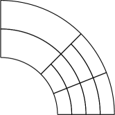
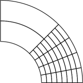
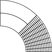
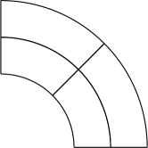
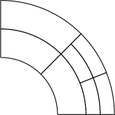
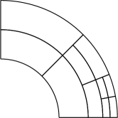
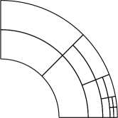
Figure 7. The domain $\Omega$ considered in Section 9 along with the initial mesh $\mathcal{T}_{0}$ and the first three refinements: in the right half of $\Omega$ (leading to arbitrary many hanging nodes) (top) and towards the point $(1,0)$ (violating the bounded patch overlap condition (84a)) (bottom).

We consider four different refinements of the initial mesh: 1) uniform refinement, where in each step, all elements in the parameter domain are bisected in both directions; 2) adaptive refinement, where in each step, a minimal set of elements $\mathcal{M}_{h}\subseteq\mathcal{T}_{h}$ is marked via the Dörfler marking

$$\theta\sum_{T\in\mathcal{T}_{h}}\big{(}\|\bm{\sigma}_{h}+\nabla u_{h}\|_{T}^{2}+\mathrm{osc}_{h}^{\rm rel}(T)^{2}\big{)}\leq\sum_{T\in\mathcal{M}_{h}}\big{(}\|\bm{\sigma}_{h}+\nabla u_{h}\|_{T}^{2}+\mathrm{osc}_{h}^{\rm rel}(T)^{2}\big{)}$$

with $\theta=0.5$ and subsequently refined via the refinement strategy from [GHP17] (see also Remark 8.7); 3) artificial refinement enforcing an arbitrary number of hanging nodes, where in each step, all elements in the parameter domain that are contained in $[0,1/2]\times[0,1]$ are bisected in both directions (see Figure 7, top); 4) artificial refinement enforcing an arbitrary number of overlapping patches $\omega_{\bm{a}}$, where in each step, the element in the parameter domain containing the point $(0,0)$, which is mapped onto $(1,0)$ under $\bm{F}$, is bisected in both directions (see Figure 7, bottom). In each case, new knots have multiplicity $m$.

The resulting effectivity indices $\frac{\|\bm{\sigma}_{h}+\nabla u_{h}\|_{\Omega}}{\|\nabla(u-u_{h})\|_{\Omega}}$ and $\frac{\|\bm{\sigma}_{h}+\nabla u_{h}\|_{\Omega}+\mathrm{osc}_{h}^{\rm rel}}{\|\nabla(u-u_{h})\|_{\Omega}}$ as function of the number of mesh elements $N$ in $\mathcal{T}_{h}$ are displayed in Figures 8–11. Recall from Propositions 8.4 and 8.6 that the efficiency constant in (84b) may theoretically depend on the space dimension $d$, the polynomial degree $\overline{p}$ (which itself depends on the considered smoothness, see Remark 6.10), $\max\{\|D\bm{F}\|_{\infty,\widehat{\Omega}},$ $\|(D\bm{F})^{-1}\|_{\infty,\widehat{\Omega}}\}$, and the overlap constant $C_{\rm over}$ from (84a) (which itself only depends on $\overline{p}$ for the first three refinements types, see Remark 8.7, but grows unboundedly in the fourth case). At least in this example, though, the dependence on $\overline{p}$ is not observed, and the equilibrated flux estimator $\|\bm{\sigma}_{h}+\nabla u_{h}\|_{\Omega}$ (plus oscillation terms) seems to be not only, as proven, robust with respect to the polynomial degrees $p$ and $\widetilde{p}$, but also with respect to the smoothness incarnated in $\overline{p}$. The increase of the effectivity indices on adaptively refined meshes with $\widetilde{p}=p+1$ in the right part of Figure 9 is only because of data oscillation, as we discuss below. Moreover, as theoretically shown in Proposition 8.6, we also numerically observe in Figure 10 the robustness with respect to the strength of the hierarchical refinement (number of hanging nodes). For the fourth refinement, (84a) is not uniformly satisfied, which, however, is again not reflected in the resulting efficiency constants. Note however that the computation of the equilibrated flux becomes very expensive in this case, as there are nodes ${\bm{a}}$ whose patches $\omega_{\bm{a}}$ coincide with the entire computational domain $\Omega$, so that the corresponding meshes $\mathcal{T}_{\bm{a}}$ are uniform refinements of $\mathcal{T}_{0}$ up to the same level as the element containing the point $(1,0)$. Additional numerical experiments were carried out for an exact solution $u(x,y)=\sin(2\pi x)\sin(2\pi y)$ on the square (not displayed), with similar results.

The “data oscillation” terms $\mathrm{osc}_{h}^{\rm rel}$ from (77b) are displayed separately in Figure 12, again as function of the number of mesh elements $N$ in $\mathcal{T}_{h}$. For the present smooth solution (85), one expects the error $\|\nabla(u-u_{h})\|_{\Omega}$ to decay as $\mathcal{O}(h^{p})\approx\mathcal{O}(N^{-p/2})$ for uniform mesh refinement. Recall from Remark 8.3 that $\mathrm{osc}_{h}^{\rm rel}$ are expected to decay in this case as $\mathcal{O}(h^{\widetilde{p}+2})$, i.e., as $\mathcal{O}(N^{-p/2-3/2})$ or $\mathcal{O}(N^{-p/2-2})$ for respectively $\widetilde{p}=p+1$ and $\widetilde{p}=p+2$. Figure 12 only concerns adaptive mesh refinement, where $\|\nabla(u-u_{h})\|_{\Omega}$ is still expected to decay as $\mathcal{O}(N^{-p/2})$. We do not have here theoretical indications for $\mathrm{osc}_{h}^{\rm rel}$, but we observe at least $\mathcal{O}(N^{-p/2})$ in most cases, even though the chosen $\widetilde{p}$ is theoretically inappropriate for higher smoothness as discussed above. For uniform mesh refinement (not displayed), we indeed observe $\mathcal{O}(h^{\widetilde{p}+2})$, following Remark 8.3.

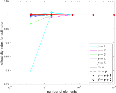
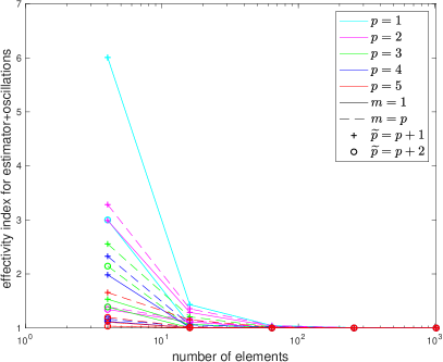
Figure 8. Effectivity indices $\frac{\|\bm{\sigma}_{h}+\nabla u_{h}\|_{\Omega}}{\|\nabla(u-u_{h})\|_{\Omega}}$ (left) and $\frac{\|\bm{\sigma}_{h}+\nabla u_{h}\|_{\Omega}+\mathrm{osc}_{h}^{\rm rel}}{\|\nabla(u-u_{h})\|_{\Omega}}$ (right) corresponding to the problem of Section 9 with uniform mesh refinement, polynomial degrees $p\in\{1,\dots,5\}$, multiplicities $m\in\{1,p\}$.

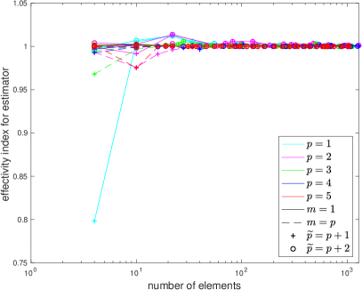
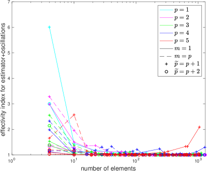
Figure 9. Effectivity indices $\frac{\|\bm{\sigma}_{h}+\nabla u_{h}\|_{\Omega}}{\|\nabla(u-u_{h})\|_{\Omega}}$ (left) and $\frac{\|\bm{\sigma}_{h}+\nabla u_{h}\|_{\Omega}+\mathrm{osc}_{h}^{\rm rel}}{\|\nabla(u-u_{h})\|_{\Omega}}$ (right) corresponding to the problem of Section 9 with adaptive mesh refinement, polynomial degrees $p\in\{1,\dots,5\}$, multiplicities $m\in\{1,p\}$.

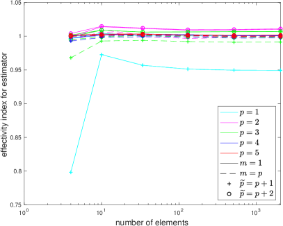
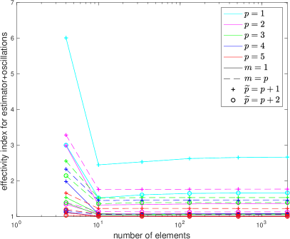
Figure 10. Effectivity indices $\frac{\|\bm{\sigma}_{h}+\nabla u_{h}\|_{\Omega}}{\|\nabla(u-u_{h})\|_{\Omega}}$ (left) and $\frac{\|\bm{\sigma}_{h}+\nabla u_{h}\|_{\Omega}+\mathrm{osc}_{h}^{\rm rel}}{\|\nabla(u-u_{h})\|_{\Omega}}$ (right) corresponding to the problem of Section 9 with artificial refinement enforcing a high number of hanging nodes (see Figure 7, top), polynomial degrees $p\in\{1,\dots,5\}$, multiplicities $m\in\{1,p\}$.

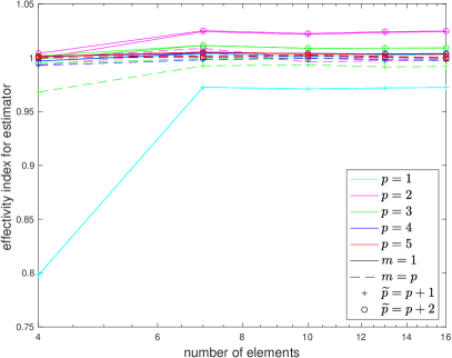
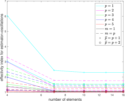
Figure 11. Effectivity indices $\frac{\|\bm{\sigma}_{h}+\nabla u_{h}\|_{\Omega}}{\|\nabla(u-u_{h})\|_{\Omega}}$ (left) and $\frac{\|\bm{\sigma}_{h}+\nabla u_{h}\|_{\Omega}+\mathrm{osc}_{h}^{\rm rel}}{\|\nabla(u-u_{h})\|_{\Omega}}$ (right) corresponding to the problem of Section 9 with artificial refinement enforcing a high number of overlapping patches (see Figure 7, bottom), polynomial degrees $p\in\{1,\dots,5\}$, multiplicities $m\in\{1,p\}$.

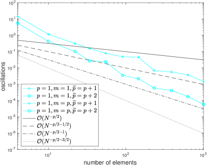
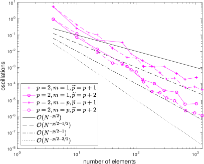
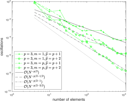
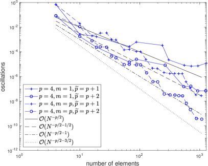
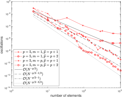
Figure 12. Oscillation terms $\mathrm{osc}_{h}^{\rm rel}$ from (77b) corresponding to the problem of Section 9 with adaptive mesh refinement, polynomial degrees $p\in\{1,\dots,5\}$, multiplicities $m\in\{1,p\}$.

Appendix A Proof of the broken polynomial extension property

In this section, we verify Assumption 6.8 for the spaces defined in Section 5.3. Recall the Piola transformations from (43) and (44)

$$\bm{\Phi}(\cdot):=\big{(}\det(D\bm{F})^{-1}(D\bm{F})(\cdot)\big{)}\circ\bm{F}^{-1}\quad\text{and}\quad\widetilde{\Phi}(\cdot):=\big{(}\det(D\bm{F})^{-1}(\cdot)\big{)}\circ\bm{F}^{-1}$$

and the identity (45)

$$\widetilde{\Phi}\big{(}\nabla{\cdot}(\cdot)\big{)}=\nabla{\cdot}\bm{\Phi}(\cdot);$$ (86)

see, e.g., [EG21, Lemma 9.6]. Following the imposition of the Neumann boundary condition in the space $\bm{H}_{0}(\mathrm{div},\omega_{\bm{b}})$ in (40), we denote by $\mathcal{F}_{\bm{b}}^{\rm N}$ the boundary faces of the local mesh $\mathcal{T}_{\bm{b}}$ if $\psi_{\bm{a}}\psi_{\bm{b}}\in H_{0}^{1}(\Omega)$ and such boundary faces of $\mathcal{T}_{\bm{b}}$ where $F\subset(\psi_{\bm{a}}\psi_{\bm{b}})^{-1}(\{0\})$ for $\psi_{\bm{a}}\psi_{\bm{b}}\not\in H_{0}^{1}(\Omega)$. By $\mathcal{F}_{\bm{b}}^{\rm int}$, we denote the interior faces of $\mathcal{T}_{\bm{b}}$. Analogously, we write $\widehat{\mathcal{F}}_{\bm{b}}^{\rm N}$ and $\widehat{\mathcal{F}}_{\bm{b}}^{\rm int}$ for the corresponding faces on the parameter mesh $\widehat{\mathcal{T}}_{\bm{b}}$. Finally, we write $\nabla_{\bm{b}}{\cdot}(\cdot)$ for the $\mathcal{T}_{\bm{b}}$- or $\widehat{\mathcal{T}}_{\bm{b}}$-piecewise divergence operator.

Since $\bm{\tau}_{h}\in\bm{RT}_{h}^{{\bm{a}},{\bm{b}}}=\bm{RT}^{\widetilde{\bm{p}}}(\mathcal{T}_{\bm{b}})$ and $\bm{V}_{h}^{{\bm{a}},{\bm{b}}}=\bm{RT}^{\widetilde{\bm{p}}}(\mathcal{T}_{\bm{b}})\cap\bm{H}_{0}(\mathrm{div},\omega_{\bm{b}})$ by (49), we can substitute in (58) $\bm{v}_{h}+\bm{\tau}_{h}=\bm{w}_{h}$ with $\bm{w}_{h}=\bm{\Phi}(\widehat{\bm{w}}_{h})$ and $\widehat{\bm{w}}_{h}\in\bm{RT}^{\widetilde{\bm{p}}}(\widehat{\mathcal{T}}_{\bm{b}})$, also using (50). This shows that

$$\min_{\begin{subarray}{c}\bm{v}_{h}\in\bm{V}_{h}^{{\bm{a}},{\bm{b}}}\\ \nabla{\cdot}\bm{v}_{h}=g_{h}\end{subarray}}\|\bm{v}_{h}+\bm{\tau}_{h}\|_{\omega_{\bm{b}}}=\!\!\!\min_{\begin{subarray}{c}\bm{w}_{h}\in\bm{RT}^{\widetilde{\bm{p}}}(\mathcal{T}_{\bm{b}})\\ \bm{w}_{h}{\cdot}\bm{n}_{\omega_{\bm{b}}}|_{F}=\bm{\tau}_{h}{\cdot}\bm{n}_{\omega_{\bm{b}}}|_{F}=:r_{F}\,\,\,\forall F\in\mathcal{F}_{\bm{b}}^{\rm N}\\ [\bm{w}_{h}{\cdot}\bm{n}_{\omega_{\bm{b}}}]_{F}=[\bm{\tau}_{h}{\cdot}\bm{n}_{\omega_{\bm{b}}}]_{F}=:r_{F}\,\,\,\forall F\in\mathcal{F}_{\bm{b}}^{\rm int}\\ \nabla_{\bm{b}}{\cdot}\bm{w}_{h}|_{T}=(g_{h}+\nabla_{\bm{b}}{\cdot}\bm{\tau}_{h})|_{T}=:r_{T}\,\,\,\forall T\in\mathcal{T}_{\bm{b}}\end{subarray}}\!\!\!\|\bm{w}_{h}\|_{\omega_{\bm{b}}}=\!\!\!\min_{\begin{subarray}{c}\widehat{\bm{w}}_{h}\in\bm{RT}^{\widetilde{\bm{p}}}(\widehat{\mathcal{T}}_{\bm{b}})\\ \bm{\Phi}(\widehat{\bm{w}}_{h}){\cdot}\bm{n}_{\omega_{\bm{b}}}|_{F}=r_{F}\,\,\,\forall F\in\mathcal{F}_{\bm{b}}^{\rm N}\\ [\bm{\Phi}(\widehat{\bm{w}}_{h}){\cdot}\bm{n}_{\omega_{\bm{b}}}]_{F}=r_{F}\,\,\,\forall F\in\mathcal{F}_{\bm{b}}^{\rm int}\\ \nabla_{\bm{b}}{\cdot}\bm{\Phi}(\widehat{\bm{w}}_{h})|_{T}=r_{T}\,\,\,\forall T\in\mathcal{T}_{\bm{b}}\end{subarray}}\!\!\!\|\bm{\Phi}(\widehat{\bm{w}}_{h})\|_{\omega_{\bm{b}}}.$$ (87)

With $\bm{n}_{\widehat{\omega}_{\bm{b}}}$ denoting the outer normal vector on $\partial\widehat{\omega}_{\bm{b}}$, elementary analysis, cf. [EG21, Lemma 9.11], provides the relation

$$(D\bm{F}^{\top}\circ\bm{F}^{-1})\,\bm{n}_{\omega_{\bm{b}}}=\bm{n}_{\widehat{\omega}_{\bm{b}}}\circ\bm{F}^{-1}|(D\bm{F}^{\top}\circ\bm{F}^{-1})\,\bm{n}_{\omega_{\bm{b}}}|$$

and thus

$$\bm{\Phi}(\widehat{\bm{w}}_{h}){\cdot}\bm{n}_{\omega_{\bm{b}}} =\Big{(}\big{(}\det(D\bm{F})^{-1}\widehat{\bm{w}}_{h}^{\top}(D\bm{F})^{\top}\big{)}\circ\bm{F}^{-1}\Big{)}\bm{n}_{\omega_{\bm{b}}}$$

$$=\Big{(}\widehat{\bm{w}}_{h}{\cdot}\bm{n}_{\widehat{\omega}_{\bm{b}}}\,\frac{|(D\bm{F}^{\top}\circ\bm{F}^{-1})\,\bm{n}_{\omega_{\bm{b}}}|}{\det(D\bm{F})}\Big{)}\circ\bm{F}^{-1}.$$

Hence, with $\widehat{F}:=\bm{F}^{-1}(F)$ and $\widehat{\bm{\tau}}_{h}:=\bm{\Phi}^{-1}(\bm{\tau}_{h})$, the first equation in the last minimum of (87) is equivalent to $\widehat{\bm{w}}_{h}{\cdot}\bm{n}_{\widehat{\omega}_{\bm{b}}}|_{\widehat{F}}=\widehat{\bm{\tau}}_{h}{\cdot}\bm{n}_{\widehat{\omega}_{\bm{b}}}|_{\widehat{F}}=:r_{\widehat{F}}$, and the second equation is equivalent to $[\widehat{\bm{w}}_{h}{\cdot}\bm{n}_{\widehat{\omega}_{\bm{b}}}]|_{\widehat{F}}=[\widehat{\bm{\tau}}_{h}{\cdot}\bm{n}_{\widehat{\omega}_{\bm{b}}}]_{\widehat{F}}=:r_{\widehat{F}}$. The identity (86) shows that the third equation is equivalent to $\nabla_{{\bm{b}}}{\cdot}\widehat{\bm{w}}_{h}|_{\widehat{T}}=\widetilde{\Phi}^{-1}(g_{h}+\nabla_{{\bm{b}}}{\cdot}\bm{\tau}_{h})=:r_{\widehat{T}}$. As $\|\bm{\Phi}(\widehat{\bm{w}}_{h})\|_{\omega_{\bm{b}}}\lesssim\|\widehat{\bm{w}}_{h}\|_{\widehat{\omega}_{\bm{b}}}$ (with a hidden constant depending only on $\|D\bm{F}\|_{\infty,\widehat{\Omega}}$), we can formulate (87) in the parameter domain

$$\min_{\begin{subarray}{c}\bm{v}_{h}\in\bm{V}_{h}^{{\bm{a}},{\bm{b}}}\\ \nabla{\cdot}\bm{v}_{h}=g_{h}\end{subarray}}\|\bm{v}_{h}+\bm{\tau}_{h}\|_{\omega_{\bm{b}}}\lesssim\min_{\begin{subarray}{c}\widehat{\bm{w}}_{h}\in\bm{RT}^{\widetilde{\bm{p}}}(\widehat{\mathcal{T}}_{\bm{b}})\\ \widehat{\bm{w}}_{h}{\cdot}\bm{n}_{\widehat{\omega}_{\bm{b}}}|_{\widehat{F}}=r_{\widehat{F}}\,\,\,\forall\widehat{F}\in\widehat{\mathcal{F}}_{\bm{b}}^{\rm N}\\ [\widehat{\bm{w}}_{h}{\cdot}\bm{n}_{\widehat{\omega}_{\bm{b}}}]_{\widehat{F}}=r_{\widehat{F}}\,\,\,\forall\widehat{F}\in\widehat{\mathcal{F}}_{\bm{b}}^{\rm int}\\ \nabla_{{\bm{b}}}{\cdot}\widehat{\bm{w}}_{h}|_{\widehat{T}}=r_{\widehat{T}}\,\,\,\forall\widehat{T}\in\widehat{\mathcal{T}}_{\bm{b}}\end{subarray}}\|\widehat{\bm{w}}_{h}\|_{\widehat{\omega}_{\bm{b}}}.$$ (88)

Finally, an application of [BPS09, Theorems 5 and 7] in two space dimensions or a similar procedure relying on [CDD08] in three space dimensions, see also [EV20, Theorem 2.5 and Corollary 3.3] building on [CM10, DGS12], yields that

$$\min_{\begin{subarray}{c}\widehat{\bm{w}}_{h}\in\bm{RT}^{\widetilde{\bm{p}}}(\widehat{\mathcal{T}}_{\bm{b}})\\ \widehat{\bm{w}}_{h}{\cdot}\bm{n}_{\widehat{\omega}_{\bm{b}}}|_{\widehat{F}}=r_{\widehat{F}}\,\,\,\forall\widehat{F}\in\widehat{\mathcal{F}}_{\bm{b}}^{\rm N}\\ [\widehat{\bm{w}}_{h}{\cdot}\bm{n}_{\widehat{\omega}_{\bm{b}}}]_{\widehat{F}}=r_{\widehat{F}}\,\,\,\forall\widehat{F}\in\widehat{\mathcal{F}}_{\bm{b}}^{\rm int}\\ \nabla_{{\bm{b}}}{\cdot}\widehat{\bm{w}}_{h}|_{\widehat{T}}=r_{\widehat{T}}\,\,\,\forall\widehat{T}\in\widehat{\mathcal{T}}_{\bm{b}}\end{subarray}}\|\widehat{\bm{w}}_{h}\|_{\widehat{\omega}_{\bm{b}}}\leq C_{\rm st}\min_{\begin{subarray}{c}\widehat{\bm{w}}\in\bm{H}(\mathrm{div},\widehat{\mathcal{T}}_{\bm{b}})\\ \widehat{\bm{w}}{\cdot}\bm{n}_{\widehat{\omega}_{\bm{b}}}|_{\widehat{F}}=r_{\widehat{F}}\,\,\,\forall\widehat{F}\in\widehat{\mathcal{F}}_{\bm{b}}^{\rm N}\\ [\widehat{\bm{w}}{\cdot}\bm{n}_{\widehat{\omega}_{\bm{b}}}]_{\widehat{F}}=r_{\widehat{F}}\,\,\,\forall\widehat{F}\in\widehat{\mathcal{F}}_{\bm{b}}^{\rm int}\\ \nabla_{{\bm{b}}}{\cdot}\widehat{\bm{w}}|_{\widehat{T}}=r_{\widehat{T}}\,\,\,\forall\widehat{T}\in\widehat{\mathcal{T}}_{\bm{b}}\end{subarray}}\|\widehat{\bm{w}}\|_{\widehat{\omega}_{\bm{b}}},$$

for a generic constant $C_{\rm st}$ only depending on the shapes of the elements in $\widehat{\mathcal{T}}_{{\rm uni}(0)}$. Here, $\bm{H}(\mathrm{div},\widehat{\mathcal{T}}_{\bm{b}})$ is the space of $\widehat{\mathcal{T}}_{\bm{b}}$-piecewise $\bm{H}(\mathrm{div})$-functions on $\widehat{\omega}_{\bm{b}}$, with the normal component understood as in [EV20, equation (2.6)]. The required compatibility condition

$$\sum_{\widehat{T}\in\widehat{\mathcal{T}}_{\bm{b}}}(r_{\widehat{T}}\,,\,1)_{\widehat{T}}-\sum_{\widehat{F}\in\widehat{\mathcal{F}}_{\bm{b}}^{\rm N}\cup\widehat{\mathcal{F}}_{\bm{b}}^{\rm int}}(r_{\widehat{F}}\,,\,1)_{\widehat{F}}=0$$

in case of $\psi_{\bm{a}}\psi_{\bm{b}}\in H_{0}^{1}(\Omega)$ follows from the assumption that $g_{h}$, and thus $\widetilde{\Phi}^{-1}(g_{h})$, has integral mean zero then. Finally,

$$\min_{\begin{subarray}{c}\widehat{\bm{w}}\in\bm{H}(\mathrm{div},\widehat{\mathcal{T}}_{\bm{b}})\\ \widehat{\bm{w}}{\cdot}\bm{n}_{\widehat{\omega}_{\bm{b}}}|_{\widehat{F}}=r_{\widehat{F}}\,\,\,\forall\widehat{F}\in\widehat{\mathcal{F}}_{\bm{b}}^{\rm N}\\ [\widehat{\bm{w}}{\cdot}\bm{n}_{\widehat{\omega}_{\bm{b}}}]_{\widehat{F}}=r_{\widehat{F}}\,\,\,\forall\widehat{F}\in\widehat{\mathcal{F}}_{\bm{b}}^{\rm int}\\ \nabla_{{\bm{b}}}{\cdot}\widehat{\bm{w}}|_{\widehat{T}}=r_{\widehat{T}}\,\,\,\forall\widehat{T}\in\widehat{\mathcal{T}}_{\bm{b}}\end{subarray}}\|\widehat{\bm{w}}\|_{\widehat{\omega}_{\bm{b}}}\lesssim\min_{\begin{subarray}{c}\bm{v}\in\bm{H}_{0}(\mathrm{div},\omega_{\bm{b}})\\ \nabla{\cdot}\bm{v}=g_{h}\end{subarray}}\|\bm{v}+\bm{\tau}_{h}\|_{\omega_{\bm{b}}}$$

with a hidden constant depending only on $\|(D\bm{F})^{-1}\|_{\infty,\widehat{\Omega}}$, as in (87) and (88). This concludes the proof.

References

- [AO00] Mark Ainsworth and J. Tinsley Oden. A posteriori error estimation in finite element analysis. Pure and Applied Mathematics (New York). Wiley-Interscience [John Wiley & Sons], New York, 2000.
- [BBdVC+06] Yuri Bazilevs, Lourenco Beirão da Veiga, J. Austin Cottrell, Thomas J. R. Hughes, and Giancarlo Sangalli. Isogeometric analysis: approximation, stability and error estimates for -refined meshes. Math. Models Methods Appl. Sci., 16(07):1031–1090, 2006.
- [BBF13] Daniele Boffi, Franco Brezzi, and Michel Fortin. Mixed finite element methods and applications, volume 44 of Springer Series in Computational Mathematics. Springer, Heidelberg, 2013.
- [BdVBSV13] Lourenco Beirão da Veiga, Annalisa Buffa, Giancarlo Sangalli, and Rafael Vázquez. Analysis-suitable T-splines of arbitrary degree: definition, linear independence and approximation properties. Math. Models Methods Appl. Sci., 23(11):1979–2003, 2013.
- [BdVBSV14] Lourenço Beirão da Veiga, Annalisa Buffa, Giancarlo Sangalli, and Rafael Vázquez. Mathematical analysis of variational isogeometric methods. Acta Numer., 23:157–287, 2014.
- [BG16a] Annalisa Buffa and Eduardo M. Garau. Refinable spaces and local approximation estimates for hierarchical splines. IMA J. Numer. Anal., 37(3):1125–1149, 2016.
- [BG16b] Annalisa Buffa and Carlotta Giannelli. Adaptive isogeometric methods with hierarchical splines: error estimator and convergence. Math. Models Methods Appl. Sci., 26(01):1–25, 2016.
- [BG17] Annalisa Buffa and Carlotta Giannelli. Adaptive isogeometric methods with hierarchical splines: Optimality and convergence rates. Math. Models Methods Appl. Sci., 27(14):2781–2802, 2017.
- [BG18] Annalisa Buffa and Eduardo M. Garau. A posteriori error estimators for hierarchical B-spline discretizations. Math. Models Methods Appl. Sci., 28(8):1453–1480, 2018.
- [BGG+22] Annalisa Buffa, Gregor Gantner, Carlotta Giannelli, Dirk Praetorius, and Rafael Vázquez. Mathematical foundations of adaptive isogeometric analysis. Arch. Comput. Methods Eng., 29:4479–4555, 2022.
- [BGV18] Cesare Bracco, Carlotta Giannelli, and Rafael Vázquez. Refinement algorithms for adaptive isogeometric methods with hierarchical splines. Axioms, 7(3):43, 2018.
- [BMV20] Jan Blechta, Josef Málek, and Martin Vohralík. Localization of the norm for local a posteriori efficiency. IMA J. Numer. Anal., 40(2):914–950, 2020.
- [BPS09] Dietrich Braess, Veronika Pillwein, and Joachim Schöberl. Equilibrated residual error estimates are -robust. Comput. Methods Appl. Mech. Engrg., 198(13-14):1189–1197, 2009.
- [BS08] Dietrich Braess and Joachim Schöberl. Equilibrated residual error estimator for edge elements. Math. Comp., 77(262):651–672, 2008.
- [CDD08] M. Costabel, M. Dauge, and L. Demkowicz. Polynomial extension operators for , and -spaces on a cube. Math. Comp., 77(264):1967–1999, 2008.
- [CF00] Carsten Carstensen and Stefan A. Funken. Fully reliable localized error control in the FEM. SIAM J. Sci. Comput., 21(4):1465–1484, 1999/00.
- [CHB09] J. Austin Cottrell, Thomas J. R. Hughes, and Yuri Bazilevs. Isogeometric analysis: toward integration of CAD and FEA. John Wiley & Sons, New York, 2009.
- [CM10] Martin Costabel and Alan McIntosh. On Bogovskiĭ and regularized Poincaré integral operators for de Rham complexes on Lipschitz domains. Math. Z., 265(2):297–320, 2010.
- [dB86] Carl de Boor. B(asic)-spline basics. Technical report, Mathematics Research Center, University of Wisconsin-Madison, 1986.
- [dB01] Carl de Boor. A practical guide to splines. Springer, New York, 2001.
- [DEV16] Vít Dolejší, Alexandre Ern, and Martin Vohralík. -adaptation driven by polynomial-degree-robust a posteriori error estimates for elliptic problems. SIAM J. Sci. Comput., 38(5):A3220–A3246, 2016.
- [DGS12] Leszek Demkowicz, Jayadeep Gopalakrishnan, and Joachim Schöberl. Polynomial extension operators. Part III. Math. Comp., 81(279):1289–1326, 2012.
- [DLP13] Tor Dokken, Tom Lyche, and Kjell F. Pettersen. Polynomial splines over locally refined box-partitions. Comput. Aided Geom. Design, 30(3):331–356, 2013.
- [DM99] Philippe Destuynder and Brigitte Métivet. Explicit error bounds in a conforming finite element method. Math. Comp., 68(228):1379–1396, 1999.
- [EG21] Alexandre Ern and Jean-Luc Guermond. Finite Elements I. Approximation and Interpolation, volume 72 of Texts in Applied Mathematics. Springer International Publishing, Springer Nature Switzerland AG, 2021.
- [ESV17a] Alexandre Ern, Iain Smears, and Martin Vohralík. Discrete -robust -liftings and a posteriori estimates for elliptic problems with source terms. Calcolo, 54(3):1009–1025, 2017.
- [ESV17b] Alexandre Ern, Iain Smears, and Martin Vohralík. Guaranteed, locally space-time efficient, and polynomial-degree robust a posteriori error estimates for high-order discretizations of parabolic problems. SIAM J. Numer. Anal., 55(6):2811–2834, 2017.
- [ET99] Ivar Ekeland and Roger Témam. Convex analysis and variational problems, volume 28 of Classics in Applied Mathematics. Society for Industrial and Applied Mathematics (SIAM), Philadelphia, PA, english edition, 1999. Translated from the French.
- [EV15] Alexandre Ern and Martin Vohralík. Polynomial-degree-robust a posteriori estimates in a unified setting for conforming, nonconforming, discontinuous Galerkin, and mixed discretizations. SIAM J. Numer. Anal., 53(2):1058–1081, 2015.
- [EV20] Alexandre Ern and Martin Vohralík. Stable broken and polynomial extensions for polynomial-degree-robust potential and flux reconstruction in three space dimensions. Math. Comp., 89(322):551–594, 2020.
- [GHP17] Gregor Gantner, Daniel Haberlik, and Dirk Praetorius. Adaptive IGAFEM with optimal convergence rates: Hierarchical B-splines. Math. Models Methods Appl. Sci., 27(14):2631–2674, 2017.
- [GJS12] Carlotta Giannelli, Bert Jüttler, and Hendrik Speleers. THB-splines: The truncated basis for hierarchical splines. Comput. Aided Geom. Design, 29(7):485–498, 2012.
- [GP20] Gregor Gantner and Dirk Praetorius. Adaptive IGAFEM with optimal convergence rates: T-splines. Comput. Aided Geom. Design, 81:101906, 2020.
- [HCB05] Thomas J. R. Hughes, J. Austin Cottrell, and Yuri Bazilevs. Isogeometric analysis: CAD, finite elements, NURBS, exact geometry and mesh refinement. Comput. Methods Appl. Mech. Engrg., 194(39):4135–4195, 2005.
- [HKMP17] Paul Hennig, Markus Kästner, Philipp Morgenstern, and Daniel Peterseim. Adaptive mesh refinement strategies in isogeometric analysis—A computational comparison. Comput. Methods Appl. Mech. Engrg., 316:424–448, 2017.
- [JKD14] Kjetil A. Johannessen, Trond Kvamsdal, and Tor Dokken. Isogeometric analysis using LR B-splines. Comput. Methods Appl. Mech. Engrg., 269:471–514, 2014.
- [JRK15] Kjetil A. Johannessen, Filippo Remonato, and Trond Kvamsdal. On the similarities and differences between classical hierarchical, truncated hierarchical and LR B-splines. Comput. Methods Appl. Mech. Engrg., 291:64–101, 2015.
- [KT15a] Stefan K. Kleiss and Satyendra K. Tomar. Guaranteed and sharp a posteriori error estimates in isogeometric analysis. Comput. Math. Appl., 70(3):167–190, 2015.
- [KT15b] Stefan K. Kleiss and Satyendra K. Tomar. Two-sided robust and sharp a posteriori error estimates in isogeometric discretization of elliptic problems. In Isogeometric analysis and applications 2014, volume 107 of Lect. Notes Comput. Sci. Eng., pages 231–246. Springer, Cham, 2015.
- [LL83] P. Ladevèze and D. Leguillon. Error estimate procedure in the finite element method and applications. SIAM J. Numer. Anal., 20(3):485–509, 1983.
- [Mat18] S. Matculevich. Functional approach to the error control in adaptive IgA schemes for elliptic boundary value problems. J. Comput. Appl. Math., 344:394–423, 2018.
- [PS47] William Prager and John L. Synge. Approximations in elasticity based on the concept of function space. Quart. Appl. Math., 5:241–269, 1947.
- [PV22] Jan Papež and Martin Vohralík. Inexpensive guaranteed and efficient upper bounds on the algebraic error in finite element discretizations. Numer. Algorithms, 89:371–407, 2022.
- [Rep99] Sergey I. Repin. A posteriori error estimates for approximate solutions to variational problems with strongly convex functionals. J. Math. Sci., 97(4):4311–4328, 1999.
- [Rep00a] Sergey I. Repin. A posteriori error estimation for nonlinear variational problems by duality theory. J. Math. Sci., 99(1):927–935, 2000.
- [Rep00b] Sergey I. Repin. A posteriori error estimation for variational problems with uniformly convex functionals. Math. Comp., 69(230):481–500, 2000.
- [Rep08] Sergey Repin. A posteriori estimates for partial differential equations, volume 4 of Radon Series on Computational and Applied Mathematics. Walter de Gruyter GmbH & Co. KG, Berlin, 2008.
- [Sch07] Larry Schumaker. Spline functions: Basic theory. Cambridge University Press, Cambridge, 2007.
- [SLSH12] Michael A. Scott, Xin Li, Thomas W. Sederberg, and Thomas J. R. Hughes. Local refinement of analysis-suitable T-splines. Comput. Methods Appl. Mech. Engrg., 213:206–222, 2012.
- [SM16] Hendrik Speleers and Carla Manni. Effortless quasi-interpolation in hierarchical spaces. Numer. Math., 132(1):155–184, 2016.
- [SMPZ08] Joachim Schöberl, Jens M. Melenk, Clemens Pechstein, and Sabine Zaglmayr. Additive Schwarz preconditioning for -version triangular and tetrahedral finite elements. IMA J. Numer. Anal., 28(1):1–24, 2008.
- [SZBN03] Thomas W. Sederberg, Jianmin Zheng, Almaz Bakenov, and Ahmad Nasri. T-splines and T-NURCCs. ACM Trans. Graph., 22(3):477–484, 2003.
- [TCHM19] Hoang Phuong Thai, Ludovic Chamoin, and Cuong Ha-Minh. A posteriori error estimation for isogeometric analysis using the concept of constitutive relation error. Comput. Methods Appl. Mech. Engrg., 355:1062–1096, 2019.
- [Ver13] Rüdiger Verfürth. A posteriori error estimation techniques for finite element methods. Numerical Mathematics and Scientific Computation. Oxford University Press, Oxford, 2013.
- [VGJS11] Anh-Vu Vuong, Carlotta Giannelli, Bert Jüttler, and Bernd Simeon. A hierarchical approach to adaptive local refinement in isogeometric analysis. Comput. Methods Appl. Mech. Engrg., 200(49):3554–3567, 2011.
- [Voh05] Martin Vohralík. On the discrete Poincaré–Friedrichs inequalities for nonconforming approximations of the Sobolev space . Numer. Funct. Anal. Optim., 26(7-8):925–952, 2005.
- [VV12] Andreas Veeser and Rüdiger Verfürth. Poincaré constants for finite element stars. IMA J. Numer. Anal., 32(1):30–47, 2012.