Correlation between Alignment-Uniformity
and Performance of Dense Contrastive Representations

Abstract

Recently, dense contrastive learning has shown superior performance on dense prediction tasks compared to instance-level contrastive learning. Despite its supremacy, the properties of dense contrastive representations have not yet been carefully studied. Therefore, we analyze the theoretical ideas of dense contrastive learning using a standard CNN and straightforward feature matching scheme rather than propose a new complex method. Inspired by the analysis of the properties of instance-level contrastive representations through the lens of alignment and uniformity on the hypersphere, we employ and extend the same lens for the dense contrastive representations to analyze their underexplored properties. We discover the core principle in constructing a positive pair of dense features and empirically proved its validity. Also, we introduces a new scalar metric that summarizes the correlation between alignment-and-uniformity and downstream performance. Using this metric, we study various facets of densely learned contrastive representations such as how the correlation changes over single- and multi-object datasets or linear evaluation and dense prediction tasks. The source code is publicly available at: https://github.com/SuperSupermoon/DenseCL-analysis

1 Introduction

Instance-level CL (Contrastive Learning) with a single-object dataset (e.gImageNet (Deng et al., 2009)) (Chen et al., 2020; Caron et al., 2020; Misra and Maaten, 2020; He et al., 2020; Trinh et al., 2019; Caron et al., 2018) has shown to be highly effective for learning visual representations in a self-supervised manner. To understand the semantic structures and behavior of this method, a few recent studies (Wang and Isola, 2020; Chen et al., 2021) analyzed the latent space (e.gunit hypersphere) from the perspective of uniformity and alignment (closeness). Intuitively, it is effective to analyze from these two perspectives, since features of all classes can be linearly separated from the rest of the feature space if they are sufficiently well clustered.

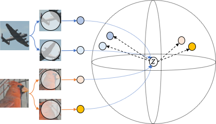
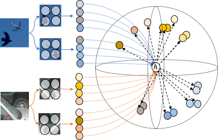
(a) Instance-level CL	(b) Dense CL

Figure 1: Contrastive Representations on the hypersphere. We demonstrate the difference in feature representation between instance- and dense CL on (a) single-object and (b) multi-object datasets. (a) represents an image as a single feature vector $\mathbf{z}\in\mathbf{R}^{d}$ containing global information, whereas (b) represents a set of vectors $\mathbf{h}\in\mathbf{R}^{d\times HW}$ exploited from a $H\times W$ feature map containing local feature information.

Although instance-level contrastive features have been successful in improving image classification performance, it has been observed that they do not enjoy the same transferability to dense prediction tasks (e.gobject detection tasks) (Wang et al., 2021; Xie et al., 2021; O Pinheiro et al., 2020; Wang et al., 2022; He et al., 2019; Yang et al., 2021; Caron et al., 2020; Chen et al., 2020). Since the receptive field of global averaged pooled features typically extends to the entire image, the pooled features are affected by background information, making it difficult to localize. To overcome this gap, recent studies (Wang et al., 2021; Xie et al., 2021; O Pinheiro et al., 2020; Wang et al., 2022) have developed dense CL with multi-object datasets (e.gMS-COCO (Lin et al., 2014)), using dense features to explicitly consider spatial information over regions and achieved comparable or better results compared to supervised ImageNet pre-training. Despite such initial success, these works beg an important yet unexplored question: "How different are the dense-level features compared to the instance-level features?" (Fig.1) In this work, we investigate the dense feature representation in terms of alignment and uniformity inspired by the pioneering analyses of (Wang and Isola, 2020; Chen et al., 2021). We extend the conventional contrastive loss (InfoNCE (Oord et al., 2018)) to construct a more principled dense-level contrastive loss, and introduce a scalar metric to succinctly report the alignment-uniformity behavior of latent features. Based on extensive experiments and analysis using both single and multi-object pre-training datasets, and instance-level (i.e. linear evaluation) and dense downstream task (i.e. object detection), our findings and contributions can be summarized as follows:

• We empirically show that the alignment-uniformity property in dense features is correlated with both instance-level and dense-level downstream task performance.

• We find that, contrary to our belief, instance-level contrastive features pre-trained on multi-object dataset can perform well on object detection, and dense contrastive features pre-trained on single-object dataset can perform well on linear evaluation, both cases following the alignment-uniformity principle.

• We discover the core principle in constructing a positive pair of dense features and empirically proved its validity with a simple index-wise matching.

2 Related work

After the advent of SimCLR (Chen et al., 2020), unsupervised CL (contrastive learning) was explosively researched on the instance-level (Caron et al., 2020; Misra and Maaten, 2020; He et al., 2020; Trinh et al., 2019; Caron et al., 2018). The core idea of this approach is sharing the InfoMax (Linsker, 1988) principle under instantiation by maximizing mutual information between two transformed versions of the same image (Tian et al., 2020a; Bachman et al., 2019; Wu et al., 2018). Recently Wang and Isola (2020) empirically proved that a unit $l2$-norm constrained contrastive loss (InfoNCE (Oord et al., 2018)) can be decomposed into a metric of alignment ($l2$-distance) and uniformity (average pairwise Gaussian potential). Also, they proved that optimizing contrastive loss is equivalent to optimizing the alignment between positive pairs and maintaining uniformity across all feature vectors in the hypersphere, and observed optimizing the alignment-uniformity properties is closely related to the downstream task performance such as linear evaluation. This hypersphere uniform distribution was generalized by Chen et al. (2021) and extended to a wider set of prior distributions (e.guniform hypercube or normal distribution). Our study is more related to Wang and Isola (2020), and we extend this analysis to dense features that contain local spatial information. Recently, He et al. (2019); Tan et al. (2020); Sun et al. (2019) demonstrate a transfer learning gap between instance-level pre-training and dense prediction tasks such as object detection. In an effort to overcome this gap, several works (Wang et al., 2021; Xie et al., 2021; O Pinheiro et al., 2020; Wang et al., 2022) generalized the instance discrimination from image-level to pixel-level to explore dense-level unsupervised CL and demonstrated improved downstream performance for dense prediction tasks. In contrast to numerous theoretical (Arora et al., 2019; Purushwalkam and Gupta, 2020b; Tian et al., 2020c; Tosh et al., 2021; Lee et al., 2021) and empirical analyses (Xiao et al., 2020; Robinson et al., 2021; Tian et al., 2020b; Zhao et al., 2020; Purushwalkam and Gupta, 2020a; Wang and Isola, 2020; Chen et al., 2021) to understand instance-level CL, no attempt has been made to understand dense CL. While there are many open questions, in this work we analyze how the pre-training impacts downstream tasks by extending the instance-level contrastive loss to the dense-level paradigm. Additionally, unlike instance-level CL where positive pairs are easily constructed via augmentations, constructing positive dense feature pairs in dense CL is non-trivial. Each of the previous works devised its own strategy to solve this problem, such as calculating the cosine similarity between dense features (Wang et al., 2021), attention-based set-wise matching (Wang et al., 2022), and matching dense features with associated regions (O Pinheiro et al., 2020; Xie et al., 2021). In this work, we take a more straightforward approach and adopt an index-wise matching between dense features from two augmented views. In the experiments section, we compare this rather simple strategy with more sophisticated ones such as using cosine similarity or optimal transport, and report that our approach leads to comparable or better downstream performance. Furthermore, we analyze the effectiveness of the index-wise pairing strategy in terms of whether the pre-training dataset consists of single-object images or multi-object images.

3 Method

3.1 Preliminary: Instance-level Contrastive Loss

Instance-level CL can be seen as the lower bound of mutual information ($MI$) between a positive pair $x$ and $y$ Oord et al. (2018); Bachman et al. (2019); Wu et al. (2018). Given $MI(x,y)=H(x)\mathbin{-}H(x|y)$, the two right-hand side terms can be linked to the following two properties (Wang and Isola, 2020; Chen et al., 2021):

• Uniformity $H(x)$: Maximizing entropy leads to uniformly distributed latent vectors.

• Alignment $H(x|y)$: Minimizing conditional entropy given the positive pair of each item makes them be aligned in the latent space.

Note that the general form of contrastive loss is defined as follows,

$$L^{InsCont}\text{=}\mathbin{-}\frac{1}{\mathcal{N}}\sum_{i,j\overset{\mathrm{i.i.d}}{\sim}\mathcal{B}}\log\frac{e^{sim(\mathbf{z}_{i},\mathbf{z}_{j})/\lambda}}{\sum_{k\overset{\mathrm{i.i.d}}{\sim}2\mathcal{N}}\mathbbm{1}_{[k\neq i]}e^{sim(\mathbf{z}_{i},\mathbf{z}_{k})/\lambda}},\quad sim(\mathbf{x},\mathbf{y})\text{=}\frac{\mathbf{x}\cdot\mathbf{y}}{\lVert\mathbf{x}\rVert\lVert\mathbf{y}\rVert}$$ (1)

where $\mathcal{N}$ denotes the number of randomly drawn instances, $\mathcal{B}$ the minibatch, $\mathbf{z}_{i}$ and $\mathbf{z}_{j}$ the positive pair of instance-level latent vectors projected into a hypersphere, $\lambda$ the temperature, and $\mathbbm{1}_{[k\neq i]\in{0,1}}$ an indicator function. Eq. (1) can be rewritten as follows by applying logarithmic rules:

where we confirm that the contrastive loss indeed consists of two objectives.

3.2 Dense Contrastive Loss

In order to analyze the behavior of dense features in CL, we first formalize the dense CL objective, a natural extension of instance-level CL to the dense-level. Let $f$ be a CNN encoder that transforms an input image $x$ to dense feature vectors $\mathbf{h}=f(x)=\{\mathbf{h}_{1},\mathbf{h}_{2},\ldots,\mathbf{h}_{HW}\},\enskip\mathbf{h}_{i}\in\mathbb{R}^{d}$, where ${HW}$ is the spatial dimension size.

Following the principle of $MI$ maximization in Eq. (1), we assume that all $\mathbf{h}_{i}$’s in a single image are $i.i.d$. Although $\mathbf{h}_{i}$’s do share some global information, this assumption is based on the fact that the values of each $\mathbf{h}_{i}$ are not identical because each contains different spatial information. Also, this assumption is often implicitly seen in the previous dense CL studies to extract the corresponding feature. In particular, DenseCLWang et al. (2021) compares all individual cosine similarity scores of features and pulls the most similar pairs closer. Also, SetsimWang et al. (2022) matches the corresponding feature set by calculating the set similarity using the attention score of the individual features. Therefore, by following the implicit $i.i.d$ assumption of the latest studies above, we perform index-wise feature matching by assuming $i.i.d$ of the output feature to form positive and negative pairs.

Dense contrastive loss can be defined as follows:

$$L^{DenseCont}\text{=}\mathbin{-}\frac{1}{\mathcal{N}}\sum_{i,j\overset{\mathrm{i.i.d}}{\sim}\mathcal{B}}\frac{1}{HW}\sum_{p}^{HW}\log\frac{e^{sim(\mathbf{h}_{(i,p)},\mathbf{h}_{(j,p)})/\lambda}}{\sum_{k\overset{\mathrm{i.i.d}}{\sim}2\mathcal{N}}\sum_{q}^{HW}\mathbbm{1}_{[k\neq i]\times[{\frac{q\neq p}{k\text{=}j}}]}e^{sim(\mathbf{h}_{(i,p)},\mathbf{h}_{(k,q)})/\lambda}},\quad sim(\mathbf{x},\mathbf{y})=\frac{\mathbf{x}\cdot\mathbf{y}}{\lVert\mathbf{x}\rVert\lVert\mathbf{y}\rVert}$$ (2)

where $\mathbf{h}_{(i,p)}$ indicates $p$-th dense feature of the $i$-th sample, and $\mathbbm{1}_{[k\neq i]\times[{\frac{q\neq p}{k\text{=}j}}]\in{0,1}}$ an indicator function. Note that a positive pair of dense features in our formulation consists of two dense features from the same index (i.e. spatial position) of each augmented image pair (see the numerator of Eq. (2)). We discuss the strategy for choosing positive and negative dense pairs in further detail in Section 3.3. Eq. (2) can also be rewritten as follows by applying logarithmic rules:

where we again observe that dense CL consists of alignment and distribution objectives. Therefore, by optimizing Eq. (2), dense features will asymptotically achieve the alignment-uniformity properties, similar to the instance-level CL.

To control these properties more directly, we adopt the metrics proposed in Wang and Isola (2020) and extend them to the dense-level. For the uniformity loss, we utilized a Gaussian potential kernel $G:\mathcal{S}^{d}\times\mathcal{S}^{d}\rightarrow\mathbb{R}_{+}$ (Wang and Isola, 2020; Borodachov et al., 2019; Cohn and Kumar, 2007) and the logarithm of the dense average pairwise Gaussian potential. Dense-level alignment-and-uniformity loss can be defined as:

$$L_{a}\triangleq\mathbin{-}\frac{1}{\mathcal{N}}\sum_{i,j\overset{\mathrm{i.i.d}}{\sim}\mathcal{B}}\frac{1}{HW}\sum_{p}^{HW}sim(\mathbf{h}_{(i,p)},\mathbf{h}_{(j,p)}),\quad L_{u}\triangleq log\frac{1}{\mathcal{N}}\sum_{i,j\overset{\mathrm{i.i.d}}{\sim}\mathcal{B}}\frac{1}{HW}\sum_{p}^{HW}G(\mathbf{h}_{(i,p)},\mathbf{h}_{(j,p)})$$

where $G(\mathbf{x},\mathbf{y})=e^{-{\lVert\mathbf{x}-\mathbf{y}\rVert}^{2}_{2}}$. denotes a pairwise Gaussian potential.

Perfect optimization of both properties is difficult to attain from a finite number of data points (Wang and Isola, 2020) but can be approximated when the data points (e.gminibatch) are sufficiently large. Therefore, in addition to Eq. (2), we also use $L_{a}$ and $L_{u}$ as the objective functions of the pre-training phase and observe whether the two properties are correlated with the downstream tasks for a wide range of scenarios.

3.3 Dense Feature Matching

One issue in dense CL is finding the appropriate features to form positive pairs. The key to matching dense features is that positive pairs must share information (i.e. alignment), while negative pairs must repel each other (i.e. uniformity). Many studies provide complex strategies to pair strong positives and negative pairs to the anchor $e.g.$ exploit geometrically identical features (Xie et al., 2021; O Pinheiro et al., 2020), calculate attention score (Wang et al., 2022), or use momentum queue to enlarge the size of negative samples (Wang et al., 2021). We address this issue with a spatially grounded dense feature matching (i.e. index-wise matching) based on the assumption from Section 3.2 that dense features of an instance and sampled data points are $i.i.d$. Our motivation for doing index-wise matching is to fairly compare the behavior of dense CL on multiple criteria as these tricks could yield various effects for each experiment.

Traditional CL (Chen et al., 2020; Caron et al., 2020; Misra and Maaten, 2020; He et al., 2020; Trinh et al., 2019; Caron et al., 2018) can learn feature representations when the distance between positive samples is shorter than between negative samples. Also, this approach admits that negative samples contain noisy samples of the positive class, and these noises are negligible when the strong negative samples are large enough. In this context, our simple approach is also reasonable and effective in learning feature representation. For two dense feature sets $\mathbf{h}_{1}=\{\mathbf{h}_{(1,1)},\ldots,\mathbf{h}_{(1,HW)}\},\enskip\mathbf{h}_{(1,i)}\in\mathbb{R}^{d}$ and $\mathbf{h}_{2}=\{\mathbf{h}_{(2,1)},\ldots,\mathbf{h}_{(2,HW)}\},\enskip\mathbf{h}_{(2,i)}\in\mathbb{R}^{d}$ from two augmented images, positive pairs are formed by vectors of the same index in each set $pos=\{(\mathbf{h}_{(1,i)},\mathbf{h}_{(2,i)}),\dots,(\mathbf{h}_{(1,HW)},\mathbf{h}_{(2,HW)})\}$ and the vectors of different indices $neg=\tilde{\mathbf{h}}_{2}\,\text{=}\,\{\mathbf{h}_{(2,j)},\ldots,\mathbf{h}_{(2,HW)}\},wherej\neq i$ are formed as negative pairs including other dense feature vectors from different data points in $\mathcal{B}$. Therefore, our matching strategy forms a soft positive pair while forming many strong negative pairs ($\approx$ 12.5k dense features of other images; features from different data points) and some noisy negative pairs (different indices from the same data point). Such noisy pairs in negative pairs can be ignored given a large number of strong negative pairs. Although some negative pairs could share information (e.g. $\mathbf{h}_{(1,i)}$ and $\mathbf{h}_{(2,i+1)}$), asymptotically all negative pairs should follow a uniform distribution. Surprisingly, this simple matching strategy showed successful performance in all our experiments, suggesting that our $i.i.d$ assumption was not unreasonable. We further investigate more sophisticated matching strategies that do not make such assumptions: dense feature matching based on cosine similarity (Wang et al., 2021), and set-wise matching based on earth mover distance (Wang et al., 2022). We report in the supplementary that both strategies show either similar or inferior performance to the simple index-wise matching.

4 Experiments

Our experiments primarily focus on the correlation analysis between feature representations after pre-training and the performance of downstream tasks: linear evaluation as the instance-level task and object detection as the dense-level task. We pose three questions regarding dense features: 1) How does the alignment-uniformity property of dense contrast learning correlate with the performance of object detection and linear evaluation? 2) How different is the behavior of dense feature representations on single or multi-object datasets? 3) How effective is the index-wise matching strategy in terms of different augmentation techniques?

In this section, we first describe experimental setup and how to quantify the correlation between alignment-uniformity property and downstream task performance. Then the following three subsections will address each of the three questions above.

4.1 Experimental Setup

Pre-training. We conduct pre-training experiments on two datasets: STL-10 (Coates et al., 2011) single-object dataset ($\sim$103k images from the training and unlabeled sets) and MS COCO (Lin et al., 2014) multi-object dataset($\sim$118k images from the training set). We closely follow the hyper-parameters and data augmentation rules from the official implementation of Wang and Isola (2020) for STL-10 and DenseCL (Wang et al., 2021) for COCO. We use Resnet18 as the backbone and extract the dense features from the penultimate layer (i.e. before the global average pooling layer). Then, these dense features are projected to two different sub-head blocks depending on the training scheme (instance-versus-dense). We train 200 STL-10 pre-trained models and 120 COCO pre-train models for 200 epochs with instance- and dense-level CL. Each model is optimized with a differently weighted combination of $L_{a}$ and $L_{u}$, or various values of the temperature $\tau$ of $L_{InfoNCE}$. Please refer to the supplementary for further details.

Instance-level Evaluation. To evaluate the instance-level linear separation ability, we employ the STL-10 linear evaluation. We freeze the pre-trained weights and fine-tune only one additional linear classification layer for 100 epochs, strictly following the settings of Wang and Isola (2020). We use these results as a reference to correlate the instance-level alignment-uniformity properties using the global average pooled feature for each instance.

Dense-level Evaluation. When evaluating dense features, we follow the standard object detection protocol using the Faster R-CNN (Ren et al., 2015) detector (R18-C4 backbone) on the PASCAL VOC trainval 07+12 set and testing on the VOC test 2007 set. Optimization takes a total of 24k iterations. The learning rate is initialized to 0.02 and decayed to be 10 times smaller after 18k and 22k iterations. We use average precision (AP) as an evaluation metric and analyze the correlation by measuring the alignment-uniformity properties of dense features.

Quantifying Correlation. We quantify the strength of the correlation between alignment-uniformity properties and downstream task performance by utilizing the scalar-valued
Kendall’s $\tau$, which is a rank-based correlation metric. Given $\mathcal{N}$ pre-trained models, the two losses ($L_{a}$, $L_{u}$), and the downstream task performance $P_{task}$ are reordered with min-max normalization across $\mathcal{N}$ models as $r(L_{a})$, $r(L_{u})$, and $r(P_{task})$. Kendall’s $\tau$ correlation metric is

$$\tau\text{=}\frac{P\mathbin{-}Q}{\sqrt{(P+Q+T)(P+Q+U)}}$$

where, $P$ and $Q$ are the numbers of ordered and disordered pairs in $\{r(L_{a_{i}})+r(L_{u_{i}}),r(P_{i})\},$ $i\in\mathcal{N}$. $T$ and $U$ are the numbers of ties in $\{r(L_{a_{i}})+r(L_{u_{i}})\}$ and $r(P_{i})$, respectively. The correlation value varies between -1 and +1, with a value close to 0 indicating a weak correlation. Note that a negative correlation between the losses ($\{r(L_{a_{i}})+r(L_{u_{i}})\}$) and downstream task performance ($P_{task}$) indicate that alignment-uniformity are desirable properties, and contrastive pre-training is useful.

4.2 Results of Pre-training on Single-object Dataset

Table 1: Single-object dataset results of instance and dense-level evaluation. We show the results for two different training scheme( $L_{InfoNCE}$ and $L_{a}\;\&\;L_{u}$) in a total of 200 experiments. $L_{a}\;\&\;L_{u}$ indicates loss of alignment and uniformity.

Pretraining	Loss	Instance-level Evaluation					Dense-level Evaluation
		linear evaluation(Acc)				correlation	object detection(AP)				correlation
		exp	max	Avg	top10	$\tau$	exp	max	Avg	top10	$\tau$
	$L_{a}\enskip\&\enskip L_{u}$	70	76.16	64.39	75.56	-0.50	70	40.37	37.21	40.14	-0.31
Instance	$L_{InfoNCE}$	30	75.47	71.99	74.97	-0.07	30	43.38	40.17	42.33	-0.41
	$total$	100	76.16	66.51	75.61	-0.45	100	43.38	38.02	42.33	-0.41
	$L_{a}\enskip\&\enskip L_{u}$	70	75.45	64.61	75.01	-0.19	70	43.44	38.99	43.19	-0.22
Dense	$L_{InfoNCE}$	30	75.12	60.85	74.18	-0.01	30	43.71	39.63	42.80	-0.54
	$total$	100	75.45	63.47	75.13	-0.32	100	43.71	39.2	43.31	-0.12
Random init		1	28.04	-	-	1	31.93	-	-

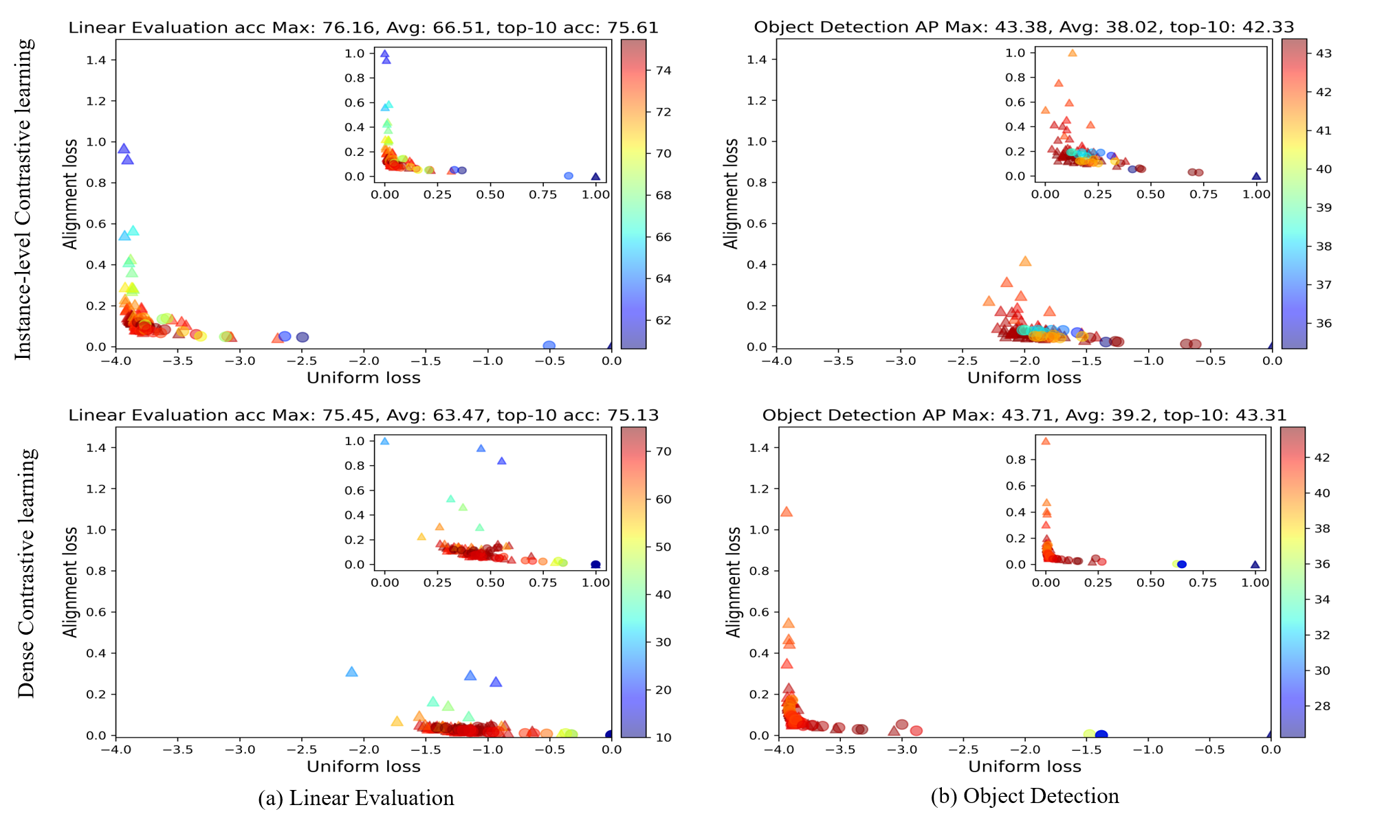
Figure 2: We show the alignment-uniformity property and downstream task performance for each 100 STL10 pre-trained models using instance- or dense-level features. All pre-trained models perform linear evaluation and object detection, then mark each point with color to show the performance. X and Y axes represent uniformity and alignment with a fixed scale. The symbol $\triangle$ and $\circ$ denotes $L_{InfoNCE}$ and $L_{a}\;\&\;L_{u}$, respectively. We also show normalized $L_{a}\;\&\;L_{u}$ values in the upper right corner. Note that we examine the alignment-uniformity properties using the features depending on the evaluation aspect (instance vs dense) regardless of the pre-training scheme.

Instance-level Evaluation. Wang and Isola (2020) demonstrated that the linear evaluation performance increased with the tendency to optimize alignment-uniformity. Inspired by its findings, we investigate the performance of linear evaluation and alignment-uniformity properties on the STL-10 testset using a global average pooling feature. As shown in Fig. 2 (a), the overall trend showed that the linear evaluation performance improved for the optimized alignment-uniformity property in both instance-level and dense CL, and all experiments showed a negative correlation (negative value of $\tau$ in Table 1). Also, instance-level and dense CL results achieved similar performance with a maximum accuracy of 76.16 and 75.45. These results show that dense contrast learning pre-trained on a single-object dataset has the ability to linearly separate by capturing the global information. We further investigate the behavior in the object detection task.

Dense-level Evaluation. To investigate the dense-level evaluation, we analyze the correlation between the alignment-uniformity of dense features on the STL-10 testset and VOC object detection performance. In this experiment, we can observe that the overall trend of the object detection performance is also correlated with the alignment-uniformity property in both instance-level and dense CL (Fig. 2 (b)) . Similar performance was achieved with a maximum AP of 43.38 and 43.71 in both instance-level and dense CL. The instance-level and dense CL using a single object showed a negative correlation between the alignment-uniformity and object detection ability with negative $\tau$ (Table 1). However, similar trends and performance may have been reached between instance level and dense contrast learning due to the inherent object-centric bias of the STL10 dataset. Still, the gap between the two pre-training schemes remains unknown. Therefore, we perform pre-training on a more complex setup involving multiple objects with the COCO dataset to ensure whether the correlation results of the STL10 pre-training are preserved.

4.3 Results of Pre-training on Multi-object Dataset.

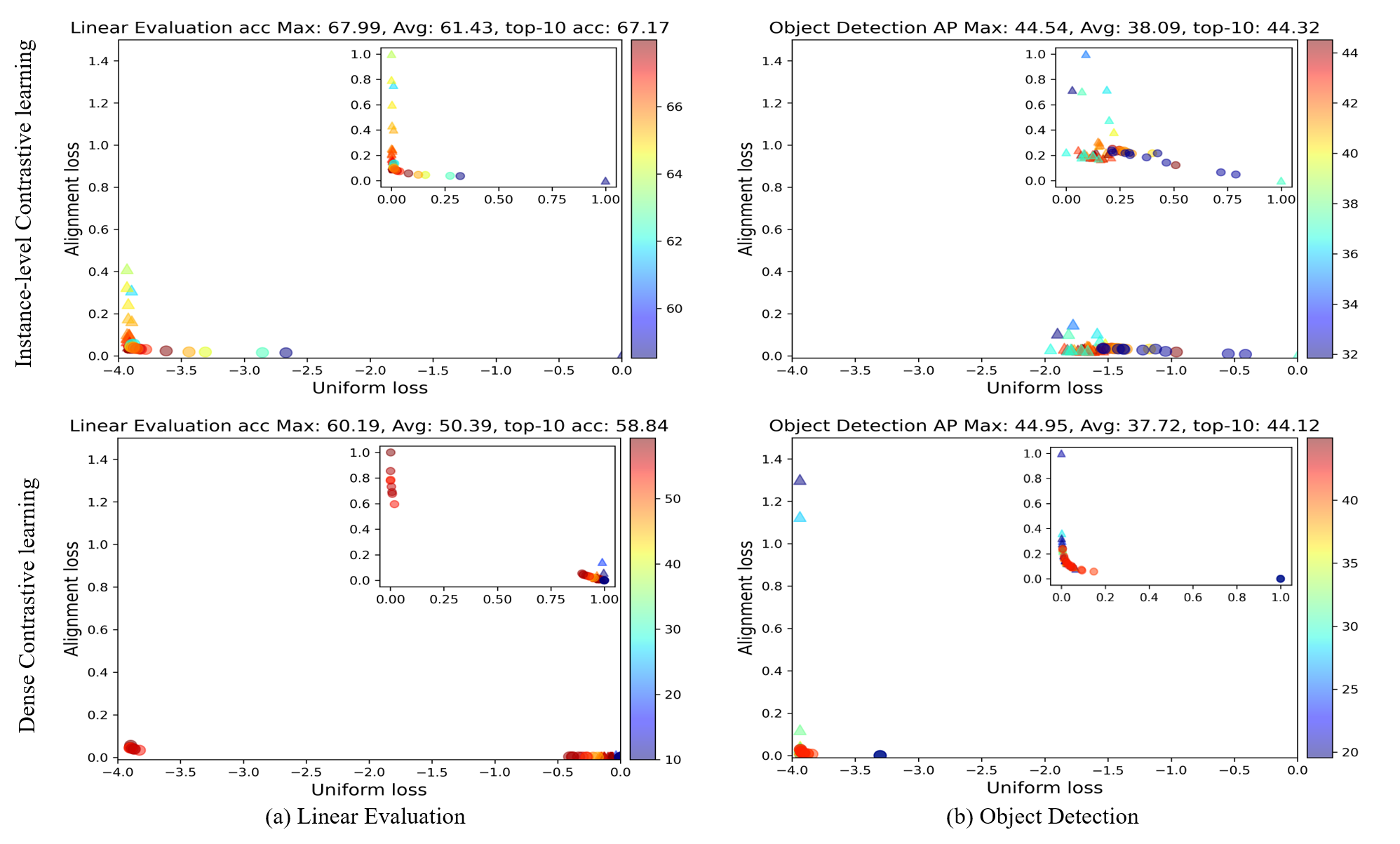
Figure 3: We show the alignment-uniformity property and downstream task performance for each 60 COCO pre-trained models using instance- or dense-level features. Each point is marked with color to show its performance and uniformity and alignment properties are represented in X and Y axes with a fixed scale. The symbol $\triangle$ and $\circ$ denotes $L_{InfoNCE}$ and $L_{a}\;\&\;L_{u}$, respectively.

Instance-level Evaluation. We conduct instance-level evaluations on COCO pre-trained models. The alignment-uniformity properties were measured using the global average pooled feature on the COCO testset while performing linear evaluation using the STL10 dataset. As shown in Fig. 3 (a), the trends of instance-level CL showed strong negative correlations with $\tau$ of -0.67 (Table 2). However, for the pre-training scheme with Dense CL, the results showed an irregular pattern depending on the uniformity, showing a weak correlation of -0.01 tau. Also, COCO pre-training showed inferior to STL pre-training in linear evaluation with maximum accuracy of 67.99 and 60.19 in instance-level and dense CL. We perform an object detection task to investigate whether such a performance gap occurs in dense prediction tasks.

Dense-level Evaluation. To evaluate the dense features on COCO pre-trained model, we analyze the correlation between alignment-uniformity of dense features on COCO testset and VOC object detection performance. As seen from Fig. 3 (b), all experiments showed high performance as the alignment-uniformity metric decreased. Also, the instance-level and dense CL showed high performance with maximum AP of 44.54 and 44.95 and $\tau$ of -0.21 and -0.13 Table 2. From these results, pre-training schemes with instance-level or dense-contrast learning using multiple objects perform well in dense prediction tasks despite the complexity of rich semantic information.

Table 2: Multi-object dataset results for instance and dense-level evaluation.

Pretraining	Loss	Instance-level Evaluation					Dense-level Evaluation
		linear evaluation(Acc)				correlation	object detection(AP)				correlation
		exp	max	Avg	top10	$\tau$	exp	max	Avg	top10	$\tau$
	$L_{a}\;\&\;L_{u}$	40	67.58	59.48	66.75	-0.54	40	44.54	38.27	43.94	-0.23
Instance	$L_{InfoNCE}$	20	67.99	65.05	66.63	-0.67	20	44.51	37.77	42.83	-0.03
	$total$	60	67.99	61.43	67.17	-0.67	60	44.54	38.09	44.32	-0.13
	$L_{a}\;\&\;L_{u}$	40	60.19	53.41	58.64	-0.21	40	44.71	36.99	42.90	-0.41
Dense	$L_{InfoNCE}$	20	59.29	46.36	57.30	-0.1	20	44.95	38.69	42.89	-0.54
	$total$	60	60.19	50.39	58.84	-0.01	60	44.95	37.72	44.12	-0.21
Random init		1	28.04	-	-	-	1	31.93	-	-	-

4.4 Confusing positive samples in Dense CL

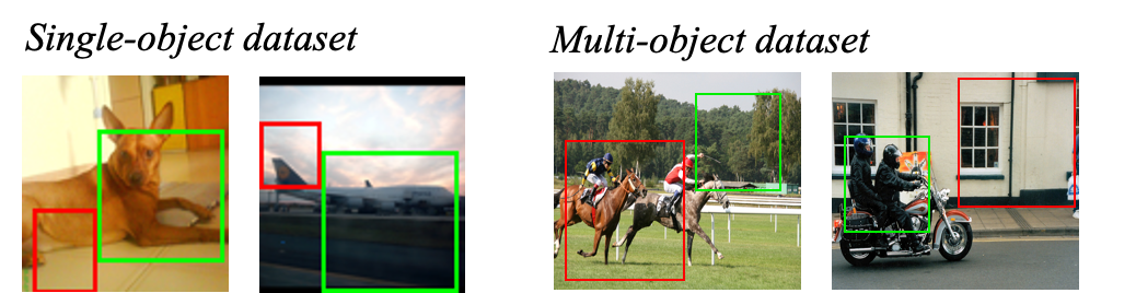
Figure 4: Confusing positive samples. The distances between the positive and negative pairs are similar.

Our assumption of feature matching by the index for positive pairs is that all features are $i.i.d.$, but two views from the same image should contain shared information. Single-object datasets, such as STL-10, are discriminated inter-class and object-centered. Due to the innate bias in these data sets, the mutual information in positive pairs (two random views in the same image) naturally shares similar information. However, in more complex setups with multiple objects, such as COCO, there is less chance of sharing semantically identical information even in positive pairs. To further investigate these biases in the data set, we analyze using non-overlapping image settings for confusing positive samples on STL10 and COCO datasets.

Table 3: Dense contrastive learning using not-obvious positive samples.

Pretraining		Instance-level Evaluation					Dense-level Evaluation
		linear evaluation(Acc)				correlation	object detection(AP)				correlation
		exp	max	Avg	top10	$\tau$	exp	max	Avg	top10	$\tau$
Single-object		46	69.94	57.60	68.74	-0.35	46	43.06	40.01	42.78	-0.65
Multi-object		12	54.89	40.30	44.80	-0.15	12	32.49	32.03	32.12	0.03
Random init		1	28.04	-	-	-	1	31.93	-	-	-

In Table 3, the STL10 pre-training results of the linear evaluation and object detection achieved high performance on a single object dataset and showed a strong negative correlation. However, pre-training with confusing positive samples on multi-object datasets showed inferior results in linear evaluation and object detection tasks. In particular, object detection showed similar performance with random initialization result (maximum AP of 31.93) in achieving the maximum AP of 32.49 in the object detection task. It showed a positive correlation with alignment-uniformity ($0.03\tau$). Therefore, the positive pairing method plays a crucial role in dense contrast learning so that positive pairs can share mutually agreeable information in multi-object datasets. Detailed setup and further experiments are shown in supplementary.

5 Conclusion

In this work, we mainly analyze the theoretical ideas of dense CL using a standard CNN and straightforward feature matching scheme rather than propose a new complex method. By extending existing instance-level CL analysis methods to dense-level, we observe the correlation between alignment-uniformity property of dense features and downstream tasks with newly proposed scalar metrics (linear evaluation and object detection). Also, we discover the core principle in constructing a positive pair of dense features and empirically proved its validity with a simple index-wise matching. In extensive experiments, we find that, regardless of pre-training schemes (instance-level or dense CL), pre-training on single object datasets showed the ability to linearly separate by capturing the global information and perform well on object detection tasks on multiple object datasets. Furthermore, our work can be potentially used to compare the performance of different CL schemes by evaluating alignment-uniformity properties of instance- and dense-level features before performing downstream tasks. The novelty of our work lies in carefully designed experiments and evaluation metric, allowing a reliable conversion from the “expected” to “confirmed”. We believe that the researchers can now safely rely on our findings and move on to developing more principled CL methods in the future, while treating our methods as a minimum baseline.

6 Supplementary

6.1 Experimental setup details

Architecture. We use Resnet18 as the backbone and extract the dense features from the penultimate layer. Then, these dense features (512-dim) are projected to two different sub-head blocks depending on the training scheme (instance-versus-dense). For the instance feature embedding, the projection head consists of a global pooling layer and the configuration of MLP(512-dim)-ReLU-MLP(128-dim). However, dense feature embedding removes the global pooling layer and replaces the MLP head with a 1 x 1 convolution layer to keep the spatial information: the configuration of Conv(512-dim)-ReLU-Conv(128-dim).

Pretraining setup. We conduct pretraining experiments following the data augmentation rule of Wang and Isola (2020) for STL10 pretraining: random horizontal flip, random color jittering, random grayscale conversion, and $64\times 64$ pixel crop with the scale 0.08 to 1.0 of the original image (an average 0.6 intersection ratio between two cropped images.) We use SGD as our optimizer with the learning rate decayed by a factor of 0.1 at epochs 155, 170, and 185. The SGD momentum is set to 0.9. For COCO pretraining, we follow Wang et al. (2021) to adopt data augmentation with random horizontal flip, random color jittering, random grayscale conversion, and $224\times 224$ pixel crop is taken with the scale 0.2 to 1.0 of the original image (an average 0.7 intersection ratio between two cropped image). We adopt SGD as the optimizer and set its weight decay and momentum to 0.0001 and 0.9 with a reciprocal learning rate decay schedule (warm-up iteration set to 0). All experiments are performed on 4-8 2080 Ti GPUs, RTX-3090 GPUs, and RTX-A6000 GPUs.

Evaluation protocol. We adopt augmentation rule to measure the alignment-uniformity property in stl10 and coco datasets:

• alignment: Random resized crop with the scale 0.95 to 1.0 of the original image, color jittering, and random grayscale conversion.

• uniformity: Resize and centercrop.

We measure the $L_{a}$ and $L_{u}$ properties for instance-level and density features. All features were $L2$-normalized, as the metrics are defined on the hypersphere. For instance-level evaluation, each instance is transformed to a global averaged pooled feature by $\mathbf{f}$ and then measured the alignment and uniformity properties in $\mathcal{B}$. For dense-level evaluation, each instance is transformed to a dense feature set by $\mathbf{f}$ and then measures the alignment and uniformity properties in $\mathcal{B}$. For linear evaluation details, we follow the standard linear evaluation on the STL10 protocol and report results on the validation set. We report performance after learning linear classifiers for 100 epochs, with an initial learning rate of 0.001, a batch size of 128, and a step learning rate schedule that drops at epochs 60 and 80 with the Adam optimizer.

6.2 Dense Feature Matching.

In our experiment, we assumes all dense features are $i.i.d.$. Namely, we consider a one-to-one relationship. To explore the one-to-many and many-to-many relationships, we investigate sophisticated matching strategies with $infoNCE$ loss ($L_{c}$): 1) one-to-many: dense feature matching based on cosine similarity Wang et al. (2021), and 2) many-to-many: set-wise matching based on earth mover distance.

6.2.1 One-to-Many Feature Matching

Inspired by the Wang et al. (2021), we perform maximum cosine similarity feature matching. As all our experimental settings are similar to SimCLR, we extract feature maps from a single encoder $\mathbf{f}$ and compute cosine similarity matching in $\mathcal{B}$. This setting considers a one-to-many relationship. Specifically, after two augmented views $x$ and $x^{\prime}$ are fed to $\mathbf{f}$ from the same input image, $\mathbf{h}_{1}=f(x)=\{\mathbf{h}_{1},\mathbf{h}_{2},\ldots,\mathbf{h}_{HW}\},\enskip\mathbf{h}_{i}\in\mathbb{R}^{d}$, and $\mathbf{h}_{2}=f(x^{\prime})=\{\mathbf{h}_{1},\mathbf{h}_{2},\ldots,\mathbf{h}_{HW}\},\enskip\mathbf{h}_{i}\in\mathbb{R}^{d}$ are acquired, where ${HW}$ is the spatial dimension size. Then, each dense feature of $\mathbf{h}_{1}$ retrieves the maximum cosine similarity value in $\mathbf{h}_{2}$ as a positive pair. Therefore, the number of positive pairs in each instance equals the number of dense features ($\mathbf{h}_{1}$). For negative pairs, $\mathbf{h}_{1}$ computes cosine similarity with the dense features of other instances in $\mathcal{B}$, pushing each other.

$$positive=argmax_{(i,j)}sim(\mathbf{h}_{(i,j)},\mathbf{h}_{(i,j)}),$$

$$neagtive=argmax_{(i,j)}\sum_{k\neq i}^{\mathcal{N}}sim(\mathbf{h}_{(i,j)},\mathbf{h}_{(k,j)}),$$

We train the models on the STL10 and COCO datasets and evaluate linear evaluation and object detection tasks. As suggested by DenseCL, we also pre-train the model with a weighting ratio of 0.5 for instance-level (global mean pooling) and dense features. We emphasize that both linear evaluation and object detection fail (Table 4 Cos with $L_{d}$) when using dense features as the only training vector for computing cosine similarity in the SimCLR setup. This shows that mode collapse occurs during pre-training and proves that cosine matching is a suboptimal method for dense feature mapping.

6.2.2 Many-to-Many Feature Matching

We show a many-to-many matching method of dense features. Set-wise dense feature matching is recently studied Wang et al. (2022) because the dense-level correspondence tends to be noisy because of many similar misleading features, e.gbackgrounds. We focus on this set-wise matching method and leverage earth mover distance ($i.e.$ optimal transport problem) for dense feature matching. Earth Mover’s Distance (EMD) Rubner et al. (2000); Wu et al. (2021) is a many-to-many matching method in which the individual element distances are constructed as the distances between two sets of distributions, the discrete form of which can be formulated as an optimal transport problem. Specially, for two feature maps $\mathbf{h}_{1}$, $\mathbf{h}_{2}$, EMD between two feature maps as the minimum transport cost from $\mathbf{h}_{1}$ to $\mathbf{h}_{2}$.

$$U(r,c)\textbf{=}\{P\in\mathbb{R}^{HW\times HW}|P\mathbbm{1}\textbf{=}\mathbf{r},P^{T}\mathbbm{1}\textbf{=}\mathbf{c}\}.$$

where, $\mathbbm{1}\in\mathbb{R}^{HW}$ are the vectors of all ones. $\mathbf{r}$ and $\mathbf{c}$ are marginal weights of matrix $P$ onto its rows and columns, respectively. Then, for the transport cost map ($\mathcal{TM}$), we utilized the cosine distance between $\mathbf{h}_{1}$ and $\mathbf{h}_{2}$. EMD is defined as follows:

$$EMD(r,c)\enskip\textbf{=}\enskip\min_{P\in U(r,c)}<P,\mathcal{TM}>$$

where, $\mathcal{TM}$ is the cosine distance matrix between $\mathbf{h}_{1}$ and $\mathbf{h}_{2}$ and <$\cdot$, $\cdot$> stands for the Frobenius dot-product between two matrices.

We calculate the optimal transport using a fast iterative solution named Sinkhorn-Knopp algorithm with a regularization term $E=0.1$ as:

$$\min_{P\in U(r,c)}<P,\mathcal{TM}>+\frac{1}{\lambda}E(P),$$

where $E(P)\textit{=}P(logP\mathrm{-}1)$ and $\lambda$ is a constant hyper-parameter that controls the intensity of regularization term. The approximated optimal transprot plan $P^{*}=diag(v)\times P\times diag(u)$, where $P=e^{-\lambda\mathcal{TM}}$ is the element-wise exponential of $-\lambda\mathcal{TM}$ and $v$ and $u$ are two vectors of scaling coefficients chosen so that the resulting matrix $P\in U(r,c)$. The vector $u$ and $v$ can be obtanied via a simple iteration as follows:

$$\forall i,\enskip v_{i}^{n+1} \leftarrow\frac{r_{i}}{\sum_{j}P_{i,j}u_{j}^{n}}$$

$$\forall j,\enskip u_{j}^{n+1} \leftarrow\frac{c_{j}}{\sum_{i}P_{i,j}v_{j}^{n+1}}$$

After iterate $N=10$ times, $P^{*}$ can be obtained. Finally, we can compute the similarity score $OT_{distance}$ between two dense features ($\mathbf{h}_{1}$ and $\mathbf{h}_{2}$) with:

$$OT_{distance}=<P,\mathcal{TM}>$$

Despite this complex matching process and computational overhead, we find that the STL10 and COCO pretraining obtained inferior results in the linear evaluation and comparable to our index-wise matching in object detection (Table 4). Therefore, we believe that index-wise matching method is straightforward and reasonable without additional computational overhead.

Table 4: Dense feature matching. $L_{i}$ and $L_{d}$ indicates instance-level and dense contrastive learning. $L_{i}$ + $L_{d}$ represent pre-training with weight ratios of 0.5 each. Cos and OT denote matching methods with cosine similarity and optimal transport. Cos (COCO) and OT (COCO) experiments used same hyperparameters with Wang et al. (2021). We show our index-wise matching (Ind) results.

		linear evaluation (Acc)				object detection (AP)
	Loss	exp	max	mean	top10	exp	max	mean	top10
Cos (STL10)	$L_{i}$ + $L_{d}$	20	11.92	10.2	10.4	20	43.68	41.34	42.68
Cos (STL10)	$L_{d}$	20	10	10	10	20	28.49	1.42	2.85
OT (STL10)	$L_{d}$	20	59.32	30.66	38.9	20	40.4	39.44	39.81
Cos (COCO)	$L_{i}$ + $L_{d}$	1	22.82	22.82	-	1	43.83	43.83	-
OT (COCO)	$L_{d}$	1	22.85	22.85	-	1	43.39	43.39	-
Ind (stl10)	$L_{d}$	100	75.45	63.47	75.13	100	43.71	39.2	43.31
Ind (coco)	$L_{d}$	60	60.19	50.39	58.84	60	44.95	37.72	44.12

6.3 Detailed Results.

We show the detailed pretraining phase and downstream task results. Specifically, we show the hyperparameter settings for batch size, learning rate, ratio of loss weights between $L_{a},L_{u},$ and $L_{c}$ during pretraining, and normalized temperature $\tau$ for $L_{c}$. In addition, each pre-trained model shows the results of Instance-level versus Dense-level evaluation (metrics for $L_{a},L_{u},$ and downstream task performance) according to two evaluation aspects. Table 5 shows 100 STL pretraining based on instace-level contrastive learning, Table 6 shows 100 STL pretraining based on dense contrastive learning. Also, Table 7 and Table 8 show 60 coco pretraining based on instace-level contrastive learning and 60 coco pretraining based on dense contrastive learning. Next, we show the results of confusing positive pairing in a non-overlapping setting on STL10 (Table 9) and COCO (Table 10) dataset.

Table 5: 100 STL10 pretraining: Instance-level contrastive learning.

Pretraining						Instance-level Evaluation			Dense-level Evaluation
Batch	LR	$L_{a}$	$L_{u}$	$L_{c}$	$L_{c}/\tau$	$L_{a}$	$L_{u}$	acc	$L_{a}$	$L_{u}$	ap
768	0.36	0.3000	0.400	1.0	0.07	0.1345	-3.5469	68.0250	0.0825	-1.7645	36.5862
768	0.36	0.3000	0.400	1.0	0.10	0.1346	-3.7992	73.1250	0.0874	-1.9413	38.0914
768	0.36	0.0200	0.980	0.0	0.00	0.2337	-3.9243	59.2000	0.0936	-1.8838	37.4927
768	0.36	0.0000	1.000	0.0	0.00	0.9691	-3.9344	16.6000	0.4179	-1.9928	31.0784
768	0.36	0.1000	1.800	0.0	0.00	0.1819	-3.9127	66.4375	0.0662	-1.7201	38.7480
768	0.36	0.5000	0.000	1.0	0.50	0.0489	-3.0705	72.2875	0.0340	-1.5140	39.2179
768	0.36	0.4000	0.200	1.0	0.10	0.1230	-3.7343	72.3625	0.0780	-1.8185	37.4842
768	0.36	0.0750	1.850	0.0	0.00	0.1947	-3.8887	63.6250	0.0831	-1.8285	38.9777
768	0.36	0.2500	1.000	0.0	0.00	0.1286	-3.8865	73.7625	0.0637	-1.9613	40.1914
768	0.36	0.3000	0.400	1.0	0.50	0.0822	-3.6557	74.6375	0.0591	-1.7700	39.7980
768	0.36	0.0125	1.000	0.0	0.00	0.2916	-3.9246	53.5125	0.1263	-2.0260	37.6611
768	0.36	0.2000	1.600	0.0	0.00	0.1437	-3.9061	71.6375	0.0629	-1.9533	39.8635
768	0.36	1.0000	0.975	0.0	0.00	0.1003	-3.8128	75.3625	0.0664	-1.9520	40.3745
768	0.36	0.4000	0.200	1.0	0.50	0.0669	-3.4922	74.8250	0.0519	-1.6779	40.0717
768	0.36	0.2500	1.500	0.0	0.00	0.1343	-3.8983	72.6000	0.0718	-2.1670	39.8969
768	0.36	0.0025	1.000	0.0	0.00	0.5440	-3.9282	30.4000	0.2486	-2.0285	34.3980
768	0.36	0.4000	0.200	1.0	0.07	0.1241	-3.4690	68.5125	0.0672	-1.5387	36.7150
768	0.36	0.2000	0.600	1.0	0.50	0.0970	-3.7436	75.2750	0.0642	-1.7695	40.0985
768	0.36	0.0500	1.000	0.0	0.00	0.1787	-3.9175	67.6250	0.0741	-2.0508	39.0799
768	0.36	0.0250	1.000	0.0	0.00	0.2179	-3.9222	61.4375	0.0912	-2.0213	38.0118
768	0.36	0.0875	1.825	0.0	0.00	0.1876	-3.9093	66.0000	0.0743	-1.8306	39.0259
768	0.36	0.0500	5.000	0.0	0.00	0.4284	-3.8806	46.1250	0.1741	-1.7971	34.3539
768	0.36	0.3000	1.400	0.0	0.00	0.1294	-3.8886	73.8500	0.0673	-2.0647	39.8354
768	0.36	0.0000	1.000	1.0	0.07	0.1919	-3.7931	69.0750	0.1129	-1.9364	38.5142
768	0.36	0.5000	0.000	0.5	0.07	0.1073	-3.4333	69.1250	0.0508	-1.4196	38.0787
768	0.36	0.4000	1.000	0.0	0.00	0.1184	-3.8717	74.7750	0.0672	-2.0868	40.0956
768	0.36	0.1000	0.800	1.0	0.10	0.1526	-3.8665	74.2000	0.0954	-2.0457	37.6593
768	0.36	0.3750	1.000	0.0	0.00	0.1234	-3.8768	75.6125	0.0688	-2.0389	40.2634
768	0.36	0.1000	0.800	1.0	0.07	0.1837	-3.7918	68.7625	0.1036	-1.8914	36.6544
768	0.36	0.5000	1.000	0.0	0.00	0.1184	-3.8655	75.2000	0.0688	-2.0975	39.8299
768	0.36	0.7500	1.000	0.0	0.00	0.1106	-3.8442	75.8125	0.0679	-1.9814	40.1355
768	0.36	0.4000	1.200	0.0	0.00	0.1271	-3.8790	74.5875	0.0693	-2.0065	40.1475
768	0.36	0.3000	1.000	0.0	0.00	0.1270	-3.8821	74.0000	0.0711	-2.1043	39.5926
768	0.36	0.1000	0.800	1.0	0.50	0.1014	-3.7964	75.0750	0.0703	-1.9863	39.9107
768	0.36	0.0050	0.000	0.0	0.00	0.0000	0.0000	10.0000	0.0000	0.0000	0.0000
768	0.36	1.0000	5.000	0.0	0.00	0.1467	-3.8954	73.0500	0.0904	-2.2902	41.1401
768	0.36	0.0000	1.000	1.0	0.10	0.1553	-3.8730	72.8625	0.0994	-2.0821	39.5277
128	0.06	1.0000	2.500	0.0	0.00	0.1326	-3.8357	69.1750	0.0741	-2.0370	39.2527
128	0.06	0.2500	1.500	0.0	0.00	0.0849	-3.8302	67.2250	0.0516	-2.1510	39.5351
128	0.06	1.0000	3.000	0.0	0.00	0.1539	-3.8104	68.6625	0.0911	-2.0684	38.9016
128	0.06	0.0000	1.000	0.0	0.00	0.5684	-3.8602	34.5250	0.3156	-2.1426	34.1474
128	0.06	1.0000	2.000	0.0	0.00	0.0943	-3.8246	69.9375	0.0516	-1.9401	38.9318
128	0.06	0.3000	1.000	0.0	0.00	0.0881	-3.8348	68.1500	0.0496	-2.0488	40.0865
128	0.06	1.2500	1.000	0.0	0.00	0.0728	-3.7798	71.2375	0.0421	-1.8389	39.4397
128	0.06	0.0200	0.980	0.0	0.00	0.2896	-3.8627	52.5125	0.1743	-2.1911	37.5221
128	0.06	0.5000	1.000	0.0	0.00	0.1005	-3.8333	70.6000	0.0529	-1.9421	39.4166
128	0.06	0.0000	5.000	0.0	0.00	0.4133	-3.8950	38.5000	0.2240	-2.2862	32.4946
128	0.06	0.0050	0.000	0.0	0.00	0.0000	0.0000	10.0000	0.0000	0.0000	0.0000
128	0.06	0.0500	5.000	0.0	0.00	0.2729	-3.8711	47.3875	0.1368	-2.0816	34.0346
128	0.06	0.0025	1.000	0.0	0.00	0.3644	-3.8697	42.1750	0.1902	-2.0577	36.1841
128	0.06	1.0250	1.000	0.0	0.00	0.0851	-3.8075	71.9750	0.0523	-2.0416	39.5538
128	0.06	1.0000	4.000	0.0	0.00	0.1044	-3.8448	68.0000	0.0632	-2.1109	38.8265
128	0.06	0.4000	1.200	0.0	0.00	0.0848	-3.8443	69.7375	0.0460	-1.9814	39.5261
128	0.06	0.0750	1.850	0.0	0.00	0.1522	-3.8552	59.2250	0.0923	-2.2174	38.0287
128	0.06	1.0000	5.000	0.0	0.00	0.1048	-3.8420	67.7875	0.0645	-2.1012	38.3903
128	0.06	0.0500	1.000	0.0	0.00	0.1393	-3.8506	60.4625	0.0839	-2.1604	39.0837
128	0.06	1.0000	0.980	0.0	0.00	0.0826	-3.7942	70.7500	0.0450	-1.8649	39.4746
128	0.06	0.1000	1.800	0.0	0.00	0.1313	-3.8514	62.3500	0.0771	-2.0940	38.6757
128	0.06	0.0125	1.000	0.0	0.00	0.2836	-3.8578	45.0625	0.1575	-2.0559	36.6024
128	0.06	0.3750	1.000	0.0	0.00	0.0928	-3.8209	68.8375	0.0479	-1.9136	39.8945
128	0.06	0.2000	1.600	0.0	0.00	0.1164	-3.8396	66.4375	0.0634	-1.9623	39.2788
128	0.06	0.7500	1.000	0.0	0.00	0.1189	-3.7928	69.9125	0.0639	-1.9258	39.7704
128	0.06	0.4000	1.000	0.0	0.00	0.0992	-3.8337	69.1250	0.0505	-1.8876	39.8831
128	0.06	1.0000	1.000	0.0	0.00	0.1244	-3.8002	69.4500	0.0696	-1.9785	39.5774
128	0.06	0.0250	1.000	0.0	0.00	0.2905	-3.8716	51.8875	0.1694	-2.1016	37.9776
128	0.06	0.0875	1.825	0.0	0.00	0.2066	-3.8459	60.6250	0.1221	-2.1511	38.3815
128	0.06	0.3000	1.400	0.0	0.00	0.1243	-3.8496	68.3000	0.0679	-2.0087	39.4364
768	0.36	0.0	0.0	1.0	0.125	0.1137	-3.7420	73.5000	0.0729	-1.9362	38.1228
768	0.36	0.0	0.0	1.0	0.150	0.1076	-3.7493	74.3750	0.0724	-1.8832	38.7605
768	0.36	0.0	0.0	1.0	0.090	0.1407	-3.7740	71.1625	0.0801	-1.7818	37.6732
768	0.36	0.0	0.0	1.0	0.160	0.1025	-3.7872	74.6750	0.0665	-1.8393	38.2616
768	0.36	0.0	0.0	1.0	0.005	0.0040	-0.5044	63.5250	0.0224	-1.3433	35.3396
768	0.36	0.0	0.0	1.0	0.110	0.1226	-3.7496	72.3125	0.0806	-1.8912	38.0554
768	0.36	0.0	0.0	1.0	0.130	0.1183	-3.8190	75.1000	0.0801	-2.0119	38.3542
768	0.36	0.0	0.0	1.0	0.080	0.1347	-3.6196	68.5625	0.0687	-1.5741	36.6137
768	0.36	0.0	0.0	1.0	0.070	0.1388	-3.5871	69.3125	0.0792	-1.6882	37.1984
768	0.36	0.0	0.0	1.0	0.175	0.1041	-3.7902	75.4625	0.0805	-1.9923	38.6625
768	0.36	0.0	0.0	1.0	0.190	0.0976	-3.7465	75.2500	0.0731	-1.9209	38.8837
768	0.36	0.0	0.0	1.0	0.500	0.0605	-3.3517	74.1250	0.0437	-1.5016	42.8653
768	0.36	0.0	0.0	1.0	0.750	0.0510	-3.0980	72.4750	0.0278	-1.2089	43.0978
768	0.36	0.0	0.0	1.0	0.100	0.1403	-3.7989	72.5875	0.0895	-2.0065	39.5726
768	0.36	0.0	0.0	1.0	0.200	0.0957	-3.7325	75.4750	0.0700	-1.9215	41.4992
768	0.36	0.0	0.0	1.0	0.300	0.0833	-3.6058	74.9500	0.0624	-1.7244	42.3868
768	0.36	0.0	0.0	1.0	0.250	0.0898	-3.6788	75.2875	0.0681	-1.8066	42.1244
128	0.06	0.0	0.0	1.0	0.750	0.0505	-3.3161	70.2125	0.0259	-1.2674	43.3431
128	0.06	0.0	0.0	1.0	0.500	0.0748	-3.4595	71.0625	0.0431	-1.4713	43.1979
128	0.06	0.0	0.0	1.0	0.190	0.0807	-3.7510	74.8000	0.0513	-1.9165	41.1005
128	0.06	0.0	0.0	1.0	0.160	0.0789	-3.7888	74.3250	0.0463	-1.7789	40.8025
128	0.06	0.0	0.0	1.0	0.150	0.0768	-3.7969	73.5250	0.0420	-1.7141	41.0562
128	0.06	0.0	0.0	1.0	0.130	0.0834	-3.7620	72.2750	0.0484	-1.8928	41.2127
128	0.06	0.0	0.0	1.0	2.500	0.0462	-2.4938	60.6250	0.0112	-0.6231	43.2361
128	0.06	0.0	0.0	1.0	1.000	0.0485	-3.1162	68.5625	0.0230	-1.2457	43.2018
128	0.06	0.0	0.0	1.0	0.250	0.0713	-3.6987	73.8375	0.0436	-1.7665	41.5406
128	0.06	0.0	0.0	1.0	0.300	0.0673	-3.6377	73.3625	0.0456	-1.8099	41.8716
128	0.06	0.0	0.0	1.0	0.100	0.1083	-3.7632	69.7625	0.0497	-1.5339	40.8383
128	0.06	0.0	0.0	1.0	0.175	0.0969	-3.7723	74.1125	0.0570	-1.7650	41.2202
128	0.06	0.0	0.0	1.0	0.200	0.0842	-3.7394	73.9875	0.0510	-1.8618	41.1313
128	0.06	0.0	0.0	1.0	2.000	0.0507	-2.6363	63.0375	0.0129	-0.6941	43.3759

Table 6: 100 STL10 pretraining: Dense contrastive learning.

Pretraining						Instance-level Evaluation			Dense-level Evaluation
Batch	LR	$L_{a}$	$L_{u}$	$L_{c}$	$L_{c}/\tau$	$L_{a}$	$L_{u}$	acc	$L_{a}$	$L_{u}$	ap
768	0.36	0.4000	0.200	1.0	0.50	0.0116	-0.8361	70.6500	0.0355	-3.5337	43.2070
768	0.36	0.0125	1.000	0.0	0.00	0.0395	-1.1361	58.1250	0.1884	-3.9308	39.7316
768	0.36	0.1000	0.800	1.0	0.10	0.0402	-1.3417	74.5875	0.1196	-3.9134	39.9886
768	0.36	0.4000	1.200	0.0	0.00	0.0350	-1.2664	73.7750	0.0949	-3.8995	43.1266
768	0.36	0.3000	0.400	1.0	0.07	0.0413	-1.0062	72.8875	0.1596	-3.8974	39.7622
768	0.36	0.4000	1.000	0.0	0.00	0.0363	-1.3714	74.7250	0.0926	-3.8955	43.4382
768	0.36	0.3000	0.400	1.0	0.50	0.0145	-0.9059	72.2500	0.0451	-3.6832	42.9837
768	0.36	0.2500	1.000	0.0	0.00	0.0349	-1.2652	73.6625	0.1033	-3.9044	43.0176
768	0.36	0.3000	1.000	0.0	0.00	0.0334	-1.2590	73.8750	0.0968	-3.9032	42.8386
768	0.36	0.0050	0.000	0.0	0.00	0.0000	0.0000	10.0000	0.0000	0.0000	0.0000
768	0.36	0.5000	0.000	1.0	0.50	0.0056	-0.4083	51.3375	0.0236	-3.0633	42.3511
768	0.36	0.2000	0.600	1.0	0.50	0.0192	-1.0603	72.7500	0.0543	-3.7620	43.0057
768	0.36	0.0000	2.000	1.0	0.50	0.0361	-1.4304	75.4500	0.0864	-3.8890	42.7831
768	0.36	0.0250	1.000	0.0	0.00	0.0405	-1.2223	64.2125	0.1669	-3.9273	40.8782
768	0.36	0.0000	1.000	1.0	0.07	0.0518	-0.9728	72.5125	0.1680	-3.8971	39.5583
768	0.36	0.0000	1.000	1.0	0.50	0.0260	-1.2877	74.1875	0.0666	-3.8477	43.0810
768	0.36	0.3000	1.400	0.0	0.00	0.0328	-1.1368	72.9875	0.1049	-3.9073	43.2205
768	0.36	0.0000	1.000	1.0	0.10	0.0304	-1.0496	74.3875	0.1182	-3.9139	39.9761
768	0.36	0.1000	0.800	1.0	0.50	0.0232	-1.2000	73.7875	0.0631	-3.8057	43.3402
768	0.36	0.0025	1.000	0.0	0.00	0.0938	-1.1532	39.8500	0.3505	-3.9336	38.3927
768	0.36	0.0500	1.000	0.0	0.00	0.0454	-1.3659	69.5625	0.1409	-3.9225	41.7752
768	0.36	0.4000	0.200	1.0	0.07	0.0423	-0.9677	72.5500	0.1602	-3.8884	39.0433
768	0.36	0.0000	1.000	0.0	0.00	0.2933	-1.1400	23.4625	1.0895	-3.9367	36.4219
768	0.36	0.2500	1.500	0.0	0.00	0.0414	-1.4205	72.5125	0.1077	-3.9091	42.8686
768	0.36	0.5000	1.000	0.0	0.00	0.0323	-1.2615	75.1625	0.0894	-3.8875	43.4416
768	0.36	0.0200	0.980	0.0	0.00	0.0423	-1.3568	61.1625	0.1667	-3.9278	39.7307
768	0.36	0.1000	0.800	1.0	0.07	0.0481	-0.8618	72.0000	0.1607	-3.8797	39.2049
768	0.36	0.5000	0.000	0.5	0.07	0.0216	-0.6408	72.4750	0.1298	-3.8441	41.6773
768	0.36	0.4000	0.200	1.0	0.10	0.0342	-1.1909	75.4375	0.1158	-3.9107	39.9739
768	0.36	0.3000	0.400	1.0	0.10	0.0295	-1.0753	75.0750	0.1151	-3.9105	40.6270
768	0.36	0.2000	1.600	0.0	0.00	0.0454	-1.4684	72.7375	0.1147	-3.9141	42.8007
768	0.36	0.0000	5.000	0.0	0.00	0.2616	-0.9340	19.6000	1.1563	-3.9203	33.3407
768	0.36	0.0500	5.000	0.0	0.00	0.0464	-0.8888	59.8500	0.2308	-3.9181	41.1633
768	0.36	0.3750	1.000	0.0	0.00	0.0334	-1.2625	74.1250	0.0950	-3.8967	42.8277
768	0.36	0.0750	1.850	0.0	0.00	0.0405	-1.3268	69.1875	0.1419	-3.9245	42.0042
768	0.36	0.7500	1.000	0.0	0.00	0.0241	-1.2195	74.8625	0.0725	-3.8659	43.0839
768	0.36	0.0875	1.825	0.0	0.00	0.0458	-1.4086	69.7875	0.1313	-3.9224	42.3554
768	0.36	0.1000	1.800	0.0	0.00	0.0528	-1.5480	70.4250	0.1315	-3.9221	42.2836
128	0.06	1.0000	2.500	0.0	0.00	0.0256	-1.2804	69.1250	0.0659	-3.8844	39.2278
128	0.06	0.2500	1.500	0.0	0.00	0.0344	-1.3569	66.4250	0.0821	-3.8925	39.3532
128	0.06	0.2500	1.000	0.0	0.00	0.0258	-1.3170	67.7625	0.0664	-3.8805	39.4605
128	0.06	1.0000	3.000	0.0	0.00	0.0401	-1.4717	68.4125	0.0921	-3.8625	39.2167
128	0.06	0.0000	1.000	0.0	0.00	0.1661	-1.4409	37.8125	0.4690	-3.9191	35.8609
128	0.06	1.0000	2.000	0.0	0.00	0.0253	-1.2611	69.9250	0.0688	-3.8833	39.4862
128	0.06	0.3000	1.000	0.0	0.00	0.0199	-1.2603	69.2750	0.0538	-3.8911	39.6745
128	0.06	1.2500	1.000	0.0	0.00	0.0290	-1.0945	70.5875	0.0897	-3.8382	39.6461
128	0.06	0.0200	0.980	0.0	0.00	0.0453	-1.3620	61.4125	0.1145	-3.9022	37.6221
128	0.06	0.5000	1.000	0.0	0.00	0.0206	-1.0986	70.2125	0.0653	-3.8827	39.5819
128	0.06	0.0000	5.000	0.0	0.00	0.3113	-2.0969	27.6250	0.5482	-3.9203	34.6490
128	0.06	0.0050	0.000	0.0	0.00	0.0000	0.0000	10.0000	0.0000	0.0000	0.0000
128	0.06	0.0500	5.000	0.0	0.00	0.0705	-1.7310	56.6500	0.1294	-3.9058	37.3964
128	0.06	0.0025	1.000	0.0	0.00	0.1447	-1.3193	44.0375	0.4470	-3.9129	36.6434
128	0.06	1.0250	1.000	0.0	0.00	0.0214	-1.1823	70.6375	0.0612	-3.8582	39.5767
128	0.06	1.0000	4.000	0.0	0.00	0.0353	-1.4443	68.3875	0.0790	-3.8917	39.5443
128	0.06	0.4000	1.200	0.0	0.00	0.0185	-1.1208	69.2000	0.0585	-3.8889	40.0000
128	0.06	0.0750	1.850	0.0	0.00	0.0955	-1.5519	60.2625	0.1934	-3.8945	38.2741
128	0.06	1.0000	5.000	0.0	0.00	0.0343	-1.4822	67.5375	0.0721	-3.8973	39.3491
128	0.06	0.0500	1.000	0.0	0.00	0.0387	-1.3396	64.1625	0.0948	-3.8932	38.4778
128	0.06	1.0000	0.980	0.0	0.00	0.0212	-1.1592	70.9875	0.0621	-3.8596	39.6792
128	0.06	0.1000	1.800	0.0	0.00	0.0394	-1.3465	64.9875	0.0897	-3.8968	39.1749
128	0.06	0.0125	1.000	0.0	0.00	0.0434	-1.3908	59.0875	0.1210	-3.9043	37.8146
128	0.06	0.3750	1.000	0.0	0.00	0.0260	-1.1512	67.9250	0.0798	-3.8872	39.8754
128	0.06	0.2000	1.600	0.0	0.00	0.0417	-1.2972	67.7125	0.1035	-3.8933	39.4648
128	0.06	0.7500	1.000	0.0	0.00	0.0203	-1.2311	70.5125	0.0572	-3.8741	39.4896
128	0.06	0.4000	1.000	0.0	0.00	0.0243	-1.1454	70.4375	0.0723	-3.8852	40.0088
128	0.06	1.0000	1.000	0.0	0.00	0.0234	-1.1897	70.4250	0.0691	-3.8412	39.5095
128	0.06	0.0250	1.000	0.0	0.00	0.0448	-1.2361	62.1250	0.1200	-3.8960	38.1646
128	0.06	0.0875	1.825	0.0	0.00	0.0525	-1.5030	63.3125	0.1085	-3.8812	38.6727
128	0.06	0.3000	1.400	0.0	0.00	0.0240	-1.2275	67.8625	0.0651	-3.8935	39.1071
768	0.36	0.0	0.0	1.0	0.175	0.0238	-1.0884	73.5625	0.0691	-3.8381	42.2002
768	0.36	0.0	0.0	1.0	1.000	0.0000	-0.0000	14.9500	0.0000	-1.3778	31.1687
768	0.36	0.0	0.0	1.0	0.200	0.0216	-1.0663	73.5000	0.0606	-3.8077	42.2702
768	0.36	0.0	0.0	1.0	0.005	0.0035	-0.3237	55.9125	0.0043	-1.4746	36.7760
768	0.36	0.0	0.0	1.0	0.090	0.0353	-1.0464	73.4750	0.1325	-3.9140	39.6393
768	0.36	0.0	0.0	1.0	0.070	0.0434	-0.9697	72.9250	0.1710	-3.8935	39.5236
768	0.36	0.0	0.0	1.0	2.000	0.0000	-0.0000	15.6625	0.0000	-1.3778	31.8762
768	0.36	0.0	0.0	1.0	0.300	0.0163	-0.9580	71.3125	0.0446	-3.6440	42.9009
768	0.36	0.0	0.0	1.0	0.100	0.0359	-1.2102	74.7000	0.1188	-3.9123	39.8612
768	0.36	0.0	0.0	1.0	0.190	0.0272	-1.2752	73.3875	0.0620	-3.8208	41.5303
768	0.36	0.0	0.0	1.0	0.110	0.0357	-1.3359	75.1250	0.1074	-3.9081	40.4389
768	0.36	0.0	0.0	1.0	0.500	0.0087	-0.6290	67.9000	0.0292	-3.3553	43.2682
768	0.36	0.0	0.0	1.0	0.150	0.0297	-1.2363	74.7250	0.0860	-3.8726	41.3263
768	0.36	0.0	0.0	1.0	0.080	0.0408	-1.0806	73.3000	0.1465	-3.9145	40.1797
768	0.36	0.0	0.0	1.0	0.125	0.0374	-1.4111	75.0375	0.0989	-3.9027	41.0109
768	0.36	0.0	0.0	1.0	0.750	0.0040	-0.3268	43.3875	0.0223	-2.8819	42.1448
768	0.36	0.0	0.0	1.0	0.130	0.0286	-1.1444	74.6875	0.0934	-3.8940	41.4654
768	0.36	0.0	0.0	1.0	2.500	0.0000	-0.0000	15.4000	0.0000	-1.3778	29.8290
768	0.36	0.0	0.0	1.0	0.160	0.0282	-1.1951	73.5750	0.0769	-3.8598	41.1341
768	0.36	0.0	0.0	1.0	0.250	0.0183	-1.0057	72.7000	0.0500	-3.7262	42.7798
128	0.06	0.0	0.0	1.0	0.750	0.0072	-0.5251	62.0000	0.0289	-3.3246	43.7114
128	0.06	0.0	0.0	1.0	0.500	0.0097	-0.6988	65.9375	0.0378	-3.5109	42.9668
128	0.06	0.0	0.0	1.0	0.190	0.0225	-1.2206	70.5000	0.0663	-3.8573	41.2443
128	0.06	0.0	0.0	1.0	0.160	0.0199	-1.1262	69.8250	0.0625	-3.8698	41.1860
128	0.06	0.0	0.0	1.0	0.150	0.0177	-1.1420	69.5750	0.0569	-3.8748	41.3095
128	0.06	0.0	0.0	1.0	0.130	0.0284	-1.1439	68.9750	0.0861	-3.8781	41.0731
128	0.06	0.0	0.0	1.0	2.000	0.0000	0.0000	10.0000	0.0000	-1.3778	26.2260
128	0.06	0.0	0.0	1.0	0.200	0.0247	-1.1950	70.3875	0.0695	-3.8457	41.8513
128	0.06	0.0	0.0	1.0	0.175	0.0237	-1.1974	70.2750	0.0662	-3.8570	41.1989
128	0.06	0.0	0.0	1.0	0.100	0.0195	-0.9144	66.8500	0.0763	-3.8635	40.8575

Table 7: 60 COCO pretraining: Instance-level contrastive learning.

Pretraining						Instance-level Evaluation			Dense-level Evaluation
Batch	LR	$L_{a}$	$L_{u}$	$L_{c}$	$L_{c}/\tau$	$L_{a}$	$L_{u}$	acc	$L_{a}$	$L_{u}$	ap
128	0.15	1.0250	1.000	0.0	0.0	0.0387	-3.8838	67.1500	0.0311	-1.7023	43.9544
128	0.15	0.3000	1.000	0.0	0.0	0.0444	-3.9045	66.5125	0.0272	-1.7377	44.1403
128	0.15	0.0500	1.000	0.0	0.0	0.0665	-3.9135	59.7625	0.0314	-1.7136	42.0488
128	0.15	1.0000	0.975	0.0	0.0	0.0376	-3.8859	67.5625	0.0304	-1.6904	44.3160
128	0.15	0.2500	1.500	0.0	0.0	0.0505	-3.9071	64.4750	0.0309	-1.8215	43.9035
128	0.15	1.0000	1.000	0.0	0.0	0.0373	-3.8842	65.9250	0.0308	-1.7046	44.5365
128	0.15	0.0000	5.000	0.0	0.0	0.3122	-3.8956	29.7500	0.1078	-1.8993	24.0097
128	0.15	0.0750	1.850	0.0	0.0	0.0710	-3.9145	60.0875	0.0363	-1.8449	41.5761
256	0.30	1.0000	0.975	0.0	0.0	0.0411	-3.8949	67.5750	0.0341	-1.6837	44.2626
256	0.30	0.0500	1.000	0.0	0.0	0.0716	-3.9299	60.9500	0.0302	-1.7670	38.8615
256	0.30	0.0125	1.000	0.0	0.0	0.1053	-3.9314	54.4500	0.0412	-1.6597	38.3945
256	0.30	0.0200	0.980	0.0	0.0	0.0887	-3.9317	56.3875	0.0336	-1.5921	39.1677
128	0.15	0.4000	1.000	0.0	0.0	0.0432	-3.9031	66.2875	0.0263	-1.6178	44.3609
128	0.15	0.0125	1.000	0.0	0.0	0.1030	-3.9178	54.4375	0.0452	-1.6530	39.8935
128	0.15	0.0200	0.980	0.0	0.0	0.1029	-3.9137	55.7000	0.0464	-1.6650	39.8360
128	0.15	0.0500	5.000	0.0	0.0	0.1666	-3.8939	51.9625	0.0577	-1.5212	37.1922
128	0.15	0.3750	1.000	0.0	0.0	0.0439	-3.9035	66.0750	0.0262	-1.6181	41.0321
128	0.15	1.0000	2.000	0.0	0.0	0.0418	-3.9002	66.6375	0.0285	-1.6681	41.3948
128	0.15	0.2000	1.600	0.0	0.0	0.0528	-3.9088	63.9625	0.0285	-1.6907	43.4723
256	0.30	0.0250	1.000	0.0	0.0	0.0859	-3.9293	58.0250	0.0311	-1.5779	40.3005
256	0.30	1.0000	0.980	0.0	0.0	0.0398	-3.8911	65.1625	0.0317	-1.5718	44.4438
256	0.30	0.2500	1.000	0.0	0.0	0.0473	-3.9193	66.6875	0.0283	-1.7886	40.8024
128	0.15	0.1000	1.800	0.0	0.0	0.0629	-3.9115	61.9375	0.0303	-1.7108	31.8135
128	0.15	0.0250	1.000	0.0	0.0	0.0974	-3.9108	57.5875	0.0421	-1.6455	39.9933
128	0.15	0.5000	1.000	0.0	0.0	0.0403	-3.8992	66.0250	0.0254	-1.6413	41.5459
128	0.15	0.3000	1.400	0.0	0.0	0.0458	-3.9078	65.8125	0.0268	-1.7100	41.1924
128	0.15	1.0000	0.980	0.0	0.0	0.0367	-3.8821	65.4125	0.0276	-1.5435	41.5814
256	0.30	0.0000	1.000	0.0	0.0	0.4136	-3.9320	42.8125	0.1505	-1.7762	28.8490
128	0.15	1.0000	2.500	0.0	0.0	0.0422	-3.8996	65.5625	0.0291	-1.7132	41.4377
128	0.15	1.0000	5.000	0.0	0.0	0.0479	-3.9054	64.5750	0.0321	-1.7861	40.9848
128	0.15	0.4000	1.200	0.0	0.0	0.0432	-3.8997	66.1000	0.0262	-1.6604	32.4228
256	0.30	0.0025	1.000	0.0	0.0	0.3290	-3.9323	47.1500	0.1081	-1.5851	31.3256
128	0.15	0.0050	0.000	0.0	0.0	0.0000	0.0000	10.0000	0.0000	0.0000	32.5369
128	0.15	0.2500	1.000	0.0	0.0	0.0425	-3.9027	65.2500	0.0274	-1.8184	32.0207
128	0.15	0.0000	1.000	0.0	0.0	0.2482	-3.9221	47.9875	0.1061	-1.8116	32.8475
128	0.15	0.0875	1.825	0.0	0.0	0.0657	-3.9115	61.7250	0.0328	-1.7942	32.0177
128	0.15	0.0025	1.000	0.0	0.0	0.1800	-3.9219	50.8500	0.0720	-1.5642	31.9803
128	0.15	1.0000	3.000	0.0	0.0	0.0432	-3.9013	66.1250	0.0337	-1.9544	31.7291
128	0.15	0.7500	1.000	0.0	0.0	0.0395	-3.8981	66.8750	0.0296	-1.7890	32.2344
128	0.15	1.0000	4.000	0.0	0.0	0.0466	-3.9033	65.6625	0.0301	-1.7117	32.3754
128	0.15	0.0	0.0	1.0	0.130	0.0460	-3.8893	65.5125	0.0345	-1.4056	41.1700
128	0.15	0.0	0.0	1.0	0.190	0.0370	-3.8651	66.1000	0.0344	-1.5010	44.2331
128	0.15	0.0	0.0	1.0	0.300	0.0306	-3.7838	66.7250	0.0340	-1.4500	44.4273
128	0.15	0.0	0.0	1.0	1.000	0.0185	-3.3096	64.4125	0.0184	-0.9590	44.5136
256	0.30	0.0	0.0	1.0	0.190	0.0389	-3.8803	66.2125	0.0379	-1.5349	43.8985
256	0.30	0.0	0.0	1.0	0.130	0.0463	-3.9016	62.9375	0.0368	-1.4726	43.8283
256	0.30	0.0	0.0	1.0	0.150	0.0434	-3.8964	64.8500	0.0321	-1.3559	41.3571
256	0.30	0.0	0.0	1.0	0.100	0.0553	-3.8934	62.5375	0.0325	-1.1715	40.4487
256	0.30	0.0	0.0	1.0	0.160	0.0420	-3.9013	65.2750	0.0359	-1.4529	41.3564
256	0.30	0.0	0.0	1.0	0.250	0.0332	-3.8355	67.5375	0.0365	-1.4694	41.8660
256	0.30	0.0	0.0	1.0	0.175	0.0385	-3.8883	65.9375	0.0339	-1.4339	41.2871
256	0.30	0.0	0.0	1.0	0.200	0.0378	-3.8732	66.4875	0.0359	-1.4292	41.5256
128	0.15	0.0	0.0	1.0	0.100	0.0562	-3.8774	61.9125	0.0325	-1.1240	31.9741
128	0.15	0.0	0.0	1.0	0.150	0.0434	-3.8874	65.8000	0.0331	-1.3812	31.8563
128	0.15	0.0	0.0	1.0	2.500	0.0150	-2.6688	58.5250	0.0073	-0.4123	32.2183
128	0.15	0.0	0.0	1.0	0.500	0.0237	-3.6207	67.9875	0.0277	-1.2241	32.1275
128	0.15	0.0	0.0	1.0	0.250	0.0316	-3.8246	67.0000	0.0304	-1.3742	32.1403
128	0.15	0.0	0.0	1.0	0.160	0.0404	-3.8818	65.1625	0.0326	-1.4175	32.1356
128	0.15	0.0	0.0	1.0	0.750	0.0191	-3.4394	65.4125	0.0214	-1.0442	32.1452
128	0.15	0.0	0.0	1.0	2.000	0.0158	-2.8558	62.5625	0.0099	-0.5480	32.1753

Table 8: 60 COCO pretraining: Dense contrastive learning.

Pretraining						Instance-level Evaluation			Dense-level Evaluation
Batch	LR	$L_{a}$	$L_{u}$	$L_{c}$	$L_{c}/\tau$	$L_{a}$	$L_{u}$	acc	$L_{a}$	$L_{u}$	ap
128	0.15	1.0000	0.975	0.0	0.0	0.0010	-0.1481	50.6625	0.0118	-3.9018	44.4962
128	0.15	1.0250	1.000	0.0	0.0	0.0010	-0.1550	51.4875	0.0114	-3.9009	44.7054
128	0.15	0.3000	1.000	0.0	0.0	0.0005	-0.0706	57.1750	0.0179	-3.9244	44.1765
128	0.15	0.0500	1.000	0.0	0.0	0.0006	-0.0804	58.1500	0.0279	-3.9332	39.5766
128	0.15	0.2500	1.500	0.0	0.0	0.0006	-0.0710	58.9500	0.0210	-3.9297	43.5093
128	0.15	0.0750	1.850	0.0	0.0	0.0006	-0.0762	58.7375	0.0300	-3.9343	41.3990
128	0.15	0.0000	5.000	0.0	0.0	0.0034	-0.0089	15.3875	1.3034	-3.9380	20.8865
128	0.15	1.0000	1.000	0.0	0.0	0.0009	-0.1446	50.2125	0.0113	-3.8989	44.6067
128	0.15	0.0125	1.000	0.0	0.0	0.0006	-0.0616	56.5625	0.0443	-3.9359	36.4566
128	0.15	0.0200	0.980	0.0	0.0	0.0006	-0.0651	57.0750	0.0369	-3.9351	34.0112
128	0.15	0.4000	1.000	0.0	0.0	0.0006	-0.0837	55.8625	0.0153	-3.9210	41.0497
128	0.15	1.2500	1.000	0.0	0.0	0.0011	-0.1700	50.5500	0.0097	-3.8957	32.3236
128	0.15	0.3750	1.000	0.0	0.0	0.0007	-0.0928	56.6625	0.0153	-3.9220	32.2697
128	0.15	0.0500	5.000	0.0	0.0	0.0004	-0.0271	57.9625	0.0394	-3.9365	31.9319
128	0.15	1.0000	2.000	0.0	0.0	0.0012	-0.1516	54.9375	0.0150	-3.9183	32.2941
128	0.15	0.2000	1.600	0.0	0.0	0.0006	-0.0770	58.8500	0.0227	-3.9313	32.3382
128	0.15	0.0250	1.000	0.0	0.0	0.0005	-0.0606	56.9125	0.0344	-3.9352	31.8863
128	0.15	1.0000	0.980	0.0	0.0	0.0011	-0.1589	51.7500	0.0112	-3.9020	41.4722
128	0.15	0.0000	1.000	0.0	0.0	0.0082	-0.0359	23.1375	1.1284	-3.9379	28.6667
128	0.15	0.2500	1.000	0.0	0.0	0.0005	-0.0669	57.9125	0.0179	-3.9261	32.0343
128	0.15	0.4000	1.200	0.0	0.0	0.0007	-0.0823	56.7875	0.0166	-3.9234	41.0635
128	0.15	1.0000	5.000	0.0	0.0	0.0009	-0.1007	59.3000	0.0203	-3.9287	41.7190
128	0.15	1.0000	2.500	0.0	0.0	0.0010	-0.1283	56.0250	0.0155	-3.9221	41.4072
128	0.15	0.1000	1.800	0.0	0.0	0.0005	-0.0662	58.6625	0.0270	-3.9335	37.7867
128	0.15	0.0025	1.000	0.0	0.0	0.0023	-0.1331	50.4125	0.1221	-3.9373	32.3131
128	0.15	1.0000	3.000	0.0	0.0	0.0010	-0.1258	57.6000	0.0164	-3.9242	41.5277
128	0.15	0.0875	1.825	0.0	0.0	0.0006	-0.0740	60.1875	0.0290	-3.9340	37.6781
128	0.15	1.0000	4.000	0.0	0.0	0.0012	-0.1294	57.7000	0.0182	-3.9271	32.0433
256	0.30	0.0500	1.000	0.0	0.0	0.0006	-0.0914	53.6621	0.032	-3.9112	38.5566
256	0.30	0.0125	1.000	0.0	0.0	0.0006	-0.0526	55.8791	0.0112	-3.8919	36.4366
256	0.30	0.0200	0.980	0.0	0.0	0.0006	-0.0611	56.2341	0.0421	-3.6771	33.1212
256	0.30	0.0250	1.000	0.0	0.0	0.0005	-0.0661	51.8725	0.0425	-3.7812	31.5413
256	0.30	1.0000	0.980	0.0	0.0	0.0011	-0.1349	53.8130	0.0781	-3.8910	40.8912
256	0.30	0.2500	1.000	0.0	0.0	0.0005	-0.0619	54.5775	0.0123	-3.7811	32.2333
256	0.30	0.0000	1.000	0.0	0.0	0.0082	-0.0519	21.5515	1.342	-3.9412	29.452
256	0.30	0.0025	1.000	0.0	0.0	0.0023	-0.1231	48.1235	0.1131	-3.9117	31.3431
256	0.15	1.0000	3.000	0.0	0.0	0.0010	-0.1358	57.6410	0.0324	-3.952	41.6177
128	0.15	0.0050	0.000	0.0	0.0	0.0000	0.0000	10.0000	0.0000	0.0000	32.1239
128	0.15	0.7500	1.000	0.0	0.0	0.0395	-3.6181	68.1350	0.0123	-1.922	31.1424
256	0.30	0.0	0.0	1.0	0.190	0.0394	-3.8722	58.2875	0.0117	-3.9107	44.9461
256	0.30	0.0	0.0	1.0	0.130	0.0488	-3.8991	57.3250	0.0203	-3.9290	44.2543
256	0.30	0.0	0.0	1.0	0.100	0.0571	-3.8965	59.2875	0.0293	-3.9334	43.9073
256	0.30	0.0	0.0	1.0	0.150	0.0445	-3.9014	54.3750	0.0162	-3.9240	44.4780
256	0.30	0.0	0.0	1.0	0.160	0.0449	-3.8983	53.0875	0.0154	-3.9216	41.7486
256	0.30	0.0	0.0	1.0	0.250	0.0340	-3.8274	54.0750	0.0080	-3.8777	41.7997
256	0.30	0.0	0.0	1.0	0.200	0.0386	-3.8677	56.3750	0.0110	-3.9059	41.8468
256	0.30	0.0	0.0	1.0	0.175	0.0418	-3.8841	56.2375	0.0130	-3.9164	42.0764
128	0.15	0.0	0.0	1.0	0.750	0.0000	0.0000	10.0000	0.0000	-3.3033	22.3267
128	0.15	0.0	0.0	1.0	0.100	0.0031	-0.4051	58.0125	0.0286	-3.9342	41.1524
128	0.15	0.0	0.0	1.0	0.150	0.0024	-0.3779	56.8500	0.0178	-3.9251	41.3800
128	0.15	0.0	0.0	1.0	0.500	0.0000	0.0000	10.0000	0.0000	-3.3033	31.8357
128	0.15	0.0	0.0	1.0	2.500	0.0000	0.0000	10.0000	0.0000	-3.3033	19.5651
128	0.15	0.0	0.0	1.0	0.175	0.0020	-0.3045	56.1000	0.0144	-3.9173	41.6017
128	0.15	0.0	0.0	1.0	0.160	0.0022	-0.3336	57.2875	0.0159	-3.9225	41.8891
128	0.15	0.0	0.0	1.0	0.200	0.0016	-0.2646	50.1500	0.0110	-3.9038	41.6340
128	0.15	0.0	0.0	1.0	0.250	0.0014	-0.2180	49.0250	0.0089	-3.8795	41.2279
128	0.15	0.0	0.0	1.0	1.000	0.0000	0.0000	10.0000	0.0000	-3.3033	20.0486
128	0.15	0.0	0.0	1.0	0.300	0.0011	-0.1838	46.0000	0.0070	-3.8435	41.1339
128	0.15	0.0	0.0	1.0	0.190	0.0018	-0.2726	53.9125	0.0128	-3.9096	41.9669

Table 9: Confusing positive paring on Single-object Dataset.

Pretraining						Instance-level Evaluation			Dense-level Evaluation
Batch	LR	$L_{a}$	$L_{u}$	$L_{c}$	$L_{c}/\tau$	$L_{a}$	$L_{u}$	acc	$L_{a}$	$L_{u}$	ap
768	0.36	0.2000	1.600	0.0	0.00	0.2146	-1.4416	65.8125	0.5255	-3.9088	41.8164
768	0.36	0.3000	0.400	1.0	0.07	0.1306	-0.9935	66.5750	0.3819	-3.7868	38.4735
768	0.36	1.0000	0.000	1.0	0.50	0.0000	0.0000	10.4125	0.0000	-1.3778	32.1306
768	0.36	0.0000	5.000	0.0	0.00	0.2985	-0.7778	14.0625	1.5406	-3.9183	30.7468
768	0.36	1.0000	2.000	0.0	0.00	0.1624	-1.3117	67.5750	0.4095	-3.8566	42.1929
768	0.36	0.2000	0.600	1.0	0.50	0.0705	-0.9362	65.2000	0.2099	-3.6027	42.1262
768	0.36	0.4000	0.200	1.0	0.07	0.1095	-0.9037	65.1750	0.3550	-3.7344	38.4746
768	0.36	0.3000	0.400	1.0	0.10	0.1201	-1.0540	69.1250	0.3904	-3.8408	39.4105
768	0.36	0.0750	1.850	0.0	0.00	0.1735	-1.1980	62.7625	0.6204	-3.9197	41.7840
768	0.36	0.3000	0.400	1.0	0.50	0.0563	-0.7765	61.7375	0.1733	-3.4558	42.3721
768	0.36	1.0000	4.000	0.0	0.00	0.1968	-1.5841	67.6500	0.4608	-3.8961	41.5893
768	0.36	1.0000	2.500	0.0	0.00	0.1670	-1.2874	68.0750	0.4341	-3.8774	41.5906
768	0.36	0.5000	0.000	1.0	0.50	0.0000	0.0000	15.0875	0.0000	-1.3778	31.3722
768	0.36	0.4000	0.200	1.0	0.10	0.1419	-1.0988	68.4375	0.3771	-3.8178	38.7810
768	0.36	0.4000	0.200	1.0	0.50	0.0208	-0.6186	52.3500	0.0544	-3.0156	42.3895
768	0.36	1.0000	3.000	0.0	0.00	0.1815	-1.4144	68.0875	0.4443	-3.8836	42.0090
768	0.36	0.0875	1.825	0.0	0.00	0.1820	-1.1776	63.8500	0.6104	-3.9183	41.8863
768	0.36	0.1000	0.800	1.0	0.07	0.0917	-0.7425	68.1625	0.3831	-3.8095	38.4013
768	0.36	0.1000	1.800	0.0	0.00	0.1861	-1.2707	64.5625	0.5787	-3.9171	41.9646
768	0.36	1.0000	0.975	0.0	0.00	0.0782	-0.9483	66.2125	0.2579	-3.7305	42.6521
768	0.36	0.1000	0.800	1.0	0.10	0.1733	-1.2759	69.4875	0.3992	-3.8640	39.2659
768	0.36	1.0000	5.000	0.0	0.00	0.1922	-1.3835	67.4000	0.4887	-3.9016	41.4555
768	0.36	0.1000	0.800	1.0	0.50	0.0724	-0.9193	65.8000	0.2286	-3.6927	42.5187
768	0.36	0.5000	1.000	0.0	0.00	0.1641	-1.3498	68.2250	0.3978	-3.8603	43.0619
768	0.36	0.0000	1.000	1.0	0.07	0.1378	-1.0343	68.2750	0.4062	-3.8299	38.1925
768	0.36	0.7500	1.000	0.0	0.00	0.1227	-1.0734	67.6000	0.3743	-3.8136	42.7945
768	0.36	0.0000	1.000	1.0	0.10	0.1166	-0.9728	69.9375	0.4089	-3.8738	39.6168
768	0.36	1.0000	1.000	0.0	0.00	0.0857	-1.0770	66.5375	0.2509	-3.7419	42.8761
768	0.36	0.0000	1.000	1.0	0.50	0.1002	-1.1443	66.0875	0.2827	-3.7593	43.0337
768	0.36	0.3750	1.000	0.0	0.00	0.1424	-1.1460	68.4750	0.4401	-3.8795	42.7709
768	0.36	0.0000	2.000	1.0	0.50	0.1699	-1.3325	67.9500	0.4286	-3.8622	41.8033
768	0.36	0.5000	0.000	0.5	0.07	0.0706	-0.7353	59.9250	0.2562	-3.4137	41.0880
768	0.36	1.0000	0.980	0.0	0.00	0.0922	-1.0402	66.4000	0.2515	-3.7328	42.8374
768	0.36	0.0000	1.000	0.0	0.00	0.2714	-1.1917	15.5500	0.9939	-3.9380	34.2034
768	0.36	0.0025	1.000	0.0	0.00	0.3352	-1.1877	26.6250	1.1869	-3.9372	35.9605
768	0.36	0.0500	1.000	0.0	0.00	0.1844	-1.2716	63.0125	0.6188	-3.9178	41.7930
768	0.36	0.0125	1.000	0.0	0.00	0.2784	-0.9837	42.6625	1.0266	-3.9313	38.4685
768	0.36	0.0	0.0	1.0	0.005	0.0041	-0.1677	38.7250	0.0034	-1.1142	36.5334
768	0.36	0.0	0.0	1.0	0.070	0.1240	-0.9588	63.2250	0.3662	-3.7241	38.3092
768	0.36	0.0	0.0	1.0	0.080	0.1110	-0.9067	65.9875	0.3721	-3.7818	38.5444
768	0.36	0.0	0.0	1.0	0.090	0.1145	-0.9411	67.8250	0.3850	-3.8085	39.0487
768	0.36	0.0	0.0	1.0	0.110	0.1424	-1.2344	68.1750	0.3789	-3.8296	40.0903
768	0.36	0.0	0.0	1.0	0.125	0.1525	-1.1733	67.7875	0.3790	-3.8146	39.9986
768	0.36	0.0	0.0	1.0	0.130	0.1311	-1.0819	67.9125	0.3704	-3.8117	40.1771
768	0.36	0.0	0.0	1.0	0.150	0.1082	-1.1351	67.3375	0.2917	-3.7607	40.7207
768	0.36	0.0	0.0	1.0	0.160	0.1006	-1.0637	66.8875	0.2730	-3.7462	41.5015

Table 10: Confusing positive paring on Multi-object Dataset.

Pretraining						Instance-level Evaluation			Dense-level Evaluation
Batch	LR	$L_{a}$	$L_{u}$	$L_{c}$	$L_{c}/\tau$	$L_{a}$	$L_{u}$	acc	$L_{a}$	$L_{u}$	ap
128	0.15	0.0	0.0	1.0	0.300	0.1383	-3.5340	36.1875	0.0101	-3.6290	32.3559
128	0.15	0.0	0.0	1.0	1.000	0.0640	-2.7377	18.5875	0.0000	-3.3034	32.4726
128	0.15	0.0	0.0	1.0	0.130	0.2090	-3.7431	54.5000	0.0779	-3.9079	32.0033
128	0.15	0.0	0.0	1.0	0.190	0.1730	-3.6946	48.0750	0.0285	-3.8384	31.6413
128	0.15	0.0	0.0	1.0	0.500	0.0999	-3.2697	19.3500	0.0000	-3.3034	31.9132
128	0.15	0.0	0.0	1.0	0.100	0.2132	-3.7242	41.0250	0.1203	-3.9243	32.4916
128	0.15	0.0	0.0	1.0	0.150	0.1926	-3.7301	53.9125	0.0524	-3.8928	31.8794
128	0.15	0.0	0.0	1.0	0.750	0.0745	-2.9549	17.0250	0.0000	-3.3034	31.6898
128	0.15	0.0	0.0	1.0	0.250	0.1534	-3.6099	44.1625	0.0186	-3.7549	32.1886
128	0.15	0.0	0.0	1.0	0.160	0.1821	-3.7200	54.8875	0.0460	-3.8812	31.5017
128	0.15	0.0	0.0	1.0	0.200	0.1705	-3.6796	43.8375	0.0262	-3.8244	32.0712
128	0.15	0.0	0.0	1.0	0.175	0.1834	-3.7125	52.0125	0.0373	-3.8598	32.1242

References

- Arora et al. (2019) Sanjeev Arora, Hrishikesh Khandeparkar, Mikhail Khodak, Orestis Plevrakis, and Nikunj Saunshi. A theoretical analysis of contrastive unsupervised representation learning. arXiv preprint arXiv:1902.09229, 2019.
- Bachman et al. (2019) Philip Bachman, R Devon Hjelm, and William Buchwalter. Learning representations by maximizing mutual information across views. Advances in neural information processing systems, 32, 2019.
- Borodachov et al. (2019) Sergiy V Borodachov, Douglas P Hardin, and Edward B Saff. Discrete energy on rectifiable sets. Springer, 2019.
- Caron et al. (2018) Mathilde Caron, Piotr Bojanowski, Armand Joulin, and Matthijs Douze. Deep clustering for unsupervised learning of visual features. In Proceedings of the European conference on computer vision (ECCV), pages 132–149, 2018.
- Caron et al. (2020) Mathilde Caron, Ishan Misra, Julien Mairal, Priya Goyal, Piotr Bojanowski, and Armand Joulin. Unsupervised learning of visual features by contrasting cluster assignments. Advances in Neural Information Processing Systems, 33:9912–9924, 2020.
- Chen et al. (2020) Ting Chen, Simon Kornblith, Mohammad Norouzi, and Geoffrey Hinton. A simple framework for contrastive learning of visual representations. In International conference on machine learning, pages 1597–1607. PMLR, 2020.
- Chen et al. (2021) Ting Chen, Calvin Luo, and Lala Li. Intriguing properties of contrastive losses. Advances in Neural Information Processing Systems, 34:11834–11845, 2021.
- Coates et al. (2011) Adam Coates, Andrew Ng, and Honglak Lee. An analysis of single-layer networks in unsupervised feature learning. In Proceedings of the fourteenth international conference on artificial intelligence and statistics, pages 215–223. JMLR Workshop and Conference Proceedings, 2011.
- Cohn and Kumar (2007) Henry Cohn and Abhinav Kumar. Universally optimal distribution of points on spheres. Journal of the American Mathematical Society, 20(1):99–148, 2007.
- Deng et al. (2009) Jia Deng, Wei Dong, Richard Socher, Li-Jia Li, Kai Li, and Li Fei-Fei. Imagenet: A large-scale hierarchical image database. In 2009 IEEE conference on computer vision and pattern recognition, pages 248–255. Ieee, 2009.
- He et al. (2019) Kaiming He, Ross Girshick, and Piotr Dollár. Rethinking imagenet pre-training. In Proceedings of the IEEE/CVF International Conference on Computer Vision, pages 4918–4927, 2019.
- He et al. (2020) Kaiming He, Haoqi Fan, Yuxin Wu, Saining Xie, and Ross Girshick. Momentum contrast for unsupervised visual representation learning. In Proceedings of the IEEE/CVF conference on computer vision and pattern recognition, pages 9729–9738, 2020.
- Lee et al. (2021) Jason D Lee, Qi Lei, Nikunj Saunshi, and Jiacheng Zhuo. Predicting what you already know helps: Provable self-supervised learning. Advances in Neural Information Processing Systems, 34:309–323, 2021.
- Lin et al. (2014) Tsung-Yi Lin, Michael Maire, Serge Belongie, James Hays, Pietro Perona, Deva Ramanan, Piotr Dollár, and C Lawrence Zitnick. Microsoft coco: Common objects in context. In European conference on computer vision, pages 740–755. Springer, 2014.
- Linsker (1988) Ralph Linsker. Self-organization in a perceptual network. Computer, 21(3):105–117, 1988.
- Misra and Maaten (2020) Ishan Misra and Laurens van der Maaten. Self-supervised learning of pretext-invariant representations. In Proceedings of the IEEE/CVF Conference on Computer Vision and Pattern Recognition, pages 6707–6717, 2020.
- O Pinheiro et al. (2020) Pedro O O Pinheiro, Amjad Almahairi, Ryan Benmalek, Florian Golemo, and Aaron C Courville. Unsupervised learning of dense visual representations. Advances in Neural Information Processing Systems, 33:4489–4500, 2020.
- Oord et al. (2018) Aaron van den Oord, Yazhe Li, and Oriol Vinyals. Representation learning with contrastive predictive coding. arXiv preprint arXiv:1807.03748, 2018.
- Purushwalkam and Gupta (2020a) Senthil Purushwalkam and Abhinav Gupta. Demystifying contrastive self-supervised learning: Invariances, augmentations and dataset biases. Advances in Neural Information Processing Systems, 33:3407–3418, 2020a.
- Purushwalkam and Gupta (2020b) Senthil Purushwalkam and Abhinav Gupta. Demystifying contrastive self-supervised learning: Invariances, augmentations and dataset biases. Advances in Neural Information Processing Systems, 33:3407–3418, 2020b.
- Ren et al. (2015) Shaoqing Ren, Kaiming He, Ross Girshick, and Jian Sun. Faster r-cnn: Towards real-time object detection with region proposal networks. Advances in neural information processing systems, 28, 2015.
- Robinson et al. (2021) Joshua Robinson, Li Sun, Ke Yu, Kayhan Batmanghelich, Stefanie Jegelka, and Suvrit Sra. Can contrastive learning avoid shortcut solutions? Advances in neural information processing systems, 34:4974–4986, 2021.
- Rubner et al. (2000) Yossi Rubner, Carlo Tomasi, and Leonidas J Guibas. The earth mover’s distance as a metric for image retrieval. International journal of computer vision, 40(2):99–121, 2000.
- Sun et al. (2019) Ke Sun, Bin Xiao, Dong Liu, and Jingdong Wang. Deep high-resolution representation learning for human pose estimation. In Proceedings of the IEEE/CVF conference on computer vision and pattern recognition, pages 5693–5703, 2019.
- Tan et al. (2020) Mingxing Tan, Ruoming Pang, and Quoc V Le. Efficientdet: Scalable and efficient object detection. In Proceedings of the IEEE/CVF conference on computer vision and pattern recognition, pages 10781–10790, 2020.
- Tian et al. (2020a) Yonglong Tian, Dilip Krishnan, and Phillip Isola. Contrastive multiview coding. In European conference on computer vision, pages 776–794. Springer, 2020a.
- Tian et al. (2020b) Yonglong Tian, Chen Sun, Ben Poole, Dilip Krishnan, Cordelia Schmid, and Phillip Isola. What makes for good views for contrastive learning? Advances in Neural Information Processing Systems, 33:6827–6839, 2020b.
- Tian et al. (2020c) Yuandong Tian, Lantao Yu, Xinlei Chen, and Surya Ganguli. Understanding self-supervised learning with dual deep networks. arXiv preprint arXiv:2010.00578, 2020c.
- Tosh et al. (2021) Christopher Tosh, Akshay Krishnamurthy, and Daniel Hsu. Contrastive learning, multi-view redundancy, and linear models. In Algorithmic Learning Theory, pages 1179–1206. PMLR, 2021.
- Trinh et al. (2019) Trieu H Trinh, Minh-Thang Luong, and Quoc V Le. Selfie: Self-supervised pretraining for image embedding. arXiv preprint arXiv:1906.02940, 2019.
- Wang and Isola (2020) Tongzhou Wang and Phillip Isola. Understanding contrastive representation learning through alignment and uniformity on the hypersphere. In International Conference on Machine Learning, pages 9929–9939. PMLR, 2020.
- Wang et al. (2021) Xinlong Wang, Rufeng Zhang, Chunhua Shen, Tao Kong, and Lei Li. Dense contrastive learning for self-supervised visual pre-training. In Proceedings of the IEEE/CVF Conference on Computer Vision and Pattern Recognition, pages 3024–3033, 2021.
- Wang et al. (2022) Zhaoqing Wang, Qiang Li, Guoxin Zhang, Pengfei Wan, Wen Zheng, Nannan Wang, Mingming Gong, and Tongliang Liu. Exploring set similarity for dense self-supervised representation learning. In Proceedings of the IEEE/CVF Conference on Computer Vision and Pattern Recognition, pages 16590–16599, 2022.
- Wu et al. (2021) Bichen Wu, Ruizhe Cheng, Peizhao Zhang, Peter Vajda, and Joseph E Gonzalez. Data efficient language-supervised zero-shot recognition with optimal transport distillation. 2021.
- Wu et al. (2018) Zhirong Wu, Yuanjun Xiong, Stella X Yu, and Dahua Lin. Unsupervised feature learning via non-parametric instance discrimination. In Proceedings of the IEEE conference on computer vision and pattern recognition, pages 3733–3742, 2018.
- Xiao et al. (2020) Tete Xiao, Xiaolong Wang, Alexei A Efros, and Trevor Darrell. What should not be contrastive in contrastive learning. arXiv preprint arXiv:2008.05659, 2020.
- Xie et al. (2021) Zhenda Xie, Yutong Lin, Zheng Zhang, Yue Cao, Stephen Lin, and Han Hu. Propagate yourself: Exploring pixel-level consistency for unsupervised visual representation learning. In Proceedings of the IEEE/CVF Conference on Computer Vision and Pattern Recognition, pages 16684–16693, 2021.
- Yang et al. (2021) Ceyuan Yang, Zhirong Wu, Bolei Zhou, and Stephen Lin. Instance localization for self-supervised detection pretraining. In Proceedings of the IEEE/CVF Conference on Computer Vision and Pattern Recognition, pages 3987–3996, 2021.
- Zhao et al. (2020) Nanxuan Zhao, Zhirong Wu, Rynson WH Lau, and Stephen Lin. What makes instance discrimination good for transfer learning? arXiv preprint arXiv:2006.06606, 2020.