ITSRN++: Stronger and Better Implicit Transformer Network for Continuous Screen Content Image Super-Resolution

Abstract

Nowadays, online screen sharing and remote cooperation are becoming ubiquitous. However, the screen content may be downsampled and compressed during transmission, while it may be displayed on large screens or the users would zoom in for detail observation at the receiver side. Therefore, developing a strong and effective screen content image (SCI) super-resolution (SR) method is demanded. We observe that the weight-sharing upsampler (such as deconvolution or pixel shuffle) could be harmful to sharp and thin edges in SCIs, and the fixed scale upsampler makes it inflexible to fit screens with various sizes. To solve this problem, we propose an implicit transformer network for continuous SCI SR (termed as ITSRN++). Specifically, we propose a modulation based transformer as the upsampler, which modulates the pixel features in discrete space via a periodic nonlinear function to generate features for continuous pixels. To enhance the extracted features, we further propose an enhanced transformer as the feature extraction backbone, where convolution and attention branches are utilized parallelly. Besides, we construct a large scale SCI2K dataset to facilitate the research on SCI SR. Experimental results on nine datasets demonstrate that the proposed method achieves state-of-the-art performance for SCI SR (outperforming SwinIR by 0.74 dB for $\times 3$ SR) and also works well for natural image SR. Our codes and dataset will be released upon the acceptance of this work.

1 Introduction

Screen content images (SCIs) [1], which refer to the contents generated or rendered by computers, such as graphics and texts, are becoming popular due to the widely used screen sharing, remote cooperation, and online education. However, the images may be downsampled and compressed during transmission due to limited bandwidth. Meanwhile, the received images may be displayed on a large screen and users may zoom in the image for detail observation. Therefore, image super-resolution (SR) is demanded to improve the quality of SCIs.

As shown in Figure 1, the SCIs are dominated by sharp edges and high contrast, which makes them different from natural images. We observe that the upsampling module (such as deconvolution or sub-pixel convolution) in most SR networks could be harmful to sharp and thin edges in SCIs since the weight-sharing strategy tend to produce smooth reconstruction results. In addition, the fixed upsampling ratios make them inflexible to fit screens of various sizes. Therefore, developing a continuous upsampler while being friendly to sharp edges is demanded. On the other hand, natural image SR methods [2, 3, 4, 5, 6, 7, 8, 9, 10] are widely explored, while SCI SR is rarely studied. Wang et al. [11] proposed an SR method for compressed screen content videos, which addressed the compression artifacts of screen content videos. However, there are no tailored modules specifically designed for screen content. Developing effective feature extraction backbones for sharp edges also needs to be explored. In this work, we propose an implicit transformer based upsampler and enhanced transformer based feature extraction backbone to solve the two problems. In the following, we give motivations for the two modules.

Scale	Resolution	Bicubic	MetaSR [12]	LIIF[13]	ITSRN [14]	LTE [15]	ITSRN++
$\times 1.0$	$180\times 320$
$\times 2.1$	$378\times 672$
$\times 4.2$	$756\times 1344$
$\times 8.7$	$1565\times 2784$
$\times 16.3$	$2934\times 5216$
$\times 32.5$	$5850\times 10400$
$\times 64.7$	$11646\times 20704$

Figure 1: Visual comparison of the proposed ITSRN++ with state-of-the art continuous magnification methods. With continuous upsamplers, images can be magnified with arbitrary ratios.

Upsampler. Previous SR methods usually utilize deconvolution [16] or pixel-shuffle (also known as sub-pixel) layer [17] to serve as the upsampler. However, they are restricted to fixed and integer upsampling ratios. In order to achieve arbitrary SR, Hu et. al.[12] proposed meta upsampler to utilize the relative position offset between the HR coordinate and the original LR coordinate to predict the meta weight and then the extracted features are multiplied by the meta weight to generate the SR pixels. Different from [12], Chen et.al [13] concatenated the relative offsets and the LR features, which go through the multi-layer perceptron (MLP) to generate the SR pixel. We observe that all the upsamplers can be summarized as three steps. 1) Coordinate Projection. Projecting target coordinates to the LR local space to get relative offsets. The deconvolution and sub-pixel convolution learn relative offsets implicitly while continuous upsamplers calculate the relative offsets explicitly. 2) Weight Generation. Different upsamplers adopt different weight generation methods and it is the essential part for SR quality. The weights in deconvolution and sub-pixel convolution based upsamplers are fixed while scalable in continuous upsamplers. 3) Aggregation. Aggregating the features extracted from the LR input according to the predicted weights to generate the SR values.

Coincidentally, the three steps can be further linked with the transformer $I_{q}=\Phi(Q,K)V$, where the coordinate projection is the query-key matching process, weight generation is modeled by $\Phi(\cdot,\cdot)$, and aggregation is the multiplication process. Since the input queries are coordinates while the outputs are pixel values, similar to the implicit function defined in Nerf [18], we term the upsampler transformer as implicit transformer. In this work, we model the features in continuous space (i.e., $V_{q}$) as the modulated version of features (i.e., $V$) in discrete space, and then $V_{q}$ is mapped to $I_{q}$ via a multi-layer perceptron (MLP), as shown in Figure 4. Specifically, we modulate the pixel feature $V$ via a periodic modulated implicit transformer. In this way, we can generate SR results with arbitrary magnification ratios, as shown in Figure 1.

Feature extraction. The quality of super-resolved pixel value $I_{q}$ also highly depends on the feature representations extracted from the LR input. In the literature, the dominant features are either extracted by convolution layers or transformer layers. Convolutions are generally high-frequency filters and the stack of convolution layers can take advantage of correlations in a large receptive field. In contrast, the aggregation transformer is a low-frequency filter and the window-based transformer constrains the correlations to be explored inside the window. Therefore, some methods propose to stack convolution and attention layers in a sequential manner [2, 4, 8] to serve as the feature extraction backbone. Unfortunately, this sequential manner can only model either local (convolution layer) or non-local (self-attention layer) information in one layer, which discards locality during global modeling or vice versa. It is well known that the local details contain rich high-frequency information while the repeated global structure is dominated by low frequencies. Therefore, the sequential connection used in previous SR methods cannot well represent both high-frequencies and low-frequencies at the same time. Considering that there are many sharp edges and repeat patterns in screen contents, designing a feature extraction backbone to simultaneously model high and low frequency information will be beneficial. Therefore, we propose a novel dual branch block (DBB), which combines self-attention with depth-wise convolutions in parallel.

This work is an extension of our previous conference work [14]. In this work, we make several key modifications to significantly improve the SR results while reducing the computing costs and these key modifications are also the main contributions of this work, which are summarized as follows.

1. Periodic modulated implicit transformer based upsampler. The pixel features in continuous space are actually the modulated version of the features in the discrete space. Therefore, we propose to modulate the pixel features in discrete space via a periodic nonlinear function to generate features for continuous pixels. Then, these continuous features are transformed to pixel values via MLP.

2. Enhanced Transformer Based Feature Extraction. Considering the complementary of convolution layers and transformer layers, we propose a DBB to combine self-attention with depth-wise convolutions parallelly. Compared with the sequential connection, the parallel combination can simultaneously model high and low frequency information.

3. Large-scale dataset and SOTA performance. To cope with the development of transformer models, we construct a large-scale screen image dataset, i.e., SCI2K. It contains 2,000 SCIs with a resolution of 2K and covers various scenarios. Experiments on SCIs and natural images demonstrate that the proposed method outperforms state-of-the-art SR methods for both continuous and discrete upsampling scales with less computing complexity. The proposed upsampler and feature extraction backbone can be directly plugged into other image SR methods to further improve their performance.

2 Related Work

2.1 Continuous Image Super-Resolution

Image SR aims to recover HR images from LR observations, which is one of the most popular tasks in the computer vision community. Many deep learning based methods have been proposed for super-resolving the LR image with a fixed scale upsampler [19, 4, 2, 17, 20, 7, 21, 22, 5, 6, 8, 23, 24]. In recent years, several continuous image SR methods [12, 25, 13, 14, 15] are proposed in order to achieve SR with arbitrary scale. The main difference between continuous SR and single-scale SR is the upsampler module. MetaSR [12] and ArbSR [25] utilize dynamic filter network as the upsampler. Specifically, MetaSR [12] introduces a meta-upscale module to generate continuous magnification. ArbSR [25] performs SR with a plug-in conditional convolution. Inspired by implicit neural representation, some works  [13, 14, 15] reformulate the SR process as an implicit neural representation (INR) problem, which achieves promising results for both in-distribution and out-of-distribution upsampling ratios. For example, LIIF [13] replaces the meta upsampler [12] with MLPs, and utilizes continuous coordinates and LR features as the inputs of MLP. LTE [15] further transforms the continuous coordinates and feature maps into 2D Fourier space and estimates dominant frequencies and corresponding Fourier coefficients for the target value. Different from them, our previous work [14] proposes implicit transformer for upsampler and achieves promising performance on screen image SR. In this work, we further improve the implicit transformer by proposing periodic modulated implicit transformer.

2.2 SR Network Structures

Most of deep-learning-based SR approaches focus on the feature extraction backbones after the sub-pixel convolution upsampling layer [17] proposed. EDSR [2] builds the SR backbone with a very deep residual-skip connection structure. Motivated by the dense connection mechanism [26, 27], Tong et al. introduce it into SR filed and proposed SRDenseNet [21]. RDN [3] then further combines dense connections with residual learning to form the residual dense block (RDB). Apart from the aforementioned dense connection modules, attention modules are also widely used in SR networks. For example, RCAN  [4] introduces SE [28] based channel attention module to allocate more weights on important channel features and greatly improves the SR performance. Owing to the effectiveness of channel attention, spatial attention and non-local attention are also introduced to SR networks. RNAN [5] proposes non-local attention block, where channel and spatial attentions are used simultaneously to extract hierarchical features. Hereafter, HAN [20] proposes a holistic attention network, which consists of a layer attention module and a channel-spatial attention module to investigate the inter-dependencies between channels and pixels. CSNLN [23] further presents a cross-scale non-local attention module to explore the cross-scale feature similarities and capture long-term information. Due to the success of transformer  [29] in NLP and vision tasks, it has been introduced to SR field. IPT [6] is the first that utilizes transformer for low-level vision tasks. It is pre-trained on ImageNet dataset, and then the model is finetuned on the target task, such as SR, denoising, and deraining. SwinIR [8] adopts Swin Transformer [30] for image restoration and has achieved outstanding performance. We observe that stacking the convolution and transformer layers sequentially (such as SwinIR) cannot model the low and high frequencies well. In this work, we propose a dual branch block to model them in parallel.

2.3 Implicit Neural Representation

Implicit Neural Representation (INR) usually refers to a continuous and differentiable function (e.g., MLP), which can map coordinates to a certain signal. INR is widely used in 3D shape modeling [31, 32, 33, 34], volume rendering (i.e., neural radiance fields(Nerf)) [18, 35, 36, 37, 38], and 3D reconstruction [39, 40]. Inspired by INR, Chen et. al. [13] propose LIIF for continuous image representation, in which the image coordinates and deep features around the coordinate are transformed to RGB values. Inspired by LIIF, we propose an implicit transformer network to achieve continuous magnification while retaining the sharp edges of SCIs well.

2.4 Screen Content Processing

Due to the special properties of screen contents, there are many processing tasks specifically designed for screen contents. For example, HEVC is designed for general video coding, but it is ineffective for lines, text, and graphics borders, which are the dominating objects of screen content. Therefore, HEVC-SCC [41] is proposed for screen content image compression by introducing new models, such as intra-block copy, palette mode, adaptive color transform, etc. Nowadays, screen content video (image) compression has become a classic research topic [42, 43, 44, 45] due to the explosively increasing of screen content videos (images). For image quality assessment, the screen contents are also considered separately [46, 47, 48, 49, 50] since the quality measurements for natural images are not suitable for screen contents. However, there is still no work exploring screen content image SR (except our conference work [14]), which is beneficial for the display and transmission of screen contents. In this work, we propose a parallel feature extraction module and a modulated implicit transformer to improve the screen content SR performance.

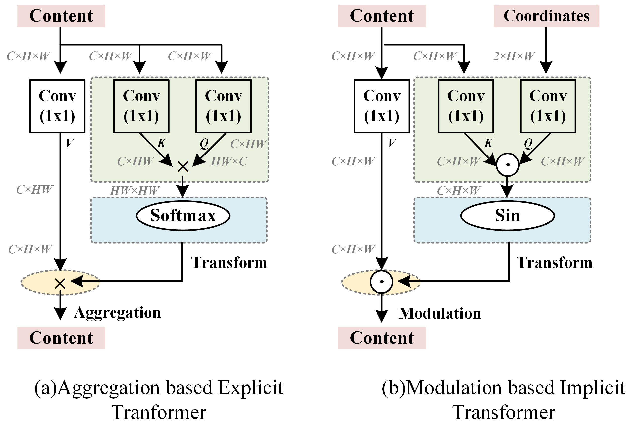
Figure 2: Illustration of aggregation based explicit transformer and modulation based implicit transformer.

3 Implicit and Enhanced Transformer Network for SCISR

In this section, we first give the definition of Transformer, and then describe the design of our implicit transformer based upsampler, followed by illustrating the proposed enhanced transformer based feature extraction backbone.

3.1 Transformer

The key module in transformer network is the (multi-head) self attention [29], which can be expressed as

$$z=\text{Softmax}(QK^{T}/\sqrt{D}+B)V,$$ (1)

where $Q$, $K$, and $V$ denote the query, key, and value respectively. $B$ is the position encoding and $D$ is the dimension of $Q$ and $K$. $z$ is the token (i.e., $V$) aggregation result with the weights calculated based on the normalized “distance” between $Q$ and $K$. For multi-head self-attention, this process is performed for $h$ (the head number) times parallelly and the results are concatenated along the $D$ dimension. In this work, we reformulate the transformer into a more general form, i.e.,

$$z=\Phi(Q,K)\otimes V,$$ (2)

where $\Phi(Q,K)$ denotes the weights calculated by $Q$ and $K$, and $\otimes$ represents matrix multiplication or point-wise multiplication. When $\otimes$ represents matrix multiplication and $V$ is a set of multiple token features (namely $V=[V_{1},V_{2},...,V_{m}]$), Eq. 2 is an aggregation transformer, where the result $z$ is the aggregation of different tokens $\{V_{i}\}$. When $\otimes$ represents point-wise multiplication ($\odot$) and $V$ is a single token feature (namely $V=V_{i}$), Eq. 2 is a modulation transformer and the result $z$ is the modulation of the current input $V_{i}$.

In the literature, the predominant transformer is the aggregation transformer. Here, we denote it as explicit transformer, where $Q$, $K$, and $V$ are inferred from the same kind of inputs. For example, in SwinIR [8], $Q$ is the linear transform of the current token (feature) while $K$ and $V$ are the linear transform of its neighboring tokens (features). In contrast, for implicit transformer, we mean $Q$ is derived from coordinates while $V$ is derived from pixel values, similar to the implicit function defined in Nerf [18]. Correspondingly, in this work, we propose the modulation transformer to module the implicit transformer. Figure 2 presents the summarization of the two kinds of transformers.

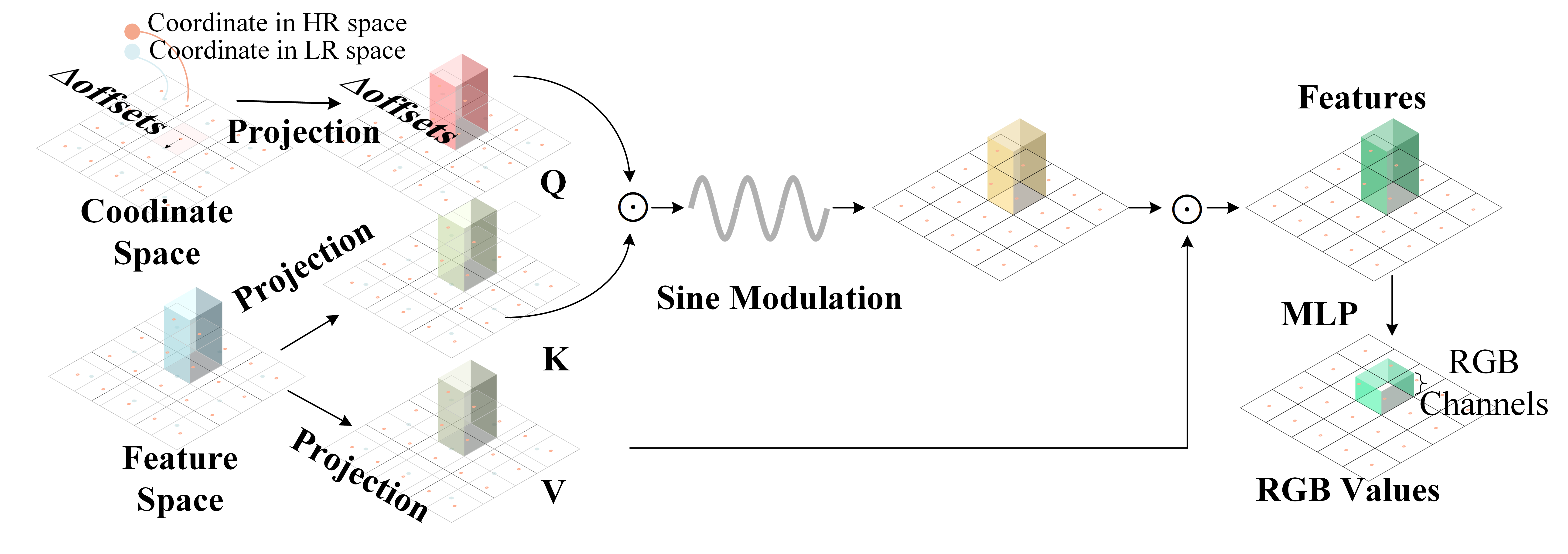
Figure 3: The proposed implicit transformer based upsampler, which can generate pixel values in continuous space. The orange coordinates are in HR space and the blue coordinates are in LR space.

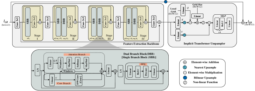
Figure 4: Detailed network architecture of the proposed ITSRN++. Our model includes two parts: enhanced transformer based feature extraction backbone and implicit transformer based upsampler. The feature extraction backbone contains four stages, with dual branch block and single branch block. The DBB is constructed by attention branch and conv branch. Removing the attention branch (circled by dotted line) and changing the conv block to dwconv block resulting in SBB.

3.2 Implicit Transformer Based Upsampler

Before introducing our upsampling scheme, we first revisit the image upsampling process. If we view image upsampling in a continuous space, it can be seen as sampling values at discrete points within a finite area. For image interpolation, suppose that we have an LR image $I_{LR}$ that needs to be upsampled. The pixel value of query point $q(i,j)$ in the HR image $I_{HR}$ is obtained by fusing pixel values of its neighboring key points $k(\Omega(i),\Omega(j))$ in $I_{LR}$ with weighting coefficients, where $\Omega(i)$ denotes the neighboring points of $i$ in $I_{LR}$. Denoting the query points in upsampled image as $Q$, the key points in the input LR image as $K$, and the value on the corresponding key points as $V$, the image upsampler can be reformulated as Eq. 2, i.e., an aggregation transformer [29]. Instead of utilizing pixel features to generate $Q$ and $V$, the interpolation transformer deals with pixels’ coordinates and their values. Inspired by the implicit function in NeRF [18], which utilizes the pixel coordinates to generate RGB values, we rename the interpolation process as Implicit Transformer, and propose a novel Implicit Transformer Network for SCI SR.

Specifically, we redesign the upsampling process as

$$\textit{Offsets}=P_{HR}-P^{*}_{LR},\quad Q=\text{Linear}(\textit{Offsets}),$$

$$K=\text{Linear}(\mathcal{F}_{LR}),\quad V=\text{Linear}(\mathcal{F}_{LR}),$$ (3)

where $\textit{Offsets}\in\mathbb{R}^{H\times W\times 2}$ denotes the relative offsets between the query points in the HR space ($P_{HR}$) and their corresponding nearest neighboring points ($P^{*}_{LR}$) in the LR space, as shown in Fig. 3 (the orange pixel in the HR space has a nearest neighbor in the LR space denoted by blue pixel). To ease the training process, we normalize the coordinates into the range of [-1, 1]. Different from [13, 14, 15], which directly predict (using the function $\Phi(\cdot)$) the continuous representation with the relative coordinate $p_{q}-p^{*}_{k}$, we treat it as query to perform local continuous representation. We project the Offsets to $Q\in\mathbb{R}^{H\times W\times C}$ with a linear transform, and project the deep features (denoted as $\mathcal{F}_{LR}$) extracted from the LR input to $K,V\in\mathbb{R}^{H\times W\times C}$ with another two linear transforms. For the query point $p$ (in the continuous HR space), the query feature is $Q_{p}$, and its corresponding key and value in the LR space is $K_{p^{*}}$ and $V_{p^{*}}$, where ${{p^{*}}}$ represents the nearest neighboring point of $p$. We observe that utilizing the aggregation of different ${V_{i}}$ to predict pixel value may lead to smoothness due to the low-pass characteristics of the weighted aggregation process. Therefore, we propose the modulation transformer as follows:

$$I_{p}=\Phi(\sigma(K_{{p^{*}}}\odot Q_{p}+\text{Linear}(S))\odot V_{p^{*}}),$$ (4)

where $\sigma$ is the nonlinear mapping function, and $\Phi$ represents an MLP with four layers. The element-wise multiplication between $K_{p^{*}}$ and $Q_{p}$ generates the attention weight $\in\mathbb{R}^{1\times 1\times C}$. Similar to [30], we further introduce a scale bias $S\in\mathbb{R}^{1\times 1\times 2}$, which refers the scaling factor along $H$ and $W$ dimension, respectively. We project $S$ with a linear layer to make it have the same dimension ($1\times 1\times C$) as that of the weights. To reweight the attention matrix, many non-linear mapping functions can be adopted, such as Softmax, Sigmoid, and Tanh. However, these are all monotone increasing functions, which may limit the non-linear mapping space. Some works [51, 52] demonstrate that the periodic activation functions can facilitate networks to learn high-frequency information. Therefore, we propose to utilize a periodic function to reweight the attention values. In this work, we utilize $sin(\cdot)$ as the nonlinear mapping function to reweight the weights. Hereafter, we modulate the value $V$ with the recalibrated weights via point-wise multiplication. In other words, $V_{p}$ is a modulated version of $V_{p^{*}}$. The features in discrete space can be modulated to features in continuous space by the learned non-linear weights. Finally, we use an MLP to map the feature $V_{p}$ to pixel value $I_{p}$. The whole process is illustrated in Fig. 3.

Utilizing Eq. 4 to generate the pixel value can get rid of the influence of its neighboring pixels. This is beneficial for high-frequency detail generation but it may lead to discontinuity. Therefore, we further propose to utilize a local filter to refine the results. This process is denoted as:

$$\hat{I}_{q}=\sum_{p\in\Omega_{(}q)}\omega(p,q)I_{q},$$ (5)

where $\hat{I}_{q}$ is the refined pixel value. $\Omega(q)$ is a local window centered at $q$, and $w$ represents the neighbors’ (denotes by $p$) contribution to the target pixel. In this work, we directly utilize the bilinear filter as the weighting parameter $w$.

We would like to point out that our upsampler in this work is totally different from LIIF and ITSRN. 1) Relationship with LIIF. In implicit function based SR method LIIF [13], $K$ is the nearest neighbor coordinate in $I^{L}$ for the corresponding $Q$ in $I^{H}$, and $V$ is the corresponding deep features of $K$. Different from ours, the super-resolved pixel value $I_{q}$ is obtained by concatenating $V$ and the relative offsets between $Q$ and $K$ first and then going through the nonlinear mapping $\Phi$ (realized by an MLP). It has achieved promising results due to the strong fitting ability of the MLP. However, we observe that directly concatenating the extracted pixel features and the relative coordinates is not optimal and this will lead to a large resolution space. Therefore, we utilize $\Phi(Q,K)V$ other than $\Phi(Q,K,V)$ for upsampling. In this way, we constrain the features in continuous space to be a variant of its neighboring feature in the discrete space and the pixel value is inferred from the modulated features. 2) Relationship with ITSRN. In our previous work, we model the upsampler as

$$I=\Phi(Q,K)V=H(Q-K)V,$$ (6)

where $H(Q-K)$ maps the relative offsets between the HR coordinates and the corresponding LR coordinates to high-dimensional weights, which are then multiplied with the deep pixel features $V$ to generate the pixel value $I$. However, it consumes lots of memory and $H(Q-K)$ cannot be adaptive according to the image contents. In contrast, our upsampling weights in Eq. 4 can be adaptive according to the image contents.

3.3 Enhanced Transformer Based Feature Extraction

As shown in Eq. 3 and 4, the upsampling results heavily depend on the extracted features $\mathcal{F}_{LR}$. In this work, we propose an enhanced transformer based feature extraction backbone, which is constructed by cascaded dual-branch block (DBB) and single-branch block (SBB), as shown in Figure 4. In the following, we first give an overview of the network structure and then present the details of the proposed DBB and SBB.

Network Overview. Our feature extraction backbone is constructed based on Swin Transformer [30], and we incorporate several key modifications to model the sharp edges of screen content images. Following [8], for the input low-resolution image $I_{LR}\in\mathbb{R}^{H\times W\times C_{in}}$, where $H$, $W$, and $C_{in}$ are the height, width, and channels of the input image, respectively, we utilize one $3\times 3$ convolution layer to extract its shallow feature $\mathcal{F}_{s}\in\mathbb{R}^{H\times W\times C}$. Then $\mathcal{F}_{s}$ goes through the deep feature extraction module to generate the final features $\mathcal{F}_{LR}$ for the LR input. The deep feature extraction module contains four stages, and each stage contains $(1-\alpha)N\times$ SBB, $\alpha N\times$ DBB, and one $3\times 3$ convolution layer.

Dual Branch Block. As mentioned in Section 3.1, the classical transformer block, which is constructed by multi-head-self-attention (MHSA) and feed-forward network (FFN) tends to generate smoothed results since the fusion coefficients generated by Softmax function are all positive values. Therefore, we propose to introduce a convolution branch to enrich the feature representations of the transformer block, constructing the Dual Branch (attention branch and conv branch) Block:

$$\text{DBB}(\mathcal{F})=\text{Attention}(\mathcal{F})+\text{Conv}(\mathcal{F}),$$ (7)

where $\mathcal{F}$ is the input feature map $\in\mathbb{R}^{H\times W\times C}$. Specifically, our attention branch is similar to that in [8][30]. At each stage, the input feature map $\mathcal{F}$ is projected to $Q,K,V$ with linear transform layers, where $H\times W$ is the token number (i.e., a point is a token) and $C$ is the channel number. These tokens are further partitioned into non-overlapped $M\times M$ windows, and the window number is $HW/M^{2}$. Therefore, in each window, there are $M^{2}$ tokens and the dimension of each token is $D$. Then, the self-attention is calculated within the local window, namely

$$\text{Attention}(Q,K,V)=\text{Softmax}(QK^{T}/\sqrt{D}+B)V,$$ (8)

where $B\in\mathbb{R}^{M^{2}\times M^{2}}$ is the learnable relative position bias. To reduce the computing complexity, following [30], we perform the attention process parallelly for $h$ times and they are concatenated along the $D$ dimension, constructing MHSA. We denote the features after the MHSA as $\mathcal{F}_{\text{MHSA}}$. Since the windows are not overlapped, there are no connections among different windows. Therefore, following the shifting window strategy proposed in [30] to merge information across local windows, we stack regular and shifted partitions sequentially along the layers. Note that, the shifted window partitioning denotes shifting the tokens by half size of the windows.

For the convolution branch, different from  [53, 54, 55], which perform convolution with the input features, we instead extract the convolution features from the value $V$, which is not partitioned into windows. In this way, the convolution layer can explore the correlations among neighboring windows, which further enhances the correlations of tokens along the window borders. In DBB, We use DWConvBlock (DWConv(k=5)-Relu-Conv(k=1)-CA) as Conv(). After going through the depth-wise convolution, point-wise convolution, and channel attention layers, we obtain the conv features $\mathcal{F}_{\text{conv}}$. Then, $\mathcal{F}_{\text{conv}}$ and $\mathcal{F}_{\text{MHSA}}$ are added together, going through another linear layer. Hereafter, a multi-layer perceptron (MLP) that has two fully connected layers with ReLU non-linearity between them is used as FFN for further feature aggregation. Besides, a pre LayerNorm (LN) layer is inserted before FFN and MHSA+Conv modules, and the residual skip connection is added for both blocks, as shown in Figure 4.

Single Branch Block. Note that, DBB consumes lots of memory and computing resources. To reduce the computing complexity, we also construct the single branch block (SBB), where the attention branch (circled by a dotted line in Figure 4) is removed. In this case, We replace the DWConvBlock with ConvBlock(Conv(k=3)-ReLU-Conv(k=3)-CA). For earlier stages, we utilize more SBBs to extract visual features while in later stages we utilize more DBBs to enhance the feature aggregation process. The ratios ($\alpha_{2}$,$\alpha_{3}$,$\alpha_{4}$) between the number of DBB and SBB are explained in the experiments.

Figure 5 presents the frequency statistics of the features learned in convolution branch and attention branch. Take the features in the second DBB for example, we perform Fourier transform on the features $\mathcal{F}_{\text{conv}}$ and $\mathcal{F}_{\text{MHSA}}$, and the features along different channels are averaged. It can be observed that the features learned by the conv-branch contain more high-frequency information compared with those learned by the attention-branch. In this way, the conv-branch feature is a good complementary of the attention-branch feature.

Convolution-Branch	Attention-Branch

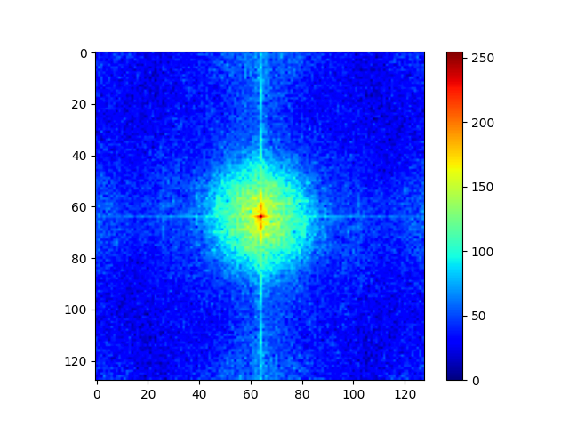
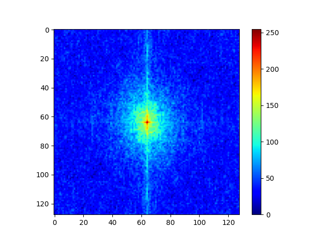
Figure 5: Centralized Fourier spectrum of conv-branch feature and attention-branch feature in the second DBB. Note that, the brighter the color, the greater the amplitude of the Fourier spectrum.

3.4 Multi-scale Training

To enable multi-scale training, we construct the mini-batch with upsamping scales uniformly sampled from $\mathcal{U}(1,4)$. Let $r$ denote the scaling factor, and $h,w$ are the height and width of the LR patch. We first crop the HR patch with a size of $rh\times rw$ from the HR image to serve as ground truth (GT). Then we generate its LR counterpart by downsampling the GT with the scale factor $r$ via bicubic interpolation. Finally, we randomly sample $hw$ pixels from each GT patch to make the GTs in a batch have the same size. Meanwhile, for a batch of LR inputs, they share the same size but have different magnification ratios. Compared with training with a single magnification factor for each batch, multi-scale training is more stable and leads to better results.

During training, we utilize the most popular $\ell_{1}$ loss function, namely

$$\mathcal{L}=\left\|I_{SR}-I_{HR}\right\|_{1},$$ (9)

where $I_{SR}$ is the SR result, and $I_{HR}$ is the GT image.

4 SCI2K dataset

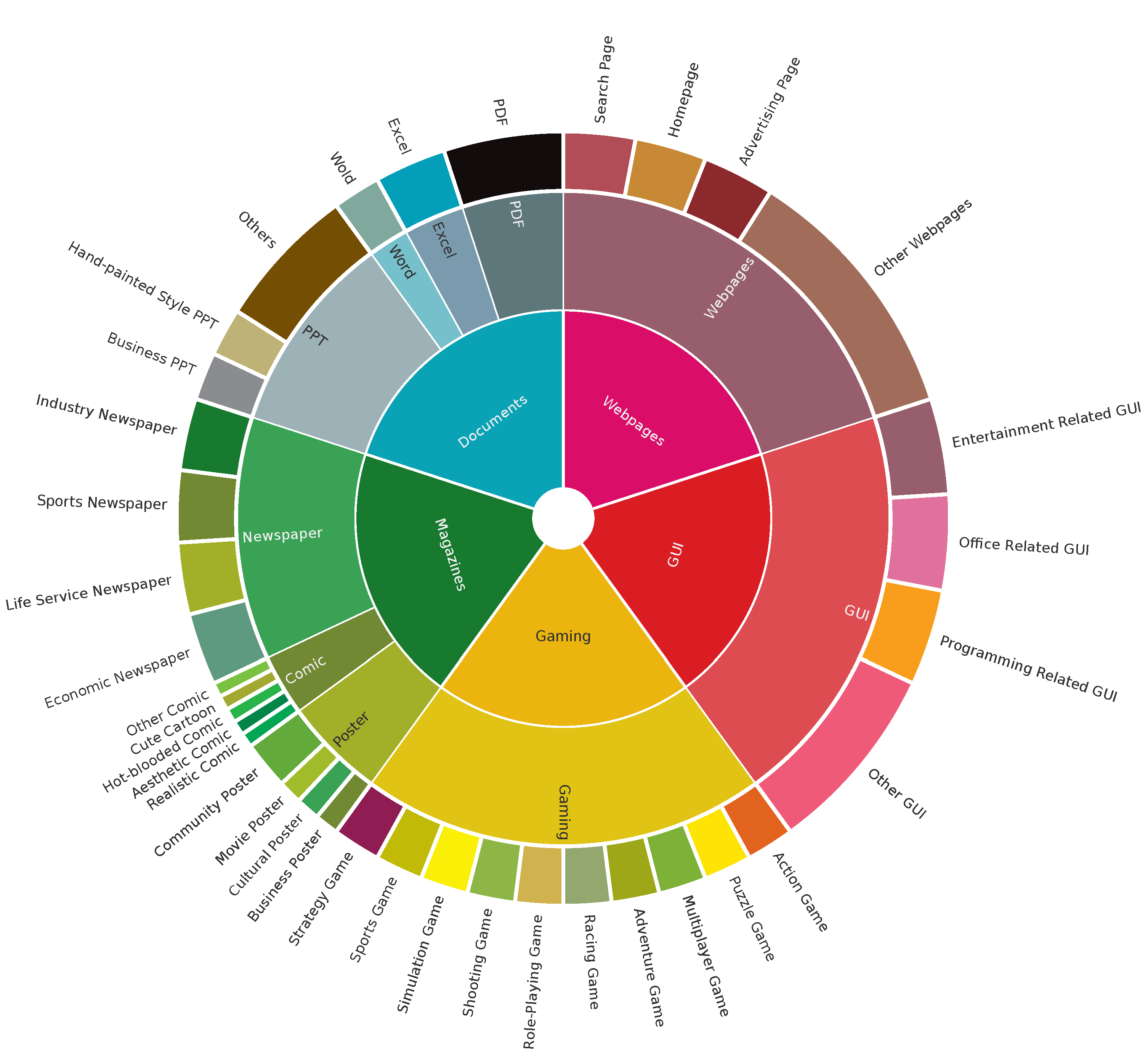
Figure 6: The radial dendrogram of our SCI2K dataset, which contains five main categories of screen contents.

Compared with the datasets for natural image SR, such as DIV2K [56], Urban100 [57], and BSDS100 [58], datasets for SCIs are limited and most of them are for quality assessment. For example, the SIQAD dataset [46], designed for image quality assessment, contains 20 ground truth images (with resolution around $600\times 800$) and 980 distorted images. The SCID [48] dataset consists of 40 screen content images (with a resolution of $1280\times 720$) and 1800 distorted images. The CCT dataset [59] consists of three kinds of image contents, i.e., natural scene image, computer graphic image, and screen content image, with 24 reference images for each type. However, the image resolutions in the three datasets are mostly less than 1K and the image amount for high-quality reference images is far from enough for training SR networks. Our previous work ITSRN [14] constructs the first SCI SR dataset, named as SCI1K, which contains 1000 screenshots with a resolution of $1280\times 720$ and $2560\times 1440$ (less than 100 images).

In recent years, there is a trend to train larger models with larger datasets, and the image resolution is also increased. For example, for natural image SR, the DIV2K dataset [56], which contains 1000 images with a resolution of 2K is widely used. Some transformer-based works [8] further utilize the combination of DIV2K and Flickr2K datasets to boost the SR results. In contrast, there is still no large-scale SCI dataset. On the hand, to cope with the development of large screens, an SCI SR dataset with a larger resolution is demanded. Therefore, in this work, we construct an SCI2K dataset, which contains 2000 images with 2K resolution, by manually capturing the screen content with the snipping tool in Windows 10. Figure 6 lists the detailed categories of our dataset, which covers various contents, including documents, magazines, webpages, game scenes, etc, which are common cases in our daily life.

The 2000 images are randomly split into train and test sets, which contain 1800 and 200 images, respectively. To be consistent with previous works, the LR images are synthesized by bicubic downsampling. To further simulate the compression degradations caused by transmission and storage, we further construct the SCI2K-compression dataset by applying JPEG compression on the LR images. The quality factors are randomly selected from 75, 85, and 95.

5 Experiments

5.1 Implementation and Training Details

Datasets. For SCI SR, we use our proposed SCI2K dataset for training. For evaluation, besides the testing set in SCI2K, we further utilize three benchmark screen datasets [59, 48, 46]. Since these datasets are not designed for the SR task, we downsample their GTs with bicubic interpolation (realized by the imresize function in PIL package) to construct LR-HR pairs.

Network Configurations. For the attention branch, the channel number for the shallow convolution layer and the last convolution layer is 64. The block numbers $N$ in the four stages are 2, 8, 8, and 16 respectively. And the channel number of four stages are 64, 64, 128 and 192, respectively. The ratios between the numbers of DBB and SBB in Stage 2-4 are $\alpha_{2}=0.25$,$\alpha_{3}=0.25$, and $\alpha_{4}=0.75$. The head number in MHSA is 8. The window size $M$ is 16.

Training Details. During the training process, the batch size is set to 16 and the LR patch size is $48\times 48$. Each epoch contains about $2,000$ iterations and the max epoch is set to 1000. Adam algorithm is used for optimization. The learning rate is initialized as 2e-4 and decayed by a factor 0.5 at the $400^{\text{th}},800^{\text{th}},900^{\text{th}},950^{\text{th}}$ epoch. The training data is augmented with rotation and flip with a probability of $0.5$.

5.2 Ablation Study

In this section, we perform ablation study to demonstrate the effectiveness of the proposed implicit transformer based upsampler and enhanced transformer based feature extraction backbone. The performances of different variants are evaluated on the testing set of the proposed SCI2K dataset and SCID dataset.

5.2.1 Ablation on Implicit Transformer

TABLE I: Ablation study on the proposed modulation-based implicit transformer by replacing it with two variants. The results are evaluated on SCI2K and SCID datasets for $\times 4$ SR.

Variants	SCI2K	SCID
	PSNR$\uparrow$ / SSIM$\uparrow$	PSNR$\uparrow$ / SSIM$\uparrow$
only V (Bilinear)	28.03 / 0.9275	24.35 / 0.8498
concatenation (LIIF’s)	31.25 / 0.9571	27.37 / 0.9073
modulation (Ours)	31.66 / 0.9597	27.84 / 0.9149

TABLE II: Ablation study on the reweighting function in implicit transformer. The results are evaluated on SCI2K and SCID datasets for $\times 4$ SR.

	SCI2K	SCID
	PSNR$\uparrow$ / SSIM$\uparrow$	PSNR$\uparrow$ / SSIM$\uparrow$
sin	31.66 / 0.9597	27.84 / 0.9149
sin $\rightarrow$ tanh	31.42 / 0.9587	27.67 / 0.9135
sin $\rightarrow$ sigmoid	31.36 / 0.9585	27.58 / 0.9120
sin $\rightarrow$ softmax	31.29 / 0.9578	27.52 / 0.9113

HR Image		Conv only	Attention only	Sequential	Parallel(Ours)
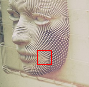
	LAM Attribution
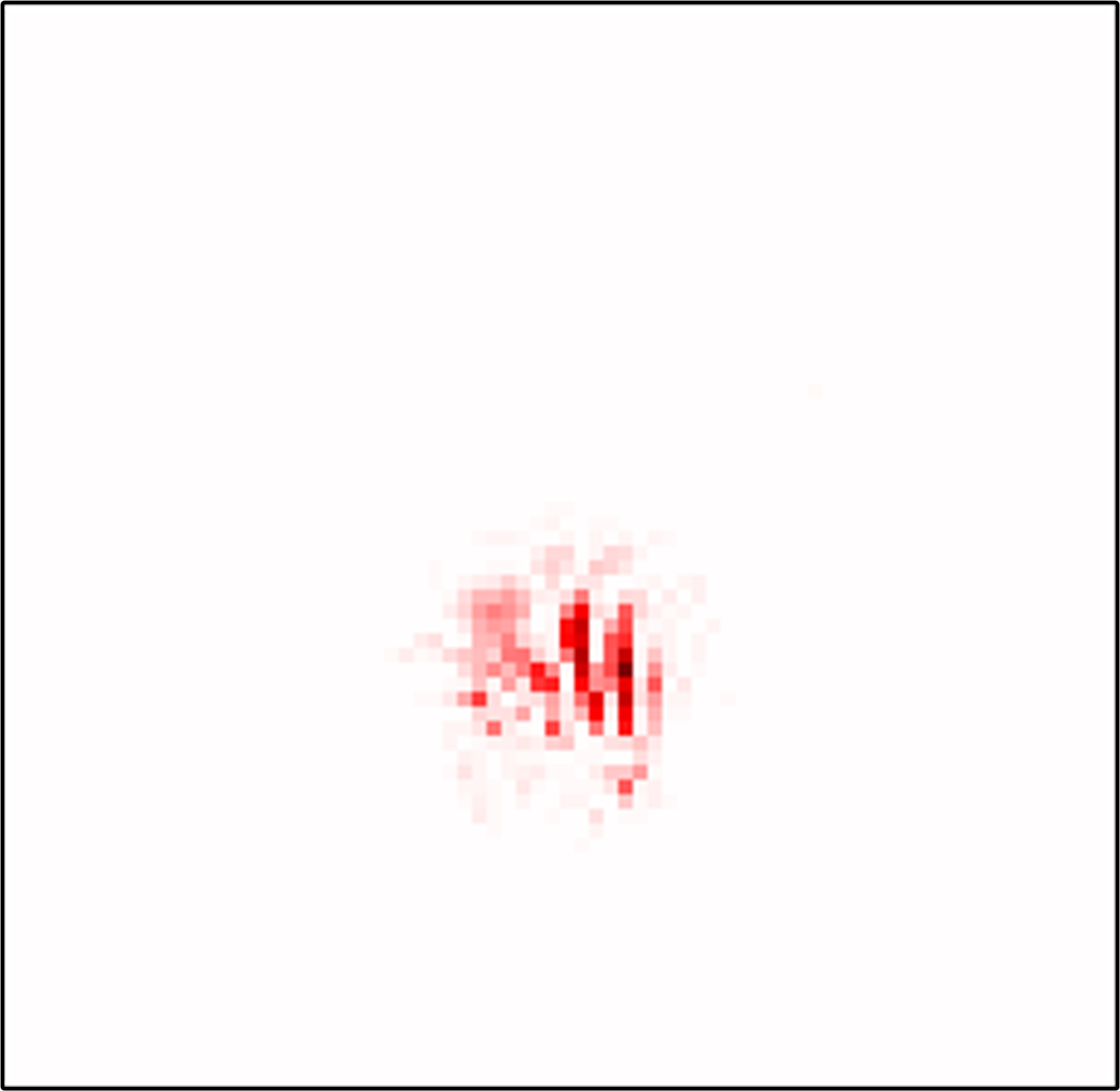
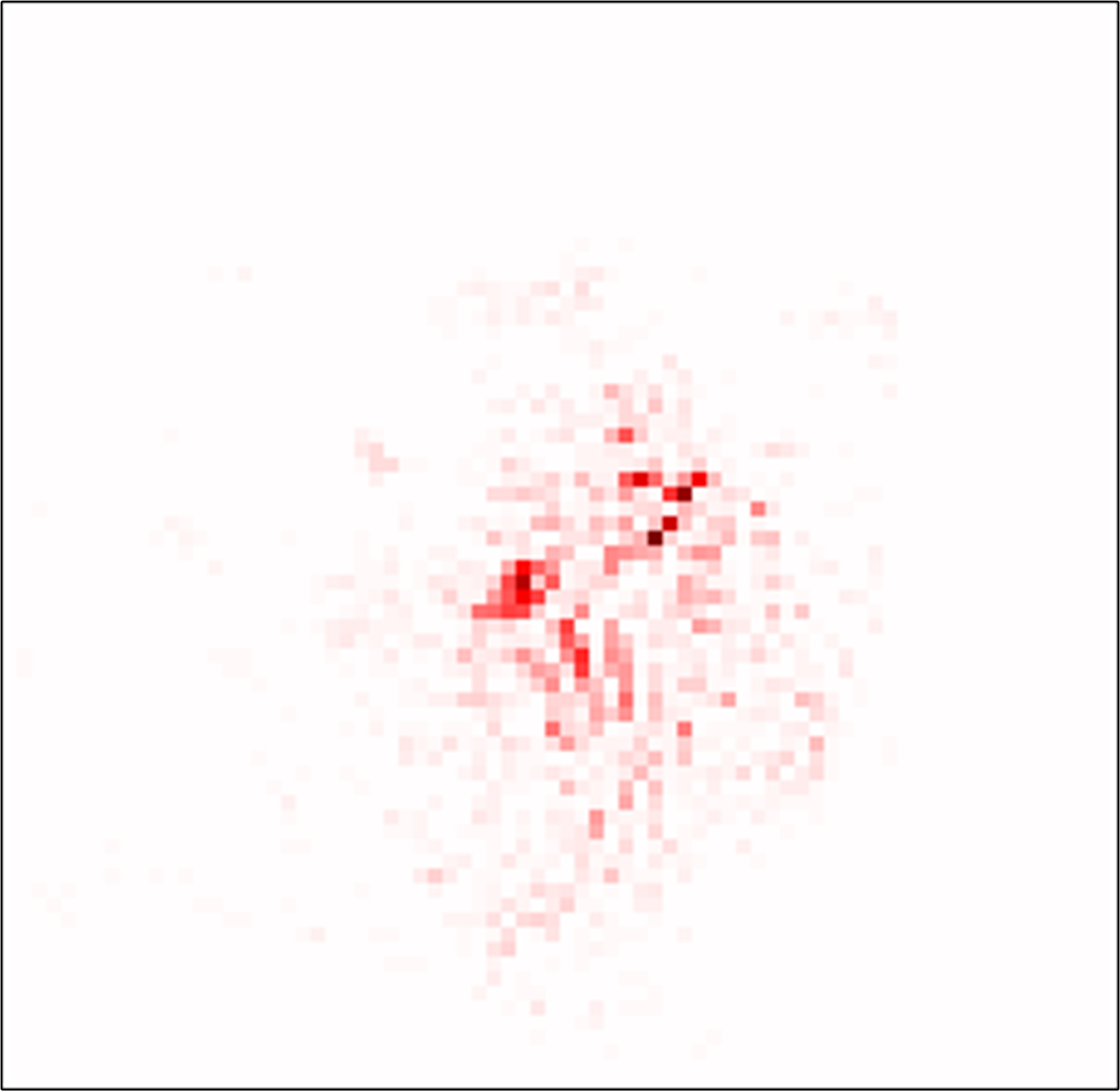
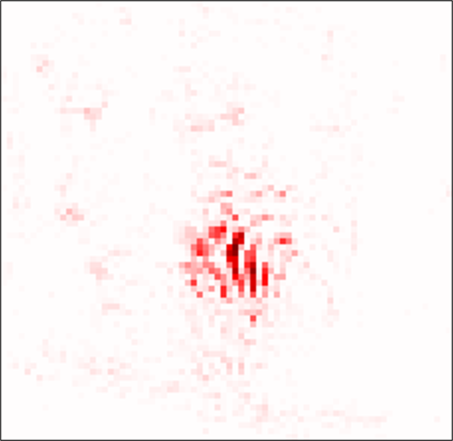
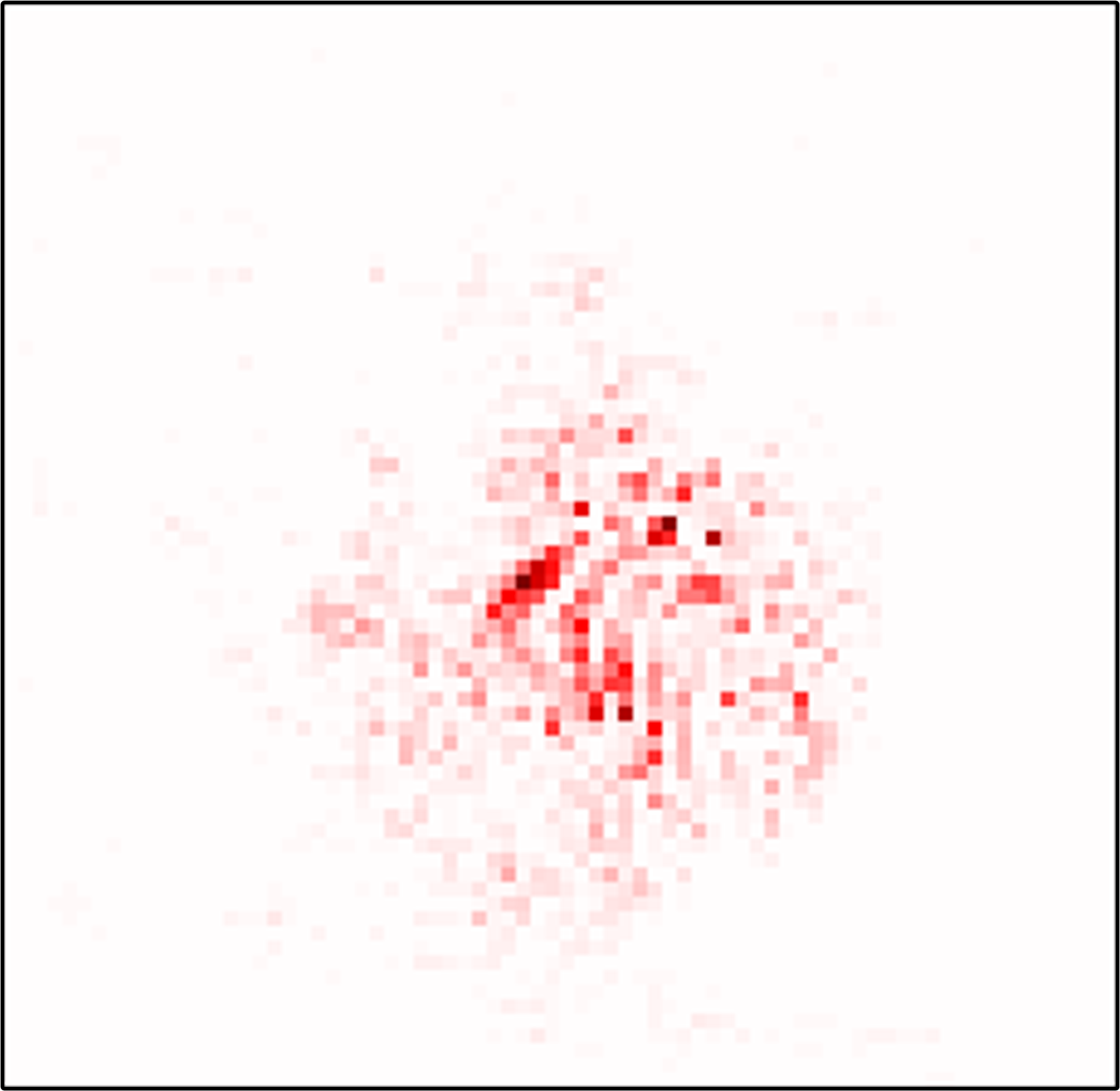
LR Image		5.42	12.09	18.48	14.07
	SR Results
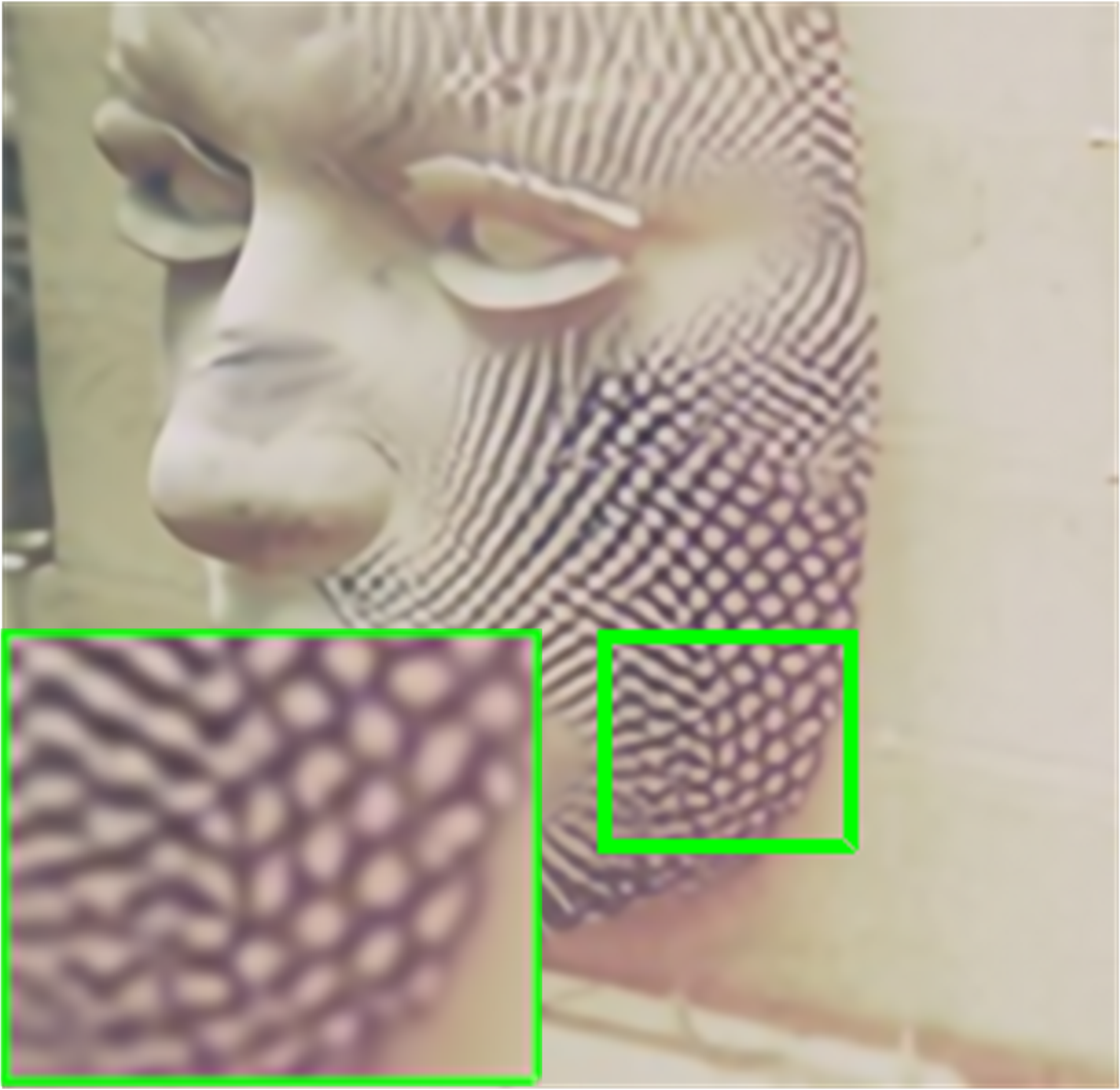
PSNR / SSIM		25.96dB / 0.7397	26.32dB / 0.7691	26.23dB / 0.7521	27.12dB / 0.7920

Figure 7: Visual comparisons for the proposed DBB and its variants. The first row is LAM [60], which highlights the pixels that contribute to the reconstruction of the patch circled by the red box. DI [60](diffusion index) values (larger values indicate more pixels are involved) for each LAM are also given. The second row is the corresponding SR results. The PSRN and SSIM results are

We first perform ablation on the proposed implicit transformer based upsampler (Eq. 4) by replacing it with two variants. The first variant is the upsampler in LIIF, namely

$$I_{p}=\Phi(\text{concat}(Q_{p},V_{p^{*}})),$$ (10)

where $\Phi(\cdot)$ is the MLP, the same as that in Eq. 4. Note that following [13], we utilize feature unfolding to enrich the information in $V$. For brevity, we still utilize $V$ to represent the enriched features.

The second variant is upsampling with only the pixel features, without utilizing the coordinates information, namely

$$I_{p}=\Phi(\text{bilinear}(V_{p^{*}})),$$ (11)

where bilinear means the values $V\in\mathbb{R}^{H\times W\times D}$ are mapped to desired resolution by bilinear interpolation. After going through the pointwise MLP $\Psi$, the values $V$ are mapped to pixel values in HR space. As shown in Table I, the proposed upsampler greatly outperforms the two variants. This demonstrates that the proposed implicit transformer based feature modulation strategy is more effective than the direct mapping strategy.

In addition, we also conduct ablation on the proposed periodic modulated function sin. We replace it by tanh, sigmoid, and softmax functions, respectively. As shown in Table II, utilizing sigmoid or softmax to perform nonlinear mapping, the performance drops more than (or around) 0.3 dB in both two test sets. The main reason is that sigmoid and softmax lead to positive values, which limit the ranges of modulated features. Correspondingly, tanh, whose output range is $[-1,1]$, generates better result than sigmoid and softmax. However, it is still lower than sin function, which demonstrates that the periodic function contributes to high-frequency learning and performance improvement.

5.2.2 Ablation on Feature Extraction Backbone

TABLE III: Ablation on the proposed Dual-Branch Block. The module ”parallel” is our proposed DBB, where conv-branch and attention-branch are in parallel. The variant ”sequential” means the two branches are stacked sequentially. ”conv only” means we only use the conv-branch in our DBB, and ”attention only” means we only adopt the attention-branch in DBB. All the results are evaluated on the SCID dataset for $\times 4$ SR.

Structure	Parameters	FLOPs	PSNR$\uparrow$	SSIM$\uparrow$
Sequential	13.98 M	320.87 G	26.92	0.9033
Attention only	13.18 M	316.32 G	27.38	0.9099
DWConv only	9.02 M	277.23 G	26.24	0.8942
Parallel DWConv on input	13.98 M	320.87 G	27.63	0.9133
Parallel DWConv on $V$ (Ours)	13.98 M	320.87 G	27.84	0.9149

Since our dual-branch block contains parallel attention and convolution branches, we replace it by transformer-block (attention branch + FFN), conv-block (conv-branch + FFN) and the sequential block, which is constructed by attention-branch+ conv-branch + FFN. For the three variants, the block number settings ($N$) and the ratio $\alpha$ are the same as that of the original setting for DBB. Table III presents the comparison results. It can be observed that the proposed parallel solution (i.e., DBB) outperforms the three variants. Compared with the sequential block, the proposed DBB achieves 0.92 dB gain. Compared with the conv block, which has larger parameters than the proposed DBB, we achieve nearly 1 dB gain.

TABLE IV: Quantitative comparison with state-of-the-art fixed-scale and continuous SR methods on SCI2K test set. In-training-scale means the upsampling ratios are included in the training pairs and out-of-training-scale means the upsampling ratios are not ”seen” during training. The fixed-scale SR methods train different models for different upsampling ratios and the continuous SR methods train one model for all the upsampling ratios. All the models are trained on the training set of SCI2K. Values in red and blue indicate the best and the second best performance, respectively.

Methods	In-training-scale			Out-of-training-scale
	$\times 2$	$\times 3$	$\times 4$	$\times 6$	$\times 12$	$\times 18$	$\times 24$	$\times 30$
Bicubic	28.32 / 0.9380	26.02 / 0.8912	24.81 / 0.8556	23.50 / 0.8116	21.67 / 0.7624	20.82 / 0.7514	20.22 / 0.7475	19.75 / 0.7450
EDSR [2]	38.68 / 0.9874	33.26 / 0.9713	29.84 / 0.9493	-	-	-	-	-
RDN [3]	38.68 / 0.9875	33.51 / 0.9716	30.25 / 0.9508	-	-	-	-	-
RCAN [4]	40.18 / 0.9886	34.19 / 0.9734	30.75 / 0.9545	-	-	-	-	-
SwinIR[8]	40.67 / 0.9890	34.79 / 0.9752	31.19 / 0.9576	-	-	-	-	-
MetaSR [12, 13]	38.82 / 0.9875	33.24 / 0.9705	29.72 / 0.9467	26.36 / 0.8950	23.40 / 0.8187	22.28 / 0.7868	21.61 / 0.7708	21.08 / 0.7610
LIIF [13]	38.85 / 0.9879	33.36 / 0.9719	29.98 / 0.9498	26.42 / 0.8986	23.44 / 0.8239	22.29 / 0.7913	21.61 / 0.7754	21.10 / 0.7654
ITSRN[14]	39.56 / 0.9883	34.11 / 0.9731	30.44 / 0.9520	26.61 / 0.9011	23.53 / 0.8243	22.36 / 0.7914	21.67 / 0.7746	21.15 / 0.7646
LTE[15]	38.89 / 0.9879	33.28 / 0.9718	29.91 / 0.9497	26.40 / 0.8998	23.48 / 0.8254	22.34 / 0.7929	21.65 / 0.7760	21.16 / 0.7663
ITSRN++	41.26 / 0.9895	35.53 / 0.9768	31.66 / 0.9597	27.17 / 0.9118	23.86 / 0.8335	22.58 / 0.7980	21.86 / 0.7797	21.33 / 0.7684

TABLE V: Quantitative comparison with state-of-the-art fixed-scale and continuous SR methods on three screen content quality assessment datasets. . All the models are trained on the training set of SCI2K. Values in red and blue indicate the best and the second best performance, respectively.

.

Dataset	Method	In-training-scale			Out-of-training-scale
		$\times$2	$\times$3	$\times$4	$\times$6	$\times$8	$\times$10
CCT[61]	EDSR [2]	31.62 / 0.9630	27.14 / 0.9171	24.67 / 0.8619	–	–	–
	RDN [3]	31.68 / 0.9648	27.26 / 0.9158	24.73 / 0.8626	–	–	–
	RCAN [4]	32.79 / 0.9703	27.74 / 0.9234	25.22 / 0.8770	–	–	–
	SwinIR [8]	33.20 / 0.9710	28.28 / 0.9332	25.50 / 0.8862	–	–	–
	MetaSR [12]	31.91 / 0.9665	27.38 / 0.9195	24.57 / 0.8597	22.24 / 0.7641	21.24 / 0.6990	20.71 / 0.6669
	LIIF [13]	32.26 / 0.9684	27.63 / 0.9240	24.75 / 0.8634	22.31 / 0.7699	21.27 / 0.7050	20.72 / 0.6723
	ITSRN[14]	32.56 / 0.9697	28.00 / 0.9267	25.07 / 0.8705	22.38 / 0.7719	21.35 / 0.7062	20.79 / 0.6727
	LTE [15]	32.51 / 0.9709	27.73 / 0.9282	24.87 / 0.8731	22.38 / 0.7781	21.37 / 0.7139	20.84 / 0.6781
	ITSRN++	34.23 / 0.9781	29.30 / 0.9452	26.29 / 0.9017	23.06 / 0.8067	21.65 / 0.7284	20.87 / 0.6795
SCID [48]	EDSR [2]	33.92 / 0.9700	29.00 / 0.9323	25.85 / 0.8873	–	–	–
	RDN [3]	34.00 / 0.9713	29.13 / 0.9317	26.11 / 0.8906	–	–	–
	RCAN [4]	34.90 / 0.9743	29.65 / 0.9358	26.59 / 0.8989	–	–	–
	SwinIR [8]	35.54 / 0.9751	30.29 / 0.9419	26.89 / 0.9037	–	–	–
	MetaSR [12]	34.11 / 0.9719	29.24 / 0.9331	25.99 / 0.8891	22.65 / 0.7941	21.25 / 0.7238	20.58 / 0.6867
	LIIF [13]	34.22 / 0.9728	29.38 / 0.9350	26.22 / 0.8932	22.69 / 0.8007	21.29 / 0.7315	20.59 / 0.6925
	ITSRN [14]	34.67 / 0.9739	29.98 / 0.9378	26.68 / 0.8974	22.86 / 0.8029	21.36 / 0.7335	20.65 / 0.6933
	LTE [15]	34.54 / 0.9746	29.54 / 0.9383	26.24 / 0.8972	22.74 / 0.8053	21.38 / 0.7389	20.67 / 0.6980
	ITSRN++	36.07 / 0.9788	31.14 / 0.9487	27.84 / 0.9149	23.63 / 0.8324	21.65 / 0.7478	20.71 / 0.6948
SIQAD [46]	EDSR [2]	33.58 / 0.9806	27.95 / 0.9462	23.95 / 0.8891	–	–	–
	RDN [3]	33.68 / 0.9807	28.07 / 0.9455	24.37 / 0.8930	–	–	–
	RCAN [4]	34.79 / 0.9828	29.02 / 0.9515	25.01 / 0.9040	–	–	–
	SwinIR [8]	35.35 / 0.9829	29.57 / 0.9553	25.39 / 0.9102	–	–	–
	MetaSR [12]	34.13 / 0.9818	28.42 / 0.9479	23.82 / 0.8831	20.24 / 0.7418	19.34 / 0.6729	18.77 / 0.6263
	LIIF [13]	34.23 / 0.9821	28.55 / 0.9494	24.09 / 0.8899	20.26 / 0.7479	19.34 / 0.6772	18.73 / 0.6309
	ITSRN [14]	34.92 / 0.9832	29.56 / 0.9541	24.70 / 0.8981	20.38 / 0.7536	19.41 / 0.6811	18.82 / 0.6340
	LTE [15]	34.52 / 0.9830	28.54 / 0.9505	24.01 / 0.8919	20.29 / 0.7538	19.39 / 0.6816	18.82 / 0.6354
	ITSRN++	36.06 / 0.9852	31.11 / 0.9618	26.47 / 0.9220	20.98 / 0.7869	19.62 / 0.6947	18.88 / 0.6346

TABLE VI: Quantitative evaluation on SCI2K-compression dataset for $\times 4$ SR. All the models are trained on the training set of SCI2K-compression and evaluated on the compressed test set of SCI2K, with the compression quality factor setting to 75, 85, and 95 respectively. Values in red and blue indicate the best and the second best performance, respectively.

Method	Compression Factor
	$q=75$	$q=85$	$q=95$
RCAN [4]	27.11 / 0.9093	27.83 / 0.9210	28.61 / 0.9335
SwinIR [8]	27.34 / 0.9134	28.10 / 0.9250	28.93 / 0.9375
MetaSR [12]	26.93 / 0.9029	27.41 / 0.9142	28.02 / 0.9262
LIIF [13]	26.90 / 0.9035	27.53 / 0.9154	28.18 / 0.9271
ITSRN[14]	27.11 / 0.9076	27.82 / 0.9197	28.56 / 0.9318
LTE [15]	26.94 / 0.9057	27.59 / 0.9175	28.32 / 0.9302
ITSRN++	27.60 / 0.9168	28.40 / 0.9289	29.34 / 0.9419

Figure 7 presents the visual comparison results and the corresponding local attribution maps (LAM) [60] of the three variants and our method. The first row presents the LAM results, where the red points denote pixels that contribute to the reconstruction. It can be observed that when only using convolution, the region of LAM is the smallest. It indicates that the convolution operation is good at utilizing local correlations due to its inductive bias. The attention-only variant has a larger LAM since self-attention can explore long-range correlations, and it achieves better results than the conv-only variant. The sequential connection variant has the largest LAM region. However, many uncorrelated pixels are also involved and this leads to worse results compared with the attention-only variant. In contrast, our proposed parallel solution leads to a larger LAM region, and the pixels inside LAM are all correlated with the target patch. Therefore, the proposed parallel strategy achieves the best reconstruction result.

Ground-truth HR SCI2K: img1999 HR Bicubic RDN [3] RCAN [4] SwinIR [8] MetaSR [12] LIIF [13] LTE [15] ITSRN [14] ITSRN++(ours)

Ground-truth HR CCT: img023 HR Bicubic RDN [3] RCAN [4] SwinIR [8] MetaSR [12] LIIF [13] LTE [15] ITSRN [14] ITSRN++(Ours)

Ground-truth HR SCID: img032 HR Bicubic RDN [3] RCAN [4] SwinIR [8] MetaSR [12] LIIF [13] LTE [15] ITSRN [14] ITSRN++(Ours)

Ground-truth HR SIQAD: img017 HR Bicubic RDN [3] RCAN [4] SwinIR [8] MetaSR [12] LIIF [13] LTE [15] ITSRN [14] ITSRN++(Ours)

Figure 8: Visual comparison for $\times 4$ SR on the SCI2K, CCT, SIQAD, and SCID datasets.

TABLE VII: Quantitative evaluation of state-of-the-art SR methods on five benchmark SR datasets. All the models are trained on the DIV2K dataset.. The dashed line is used to separate fixed-scale and continuous SR methods. The results for fixed-scale SR methods are generated with models trained with $\times 2,\times 3,\times 4$ and $\times 8$ LR-HR pairs, respectively. The results for continuous SR methods are generated with one model trained with continuous random scales uniformly sampled from $\times 1$ $\times 4$ LR-HR pairs. All results are quoted from their original papers, except MetaSR and LIIF (indicated by ^†). For them, we utilize the results reported in [15], which changes their feature extraction backbone to SwinIR. Since CSNLN [23], IGNN[62] NSLN [22], and ENLCN [24] did not report their $\times 8$ results, we omit them. Values in red and blue indicate the best and the second best performance, respectively.

Method	Year	Scale	Set5	Set14	BSDS100	Urban100	Manga109
			PSNR / SSIM	PSNR / SSIM	PSNR / SSIM	PSNR / SSIM	PSNR / SSIM
Bicubic	–	$\times$2	33.66 / 0.9299	30.24 / 0.8688	29.56 / 0.8431	26.88 / 0.8403	30.80 / 0.9339
EDSR [2]	2017	$\times$2	38.11 / 0.9602	33.92 / 0.9195	32.32 / 0.9013	32.93 / 0.9351	39.10 / 0.9773
RCAN [4]	2018	$\times$2	38.27 / 0.9614	34.12 / 0.9216	32.41 / 0.9027	33.34 / 0.9384	39.44 / 0.9786
CSNLN [23]	2020	$\times$2	38.28 / 0.9616	34.12 / 0.9223	32.40 / 0.9024	33.25 / 0.9386	39.37 / 0.9785
IGNN [62]	2020	$\times$2	38.24 / 0.9613	34.07 / 0.9217	32.41 / 0.9025	33.23 / 0.9383	39.35 / 0.9786
HAN [20]	2020	$\times$2	38.27 / 0.9614	34.16 / 0.9217	32.41 / 0.9027	33.35 / 0.9385	39.46 / 0.9785
NLSN [22]	2021	$\times$2	38.34 / 0.9618	34.08 / 0.9231	32.43 / 0.9027	33.42 / 0.9394	39.59 / 0.9789
SwinIR [8]	2021	$\times$2	38.35 / 0.9620	34.14 / 0.9227	32.44 / 0.9030	33.40 / 0.9393	39.60 / 0.9792
ENLCN [24]	2022	$\times$2	38.37 / 0.9618	34.17 / 0.9229	32.49 / 0.9032	33.56 / 0.9398	39.64 / 0.9791
SwinIR-MetaSR† [8, 12]	2019	$\times$2	38.12 / 0.9614	34.09 / 0.9227	32.35 / 0.9021	33.23 / 0.9387	39.29 / 0.9784
SwinIR-LIIF† [8, 13]	2021	$\times$2	38.15 / 0.9615	34.09 / 0.9223	32.35 / 0.9020	33.31 / 0.9389	39.38 / 0.9786
SwinIR-LTE [15]	2022	$\times$2	38.21 / 0.9616	34.19 / 0.9234	32.39 / 0.9026	33.45 / 0.9405	39.44 / 0.9786
ITSRN++	–	$\times$2	38.30 / 0.9619	34.41 / 0.9236	32.45 / 0.9032	33.79 / 0.9423	39.69 / 0.9791
Bicubic	–	$\times$3	30.39 / 0.8682	27.55 / 0.7742	27.21 / 0.7385	24.46 / 0.7349	26.95 / 0.8556
EDSR [2]	2017	$\times$3	34.65 / 0.9280	30.52 / 0.8462	29.25 / 0.8093	28.80 / 0.8653	34.17 / 0.9476
RCAN [4]	2018	$\times$3	34.74 / 0.9299	30.65 / 0.8482	29.32 / 0.8111	29.09 / 0.8702	34.44 / 0.9499
CSNLN [23]	2020	$\times$3	34.74 / 0.9300	30.66 / 0.8482	29.33 / 0.8105	29.13 / 0.8712	34.45 / 0.9502
IGNN [62]	2020	$\times$3	34.72 / 0.9298	30.66 / 0.8484	29.31 / 0.8105	29.03 / 0.8696	34.39 / 0.9496
HAN [20]	2020	$\times$3	34.75 / 0.9299	30.67 / 0.8483	29.32 / 0.8110	29.10 / 0.8705	34.48 / 0.9500
NLSN [22]	2021	$\times$3	34.85 / 0.9306	30.70 / 0.8485	29.34 / 0.8117	29.25 / 0.8726	34.57 / 0.9508
SwinIR [8]	2021	$\times$3	34.89 / 0.9312	30.77 / 0.8503	29.37 / 0.8124	29.29 / 0.8744	34.74 / 0.9518
ENLCN [24]	2022	$\times$3	–	–	–	–	–
SwinIR-MetaSR† [8, 12]	2019	$\times$3	34.70 / 0.9300	30.64 / 0.8498	29.29 / 0.8115	29.10 / 0.8728	34.57 / 0.9508
SwinIR-LIIF† [8, 13]	2021	$\times$3	34.81 / 0.9306	30.72 / 0.8503	29.33 / 0.8123	29.31 / 0.8753	34.64 / 0.9514
SwinIR-LTE [15]	2022	$\times$3	34.83 / 0.9309	30.77 / 0.8513	29.37 / 0.8128	29.40 / 0.8768	34.75 / 0.9519
ITSRN++	–	$\times$3	34.90 / 0.9315	30.94 / 0.8523	29.40 / 0.8137	29.67 / 0.8802	35.02 / 0.9529
Bicubic	–	$\times$4	28.42 / 0.8104	26.00 / 0.7027	25.96 / 0.6675	23.14 / 0.6577	24.89 / 0.7866
EDSR [2]	2017	$\times$4	32.46 / 0.8968	28.80 / 0.7876	27.71 / 0.7420	26.64 / 0.8033	31.02 / 0.9148
RCAN [4]	2018	$\times$4	32.63 / 0.9002	28.87 / 0.7889	27.77 / 0.7436	26.82 / 0.8087	31.22 / 0.9173
CSNLN [23]	2020	$\times$4	32.68 / 0.9003	28.95 / 0.7888	27.80 / 0.7439	27.22 / 0.8168	31.43 / 0.9201
IGNN [62]	2020	$\times$4	32.57 / 0.8998	28.85 / 0.7891	27.77 / 0.7434	26.84 / 0.8090	31.28 / 0.9182
HAN [20]	2020	$\times$4	32.64 / 0.9002	28.90 / 0.7890	27.80 / 0.7442	26.85 / 0.8094	31.42 / 0.9177
NLSN [22]	2021	$\times$4	32.59 / 0.9000	28.87 / 0.7891	27.78 / 0.7444	26.96 / 0.8109	31.27 / 0.9184
SwinIR [8]	2021	$\times$4	32.72 / 0.9021	28.94 / 0.7914	27.83 / 0.7459	27.07 / 0.8164	31.67 / 0.9226
ENLCN [24]	2022	$\times$4	32.67 / 0.9004	28.94 / 0.7892	27.82 / 0.7452	27.12 / 0.8141	31.33 / 0.9188
SwinIR-MetaSR† [8, 12]	2019	$\times$4	32.43 / 0.8985	28.83 / 0.7898	27.74 / 0.7440	26.75 / 0.8094	31.34 / 0.9187
SwinIR-LIIF† [8, 13]	2021	$\times$4	32.69 / 0.9017	28.96 / 0.7914	27.82 / 0.7457	27.13 / 0.8164	31.69 / 0.9222
SwinIR-LTE [15]	2022	$\times$4	32.77 / 0.9024	29.04 / 0.7927	27.85 / 0.7467	27.23 / 0.8195	31.78 / 0.9234
ITSRN++	–	$\times$4	32.72 / 0.9023	29.07 / 0.7932	27.87 / 0.7473	27.45 / 0.8234	32.01 / 0.9249
Bicubic	–	$\times$8	24.40 / 0.6580	23.10 / 0.5660	23.67 / 0.5480	20.74 / 0.5160	21.47 / 0.6500
EDSR [2]	2017	$\times$8	26.96 / 0.7762	24.91 / 0.6420	24.81 / 0.5985	22.51 / 0.6221	24.69 / 0.7841
RCAN [4]	2018	$\times$8	27.31 / 0.7878	25.23 / 0.6511	24.98 / 0.6058	23.00 / 0.6452	25.24 / 0.8029
CSNLN [23]	2020	$\times$8	–	–	–	–	–
IGNN [62]	2020	$\times$8	–	–	–	–	–
HAN [20]	2020	$\times$8	27.33 / 0.7884	25.24 / 0.6510	24.98 / 0.6059	22.98 / 0.6347	25.20 / 0.8011
NLSN [22]	2021	$\times$8	–	–	–	–	–
SwinIR [8]	2021	$\times$8	27.37 / 0.7877	25.26 / 0.6523	24.99 / 0.6063	23.03 / 0.6457	25.26 / 0.8005
ENLCN [24]	2022	$\times$8	–	–	–	–	–
SwinIR-MetaSR† [8, 12]	2019	$\times$8	27.18 / 0.7749	25.20 / 0.6456	24.93 / 0.6019	22.92 / 0.6361	24.95 / 0.7838
SwinIR-LIIF† [8, 13]	2021	$\times$8	27.32 / 0.7836	25.31 / 0.6505	24.99 / 0.6052	23.11 / 0.6477	25.27 / 0.7996
SwinIR-LTE [15]	2022	$\times$8	27.36 / 0.7864	25.39 / 0.6529	25.02 / 0.6067	23.16 / 0.6510	25.42 / 0.8043
ITSRN++	–	$\times$8	27.39 / 0.7865	25.36 / 0.6524	25.03 / 0.6070	23.28 / 0.6561	25.58 / 0.8080

Ground-truth HR Urban100: img004 HR Bicubic EDSR [2] RCAN [4] CSNLN [23] HAN [20] NLSN [22] SwinIR [8] ENLCN [24] ITSRN++(ours)

Ground-truth HR Manga109: YumeiroCooking HR Bicubic EDSR [2] RCAN [4] CSNLN [23] SwinIR [8] SwinIR-MetaSR [8, 12] SwinIR-LIIF [8, 13] SwinIR-LTE [8, 15] ITSRN++(ours)

Figure 9: Visual comparison for $\times 4$ SR on the Urban100 and Manga109 datasets.

5.3 Comparisons with state-of-the-arts

We compare the proposed method with eight state-of-the-art SR algorithms, including single-scale SR methods, i.e., EDSR [2], RDN [3], RCAN [4], SwinIR [8], and arbitrary-scale SR methods, i.e., MetaSR[12], LIIF[13], LTE[15], and our conference approach ITSRN [14]. Since the original MetaSR did not provide the implementations for large scale ($>4\times$) upsampling, we re-implement its large upsampling according to  [13]. Following the default setting of their codes, LIIF, ITSRN, and LTE use RDN [3] as the feature extraction backbone. Since single-scale SR methods rely on specific up-sampling module, they need to train different models for different upsampling scales and cannot be tested for the scales not in the training process. Therefore, we only compare with them on $\times 2,\times 3,\times 4$ SR. Besides evaluating on screen content image SR, we also evaluate the SR performance on natural images to demonstrate the effectiveness of the proposed ITSRN++.

5.3.1 Comparisons on SCI SR

All the compared methods are retrained on the training set of the proposed SCI2K dataset and evaluated on the testing set of SCI2K and three benchmark screen content datasets, i.e., SCID, CCI, and SIQAD. Table IV presents the quantitative comparisons on the test set of our SCI2K dataset. It can be observed that our method consistently outperforms all the compared methods in terms of both PSNR and SSIM. Specifically, our method ITSRN++ outperforms the second best method SwinIR by 0.74 dB for $\times 3$ SR. Meanwhile, our method is much better than the compared continuous SR methods. One reason is that our upsampler is better than theirs and the other reason is that our feature extraction backbone is better than RDN. Table V further presents the SR results on three SCI quality assessment datasets. We directly utilize the SR models trained on SCI2K to test. It can be observed that our method still outperforms the compared methods. Our gains over the second best method (SwinIR) on the three datasets are larger than that on the SCI2K test set. It demonstrates that our method has better generalization ability than SwinIR. The visual comparisons on the four screen content test sets are presented in Figure 8. It can be observed that our method recovers more sharp edges and realistic characters than the compared methods. In summary, ITSRN++ achieves the best quantitative and qualitative results on screen content image SR.

In addition, we evaluate the SR performance when the LR images are compressed. Table VI presents the comparison results. All the models are retrained on the training set of SCI2K-compression. The test sets are processed by JPEG compression with quality factors set to 75, 85, and 95 respectively. It can be observed that our method still outperforms all the compared methods.

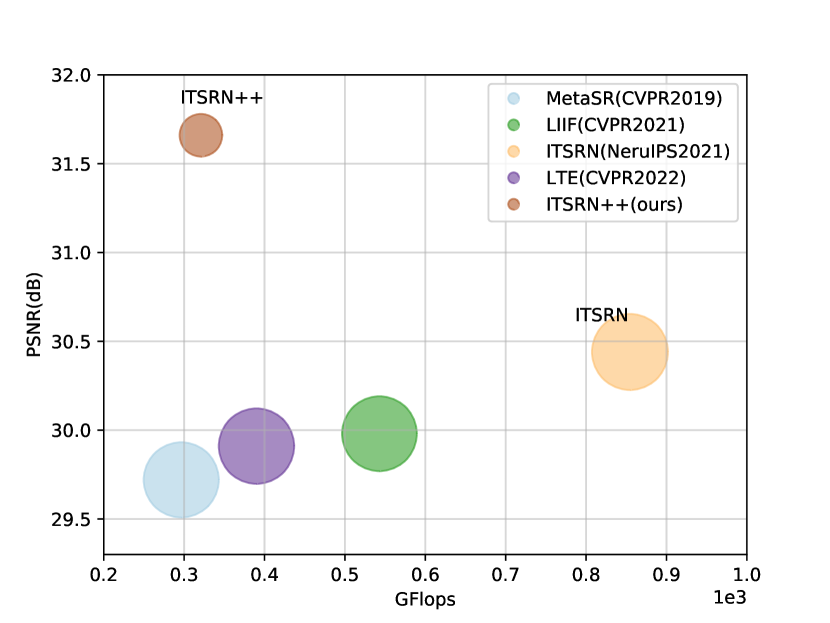
Figure 10: Computing complexity comparison. The PSNR results are evaluated on the SCI2K test set for $\times 4$ SR. The FLOPs are calculated with a $128\times 128$ input. The circle size indicates the number of parameters.

Figure 10 presents the performance versus the FLOPs of continuous SR methods. The number of parameters is represented by the size of the circle. A larger circle indicate a larger number of parameters. Compared with our previous version ITSRN, ITSRN++ saves about 60% FLOPs, but brings nearly 1 dB gain. Comparing to the MetaSR [12] and LIIF [13], our ITSRN++ has over 1 dB gain for $4\times$ SR.

5.3.2 Comparisons on Natural Image SR

Since most SR methods are evaluated on natural images, we further compare with state-of-the-arts on natural image SR. We re-train our method with DIV2K dataset [56] and evaluate on five benchmark datasets, i.e., Set5 [63], Set14 [64], BSDS100 [58], Urban100 [57] and Mange109 [65]. The compared methods are also trained on DIV2K and their results are directly quoted from the corresponding papers. Note that, the results for SwinIR-MetaSR and SwinIR-LIIF are realized by LTE [15].

The quantitative results are presented in Table VII. It can be observed that our ITSRN++ consistently outperforms existing methods on Urban100 and Mange109 datasets, since the images in the two datasets have many sharp edges (Urban100 is constructed by urban buildings and Mange109 is constructed by manga, one kind of screen contents). For example, for $\times 4$ SR, ITSRN++ outperforms SwinIR-LTE (the second best method) by 0.23 dB and 0.22 dB on Manga109 and Urban100, respectively. Meanwhile, our FLOPs are smaller than those of SwinIR-LTE. This demonstrates that the point-wise modulated upsampler and dual branch block are beneficial for sharp edge reconstruction. On the other three test sets, our method is comparable or slightly better than the compared methods. This verifies that our method can also work well for natural image SR. We also test on $\times 8$ SR to evaluate the continuity and robustness of our model. Note that, our ITSRN++ do not ”see” $\times 8$ pairs in training, but we still achieve the best performance in four benchmarks except Set5. For example, compared with SwinIR which is trained with $\times 8$ LR-HR pairs, our method still achieves 0.32 dB gain on Manga109. Compared with the second best method (SwinIR-LTE), our method achieves 0.16 dB gain.

Fig. 9 presents the visual comparison results for $\times 4$ SR on the Urban100 and Manga109 datasets. Our method accurately reconstructs parallel straight lines, grid patterns, and texts.

6 Conclusions and Limitation

In this work, we propose a better and stronger implicit transformer network for screen content image SR. With the proposed modulation based implicit transformer for upsampler and the enhanced explicit transformer for feature extraction, the proposed method achieves more than 1 dB gain against our previous conference version ITSRN. Experiments on four screen content image datasets and five benchmark natural image SR datasets demonstrate the superiority and generalizability of our method. Besides, a large high resolution screen content image dataset SCI2K is constructed, which will benefit the development of SCI SR methods.

We would like to point out that continuous SR methods usually consume more computing resources compared with fixed scale SR methods. Since there are MLPs in our upsampler, its computing complexity is higher than pixel shuffle based upsampler. In the future, we would like to optimize the upsampler to make it lighter.

References

- [1] W.-H. Peng, F. G. Walls, R. A. Cohen, J. Xu, J. Ostermann, A. MacInnis, and T. Lin, “Overview of screen content video coding: Technologies, standards, and beyond,” IEEE Journal on Emerging and Selected Topics in Circuits and Systems, vol. 6, no. 4, pp. 393–408, 2016.
- [2] B. Lim, S. Son, H. Kim, S. Nah, and K. Mu Lee, “Enhanced deep residual networks for single image super-resolution,” in IEEE Conference on Computer Vision and Pattern Recognition Workshops, 2017, pp. 136–144.
- [3] Y. Zhang, Y. Tian, Y. Kong, B. Zhong, and Y. Fu, “Residual dense network for image super-resolution,” in IEEE Conference on Computer Vision and Pattern Recognition, 2018, pp. 2472–2481.
- [4] Y. Zhang, K. Li, K. Li, L. Wang, B. Zhong, and Y. Fu, “Image super-resolution using very deep residual channel attention networks,” in European Conference on Computer Vision, 2018, pp. 286–301.
- [5] Y. Zhang, K. Li, K. Li, B. Zhong, and Y. Fu, “Residual non-local attention networks for image restoration,” arXiv preprint arXiv:1903.10082, 2019.
- [6] H. Chen, Y. Wang, T. Guo, C. Xu, Y. Deng, Z. Liu, S. Ma, C. Xu, C. Xu, and W. Gao, “Pre-trained image processing transformer,” in IEEE Conference on Computer Vision and Pattern Recognition, 2021, pp. 12 299–12 310.
- [7] Z. Li, J. Yang, Z. Liu, X. Yang, G. Jeon, and W. Wu, “Feedback network for image super-resolution,” in IEEE Conference on Computer Vision and Pattern Recognition, 2019, pp. 3867–3876.
- [8] J. Liang, J. Cao, G. Sun, K. Zhang, L. Van Gool, and R. Timofte, “SwinIR: Image restoration using swin transformer,” in IEEE Conference on International Conference on Computer Vision Workshops, 2021.
- [9] X. Kong, X. Liu, J. Gu, Y. Qiao, and C. Dong, “Reflash dropout in image super-resolution,” in Proceedings of the IEEE/CVF Conference on Computer Vision and Pattern Recognition, 2022, pp. 6002–6012.
- [10] Z. Lin, P. Garg, A. Banerjee, S. A. Magid, D. Sun, Y. Zhang, L. Van Gool, D. Wei, and H. Pfister, “Revisiting rcan: Improved training for image super-resolution,” arXiv preprint arXiv:2201.11279, 2022.
- [11] M. Wang, J. Xu, L. Zhang, J. Li, and S. Wang, “Super resolution for compressed screen content video,” in 2021 Data Compression Conference (DCC). IEEE, 2021, pp. 173–182.
- [12] X. Hu, H. Mu, X. Zhang, Z. Wang, T. Tan, and J. Sun, “Meta-sr: A magnification-arbitrary network for super-resolution,” in Proceedings of the IEEE/CVF conference on computer vision and pattern recognition, 2019, pp. 1575–1584.
- [13] Y. Chen, S. Liu, and X. Wang, “Learning continuous image representation with local implicit image function,” in Proceedings of the IEEE/CVF Conference on Computer Vision and Pattern Recognition, 2021, pp. 8628–8638.
- [14] J. Yang, S. Shen, H. Yue, and K. Li, “Implicit transformer network for screen content image continuous super-resolution,” Advances in Neural Information Processing Systems, vol. 34, 2021.
- [15] J. Lee and K. H. Jin, “Local texture estimator for implicit representation function,” arXiv preprint arXiv:2111.08918, 2021.
- [16] M. D. Zeiler, D. Krishnan, G. W. Taylor, and R. Fergus, “Deconvolutional networks,” in 2010 IEEE Computer Society Conference on computer vision and pattern recognition. IEEE, 2010, pp. 2528–2535.
- [17] W. Shi, J. Caballero, F. Huszár, J. Totz, A. P. Aitken, R. Bishop, D. Rueckert, and Z. Wang, “Real-time single image and video super-resolution using an efficient sub-pixel convolutional neural network,” in IEEE Conference on Computer Vision and Pattern Recognition, 2016, pp. 1874–1883.
- [18] B. Mildenhall, P. P. Srinivasan, M. Tancik, J. T. Barron, R. Ramamoorthi, and N. Ren, “Nerf: Representing scenes as neural radiance fields for view synthesis,” in European Conference on Computer Vision, 2020.
- [19] W.-S. Lai, J.-B. Huang, N. Ahuja, and M.-H. Yang, “Deep laplacian pyramid networks for fast and accurate super-resolution,” in Proceedings of the IEEE conference on computer vision and pattern recognition, 2017, pp. 624–632.
- [20] B. Niu, W. Wen, W. Ren, X. Zhang, L. Yang, S. Wang, K. Zhang, X. Cao, and H. Shen, “Single image super-resolution via a holistic attention network,” in European conference on computer vision. Springer, 2020, pp. 191–207.
- [21] T. Tong, G. Li, X. Liu, and Q. Gao, “Image super-resolution using dense skip connections,” in Proceedings of the IEEE international conference on computer vision, 2017, pp. 4799–4807.
- [22] Y. Mei, Y. Fan, and Y. Zhou, “Image super-resolution with non-local sparse attention,” in Proceedings of the IEEE/CVF Conference on Computer Vision and Pattern Recognition (CVPR), June 2021, pp. 3517–3526.
- [23] Y. Mei, Y. Fan, Y. Zhou, L. Huang, T. S. Huang, and H. Shi, “Image super-resolution with cross-scale non-local attention and exhaustive self-exemplars mining,” in Proceedings of the IEEE Conference on Computer Vision and Pattern Recognition (CVPR). IEEE, 2020.
- [24] B. Xia, Y. Hang, Y. Tian, W. Yang, Q. Liao, and J. Zhou, “Efficient non-local contrastive attention for image super-resolution,” 2022.
- [25] L. Wang, Y. Wang, Z. Lin, J. Yang, W. An, and Y. Guo, “Learning a single network for scale-arbitrary super-resolution,” in Proceedings of the IEEE/CVF International Conference on Computer Vision, 2021, pp. 4801–4810.
- [26] G. Huang, Z. Liu, L. van der Maaten, and K. Q. Weinberger, “Densely connected convolutional networks,” in Proceedings of the IEEE Conference on Computer Vision and Pattern Recognition, 2017.
- [27] G. Huang, Z. Liu, G. Pleiss, L. Van Der Maaten, and K. Weinberger, “Convolutional networks with dense connectivity,” IEEE Transactions on Pattern Analysis and Machine Intelligence, 2019.
- [28] J. Hu, L. Shen, and G. Sun, “Squeeze-and-excitation networks,” 2018.
- [29] A. Vaswani, N. Shazeer, N. Parmar, J. Uszkoreit, L. Jones, A. N. Gomez, Ł. Kaiser, and I. Polosukhin, “Attention is all you need,” Advances in neural information processing systems, vol. 30, 2017.
- [30] Z. Liu, Y. Lin, Y. Cao, H. Hu, Y. Wei, Z. Zhang, S. Lin, and B. Guo, “Swin transformer: Hierarchical vision transformer using shifted windows,” in Proceedings of the IEEE/CVF International Conference on Computer Vision, 2021, pp. 10 012–10 022.
- [31] Z. Chen and H. Zhang, “Learning implicit fields for generative shape modeling,” in Proceedings of the IEEE/CVF Conference on Computer Vision and Pattern Recognition, 2019, pp. 5939–5948.
- [32] M. Atzmon and Y. Lipman, “Sal: Sign agnostic learning of shapes from raw data,” in 2020 IEEE/CVF Conference on Computer Vision and Pattern Recognition (CVPR), 2020, pp. 2565–2574.
- [33] K. Genova, F. Cole, A. Sud, A. Sarna, and T. Funkhouser, “Local deep implicit functions for 3d shape,” in Proceedings of the IEEE/CVF Conference on Computer Vision and Pattern Recognition, 2020, pp. 4857–4866.
- [34] J. J. Park, P. Florence, J. Straub, R. Newcombe, and S. Lovegrove, “Deepsdf: Learning continuous signed distance functions for shape representation,” in Proceedings of the IEEE/CVF Conference on Computer Vision and Pattern Recognition, 2019, pp. 165–174.
- [35] D. Rebain, W. Jiang, S. Yazdani, K. Li, K. M. Yi, and A. Tagliasacchi, “Derf: Decomposed radiance fields.” arXiv preprint arXiv:2011.12490, 2020.
- [36] K. Zhang, G. Riegler, N. Snavely, and V. Koltun, “Nerf++: Analyzing and improving neural radiance fields,” arXiv preprint arXiv:2010.07492, 2020.
- [37] J. T. Barron, B. Mildenhall, M. Tancik, P. Hedman, R. Martin-Brualla, and P. P. Srinivasan, “Mip-nerf: A multiscale representation for anti-aliasing neural radiance fields,” in Proceedings of the IEEE/CVF International Conference on Computer Vision, 2021, pp. 5855–5864.
- [38] J. T. Barron, B. Mildenhall, D. Verbin, P. P. Srinivasan, and P. Hedman, “Mip-nerf 360: Unbounded anti-aliased neural radiance fields,” in Proceedings of the IEEE/CVF Conference on Computer Vision and Pattern Recognition, 2022, pp. 5470–5479.
- [39] L. Mescheder, M. Oechsle, M. Niemeyer, S. Nowozin, and A. Geiger, “Occupancy networks: Learning 3d reconstruction in function space,” in Proceedings of the IEEE/CVF Conference on Computer Vision and Pattern Recognition, 2019, pp. 4460–4470.
- [40] S. Peng, M. Niemeyer, L. M. Mescheder, M. Pollefeys, and A. Geiger, “Convolutional occupancy networks,” in ECCV (3), 2020, pp. 523–540.
- [41] S. Liu, X. Xu, S. Lei, and K. Jou, “Overview of hevc extensions on screen content coding,” APSIPA Transactions on Signal and Information Processing, vol. 4, 2015.
- [42] S. Wang, X. Zhang, X. Liu, J. Zhang, S. Ma, and W. Gao, “Utility-driven adaptive preprocessing for screen content video compression,” IEEE Transactions on Multimedia, vol. 19, no. 3, pp. 660–667, 2017.
- [43] W.-H. Peng, F. G. Walls, R. A. Cohen, J. Xu, J. Ostermann, A. MacInnis, and T. Lin, “Overview of screen content video coding: Technologies, standards, and beyond,” IEEE Journal on Emerging and Selected Topics in Circuits and Systems, vol. 6, no. 4, pp. 393–408, 2016.
- [44] T. Tang, L. Li, X. Wu, R. Chen, H. Li, G. Lu, and L. Cheng, “Tsa-scc: text semantic-aware screen content coding with ultra low bitrate,” IEEE Transactions on Image Processing, vol. 31, pp. 2463–2477, 2022.
- [45] M. Wang, Z. Xu, X. Liu, J. Xiong, and W. Xie, “Perceptually quasi-lossless compression of screen content data via visibility modeling and deep forecasting,” IEEE Transactions on Industrial Informatics, 2022.
- [46] H. Yang, Y. Fang, and W. Lin, “Perceptual quality assessment of screen content images,” IEEE Transactions on Image Processing, vol. 24, no. 11, pp. 4408–4421, 2015.
- [47] K. Gu, G. Zhai, W. Lin, X. Yang, and W. Zhang, “Learning a blind quality evaluation engine of screen content images,” Neurocomputing, vol. 196, pp. 140–149, 2016.
- [48] Z. Ni, L. Ma, H. Zeng, J. Chen, C. Cai, and K.-K. Ma, “Esim: Edge similarity for screen content image quality assessment,” IEEE Transactions on Image Processing, vol. 26, no. 10, pp. 4818–4831, 2017.
- [49] Z. Ni, L. Ma, H. Zeng, C. Cai, and K.-K. Ma, “Gradient direction for screen content image quality assessment,” IEEE Signal Processing Letters, vol. 23, no. 10, pp. 1394–1398, 2016.
- [50] X. Min, K. Gu, G. Zhai, X. Yang, W. Zhang, P. Le Callet, and C. W. Chen, “Screen content quality assessment: overview, benchmark, and beyond,” ACM Computing Surveys (CSUR), vol. 54, no. 9, pp. 1–36, 2021.
- [51] V. Sitzmann, J. Martel, A. Bergman, D. Lindell, and G. Wetzstein, “Implicit neural representations with periodic activation functions,” Advances in Neural Information Processing Systems, vol. 33, 2020.
- [52] M. Tancik, P. P. Srinivasan, B. Mildenhall, S. Fridovich-Keil, N. Raghavan, U. Singhal, R. Ramamoorthi, J. T. Barron, and R. Ng, “Fourier features let networks learn high frequency functions in low dimensional domains,” in Advances in Neural Information Processing Systems, vol. 33, 2020, pp. 7537–7547.
- [53] Q. Chen, Q. Wu, J. Wang, Q. Hu, T. Hu, E. Ding, J. Cheng, and J. Wang, “Mixformer: Mixing features across windows and dimensions,” in Proceedings of the IEEE/CVF Conference on Computer Vision and Pattern Recognition, 2022, pp. 5249–5259.
- [54] C. Si, W. Yu, P. Zhou, Y. Zhou, X. Wang, and S. Yan, “Inception transformer,” arXiv preprint arXiv:2205.12956, 2022.
- [55] X. Chen, X. Wang, J. Zhou, and C. Dong, “Activating more pixels in image super-resolution transformer,” arXiv preprint arXiv:2205.04437, 2022.
- [56] E. Agustsson and R. Timofte, “Ntire 2017 challenge on single image super-resolution: Dataset and study,” in Proceedings of the IEEE conference on computer vision and pattern recognition workshops, 2017, pp. 126–135.
- [57] J.-B. Huang, A. Singh, and N. Ahuja, “Single image super-resolution from transformed self-exemplars,” in Proceedings of the IEEE conference on computer vision and pattern recognition, 2015, pp. 5197–5206.
- [58] D. Martin, C. Fowlkes, D. Tal, and J. Malik, “A database of human segmented natural images and its application to evaluating segmentation algorithms and measuring ecological statistics,” in Proceedings Eighth IEEE International Conference on Computer Vision. ICCV 2001, vol. 2. IEEE, 2001, pp. 416–423.
- [59] M. Friend and M. Keplinger, “Reliability and validity of the computerized comprehension task (cct): data from american english and mexican spanish infants,” Journal of child language, vol. 35, no. 1, p. 77, 2008.
- [60] J. Gu and C. Dong, “Interpreting super-resolution networks with local attribution maps,” in Proceedings of the IEEE/CVF Conference on Computer Vision and Pattern Recognition, 2021, pp. 9199–9208.
- [61] X. Min, K. Ma, K. Gu, G. Zhai, Z. Wang, and W. Lin, “Unified blind quality assessment of compressed natural, graphic, and screen content images,” IEEE Transactions on Image Processing, vol. 26, no. 11, pp. 5462–5474, 2017.
- [62] S. Zhou, J. Zhang, W. Zuo, and C. C. Loy, “Cross-scale internal graph neural network for image super-resolution,” in Advances in Neural Information Processing Systems, 2020.
- [63] M. Bevilacqua, A. Roumy, C. Guillemot, and M. L. Alberi-Morel, “Low-complexity single-image super-resolution based on nonnegative neighbor embedding,” 2012.
- [64] R. Zeyde, M. Elad, and M. Protter, “On single image scale-up using sparse-representations,” in International conference on curves and surfaces. Springer, 2010, pp. 711–730.
- [65] Y. Matsui, K. Ito, Y. Aramaki, A. Fujimoto, T. Ogawa, T. Yamasaki, and K. Aizawa, “Sketch-based manga retrieval using manga109 dataset,” Multimedia Tools and Applications, vol. 76, no. 20, pp. 21 811–21 838, 2017.