Asymptotic control of the mean-squared error for Monte Carlo sensitivity index estimators in stochastic models

Abstract

In global sensitivity analysis for stochastic models, the Sobol’ sensitivity index is a ratio of polynomials in which each variable is an expectation of a function of a conditional expectation. The estimator is then based on nested Monte Carlo sampling where the sizes of the inner and outer loops correspond to the number of repetitions and explorations, respectively. Under some conditions, it was shown that the optimal rate of the mean squared error for estimating the expectation of a function of a conditional expectation by nested Monte Carlo sampling is of order the computational budget raised to the power -2/3. However, the control of the mean squared error for ratios of polynomials is more challenging. We show the convergence in quadratic mean of the Sobol’ index estimator. A bound is found that allows us to propose an allocation strategy based on a bias-variance trade-off. A practical algorithm that adapts to the model intrinsic randomness and exploits the knowledge of the optimal allocation is proposed and illustrated on numerical experiments.

Keywords: Stochastic model, global sensitivity analysis, Monte-Carlo method, mean-squared error, quadratic convergence.

1 Introduction

Sensitivity analysis (SA) provides useful insight into mathematical models. However, in SA, stochastic models are challenging. Indeed, such models include two sources of uncertainty: parameter uncertainty and intrinsic randomness. This intrinsic randomness is a collection of hidden random variables that can make challenging the definition of meaningful sensitivity indices and their efficient estimation.

Several methods have been introduced to deal with stochastic models. Apart from metamodel-based approach (Étoré et al., 2020; Jimenez et al., 2017; Fort et al., 2013; Zhu and Sudret, 2021), usual SA methods for stochastic models may be divided into about three approaches. The first approach, proposed by Hart et al. (2017), considers random Sobol’-Hoeffding decompositions (Sobol’, 1993) of stochastic model outputs and defines sensitivity indices of such models as expectations of the resulting random Sobol’ indices. The second approach focuses on deterministic quantities of interest (QoIs) such as conditional expectations or conditional variances (Courcoul et al., 2011; Mazo, 2021). By conditioning with respect to the uncertain parameters, the aim is to smooth the intrinsic randomness out and hence to deal with quantities under the form of deterministic functions of the uncertain parameters only, so that SA methods for deterministic models can be applied. The third approach includes recently developed methods (Fort et al. (2021); Gamboa et al. (2021), da Veiga (2021)) that see stochastic output models as deterministic function with values in probability distribution spaces. Various sensitivity indices are defined on such spaces in order to measure contributions of uncertain parameters.

For all these approaches, it appears that not only should the model be evaluated at many points in the input space (it is said that the input space is explored), but also the model should be repeated at each of those explorations to estimate conditional expectations. In the first approach, these repetitions are performed when approximating the expectations of the random Sobol’ indices. In the second and third approaches, model outputs are repeated when estimating the QoIs and the probability distributions, respectively. Therefore, the larger the number of explorations and the number of repetitions, the more accurate the sensitivity index estimators. This leads to large numbers of runs of the model. However, in practice, models could be complex and a run could have a high computational cost so that computational issue could rise very quickly.

Therefore, the study of the choice of a number of explorations and a number of repetitions under the constraint of a computational cost or that of the precision of estimations, takes more and more importance beyond the sensitivity analysis but more globally in the fields which are interested in the stochastic simulators. It can be mentioned the works of Chen and Zhou (2014, 2017) which proposes various strategies of sequential design based on the Integrative Mean Squared Error (IMSE) for stochastic kriging. More recently still with metamodels based on Gaussian processes, Binois et al. (2018, 2019) explored different methods for optimal design also using IMSE criteria.

In Mazo (2021), the author studied this problem for estimation of sensitivity indices for stochastic models. In that paper, two QoIs were considered: the exact model output and its conditional expectation with respect to the uncertain parameters. Depending on the QoI, two types of Sobol’ indices were defined and the so-called pick-freeze estimators (Gamboa et al. (2016)) were used. Those estimators are based on a double (or nested) Monte-Carlo sampling scheme and require the choice of the number of explorations, $n$, and the number of repetitions, $m$. Such procedure is the so-called Nested Monte Carlo. To better estimate such indices without increasing the computation cost, Mazo (2021) supposed that the total number of runs of the model is fixed and then proposed under such constraint a choice of $n$ and $m$ based on the minimization of some bound of the so-called mean ranking error (MRE) of the estimators. This error measures the gap between the ranks of the theoretical indices and those of the estimators. However, a small MRE does not necessarily imply that estimations are close to their theoretical values.

Accurate and efficient estimation of Sobol’ indices is a major concern in SA . This is linked to the problem of accurately estimating expectation of functions of conditional moments, which is a problem that arises in wider framework than SA. Many studies have been conducted to address this issue. In global sensitivity analysis, da Veiga and Gamboa (2013) addressed the problem with a semi-parametric estimation approach (see also da Veiga et al. (2017)) in the case of deterministic models while Mycek and De Lozzo (2019) proposed methods based on Multilevel Monte-Carlo. In the case of metamodel based SA, Janon et al. (2014); Panin (2021) studied the risk of estimators and provide error bounds. Regarding stochastic models, Castellan et al. (2020) discussed the accurate non-parametric estimation of first-order Sobol’ indices for bounded stochastic models by relying on wavelet-based estimator approach. More generally, beyond SA, Rainforth et al. (2018) studied the nested Monte Carlo and its computational cost. Giles and Haji-Ali (2019); Giorgi et al. (2020) discussed efficiency and convergence rates of Multilevel nested Monte-Carlo. Control of the mean squared error (MSE) of Sobol index estimators in various frameworks was discussed in the literature (Solís, 2019; Castellan et al., 2020). However, the results appear to be incomplete, since the conditions under which they may hold are not provided.

In this paper, we consider deterministic QoIs that are under the form of conditional expectations of some transformations of the stochastic model output with respect to the inputs. This class of QoIs includes the much used conditional expectation and conditional variance of the stochastic model output with respect to the inputs. We focus on variance-based indices such as first-order and total Sobol’ indices for inputs or groups of inputs. The estimation of those indices is based on the pick-freeze method by using $n$ explorations of the input space and $m$ model repetitions. We study MSEs of sensitivity index estimators and propose tractable upper bounds that depend on both $n$ and $m$. Then, under the constraint that $n=T^{1-\eta}$ and $m=T^{\eta}$, $\eta\in[0,1)$, with $T\to\infty$, the bias-variance trade-off is studied using those upper-bounds and the optimal allocation parameter $\eta$ is deduced.

The main interest of this work lies in three points. First, up to some mild assumptions on the model outputs, pick-freeze estimators of first-order and total Sobol’ indices are shown to converge in quadratic means. (We note that a byproduct of this result is the convergence in quadratic mean of the “usual” Sobol’ index estimators for deterministic models.) Second, the scope of this study is large. It takes into account a large class of QoIs of stochastic model outputs and it includes two widely-used sensitivity indices. Finally, algorithms are provided for practical implementation of our results. These algorithms are expected to give better estimations of Sobol’ indices.

This paper is organized as follows. Section 2 presents the general framework of stochastic models and QoI-based sensitivity indices. In Section 3, the MSE of a general class of estimators that contains our sensitivity indices is considered and its asymptotic behavior presented. Section 4 is dedicated to studying the MSE of some variance-based sensitivity indices. The bias-variance trade-off is discussed and the optimal allocation for $m$ and $n$ is given here. A practical procedure is implemented through two algorithms and illustrated on two toy models in Section 5. A conclusion closes the paper.

2 Sensitivity index estimators

A stochastic model with inputs $\mathbf{X}=(X_{1},\dots,X_{p})\in\mathbb{R}^{p}$ and output $Y\in\mathbb{R}$ is modeled as a function $f$ of $\mathbf{X}$ and some collection of random variables, denoted by $Z$, independent of $\mathbf{X}$ such that

$$Y=f\left(\mathbf{X},Z\right).$$ (1)

The stochasticity of the model originates from $Z$ since the output of the model evaluated at an input $\mathbf{X}=x$ is a random variable $f(x,Z)$. The distribution of $Z$ is generally unknown.

In the context of SA, a way to deal with stochastic models consists in carrying out SA for deterministic models given by deterministic QoIs. This allows to switch from a stochastic model to some deterministic models for which many SA methods are studied in the literature.

We consider QoIs of the form

$$Q(\mathbf{X})=\mathbb{E}\left[\varphi(\mathbf{X},Z)\mid\mathbf{X}\right],$$ (2)

where $\varphi(\mathbf{X},Z)$ is a function of $\mathbf{X}$ and $Z$. For instance, if $\varphi=f$ then $Q(\mathbf{X})$ is the conditional expectation of the model and if $\varphi(\mathbf{X},Z)=\left(f(\mathbf{X},Z)-\mathbb{E}\left[f(\mathbf{X},Z)\mid\mathbf{X}\right]\right)^{2}$ then $Q(\mathbf{X})$ is the conditional variance, two common choices in practice.

If $u$ is a subset of $\{1,\dots,p\}$, denote by $\mathbf{X}_{u}$ the group of inputs $\{X_{i},i\in u\}$ and $\mathbf{X}_{\sim u}$ the group of inputs $\{X_{i},i\not\in u\}$. The Sobol’ and total indices of the input vector $\mathbf{X}_{u}$ with respect to the function $Q$ are defined as

$$S_{u} =\frac{\text{Var}\left(\mathbb{E}\left[Q(\mathbf{X})\mid\mathbf{X}_{u}\right]\right)}{\text{Var}\left(Q(\mathbf{X})\right)}$$ (3)

$$T_{u} =1-\frac{\text{Var}\left(\mathbb{E}\left[Q(\mathbf{X})\mid\mathbf{X}_{\sim u}\right]\right)}{\text{Var}\left(Q(\mathbf{X})\right)}=1-S_{\sim u}.$$ (4)

The sensitivity index $S_{u}$ (and hence $T_{u}$) can be expressed in terms of a function $g$ linking the components of some parameter vector. Let $\widetilde{\mathbf{X}}$ be an independent copy of $\mathbf{X}$, independent of $Z$. Denote by $\widetilde{\mathbf{X}}_{\sim u}$ the subvector of $\widetilde{\mathbf{X}}$ whose components are those of $\widetilde{\mathbf{X}}$ not indexed by $u$. (For instance, if $p=4$ and $u=\{1,4\}$ then $\widetilde{\mathbf{X}}_{\sim u}=(\widetilde{X}_{2},\widetilde{X}_{3})$.) If $\theta=(\theta_{1},\theta_{2},\theta_{3})$ with $\theta_{1}=\mathbb{E}(Q(\mathbf{X})^{2})$, $\theta_{2}=\mathbb{E}(Q(\mathbf{X}))$ and $\theta_{3}=\mathbb{E}(\mathbb{E}\left[Q(\mathbf{X})\mid\mathbf{X}_{u}\right]^{2})=\mathbb{E}(Q(\mathbf{X})Q(\widetilde{\mathbf{X}}_{\sim u},\mathbf{X}_{u}))=\mathbb{E}(Q(\mathbf{X}_{\sim u},\mathbf{X}_{u})Q(\widetilde{\mathbf{X}}_{\sim u},\mathbf{X}_{u}))$ then

$$S_{u}=g(\theta)=\frac{\theta_{3}-\theta_{2}^{2}}{\theta_{1}-\theta_{2}^{2}}.$$

An estimator of $S_{u}$ is built by the method-of-moments (pick-freeze procedure). Let $\{\mathbf{X}^{(i)};i=1,\dots,n\}$ and $\{\widetilde{\mathbf{X}}^{(i)};i=1,\dots,n\}$ be independent Monte Carlo samples from the law of $\mathbf{X}$. For each $i$, denote by $\mathbf{X}_{u}^{(i)}$ the subvector of $\mathbf{X}^{(i)}$ whose components are those of $\mathbf{X}^{(i)}$ indexed by $u$. Likewise, denote by $\mathbf{X}_{\sim u}^{(i)}$ the subvector of $\mathbf{X}^{(i)}$ whose components are those of $\mathbf{X}^{(i)}$ not indexed by $u$, and denote by $\widetilde{\mathbf{X}}_{\sim u}^{(i)}$ the subvector of $\widetilde{\mathbf{X}}^{(i)}$ whose components are those of $\widetilde{\mathbf{X}}^{(i)}$ not indexed by $u$. An estimator of $S_{u}$ is given by

$$\widehat{S}_{u}=g(\widehat{\theta})=\frac{\widehat{\theta}_{3}-\widehat{\theta}_{2}^{2}}{\widehat{\theta}_{1}-\widehat{\theta}_{2}^{2}}$$

where

$$\left.\begin{array}[]{rcl}\widehat{\theta}_{1}&=&\frac{1}{n}\sum_{i=1}^{n}\widehat{Q}_{m}(\mathbf{X}^{(i)})^{2}\\ \widehat{\theta}_{2}&=&\frac{1}{n}\sum_{i=1}^{n}\widehat{Q}_{m}(\mathbf{X}^{(i)})\\ \widehat{\theta}_{3}&=&\frac{1}{n}\sum_{i=1}^{n}\widehat{Q}_{m}(\mathbf{X}^{(i)})\widetilde{Q}_{m}(\widetilde{\mathbf{X}}^{(i)}_{\sim u},\mathbf{X}^{(i)}_{u})\\ \end{array}\right\}$$ (5)

and

$$\widehat{Q}_{m}(\mathbf{X}^{(i)}) = \frac{1}{m}\sum_{k=1}^{m}\varphi\left(\mathbf{X}^{(i)},Z^{(i,k)}\right)$$

$$\widetilde{Q}_{m}(\widetilde{\mathbf{X}}^{(i)}_{\sim u},\mathbf{X}^{(i)}_{u}) = \frac{1}{m}\sum_{k=1}^{m}\varphi(\widetilde{\mathbf{X}}_{\sim u}^{(i)},\mathbf{X}_{u}^{(i)},\widetilde{Z}^{(i,k)});$$

here the objects $\{Z^{(i,k)},\widetilde{Z}^{(i,k)};k=1,\cdots,m;i=1,\cdots,n\}$, are independent and identically distributed random variables, independent of $\{\mathbf{X}^{(i)},\widetilde{\mathbf{X}}^{(i)};i=1,\dots,n\}$, representing the randomness of the user’s model. For more details, see Mazo (2021).

The estimator $\widehat{S}_{u}$ may be asymptotically biased , depending on the rate at which $m$, the number of repetitions, increases with respect to $n$, the number of explorations. It was shown in Mazo (2021) that, if $m$ is fixed, then

$$\sqrt{n}\left(\widehat{S}_{u}-S_{u}\left[1-\frac{\operatorname{E}\operatorname{Var}(\varphi(\mathbf{X},Z)|\mathbf{X})}{\operatorname{E}\operatorname{Var}(\varphi(\mathbf{X},Z)|\mathbf{X})+m\operatorname{Var}\operatorname{E}(\varphi(\mathbf{X},Z)|\mathbf{X})}\right]\right)$$

converges to a centered normal distribution with some variance $\sigma_{m}^{2}$ depending on $m$. To get rid of the bias, it is needed that $m\to\infty$ such that $\sqrt{n}/m\to 0$, in which case $\sqrt{n}(\widehat{S}_{u}-S_{u})$ goes to a centered normal distribution with variance $\lim_{m\to\infty}\sigma_{m}^{2}$.

The statistical performance of the estimator $\widehat{S}_{u}$ goes hand in hand with the computation effort one is ready to spend. The computation of $\widehat{S}_{u}$ requires a number of model evaluations proportional to $mn$. Given a fixed number of evaluations—and hence $mn$ is fixed—it is of interest to find the couple $(m,n)$ that most increases the estimator’s performance. In Mazo (2021), a bound on an error that penalizes bad rankings of the sensitivity indices $S_{1},\dots,S_{p}$ was minimized, leading to a theoretically-guided choice for $m$ and $n$. However, it is more natural to consider the MSE $\mathbb{E}((\widehat{S}_{u}-S_{u})^{2})$ as the quantity to be controlled.

3 Mean-squared error control of smooth functions

In this section, we study the MSEs of some estimators and give bounds and a rate of convergence. The aim is to characterize a class of estimators that include variance-based sensitivity index estimators and then to define conditions under which their MSEs admit tractable upper bounds and convergence rates.

For sake of generality, let us consider a convex domain $\mathcal{D}\subset\mathbb{R}^{q}$ with $q\geq 1$. For each $m\in\mathbb{N}^{*}$, let $\widetilde{\theta}_{m}^{(1)},\cdots\widetilde{\theta}_{m}^{(n)}$ be $n$ i.i.d. random vectors whose common probability distribution depends only on $m$. Denote $\mu_{m}=\mathbb{E}(\widetilde{\theta}_{m}^{(1)})$ and
$\Sigma_{m}=\mathbb{E}\left((\widetilde{\theta}_{m}^{(1)}-\mu_{m})(\widetilde{\theta}_{m}^{(1)}-\mu_{m})^{\top}\right)$. Let $\theta\in\mathcal{D}$ and assume

$$\widehat{\theta}^{(n,m)}=\frac{1}{n}\sum_{i=1}^{n}\widetilde{\theta}_{m}^{(i)}$$ (6)

is an estimator of $\theta$. Let $b_{m}$ be the bias of $\widehat{\theta}^{(n,m)}$. Thus: $b_{m}=\mu_{m}-\theta$. For the sake of simplicity, hereafter, $\widehat{\theta}^{(n,m)}$ is denoted $\widehat{\theta}$. If $m$ is fixed then $\mathbb{E}(\widehat{\theta})=\mu_{m}\neq\theta$ as soon as $b_{m}$ is non-null. In particular, estimator $\widehat{\theta}$ belongs to the class of Nested Monte-Carlo estimators  if for $i=1,\cdots,n$, $\widetilde{\theta}_{m}^{(i)}$ are under the form

$$\widetilde{\theta}_{m}^{(i)}=\phi\left(\frac{1}{m}\sum_{k=1}^{m}\widetilde{\eta}^{(i,k)}\right),$$ (7)

where $\phi$ is some measurable function with values on $\mathcal{D}$ and $\{\widetilde{\eta}^{(i,k)};i=1,\cdots,n;k=1,\cdots,m\}$ is an array of identically distributed random vectors such that $\{\widetilde{\eta}^{(i,k)},k=1,\cdots,m\}$ and $\{\widetilde{\eta}^{(j,k)},k=1,\cdots,m\}$ are mutually independent as soon as $i\neq j$. The MSE of $\widehat{\theta}$ is given by $\mathbb{E}\,\|\widehat{\theta}-\theta\|^{2}$ and then, the variance bias decomposition yields:

$$\mathbb{E}\,\|\widehat{\theta}-\theta\|^{2} =\frac{1}{n}\text{Trace}\left(\Sigma_{m}\right)+\|b_{m}\|^{2}.$$ (8)

Make the following assumption:

Assumption 1.

$b_{m}\to 0$ and $\Sigma_{m}\to\Sigma$ as $m\to+\infty$.

Under Assumption 1, it holds that $\lim_{n,m\to+\infty}\mathbb{E}\,\|\widehat{\theta}-\theta\|^{2}=0$ and thereby $\widehat{\theta}$ converges in quadratic means to $\theta$. Mazo (2021) showed that Assumption 1 is satisfied by Sobol’ index estimators introduced in Section 2. More generally, this assumption is fulfilled in the case Nested Monte Carlo estimators provided that $\theta=\mathbb{E}\phi(\widetilde{\eta})$, with $\widetilde{\eta}$ the limit (provided it exists) of $\sum_{k=1}^{m}\widetilde{\eta}^{(1,k)}/m$, and that the function $\phi$ in Equation (7) has good properties such as boundedness and smoothness (Giorgi et al., 2017; Rainforth et al., 2018).

The form of the MSE in Equation (8) allows to control this error through the choice of $n$ and $m$. Indeed, this enables to show convergence, to obtain convergence rates and to study optimal convergence strategies. For instance, in the framework of Nested Monte Carlo estimators, Hong and Juneja (2009) showed that for a real-valued function $\phi$ (introduced in (7)) at least third differentiable such that the third derivative is uniformly bounded, the MSE defined in (8) is of order $O(1/n+1/m^{2})$ and they deduced that the optimal convergence rate is $O(T^{-2/3})$ if $T=mn$ denotes the computational effort. Thus, it is useful to have either the mean-squared error or at least an upper bound of this error under the form in (8).

Now, given a non-constant function $g:\mathcal{D}\rightarrow\mathbb{R}$, assume that $\widehat{\theta}$ is mapped to $g(\widehat{\theta})$ so that $g(\widehat{\theta})$ converges in probability to $g(\theta)$ as $n,m\to\infty$. Therefore, the main concern is to know if, as $\widehat{\theta}$, the MSE of $g(\widehat{\theta})$, i.e. $\mathbb{E}\,(g(\widehat{\theta})-g(\theta))^{2}$ converges to 0, or if it admits an upper bound under the form in (8) that converges to 0 as $n,m\to\infty$. Introducing $g$ makes the study of the related MSE more challenging than the usual cases one could deal with, especially in the Nested Monte Carlo estimator framework (Giles, 2018; Giorgi et al., 2020). The obstacles to obtaining such upper bound for $\mathbb{E}\,(g(\widehat{\theta})-g(\theta))^{2}$ are multiple and involve both $\widehat{\theta}$ and $g$: issues related to boundedness or smoothness of $g$, or to the probability distribution of $\widehat{\theta}$ and its support, etc. Hence, responses to the main concern depend generally on both $\widehat{\theta}$ and $g$. For instance, assume $g$ is linear or more generally $g$ is Lipschitz continuous, then there exists an constant $L$ such that $\left|g(x^{\prime})-g(x)\right|\leq L\|x^{\prime}-x\|$. Thus:

$$\mathbb{E}\,\left(g(\widehat{\theta})-g(\theta)\right)^{2}\leq L^{2}\mathbb{E}\,\|\widehat{\theta}-\theta\|^{2},$$

and thereby such MSE admits upper bound of the form in (8).

However, it can be difficult to get an exact upper bound in this form. Very often, in practice, the function $g$ does not have good enough properties to obtain an exact bound. In this case, one could look for an approximate bound of the form (8), i.e. which is the sum of a quantity of the form (8) and a certain quantity negligible when $n,m$ go to infinity. For example, let $g$ be a twice continuously differentiable such that its Hessian matrix denoted $\nabla^{2}g$ is uniformly bounded. Then, up to existence of some moments of $\widehat{\theta}$, and combining Taylor-Lagrange expansion and convexity inequality yields:

$$\mathbb{E}\,\left(g(\widehat{\theta})-g(\theta)\right)^{2}\leq 2\mathbb{E}\left(\nabla g(\mu_{m})^{\top}\left(\widehat{\theta}-\mu_{m}\right)\right)^{2}+2\left(g(\mu_{m})-g(\theta)\right)^{2}\\ +O\left(\mathbb{E}\|\widehat{\theta}-\mu_{m}\|^{4}\right).$$

Thus, the MSE of $g(\widehat{\theta})$ admits an upper bound. In addition, assume that the following condition is satisfied:

Assumption 2.

As $n,m\to\infty$, it holds that:

$$\frac{\mathbb{E}\left(\|\widehat{\theta}-\mu_{m}\|^{8}\right)}{\left(\mathbb{E}\left(\nabla g\left(\mu_{m}\right)^{\top}\left(\widehat{\theta}-\mu_{m}\right)\right)^{2}\right)^{2}}=o(1).$$

Under Assumption 2, it appears that:

$$\mathbb{E}\,\left(g(\widehat{\theta})-g(\theta)\right)^{2}\leq 2(1+o(1))\mathbb{E}\left(\nabla g(\mu_{m})^{\top}\left(\widehat{\theta}-\mu_{m}\right)\right)^{2}+2\left(g(\mu_{m})-g(\theta)\right)^{2}$$ (9)

and therefore the $\mathbb{E}\,(g(\widehat{\theta})-g(\theta))^{2}$ has approximately the form in (8) as $n,m\to\infty$. Though, the uniform boundedness of $\nabla^{2}g$ is a very strong condition. A way to weaken such a condition consists in having:

$$\sup_{\lambda\in(0,1)}\mathbb{E}\left(\|\nabla^{2}g\left(\lambda\widehat{\theta}+(1-\lambda)\mu_{m}\right)\|_{F}^{4}\right)=O(1)\quad\text{ as }n,m\to\infty,$$ (10)

where $\|\cdot\|_{F}$ denotes the Frobenius norm. Under condition in (10), the approximate decomposition (9) of the MSE into a sum of variance and squared bias holds. Therefore, the bias-variance tradeoff problem can be likely addressed more easily since the terms of the upper bound are more tractable. Also, a well-informed choice for the $(n,m)$ can be likely found to reduce the MSE.

Relying on Rosenthal inequality (Yuan and Li, 2015) and Marcinkiewicz–Zygmund inequality (Marcinkiewicz and Zygmund, 1937), Assumption 2 can be satisfied up to existence of moments of $\widehat{\theta}$. However, once again, even the condition provided in Equation (10) is still strong in general since this could impose a strong constraint on the probability distribution of $\widehat{\theta}$ which is generally unknown. For instance, in the case of Sobol’ index estimators defined in Section 2, condition (10) comes down to provide upper bounds for quantities under the form $\mathbb{E}[(\widehat{\theta}_{1}-\widehat{\theta}_{2}^{2})^{-\alpha}]$ with $\alpha>0$ whereas the probability distribution of $\widehat{\theta}_{1}-\widehat{\theta}_{2}^{2}$ is unknown and even the existence of such quantities is not guaranteed.

Faced with this issue, we propose a weaker condition than the one in Equation (10), which relaxes a little more the constraint on $\widehat{\theta}$. The idea is to introduce a "slight perturbation" $g_{h}$ of the function $g$ so that the condition of Equation (10) holds with $g=g_{h}$ and $\lim_{h\to 0}g_{h}(x)=g(x)$ pointwise. The advantage of having such a family of functions is that $\mathbb{E}(g_{h}(\widehat{\theta})-g_{h}(\theta))^{2}$, the “perturbed MSE”, could be bounded with an approximate upper bound in the form of Equation (9) with $g=g_{h}$. But the counterpart is that to control the “true” MSE, we also need to control $\Delta_{n,m}(h):=\mathbb{E}(g(\widehat{\theta})-g_{h}(\widehat{\theta}))^{2}$ which measures the distance between the “true” estimator $g(\widehat{\theta})$ and its modified version $g_{h}(\widehat{\theta})$. Thus, the difficulty is to find such a family for which this gap $\Delta_{n,m}(h)$ can also be controlled.

Let us fix $\mathbf{u}\in\mathbb{R}^{q}$ such that $\|\mathbf{u}\|=1$ and for all $x\in\mathcal{D}$, $x+h\mathbf{u}\in\mathcal{D}$ for any $h\in(0,1)$. Henceforth, we shall focus on the family defined by functions $g_{h}(x)=g(x+h\mathbf{u})$ which enables to control $\Delta_{n,m}(h)$ under Assumption 3 as $n,m\to\infty$.

Assumption 3.

There exists a constant $C$ independent of $h$ such that, for all $h\in(0,1)$:

$$\limsup_{n,m\rightarrow\infty}\sup_{\lambda\in[0,1]}\mathbb{E}\left(\|\nabla^{2}g(\lambda\hat{\theta}+(1-\lambda)\mu_{m}+h\mathbf{u})\|_{F}^{4}\right)\leq C.$$

Introducing translations $x\mapsto x+h\mathbf{u}$ can be thought as a way to "transport" the original estimator $\widehat{\theta}$ to regions of $\mathcal{D}$ where control of moments of $g(\widehat{\theta})$ is possible without additional conditions on $\widehat{\theta}$. Concretely, the goal of Assumption 3 is to “get away” from certain regions of the parameter space where the Hessian of $g$ may explode. Notice that the supremum over $\lambda$ is taken over the closed interval $[0,1]$. The choice of $h$ affects the approximation for the bound, as shown in Theorem 1. Recall that $\Delta_{n,m}(h):=\mathbb{E}\left(g(\widehat{\theta})-g(\widehat{\theta}+h\mathbf{u})\right)^{2}$ and let $V_{n,m}(h):=\mathbb{E}(\nabla g\left(\mu_{m}+h\mathbf{u}\right)^{\top}(\widehat{\theta}-\mu_{m}))^{2}$ and $B_{m}(h):=g\left(\mu_{m}+h\mathbf{u}\right)-g(\theta)$.

Theorem 1.

Under Assumptions 1, 2 and 3, there exists $\tilde{C}>0$ independent of $h$ such that for every $h\in(0,1)$:

$$\mathbb{E}\left(g(\widehat{\theta})-g(\theta)\right)^{2}\leq 3\left(1+p_{n,m}(h)\right)\left(\Delta_{n,m}(h)+V_{n,m}(h)+B_{m}(h)^{2}\right),$$ (11)

where $\limsup_{n,m\to\infty}p_{n,m}(h)=0$ and

$$\Delta_{n,m}(h)\leq\tilde{p}_{n,m}(h)h^{2},$$ (12)

where $\limsup_{n,m\to\infty}\tilde{p}_{n,m}(h)\leq\tilde{C}$.

Theorem 1 is the analog of (9), except that a term $\Delta_{n,m}(h)$ has appeared to control the gap between $g(\widehat{\theta}+h\mathbf{u})$ and $g(\widehat{\theta})$. The quantity $V_{n,m}(h)+B_{m}(h)^{2}$ can be rewritten to make the bias-variance trade-off appear. Indeed, $V_{n,m}(h)=n^{-1}\nabla g(\mu_{m}+h\mathbf{u})^{\top}\Sigma_{m}\nabla g(\mu_{m}+h\mathbf{u})$, which is of order $O(n^{-1})$ as $n,m\to\infty$, regardless of $h$. Moreover, we have $B_{m}(h)^{2}=((b_{m}+h\mathbf{u})^{\top}\nabla g(\overline{\theta}_{n,m}))^{2}$ for some $\overline{\theta}_{n,m}$ lying between $\theta$ and $\theta+b_{m}+h\mathbf{u}$, and hence $B_{m}(h)^{2}$ is bounded by $(\|b_{m}\|+h^{2})$ times some universal constant. Therefore, up to a universal multiplicative constant, it holds that $\Delta_{n,m}(h)+V_{n,m}(h)+B_{m}(h)^{2}$ is bounded by $h^{2}(\tilde{p}_{n,m}(h)+1)+1/n+\|b_{m}\|^{2}$, where $1/n+\|b_{m}\|^{2}$ represents the bias-variance tradeoff, which is similar to (8).

Letting $n,m\to\infty$ and then $h\to 0$ in (11), the convergence of the MSE can be shown, as stated in Corollary 1.

Corollary 1.

Under the conditions of Theorem 1, it holds that:

$$\lim_{n,m\to\infty}\mathbb{E}\left(g(\widehat{\theta})-g(\theta)\right)^{2}=0.$$

4 Application to sensitivity index estimators

This section aims at studying the MSE of estimators of Sobol’ indices introduced in Section 2. Let $\widehat{\theta}=(\widehat{\theta}_{1},\widehat{\theta}_{2},\widehat{\theta}_{3})$ be as in (5) and (6), where $\widehat{\theta}^{(i)}_{m}=(\widehat{\theta}_{m1}^{(i)},\widehat{\theta}_{m2}^{(i)},\widehat{\theta}_{m3}^{(i)})=(\widehat{Q}_{m}(\mathbf{X}^{(i)})^{2},\widehat{Q}_{m}(\mathbf{X}^{(i)}),\widehat{Q}_{m}(\mathbf{X}^{(i)})\widetilde{Q}_{m}(\widetilde{\mathbf{X}}^{(i)}_{\sim u},\mathbf{X}^{(i)}_{u})$. Recall that $\theta_{1}=\mathbb{E}(Q(\mathbf{X})^{2})$, $\theta_{2}=\mathbb{E}(Q(\mathbf{X}))$, $\theta_{3}=\mathbb{E}(\mathbb{E}\left[Q(\mathbf{X})\mid\mathbf{X}_{u}\right]^{2})=\mathbb{E}(Q(\mathbf{X})Q(\widetilde{\mathbf{X}}_{\sim u},\mathbf{X}_{u}))$, so that
$\mu_{m}=(\mu_{m1},\mu_{m2},\mu_{m3})=(\theta_{1}+b_{m1},\theta_{2}+b_{m2},\theta_{3}+b_{m3})$ and $b_{m}=(b_{m1},b_{m2},b_{m3})=(\mathbb{E}\text{Var}\left[\varphi(\mathbf{X},Z)\mid\mathbf{X}\right]/m,0,0)$. Recall that the function

$$g:(x_{1},x_{2},x_{3})\mapsto(x_{3}-x_{2}^{2})/(x_{1}-x_{2}^{2})$$ (13)

is a twice-continuously differentiable function over its definition domain. But unfortunately, $g$ is unbounded. The form of such a function makes the study of the MSE of Monte Carlo based Sobol index estimators almost impossible unless strong conditions are imposed on the output distribution of the model. This could explain why until now, to our knowledge, there is almost no study of the quadratic convergence of such estimators. The approach introduced in Section 3 allows to bypass the unbounded issue and thus, to establish the quadratic convergence of these estimators and to provide an approximate bound from which a strategy for optimizing convergence rate of the MSE is developed. Throughout this section, it is assumed that $\mathbb{E}\left(Q(\mathbf{X})^{16}\right)<+\infty$.

4.1 Control of the MSE

In order to provide an upper bound for $\mathbb{E}(g(\widehat{\theta})-g(\theta))^{2}$ as in Theorem 1, it is necessary to fulfill Assumption 1, 2 and 3. Assumption 1 is trivially satisfied. Since the estimator $\widehat{\theta}$ is an empirical mean of i.i.d. random vectors, we can show that Assumption 2 is satisfied—see Theorem 2.

Theorem 2.

In the context of Section 4 with $g$ given by (13), Assumption 2 is satisfied.

To check Assumption 3, we need to find a direction $\mathbf{u}$ that satisfies the required properties.

Theorem 3.

If $\mathbf{u}=(1,0,0)$, then, under the conditions of Theorem 1, Assumption 3 holds. Therefore, there is a constant $\bar{C}$ independent of $h$ such that, for every $h\in(0,1)$,

$$\mathbb{E}\left(g(\widehat{\theta})-g(\theta)\right)^{2}\leq\bar{p}_{n,m}(h)\left(\left(\frac{1}{n}+\left(\frac{\mathbb{E}\left(\text{Var}\left[\varphi(\mathbf{X},Z)\mid\mathbf{X}\right]\right)}{m}\right)^{2}\right)+h^{2}\bar{p}^{\prime}_{n,m}(h)\right),$$

where the supremum limits of $\bar{p}_{n,m}(h)$ and $\bar{p}^{\prime}_{n,m}(h)$ as $n,m\to\infty$ are less than $\bar{C}$.

Theorem 3 provides a bound for the MSE of the pick-freeze estimator $g(\widehat{\theta})$ of Sobol’ indices. This result is also valid in the deterministic framework, in which $\mathbb{E}\left(\text{Var}\left[\varphi(\mathbf{X},Z)\mid\mathbf{X}\right]\right)=0$. To the best of our knowledge, the convergence in quadratic mean of Sobol index estimators was not obtained in the literature yet, in both the deterministic and stochastic frameworks. This result is given in Corollary 2.

Corollary 2.

Under the conditions of Theorem 2, we have $\lim_{n,m\to\infty}\mathbb{E}(g(\widehat{\theta})-g(\theta))^{2}=0$.

Corollary 2 immediately follows from Corollary 1, Theorem 2 and Theorem 3.

4.2 Asymptotically optimal bias-variance tradeoff between repetitions and explorations

The Monte-Carlo estimation of sensitivity indices based on pick-freeze method requires a total number of model evaluations under the form: $nm\times(C_{p}+1)$ where $C_{p}$ is a constant that depends on $p$ and the function $\varphi$ only. Let $T\in\mathbb{N}^{*}$ and $\eta\in[0,1]$ such that $m=T^{\eta}$ and $n=T^{1-\eta}$ and hence $T=mn$. So $\eta$ allows to control the ratio between the number of exploration $n$ and the number of repetitions $m$. It was shown in Corollary 2 and Theorem 3 that the MSE converges to zero as $n,m\to\infty$ and that the bias-variance tradeoff (BVT), i.e., $\frac{1}{n}+(\mathbb{E}\left(\text{Var}\left[\varphi(\mathbf{X},Z)\mid\mathbf{X}\right]\right)/m)^{2}$, is of order $T^{\eta-1}+T^{-2\eta}$.

Proposition 1.

As $T\to\infty$, the BVT convergence rate toward zero is optimal for $\eta=1/3$.

Thus, choosing $m$ of order $T^{1/3}$ and $n$ of order $T^{2/3}$ ensures that the BVT converges at a rate at least $T^{2/3}$ when $T\to\infty$.

Let us notice that the MSE cannot vanish at a faster rate than $T^{2/3}$ in general, as Proposition 2 shows.

Proposition 2.

If $m$ is of order $T^{1/3}$ and $n$ is of order $T^{2/3}$ then, under the constraint $mn=T$, there exist a random vector $\mathbf{X}$ and a stochastic model $f$ such that $\lim T^{2/3}\mathbb{E}(g(\widehat{\theta})-g(\theta))^{2}>0$ as $T\to\infty$.

5 Practical algorithms

In Section 4, it turned out that the number of repetitions $m$ should be of order $T^{1/3}$ under the constraint $nm=T$ in order to guarantee that the BVT converges at optimal rate.

However, an asymptotic order is not a specific value. To guide the choice of $m$ in practice, notice that $m$ should be linked to the intrinsic randomness of $\varphi(\mathbf{X},Z)$, since the probability distribution of $Q(\mathbf{X})$ depends on that of $Z$. Therefore, we expect that the greater the intrinsic noise is, the larger $m$ should be. Thus, in this section, the goal consists in proposing a value of $m$ that takes into account the importance of the intrinsic randomness.

Under the constraint $nm=T$, the optimal convergence rate of the BVT is obtained when $n_{opt}$ is of order $T^{2/3}$ and $m_{opt}$ is of order $T^{1/3}$. Let $m_{opt}=\kappa T^{1/3}$ where $\kappa>0$. Then, $n_{opt}=\kappa^{-1}T^{2/3}$. Thus:

$$\mathrm{BVT}=O\left(\kappa T^{-2/3}+\frac{\mathbb{E}\text{Var}(\varphi(\mathbf{X},Z))^{2}}{\kappa^{2}}T^{-2/3}\right).$$

Coefficient $\kappa$ can be chosen such that $\kappa T^{-2/3}+\frac{\mathbb{E}\text{Var}(\varphi(\mathbf{X},Z))^{2}}{\kappa^{2}}T^{-2/3}$ is the smallest over $\kappa>0$. The minimum of such a quantity is reached at $\kappa_{opt}=\left(2\leavevmode\nobreak\ \mathbb{E}\text{Var}(\varphi(\mathbf{X},Z))^{2}\right)^{1/3}$. Therefore:

$$m_{opt} =\left(2\leavevmode\nobreak\ \mathbb{E}\left(\text{Var}\left[\varphi(\mathbf{X},Z)\mid\mathbf{X}\right]\right)^{2}\right)^{1/3}T^{1/3}$$ (14)

$$=\left(\frac{1}{\sqrt{2}}\mathbb{E}\left(\left[\varphi\left(\mathbf{X},Z\right)-\varphi\left(\mathbf{X},\widetilde{Z}\right)\right]^{2}\right)\right)^{2/3}T^{1/3}.$$

Therefore, the number of repetitions suggested above ensures that the BVT converges at optimal rate and then it provides a good variance-bias trade-off so as not to have an imbalance in the rate of convergence of the variance and the bias that would reduce the global rate. Furthermore, it is noticeable that $m_{opt}$ depends on $\mathbb{E}(\varphi(\mathbf{X},Z)-\varphi(\mathbf{X},\widetilde{Z}))^{2}$. Relying on the law of total variance:

$$\text{Var}\left(\varphi(\mathbf{X},Z)\right)=\text{Var}\left(\mathbb{E}\left[\varphi(\mathbf{X},Z)\mid\mathbf{X}\right]\right)+\mathbb{E}\left(\text{Var}\left[\varphi(\mathbf{X},Z)\mid\mathbf{X}\right]\right),$$

it follows that $\mathbb{E}(\varphi(\mathbf{X},Z)-\varphi(\mathbf{X},\widetilde{Z}))^{2}$ quantifies the part of the total variance $\text{Var}\left(\varphi(\mathbf{X},Z)\right)$ that is not attributed to the inputs $\mathbf{X}$; and so, that measures the influence of the intrinsic noise of the stochastic model $\varphi(\mathbf{X},Z)$. Thus, $m_{opt}(T)$ takes into account the intensity of the intrinsic noise of the stochastic model so that the higher the intrinsic noise impact, the higher the number of repetitions should be, and therefore sufficient repetitions of the model are provided in order to reduce the bias $b_{m}$.

Finally, it also appears that $m_{opt}(T)$ depends on both $T$ and the function $\varphi$. The dependence with respect to $T$ guarantees that $m_{opt}(T)$ grows as $T$ gets large. Besides, the dependence with respect to $\varphi$ means that even if $m_{opt}(T)$ remains proportional to $T^{1/3}$, it also varies with respect to the chosen QoI of the stochastic model $f$.

5.1 Algorithms

This section is devoted to the practical implementation of the bias-variance trade-off strategy when performing SA for some QoI of a stochastic model. Recall that $f$ is a stochastic model as in (1) and we are interested in carrying out SA of a QoI under the form (2), that is, $Q(\mathbf{X})=\mathbb{E}\left[\varphi\left(\mathbf{X},Z\right)\mid\mathbf{X}\right]$ in order to measure the impact of some groups of inputs $u_{i}\subset\{1,\dots,p\}$, $i=1,\dots,l$. In other words, we are interested in estimating $S_{u_{1}},\dots,S_{u_{l}}$. We shall use at most $T\times(l+1)$ evaluations of $\varphi(\mathbf{X},Z)$. Under the constraint $nm=T$, the number of repetitions $m_{opt}$ found in 14 depends on $\rho:=\mathbb{E}(\varphi(\mathbf{X},Z)-\varphi(\mathbf{X},\widetilde{Z}))^{2}$. However, in practice, $C$ is often unknown. So, before sensitivity index estimation, $C$ needs to be estimated.

Consider $r_{0}$ i.i.d. samples of $\mathbf{X}$, denoted by $\mathbf{X}^{(1)},\cdots,\mathbf{X}^{(r_{0})}$, and generate two outputs at each sample $\mathbf{X}^{(i)}$: $\left(\varphi(\mathbf{X}^{(1)},Z^{(1,1)}),\varphi(\mathbf{X}^{(1)},Z^{(1,2)})\right),\cdots,$
$\left(\varphi(\mathbf{X}^{(r_{0})},Z^{(r_{0},1)}),\varphi(\mathbf{X}^{(r_{0})},Z^{(r_{0},2)})\right)$. Thus:

$$\widehat{\rho}=\frac{1}{r_{0}}\sum_{i=1}^{r_{0}}\left(\varphi(\mathbf{X}^{(i)},Z^{(i,1)})-\varphi(\mathbf{X}^{(i)},Z^{(i,2)})\right)^{2}$$

is a consistent and unbiased estimator of $\rho$. It appears that the estimation of $C$ requires $2r_{0}$ evaluations of the model $\varphi(\mathbf{X},Z)$. However, the maximal number of evaluations is $T\times(l+1)$. So, for index estimation procedure, at most $T\times(l+1)-2r_{0}$ model evaluations are allowed.

Therefore, our strategy consists in leveraging the model outputs used to estimate $\rho$ and then plugging and completing those outputs in order to compute sensitivity index estimates. This strategy relies on two algorithms: Algorithm 1 and Algorithm 2. Algorithm 1 enables to generate complementary outputs in addition to outputs already available after estimation of $\rho$. This allows to satisfy the constraint of the maximal number of model evaluations $T\times(l+1)$. This part helps to optimize the whole estimation procedure by using the model outputs already generated. Regarding Algorithm 2, it effectively estimates indices in three steps based on pick-freeze procedure. First, it estimates $\rho$ and thereby compute $m_{opt}$ and $n_{opt}=T/m_{opt}$. Then, in the second step, by relying on Algorithm 1, complementary outputs required for estimations are generated. In the final step, sensitivity index estimates are computed with respect to inputs or groups of inputs specified by the user.

Algorithm 1 Completing model evaluations

Inputs: $n,m,\varphi,l,\left(\mathbf{X}^{(1)},\cdots,\mathbf{X}^{(T)}\right)$
    Data: $\left(\varphi\left(\mathbf{X}^{(1)},Z^{(1,1)}\right),\varphi\left(\mathbf{X}^{(1)},Z^{(1,2)}\right)\right),\cdots,\left(\varphi\left(\mathbf{X}^{(r_{0})},Z^{(r_{0},1)}\right),\varphi\left(\mathbf{X}^{(r_{0})},Z^{(r_{0},2)}\right)\right)$

if $n\geq r_{0}$ then

   if $m\geq 2$ then

      for $i=1,\cdots,r_{0}$ do

         for $k=3,\cdots,m$ do

            Compute $\varphi\left(\mathbf{X}^{(i)},Z^{(i,k)}\right)$

         end for

      end for

      for $i=r_{0}+1,\cdots,n$ do

         for $k=1,\cdots,m$ do

            Compute $\varphi\left(\mathbf{X}^{(i)},Z^{(i,k)}\right)$

         end for

      end for

   end if

   if $m=1$ then

      for $i=r_{0}+1,\cdots,n-r_{0}-\lceil r_{0}/(l+1)\rceil$ do

         Compute $\varphi\left(\mathbf{X}^{(i)},Z^{(i,1)}\right)$

      end for

   end if

end if

if $n<r_{0}$ then

   if $m>2+2\lceil 1/(l+1)*(-1+r_{0}/n)\rceil$ then

      for $i=1,\cdots,n$ do

         for $k=3,\cdots,m-2\lceil 1/(l+1)*(-1+r_{0}/n)\rceil$ do

            Compute $\varphi\left(\mathbf{X}^{(i)},Z^{(i,k)}\right)$

         end for

      end for

   end if

   if $m\leq 2+2\lceil 1/(l+1)*(-1+r_{0}/n)\rceil$ then

      Exit: Budget already consumed

   end if

end if

Algorithm 2 Estimation of Sobol’ indices

Inputs: $r_{0},T,\varphi,w=\{u_{1},\cdots,u_{l}\},\left(\mathbf{X}^{(1)},\cdots,\mathbf{X}^{(T)}\right),\left(\widetilde{\mathbf{X}}^{(1)},\cdots,\widetilde{\mathbf{X}}^{(T)}\right)$

1:for $i=1,\cdots,r_{0}$ do

2:   for $k=1,2$ do

3:      Compute $\varphi\left(\mathbf{X}^{(i)},Z^{(i,k)}\right)$

4:   end for

5:end for

6:Compute $\widehat{\rho}\leftarrow\frac{1}{r_{0}}\sum_{s=1}^{r_{0}}\left(\varphi\left(\mathbf{X}^{(i)},Z^{(i,1)}\right)-\varphi\left(\mathbf{X}^{(i)},Z^{(i,2)}\right)\right)^{2}$

7:Compute $\widehat{m}_{opt}$ according to Equation (14)

8:$\widehat{n}_{opt}\leftarrow\big{\lfloor}T/\widehat{m}_{opt}\big{\rfloor}$

9:Run Algorithm 1 with $m=\widehat{m}_{opt},n=\widehat{n}_{opt}$ to complete samples $\varphi\left(\mathbf{X}^{(1)},Z^{(1,1)}\right),\cdots,\varphi\left(\mathbf{X}^{(r_{0})},Z^{(r_{0},2)}\right)$.

10:for $j=1,\cdots,l$ do

11:   for $i=1,\cdots,\widehat{n}_{opt}$ do

12:      for $k=1,\cdots,\widehat{m}_{opt}$ do

13:         Compute $\varphi\left((\widetilde{\mathbf{X}}_{\sim u_{j}}^{(i)},\mathbf{X}_{u_{j}}^{(i)}),\widetilde{Z}^{(i,k)}\right)$

14:      end for

15:   end for

16:end for

17:Compute sensitivity index estimates

Algorithm 2 requires: $r_{0},T,\varphi,w$ and input samples. The transformation $\varphi$ of the stochastic model is supplied as well as $w$ the set of inputs or groups of inputs whose indices are estimated. In practice, $r_{0}$, $T$ and $c$ must be chosen. We recommend to take $r_{0}$ with respect to $T$ so as not to waste a large part of the budget only in the first stage of Algorithm 2. Indeed, the estimator $\widehat{\rho}$ has enough good statistical properties for efficient estimation of $\rho$ with not too large value of $r_{0}$. Regarding $T$, it follows $T$ should be taken as large as possible depending on the computational cost of a run of both $\varphi$ and the original model $f$. Furthermore, to ensure that the MSE has a precision $\varepsilon\in(0,1)$ with $h^{2}\ll\varepsilon$, $T$ must be roughly chosen larger than $\varepsilon^{-3/2}$ since the MSE is $O\left(T^{-2/3}\right)$. This provides approximations for practical choice of $T$.

5.2 Illustrations

This subsection presents the performance of the estimators of first-order and total indices computed by Algorithm 2 in the case of two toy stochastic models for which analytical values of indices are known: a linear model $f(X_{1},X_{2},Z)=1+X_{1}+2X_{2}+\sigma Z$ with $\sigma>0$ and a stochastic version of the Ishigami function $f^{\prime}(X_{1},X_{2},X_{3},Z)=\sin X_{1}+a\sin^{2}X_{2}+bX_{3}^{4}\sin X_{1}Z^{2}$ with $a,b>0$ (Ishigami and Homma (1990)). For each value of $T=nm$, the estimators of Algorithm 2 are compared with two other arbitrary choices, namely, $(n,m)=(T/5,5)$ and $(n,m)=(T^{1/2},T^{1/2})$. For each choice of the couple $(n,m)$, $N=100$ replications of estimations are carried out so that the global MSE $\sum_{j=1}^{p}\mathbb{E}(g(\widehat{\theta}_{j,n,m})-g(\theta_{j}))^{2}$ is estimated by using samples

$$\sum_{j=1}^{p}\left(g(\widehat{\theta}_{j,n,m}^{(l)})-g(\theta_{j})\right)^{2},l=1,\cdots,100$$ (15)

where $g(\widehat{\theta}_{j,n,m}^{(l)})$ is the $l$th replication of estimator $g(\widehat{\theta}_{j,n,m})$ of the $j$th input sensitivity index $g(\theta_{j})$ and $p$ is the number of inputs.

The two additional choices above represent two different situations. The choice $(n,m)=(T/5,5)$ presents a case where the number of repetitions is constant and independent of $T$. This illustrates the situation where the bias does not get reduced so that it disturbs estimations no matter how large $T$ is. Regarding $(n,m)=(T^{1/2},T^{1/2})$, it shows that the case where the variance is not sufficiently reduced since there are not enough input samples. So, both choices enable to highlight the trade-off strategy implemented in Algorithm 2 and to confirm its performance regarding accuracy.

For illustrations, the product $T=mn$ is chosen in the set $T\in\{10^{3},10^{4},\cdots,10^{7}\}$. The tuning parameter $r_{0}$ is set to $10$. Thus, $2r_{0}=20$ model evaluations are used to get the estimates $\widehat{C}$, $\widehat{n}_{opt}$, $\widehat{m}_{opt}$ in the first part of Algorithm 2, and then $T-2r_{0}\in\{10^{3}-20,10^{4}-20,\cdots,10^{7}-20\}$ model evaluations are used to get the sensitivity index estimators with $n=\widehat{n}_{opt}$ and $m=\widehat{m}_{opt}$. For both toy stochastic models, the QoI considered is the conditional expectation so that $\varphi=f$ or $\varphi=f^{\prime}$ depending on the model. For each value of $T$, the boxplots of the global MSE samples given by (15) for each of the three choices are plotted.

Linear model

Let $f(X_{1},X_{2},Z)=1+X_{1}+2X_{2}+\sigma Z$ where $\sigma>0$ and $X_{1},X_{2}$ and $Z$ are i.i.d. under the standard normal distribution. Such model includes two uncertain parameters $X_{1}$ and $X_{2}$ with respective first-order Sobol’ indices $S_{1}=1/5$ and $S_{2}=4/5$. Two values of $\sigma$ are considered: $\sigma=1$ and $\sigma=5$.

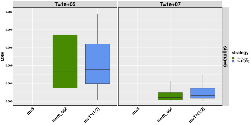
Figure S1: Zoom of boxplots of Figure 1 .

Figure 1 shows that the estimations obtained with Algorithm 2 are more accurate as $T$ gets large because both bias and variance are efficiently reduced. Boxplots highlight that the strategies $m=5$ and $m=T^{1/2}$ suffer respectively from bias and variance. Notice that in the case of the linear model under study, $\mathbb{E}(\text{Var}(f(X_{1},X_{2},Z)\mid(X_{1},X_{2})))=2\sigma^{2}$; so the bias depends on $\sigma$. This explains why in the case $\sigma=5$ (Figure 1), even for large value of $T$, estimations resulting of the choice $m=5$ seem not to decrease but are rather concentrated around about $0.18$ which is very large compared to what is obtained in the two other strategies. Focusing on strategies $m=m_{opt}$ and $m=T^{1/2}$, a zoom of the plot of Figure 1 for the case $\sigma=5$, given in Figure S1 in Appendix A, enables to compare them and then to confirm that the strategy implemented in Algorithm 2 provide more accurate estimations as $T$ increases.

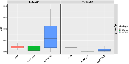
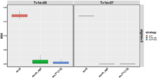
Figure 1: Boxplots of MSE estimates for the linear model for different values of $T$ and $\sigma$. Three strategies of choice of $m$ are compared: $m=5$ (in red), $m=m_{opt}$ given by the trade-off strategy of Algorithm 2 (in green) and $m=T^{1/2}$ (in blue).

A stochastic Ishigami function

Let $f^{\prime}(X_{1},X_{2},X_{3},Z)=\sin X_{1}+a\sin^{2}X_{2}+bX_{3}^{4}\sin X_{1}Z^{2}$ such that with $a,b>0$, $X_{1},X_{2},X_{3}$ and $Z$ are independent with $X_{1},X_{2},X_{3}$ distributed under $\mathcal{U}\left([-\pi,\pi]\right)$ and $Z\sim\mathcal{N}\left(0,1\right)$. The model $f^{\prime}$ is a modified version of benchmark function known as the Ishigami function in SA. For this model, first-order Sobol’ indices of inputs $X_{1},X_{2},$ and $X_{3}$ for the QoI $\mathbb{E}(f^{\prime}(X_{1},X_{2},X_{3},Z)\mid X_{1},X_{2},X3)$ are respectively given by $S_{1}=\frac{1}{2}\frac{\left(1+\frac{b\pi^{4}}{5}\right)^{2}}{\frac{a^{2}}{8}+\frac{b\pi^{4}}{5}+\frac{b^{2}\pi^{8}}{18}+\frac{1}{2}}$, $S_{2}=\frac{\frac{a^{2}}{8}}{\frac{a^{2}}{8}+\frac{b\pi^{4}}{5}+\frac{b^{2}\pi^{8}}{18}+\frac{1}{2}}$ and $S_{3}=0$. Parameters $a$ and $b$ are chosen with respect to Sobol’ and Levitan (1999): $a=7$, $b=0.05$ and Marrel et al. (2009): $a=7$, $b=0.1$.

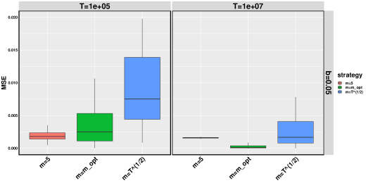
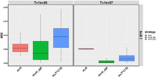
Figure 2: Boxplots of MSE estimates for the stochastic version of Ishigami function for different values of $T$ and $b$. Three strategies of choice of $m$ are compared: $m=5$ (in red), $m=m_{opt}$ given by the trade-off strategy of Algorithm 2 (in green) and $m=T^{1/2}$ (in blue).

Figure 2 also reveals that estimations obtained by using Algorithm 2 are more accurate for large $T$. Besides, remark that the term $bX_{3}^{4}\sin X_{1}$ that multiplies the intrinsic noise term $Z^{2}$ includes $b$ so that $|bX_{3}^{4}\sin X_{1}|\leq b\pi^{4}$. Then, $b$ allows to control the magnitude of the intrinsic noise term of the model. This explains why estimations in the case $b=0.1$ present much more variability compared to the case $b=0.05$. Nonetheless, in both cases the strategy implemented in Algorithm 2 has better results.

Overall, Figures 1 and 2 lead to the same conclusion: the strategy of Algorithm 2 provides better estimations and its MSE estimates decrease faster and are generally smaller compared to those of the two other estimators. In the particular case of $m=5$, it is noticeable that errors do not decrease when $T$ gets larger but rather they are quite constant. This is explained by the fact that the bias is constant since $m$ is constant. This illustrates the importance of varying the number of repetition when the total computational budget grows. Regarding the case $m=T^{1/2}$, it turns out that MSEs are not minimal compared to the case $m=m_{opt}$ due the variance part of those errors. Indeed, with $m=T^{1/2}$, the variance part of the BVT converges to $0$ at rate $T^{1/2}$ while the squared-bias part converges at rate $T$. Then, the global convergence rate of the BVT is $T^{1/2}$ that is slower than the rate $T^{2/3}$ of estimators built by Algorithm 2. These two cases clearly illustrate the bias-variance trade-off problem in Sobol’ index estimation for stochastic models and they allow to show that the strategy proposed in this paper performs well.

6 Conclusion

This paper focuses on variance-based SA of stochastic models relying on the approach that consists in performing SA on some deterministic QoIs. Specifically, it deals with QoIs under the form of conditional expectations with respect to the uncertain parameters of some transformation of the original stochastic model output. For such deterministic quantities, estimation of Sobol’ indices through Monte-Carlo methods (pick-freeze procedure) requires not only to sample the input space but also to estimate conditional expectations by making repetitions. Therefore, the resulting estimators depend on both the number of explorations $n$ and the number of repetitions $m$. This study pointed out that the MSE of such estimators can be bounded by tractable quantities that depend on both $n$ and $m$. This had two implications. First, the bounds enable to ensure that the MSE converges to zero when both $n,m\rightarrow+\infty$. Straightforwardly, this establishes that the estimators of Sobol’ indices converge in quadratic mean. Secondly, A strategy can be developed for controlling the bias-variance trade-off that arises when the product $nm$ is fixed. Indeed, the bias and the variance decrease respectively when $m\rightarrow+\infty$ and $n\rightarrow+\infty$. Under the constraint $nm=T$ and $T\to+\infty$, the numbers $m$ and $n$ should be chosen such that both the variance and the bias vanish at the fastest rate possible. This problem is discussed and this study showed that taking $m$ of order $T^{1/3}$ and $n$ of order $T^{2/3}$ guarantees that quantity BVT representing the bias-variance tradeoff in the MSE converges at rate at least $T^{2/3}$. Furthermore, the minimization of some upper bounds of the MSE under the constraint $nm=T$ provides a choice of $m$ and $n$ that adapts to the intrinsic randomness of the stochastic model. This strategy is implemented through two algorithms dedicated to Sobol’ index estimation based on the pick-freeze procedure. The comparison of this strategy to two others was carried out using two toy stochastic models. It turned out that the strategy proposed in this paper performs well.

For further works, it could be interesting to couple the iterative estimation approach of Gilquin et al. (2021) to the algorithms implemented in this study in order to build an adaptive version which could perform estimation with respect to a given precision. Furthermore, it would be interesting to compare the optimal BVT convergence rate of sensitivity index estimators based on basic Monte Carlo sampling with the rates one could get with other approaches, such as multilevel Monte Carlo methods (Mycek and De Lozzo (2019); Giles and Haji-Ali (2019)). Finally, although a convergence rate for the BVT has been found, that of the whole MSE remains an open problem.

Acknowledgment

We thank Clémentine Prieur for reading the first version of this paper and for the relevant remarks and references she suggested.

A Boxplot

B Proof of Theorem 1

Using convexity inequality, for all $h\in(0,1)$ and $m\geq 1$, it holds:

$$\mathbb{E}\left(g\left(\widehat{\theta}\right)-g\left(\theta\right)\right)^{2}\leq 3\mathbb{E}\left(g\left(\widehat{\theta}\right)-g\left(\widehat{\theta}+h\mathbf{u}\right)\right)^{2}+3\mathbb{E}\left(g\left(\widehat{\theta}+h\mathbf{u}\right)-g\left(\mu_{m}+h\mathbf{u}\right)\right)^{2}+$$

$$3\left(g\left(\mu_{m}+h\mathbf{u}\right)-g\left(\theta\right)\right)^{2}$$

Applying a Taylor-Lagrange expansion to $g$ at points $\widehat{\theta}+h\mathbf{u}$ and $\mu_{m}+h\mathbf{u}$ yields:

$$\mathbb{E}\left(g\left(\widehat{\theta}+h\mathbf{u}\right)-g\left(\mu_{m}+h\mathbf{u}\right)\right)^{2}$$

$$=\mathbb{E}\left(\nabla g\left(\mu_{m}+h\mathbf{u}\right)^{\top}\left(\widehat{\theta}-\mu_{m}\right)+\frac{1}{2}\left(\widehat{\theta}-\mu_{m}\right)^{\top}\nabla^{2}g\left(\lambda\widehat{\theta}+(1-\lambda)\mu_{m}+h\mathbf{u}\right)\left(\widehat{\theta}-\mu_{m}\right)\right)^{2}$$

$$\leq\mathbb{E}\left(\nabla g\left(\mu_{m}+h\mathbf{u}\right)^{\top}\left(\widehat{\theta}-\mu_{m}\right)\right)^{2}$$

$$\quad+\frac{1}{4}\mathbb{E}\left(\left(\widehat{\theta}-\mu_{m}\right)^{\top}\nabla^{2}g\left(\lambda\widehat{\theta}+(1-\lambda)\mu_{m}+h\mathbf{u}\right)\left(\widehat{\theta}-\mu_{m}\right)\right)^{2}$$

$$\quad+\sqrt{\mathbb{E}\left(\nabla g\left(\mu_{m}+h\mathbf{u}\right)^{\top}\left(\widehat{\theta}-\mu_{m}\right)\right)^{2}}\sqrt{\mathbb{E}\left(\left(\widehat{\theta}-\mu_{m}\right)^{\top}\nabla^{2}g\left(\lambda\widehat{\theta}+(1-\lambda)\mu_{m}+h\mathbf{u}\right)\left(\widehat{\theta}-\mu_{m}\right)\right)^{2}}$$

for some $\lambda\in(0,1)$. Thus:

$$\frac{\mathbb{E}\left(g\left(\widehat{\theta}+h\mathbf{u}\right)-g\left(\mu_{m}+h\mathbf{u}\right)\right)^{2}}{\mathbb{E}\left(\nabla g\left(\mu_{m}+h\mathbf{u}\right)^{\top}\left(\widehat{\theta}-\mu_{m}\right)\right)^{2}}$$

$$\leq\quad 1+\frac{1}{4}\frac{\mathbb{E}\left(\left(\widehat{\theta}-\mu_{m}\right)^{\top}\nabla^{2}g\left(\lambda\widehat{\theta}+(1-\lambda)\mu_{m}+h\mathbf{u}\right)\left(\widehat{\theta}-\mu_{m}\right)\right)^{2}}{\mathbb{E}\left(\nabla g\left(\mu_{m}+h\mathbf{u}\right)^{\top}\left(\widehat{\theta}-\mu_{m}\right)\right)^{2}}$$

$$\quad+\sqrt{\frac{\mathbb{E}\left(\left(\widehat{\theta}-\mu_{m}\right)^{\top}\nabla^{2}g\left(\lambda\widehat{\theta}+(1-\lambda)\mu_{m}+h\mathbf{u}\right)\left(\widehat{\theta}-\mu_{m}\right)\right)^{2}}{\mathbb{E}\left(\nabla g\left(\mu_{m}+h\mathbf{u}\right)^{\top}\left(\widehat{\theta}-\mu_{m}\right)\right)^{2}}}.$$

Let $\phi:x\mapsto x/4+\sqrt{x}$ and

$$p_{n,m}(h):=\phi\left(\sup_{\lambda\in[0,1]}\frac{\mathbb{E}\left(\left(\widehat{\theta}-\mu_{m}\right)^{\top}\nabla^{2}g\left(\lambda\widehat{\theta}+(1-\lambda)\mu_{m}+h\mathbf{u}\right)\left(\widehat{\theta}-\mu_{m}\right)\right)^{2}}{\mathbb{E}\left(\nabla g\left(\mu_{m}+h\mathbf{u}\right)^{\top}\left(\widehat{\theta}-\mu_{m}\right)\right)^{2}}\right).$$ (16)

then the ratio $\mathbb{E}\left(g\left(\widehat{\theta}+h\mathbf{u}\right)-g\left(\mu_{m}+h\mathbf{u}\right)\right)^{2}/\mathbb{E}\left(\nabla g\left(\mu_{m}+h\mathbf{u}\right)^{\top}\left(\widehat{\theta}-\mu_{m}\right)\right)^{2}$ is bounded by $1+p_{n,m}(h)$. Therefore:

$$\mathbb{E}\left(g\left(\widehat{\theta}+h\mathbf{u}\right)-g\left(\mu_{m}+h\mathbf{u}\right)\right)^{2} =\frac{\mathbb{E}\left(g\left(\widehat{\theta}+h\mathbf{u}\right)-g\left(\mu_{m}+h\mathbf{u}\right)\right)^{2}}{\mathbb{E}\left(\nabla g\left(\mu_{m}+h\mathbf{u}\right)^{\top}\left(\widehat{\theta}-\mu_{m}\right)\right)^{2}}\times\mathbb{E}\left(\nabla g\left(\mu_{m}+h\mathbf{u}\right)^{\top}\left(\widehat{\theta}-\mu_{m}\right)\right)^{2}$$

$$\leq(1+p_{n,m}(h))V_{n,m}(h).$$

Now, let us show that $p_{n,m}(h)\to 0$ as $n,m\to\infty$. For this purpose, it is sufficient to have that $\sup_{\lambda\in[0,1]}\tfrac{\mathbb{E}\left(\left(\widehat{\theta}-\mu_{m}\right)^{\top}\nabla^{2}g\left(\lambda\widehat{\theta}+(1-\lambda)\mu_{m}+h\mathbf{u}\right)\left(\widehat{\theta}-\mu_{m}\right)\right)^{2}}{\mathbb{E}\left(\nabla g\left(\mu_{m}+h\mathbf{u}\right)^{\top}\left(\widehat{\theta}-\mu_{m}\right)\right)^{2}}=o(1)$ as $n,m\rightarrow+\infty$. A first use of Cauchy-Schwarz inequality yields that:

$$\left(\left(\widehat{\theta}-\mu_{m}\right)^{\top}\nabla^{2}g\left(\lambda\widehat{\theta}+(1-\lambda)\mu_{m}+h\mathbf{u}\right)\left(\widehat{\theta}-\mu_{m}\right)\right)^{2}\leq\|\nabla^{2}g\left(\lambda\widehat{\theta}+(1-\lambda)\mu_{m}+h\mathbf{u}\right)\|_{F}^{2}\times\|\widehat{\theta}-\mu_{m}\|^{4}.$$

By a second use of Cauchy-Schwarz inequality, the argument of $\phi$ in Equation (16) is bounded by

$$\sqrt{\sup_{\lambda\in[0,1]}\mathbb{E}\left(\|\nabla^{2}g\left(\lambda\widehat{\theta}+(1-\lambda)\mu_{m}+h\mathbf{u}\right)\|_{F}^{4}\right)}\times\frac{\sqrt{\mathbb{E}\left(\|\widehat{\theta}-\mu_{m}\|^{8}\right)}}{\mathbb{E}\left(\nabla g\left(\mu_{m}+h\mathbf{u}\right)^{\top}\left(\widehat{\theta}-\mu_{m}\right)\right)^{2}}.$$

As $n,m\rightarrow\infty$, the first term of the product above is bounded by a constant independent of $h$, uniformly in $\lambda$, by Assumption 3. The second term is given by:

$$\frac{\sqrt{\mathbb{E}\left(\|\widehat{\theta}-\mu_{m}\|^{8}\right)}}{\mathbb{E}\left(\nabla g\left(\mu_{m}+h\mathbf{u}\right)^{\top}\left(\widehat{\theta}-\mu_{m}\right)\right)^{2}} =\frac{\sqrt{\mathbb{E}\left(\|\widehat{\theta}-\mu_{m}\|^{8}\right)}}{\mathbb{E}\left(\nabla g\left(\mu_{m}\right)^{\top}\left(\widehat{\theta}-\mu_{m}\right)\right)^{2}}\times\frac{\mathbb{E}\left(\nabla g\left(\mu_{m}\right)^{\top}\left(\widehat{\theta}-\mu_{m}\right)\right)^{2}}{\mathbb{E}\left(\nabla g\left(\mu_{m}+h\mathbf{u}\right)^{\top}\left(\widehat{\theta}-\mu_{m}\right)\right)^{2}}$$

$$\leq\frac{\sqrt{\mathbb{E}\left(\|\widehat{\theta}-\mu_{m}\|^{8}\right)}}{\mathbb{E}\left(\nabla g\left(\mu_{m}\right)^{\top}\left(\widehat{\theta}-\mu_{m}\right)\right)^{2}}\times\sup_{h\in(0,1)}\frac{\mathbb{E}\left(\nabla g\left(\mu_{m}\right)^{\top}\left(\widehat{\theta}-\mu_{m}\right)\right)^{2}}{\mathbb{E}\left(\nabla g\left(\mu_{m}+h\mathbf{u}\right)^{\top}\left(\widehat{\theta}-\mu_{m}\right)\right)^{2}}.$$ (17)

The first term in the right-hand side in (17) is of order $o(1)$ by Assumption 2 and does not depend on $h$. Moreover, since $\nabla g$ is continuous, we have $\sup_{h\in(0,1)}\frac{\mathbb{E}\left(\nabla g\left(\mu_{m}\right)^{\top}\left(\widehat{\theta}-\mu_{m}\right)\right)^{2}}{\mathbb{E}\left(\nabla g\left(\mu_{m}+h\mathbf{u}\right)^{\top}\left(\widehat{\theta}-\mu_{m}\right)\right)^{2}}=O(1)$ as $n,m\to\infty$. Therefore, the quantity in (16) is of order $\phi(o(1))=o(1)$, and hence

$$\mathbb{E}\left(g\left(\widehat{\theta}\right)-g\left(\theta\right)\right)^{2}\leq 3\left(1+p_{n,m}(h)\right)\left(\Delta_{n,m}(h)+V_{n,m}(h)+B_{m}(h)^{2}\right),$$

where $\lim_{n,m\to+\infty}p_{n,m}(h)=0$.

Let us focus on $\Delta_{n,m}(h)=\mathbb{E}\left(g(\widehat{\theta})-g(\widehat{\theta}+h\mathbf{u})\right)^{2}$. For this purpose, let $h\in(0,1)$. Using convexity inequality, the Taylor-Lagrange expansion provides that:

$$g(\widehat{\theta})-g(\widehat{\theta}+h\mathbf{u}) =h\nabla g(\widehat{\theta}+h\mathbf{u})^{\top}\mathbf{u}+\frac{1}{2}h^{2}\mathbf{u}^{\top}\nabla^{2}g(\widehat{\theta}+h\lambda\mathbf{u})\mathbf{u},$$

$$\mathbb{E}\left(g(\widehat{\theta})-g(\widehat{\theta}+h\mathbf{u})\right)^{2} \leq 2h^{2}\left(\mathbb{E}\left(\nabla g(\widehat{\theta}+h\mathbf{u})^{\top}\mathbf{u}\right)^{2}+\frac{h^{2}}{4}\mathbb{E}\left(\mathbf{u}^{\top}\nabla^{2}g(\widehat{\theta}+h\lambda\mathbf{u})\mathbf{u}\right)^{2}\right),$$

for some $\lambda\in(0,1)$. It appears that:

$$\mathbb{E}\left(\mathbf{u}^{\top}\nabla^{2}g(\widehat{\theta}+h\lambda\mathbf{u})\mathbf{u}\right)^{2}\leq\|\mathbf{u}\|^{4}\mathbb{E}\left(\|\nabla^{2}g(\widehat{\theta}+h\lambda\mathbf{u})\|_{F}^{2}\right).$$

Since $h\lambda\in(0,1)$, the right-hand side is bounded by a constant independent of $h$ and $\lambda$, as $n,m\to\infty$ (by Assumption 3). Regarding $\mathbb{E}\left(\nabla g(\widehat{\theta}+h\mathbf{u})^{\top}\mathbf{u}\right)^{2}$, an additional Taylor-Lagrange expansion of $\nabla g(\widehat{\theta}+h\mathbf{u})^{\top}\mathbf{u}$ yields:

$$\nabla g(\widehat{\theta}+h\mathbf{u})^{\top}\mathbf{u}=\nabla g(\mu_{m}+h\mathbf{u})^{\top}\mathbf{u}+\left(\widehat{\theta}-\mu_{m}\right)^{\top}\nabla^{2}g(\lambda\widehat{\theta}+(1-\lambda)\mu_{m}+h\mathbf{u})\mathbf{u}\\ \mathbb{E}\left(\nabla g(\widehat{\theta}+h\mathbf{u})^{\top}\mathbf{u}\right)^{2}\leq\left(\nabla g(\mu_{m}+h\mathbf{u})^{\top}\mathbf{u}\right)^{2}+\|\mathbf{u}\|^{2}\sqrt{\mathbb{E}\left(\|\widehat{\theta}-\mu_{m}\|^{4}\right)}\times\\ \sqrt{\sup_{\lambda\in[0,1]}\mathbb{E}\left(\|\nabla^{2}g(\lambda\widehat{\theta}+(1-\lambda)\mu_{m}+h\mathbf{u})\|_{F}^{4}\right)}$$

Then:

$$\mathbb{E}\left(g(\widehat{\theta})-g(\widehat{\theta}+h\mathbf{u})\right)^{2}\leq\tilde{p}_{n,m}(h)h^{2},$$

where:

$$\tilde{p}_{n,m}(h)=2\left(\sqrt{\sup_{\lambda\in[0,1]}\mathbb{E}\left(\|\nabla^{2}g(\lambda\widehat{\theta}+(1-\lambda)\mu_{m}+h\mathbf{u})\|_{F}^{4}\right)}+\left(\nabla g(\mu_{m}+h\mathbf{u})^{\top}\mathbf{u}\right)^{2}+\sqrt{\mathbb{E}\left(\|\widehat{\theta}-\mu_{m}\|^{4}\right)}\right.\times$$

$$\left.\sqrt{\sup_{\lambda\in[0,1]}\mathbb{E}\left(\|\nabla^{2}g(\lambda\widehat{\theta}+(1-\lambda)\mu_{m}+h\mathbf{u})\|_{F}^{4}\right)}\right).$$

Note that:

$$\limsup_{n,m\to\infty}\tilde{p}_{n,m}(h)\leq 2\left(\sqrt{C}+\sup_{h\in(0,1)}\|\nabla g(\theta+h\mathbf{u})\|^{2}\right)=:\tilde{C}<+\infty.$$

C Proof of Theorem 2

To prove Theorem 2, the following result is required.

Lemma C.1.

Let $\mathbf{X}^{(1)},\cdots,\mathbf{X}^{(n)}$ be $n$ i.i.d. copies of $\mathbf{X}$ and $Z^{(1,1)},\cdots,Z^{(n,m)}$ be $n\times m$ i.i.d. copies of $Z$ such that $(\mathbf{X}^{(1)},\cdots,\mathbf{X}^{(n)})$ and $(Z^{(1,1)},\cdots,Z^{(n,m)})$ are independent. Then, for all $q\in\mathbb{N}$: $m^{-q}\mathbb{E}\left(\sum_{k=1}^{m}\varphi(\mathbf{X}^{(1)},Z^{(1,k)})\right)^{q}$ is polynomial in $m^{-1}$ of degree $q-1$ with constant $\mathbb{E}\left(\mathbb{E}\left[\varphi(\mathbf{X},Z)\mid\mathbf{X}\right]\right)^{q}$.

First, let us bound the numerator of the ratio in Assumption 2; we have

$$\mathbb{E}\left(\|\widehat{\theta}-\mu_{m}\|^{8}\right)\leq 27\sum_{j=1}^{3}\mathbb{E}\left(\|\widehat{\theta}_{j}-\mu_{mj}\|^{8}\right),$$

where $\widehat{\theta}_{j}$ and $\mu_{mj}$ denote the $j$th component of $\widehat{\theta}$ and $\mu_{m}$, respectively. By Marcinkiewicz and Zygmund (1937) and Jensen inequalities, we have for every $j$ that

$$\mathbb{E}\left(\|\widehat{\theta}_{j}-\mu_{mj}\|^{8}\right)\leq\frac{B_{8}}{n^{4}}\mathbb{E}\left(\left|\widehat{\theta}_{mj}^{(1)}-\mu_{mj}\right|^{8}\right),$$

where here $B_{8}$ is a universal constant.

The case $j=2$ is the simplest. Notice that $\mu_{m2}$ does not depend on $m$, then the expansion of $\mathbb{E}(|\widehat{Q}_{m}(\mathbf{X}^{(1)})-\mu_{m2}|^{8})$ through Newton formula yields terms of the form $\mu_{m2}^{k}\mathbb{E}(\widehat{Q}_{m}^{8-k}),k=0,\dots,8$. Using Lemma  C.1 provides that those terms are polynomial in $m^{-1}$.

Let us deal with the case $j=1$. Expanding the power $8$ through Newton’s formula and bounding its terms yields

$$\mathbb{E}\left(\left|\widehat{Q}_{m}(\mathbf{X}^{(1)})^{2}-\mu_{m1}\right|^{8}\right)\leq(\mu_{m1}^{8}\vee 1)\binom{8}{4}\left(\mathbb{E}\left(\widehat{Q}_{m}(\mathbf{X}^{(1)})^{16}\right)+1\right).$$ (18)

Denoting $\varphi(\mathbf{X}^{(1)},Z^{(1,k)})=Y^{(1,k)}$, we have

$$\mathbb{E}\left(\left|\widehat{Q}_{m}(\mathbf{X}^{(1)})\right|^{16}\right) =\mathbb{E}\left(\left|\frac{1}{m}\sum_{k=1}^{m}Y^{(1,k)}\right|^{16}\right)$$

$$=\frac{1}{m^{16}}\sum_{k_{1},\dots,k_{16}=1}^{m}\mathbb{E}\left(Y^{(1,k_{1})}\cdots Y^{(1,k_{16})}\right).$$

The expectation in the right-hand side is symmetric in $k_{1},\dots,k_{16}$, and hence, from Lemma C.1, the sum is a polynomial in $m$ of degree $16$. Therefore, the right-hand side in (18) is bounded uniformly in $m$.

Let us deal with the case $j=3$. Proceeding as in (18), we have

$$\mathbb{E}\left(\left|\widehat{Q}_{m}(\mathbf{X}^{(1)})\widetilde{Q}_{m}(\widetilde{\mathbf{X}}^{(1)}_{\sim u},\mathbf{X}^{(1)}_{u})-\mu_{m3}\right|^{8}\right)$$

$$\leq(\mu_{m3}^{8}\vee 1)\binom{8}{4}\left(\mathbb{E}\left(\left|\widehat{Q}_{m}(\mathbf{X}^{(1)})\widetilde{Q}_{m}(\widetilde{\mathbf{X}}^{(1)}_{\sim u},\mathbf{X}^{(1)}_{u})\right|^{8}\right)+1\right)$$

$$\leq(\mu_{m3}^{8}\vee 1)\binom{8}{4}\left(\mathbb{E}\left(\frac{1}{2}\widehat{Q}_{m}(\mathbf{X}^{(1)})^{16}+\frac{1}{2}\widetilde{Q}_{m}(\widetilde{\mathbf{X}}^{(1)}_{\sim u},\mathbf{X}^{(1)}_{u})^{16}\right)+1\right),$$

and this is also bounded uniformly in $m$. (Again by Lemma C.1.)

We now deal with the root of the denominator of the ratio in Assumption 2. We have

$$\mathbb{E}\left(\nabla g\left(\mu_{m}\right)^{T}\left(\widehat{\theta}-\mu_{m}\right)\right)^{2}$$

$$=\sum_{j_{1},j_{2}=1}^{3}\nabla g(\mu_{m})_{j_{1}}\nabla g(\mu_{m})_{j_{2}}\mathbb{E}(\widehat{\theta}-\mu_{m})_{j_{1}}(\widehat{\theta}-\mu_{m})_{j_{2}}$$

$$=\frac{1}{n}\sum_{j_{1},j_{2}=1}^{3}\nabla g(\mu_{m})_{j_{1}}\nabla g(\mu_{m})_{j_{2}}\left(\mathbb{E}\widehat{\theta}^{(1)}_{mj_{1}}\widehat{\theta}^{(1)}_{mj_{2}}-\mu_{mj_{1}}\mu_{mj_{2}}\right).$$ (19)

The infimum of the sum in (19) is reached for some $m$ and greater than zero. Therefore, the numerator in Assumption 2 is less than $1/n^{4}$ times a constant not depending on $m$ or $n$ and the denominator is equal to $1/n^{2}$ times a quantity greater than zero. Therefore, the supremum over $m$ of the ratio in Assumption 2 is of order $O(n^{-2})$. The proof is complete.

Proof of Lemma C.1

It holds that:

$$\mathbb{E}\left(\frac{1}{m}\sum_{k=1}^{m}\varphi(\mathbf{X}^{(1)},Z^{(1,k)})\right)^{q} =\frac{1}{m^{q}}\mathbb{E}\left(\sum_{k_{1}=1}^{m}\cdots\sum_{k_{q}=1}^{m}\varphi(\mathbf{X}^{(1)},Z^{(1,k_{1})})\cdots\varphi(\mathbf{X}^{(1)},Z^{(1,k_{q})})\right)$$

$$=\frac{1}{m^{q}}\sum_{k_{1}=1}^{m}\cdots\sum_{k_{q}=1}^{m}\mathbb{E}\left(\varphi(\mathbf{X}^{(1)},Z^{(1,k_{1})})\cdots\varphi(\mathbf{X}^{(1)},Z^{(1,k_{q})})\right).$$

Denote by $\lambda:\{1,\dots,m\}^{q}\to\mathbb{N}$ the map which with each $\mathbf{k}:=(k_{1},\dots,k_{q})$ associates the number of distinct indices among $k_{1},\dots,k_{q}$. If $1\leq l\leq q$ then denote by $\rho_{l}:\lambda^{-1}(l)\to\{1,\dots,q\}^{l}$ the map which with each $\mathbf{k}\in\lambda^{-1}(l)$ associates $(r_{1},\dots,r_{l})$, where $r_{i}=|\{j:k_{j}=k_{j_{i}}\}|$ for every $i=1,\dots,l$ and $k_{j_{1}},\dots,k_{j_{l}}$ are the distinct indices found among $k_{1},\dots,k_{q}$. Obviously, $r_{1}+\cdots+r_{l}=q$. We have

$$\sum_{k_{1}=1}^{m}\cdots\sum_{k_{q}=1}^{m}\mathbb{E}\left(\varphi(\mathbf{X}^{(1)},Z^{(1,k_{1})})\cdots\varphi(\mathbf{X}^{(1)},Z^{(1,k_{q})})\right)$$

$$=\sum_{k_{1}=1}^{m}\cdots\sum_{k_{q}=1}^{m}f(\mathbf{k})$$

$$=\sum_{l=1}^{q}\left(\sum_{(r_{1},\dots,r_{l})\in\{1,\dots,q\}^{l}:r_{1}+\cdots+r_{l}=q}\left(\sum_{\mathbf{k}\in\lambda^{-1}(l):\rho_{l}(\mathbf{k})=(r_{1},\dots,r_{l})}f(\mathbf{k})\right)\right).$$ (20)

Now, since

$$\mathbb{E}\left(\varphi(\mathbf{X}^{(1)},Z^{(1,k_{1})})\cdots\varphi(\mathbf{X}^{(1)},Z^{(1,k_{q})})\right)$$

$$=\mathbb{E}\left(\varphi(\mathbf{X}^{(1)},Z^{(1,k_{j_{1}})})^{r_{1}}\cdots\varphi(\mathbf{X}^{(1)},Z^{(1,k_{j_{l}})})^{r_{l}}\right)$$

$$=\mathbb{E}\left(\prod_{s=1}^{l}\mathbb{E}\left[\varphi(\mathbf{X}^{(1)},Z^{(1,k_{j_{s}})})^{r_{s}}\mid\mathbf{X}^{(1)}\right]\right)$$

is symmetric in $r_{1},\dots,r_{l}$, it holds that

$$\sum_{(r_{1},\dots,r_{l})\in\{1,\dots,q\}^{l}:r_{1}+\cdots+r_{l}=q}\left(\sum_{\mathbf{k}\in\lambda^{-1}(l):\rho_{l}(\mathbf{k})=(r_{1},\dots,r_{l})}f(\mathbf{k})\right)$$

$$=c(l,(r_{1},\dots,r_{l}),m)\mathbb{E}\left(\prod_{s=1}^{l}\mathbb{E}\left[\varphi(\mathbf{X}^{(1)},Z^{(1,k_{j_{s}})})^{r_{s}}\mid\mathbf{X}^{(1)}\right]\right)$$

where

$$c(l,(r_{1},\dots,r_{l}),m)=\binom{q}{r_{1}}\binom{q-r_{1}}{r_{2}}\cdots\binom{q-r_{1}-\cdots-r_{l-1}}{r_{l}}\\ m(m-1)\cdots(m-l+1).$$ (21)

Notice that the expression in the right-hand side of (21) is invariant by permutation of $r_{1},\dots,r_{l}$. Therefore, the sum (C) is a polynomial in $m$ of degree $q$ with constant zero and hence $\mathbb{E}\left(\frac{1}{m}\sum_{k=1}^{m}\varphi(\mathbf{X}^{(1)},Z^{(1,k})\right)^{q}$ is a polynomial in $\frac{1}{m}$ of degree $q-1$ with constant $\lim_{m\rightarrow+\infty}\mathbb{E}\left(\frac{1}{m}\sum_{k=1}^{m}\varphi(\mathbf{X}^{(1)},Z^{(1,k})\right)^{q}=\mathbb{E}\left(\mathbb{E}\left[\varphi(\mathbf{X},Z)\mid\mathbf{X}\right]\right)^{q}$.

D Proof of Theorem 3

The following lemma will be needed:

Lemma D.1.

For all $\alpha>0$ and all $h\in(0,1)$,

$$\lim_{n,m\to+\infty}\mathbb{E}\left[\frac{1}{\left(h+\widehat{\theta}_{1}-\widehat{\theta}_{2}^{2}\right)^{\alpha}}\right]=\frac{1}{\left(h+\text{Var}\left(Q(\mathbf{X})\right)\right)^{\alpha}}\leq\text{Var}\left(Q(\mathbf{X})\right)^{-\alpha}.$$ (22)

Note that the function $g$ is infinitely differentiable over its domain $\mathcal{D}$ and then its gradient is given by:

$$\nabla g\left(\theta_{1},\theta_{2},\theta_{3}\right)=\left(-\frac{\theta_{3}-\theta_{2}^{2}}{(\theta_{1}-\theta_{2}^{2})^{2}}\,\frac{2\theta_{2}(\theta_{3}-\theta_{1})}{(\theta_{1}-\theta_{2}^{2})^{2}},\frac{1}{\theta_{1}-\theta_{2}^{2}}\right)^{\top}.$$

Furthermore, the hessian matrix of $g$ yields:

$$\nabla^{2}g(\theta_{1},\theta_{2},\theta_{3})=\left(\begin{array}[]{ccc}\frac{2(\theta_{3}-\theta_{2}^{2})}{(\theta_{1}-\theta_{2}^{2})^{3}}&\frac{2\theta_{2}(\theta_{1}-2\theta_{3}+\theta_{2}^{2})}{(\theta_{1}-\theta_{2}^{2})^{3}}&\frac{-1}{(\theta_{1}-\theta_{2}^{2})^{2}}\\ \frac{2\theta_{2}(\theta_{1}-2\theta_{3}+\theta_{2}^{2})}{(\theta_{1}-\theta_{2}^{2})^{3}}&\frac{2(\theta_{3}-\theta_{1})(\theta_{1}+3\theta_{2}^{2})}{(\theta_{1}-\theta_{2}^{2})^{3}}&\frac{2\theta_{2}}{(\theta_{1}-\theta_{2}^{2})^{2}}\\ \frac{-1}{(\theta_{1}-\theta_{2}^{2})^{2}}&\frac{2\theta_{2}}{(\theta_{1}-\theta_{2}^{2})^{2}}&0\end{array}\right).$$

For any $(\theta_{1},\theta_{2},\theta_{3})\in\mathcal{D}$, the matrix $\nabla^{2}g(\theta_{1},\theta_{2},\theta_{3})$ is under the form $\nabla^{2}g(\theta_{1},\theta_{2},\theta_{3})=B(\theta_{1},\theta_{2},\theta_{3})/(\theta_{1}-\theta_{2}^{2})^{3}$ where $B(\theta_{1},\theta_{2},\theta_{3})$ is the matrix:

$$B(\theta_{1},\theta_{2},\theta_{3})=\left(\begin{array}[]{ccc}2(\theta_{3}-\theta_{2}^{2})&2\theta_{2}(\theta_{1}-2\theta_{3}+\theta_{2}^{2})&-(\theta_{1}-\theta_{2}^{2})\\ 2\theta_{2}(\theta_{1}-2\theta_{3}+\theta_{2}^{2})&2(\theta_{3}-\theta_{1})(\theta_{1}+3\theta_{2}^{2})&2\theta_{2}(\theta_{1}-\theta_{2}^{2})\\ -(\theta_{1}-\theta_{2}^{2})&2\theta_{2}(\theta_{1}-\theta_{2}^{2})&0\end{array}\right).$$

Notice that $B(\theta_{1},\theta_{2},\theta_{3})$ includes only multivariate polynomials of variables $\theta_{1},\theta_{2}$ and $\theta_{3}$.

Let us check Assumption 3. Let $\lambda\in[0,1]$ and $h\in(0,1)$. We have

$$\nabla^{2}g\left(\lambda\widehat{\theta}+(1-\lambda)\mu_{m}+h\mathbf{u}\right) =\frac{B\left(\lambda\widehat{\theta}+(1-\lambda)\mu_{m}+h\mathbf{u}\right)}{\left(h+\lambda\widehat{\theta}_{1}+(1-\lambda)\mu_{m1}-\left(\lambda\widehat{\theta}_{2}+(1-\lambda)\mu_{m2}\right)^{2}\right)^{3}}.$$

Thus:

$$\mathbb{E}\left(\|\nabla^{2}g\left(\lambda\widehat{\theta}+(1-\lambda)\mu_{m}+h\mathbf{u}\right)\|^{4}_{F}\right)$$

$$=\mathbb{E}\left(\frac{\|B\left(\lambda\widehat{\theta}+(1-\lambda)\mu_{m}+h\mathbf{u}\right)\|^{4}_{F}}{\left(h+\lambda\widehat{\theta}_{1}+(1-\lambda)\mu_{m1}-\left(\lambda\widehat{\theta}_{2}+(1-\lambda)\mu_{m2}\right)^{2}\right)^{12}}\right)$$

$$\leq\sqrt{\mathbb{E}\left(\frac{1}{\left(h+\lambda\widehat{\theta}_{1}+(1-\lambda)\mu_{m1}-\left(\lambda\widehat{\theta}_{2}+(1-\lambda)\mu_{m2}\right)^{2}\right)^{24}}\right)}$$

$$\quad\times\sqrt{\mathbb{E}\left(\|B\left(\lambda\widehat{\theta}+(1-\lambda)\mu_{m}+h\mathbf{u}\right)\|^{8}_{F}\right)}$$

$$\leq\sqrt{\mathbb{E}\left(\frac{1}{\left(h+\lambda\left(\widehat{\theta}_{1}-\widehat{\theta}_{2}^{2}\right)+(1-\lambda)(\mu_{m1}-\mu_{m1}^{2})\right)^{24}}\right)}\qquad\text{ (by convexity inequality) }$$

$$\quad\times\sqrt{\mathbb{E}\left(\|B\left(\lambda\widehat{\theta}+(1-\lambda)\mu_{m}+h\mathbf{u}\right)\|^{8}_{F}\right)}$$

$$\leq\sqrt{\mathbb{E}\left(\frac{\lambda}{\left(h+\left(\widehat{\theta}_{1}-\widehat{\theta}_{2}^{2}\right)\right)^{24}}\right)+\frac{1-\lambda}{(h+\mu_{m1}-\mu_{m1}^{2})^{24}}}\qquad\text{ (by convexity inequality) }$$

$$\quad\times\sqrt{\mathbb{E}\left(\|B\left(\lambda\widehat{\theta}+(1-\lambda)\mu_{m}+h\mathbf{u}\right)\|^{8}_{F}\right)}$$

$$\leq\sqrt{\mathbb{E}\left(\frac{1}{\left(h+\left(\widehat{\theta}_{1}-\widehat{\theta}_{2}^{2}\right)\right)^{24}}\right)+\frac{1}{(h+\mu_{m1}-\mu_{m1}^{2})^{24}}}$$

$$\quad\times\sqrt{\sup_{\lambda\in[0,1]}\mathbb{E}\left(\|B\left(\lambda\widehat{\theta}+(1-\lambda)\mu_{m}+h\mathbf{u}\right)\|^{8}_{F}\right)}$$

$$\leq\sqrt{\mathbb{E}\left(\frac{1}{\left(h+\left(\widehat{\theta}_{1}-\widehat{\theta}_{2}^{2}\right)\right)^{24}}\right)+\sup_{h\in(0,1)}\frac{1}{(h+\mu_{m1}-\mu_{m1}^{2})^{24}}}$$

$$\quad\times\sqrt{\sup_{h\in(0,1)}\sup_{\lambda\in[0,1]}\mathbb{E}\left(\|B\left(\lambda\widehat{\theta}+(1-\lambda)\mu_{m}+h\mathbf{u}\right)\|^{8}_{F}\right)}.$$

One should remark that $\sup_{h\in(0,1)}\frac{1}{(h+\mu_{m1}-\mu_{m1}^{2})^{24}}\leq\frac{1}{(\text{Var}\left(\mathbb{E}\left[\varphi(\mathbf{X},Z)\mid\mathbf{X}\right]\right))^{24}}<+\infty$. Moreover, the matrix $B$ is composed with polynomials of three variables. Since $\mathbb{E}\left(Q(\mathbf{X})^{16}\right)<+\infty$ then by using Lemma C.1 and by continuity of polynomial functions, it yields that $\sup_{h\in(0,1)}\sup_{\lambda\in[0,1]}\mathbb{E}\left(\|B\left(\lambda\widehat{\theta}+(1-\lambda)\mu_{m}+h\mathbf{u}\right)\|^{8}_{F}\right)$ is bounded. Finally, by relying on Lemma D.1, $\mathbb{E}(h+\widehat{\theta}_{1}-\widehat{\theta}_{2}^{2})^{-24}$ is a bounded by $\frac{1}{(\text{Var}\left(\mathbb{E}\left[\varphi(\mathbf{X},Z)\mid\mathbf{X}\right]\right))^{24}}$ as $n,m\rightarrow+\infty$. Therefore, Assumption 3 is satisfied.

Proof of Lemma D.1

Let $h\in(0,1)$ be fixed. The function $\beta_{h}:x\mapsto 1/(h+x)^{\alpha}$ is continuously differentiable such that its first derivative is uniformly bounded on $\mathbb{R}_{+}$ by $1/h^{\alpha+1}$ then it is Lipschitz. Therefore:

$$\mathbb{E}\left(\beta_{h}(\widehat{\theta}_{1}-\widehat{\theta}_{2}^{2})-\beta_{h}(\theta_{1}-\theta_{2}^{2})\right)^{2} \leq\frac{1}{h^{2\alpha+2}}\mathbb{E}\left(\widehat{\theta}_{1}-\widehat{\theta}_{2}^{2}-\theta_{1}+\theta_{2}^{2}\right)^{2}$$

$$\leq\frac{2}{h^{2\alpha+2}}\left(\text{Var}(\widehat{\theta}_{1})+\text{Var}(\widehat{\theta}_{2}^{2})+\left(\mathbb{E}(\widehat{\theta}_{2}^{2})-\theta_{2}^{2}\right)^{2}\right),$$

using convexity inequality. Based on Marcinkiewicz-Zygmund inequality (see Theorem H.1) and Lemma C.1, it follows that

$$\lim_{n,m\to\infty}\left((\text{Var}(\widehat{\theta}_{1})+\text{Var}(\widehat{\theta}_{2}^{2})+\left(\mathbb{E}(\widehat{\theta}_{2}^{2})-\theta_{2}^{2}\right)^{2}\right)=0.$$

Straightforwardly:

$$\lim_{n,m\to\infty}\mathbb{E}\left(\frac{1}{(h+(\widehat{\theta}_{1}-\widehat{\theta}_{2}^{2})^{\alpha}}\right)=\frac{1}{(h+\theta_{1}-\theta_{2}^{2})^{\alpha}}\leq\frac{1}{\text{Var}(Q(\mathbf{X}))^{\alpha}}.$$

E Proof of Corollary 1

Relying on Theorem 1 , it holds that:

$$\limsup_{n,m\to\infty}\mathbb{E}\left(g(\widehat{\theta})-g(\theta)\right)^{2} \leq 3\limsup_{n,m\to\infty}\left(1+p_{n,m}(h)\right)\left(\Delta_{n,m}(h)+V_{n,m}(h)+B_{m}(h)^{2}\right)$$

$$\leq 3\left(\tilde{C}h^{2}+\left(g(\theta+h\mathbf{u})-g(\theta)\right)^{2}\right).$$

Notice that the MSE is independent of $h$. Moreover, $\tilde{C}$ is also independent of $h$. Thus, relying on the continuity of $g$ and taking the limit as $h\to 0$ yields that:

$$\limsup_{n,m\to\infty}\mathbb{E}\left(g(\widehat{\theta})-g(\theta)\right)^{2}=0.$$

Hence $\lim_{n,m\to\infty}\mathbb{E}\left(g(\widehat{\theta})-g(\theta)\right)^{2}=0.$

F Proof of Proposition 1

The problem of optimal rate comes down to find $\beta_{max}=\max\{\beta\geq 0\mid T^{\beta}\mathbb{E}(g(\widehat{\theta})-g(\theta))^{2}=O(1)\}$. Using $\mathbb{E}(g(\widehat{\theta})-g(\theta))^{2}=O(T^{\eta-1})+O(T^{-2\eta})$ yields $T^{\beta}\mathbb{E}(g(\widehat{\theta})-g(\theta))^{2}=O(T^{\beta+\eta-1})+O(T^{\beta-2\eta})$. Thus, to obtain condition $T^{\beta}\mathbb{E}(g(\widehat{\theta})-g(\theta))^{2}=O(1)$, it suffices that:

$$\begin{cases}\beta+\eta-1\leq 0\\ \beta-2\eta\leq 0\end{cases}$$ (23)

The maximal value of $\beta$ that satisfies the system (23) is $\beta_{max}=2/3$. This maximal value corresponds to to $\eta=1/3$. Therefore, $m$ and $n$ are respectively of order $T^{1/3}$ and $T^{2/3}$.

G Proof of Proposition 2

Choose $f$, $\varphi$ and a law for $\mathbf{X}$ such that $\varphi(\mathbf{X},Z)\in(a,b)$ almost surely, where $0<a<b$. Thus, there exists $C>0$ such that $\widehat{\theta}_{1}-\widehat{\theta}_{2}^{2}\leq\frac{1}{C}$. Hence:

$$\mathbb{E}\left(g(\widehat{\theta})-g(\theta)\right)^{2}\geq C\,\mathbb{E}\left(\widehat{\theta}_{3}-\widehat{\theta}_{2}^{2}-g(\theta)(\widehat{\theta}_{1}-\widehat{\theta}_{2}^{2}\right)^{2}$$ (24)

Let:

$$\begin{cases}\widehat{\varepsilon}_{1}=\widehat{\theta}_{1}-\theta_{1}\\ \widehat{\varepsilon}_{2}=\widehat{\theta}_{2}^{2}-\theta_{2}^{2}\\ \widehat{\varepsilon}_{3}=\widehat{\theta}_{3}-\theta_{3}\end{cases}$$

Using the definition of $g$, Equation (24) leads to:

$$\mathbb{E}\left(g(\widehat{\theta})-g(\theta)\right)^{2}\geq C\,\mathbb{E}\left(-g(\theta)\widehat{\varepsilon}_{1}-(1-g(\theta))\widehat{\varepsilon}_{2}+\widehat{\varepsilon}_{3}\right)^{2}.$$ (25)

Tedious but standard calculations show that

$$\mathbb{E}\left(\widehat{\varepsilon}_{1}\right)^{2} =\frac{P_{1}(\frac{1}{m})}{n}+\left(\frac{cste}{m}\right)^{2}$$

$$\mathbb{E}\left(\widehat{\varepsilon}_{2}\widehat{\varepsilon}_{1}\right) =\frac{P_{2}^{(1)}(\frac{1}{m})}{n^{2}}+\frac{P_{2}^{(2)}(\frac{1}{m})}{n}$$

$$\mathbb{E}\left(\widehat{\varepsilon}_{3}\widehat{\varepsilon}_{1}\right) =\frac{P_{3}(\frac{1}{m})}{n}$$

$$\mathbb{E}\left((1-g(\theta))\widehat{\varepsilon}_{2}-\widehat{\varepsilon}_{3}\right)^{2} =\frac{P_{4}^{(1)}(\frac{1}{m})}{n^{2}}+\frac{P_{4}^{(2)}(\frac{1}{m})}{n}$$

where $P_{i}^{(j)}(\tfrac{1}{m})$, $i=1,\dots,4$, $j=1,2$, are polynomials in $\tfrac{1}{m}$ of degree at most 3. Hence, letting $R(\tfrac{1}{m})$ be a polynomial in $\tfrac{1}{m}$ of degree at most 3, the MSE satisfies:

$$\mathbb{E}\left(g(\widehat{\theta})-g(\theta)\right)^{2}\geq\frac{R(\frac{1}{m})}{n}+\left(\frac{cste}{m}\right)^{2}+O(n^{-2}).$$

Since the lower bound has rate $T^{2/3}$ with $m=T^{1/3}$ and $n=T^{2/3}$, it follows that, under the constraint $nm=T$ and for $T\rightarrow\infty$, the rate of the MSE is at least $T^{2/3}$.

H The Marcinkiewicz-Zygmund inequality

Theorem H.1 (Marcinkiewicz and Zygmund (1937)).

Let $U_{1},\cdots,U_{n}$ be i.i.d. random variables such that $\mathbb{E}(U_{1})=0$ and $\mathbb{E}|U_{1}|^{q}<+\infty$, where $1\leq q<+\infty$. There exist $A_{q}$ and $B_{q}$ depending only on $q$ such that:

$$A_{q}\mathbb{E}\left(\left(\sum_{i=1}^{n}\left|U_{i}\right|^{2}\right)^{\frac{q}{2}}\right)\leq\mathbb{E}\left(\left|\sum_{i=1}^{n}U_{i}\right|^{q}\right)\leq B_{q}\mathbb{E}\left(\left(\sum_{i=1}^{n}\left|U_{i}\right|^{2}\right)^{\frac{q}{2}}\right)$$

Furthermore, there exists $C_{q}$ independent from $n$ such that:

$$\mathbb{E}\left(\left|\frac{1}{n}\sum_{i=1}^{n}U_{i}\right|^{q}\right)\leq\frac{C_{q}}{n^{\frac{q}{2}}}.$$ (26)

References

Binois et al. (2018)
Mickaël Binois, Robert B. Gramacy, and Mike Ludkovski.
Practical heteroscedastic gaussian process modeling for large
simulation experiments.
Journal of Computational and Graphical Statistics, 27(4):808–821, 2018.
doi: 10.1080/10618600.2018.1458625.
Binois et al. (2019)
Mickaël Binois, Jiangeng Huang, Robert B. Gramacy, and Mike Ludkovski.
Replication or exploration? sequential design for stochastic
simulation experiments.
Technometrics, 61(1):7–23, 2019.
doi: 10.1080/00401706.2018.1469433.
Castellan et al. (2020)
G. Castellan, A. Cousien, and V.C. Tran.
Non-parametric adaptive estimation of order 1 Sobol indices in
stochastic models, with an application to Epidemiology.
Electronic Journal of Statistics, 14(1):50
– 81, 2020.
doi: 10.1214/19-EJS1627.
Chen and Zhou (2014)
Xi Chen and Qiang Zhou.
Sequential experimental designs for stochastic kriging.
In Proceedings of the Winter Simulation Conference 2014, pages
3821–3832, 2014.
doi: 10.1109/WSC.2014.7020209.
Chen and Zhou (2017)
Xi Chen and Qiang Zhou.
Sequential design strategies for mean response surface metamodeling
via stochastic kriging with adaptive exploration and exploitation.
European Journal of Operational Research, 262(2):575–585, 2017.
ISSN 0377-2217.
doi: https://doi.org/10.1016/j.ejor.2017.03.042.
Courcoul et al. (2011)
A. Courcoul, H. Monod, M. Nielen, D. Klinkenberg, L. Hogerwerf, F. Beaudeau,
and E. Vergu.
Modelling the effect of heterogeneity of shedding on the within herd
coxiella burnetii spread and identification of key parameters by sensitivity
analysis.
Journal of Theoretical Biology, 284(1):130–141, 2011.
ISSN 0022-5193.
doi: https://doi.org/10.1016/j.jtbi.2011.06.017.
da Veiga (2021)
S. da Veiga.
Kernel-based anova decomposition and shapley effects – application
to global sensitivity analysis, 2021.
arXiv:2101.05487.
da Veiga and Gamboa (2013)
S. da Veiga and F Gamboa.
Efficient estimation of sensitivity indices.
Journal of Nonparametric Statistics, 25(3):573–595, 2013.
doi: 10.1080/10485252.2013.784762.
da Veiga et al. (2017)
S. da Veiga, J-M Loubes, and M. Solís.
Efficient estimation of conditional covariance matrices for dimension
reduction.
Communications in Statistics - Theory and Methods, 46(9):4403–4424, 2017.
doi: 10.1080/03610926.2015.1083109.
Étoré et al. (2020)
P. Étoré, C. Prieur, D. K. Pham, and L. Li.
Global Sensitivity Analysis for Models Described by
Stochastic Differential Equations.
Methodology and Computing in Applied Probability, 22(2):803–831, June 2020.
ISSN 1387-5841, 1573-7713.
doi: 10.1007/s11009-019-09732-6.
Fort et al. (2013)
J-C. Fort, T. Klein, A. Lagnoux, and B. Laurent.
Estimation of the sobol indices in a linear functional
multidimensional model.
Journal of Statistical Planning and Inference, 143(9):1590–1605, 2013.
ISSN 0378-3758.
doi: https://doi.org/10.1016/j.jspi.2013.04.007.
Fort et al. (2021)
J-C. Fort, T. Klein, and A. Lagnoux.
Global sensitivity analysis and wasserstein spaces.
SIAM/ASA Journal on Uncertainty Quantification, 9(2):880–921, 2021.
doi: 10.1137/20M1354957.
Gamboa et al. (2016)
F. Gamboa, A. Janon, T. Klein, A. Lagnoux, and C. Prieur.
Statistical inference for sobol pick-freeze monte carlo method.
Statistics, 50(4):881–902, 2016.
doi: 10.1080/02331888.2015.1105803.
Gamboa et al. (2021)
F. Gamboa, T. Klein, A. Lagnoux, and L. Moreno.
Sensitivity analysis in general metric spaces.
Reliability Engineering & System Safety, 212:107611, 2021.
Giles and Haji-Ali (2019)
M. B. Giles and A.-L. Haji-Ali.
Multilevel nested simulation for efficient risk estimation.
SIAM/ASA Journal on Uncertainty Quantification, 7(2):497–525, 2019.
Giles (2018)
Michael B. Giles.
MLMC for Nested Expectations, pages 425–442.
Springer International Publishing, Cham, 2018.
ISBN 978-3-319-72456-0.
doi: 10.1007/978-3-319-72456-0-20.
Gilquin et al. (2021)
L. Gilquin, C. Prieur, E. Arnaud, and H. Monod.
Iterative estimation of Sobol’ indices based on replicated
designs.
Computational and Applied Mathematics, 40(1):18, January 2021.
ISSN 1807-0302.
doi: 10.1007/s40314-020-01402-5.
Giorgi et al. (2017)
D. Giorgi, V. Lemaire, and G. Pagès.
Limit theorems for weighted and regular multilevel estimators.
Monte Carlo Methods and Applications, 23(1):43–70, 2017.
doi: doi:10.1515/mcma-2017-0102.
Giorgi et al. (2020)
D. Giorgi, V. Lemaire, and G. Pagès.
Weak Error for Nested Multilevel Monte Carlo.
Methodology and Computing in Applied Probability, 22(3):1325–1348, September 2020.
ISSN 1573-7713.
doi: 10.1007/s11009-019-09751-3.
Hart et al. (2017)
J. L. Hart, A. Alexanderian, and P. A. Gremaud.
Efficient computation of sobol’ indices for stochastic models.
SIAM Journal on Scientific Computing, 39(4):A1514–A1530, 2017.
doi: 10.1137/16M106193X.
Hong and Juneja (2009)
L. J. Hong and S. Juneja.
Estimating the mean of a non-linear function of conditional
expectation.
In Proceedings of the 2009 Winter Simulation Conference (WSC),
pages 1223–1236, 2009.
doi: 10.1109/WSC.2009.5429428.
Ishigami and Homma (1990)
T. Ishigami and T. Homma.
An importance quantification technique in uncertainty analysis for
computer models.
[1990] Proceedings. First International Symposium on
Uncertainty Modeling and Analysis, pages 398–403, 1990.
Janon et al. (2014)
Alexandre Janon, Thierry Klein, Agnes Lagnoux-Renaudie, Maëlle Nodet, and
Clémentine Prieur.
Asymptotic normality and efficiency of two Sobol index estimators.
ESAIM: Probability and Statistics, 18:342–364,
October 2014.
doi: 10.1051/ps/2013040.
Jimenez et al. (2017)
M. Navarro Jimenez, O. P. Le Maître, and O. M. Knio.
Nonintrusive polynomial chaos expansions for sensitivity analysis in
stochastic differential equations.
SIAM/ASA Journal on Uncertainty Quantification, 5(1):378–402, 2017.
doi: 10.1137/16M1061989.
Marcinkiewicz and Zygmund (1937)
J. Marcinkiewicz and A. Zygmund.
Sur les fonctions indépendantes.
Fundamenta Mathematicae, 29(1):60–90,
1937.
Marrel et al. (2009)
A. Marrel, B. Iooss, B. Laurent, and O. Roustant.
Calculations of sobol indices for the gaussian process metamodel.
Reliability Engineering & System Safety, 94(3):742–751, 2009.
ISSN 0951-8320.
doi: https://doi.org/10.1016/j.ress.2008.07.008.
Mazo (2021)
G. Mazo.
A trade-off between explorations and repetitions for estimators of
two global sensitivity indices in stochastic models induced by probability
measures.
SIAM/ASA Journal on Uncertainty Quantification, 9(4):1673–1713, 2021.
doi: 10.1137/19M1272706.
Mycek and De Lozzo (2019)
P. Mycek and M. De Lozzo.
Multilevel monte carlo covariance estimation for the computation of
sobol’ indices.
SIAM/ASA Journal on Uncertainty Quantification, 7(4):1323–1348, 2019.
doi: 10.1137/18M1216389.
Panin (2021)
I. Panin.
Risk of estimators for Sobol’ sensitivity indices based on
metamodels.
Electronic Journal of Statistics, 15(1):235 – 281, 2021.
doi: 10.1214/20-EJS1793.
Rainforth et al. (2018)
T. Rainforth, R. Cornish, H. Yang, A. Warrington, and F. Wood.
On nesting Monte Carlo estimators.
In Jennifer Dy and Andreas Krause, editors, Proceedings of the
35th International Conference on Machine Learning, volume 80 of
Proceedings of Machine Learning Research, pages 4267–4276. PMLR,
10–15 Jul 2018.
Sobol’ (1993)
I. M. Sobol’.
Sensitivity analysis for non-linear mathematical models.
Mathematical Modelling and Computational Experiment,
1:407–414, 1993.
Sobol’ and Levitan (1999)
I.M. Sobol’ and Yu.L. Levitan.
On the use of variance reducing multipliers in monte carlo
computations of a global sensitivity index.
Computer Physics Communications, 117(1):52–61, 1999.
ISSN 0010-4655.
doi: https://doi.org/10.1016/S0010-4655(98)00156-8.
Solís (2019)
Maikol Solís.
Non-parametric estimation of the first-order sobol indices with
bootstrap bandwidth.
Communications in Statistics - Simulation and Computation,
0(0):1–16, 2019.
doi: 10.1080/03610918.2019.1655575.
Yuan and Li (2015)
D. Yuan and S. Li.
From conditional independence to conditionally negative association:
Some preliminary results.
Communications in Statistics - Theory and Methods, 44(18):3942–3966, 2015.
doi: 10.1080/03610926.2013.813049.
Zhu and Sudret (2021)
X. Zhu and B. Sudret.
Global sensitivity analysis for stochastic simulators based on
generalized lambda surrogate models.
Reliability Engineering & System Safety, 214:107815, 2021.
ISSN 0951-8320.
doi: https://doi.org/10.1016/j.ress.2021.107815.