N-pad : Neighboring Pixel-based Industrial Anomaly Detection

Abstract

Identifying defects in the images of industrial products has been an important task to enhance quality control and reduce maintenance costs. In recent studies, industrial anomaly detection models were developed using pre-trained networks to learn nominal representations. To employ the relative positional information of each pixel, we present N-pad, a novel method for anomaly detection and segmentation in a one-class learning setting that includes the neighborhood of the target pixel for model training and evaluation. Within the model architecture, pixel-wise nominal distributions are estimated by using the features of neighboring pixels with the target pixel to allow possible marginal misalignment. Moreover, the centroids from clusters of nominal features are identified as a representative nominal set. Accordingly, anomaly scores are inferred based on the Mahalanobis distances and Euclidean distances between the target pixel and the estimated distributions or the centroid set, respectively. Thus, we have achieved state-of-the-art performance in MVTec-AD with AUROC of 99.37 for anomaly detection and 98.75 for anomaly segmentation, reducing the error by 34% compared to the next best performing model. Experiments in various settings further validate our model.

1 Introduction

Humans have the inherent ability to recognize unusual or abnormal patterns that deviate from what is considered the norm. This trait is essential for various tasks in which inappropriate states must be detected. In particular, identifying defects in the images of industrial products is essential for enhancing quality control and reducing unnecessary maintenance costs. Therefore, artificial intelligence models for industrial anomaly detection have been developed to more precisely identify anomalous images and segments.

In the industrial field, most products are nominal with a rare occurrence of anomalous production. Here, an out-of-distribution classification is performed by training the distribution of nominal features using only a nominal dataset and by evaluating how the nominal and anomalous images in the test set deviate from the nominal distribution. Industrial anomaly detection has been challenging because some small-scale anomalous regions in products are often too small to distinguish. Moreover, anomalies in the industrial field vary from minor flaws, such as cracks, scratches, and holes, to significant irregularities, such as missing components, flips, and colors. To detect these anomalies well, various models based on autoencoders (AE), semi-supervised learning, generative adversarial networks (GAN), and normalizing flows have been developed. Recently, image representations were extracted from pre-trained models using ImageNet to learn the pixel-wise distributions of features without adaptation through transfer learning, which demonstrated state-of-the-art performances. To successfully use pre-trained models for anomaly detection, the assumption that nominal images are perfectly aligned is necessary for accurate pixel-wise distributions. In this sense, attempts have been made to disregard positional information during detection. Nevertheless, because the inherent properties of industrial products exist primarily in their unique shapes, the positional information of each pixel cannot be overlooked.

Thus, we propose Neighboring Pixel-based industrial Anomaly Detection (N-pad), which is the first attempt to employ the features of neighboring pixels to acquire positional information and minimize errors caused by misalignment. Here, two novel modules for weight application and feature aggregation of neighboring pixels are devised to estimate two nominal distributions by fully leveraging the features of neighboring pixels. Specifically, weights are applied to neighboring pixels according to the similarity values between the target pixel and its neighborhood, which are computed using the Bhattacharyya distance. By integrating the two estimated distributions for the computation of the final anomaly score, we achieved state-of-the-art performance in multiple classes of the industrial dataset with a pixel-wise area under the receiver operating characteristic curve (AUROC) of 98.75, which is a 34% improvement compared to the existing state-of-the-art model . Various experiments are performed to demonstrate the robustness of the model performance.

2 Related Works

2.1 General Anomaly detection

Conventional models for anomaly detection have been developed to accurately learn the representative attributes of nominal data. In this sense, existing studies have primarily implemented reconstruction- and embedding-similarity-based methods. In terms of reconstruction-based methods, models are trained to learn features that reconstruct the original data, which identifies poorly reconstructed samples as anomalies. Accordingly, extensions based on AEs [7, 5, 14, 20, 31, 10] or GANs[32, 2, 23, 30, 36, 22] have been proposed. In terms of embedding similarity-based methods, the latent features of nominal data were learned from the model to identify samples distinct from the nominal distribution as anomalies. As a reference for the nominal features, the center of constrained latent feature spaces[28, 39, 24, 29], geometric transformations[13, 4, 34, 33], estimation of the probability density function using Gaussian mixture models [25, 18, 42], and kernel density estimations [17] have been employed. Hence, distance-based metrics [12, 26, 35] have been applied to assign distant samples with high anomaly scores.

2.2 Industrial anomaly detection

Industrial anomaly detection has developed differently from general anomaly detection because learning the unique nominal features of an industrial object or texture is essential [5]. A recent trend in industrial anomaly detection is to use a model pre-trained on an external image dataset, such as ImageNet, to learn the distribution or features of the nominal dataset without transfer learning [3]. One of the first successful applications was SPADE [8], which obtains a global feature set from the given network of the nominal data and applies a Euclidean distance-based measure of the k-nearest neighbor [12] to the feature set for image-wise anomaly detection. Another pre-trained network-based model, PaDiM [9] learned the distribution of local features at every pixel and obtained a pixel-wise anomaly map by computing the Mahalanobis distance between the pixel and its distribution [21]. Similarly, PatchCore [26] proposed an algorithm for storing a subsampled coreset [1] of the pre-trained features in a memory bank to obtain the patch-level distance between the coreset and a sample for detecting anomalies. In addition, attempts have been made to adapt the weights of the pre-trained model to identify the distribution of nominal data. FastFlow [40], FEFM [37], and CFLOW-AD [15] reported good performances by estimating the distribution of network-based features by normalizing the flow, and CFA [19] implemented feature adaption through Coupled-hypersphere to better explain the distribution of nominal features.

However, there are some limitations in existing pre-trained feature-based models without the adaptation of pre-trained features. In particular, because PADiM utilized only the nominal data of the target pixel location to compute its anomaly score, the scores may be overestimated if all nominal industrial images are not perfectly aligned. PatchCore was developed to disregard the positional information of the pixel because the anomaly scores were computed based on the distance from the core patch-level local features that were stored in a memory bank as a whole. Nevertheless, considering the positional information of each pixel is essential for anomaly detection. When augmentations of rotated images were included for prediction in CSI [34], the predictive performance degraded, indicating that the change in position was not constructive for anomaly detection.

Thus, to overcome these limitations, the proposed model is devised to employ the information of neighboring pixels to estimate the nominal distribution of each pixel because the method of integrating the relationship between neighboring nodes with features has long been utilized in graph neural networks. Specifically, the similarities between the target pixel and its neighborhood are applied as weights to appropriately consider the information of neighboring pixels along with the target pixel. Consequently, we aim to design a model that is less affected by perfect image alignment but utilizes the positional information of pixels.

3 Method

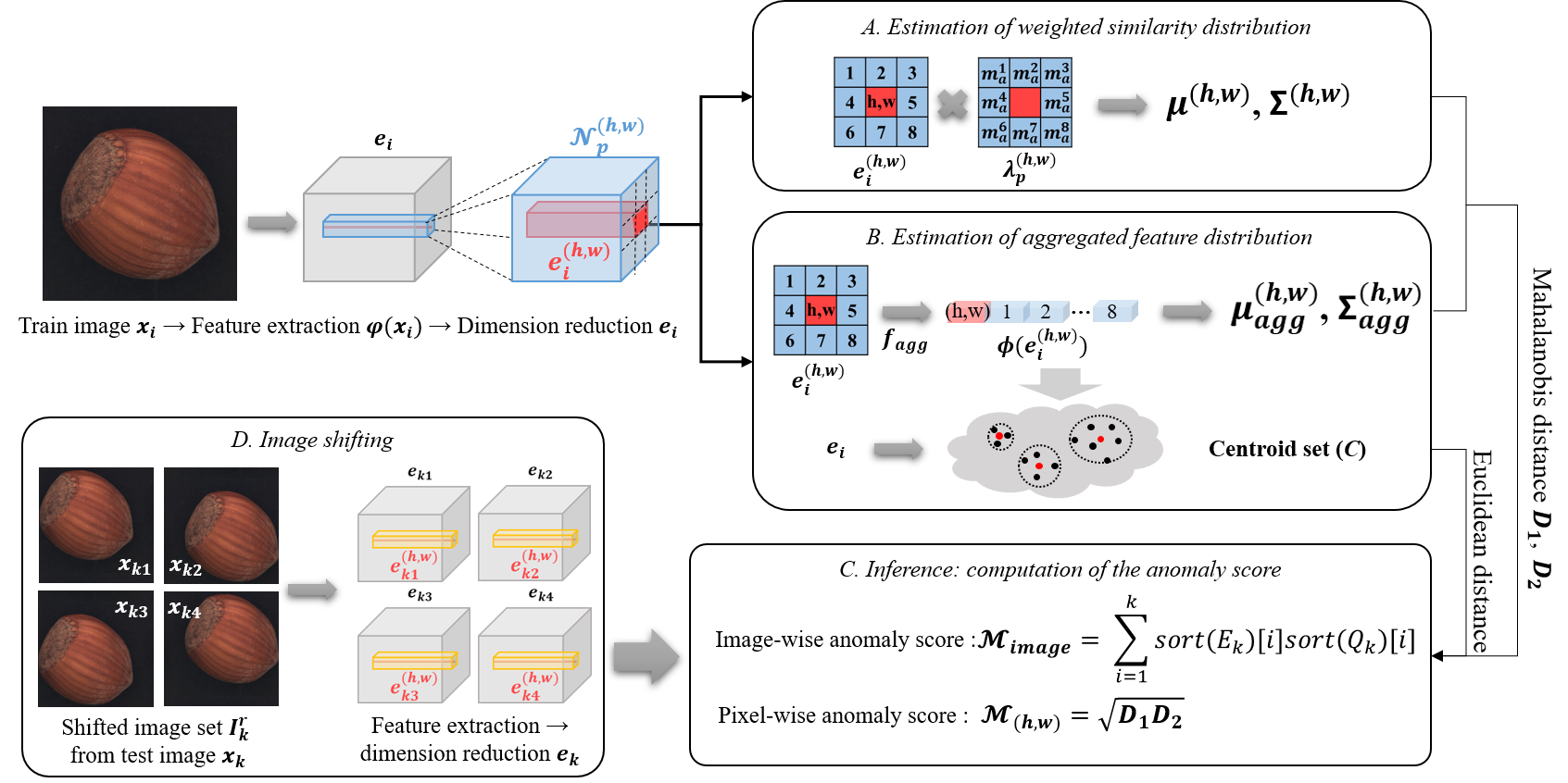
Figure 1: Overall model architecture. Two nominal distributions are estimated by applying the similarity between the target pixel and its neighboring pixels as weights (A) and by aggregating features of its neighborhood (B). Also, the k-means centroids of the aggregated features are identified as a set of representative nominal features for image-level detection (B). Next, the pixel-wise anomaly map and image-wise anomaly score are computed by Mahalonobis distances between the estimated distributions and test features and Euclidean distance between the centroids of train features and test features (C). Lastly, a shifting technique is applied to enhance the predictive performance (D).

3.1 Calculation of pixel-wise neighborhood similarity

Feature extraction In this study, a model architecture which implemented a pre-trained network on ImageNet as the backbone is designed for the out-of-distribution task of anomaly detection. Herein, the training set $\displaystyle\mathcal{X}_{train}=\{x_{k}\ |\ y_{k}=0\}$ consists of $\displaystyle|\mathcal{X}_{train}|=N$ nominal images, and the test set $\displaystyle\mathcal{X}_{test}=\{x_{k}\ |\ y_{k}=0\ or\ 1\}$ consists of $|\mathcal{X}_{test}|=N_{test}$ images that are either nominal or anomalous, where $x_{k}$ denotes a single image from a set of all images $\mathcal{X}_{train}$, and $y_{k}\in\{0,1\}$ denotes image $x_{k}$ as nominal with 0 and anomalous with 1. As in previous studies [8, 26, 9, 3], ResNet-like architectures, such as ResNet50 and WideResnet-50, were employed to extract feature maps. Within the given network $\varphi_{h}$, feature maps are extracted from the final output of the spatial resolution block at a specific hierarchy level $(h=1,2,3)$. Because the feature map extracted from the lowest hierarchy level $(h=1)$ has the largest size, the feature maps of higher hierarchy levels $(h=2,3)$ are interpolated to this size. Consequently, the pre-trained feature set $\varphi(x_{k})=[\varphi_{h}(x_{k})\ ,\ h=\{1,2,3\}]$ is constructed by concatenating all channels from each level.

Dimension Reduction Before estimating the nominal distributions, dimension reduction is performed on the total set of concatenated features $\varphi(x_{k})$ because features extracted from the pre-trained network may infer redundant information. Although the concatenated channels at each pixel are assumed to follow a multivariate Gaussian distribution, not every channel may follow a Gaussian distribution. In this sense, when reducing the number of channels, we aim to select the channels with an approximate Gaussian distribution form. We believe that the normal distribution may be distorted when all channels with values below zero are set to zero after applying ReLU function at the end of most pre-trained networks. Accordingly, the nonzero values in the nominal features are counted for each channel, and the top-$d$ channels with the least nonzero values are selected. Consequently, the final nominal feature set reduced from $\varphi(x_{k})$ is identified and denoted as $e_{x_{k}}$.

3.2 Estimation of weighted similarity distribution

Calculation of pixel-wise neighbor Bhattacharyya distance To estimate the nominal distribution at each pixel, we propose a novel method for computing the pixel-wise similarity between a pixel and its neighborhood. In this study, we aim to calibrate possible misalignments by including information from neighboring pixels, whereas the perfect alignment of pixels was essential for position-based estimations in existing methods. Specifically, the neighborhood of a pixel is defined as the set of $p$ pixels that were adjacent to the target pixel:

$$\begin{split}\displaystyle\mathcal{N}_{p}^{(h,w)}=\{(h^{\prime},w^{\prime})\ |\ h^{\prime}&\in\ [h-\lfloor p/2\rfloor,h+\lfloor p/2\rfloor],\\ \ w^{\prime}&\in\ [w-\lfloor p/2\rfloor,w+\lfloor p/2\rfloor]\}\end{split}$$ (1)

First, based on the assumption that every pixel $(h,w)$ in a feature map $e_{i}^{\left(h,w\right)}$ of a nominal image $i$ follows a multivariate Gaussian distribution, the sample mean $\mu^{\left(h,w\right)}$ and covariance $\Sigma^{\left(h,w\right)}$ of the nominal distribution are estimated. In addition, a regularization term $\epsilon I$ is added to $\Sigma^{\left(h,w\right)}$ to ensure full rank and invertibility.

$$\displaystyle\mu^{\left(h,w\right)}=\frac{1}{N}\sum_{i=1}^{N}e_{i}^{\left(h,w\right)}$$ (2)

$$\Sigma^{\left(h,w\right)}\!=\frac{1}{N\!\!-\!\!1}\!\!\sum_{i=1}^{N}\!{\left(e_{i}^{\left(h,w\right)}-\mu^{\left(h,w\right)}\right)\!\!\!\left(e_{i}^{\left(h,w\right)}-\mu^{\left(h,w\right)}\right)\!^{T}}\!\!\!+\!\epsilon I$$ (3)

Next, the Bhattacharyya distance $m$, which indicates the distance between two probability distributions, is computed between the target pixel and all pixels within the neighborhood. Because the Bhattacharyya coefficient $BC$ measures the overlapping degree of the two distributions, the negative exponential value of the coefficient is accepted as the similarity value. Consequently, the Bhattacharyya distance set $\lambda_{p}^{(h,w)}$ between the estimated distribution of pixels $(h,w)$, and $\mathcal{N}_{p}^{(h,w)}$ is computed as follows:

$$\lambda_{p}^{(h,w)}=\{m_{a}|a\in\mathcal{N}_{p}^{(h,w)}\}$$

$$\begin{split}&\displaystyle m_{a}=Batt(\mathcal{N}_{(\mu^{(h,w)},\Sigma^{(h,w)})},\mathcal{N}_{(\mu^{a},\Sigma^{a})}),Batt=e^{-\frac{BC}{\gamma}}\\ &\displaystyle BC(\mathcal{N}(\mu_{1},\Sigma_{1}),\mathcal{N}(\mu_{2},\Sigma_{2}))=\\ &\frac{1}{8}(\mu_{1}-\mu_{2})^{T}\Sigma^{\prime(-1)}\left(\mu_{1}-\mu_{2}\right)+\frac{1}{2}\log(\frac{det\Sigma^{\prime}}{\sqrt{det\Sigma_{1}det\Sigma_{2}}})\end{split}$$ (4)

where $\mu_{1}$ and $\mu_{2}$ denote a pair of mean values obtained from the estimated distributions and $\Sigma^{\prime}$ denotes the average of $\Sigma_{1}$ and $\Sigma_{2}$. Herein, a balancing parameter $\gamma$ is employed to modulate the degree to which the neighboring pixels are used to estimate the distributions. A $\gamma$ of 1 is equal to the original formulation of the Bhattacharyya distance, and larger values of $\gamma$ imply that more information is used from the neighborhood. Moreover, by assuming that the inherent information of pixels within a neighborhood, denoted as the sample covariances of $(h,w)$ and $(h’,w’)$, are similar, the logarithm of the ratio of the determinant terms in Eq. 4 is negligible. Consequently, the final similarity with the reduced computational cost is calculated as follows:

$$BC(\mathcal{N}_{(\mu_{1},\Sigma_{1})},\mathcal{N}_{(\mu_{2},\Sigma_{2})})\simeq\frac{1}{8}(\mu_{1}-\mu_{2})^{T}\Sigma^{\prime(-1)}\left(\mu_{1}-\mu_{2}\right)$$ (5)

Learning the normality based on similarity As the last step for learning the nominal distribution of each pixel, we aim to accentuate the features at specific locations that may infer more relevant information about the target pixel $(h,w)$. In this sense, weights are applied to the neighboring pixels according to their similarity to the target pixel. Accordingly, the similarity values calculated within $\mathcal{N}_{p}^{(h,w)}$ are utilized to estimate the weighted sample mean ${\bm{\mu}}^{(h,w)}$ and covariance ${\bm{\Sigma}}^{(h,w)}$ to accurately train the distribution of each pixel from the nominal images. The weighted sample mean and covariance are defined as follows:

$$\begin{split}\displaystyle{\bm{\mu}}^{(h,w)}=&\frac{1}{N}\sum_{i=1}^{N}\sum_{a\in\mathcal{N}_{p}^{(h,w)}}m_{a}^{\prime}e_{i}^{a},\ m_{a}^{\prime}=\frac{m_{a}}{\sum_{a\in\mathcal{N}_{p}^{(h,w)}}m_{a}}\\ \displaystyle{\bm{\Sigma}}^{(h,w)}=&\frac{1}{N-\sum_{a\in\mathcal{N}_{p}^{(h,w)}}(m_{a}^{\prime})^{2}}\times\\ &\sum_{i=1}^{N}\sum_{a\in\mathcal{N}_{p}^{(h,w)}}m_{a}^{\prime}(e_{i}^{a}-{\bm{\mu}}^{(h,w)})(e_{i}^{a}-{\bm{\mu}}^{(h,w)})^{T}\end{split}$$ (6)

3.3 Estimation of aggregated feature distribution

Learning the normality based on neighborhood aggregate features To best use the information of neighboring pixels, the normality based on aggregating neighborhood features (B in Fig. 1) is learned, in addition to the normality learned with weights (A in Fig. 1). Because neighboring pixels infer unseen information from the target pixel, an anomaly map for a receptive field with higher resolution is identified by aggregating the features within a neighborhood as follows:

$$\phi(e^{(h,w)})=f_{agg}(e^{a}|a\in\mathcal{N}_{p}^{(h,w)})$$ (7)

where $f_{agg}$ is the aggregation function for the neighborhood $\mathcal{N}_{p}^{(h,w)}$. In N-pad, we use adaptive average pooling for $f_{agg}$. Accordingly, the pixel-wise nominal distribution is learned by computing the sample mean and variance of the aggregated features at each pixel.

Because utilizing the Euclidean distance between the test feature and aggregated features has been effective in image-level anomaly detection in existing studies, we aim to construct a memory bank consisting of a group of essential features. In this sense, the aggregated features from the nominal set are clustered using k-means, and the features identified as the centroid of each cluster are grouped into a representative set of features denoted as $C$. In fact, the method of retrieving centroids as key features has been highly robust for outliers and noisy features within the nominal set and reported significant performance as opposed to arbitrary feature selection [11, 38, 41]. Thus, within the memory bank of all cluster centroids $C$, a group of centroids near the target feature is retrieved for image-level anomaly detection.

3.4 Inference: computation of anomaly score

Pixel-wise anomaly map The anomaly score of a pixel $(h,w)$ is computed using the Mahalanobis distance between the target pixel and distributions estimated by the two modules, in which features highly deviated from the nominal distributions reported higher anomaly scores.

First, because the information of neighboring pixels at $(h,w)$ is involved in estimating the weighted distribution of $\mathcal{N}({\bm{\mu}},{\bm{\Sigma}})$, features extracted at $(h,w)$ affect the values in $\mathcal{N}_{p}^{(h,w)}$. In this sense, we also employ the distributions of neighboring pixels when computing the anomaly score of the targeted position. Accordingly, Mahalanobis distances are computed between the target feature $e^{(h,w)}$ and its neighborhood, which is defined as a collection of estimated distributions $\mathcal{P}_{q}(e^{(h,w)})$ identified from $\mathcal{N}_{q}^{(h,w)}$. By applying a minimum aggregation function $f$ to the set of Mahalanobis distances, $\mathcal{D}_{1}$ is obtained for each pixel and used to calculate the anomaly score. The computation of $\mathcal{D}_{1}$ proceeds as follows:

$$\mathcal{P}_{q}(e^{(h,w)})=\{\mathcal{N}({{\bm{\mu}}^{a}},{\bm{\Sigma}}^{a})\ |\ a\ \in\ \mathcal{N}_{q}^{(h,w)}\}$$ (8)

$$\begin{split}\displaystyle&\mathcal{D}_{1}(e^{(h,w)},\mathcal{P}_{q}(e^{(h,w)}))=\\ &f(\sqrt{({e^{(h,w)}})-{\bm{\mu}}^{a})^{T}({\bm{\Sigma}}^{a})^{-1}(({e^{(h,w)}})-{\bm{\mu}}^{a})}\ |\ a\in\mathcal{N}_{q}^{(h,w)})\end{split}$$ (9)

Next, the Mahalanobis distance $\mathcal{D}_{2}$ between aggregated features $\phi(e^{(h,w)})$ of pixel $(h,w)$ and $\mathcal{N}({\bm{\mu}}_{agg}^{(h,w)},{\bm{\Sigma}}_{agg}^{h,w})$ is defined as follows:

$$\begin{split}&\displaystyle\mathcal{D}_{2}(\phi({e^{(h,w)}}),\mathcal{N}({\bm{\mu}}_{agg}^{(h,w)},{\bm{\Sigma}}_{agg}^{h,w}))=\\ &\sqrt{(\phi({e^{(h,w)}})-{\bm{\mu}}_{agg}^{(h,w)})^{T}({\bm{\Sigma}}_{agg}^{(h,w)})^{-1}(\phi({e^{(h,w)}})-{\bm{\mu}}_{agg}^{(h,w)})}\end{split}$$ (10)

Finally, to equalize the effects of the two pixel-wise anomaly maps $\mathcal{D}_{1}$ and $\mathcal{D}_{2}$ obtained from all pixels using Eq. 9 and Eq. 10, the geometric mean of the two maps is used as the final anomaly score $\mathcal{M}_{(h,w)}$:

$$\mathcal{M}_{(h,w)}=\sqrt{\mathcal{D}_{1}\mathcal{D}_{2}}$$ (11)

Image-wise anomaly score The image-level anomaly score based on the Euclidean distance between the aggregated features of a test image and refined set of aggregated nominal features has been effective in existing studies. Herein, a combination of Euclidean and Mahalanobis distances is employed to detect image-level anomalies more accurately. First, the top-$k$ Mahalanobis distances $\mathcal{D}_{1}$ between the target feature $e^{(h,w)}$ and estimated distribution collection of $\mathcal{P}_{q}(e^{(h,w)})$ are identified as a set $\mathcal{Q}_{k}$. Next, for all pixels included in $\mathcal{Q}_{k}$, the minimum Euclidean distance $d$ between the aggregated feature of a pixel $\phi(e^{v})$ and the centroids in set $C$ is calculated for all pixels and denoted as set $E_{k}$. Consequently, the image-level anomaly score is defined as follows:

$$\mathcal{Q}_{k}={\max_{(h,w)}}{k}(\mathcal{D}_{1}(e^{(h,w)},\mathcal{P}_{q}(e^{(h,w)})))$$ (12)

$$E_{k}=\{\min_{C}{d(\phi(e^{v}),C)}\ for\ \forall\ v\ \in\ \operatorname*{arg\,max}_{k}\mathcal{D}_{1}\}$$ (13)

$$\mathcal{M}_{image}=\sum_{i=1}^{k}sort(E_{k})[i]sort(\mathcal{Q}_{k})[i]$$ (14)

where $E_{k}$ and $\mathcal{Q}_{k}$ are sorted in ascending order because the sizes of the two distance values at each pixel are not in accordance. Consequently, employing both the top-$k$ Euclidean and Mahalanobis distances is demonstrated to be robust for computing image-level anomalies.

Image-shifting As the final inference step, target image $x_{k}$ is shifted by the pixel level from size 1 to $r$ to compute the final image-wise anomaly score and pixel-wise anomaly map based on the anomaly scores of the shifted images. By aggregating the scores from all shifted images of $x_{k}$ denoted as a set $\mathcal{I}_{k}^{r}$, we expect the marginal misalignment in the images to be negligible. Set $\mathcal{I}_{k}^{r}$ is defined as follows:

$$\begin{split}\displaystyle\mathcal{I}_{k}^{r}=\{x’_{k}\ |&\ x’_{k}[h-a,w-b]=x_{k}[h,w]\ \\ &\forall(a,b)\in[\lfloor-r/2,r/2\rfloor,\lfloor-r/2,r/2\rfloor]\}\end{split}$$ (15)

4 Experiments

4.1 Dataset and experimental setup

In this study, the proposed model is trained and evaluated on MVTec Anomaly Detection dataset (MVTec-AD) [5], which has been widely used for industrial anomaly detection tasks in existing studies. MVTec-AD consists of ten object and five texture classes with 3,629 nominal-only images for training and 1,725 nominal and anomalous images for evaluation. Moreover, we perform additional experiments Magnetic Tile Defects (MTD) in the Appendix to further validate our model. All images are center-cropped from 256 × 256 to 224 × 224 before model training and evaluation. The proposed model with a neighborhood size $p$ of 3 for model training, neighborhood size $q$ of 2 for inference, shift size $r$ of 4, balancing parameter $\gamma$ of 0.25, dimension reduction to 550, and 10% use of the centroids from $C$ reported the best predictive performance.

To evaluate the performance of the proposed model, the image and pixel levels of the AUROC are measured. In addition to the AUROC, the per-region-overlap score (PRO-score), which has been widely used in existing studies to measure anomaly detection performance, is measured for pixel-level anomaly segmentation [5, 6]. Herein, a PRO-curve is plotted using the average rates of correctly classified pixels for all connected anomalous components, with the false positive rates set between 0 and 0.3. Accordingly, the PRO-score is computed by normalizing the area under the PRO-curve.

Method	Normalizing Flow Based			Pre-trained Feature Based
Class/Model	FastFlow	PEFM	CFLOW-AD	SPADE	PaDiM	PatchCore	N-pad
Bottle	100/98.10	100/98.11	100/98.14	- /98.4	-/98.3	100/98.6	100/98.91
Cable	97.58/96.98	98.95/96.58	97.41/96.70	-/97.2	-/96.7	99.4/98.5	99.54/98.88
Capsule	98.52/98.84	91.90/97.94	97.69/98.64	-/99.0	-/98.5	97.8/98.9	99.40/98.96
Carpet	99.15/98.95	100/99.00	99.04/98.99	-/97.5	-/99.1	98.7/99.1	99.27/99.03
Grid	99.68/99.24	96.57/98.48	96.24/96.76	-/93.7	-/97.3	97.9/98.7	98.67/98.13
Hazelnut	97.96/97.62	99.89/98.78	100/98.35	-/99.1	-/98.2	100/98.7	100/99.03
Leather	100/99.41	100/99.24	100/99.36	-/97.6	-/99.2	100/99.3	100/99.43
Metalnut	99.51/98.36	99.85/96.89	98.92/98.32	-/98.1	-/97.2	100/98.4	100/99.19
Pill	98.22/97.64	97.51/96.67	96.92/98.70	-/96.5	-/95.7	96.0/97.6	98.00/99.04
Screw	86.34/98.48	96.43/98.93	83.95/97.74	-/98.9	-/98.5	97.0/99.4	97.40/98.80
Tile	100/96.45	99.49/95.19	100/97.30	-/87.4	-/94.1	98.9/95.9	100/97.62
Toothbrush	89.16/97.87	96.38/98.28	92.78/98.27	-/97.9	-/98.8	99.7/98.7	100/99.00
Transistor	98.58/97.07	97.83/96.58	97.38/93.15	-/94.1	-/98.5	100/96.4	99.58/98.55
Wood	99.56/96.23	99.19/95.27	99.30/94.80	-/88.5	-/94.9	99.0/95.1	99.56/97.49
Zipper	98.55/99.04	98.03/98.29	99.03/98.38	-/96.5	-/98.5	99.5/98.9	99.34/99.16
Average	97.52/98.03	98.13/97.61	97.24/97.57	-/96.0	-/97.5	99.0/98.1	99.37/98.75

Table 1: Image- and pixel-wise AUROC comparison of various models on MVTec-AD dataset

Model	FastFlow	PEFM	CFLOW-AD	SPADE	PaDiM	PatchCore	N-pad
PRO-score	93.0	92.4	91.7	91.7	92.1	93.5	95.1
Error	7.0	7.6	8.3	8.3	7.9	6.5	4.9

Table 2: PRO-score of different approaches on the MVTec-AD dataset

4.2 Comparison with baseline methods

To validate the predictive performance of the proposed model, we have benchmarked methods from general anomaly detection, pre-trained feature-based models, and existing models with state-of-the-art performance on MVTec-AD dataset. Since some existing models, such as Cflow-AD and PEFM, reported ensembled results with different image resolutions or without the 224 X 224 crop, we standardize the image size of all models prior to model training for objective comparison.

Tab. 1 presents the AUROC of image-level anomaly detection and pixel-level anomaly segmentation for all 15 classes of MVTec-AD. Herein, the proposed model consistently outperforms existing models with state-of-the-art-performance in both tasks. Specifically, the reduction of error for image-level detection is 37% compared to the pre-trained feature-based model of PatchCore. Moreover, the proposed model achieves state-of-the-art performance in pixel-wise AUROC for 12 out of 15 classes with an average AUROC of 98.75 and PRO-score of 95.1 (Tab. 2), reducing the error by 34% and 25%, respectively, compared to the next best performing model.

We believe that the proposed method of applying similarity between the target pixel and its neighborhood as weights successfully trained the underlying relationship within the pixels. In addition, we believe that the shifting module also contributed greatly to the predictive performance by inferring the distributions of neighboring pixels when computing anomaly score. Considering that identifying ill-produced samples is highly essential and demanding in industrial fields, our experiments have demonstrated that the proposed model may be effective in industrial anomaly detection.

4.3 Ablation study

Evaluation of the effectiveness of key design components The effectiveness of the four modules comprising the proposed model architecture (A, B, C, and D in Fig. 1) is evaluated by removing certain modules and comparing their predictive performances. Herein, five experiments are performed, as follows.

Experiment 1: Inference only using the weighted similarity distribution of the target pixel without the aggregated feature distribution (A).

Experiment 2: Inference only using the aggregated feature distribution without the weighted similarity distributions (B).

Experiment 3: Inference using both the weighted similarity distribution of the target pixel and aggregated feature distribution (A+B).

Experiment 4: Inference using the distributions from neighboring pixels to estimate the weighted similarity distribution (A+C).

Experiment 5: Inference using the distributions from neighboring pixels to estimate the weighted similarity and aggregated feature distributions without shifting (A+B+C).

Method	Exper1	Exper2	Exper3	Exper4	Exper5	N-pad
Pixel-wise AUROC	98.38	98.45	98.59	98.57	98.65	98.75
Error	1.62	1.58	1.41	1.43	1.35	1.25

Table 3: Evaluation of the effectiveness of key design components

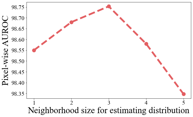
(a) AUROC comparison of different neighborhood sizes ($p$) for estimating distribution

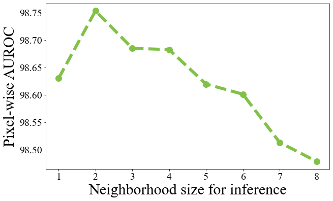
(b) AUROC comparison of different neighborhood sizes ($q$) for inference

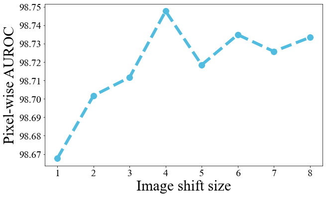
(c) AUROC comparison of different image shift sizes ($r$)

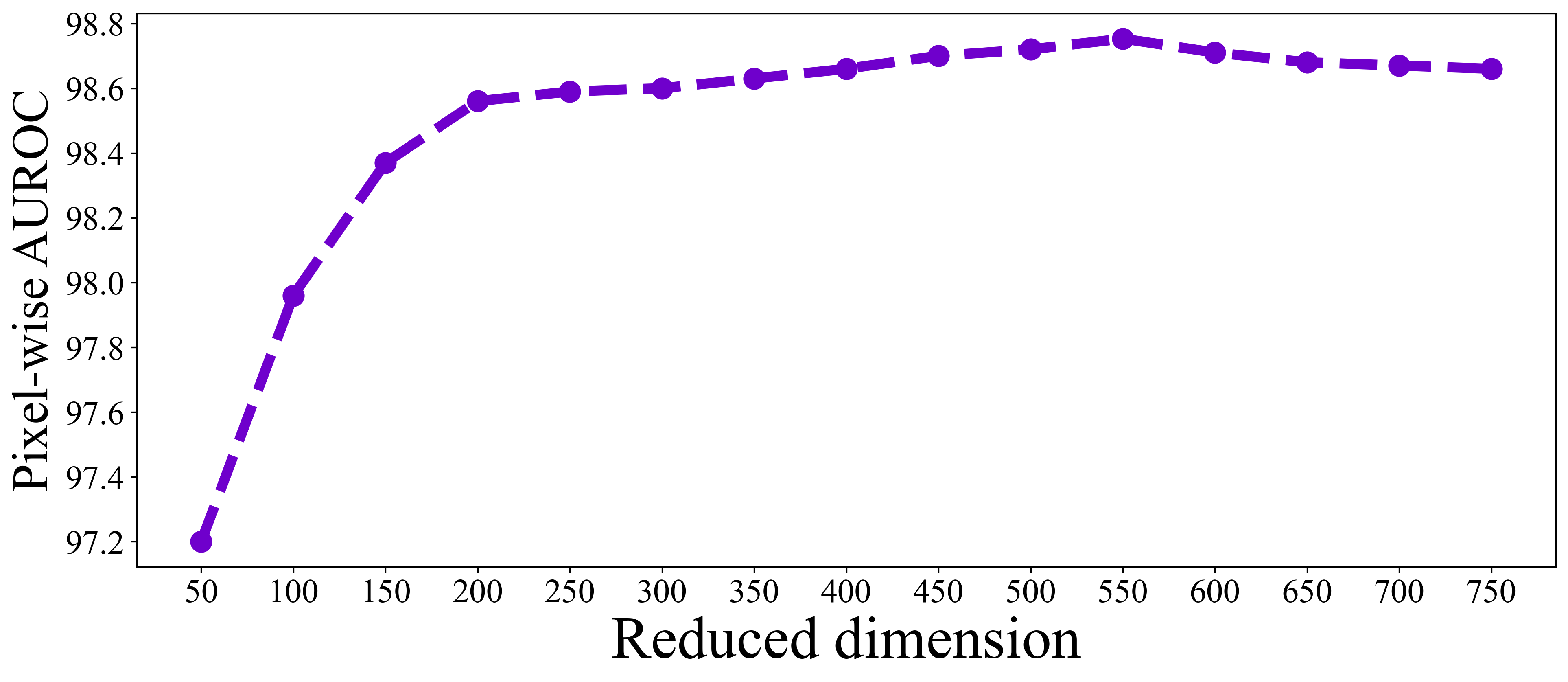
(d) AUROC comparison of different dimension reduction

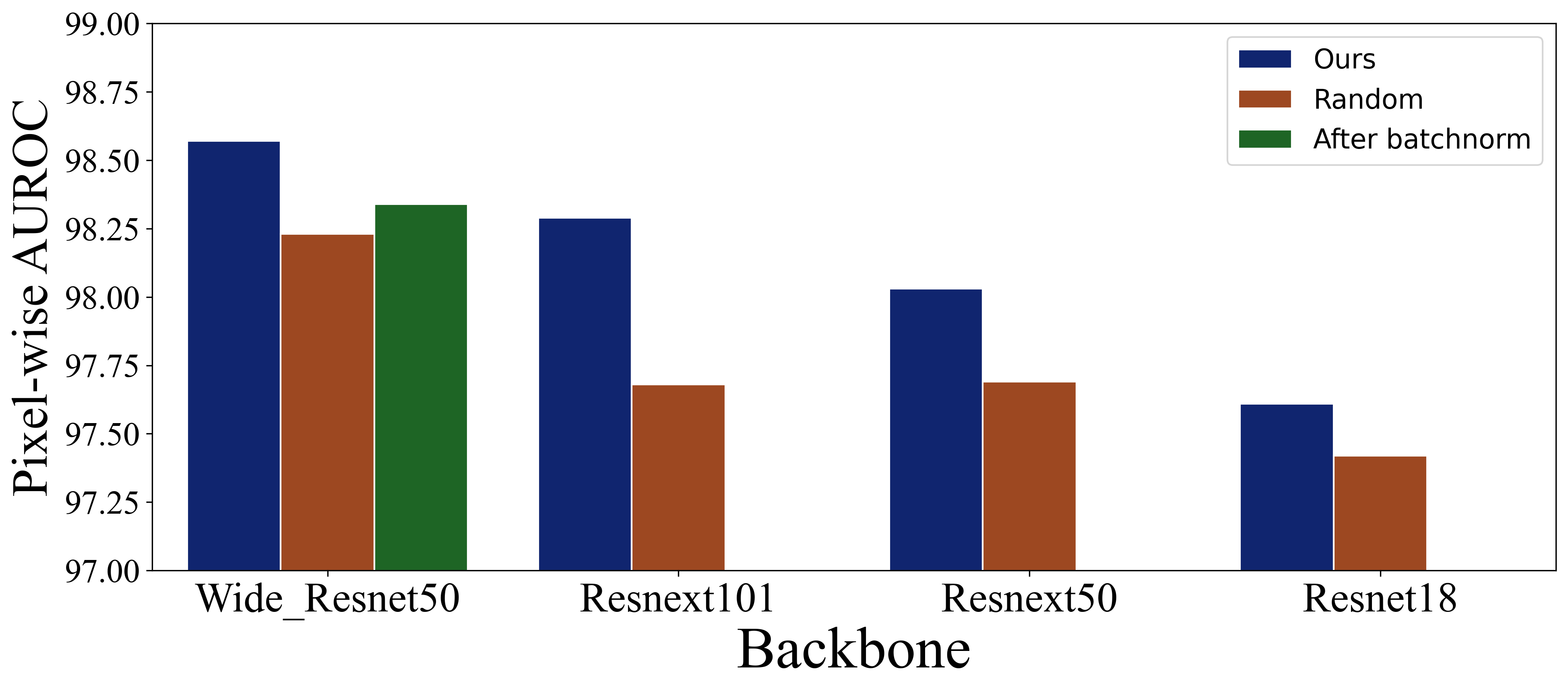
(e) AUROC comparison of different backbones

Figure 2: Verification of parameter efficiency with various sizes and backbones.

Tab. 3 shows that all modules significantly contribute to the performance of anomaly detection. First, the degraded performance in Experiment 5 compared with the result of N-pad proves that shifting the aggregated anomaly maps is superior to the sole use of the original images. Next, 0.19 increase in the AUROC from Experiment 1 to Experiment 4 demonstrates that using the distributions from the neighboring pixels was effective in estimating the weighted similarity distribution. This result suggests that aggregating the anomaly scores computed from the distributions of neighboring pixels is effective. Finally, the improved performance in Experiment 3, which integrated both modules from Experiments 1 and 2, demonstrates that the inference that uses both weighted similarity and aggregated feature distributions was effective.

Verification of parameter efficiency in model architecture Various parameters within the modules were tested to determine the optimal design of the proposed model. First, different neighborhood sizes ($p$) for estimating the distributions of weighted similarity or aggregated features are tested. Fig. 2(a) demonstrates that the performance improves as the neighborhood size increases from 1, reaches the optimal level at a size of 3, and degrades with larger sizes. Thus, we believe that acquiring information from considerably close neighbors is the best, whereas distant neighbors infer excessive information with no greater relevance to the target pixel.

Second, the different numbers of distributions on neighboring pixels ($q$) used to compute the anomaly map in module A (Fig. 1) are tested. Fig. 2(b) shows a neighbor size of 2 as the optimal value. Because applying a large neighborhood size may affect numerous pixels of the original image during interpolation, we believe that a relatively small number is optimal.

Third, different shifting sizes ($r$) are tested, as shown in Fig. 2(c), resulting in a shifting size of 4 being the most optimal. This approach demonstrates that calibrating imperfectly aligned industrial images through the aggregation of slightly shifted versions of the images can significantly contribute to improved performance.

Fourth, the number of channels following the dimension reduction is tested by first using 50 channels and increasing the number up to 550 in units of 50. As shown in Fig. 2(d), the proposed model outperforms PatchCore, a state-of-the-art model, with an pixel-wise AUROC of 98.1, when the number reaches 150 channels, which is only 8.37% of the total number of channels. Because the computational cost reduces quadratically with fewer channels, this result demonstrates that the proposed model can be effective with minimal computation.

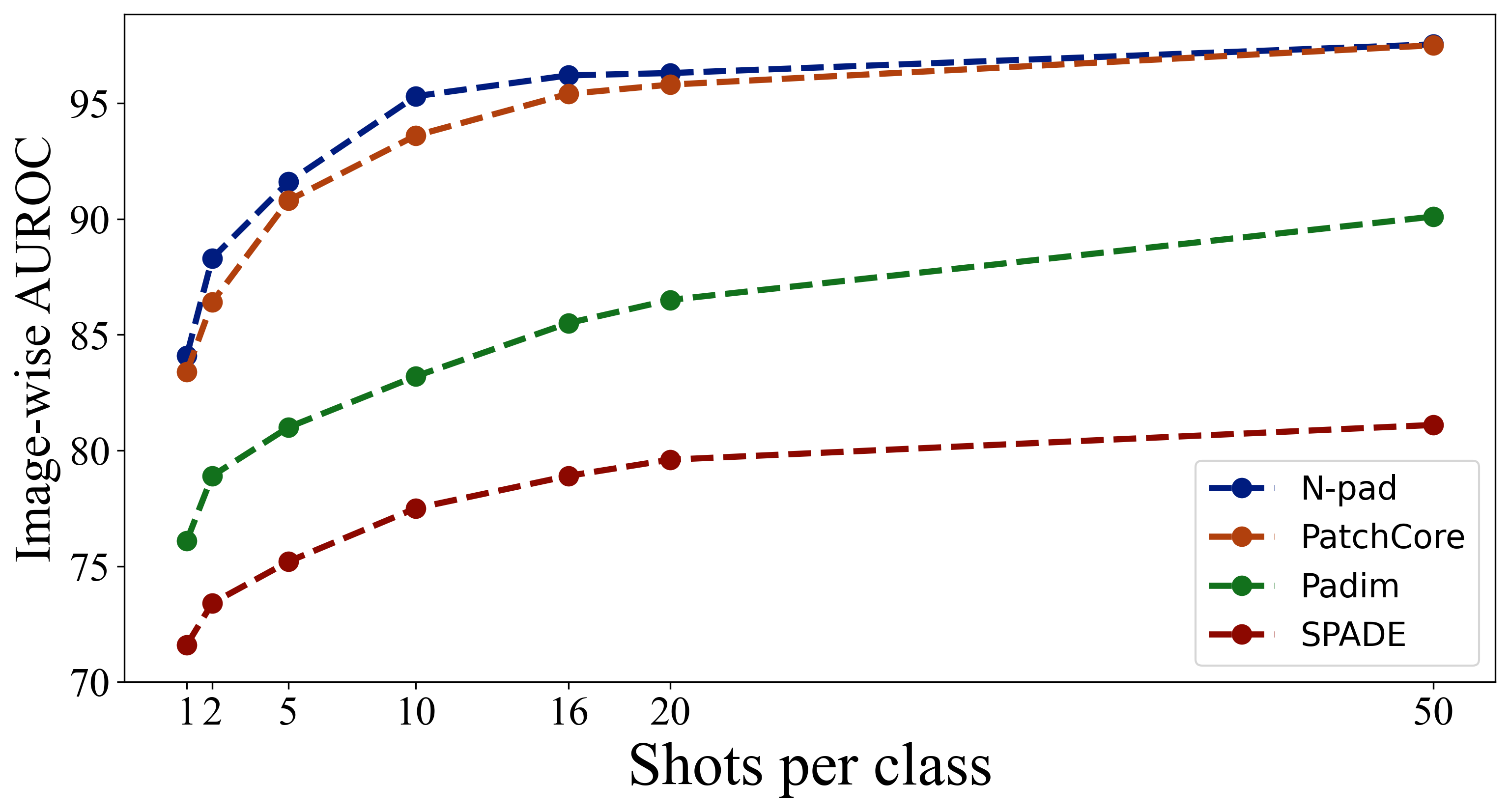
(a) Image-wise AUROC comparison of different models.

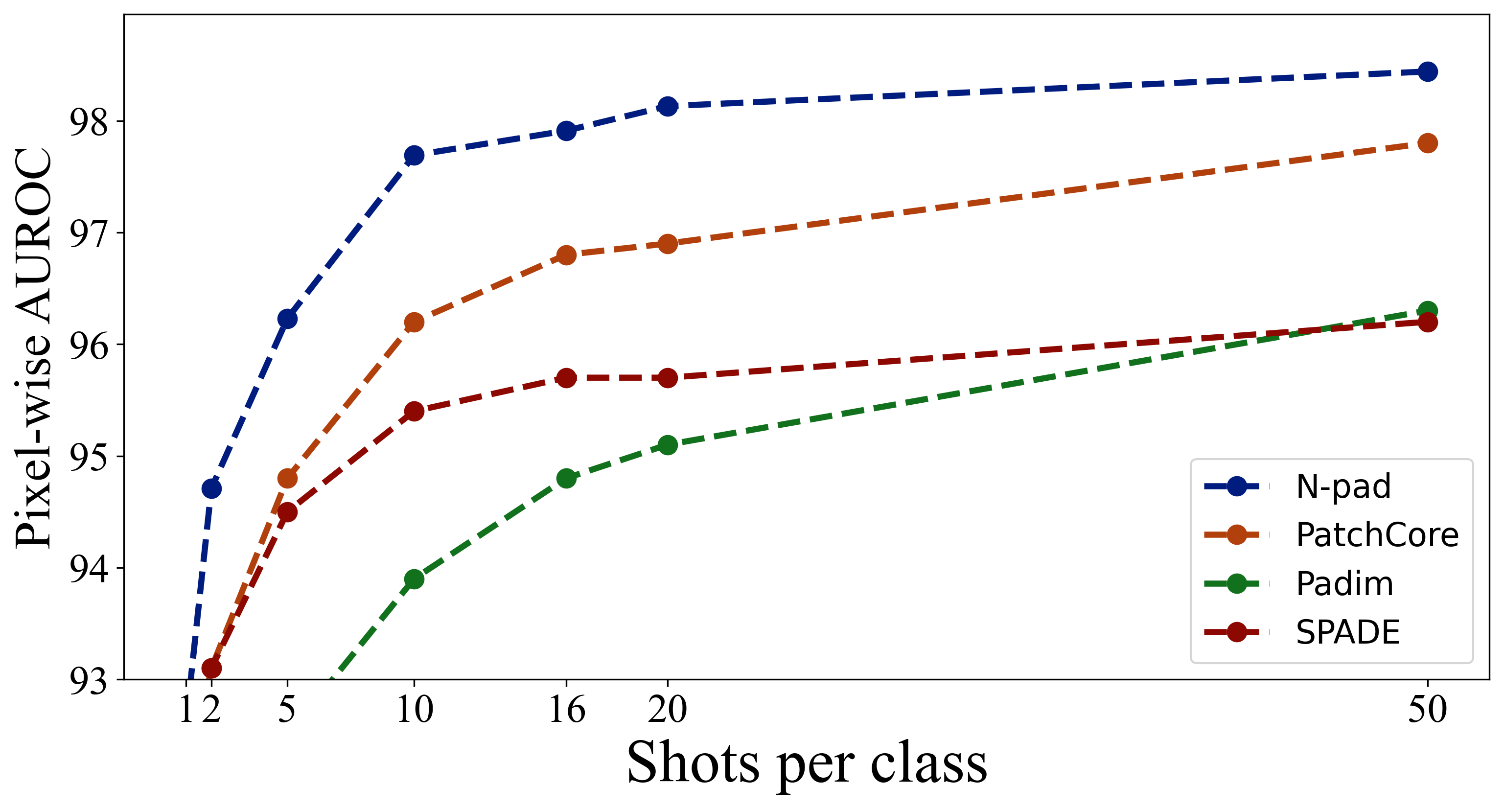
(b) Pixel-wise AUROC comparison of different models.

Figure 3: Few shot anomaly detection performance

Finally, additional experiments are performed with different image sizes because a few existing models have reported benchmark scores by extensively reshaping the image size or excluding image crops. Because the cropped area is mostly the edge of the image background, which may be easily identified as nominal pixels, the better predictive performance is recorded with larger image sizes without cropping. Consequently, an ensemble of models which employed images cropped by 224 and 336 reported the best pixel-wise AUROC of 98.98, as shown in Tab. 4.

Method	256Resize 224crop	256Resize	320Resize 280Crop	384Resize 336Crop	Ensemble
Pixel-wise AUROC	98.75	98.91	98.86	98.89	98.98

Table 4: AUROC comparison of different image sizes and crops

Evaluation of the effectiveness of Bhattacharyya distance for estimating weighted similarity distributions To demonstrate the effectiveness of the Bhattacharyya distance calculation for estimating the weighted similarity distributions in this study, uniform and random weights are tested for comparison, as presented in Tab. 5. First, weights that are randomly applied resulted in poor performance because the relationships within the pixels were not considered. Moreover, uniformly applied weights also have a minimal effect on the estimated mean and covariance of the distributions, because features from neighboring pixels may not infer significantly different information from the target pixel. Consequently, the proposed method of weighted sampling based on similarity is reported as the most effective for predictive performance.

Sampling Method	1/n	Random	Ours
Pixel-wise AUROC	98.42	98.42	98.45

Table 5: AUROC comparison of different sampling methods

Comparison of methods for reducing dimensions with various backbones To evaluate the proposed distribution-based method for dimension reduction, results based on a random dimension reduction with different backbones are reported for comparison. First, the random selection of dimensions in the proposed model achieves an AUROC decrease of 0.34. Next, a random dimension reduction in features extracted at the batch normalization layer prior to ReLU scores AUROC that is 0.23 lower than that of the proposed model. This result demonstrates that because the channels activated greater than 0 by the activation function are more relevant for ImageNet classification, the pre-trained network features extracted from those channels may have been more effective. Furthermore, various model architectures other than the WideResNet-50 of the proposed model, such as ResNet18, ResNext50, WideResNet-101, and ResNext-101, are tested for comparison. As shown in Fig. 2(e), the proposed method reports a better performance than random reduction in all architectures, demonstrating the consistency of its superiority.

4.4 Few-shot Anomaly Detection

Few-shot anomaly detection In the industrial field, anomaly detection can be required for initial production, where only a small set of nominal sample data is available. Accordingly, few-shot anomaly detection is performed to test the proposed model with limited nominal data by testing the number of training images from 1 to 50. Consequently, the proposed model achieves better performance than the previous state-of-the-art model using only 8% of the total dataset. Because the proposed model employs information from neighboring pixels to train the distribution of the target pixel, the augmented information from the neighborhood may have significantly contributed to few-shot learning.

5 Conclusion

In this paper, we propose a novel model for industrial anomaly detection and segmentation that utilizes features from the neighborhood of the target pixel. We estimate the nominal distribution of each pixel inferring the the information in the neighborhood by applying the similarity between the neighboring pixels and target pixel as weights. Moreover, another estimation of the nominal distribution based on aggregated features is proposed to employ information from various receptive fields. Various experiments evaluate the model in multiple settings and achieved state-of-the-art performances on the 15 classes of an industrial anomaly dataset. Thus, we believe that learning nominal distributions with the pre-trained features of neighboring pixels is useful and effective for improving predictive performances in industrial anomaly detection.

Appendix

Appendix A Evalution on MTD dataset

In addition to the MVTec-AD dataset, we performed additional experiments with MTD (Magnetic Tile Defects) dataset which has also been used for industrial anomaly detection in previous studies[16]. MTD dataset consists of magnetic tile images in various shapes and patterns, of which 925 are nominal and 392 are anomalous. As in previous studies, 80% of the nominal data were employed for model training and the remaining 20% and the anomalous data were employed for evaluation. Accordingly, the results were compared to existing pre-trained network-based models and DifferNet[27], which reported good performance. The results are reported as follows:

Model	DifferNet	PaDiM	PatchCore	N-pad
Image-wise AUROC	97.7	86.88	97.9	98.22
Pixel-wise AUROC		82.45	84.90	85.43

Table 6: Evalution on MTD dataset

Since the shapes of nominal data are not consistent, the images may not be clearly aligned, which makes the predictions on MTD dataset challenging. Nevertheless, we have achieved superior performance by employing neighboring pixels to calculate anomaly score.

Appendix B Evaluation on various ratios of k-means centroids

We have tested various ratios of the K-means centroids included for model evaluation and compared their AUROCs. In fact, the decrease in the number of clusters did not significantly affect the results because a highly robust set of centroids was employed.

K-means ratio	0.25	0.1	0.05	0.01	0.005
Image-wise AUROC	99.39	99.37	99.34	99.31	99.10

Table 7: Evaluation of image-wise AUROC on various ratios of k-means centroids

Model/Class	Bottle	Cable	Capsu.	Carpet	Grid	Hazel.	Leat.	Metal.	Pill	Screw	Tile	Tooth.	Trans.	Wood	Zip.	Average
FastFlow	91.9	89.6	92.7	96.3	97.4	94.5	99.1	93.4	92.4	92.6	89.1	83.6	91.7	93.0	96.7	93.0
CFLOW	93.2	92.6	93.9	95.3	89.5	95.3	98.5	90.2	94.4	91.7	86.8	85.7	84.7	90.4	93.1	91.7
PEFM	95.4	93.7	93.4	96.3	94.8	95.5	98.3	93.1	95.2	94.7	81.5	89.0	79.9	90.3	95.1	92.4
SPADE	95.5	90.9	93.7	94.7	86.7	95.4	97.2	94.4	94.6	96.0	75.6	93.5	87.4	87.4	92.6	91.7
PaDIM	94.8	88.8	93.5	96.2	94.6	92.6	97.8	85.6	92.7	94.4	86.0	93.1	84.5	91.1	95.9	92.1
PatchCore	96.1	92.6	95.5	96.6	95.9	93.9	98.9	91.3	94.1	97.9	87.4	91.4	83.5	89.6	97.1	93.5
N-pad	96.3	97.2	95.7	95.6	94.2	95.6	97.2	95.1	97.1	94.9	89.8	93.7	94.5	93.4	97.1	95.1

Table 8: PRO Score comparison of various models on MVTec-AD dataset

Appendix C Details in PRO-score

PRO-scores of each class in the MVTec-AD, which have not been listed in detail in Sec. 4.2, are reported in Tab. 8. Here, N-pad reported the best performance in terms of PRO score for 11 out of 15 classes of MVTec-AD. Specifically, previous models reported higher scores only for carpet, grid, screw, and zipper. Thus, we may suggest that the proposed model has been developed with superior performance.

Appendix D Visual result

We present pixel-wise anomaly maps of several anomalous images for all classes in MVTec-AD that were computed by PaDiM, PatchCore and N-pad in Figs. 4, 5 and 6. Herein, pixel-wise anomaly maps were visualized by normalizing the anomaly scores from 20% to 80% to eliminate relatively nominal pixels and emphasize the anomalous regions. The results are as follows:

Figure 4: Visualization anomalies from top to bottom: bottle, cable, capsule, carpet, and grid.

Figure 5: Visualization anomalies from top to bottom: hazelnut, leather, metalnut, pill, and screw.

Figure 6: Visualization anomalies from top to bottom: tile, toothbrush, transistor, wood and zipper.

References

- [1] Pankaj K Agarwal, Sariel Har-Peled, Kasturi R Varadarajan, et al. Geometric approximation via coresets. Combinatorial and computational geometry, 52(1), 2005.
- [2] Samet Akcay, Amir Atapour-Abarghouei, and Toby P Breckon. Ganomaly: Semi-supervised anomaly detection via adversarial training. In Asian conference on computer vision, pages 622–637. Springer, 2018.
- [3] Liron Bergman, Niv Cohen, and Yedid Hoshen. Deep nearest neighbor anomaly detection. arXiv preprint arXiv:2002.10445, 2020.
- [4] Liron Bergman and Yedid Hoshen. Classification-based anomaly detection for general data. arXiv preprint arXiv:2005.02359, 2020.
- [5] Paul Bergmann, Michael Fauser, David Sattlegger, and Carsten Steger. Mvtec ad–a comprehensive real-world dataset for unsupervised anomaly detection. In Proceedings of the IEEE/CVF conference on computer vision and pattern recognition, pages 9592–9600, 2019.
- [6] Paul Bergmann, Michael Fauser, David Sattlegger, and Carsten Steger. Uninformed students: Student-teacher anomaly detection with discriminative latent embeddings. In Proceedings of the IEEE/CVF Conference on Computer Vision and Pattern Recognition (CVPR), June 2020.
- [7] Paul Bergmann, Sindy Löwe, Michael Fauser, David Sattlegger, and Carsten Steger. Improving unsupervised defect segmentation by applying structural similarity to autoencoders. In VISIGRAPP (5: VISAPP), 2019.
- [8] Niv Cohen and Yedid Hoshen. Sub-image anomaly detection with deep pyramid correspondences. arXiv preprint arXiv:2005.02357, 2020.
- [9] Thomas Defard, Aleksandr Setkov, Angelique Loesch, and Romaric Audigier. Padim: a patch distribution modeling framework for anomaly detection and localization. In International Conference on Pattern Recognition, pages 475–489. Springer, 2021.
- [10] Hanqiu Deng and Xingyu Li. Anomaly detection via reverse distillation from one-class embedding. In Proceedings of the IEEE/CVF Conference on Computer Vision and Pattern Recognition, pages 9737–9746, 2022.
- [11] Thanh-Toan Do, Toan Tran, Ian Reid, Vijay Kumar, Tuan Hoang, and Gustavo Carneiro. A theoretically sound upper bound on the triplet loss for improving the efficiency of deep distance metric learning. In Proceedings of the IEEE/CVF Conference on Computer Vision and Pattern Recognition, pages 10404–10413, 2019.
- [12] Eleazar Eskin, Andrew Arnold, Michael Prerau, Leonid Portnoy, and Sal Stolfo. A geometric framework for unsupervised anomaly detection. In Applications of data mining in computer security, pages 77–101. Springer, 2002.
- [13] Izhak Golan and Ran El-Yaniv. Deep anomaly detection using geometric transformations. Advances in neural information processing systems, 31, 2018.
- [14] Dong Gong, Lingqiao Liu, Vuong Le, Budhaditya Saha, Moussa Reda Mansour, Svetha Venkatesh, and Anton van den Hengel. Memorizing normality to detect anomaly: Memory-augmented deep autoencoder for unsupervised anomaly detection. In Proceedings of the IEEE/CVF International Conference on Computer Vision, pages 1705–1714, 2019.
- [15] Denis Gudovskiy, Shun Ishizaka, and Kazuki Kozuka. Cflow-ad: Real-time unsupervised anomaly detection with localization via conditional normalizing flows. In Proceedings of the IEEE/CVF Winter Conference on Applications of Computer Vision, pages 98–107, 2022.
- [16] Yibin Huang, Congying Qiu, and Kui Yuan. Surface defect saliency of magnetic tile. The Visual Computer, 36(1):85–96, 2020.
- [17] Longin Jan Latecki, Aleksandar Lazarevic, and Dragoljub Pokrajac. Outlier detection with kernel density functions. In International Workshop on Machine Learning and Data Mining in Pattern Recognition, pages 61–75. Springer, 2007.
- [18] Kimin Lee, Kibok Lee, Honglak Lee, and Jinwoo Shin. A simple unified framework for detecting out-of-distribution samples and adversarial attacks. Advances in neural information processing systems, 31, 2018.
- [19] Sungwook Lee, Seunghyun Lee, and Byung Cheol Song. Cfa: Coupled-hypersphere-based feature adaptation for target-oriented anomaly localization. arXiv preprint arXiv:2206.04325, 2022.
- [20] Wenqian Liu, Runze Li, Meng Zheng, Srikrishna Karanam, Ziyan Wu, Bir Bhanu, Richard J Radke, and Octavia Camps. Towards visually explaining variational autoencoders. In Proceedings of the IEEE/CVF Conference on Computer Vision and Pattern Recognition, pages 8642–8651, 2020.
- [21] Prasanta Chandra Mahalanobis. On the generalized distance in statistics. National Institute of Science of India, 1936.
- [22] Pramuditha Perera, Ramesh Nallapati, and Bing Xiang. Ocgan: One-class novelty detection using gans with constrained latent representations. In Proceedings of the IEEE/CVF Conference on Computer Vision and Pattern Recognition, pages 2898–2906, 2019.
- [23] Stanislav Pidhorskyi, Ranya Almohsen, and Gianfranco Doretto. Generative probabilistic novelty detection with adversarial autoencoders. Advances in neural information processing systems, 31, 2018.
- [24] Tal Reiss, Niv Cohen, Liron Bergman, and Yedid Hoshen. Panda: Adapting pretrained features for anomaly detection and segmentation. In Proceedings of the IEEE/CVF Conference on Computer Vision and Pattern Recognition, pages 2806–2814, 2021.
- [25] Oliver Rippel, Patrick Mertens, and Dorit Merhof. Modeling the distribution of normal data in pre-trained deep features for anomaly detection. In 2020 25th International Conference on Pattern Recognition (ICPR), pages 6726–6733. IEEE, 2021.
- [26] Karsten Roth, Latha Pemula, Joaquin Zepeda, Bernhard Schölkopf, Thomas Brox, and Peter Gehler. Towards total recall in industrial anomaly detection. In Proceedings of the IEEE/CVF Conference on Computer Vision and Pattern Recognition, pages 14318–14328, 2022.
- [27] Marco Rudolph, Bastian Wandt, and Bodo Rosenhahn. Same same but differnet: Semi-supervised defect detection with normalizing flows. In Proceedings of the IEEE/CVF winter conference on applications of computer vision, pages 1907–1916, 2021.
- [28] Lukas Ruff, Robert Vandermeulen, Nico Goernitz, Lucas Deecke, Shoaib Ahmed Siddiqui, Alexander Binder, Emmanuel Müller, and Marius Kloft. Deep one-class classification. In International conference on machine learning, pages 4393–4402. PMLR, 2018.
- [29] Lukas Ruff, Robert A Vandermeulen, Nico Görnitz, Alexander Binder, Emmanuel Müller, Klaus-Robert Müller, and Marius Kloft. Deep semi-supervised anomaly detection. In International Conference on Learning Representations, 2019.
- [30] Mohammad Sabokrou, Mohammad Khalooei, Mahmood Fathy, and Ehsan Adeli. Adversarially learned one-class classifier for novelty detection. In Proceedings of the IEEE conference on computer vision and pattern recognition, pages 3379–3388, 2018.
- [31] Mayu Sakurada and Takehisa Yairi. Anomaly detection using autoencoders with nonlinear dimensionality reduction. In Proceedings of the MLSDA 2014 2nd workshop on machine learning for sensory data analysis, pages 4–11, 2014.
- [32] Thomas Schlegl, Philipp Seeböck, Sebastian M Waldstein, Ursula Schmidt-Erfurth, and Georg Langs. Unsupervised anomaly detection with generative adversarial networks to guide marker discovery. In International conference on information processing in medical imaging, pages 146–157. Springer, 2017.
- [33] Kihyuk Sohn, Chun-Liang Li, Jinsung Yoon, Minho Jin, and Tomas Pfister. Learning and evaluating representations for deep one-class classification. In International Conference on Learning Representations, 2020.
- [34] Jihoon Tack, Sangwoo Mo, Jongheon Jeong, and Jinwoo Shin. Csi: Novelty detection via contrastive learning on distributionally shifted instances. Advances in neural information processing systems, 33:11839–11852, 2020.
- [35] Chin-Chia Tsai, Tsung-Hsuan Wu, and Shang-Hong Lai. Multi-scale patch-based representation learning for image anomaly detection and segmentation. In Proceedings of the IEEE/CVF Winter Conference on Applications of Computer Vision, pages 3992–4000, 2022.
- [36] Shashanka Venkataramanan, Kuan-Chuan Peng, Rajat Vikram Singh, and Abhijit Mahalanobis. Attention guided anomaly localization in images. In European Conference on Computer Vision, pages 485–503. Springer, 2020.
- [37] Qian Wan, Cao YunKang, Liang Gao, Shen Weiming, and Xinyu Li. Position encoding enhanced feature mapping for image anomaly detection. In 2022 IEEE 18th International Conference on Automation Science and Engineering (CASE), 2022.
- [38] Jixuan Wang, Kuan-Chieh Wang, Marc T Law, Frank Rudzicz, and Michael Brudno. Centroid-based deep metric learning for speaker recognition. In ICASSP 2019-2019 IEEE International Conference on Acoustics, Speech and Signal Processing (ICASSP), pages 3652–3656. IEEE, 2019.
- [39] Jihun Yi and Sungroh Yoon. Patch svdd: Patch-level svdd for anomaly detection and segmentation. In Proceedings of the Asian Conference on Computer Vision, 2020.
- [40] Jiawei Yu, Ye Zheng, Xiang Wang, Wei Li, Yushuang Wu, Rui Zhao, and Liwei Wu. Fastflow: Unsupervised anomaly detection and localization via 2d normalizing flows. arXiv preprint arXiv:2111.07677, 2021.
- [41] Ye Yuan, Wuyang Chen, Yang Yang, and Zhangyang Wang. In defense of the triplet loss again: Learning robust person re-identification with fast approximated triplet loss and label distillation. In Proceedings of the IEEE/CVF Conference on Computer Vision and Pattern Recognition Workshops, pages 354–355, 2020.
- [42] Bo Zong, Qi Song, Martin Renqiang Min, Wei Cheng, Cristian Lumezanu, Daeki Cho, and Haifeng Chen. Deep autoencoding gaussian mixture model for unsupervised anomaly detection. In International conference on learning representations, 2018.