Effects of Emerging Bipolar Magnetic Regions in Mean-field Dynamo Model of Solar Cycles 23 and 24

Abstract

We model the physical parameters of Solar Cycles 23 and 24 using a nonlinear dynamical mean-field dynamo model that includes the formation and evolution of bipolar magnetic regions (BMR). The Parker-type dynamo model consists of a complete MHD system in the mean-field formulation: the 3D magnetic induction equation, and 2D momentum and energy equations in the anelastic approximation. The initialization of BMR is modeled in the framework of Parker’s magnetic buoyancy instability. It defines the depths of BMR injections, which are typically located at the edge of the global dynamo waves. The distribution with longitude and latitude and the size of the initial BMR perturbations are taken from the NOAA database of active regions. The modeling results are compared with various observed characteristics of the solar cycles. Only the BMR perturbations located in the upper half of the convection zone lead to magnetic active regions on the solar surface. While the BMR initialized in the lower part of the convection zone do not emerge on the surface, they still affect the global dynamo process. Our results show that BMR can play a substantial role in the dynamo processes, and affect the strength of the solar cycle. However, the data-driven model shows that the BMR effect alone cannot explain the weak Cycle 24. This weak cycle and the prolonged preceding minimum of magnetic activity were probably caused by a decrease of the turbulent helicity in the bulk of the convection zone during the decaying phase of Cycle 23.

1 Introduction

The basic scenario for the hydromagnetic solar dynamo involves a cyclic mutual transformation of the toroidal and poloidal magnetic fields by means of differential rotation and cyclonic convective motions characterized by kinetic helicity (Parker, 1955). The key idea of Parker suggests that the poloidal magnetic field of the Sun is generated from rising loops of the toroidal magnetic field in the deep convection zone, which are twisted around the radial direction by turbulent cyclonic motions (“the alpha-effect”). The resulting poloidal fields of the loops coalesce into a large-scale poloidal magnetic field of a new solar cycle. The subsequent stretching of the poloidal field by the differential rotation produces the toroidal field (“the Omega-effect”). The whole 22-year cyclic process of the magnetic field generation and transformation represents dynamo waves, forming the magnetic butterfly diagram and reversing the magnetic polarity of the Sun’s global magnetic field. Occasional strands of toroidal flux tubes emerge on the surface due to the magnetic buoyancy instability (Parker, 1955, 1979) in the form of east-west oriented Bipolar Magnetic Regions (BMR).

On the one hand, this scenario stems from the turbulent dynamo theory and mean-field dynamo models (Moffatt, 1978; Parker, 1979; Raedler, 1980), which are the basis of our current understanding of the nature of magnetic activity in astrophysical objects (Brandenburg & Subramanian, 2005; Shukurov & Subramanian, 2021). Global convective MHD simulations prove the validity of the basic principles of the dynamo theory (Guerrero et al., 2016; Schrinner, 2011; Schrinner et al., 2011; Warnecke et al., 2018, 2021). Naturally, the mean-field solar dynamo models consider the dynamo process to be distributed over the convection zone and ‘shaped’ into the butterfly diagram of emerged BMR in the subsurface rotational shear layer (Brandenburg, 2005; Pipin & Kosovichev, 2011a).

On the other hand, the phenomenological scenario of Babcock-Leighton (hereafter, BL) (Babcock, 1961; Leighton, 1969), based on observations of magnetic field evolution on the solar surface, grew into a popular flux-transport model of the solar cycles (see reviews by Charbonneau, 2011; Brun et al., 2014; Dikpati, 2016). In this scenario, the poloidal field is generated due to the latitudinal tilt of BMR emerging on the solar surface. This field is transported by the surface meridional circulation and turbulent diffusion to the polar regions where it sinks in the interior and is amplified by the differential rotation, creating a new toroidal field, which produces emerging BMR. The meridional circulation speed controls the solar-cycle duration. For these dynamo models, the surface magnetic activity, which is often considered in the form of an empirical “source term” in the induction equation, is crucial.

In terms of the mean-field theory, the empirical Babcock-Leighton source term calculated from the magnetic flux of BMR observed on the solar surface can be considered as a near-surface alpha-effect (Stix, 1974). From this point of view, the primary differences between Parker’s and Babcock-Leighton’s scenarios are in the distribution of the alpha-effect in the convection zone and the role of the turbulent magnetic diffusion and meridional circulation in the magnetic flux transport. While Parker’s scenario assumes that the alpha-effect is distributed in the convection zone and turbulent diffusion plays a major role in the formation of migrating dynamo waves and considers the formation of BMR as a secondary effect, in the Babcock-Leighton scenario, the BMR play a key role providing the surface alpha-effect and magnetic flux transported by the meridional circulation to the polar regions.

Theoretical models based on these scenarios have been successful in explaining some observed properties of the solar cycles and magnetic field evolution. The Babcock-Leighton flux-transport models explain the magnetic flux emergence and transport observed on the solar surface as well as the evolution of the polar magnetic field (Dikpati et al., 2016). The recently developed self-consistent Parker-type mean-field model (Pipin, 2018) explains the global magnetic structure and evolution (Obridko et al., 2021), as well as the dynamical processes, such as the migrating zonal flows – torsional oscillations (Kosovichev & Pipin, 2019) and variations of the meridional circulation (Getling et al., 2021), observed by helioseismology. The model also explained the extended solar-cycle phenomenon (Pipin & Kosovichev, 2019). This model determines the 3D evolution of the large-scale vector magnetic field, coupled with the equations describing large-scale flows and heat transport in the axisymmetric 2D approximation. Thus, unlike in the Babcock-Leighton models, the differential rotation and meridional circulation are not input parameters - they are calculated together with the magnetic field evolution. This allowed comparing the model results with the helioseismic measurements.

Despite the recent advances, both types of dynamo models do not provide a clear understanding of the physical mechanisms causing variations of the solar amplitude and, thus, cannot provide robust solar-cycle predictions. In the Babcock-Leighton models, the primary idea is that the solar cycle strength is governed by spatial and temporal variations of the BMR tilt, which affects the amount of magnetic flux transported to the polar regions (e.g. Dikpati, 2016). On the other hand, Parker-type models attempt to explain the solar-cycle amplitudes by long- and short-term variations of the distributed alpha-effect and associated non-linear processes in the deep convection zone (e.g. Pipin & Kosovichev, 2020).

To evaluate the role of BMR in these models, Pipin (2022) developed a 3D mean-field model, which includes the mechanism of magnetic flux emergence due to the magnetic buoyancy instability resulting in the formation of BMR on the surface. It was found that the generation of the large-scale poloidal field via the emergence and evolution of the solar bipolar magnetic regions can profoundly effect on the global dynamo process. Thus, this new type of mean-field dynamo modeling includes the basic features of both Parker’s and Babcock-Leighton’s scenarios.

In this paper, we study the effects of BMR on the solar dynamo using the mean-field dynamo model of Pipin & Kosovichev (2020) and the BMR formulation of Pipin (2022). Our aim is to investigate the global parameters of the mean-field dynamo for these solar cycles and evaluate the role of BMR in the cycle properties. To model the surface magnetic activity, we adopt the data of solar active regions from the NOAA Space Weather Prediction Center for Solar Cycles 23 and 24. In particular, we study the evolution of the polar magnetic field and investigate whether the modeled BMR activity can explain the weak Cycle 24.

2 Model formulation

The model is formulated within the mean-field MHD (magnetohydrodynamics) framework of Krause & Rädler (1980). The basic details of the model are given earlier by Pipin & Kosovichev (2019) (hereafter PK19) and Pipin (2022) (hereafter, P22).

The magnetic field evolution is governed by the mean-field induction equation:

$$\partial_{t}\left\langle\mathbf{B}\right\rangle=\mathbf{\nabla}\times\left(\mathbf{\mathbf{\boldsymbol{\mathbf{\mathcal{E}}}}+}\left\langle\mathbf{U}\right\rangle\times\left\langle\mathbf{B}\right\rangle\right)\,,$$ (1)

where $\mathbf{\mathcal{E}}=\left\langle\mathbf{u\times b}\right\rangle$ is the mean electromotive force; $\mathbf{u}$ and $\mathbf{b}$ are the turbulent fluctuating velocity and magnetic field, respectively; and $\left\langle\mathbf{U}\right\rangle$ and $\left\langle\mathbf{B}\right\rangle$ are the mean velocity and magnetic field. We assume that the averaging is done over the ensemble of turbulent flows and magnetic fields. We decompose the induction vector $\left\langle\mathbf{B}\right\rangle$ into the sum of the axisymmetric and non-axisymmetric parts,

$$\left\langle\mathbf{B}\right\rangle=\overline{\mathbf{B}}+\tilde{\mathbf{B}},$$ (2)

where $\overline{\mathbf{B}}$ and $\tilde{\mathbf{B}}$ are the axisymmetric and non-axisymmetric components of the large-scale magnetic field. The mean electromotive force describes the turbulent effects on the mean magnetic field evolution. It consists of two parts:

$$\mathcal{E}_{i} = \mathcal{E}_{i}^{(A)}+\mathcal{E}_{i}^{(\mathrm{BMR})},$$ (3)

where $\mathcal{E}_{i}^{(A)}$ is calculated analytically using the double-scale approximation of Roberts & Soward (1975) (see, e.g., Kitchatinov et al. 1994; Pipin 2008). The phenomenological part $\mathcal{E}_{i}^{(\mathrm{BMR})}$describes formations of the surface bipolar regions (BMR) from the large-scale toroidal magnetic field.

The expression for $\mathcal{E}_{i}^{(A)}$ reads as follows,

$$\mathcal{E}_{i}^{(A)}=\left(\alpha_{ij}+\gamma_{ij}\right)\left\langle B\right\rangle_{j}-\eta_{ijk}\nabla_{j}\left\langle B\right\rangle_{k},$$ (4)

here, $\alpha_{ij}$ describes the turbulent generation of the magnetic field by helical motions (the $\alpha$-effect), $\gamma_{ij}$ describes the turbulent pumping, and $\eta_{ijk}$ is the eddy magnetic diffusivity tensor. The $\alpha$-effect tensor includes the small-scale magnetic helicity density contribution, i.e., the pseudo-scalar $\left\langle\chi\right\rangle=\left\langle\mathbf{a}\cdot\mathbf{b}\right\rangle$ (where $\mathbf{a}$ and $\mathbf{b}$ are the fluctuating vector-potential and magnetic field, respectively),

$$\alpha_{ij} = C_{\alpha}\psi_{\alpha}(\beta)\alpha_{ij}^{(H)}+\alpha_{ij}^{(M)}\psi_{\alpha}(\beta)\frac{\left\langle\chi\right\rangle\tau_{c}}{4\pi\overline{\rho}\ell_{c}^{2}},$$ (5)

where the expressions of the kinetic helicity tensor $\alpha_{ij}^{(H)}$ and the magnetic helicity tensor $\alpha_{ij}^{(M)}$ are given by Pipin (2018). The radial profiles of the $\alpha_{ij}^{(H)}$ and $\alpha_{ij}^{(M)}$ depend on the mean density stratification, profile of the convective RMS velocity $u_{c}$ and on the Coriolis number $\Omega^{*}=2\Omega_{0}\tau_{c}$, where $\Omega_{0}$ is the angular velocity of the star and $\tau_{c}$ is the convective turnover time. The magnetic quenching function $\psi_{\alpha}(\beta)$ depends on the parameter $\mathrm{\beta=\left|\left\langle\mathbf{B}\right\rangle\right|/\sqrt{4\pi\overline{\rho}u_{c}^{2}}}$. Note that in the presence of the $\tilde{\mathbf{B}}$-field, the $\alpha$ effect tensor becomes non-axisymmetric. It is caused by the $\psi_{\alpha}(\beta)$-quenching and the magnetic helicity effects.

The magnetic helicity evolution follows the global conservation law for the total magnetic helicity, $\left\langle\chi\right\rangle^{(tot)}=\left\langle\chi\right\rangle+\left\langle\mathbf{A}\right\rangle\cdot\left\langle\mathbf{B}\right\rangle$, (see, Hubbard & Brandenburg (2012); Pipin et al. (2013); Brandenburg (2018)):

$$\left(\frac{\partial}{\partial t}+\boldsymbol{\left\langle\mathbf{U}\right\rangle\cdot\nabla}\right)\left\langle\chi\right\rangle^{(tot)}=-\frac{\left\langle\chi\right\rangle}{R_{m}\tau_{c}}-2\eta\left\langle\mathbf{B}\right\rangle\cdot\left\langle\mathbf{J}\right\rangle-\mathbf{\nabla\cdot}\mathbf{\mathbf{\mathcal{F}}}^{\chi},$$ (6)

where, we use ${\displaystyle 2\eta\mathbf{\left\langle b\cdot j\right\rangle}=\frac{\left\langle\chi\right\rangle}{R_{m}\tau_{c}}}$ (Kleeorin & Rogachevskii, 1999). Also, we introduce the diffusive flux of the small-scale magnetic helicity density, $\mathbf{\mathbf{\mathcal{F}}}^{\chi}=-\eta_{\chi}\mathbf{\nabla}\left\langle\chi\right\rangle$, and $R_{m}$ is the magnetic Reynolds number, we employ $R_{m}=10^{6}$. Following the results of Mitra et al. (2010), we put $\eta_{\chi}=\frac{1}{10}\eta_{T}$. Further details about the turbulent dynamo effects can be found in Pipin (2022)(P22) and in the above-cited papers. In what follows, we discard the advection of the total helicity by meridional circulation. As a result, the amplitude of the polar magnetic field in the mean-field model decreases in comparison to the standard case (cf, P22). One purpose of this tuning is to get a stronger impact of the surface BMR on the deep dynamo in the new model.

The turbulent pumping, which is expressed by the antisymmetric tensor $\gamma_{ij}$, is important for reproducing the solar-like evolution of the dynamo-generated magnetic field (Warnecke et al., 2014, 2021). The formulation of $\gamma_{ij}$ for the solar-type mean-field dynamo model was discussed by Pipin (2018). We define it as follows,

$$\gamma_{ij} = \gamma_{ij}^{(\Lambda\rho)}+\frac{\alpha_{\mathrm{MLT}}u_{c}}{\gamma}\mathcal{H}\left(\beta\right)\mathrm{\hat{r}_{n}\varepsilon_{inj}},$$ (7)

$$\gamma_{ij}^{(\Lambda\rho)} = 3\nu_{T}f_{1}^{(a)}\left\{\left(\mathbf{\boldsymbol{\Omega}}\cdot\boldsymbol{\Lambda}^{(\rho)}\right)\frac{\Omega_{n}}{\Omega^{2}}\varepsilon_{\mathrm{inj}}-\frac{\Omega_{j}}{\Omega^{2}}\mathrm{\varepsilon_{inm}\Omega_{n}\Lambda_{m}^{(\rho)}}\right\}$$ (8)

where $\mathbf{\boldsymbol{\Lambda}}^{(\rho)}=\boldsymbol{\nabla}\log\overline{\rho}$, $\mathrm{\alpha_{MLT}}=1.9$ is the mixing-length theory parameter, $\gamma$ is the adiabatic exponent, $u_{c}$ is the RMS convective velocity. In Eq.(7), the first term takes into account the mean drift of the large-scale field due to the gradient of the mean density, and the second term describes the magnetic buoyancy effect. Function $\mathcal{H}\left(\beta\right)$ takes into account the effect of magnetic tension. For small values of $\beta$, $\mathcal{H}\left(\beta\right)\sim\beta^{2}$, and it saturates as $\beta^{-2}$ for $\beta\gg 1$ (see P22 for details).

We assume that the large-scale flow is axisymmetric. It is decomposed into a sum of the meridional circulation and differential rotation, $\mathbf{\overline{U}}=\mathbf{\overline{U}}^{m}+r\sin\theta\Omega\left(r,\theta\right)\hat{\mathbf{\boldsymbol{\phi}}}$, where $r$ is the radial coordinate, $\theta$ is the polar angle, $\hat{\mathbf{\boldsymbol{\phi}}}$ is the unit vector in the azimuthal direction, and $\Omega\left(r,\theta\right)$ is the angular velocity profile. The angular momentum conservation and the equation for the azimuthal component of large-scale vorticity, $\mathrm{\overline{\omega}=\left(\boldsymbol{\nabla}\times\overline{\mathbf{U}}^{m}\right)_{\phi}}$, determine the differential rotation and meridional circulation:

$$\frac{\partial}{\partial t}\overline{\rho}r^{2}\sin^{2}\theta\Omega = -\boldsymbol{\nabla\cdot}\left(r\sin\theta\overline{\rho}\left(\hat{\mathbf{T}}_{\phi}+r\sin\theta\Omega\mathbf{\overline{U}^{m}}\right)\right)$$

$$+ \boldsymbol{\nabla\cdot}\left(r\sin\theta\frac{\left\langle\mathbf{B}\right\rangle\left\langle B_{\phi}\right\rangle}{4\pi}\right),$$

$$\mathrm{\frac{\partial\omega}{\partial t}} \mathrm{=} \mathrm{r\sin\theta\boldsymbol{\nabla}\cdot\left(\frac{\hat{\boldsymbol{\phi}}\times\boldsymbol{\nabla\cdot}\overline{\rho}\hat{\mathbf{T}}}{r\overline{\rho}\sin\theta}-\frac{\mathbf{\overline{U}}^{m}\overline{\omega}}{r\sin\theta}\right)}$$

$$+ \mathrm{r}\sin\theta\frac{\partial\Omega^{2}}{\partial z}-\mathrm{\frac{g}{c_{p}r}\frac{\partial\overline{s}}{\partial\theta}}$$

$$+ \frac{1}{4\pi\overline{\rho}}\left(\overline{\mathbf{B}}\boldsymbol{\cdot\nabla}\right)\left(\boldsymbol{\nabla}\times\overline{\mathbf{B}}\right)_{\phi}-\frac{1}{4\pi\overline{\rho}}\left(\left(\boldsymbol{\nabla}\times\overline{\mathbf{B}}\right)\boldsymbol{\cdot\nabla}\right)\overline{\mathbf{B}}{}_{\phi},$$

where $\hat{\mathbf{T}}$ is the turbulent stress tensor:

$$\hat{T}_{ij}=\left(\left\langle u_{i}u_{j}\right\rangle-\frac{1}{4\pi\overline{\rho}}\left(\left\langle b_{i}b_{j}\right\rangle-\frac{1}{2}\delta_{ij}\left\langle\mathbf{b}^{2}\right\rangle\right)\right),$$ (11)

(see detailed description in Pipin & Kosovichev, 2019, PK19). Also, $\overline{\rho}$ is the mean density, $\mathrm{\overline{s}}$ is the mean entropy; $\mathrm{\partial/\partial z=\cos\theta\partial/\partial r-\sin\theta/r\cdot\partial/\partial\theta}$ is the gradient along the axis of rotation. The mean heat transport equation determines the mean entropy variations from the reference state due to the generation and dissipation of large-scale magnetic fields and flows (Pipin & Kitchatinov, 2000):

$$\overline{\rho}\overline{T}\left(\frac{\partial\overline{\mathrm{s}}}{\partial t}+\left(\overline{\mathbf{U}}\cdot\boldsymbol{\nabla}\right)\overline{\mathrm{s}}\right)=-\boldsymbol{\nabla}\cdot\left(\mathbf{F}^{c}+\mathbf{F}^{r}\right)-\hat{T}_{ij}\frac{\partial\overline{U}_{i}}{\partial r_{j}}-\boldsymbol{\boldsymbol{\mathcal{E}}}\cdot\left(\nabla\times\left\langle\mathbf{B}\right\rangle\right),$$ (12)

where $\overline{T}$ is the mean temperature, $\mathbf{F}^{r}$ is the radiative heat flux, $\mathbf{F}^{c}$ is the anisotropic convective flux (see, PK19). The last two terms in Eq. (12) take into account the convective energy gain and sink caused by the generation and dissipation of large-scale magnetic and flow fields. The reference profiles of mean thermodynamic parameters, such as entropy, density, and temperature, are determined from the stellar interior model MESA (Paxton et al., 2011, 2013). The radial profile of the typical convective turnover time, $\tau_{c}$, is determined by the MESA code, as well. We assume that $\tau_{c}$ does not depend on the magnetic field and global flows. The convective RMS velocity is determined from the mixing-length approximation,

$$\mathrm{u_{c}=\frac{\ell_{c}}{2}\sqrt{-\frac{g}{2c_{p}}\frac{\partial\overline{s}}{\partial r}},}$$ (13)

where $\ell_{c}=\alpha_{MLT}H_{p}$ is the mixing length, $\alpha_{MLT}=1.9$ is the mixing-length parameter, and $H_{p}$ is the pressure scale height. Equation (13) determines the reference profiles for the eddy heat conductivity, $\chi_{T}$, eddy viscosity, $\nu_{T}$, and eddy diffusivity, $\eta_{T}$, as follows,

$$\chi_{T} = \frac{\ell^{2}}{6}\sqrt{-\frac{g}{2c_{p}}\frac{\partial\overline{s}}{\partial r}},$$ (14)

$$\nu_{T} = \mathrm{Pr}_{T}\chi_{T},$$ (15)

$$\eta_{T} = \mathrm{Pm_{T}\nu_{T}}.$$ (16)

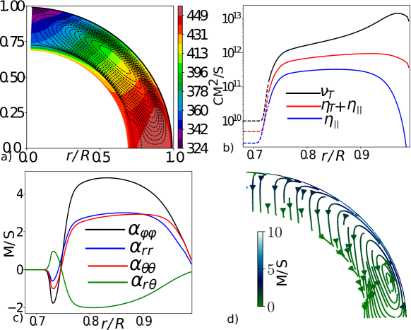
Figure 1: a) The meridional circulation (streamlines) and the angular velocity distributions; the magnitude of circulation velocity is $\sim 13$ m/s on the surface at 45^∘ latitude; b) radial dependencies of the total eddy magnetic diffusivity, $\eta_{T}+\eta_{||}$, and its rotationally induced part, $\eta_{||}$, and the eddy viscosity profile, $\nu_{T}$; c) the $\alpha$-effect tensor components as a function of radius at 45^∘ latitude; and d) the streamlines of the toroidal magnetic field effective drift velocity caused by the meridional circulation and the turbulent pumping effect. For post-processing of modeling data and visualization in this and other figures, we use numpy/scipy (Harris et al., 2020; Virtanen et al., 2020) together with matplotlib (Hunter, 2007) and pyvista (Sullivan & Kaszynski, 2019) .

Table 1: Basic parameters of the reference axisymmetric dynamo model, see explanation in the text.

hydrodynamic & heat transport	dynamo model & boundary condition parameters
$\alpha_{\mathrm{MLT}}=1.9$,$\ell_{\mathrm{min}}=0.01R$, $\mathrm{Pr}_{T}=3/4$	$C_{\alpha}=0.04$,$\mathrm{Pm}_{T}=10$, $\delta=0.999$, $B_{\mathrm{esq}}=5$G

The solution of the heat transport equation determines the mean entropy distribution. The entropy profile and the Coriolis number, $\Omega^{*}=2\Omega_{0}\tau_{c}$ define the magnitude and distribution of the turbulent effects in the convection zone. The profile of $\tau_{c}=\ell_{c}/u_{c}$ is taken from the output of the MESA code. For overshoot overshoot region we assume that the intensity of the turbulent mixing decays with exponent of $100$ from the bottom of the convection zone. We assume that the bottom of overshoot region rotates as a solid-body at the rate $\Omega_{0}=430$ nHz. The reference axisymmetric model has only a few free parameters. We choose them to fit the reference model into solar observations.

Firstly, for the distributed dynamo model the radial location of the meridional circulation stagnation point is important. If the stagnation point in the upper part of the convection zone then the latitudinal turbulent pumping together with the meridional circulation, and the Parker-Yoshimura law results into the solar-type dynamo waves of the large-scale toroidal field (Pipin 2018, 2021). The location of the stagnation point and meridional circulation structure depends on the $\Lambda$-effect profile in the solar convection zone. It is determined by the mean-field expression obtained by Kitchatinov & Rudiger (1993) and Kitchatinov (2004). In the standard mean-field models of solar differential rotation, e.g., the model of Kitchatinov & Rüdiger (2005), the $\Lambda$-effect is determined by the density gradient, turbulence anisotropy and the Coriolis number profile of the solar convection zone. The stagnation point of the meridional circulation in their model is located near the bottom of the convection zone. Similar to (Pipin & Kosovichev, 2018) our model takee into account the radial gradient of the convective turnover time, $\tau_{c}$ . This effects results to inversion of the $\Lambda$-effect near the bottom of the convection zone. It causes the origin of the second meridional circulation cell (clockwise in the North) near the bottom of the convection zone. Also the stagnation point of the main cell (anticlockwise in the North) is shifted toward the top in this case According to the convection zone properties given by the MESA code, $\tau_{c}$ increases sharply towards the bottom of convection zone. To get the model with one circulation cell and the stagnation point in the upper part of convection zone we smooth the sharp variation of $\tau_{c}$ toward the bottom of the convection zone using the following ansatz of Kitchatinov & Nepomnyashchikh (2017):

$$\ell_{c}=\ell_{\mathrm{min}}+\frac{1}{2}\left(\ell_{c}^{(0)}-\ell_{\mathrm{min}}\right)\left[1+\mathrm{erf}\left(\frac{r-(r_{b}+\ell_{\mathrm{min}})}{R_{\odot}d}\right)\right],$$ (17)

where $\ell_{c}^{(0)}$ is the mixing-length parameter from the MESA code, $r_{b}=0.728R_{\odot}$ is the radius of the bottom of the convection zone, $d=0.02$. We use $\ell_{\mathrm{min}}$ as a control parameter to model saturation of $\tau_{c}$ variations in the $\Lambda$-tensor. For $\ell_{\mathrm{min}}=0$ we get the double cell meridional circulation structure. Here, we use $\ell_{\mathrm{min}}=0.01R$. This model show one-cell meridional circulation structure with stagnation point at $0.9R$ and the better agreement of the angular velocity profile with helioseismology than the model with double cell meridional circulation structure. Yet, the nonlinear model shows a weak second cell near the bottom of the convection zone in this case (see, Pipin & Kosovichev 2019). The eddy heat conductivity and eddy viscosity coefficients. Also, we employ a standard choice to relate eddy heat conductivity an eddy viscosity $\mathrm{Pr}_{T}=3/4$.

Secondly, the full dynamo cycle period of $20$ years is reproduced if $\mathrm{Pm}_{T}=11$. The critical threeshold of the dimensionless $\alpha$-effect parameter is $C_{\alpha}=0.04$. Figure 1 illustrates distributions of the angular velocity, meridional circulation, the $\alpha$-effect, and the eddy diffusivity calculated for a nonmagnetic model. The amplitude of the meridional circulation on the surface is about $13$ m/s. We list the critical parameters in the Table 1. The efffect of the boundary condition parameters will be discussed in subsection 2.3.

2.1 Formation of Bipolar Magnetic Regions (BMR)

Following ideas of Parker (1955, 1971), the emergence of the bipolar magnetic regions (BMR) is modeled by using the mean electromotive force representing the magnetic buoyancy and twisting effects acting on unstable parts of the axisymmetric magnetic field as follows (P22):

$$\mathcal{E}_{i}^{(\mathrm{BMR})}=\alpha_{\beta}\delta_{i\phi}\left\langle B\right\rangle_{\phi}+V_{\beta}\left(\hat{\boldsymbol{r}}\times\left\langle\mathbf{B}\right\rangle\right)_{i},$$ (18)

where the first term describes the $\alpha$-effect caused by the BMR tilt, and the second term models the magnetic buoyancy instability. The magnetic buoyancy velocity, $V_{\beta}$, includes the turbulent and mean-field buoyancy effects (Kitchatinov & Rüdiger, 1992; Kitchatinov & Pipin, 1993; Ruediger & Brandenburg, 1995):

$$V_{\beta} = \frac{\alpha_{\mathrm{MLT}}u_{c}}{\gamma}\mathcal{H}\left(\beta_{m}\right)\xi_{\beta}(t,\boldsymbol{r})$$ (19)

where function $\mathcal{H}\left(\beta\right)$ describes magnetic tension, $\mathrm{\beta=\left|\left\langle\mathbf{B}\right\rangle\right|/\sqrt{4\pi\overline{\rho}u_{c}^{2}}}$, and subscript ’m’ marks unstable points. Function $\xi_{\beta}$, defines the location and formation of the unstable part of the magnetic field,

$$\!\xi_{\beta}^{(\pm)}\left(\boldsymbol{r},t\right)\! = C_{\beta}\negthinspace\tanh\mathrm{\left(\frac{t}{\tau_{0}}\right)}\exp\left(-m_{\beta}\left(\sin^{2}\!\left(\!\frac{\phi-\phi_{m}}{2}\!\right)\right.\right.\!$$

$$\left.\left.+\!\sin^{2}\!\left(\!\frac{\theta-\theta_{\mathrm{m}}}{2}\!\right)\!\right)\right)\psi(r,r_{m}^{(\pm)}),\,t<\delta\mathrm{t_{0}}$$

$$= 0,\,t>\delta t.$$

where $\psi$ is a kink type function of radius,

$$\psi(r,r_{m}^{(\pm)})\! =\!\! \frac{1}{4}\left(\!1\!+\!\mathrm{erf}\left(100\frac{\left(r-r_{m}^{(\pm)}\right)}{R}\right)\!\right)$$ (21)

$$\times \left(\!1\!-\!\mathrm{erf}\left(100\frac{\left(r-(r_{m}^{(\pm)}+0.1R)\right)}{R}\right)\!\right),$$ (22)

where $r_{m}$ and $\theta_{m}$ are the radius and the latitude of the toroidal magnetic field strength extrema in the convection zone. The reader finds further details in P22 and the above-cited papers. Then, the instability may act both near the bottom and near the top of the convection zone. We handle these situations separately using separate functions: $\xi_{\beta}^{(-)}\left(\boldsymbol{r},t\right)$ for the low half ($r_{m}^{(-)}<0.86R$) and $\xi_{\beta}^{(+)}\left(\boldsymbol{r},t\right)$ for the upper half ($r_{m}^{(+)}>0.86R$) of the convection zone.

Compared to P22, we modify the time evolution of the instability from simple exponent to $C_{\beta}\tanh\mathrm{\left(\frac{t}{\tau_{0}}\right)}$ and calculate the unstable points in the whole convection zone. This is similar to our earlier paper (Pipin & Kosovichev, 2015). Also, this formulation allows for more flexible assimilation of the observational data of solar active regions (see Sec. 2.2). For consistency with the results of P22, we use the parameter $C_{\beta}=180$. The other parameters are the same as in P22, i.e., the emergence time, $\delta t=5$ days, the BMR’s growth rate, $\tau_{0}$=1 day; and with $m_{\beta}=100$ we get the size of BMR about 10 heliographic degrees. The perturbations are randomly initiated in time and longitude in each hemisphere independently.

The radial and latitudinal positions of the unstable points are computed using the instability parameter

$$I_{\beta}=-r\frac{\partial}{\partial r}\log\frac{\left|\overline{B}\right|^{\zeta}}{\overline{\rho}},$$ (23)

where $\overline{B}$ is the strength of the axisymmetric toroidal magnetic field and $\overline{\rho}$ is the density profile. The power law index $\zeta=1$ corresponds to Parker’s instability condition. For a better match with the solar observations, we use $\zeta=1.2$. Typically, $I_{\beta}>0$ at the upper edge of the dynamo wave (see Fig. 3 in P22). This condition defines the depth of the unstable perturbations. Therefore, the instabilities are initiated at the points of the $\left|\overline{B}\right|I_{\beta}\left(r,\theta\right)$ maxima where $I_{\beta}\left(r_{m},\theta_{m}\right)>0$.

The $\alpha$-effect of the BMR is Eq. 18 is given as follows

$$\alpha_{\beta}=C_{\alpha\beta}\left(1+\xi_{\alpha}\right)\cos\theta V_{\beta}\psi_{\alpha}(\beta)\psi(r,r_{\alpha}).$$ (24)

Here, the amplitude of the $\alpha$-effect is determined by the local magnetic buoyancy velocity. Parameter $\xi_{\alpha}$ controls random fluctuations of the BMR’s $\alpha$-effect. In the current formulation, the $\alpha$-effect of the BMR is readily linked to the BMR tilt (Stix, 1974). Parameter $C_{\alpha\beta}$ defines the mean tilt (see, P22). The latitudinal dependence of this relationship is governed by the factor $\cos\theta$, see Eq. (24). In addition, we use a step-like function of Eq. (21) to define the radial extent of the BMR perturbations.

We model the randomness of the tilt using the parameter $\xi_{\alpha}$. Similarly to the work of Rempel (2005) and Pipin (2022), the $\xi_{\alpha}$ evolution follows the Ornstein–Uhlenbeck process,

$$\dot{\xi}_{\alpha} = -\frac{2}{\tau_{\xi}}\left(\xi_{\alpha}-\xi_{1}\right),$$ (25)

$$\dot{\xi}_{1} = -\frac{2}{\tau_{\xi}}\left(\xi_{1}-\xi_{2}\right),$$

$$\dot{\xi}_{2} = -\frac{2}{\tau_{\xi}}\left(\xi_{2}-g\sqrt{\frac{2\tau_{\xi}}{\tau_{h}}}\right).$$

Here, $g$ is a Gaussian random number. It is renewed at every time step, $\tau_{h}$. The $\tau_{\xi}$ is the relaxation time of $\xi_{\alpha}$. The parameters $\xi_{1,2,3}$ are introduced to model smooth variations of $\xi_{\alpha}$. Similarly to the above-cited papers, we choose the parameters of the Gaussian process as follows, $\overline{g}=0$, $\sigma\left(g\right)=1$ and $\tau_{\xi}=2$ months. Parameters $\xi_{\alpha}$ and $\xi_{\beta}$ vary independently in the Northern and Southern hemispheres.

2.2 Data-Driven BMR Model

In the data-driven models, we compute the radial position of the unstable point using the maximum of product $\left|\overline{B}\right|I_{\beta}\left(r,\theta\right)$, the condition $I_{\beta}\left(r_{m},\theta_{m}\right)>0$ and $r_{m}>0.86R$. For the low half part of the convection zone, we use function $\xi_{\beta}^{(-)}$. The latitudinal and longitudinal coordinates $\theta_{m}$ and $\phi_{m}$ in function $\xi_{\beta}$ are taken from the active region data base. Similarly to the theoretical model, the BMR’s size is controlled by the parameter $m_{\beta}$, which is taken in the form:

$$m_{\beta}=\frac{2}{\sqrt{\mathrm{S_{a}}/10^{6}}},$$

where $\mathrm{S_{a}}$ is the maximum observed area (in millionth of the hemisphere) of the bipolar active regions. We exclude all regions with $\mathrm{S_{a}}<50$.

The solar observations show a wide range of variations in the BMR’s emergence time and growth rate. Also, there are periods of simultaneous emergence of several BMR in one hemisphere. To avoid the overlaps, we reformat the emergence initiation time as follows. Firstly, for such cases, we shift the emergence of subsequent BMR by 2 time steps after the end of the previous BMR emergence. Secondly, we define the minimal emergence time $\delta\mathrm{t_{min}}=2$ days and assume that these BMR have smaller $\tau_{0}$ or the higher growth rate. Specifically, we define:

$$\mathrm{\tau_{a}}=\frac{1}{2}\frac{\mathrm{\delta t_{a}}}{\delta\mathrm{t_{min}}}\tau_{0},$$

where $\mathrm{\delta t_{a}}$ is the total emergence time of the BMR, $\mathrm{\tau_{a}}$ is the growth rate.

Putting all together, we obtain the instability function for the data-driven modeling, $\xi_{\beta}^{\mathrm{(a)}}$

$$\!\xi_{\beta}^{\mathrm{(a)}}\left(\boldsymbol{r},t\right)\! = \!\!C_{\beta}\negthinspace\tanh\mathrm{\left(\frac{t}{\tau_{a}}\right)}\exp\left(-\frac{2}{\sqrt{\mathrm{S_{a}}/10^{6}}}\left(\sin^{2}\!\left(\!\frac{\phi-\phi_{m}}{2}\!\right)\right.\right.\!$$

$$\left.\left.+\!\sin^{2}\!\left(\!\frac{\theta-\theta_{\mathrm{m}}}{2}\!\right)\!\right)\right)\psi(r,r_{m}^{(+)}),t\!<\!\delta\mathrm{t_{a}}$$

$$= 0,t>\delta t_{a}\,.$$

The parameters $S_{a}$, $\theta_{m}$ and $\phi_{m}$ are taken from the NOAA database of solar active regions (https://www.swpc.noaa.gov/).

2.3 Boundary conditions

The model divides the integration domain into two parts. The overshoot region includes the upper part of the radiative zone. The bottom of the integration domain is fixed at $r_{i}=0.67$R. The convection zone extends from $r_{b}=0.728R$ to $r_{t}=0.99R$. The bottom boundary rotates as a solid-body at the rate $\Omega_{0}=430$ nHz. At the bottom boundary, the magnetic field induction vector is zero. At the top boundary, we use the black-body radiation heat flux and the stress-free condition for the hydrodynamic part of the problem.

For the induction equation (1), we use the top boundary condition in the form that allows penetration of the toroidal magnetic field to the surface:

$$\delta\frac{\eta_{T}}{r_{\mathrm{t}}}B\left(1+\frac{\left|B\right|}{B_{\mathrm{esq}}}\right)+\left(1-\delta\right)\mathcal{E}_{\theta} = 0,$$ (27)

where $r_{\mathrm{t}}=0.99R$. For the set of parameters $\delta=0.999$ and $B_{\mathrm{esq}}=5$G, the surface toroidal field magnitude is around 1.5 G. In compare to the standard case of the vacuum boundary condition, the Eq( 27) condition provides a closer penetration of the toroidal dynamo wave toward the surface and support the equatorward propagation of the toroidal magnetic field due to the the Parker-Yoshimura rule (Yoshimura 1975). This can impact the BMR productivity at the near surface levels. Nothyworthy, the solar observations indicate the surface toroidal field magnitude is around 1G (Vidotto et al. 2018). The poloidal magnetic field is potential outside the dynamo domain. For the numerical solution, we use a spectral expansion in terms of the spherical harmonics and employ the Fortran version of the shtns library of Schaeffer (2013).

3 Results

3.1 BMR formation and their parameters

Table2 summarizes the key parameters of the model runs.

Table 2: The parameters of the model runs

Model	BMR injection	$\alpha_{\beta}$	$C_{\alpha}$	t, [yr]	Period,[yr]
T0	0	0	0.045	-	10.4
T1	$\xi_{\beta}^{(-)}$, $\xi_{\beta}^{(+)}$	$\xi_{\alpha}$	0.045	$\geq$0	10.6, 10.8, 10.5
T2	$0$, $\xi_{\beta}^{(+)}$	$\xi_{\alpha}$	0.04	$\geq$0	11.2, 11.3,11.1
S0	$\xi_{\beta}^{(-)}$, $\xi_{\beta}^{(a)}$	$\xi_{\alpha}$	0.045 0.035, 0.044	$\geq$0, $\geq$5, $\geq$11	11.2, 11.6
S1	$\xi_{\beta}^{(-)}$, $\xi_{\beta}^{(a)}$	$\xi_{\alpha}$ $\geq$0.95R	0.045, 0.035, 0.044	$\geq$0, $\geq$5, $\geq$11	11.4, 11.6
S2	0, $\xi_{\beta}^{(a)}$	$\xi_{\alpha}$	0.045, 0.035, 0.04	$\geq$0 $\geq$5, $\geq$11	11.4, 12

Note. — T0 is the axisymmetric base model without BMR. T1 and T2 are models with the random initialization of BMR. S0-S2 are data-driven models with the initialization corresponding to Solar Cycles 23 and 24 in the upper half of the convection zone. The second column shows the implementation of the BMR perturbations in the lower half (the first function) and the top half (the second function) of the convection zone (see Eqs 2.1 and 2.2); the third column shows whether the models employ the BMR tilt (see, Eqs 24,25); the column $C_{\alpha}$ show the parameters of the global mean-field alpha effects (see the text); the next column shows the time intervals for the corresponding $C_{\alpha}$ values (after the start of Solar Cycle 23 for models S0-S2); the last column shows the duration of the activity cycles (half dynamo periods of the magnetic cycles)

Model T0 is a base axisymmetric dynamo model without BMR. It reproduces basic observed properties of the solar cycles, such as the magnetic butterfly diagram, polar field reversals, migrating zonal flows (torsional oscillations), variations of the meridional circulation, and the extended solar cycle phenomenon (Pipin & Kosovichev, 2019, 2020). Models T1 and T2 include the BMR initiation driven by the magnetic buoyancy instability with initial perturbations with the radius according to the instability criterion and randomly in longitude and latitude. The perturbations are initiated in the whole convection zone in model T1, and only in the upper half of the convection zone in model T2. Models S0-S2 are data-driven models. Like in T1 and T2 models, the BMR sources are distributed with the radius according to the magnetic buoyancy criterion, but in the upper half of the convection zone the latitudinal and longitudinal distributions correspond to the location of the solar active regions observed during Solar Cycles 23 and 24 (BMR injection function $\xi_{\beta}^{(-)}$). In the lower half of the convection zone, the BMR injection function is random in longitude and latitude ($\xi_{\beta}^{(-)}$) models S0 and S1, and it is not included in model S2. Also, in model S1, we limit the BMR $\alpha$-effect to a near-surface layer. Then, the BMR remain untilted deep in the convection zone.

The global $\alpha$-effect parameter, $C_{\alpha}$, is chosen to match the duration and strength of the solar cycles. In particular, to fit the parameters of the sunspot cycles, 23 and 24, in the data-driven models S0 and S1 to observations, we use the variable mean-field $\alpha$-effect because these cycles have different magnitudes and durations. The data-driven models start from the epoch of the solar minimum at the beginning of the sunspot cycle 23 in 1996. Using the numerical experiments, we find that the prolonged decay of Cycle 23 can be modeled if parameter $C_{\alpha}$ is decreased by 20% relative to its initial value $C_{\alpha}=0.036$ in 2001, after five years from the start of Cycle 23. Then, at the end of the cycle in 2011, it is increased back by 15% to $C_{\alpha}=0.04$. The value $C_{\alpha}=0.04$ is close to the dynamo threshold. The same variations of $C_{\alpha}$ are used in model T1. The reference axisymmetric model T0 has the constant $C_{\alpha}=0.045$.

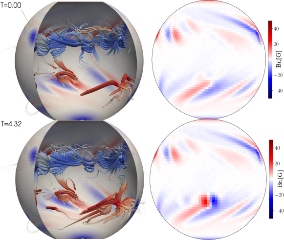
Figure 2: Formation of two magnetic regions in the South hemisphere during the growth phase of Cycle 23 in model S0. Left column shows the field lines of the non-axisymmetric magnetic field, and time is shown in days. Right column shows the surface radial magnetic field. The full animation of the magnetic field evolution is available online. The animation illustrates the formation of BMR in the South hemisphere. The BMR start as magnetic bubbles which eventually appear at the surface. Also, we see effect of the large-scale flow and the eddy magnetic diffusivity on evolution of the BMR’s remnants.

Figure 2 illustrates the formation of BMR simulated in model S0. The BMR start as magnetic bubbles which eventually appear at the surface. In addition, we see the corresponding poleward magnetic flux transport events that are formed from remnants of the BMR’s evolution due to the effects of differential rotation, meridional circulation, and magnetic eddy diffusivity.

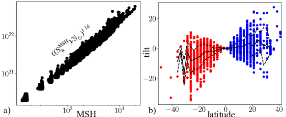
Figure 3: Model S0: a) Distribution of the BMR area and the magnetic flux, b) the BMR’s tilt. Blue color shows BMR from the northern hemisphere, and red color shows the southern hemisphere, the solid line shows the mean tilt, and the dashed lines show the tilt variance.

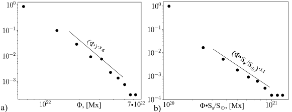
Figure 4: Model S0. a) Occurrence probability for the BMR flux magnitude, $\Phi$; b) the same for the BMR flux and area magnitude, $\Phi\cdot\mathrm{S_{a}}$

Next, we look at distributions of the BMR’s size, tilt angles and magnetic fluxes. We consider snapshots of the synoptic maps of the non-axisymmetric radial magnetic field and calculate the continuous area of the magnetic regions using the threshold of $10^{20}$ Mx in the pixel. We find the linear relation between the BMR’s area and flux, see Fig. 3a). This is in agreement with observational results (Nagovitsyn & Pevtsov, 2021). The distribution of the tilt angle shown in Fig. 3b is also in close agreement with observations (Nagovitsyn et al., 2021), including the nonlinear behavior at latitudes $>25^{\circ}$.

Figure 4 shows results for the probability distributions of the BMR’s flux magnitude, $\Phi$, and the power of the magnetic flux occupying the area $\mathrm{S_{a}}$, $\Phi\cdot\mathrm{S_{a}}$. These parameters show the power-law probability distributions, similarly to the observational analyses of Parnell et al. (2009), Muñoz-Jaramillo et al. (2015) and Nagovitsyn et al. (2021). However, the power-law indexes of in models are higher than in the observations, e.g., Parnell et al. (2009) found $P\propto\left(\Phi\cdot\mathrm{S_{a}}\right)^{-1.8}$. Our model reproduces the power law but with a steeper index $\approx-3.1$.

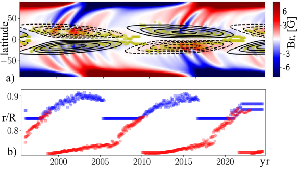
Figure 5: Model S0. a) Time-latitude diagram of the near surface toroidal magnetic field (contours in the range of $\pm 1$kG), surface radial magnetic field (color image), and positions of the BMR (squares) for model S0; b) the starting radial positions of the injected BMRs; blue squares mark the BMR injections from the upper part of the convection zone and the red squares mark the injections from the lower part.

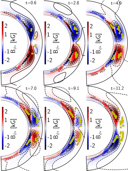
Figure 6: Snapshots of the axisymmetric magnetic field evolution during Cycle 23 in model S0. The BMR formation locations are marked by squares. To show the weak toroidal field near the equator, we use over-saturated color range. Vector-potential streamlines show the poloidal magnetic field, dashed lines reflect the anticlockwise direction of the field lines.

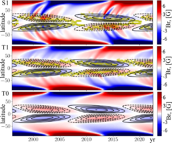
Figure 7: a) Time-latitude diagram of the near surface toroidal magnetic field (contours in range of $\pm 1$kG), surface radial magnetic field (color image), and positions of the BMR (squares) for model S1; b) and c) the same as a) for models T1 and T0.

3.2 The modeled magnetic field evolution

Figure 5 shows the time-latitude diagram of the surface radial magnetic field and the toroidal magnetic field in the subsurface shear layer for model S0. Also, we show the evolution of the BMR injection locations in radius. The butterfly diagrams are similar to the results of P22. The radial locations of the BMR injections mark the propagation of the dynamo wave from the bottom of the convection zone toward the surface (Kosovichev & Pipin, 2019; Pipin & Kosovichev, 2019). Figure 6 illustrates this propagation in a series of magnetic field meridional snapshots.

Noteworthy, the BMR injections from the bottom of the convection zone do not produce the surface BMR. This may be related to the restricted radial sizes of the BMR initiation sources (see Eq. 21). Nevertheless, as discussed later, such magnetic flux injections affect the surface non-axisymmetric magnetic field. With the described tuning of the $C_{\alpha}$ parameter, the BMR activity in model S0 satisfactorily fits the time-latitude variations of the near-surface toroidal magnetic field. Yet, near the equator, the BMR activity goes outside the modeled toroidal field evolution during the epoch of Cycle 23 minimum. The situation is clarified by Fig. 6. During the activity minima, the magnetic buoyancy mechanism initiates BMR not only from weak remnants of the toroidal magnetic field of the old cycle in the subsurface layers very near the equator but also from the deeper layers on the edge of the new dynamo wave of the next cycle.

Figure 7 shows the time-latitude diagrams for models S1, T0 and T1. Similarly to th e results of P22, we find that the model produces the smooth evolution of the surface radial magnetic field if we neglect the BMR’s tilt. The comparison of models S0 and T1 shows that details of the magnetic buoyancy mechanism and latitudinal locations of the BMR activity are important for the magnetic cycle parameters (Mackay & Yeates, 2012; Miesch & Dikpati, 2014). For comparison, we show the results for the pure axisymmetric model, T0, as well. For the given $C_{\alpha}$, model T0 has the activity cycle (half of the full dynamo period) of about 10.5 years, which is shorter than the periods of models T1 and S0, which include the BMR activity.

Figure 8 shows the mean absolute magnitude of the surface radial magnetic field, $\overline{\left|\mathbf{B}_{r}\right|}$, and the ratio of the mean magnitude of the axisymmetric surface field, ${\left|\overline{\mathbf{B}}_{r}\right|}$ to $\overline{\left|\mathbf{B}_{r}\right|}$. This ratio characterizes the level of the non-axisymmetry of the surface activity in our models. To compare with observations, we use the synoptic maps of the radial magnetic field from the KPO, SOLIS and SDO/HMI data archives (Harvey et al., 1980; Bertello et al., 2014; Scherrer et al., 2012). Using the synoptic maps, we calculate the surface mean of the unsigned radial magnetic field and the same for the axisymmetric radial magnetic field. We find that, in the observations, the value of $\overline{\left|\mathbf{B}_{r}\right|}$ reaches about 20-25 G at the solar maxima, and it was around 15 G in Solar Cycles 23 and 24. Bearing in mind the large-scale character of the magnetic activity in our model, we also compare our results with $\overline{\left|\mathbf{B}_{r}\right|}$ calculated f or non-axisymmetric spherical harmonics of the angular order $m<11$. We find a satisfactory agreement of models S0 and S2 with the solar observations. Model S0 shows that Solar Cycle 25, started in 2019, can be the same or a little higher than Cycle 24. The same is likely true in model S2.

However, the basal level of $\overline{\left|\mathbf{B}_{r}\right|}$ during the solar minima is about by a factor of 2 smaller than in the solar observations. This is reflected in the behavior of the non-axisymmetry parameter ${\left|\overline{\mathbf{B}}_{r}\right|}/\overline{\left|\mathbf{B}_{r}\right|}$, as well. It seems that our model misses some parts of the dynamo process that are essential for the large-scale non-axisymmetric magnetic field of the Sun. Interestingly, the contribution of the BMR activity to the axisymmetric magnetic field increases to the observational level just after the magnetic cycle maximum (see the dashed red curve in Fig. 8a). Model S2 shows the same behavior.

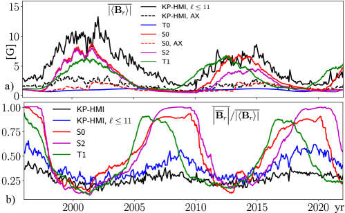
Figure 8: a) The mean absolute magnitude of the surface radial magnetic field; b) the ratio of the mean absolute magnitude of the axisymmetric surface field component to the mean magnitude of the surface radial magnetic field, $\overline{\left|\overline{\mathbf{B}}_{r}\right|}/\overline{\left|\left\langle\mathbf{B}_{r}\right\rangle\right|}$.

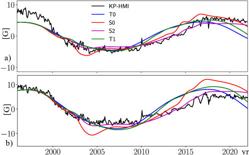
Figure 9: a) The mean axisymmetric radial magnetic field above $60^{\circ}$ latitude at the surface; b) the same above $70^{\circ}$ latitude.

Figure 9 shows the evolution of the polar magnetic field calculated by averaging the North-South anti-symmetric radial field components for latitudes higher than $60$ and $70$ degrees. We see that the polar field in the solar observations shows only a little change between these two measurements during the epoch of solar minimum around 1996. At the same time, the dynamo model shows significant changes in the latitude range in the polar field definition. Model T0 without BMR shows the same magnitude of the polar field for the cycle minima in 1996, 2007, and 2018. Model T1, with random initialization of BMR, shows a slight increase of the polar magnetic field during the minima due to the BMR contribution to the polar field magnitude. The same effect is found for model S0; although the magnitude of the mean-field $\alpha$-effect in this model was decreased in Cycles 23 and 24 to match the observed properties of Cycle 24. The mean latitude of the BMR injections in the data-driven model S0 (NOAA data driven model) is lower than in model T1 with the random BMR initialization. Model S2 shows the best fit for the solar data reproducing plateaus during the minima of Solar Cycles 23 and 24.

In our simulations, we investigated various possibilities to reproduce the basic parameters of Solar Cycles 23 and 24. Besides the long-term variations of the mean-field parameter $C_{\alpha}$, we considered $\alpha_{\beta}$ variations. In such cases, to bring the model in the best agreement with observations, we needed to assume very small values $C_{\beta}$ (corresponding to the mean BMR tilt) during the declining phase of Cycle 23 and the growth phase of Cycle 24. However, the observational results of Tlatov et al. (2013) do not show strong variations of the mean BMR tilt in different solar cycles. Yet, we can not exclude that Cycles 23 and 24 were affected by the emergence of the so-called “rogue” active regions (Nagy et al., 2017; Kumar et al., 2021). This point should be studied separately.

3.3 Torsional oscillations and meridional circulation variations

We find the BMR activity makes a substantial contribution in variation of the zonal flow and meridional circulation at the surface. The Fig10 show the surface time-latitude diagrams of the zonal acceleration, the Lorentz force from the BMRs and variations of the meridional circulation for the run S2.

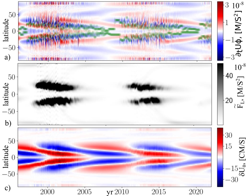
Figure 10: a) The background blue-red color show the surface variation of the zonal acceleration, the BMR activity latitude is shown by green squares; b) The time-latitude variations of the azimuthal force induced by the BMR activity; c) the time-latitude variations of the surface meridional circulation, the positive variation is toward the poles.

The Lorentz force induced by the BMR’s activity, $\tilde{F}_{L}$, is determined by the azimuthal average of the magnetic stress as follows:

$$\tilde{F}_{L} = \frac{1}{\overline{\rho}r\sin\theta}\boldsymbol{\nabla\cdot}\left(r\sin\theta\frac{\tilde{\mathbf{B}}\tilde{B}_{\phi}}{4\pi}\right).$$ (28)

Similar to results of Pipin & Kosovichev (2019), the model show the extended cycle of the torsional oscillation: the acceleration wave which started at about 50^∘ latitude around 1997 finished at equator after 20 years. The time-latitude pattern of the torsional oscillation results from a complicate force balance. The angular momentum balance includes, the dynamo induced variations of turbulent stresses, inertia forces, and variations of the meridional circulation, see a detailed study in the above cited paper. Noteworthy the amplitude of the forces which contribute the balance is more than order of magnitude higher than the magnitude of the zonal acceleration. Here, we see that the BMR activity produce the azimuthal acceleration of the near equatorial regions of the Sun.

The model shows the North-South asymmetry of the meridional circulation variations in the cycle 24. This asymmetry is accompanied by the trans-equatorial meridional flow of small magnitude during the growing phase of the cycle 24. Similar results was found recently by Getling et al. (2021) from helioseismology. In Fig10c we saturate the variations of high magnitude to show the weak variations of the meridional circulation in the polar regions. We see the decrease the meridional flow in the range of latitudes from 30^∘ to 50^∘ and from 60^∘ to 70^∘ during epochs of the magnetic activity maximum. The high latitude variations of the meridional circulation can affect the surface magnetic flux transport and evolution of the polar magnetic field.

4 Discussion and Conclusions

We model the physical parameters of Solar Cycles 23 and 24 using the nonlinear 3D mean-field dynamical dynamo model and the observational active region data. Our algorithm for the emergence of bipolar magnetic regions is based on the magnetic buoyancy effect acting on the unstable part of the large-scale magnetic field. The radial positions of the unstable regions are calculated using Parker’s magnetic instability condition. For the dynamo process distributed in the convection zone, this condition leads to the instability of the toroidal magnetic field at the front edge of the dynamo waves near the bottom of the convection zone and in its upper part, as illustrated in Fig. 6. For modeling the solar BMR injected from the upper part of the convection zone, we use the NOAA data base for coordinates and areas of active regions to specify the locations and sizes of the initial perturbations. For the unstable regions in the lower part of the convection zone, we use perturbations randomly distributed in time and longitude. Our results show that, in most cases, magnetic flux injections from the lower part of the convection zone do not result in the BMR formation on the surface. However, these injections affect the magnitude of the background non-axisymmetric magnetic field on the surface. Our dynamo models show the basal level of the non-axisymmetric magnetic field during the solar minima is about a factor of two smaller than in the solar observations. The possible reason is that our BMR algorithm is not sufficient for deep initialization sources. This affects the onset and decay of the large-scale non-axisymmetric magnetic activity.

The BMR distributions generated by our dynamo models show that the magnetic flux is directly proportional to BMR’s areas. This result is equally applied to the data-driven models S0, S1, and S2, and models T1 and T2 with the random distribution of the BMR sizes and longitudinal initialization points. The same proportionality was found in observations by Nagovitsyn & Pevtsov (2021) for the sunspot groups areas. The distribution of the BMR vs. the magnetic flux and area shows the inverse power-law of index -3.1. This qualitatively agrees with the results of Parnell et al. (2009), Muñoz-Jaramillo et al. (2015), and Nagovitsyn et al. (2021). However, they found a less steep power law for the large-scale part of the magnetic field distributions.

In our models, the BMR’s tilt is given theoretically, and it is directly related to the near-surface $\alpha$-effect Stix, 1974; Pipin, 2022. The latitudinal profile of the tilt follows the $\cos\theta$ dependence, where $\theta$ is co-latitude. We choose the BMR’s tilt to be randomly fluctuating about the mean. The resulting tilt distribution agrees with the solar observations (e.g. Nagovitsyn et al., 2021). Also, these authors found a tendency for the nonlinear behavior of tilt at latitudes $>25^{\circ}$. Our model shows similar behavior. It is caused by the $\alpha$-effect modulation due to the large-scale toroidal magnetic field.

In general, the dynamo solution of our model follows the Parker-Yoshimura law (Pipin 2021). In the weakly nonlinear regime the dynamo period of the Parker-Yoshimura dynamo waves is linearly connected with the $\alpha$ effect magnitude (Noyes et al. 1984). Naturally, the distributed dynamo models demonstrate the Waldmeier rules, as well (Pipin & Kosovichev 2011b). We exploited these properties to model the prolonged cycle 23 using the temporal decrease of the turbulent $\alpha$-effect. Generally, we can not exclude the other reasons for unusual behavior of cycle 23. In particular, Dikpati et al. (2010), using the flux-transport model, argued that the long cycle 23 can be due to increase of the meridional circulation cell. They suggested that in the standard situation the solar dynamo is controlled by two meridional circulation cell per hemisphere , and the “polar” cell has the inverted circulation in compare to the main “equatorial” cell. For the strongly nonlinear case the model can reproduce the multiple cell circulation pattern. Results of Pipin (2021) showed that this can happen on the fast rotating solar analogs. The dynamo period in this case is about 2 year. This is substantially less than the solar cycle period. It is an open question whether the model can reproduce the multiple cell in latitude for the nonmagnetic case. Pipin & Kosovichev (2019) found that for the solar-type dynamo the model shows a decrease of the surface poleward flow at high latitude during the magnetic activity maxima. Similar results are suggested by the helioseismology analysis of Getling et al. (2021). Here, we demonstrated this effect in the modelled cycles 23 and 24. Simultaneously, we find that the hemispheric asymmetry of the sunspot activity during the growing phase of cycle 24 results in the North-South asymmetry of the meridional circulation variations. This asymmetry is accompanied by the trans-equatorial meridional flow of small magnitude during that epoch. The variations of the meridional circulation are closely related with the torsional oscillations. These variations show the North-South asymmetry during the modelled cycle 24, as well. The model shows that the BMR activity induced the azimuthal acceleration force toward equator. It has the same order of magnitude as the other sources of the torsional oscillations due to the large-scale dynamo induced variations of turbulent stresses, inertia forces, and variations of the meridional circulation, (see, Pipin & Kosovichev, 2019).

Similar to Obridko et al. (2021) and Pipin (2022), we conclude that our initial modeling of Solar Cycles 22 and 23, which includes a combination of the global mean-field dynamo and emerging bipolar magnetic regions (BMR), shows that the BMR activity plays a significant role by affecting the strength and duration of the solar cycles. It was missing in the previous Parker-type dynamo models of the solar cycle. However, the data-driven models show that the BMR effect alone cannot explain the weak Cycle 24. The decrease in the cycle amplitude and the prolonged preceding minimum were probably caused by a decrease of the turbulent helicity in the bulk of the convection zone during the decaying phase of Cycle 23.

Acknowledgments

VP and VT thank the financial support of the Ministry of Science and Higher Education of the Russian Federation (Subsidy No.075-GZ/C3569/278). AK thanks the partial support of NASA grants: NNX14AB70G, 80NSSC20K0602, 80NSSC20K1320, and 80NSSC22M0162.

Data Availability Statements. The data underlying this article are available by request.

References

- Babcock (1961) Babcock, H. W. 1961, ApJ, 133, 572, doi: 10.1086/147060
- Bertello et al. (2014) Bertello, L., Pevtsov, A. A., Petrie, G. J. D., & Keys, D. 2014, Sol. Phys., 289, 2419, doi: 10.1007/s11207-014-0480-3
- Brandenburg (2005) Brandenburg, A. 2005, Astrophys. J., 625, 539
- Brandenburg (2018) Brandenburg, A. 2018, Journal of Plasma Physics, 84, 735840404, doi: 10.1017/S0022377818000806
- Brandenburg & Subramanian (2005) Brandenburg, A., & Subramanian, K. 2005, Phys. Rep., 417, 1, doi: 10.1016/j.physrep.2005.06.005
- Brun et al. (2014) Brun, A., Garcia, R., Houdek, G., Nandy, D., & Pinsonneault, M. 2014, Space Science Reviews, 1, doi: 10.1007/s11214-014-0117-8
- Charbonneau (2011) Charbonneau, P. 2011, Living Reviews in Solar Physics, 2, 2
- Dikpati (2016) Dikpati, M. 2016, Asian Journal of Physics, 25, 341. https://ui.adsabs.harvard.edu/abs/2016AsJPh..25..341D
- Dikpati et al. (2010) Dikpati, M., Gilman, P. A., de Toma, G., & Ulrich, R. K. 2010, Geophys. Res. Lett., 37, L14107, doi: 10.1029/2010GL044143
- Dikpati et al. (2016) Dikpati, M., Suresh, A., & Burkepile, J. 2016, Sol. Phys., 291, 339, doi: 10.1007/s11207-015-0831-8
- Getling et al. (2021) Getling, A. V., Kosovichev, A. G., & Zhao, J. 2021, ApJ, 908, L50, doi: 10.3847/2041-8213/abe45a
- Guerrero et al. (2016) Guerrero, G., Smolarkiewicz, P. K., de Gouveia Dal Pino, E. M., Kosovichev, A. G., & Mansour, N. N. 2016, ApJ, 828, L3, doi: 10.3847/2041-8205/828/1/L3
- Harris et al. (2020) Harris, C. R., Millman, K. J., van der Walt, S. J., et al. 2020, Nature, 585, 357, doi: 10.1038/s41586-020-2649-2
- Harvey et al. (1980) Harvey, J., Gillespie, B., Miedaner, P., & Slaughter, C. 1980, NASA STI/Recon Technical Report N, 81
- Hubbard & Brandenburg (2012) Hubbard, A., & Brandenburg, A. 2012, ApJ, 748, 51, doi: 10.1088/0004-637X/748/1/51
- Hunter (2007) Hunter, J. D. 2007, Computing in Science & Engineering, 9, 90, doi: 10.1109/MCSE.2007.55
- Kitchatinov (2004) Kitchatinov, L. L. 2004, Astronomy Reports, 48, 153, doi: 10.1134/1.1648079
- Kitchatinov & Nepomnyashchikh (2017) Kitchatinov, L. L., & Nepomnyashchikh, A. A. 2017, Astronomy Letters, 43, 332, doi: 10.1134/S106377371704003X
- Kitchatinov & Pipin (1993) Kitchatinov, L. L., & Pipin, V. V. 1993, A&A, 274, 647
- Kitchatinov et al. (1994) Kitchatinov, L. L., Pipin, V. V., & Ruediger, G. 1994, Astronomische Nachrichten, 315, 157
- Kitchatinov & Rüdiger (1992) Kitchatinov, L. L., & Rüdiger, G. 1992, A&A, 260, 494
- Kitchatinov & Rudiger (1993) Kitchatinov, L. L., & Rudiger, G. 1993, A&A, 276, 96
- Kitchatinov & Rüdiger (2005) Kitchatinov, L. L., & Rüdiger, G. 2005, Astronomische Nachrichten, 326, 379, doi: 10.1002/asna.200510368
- Kleeorin & Rogachevskii (1999) Kleeorin, N., & Rogachevskii, I. 1999, Phys. Rev.E, 59, 6724
- Kosovichev & Pipin (2019) Kosovichev, A. G., & Pipin, V. V. 2019, ApJ, 871, L20, doi: 10.3847/2041-8213/aafe82
- Krause & Rädler (1980) Krause, F., & Rädler, K.-H. 1980, Mean-Field Magnetohydrodynamics and Dynamo Theory (Berlin: Akademie-Verlag), 271
- Kumar et al. (2021) Kumar, P., Nagy, M., Lemerle, A., Karak, B. B., & Petrovay, K. 2021, ApJ, 909, 87, doi: 10.3847/1538-4357/abdbb4
- Leighton (1969) Leighton, R. B. 1969, ApJ, 156, 1, doi: 10.1086/149943
- Mackay & Yeates (2012) Mackay, D. H., & Yeates, A. R. 2012, Living Reviews in Solar Physics, 9, 6, doi: 10.12942/lrsp-2012-6
- Miesch & Dikpati (2014) Miesch, M. S., & Dikpati, M. 2014, ApJ, 785, L8, doi: 10.1088/2041-8205/785/1/L8
- Mitra et al. (2010) Mitra, D., Candelaresi, S., Chatterjee, P., Tavakol, R., & Brandenburg, A. 2010, Astronomische Nachrichten, 331, 130, doi: 10.1002/asna.200911308
- Moffatt (1978) Moffatt, H. K. 1978, Magnetic Field Generation in Electrically Conducting Fluids (Cambridge, England: Cambridge University Press)
- Muñoz-Jaramillo et al. (2015) Muñoz-Jaramillo, A., Senkpeil, R. R., Windmueller, J. C., et al. 2015, ApJ, 800, 48, doi: 10.1088/0004-637X/800/1/48
- Nagovitsyn et al. (2021) Nagovitsyn, Y. A., Osipova, A. A., & Pevtsov, A. A. 2021, MNRAS, 501, 2782, doi: 10.1093/mnras/staa3848
- Nagovitsyn & Pevtsov (2021) Nagovitsyn, Y. A., & Pevtsov, A. A. 2021, ApJ, 906, 27, doi: 10.3847/1538-4357/abc82d
- Nagy et al. (2017) Nagy, M., Lemerle, A., Labonville, F., Petrovay, K., & Charbonneau, P. 2017, Sol. Phys., 292, 167, doi: 10.1007/s11207-017-1194-0
- Noyes et al. (1984) Noyes, R. W., Weiss, N. O., & Vaughan, A. H. 1984, ApJ, 287, 769, doi: 10.1086/162735
- Obridko et al. (2021) Obridko, V. N., Pipin, V. V., Sokoloff, D., & Shibalova, A. S. 2021, MNRAS, 504, 4990, doi: 10.1093/mnras/stab1062
- Parker (1955) Parker, E. 1955, Astrophys. J., 122, 293
- Parker (1955) Parker, E. N. 1955, ApJ, 121, 491, doi: 10.1086/146010
- Parker (1971) —. 1971, ApJ, 163, 279, doi: 10.1086/150766
- Parker (1979) Parker, E. N. 1979, Cosmical magnetic fields: Their origin and their activity (Oxford: Clarendon Press)
- Parnell et al. (2009) Parnell, C. E., DeForest, C. E., Hagenaar, H. J., et al. 2009, ApJ, 698, 75, doi: 10.1088/0004-637X/698/1/75
- Paxton et al. (2011) Paxton, B., Bildsten, L., Dotter, A., et al. 2011, ApJS, 192, 3, doi: 10.1088/0067-0049/192/1/3
- Paxton et al. (2013) Paxton, B., Cantiello, M., Arras, P., et al. 2013, ApJS, 208, 4, doi: 10.1088/0067-0049/208/1/4
- Pipin (2008) Pipin, V. V. 2008, Geophysical and Astrophysical Fluid Dynamics, 102, 21
- Pipin (2018) —. 2018, Journal of Atmospheric and Solar-Terrestrial Physics, 179, 185, doi: 10.1016/j.jastp.2018.07.010
- Pipin (2021) —. 2021, MNRAS, 502, 2565, doi: 10.1093/mnras/stab033
- Pipin (2022) —. 2022, MNRAS, 514, 1522, doi: 10.1093/mnras/stac1434
- Pipin & Kitchatinov (2000) Pipin, V. V., & Kitchatinov, L. L. 2000, Astronomy Reports, 44, 771, doi: 10.1134/1.1320504
- Pipin & Kosovichev (2011a) Pipin, V. V., & Kosovichev, A. G. 2011a, ApJL, 727, L45, doi: 10.1088/2041-8205/727/2/L45
- Pipin & Kosovichev (2011b) —. 2011b, ApJ, 741, 1, doi: 10.1088/0004-637X/741/1/1
- Pipin & Kosovichev (2015) Pipin, V. V., & Kosovichev, A. G. 2015, The Astrophysical Journal, 813, 134. http://stacks.iop.org/0004-637X/813/i=2/a=134
- Pipin & Kosovichev (2018) Pipin, V. V., & Kosovichev, A. G. 2018, ApJ, 854, 67, doi: 10.3847/1538-4357/aaa759
- Pipin & Kosovichev (2019) —. 2019, ApJ, 887, 215, doi: 10.3847/1538-4357/ab5952
- Pipin & Kosovichev (2020) —. 2020, ApJ, 900, 26, doi: 10.3847/1538-4357/aba4ad
- Pipin et al. (2013) Pipin, V. V., Sokoloff, D. D., Zhang, H., & Kuzanyan, K. M. 2013, ApJ, 768, 46, doi: 10.1088/0004-637X/768/1/46
- Raedler (1980) Raedler, K.-H. 1980, Astronomische Nachrichten, 301, 101
- Rempel (2005) Rempel, M. 2005, ApJ, 631, 1286, doi: 10.1086/432610
- Roberts & Soward (1975) Roberts, P., & Soward, A. 1975, Astron. Nachr., 296, 49
- Ruediger & Brandenburg (1995) Ruediger, G., & Brandenburg, A. 1995, A&A, 296, 557
- Schaeffer (2013) Schaeffer, N. 2013, Geochemistry, Geophysics, Geosystems, 14, 751, doi: 10.1002/ggge.20071
- Scherrer et al. (2012) Scherrer, P. H., Schou, J., Bush, R. I., et al. 2012, Sol. Phys., 275, 207, doi: 10.1007/s11207-011-9834-2
- Schrinner (2011) Schrinner, M. 2011, A&A, 533, A108, doi: 10.1051/0004-6361/201116642
- Schrinner et al. (2011) Schrinner, M., Petitdemange, L., & Dormy, E. 2011, A&A, 530, A140, doi: 10.1051/0004-6361/201016372
- Shukurov & Subramanian (2021) Shukurov, A., & Subramanian, K. 2021, Astrophysical Magnetic Fields: From Galaxies to the Early Universe, Cambridge Astrophysics (Cambridge University Press), doi: 10.1017/9781139046657
- Stix (1974) Stix, M. 1974, A&A, 37, 121. https://ui.adsabs.harvard.edu/abs/1974A&A....37..121S
- Sullivan & Kaszynski (2019) Sullivan, C. B., & Kaszynski, A. 2019, Journal of Open Source Software, 4, 1450, doi: 10.21105/joss.01450
- Tlatov et al. (2013) Tlatov, A., Illarionov, E., Sokoloff, D., & Pipin, V. 2013, MNRAS, 432, 2975, doi: 10.1093/mnras/stt659
- Vidotto et al. (2018) Vidotto, A. A., Lehmann, L. T., Jardine, M., & Pevtsov, A. A. 2018, MNRAS, 480, 477, doi: 10.1093/mnras/sty1926
- Virtanen et al. (2020) Virtanen, P., Gommers, R., Oliphant, T. E., et al. 2020, Nature Methods, 17, 261, doi: 10.1038/s41592-019-0686-2
- Warnecke et al. (2014) Warnecke, J., Käpylä, P. J., Käpylä, M. J., & Brandenburg, A. 2014, ApJ, 796, L12, doi: 10.1088/2041-8205/796/1/L12
- Warnecke et al. (2018) Warnecke, J., Rheinhardt, M., Tuomisto, S., et al. 2018, A&A, 609, A51, doi: 10.1051/0004-6361/201628136
- Warnecke et al. (2021) Warnecke, J., Rheinhardt, M., Viviani, M., et al. 2021, ApJ, 919, L13, doi: 10.3847/2041-8213/ac1db5
- Yoshimura (1975) Yoshimura, H. 1975, ApJ, 201, 740, doi: 10.1086/153940