Systematic Evaluation of Predictive Fairness

Abstract

Mitigating bias in training on biased datasets is an important open problem. Several techniques have been proposed, however the typical evaluation regime is very limited, considering very narrow data conditions. For instance, the effect of target class imbalance and stereotyping is under-studied. To address this gap, we examine the performance of various debiasing methods across multiple tasks, spanning binary classification (Twitter sentiment), multi-class classification (profession prediction), and regression (valence prediction). Through extensive experimentation, we find that data conditions have a strong influence on relative model performance, and that general conclusions cannot be drawn about method efficacy when evaluating only on standard datasets, as is current practice in fairness research. Our code is available at: https://github.com/HanXudong/Systematic_Evaluation_of_Predictive_Fairness.

1 Introduction and Background

Naively-trained models have been shown to encode and amplify biases in the training dataset, and exhibit performance disparities across author demographics (Hovy and Søgaard, 2015; Li et al., 2018; Wang et al., 2019). Various methods have been proposed to mitigate such biases, such as balanced training (Zhao et al., 2018; Han et al., 2022a), adversarial debiasing (Elazar and Goldberg, 2018; Han et al., 2021), and null-space projection (Ravfogel et al., 2020, 2022). However, experiments have largely been conducted on a handful of benchmark datasets such as Moji sentiment analysis (Blodgett et al., 2016) and Bios biography classification (De-Arteaga et al., 2019), under a narrow set of data conditions.

In this paper, we systematically explore the impact of data conditions on model accuracy and fairness, synthesising the following data conditions over real-world datasets: (1) target label (im)balance; (2) protected attribute (im)balance; (3) target label–protected attribute (im)balance (also known as “stereotyping”); and (4) target label arity. Consistent with the literature on fairness in NLP, we primarily focus on classification tasks, but also include preliminary text regression experiments. In doing so, we develop a novel framework for comprehensively evaluating the performance of debiasing methods under a range of data conditions, and use it to evaluate eight widely-used debiasing methods.

Our experimental results show that there is no single best model. Debiasing methods that account for both class disparities and demographic disparities are generally more robust, but are less effective in multi-class settings. For the regression task, our experiments indicate that existing debiasing approaches can substantially improve fairness, and that simple linear debiasing outperforms more complex methods.

2 Related Work

In this section, we first describe different fairness criteria, then examine work which has evaluated the effectiveness of debiasing methods from different perspectives.

Fairness Criteria

Studies in the fairness literature have proposed several definitions of fairness capturing different types of discrimination, such as group fairness Hardt et al. (2016); Zafar et al. (2017a); Cho et al. (2020); Zhao et al. (2020), individual fairness Sharifi-Malvajerdi et al. (2019); Yurochkin et al. (2020); Dwork et al. (2012), and causality-based fairness Wu et al. (2019); Zhang and Bareinboim (2018a, b). In this work, we focus on group fairness, where a model is considered to be fair if it performs identically across different demographic subgroups.

To quantify how predictions vary across different demographic subgroups, demographic parity Feldman et al. (2015); Zafar et al. (2017b); Cho et al. (2020), equal opportunity Hardt et al. (2016); Madras et al. (2018), and equalized odds Cho et al. (2020); Hardt et al. (2016); Madras et al. (2018) are widely-used notions. We present these in a setting where there are exactly two protected attribute labels (a “privileged” and “under-privileged” sub-population), consistent with how they are traditionally defined. Demographic parity ensures that models achieve the same positive prediction rate for the two demographic subgroups, not taking the ground-truth target label into consideration. Equal opportunity requires that models achieve the same true positive rate across the two subgroups for instances with a positive label. Equalized odds goes one step further in requiring that models achieve not only the same level of true positive rate but also the same level of false positive rate across the two groups.

Aligned with key applications such as loan approvals, most fairness metrics assume binary classification and focus on one label (e.g., loan approved.) When turning attention to a multi-class classification scenario, equal opportunity is a natural choice, as it can be easily reformulated by assigning the positive class to each candidate class under a 1-vs-rest formulation.

Effectiveness of Debiasing Methods

Beyond the standard definitions of fairness, a number of studies have examined the effectiveness of various debiasing methods in additional settings Gonen and Goldberg (2019); Meade et al. (2021); Lamba et al. (2021); Baldini et al. (2022); Chalkidis et al. (2022). For example, Meade et al. (2021) not only examine the effectiveness of various debiasing methods but also measure the impact of debiasing methods on a model’s language modeling ability and downstream task performance. Webster et al. (2020) find that existing pretrained models encode different degrees of gender correlations, despite their performance on target tasks being quite similar, motivating the need to consider different metrics when performing model selection. A similar effect is also observed by Baldini et al. (2022). Chalkidis et al. (2022) examine the effectiveness of debiasing methods over a multi-lingual benchmark dataset consisting of four subsets of legal documents, covering five languages and various sensitive attributes. They find that methods aiming to improve worse-case performance tend to fail in more realistic settings, where both target label and protected attribute distributions vary over time. Lamba et al. (2021) perform an empirical comparison of various debiasing methods in solving real-world problems in high-stakes settings, all of which take the form of binary classification tasks. However, the effectiveness of debiasing methods under different data distributions (in terms of target class and protected attribute) has not been systematically investigated.

3 Methods

Here we describe the methods employed to manipulate the dataset distributions for classification tasks, and then describe how we adopt debiasing methods to a regression setting.

3.1 Notation Preliminaries

Experiments are based on a dataset consisting of $n$ instances $\mathcal{D}=\{({\bm{x}}_{i},{\textnormal{y}}_{i},{\textnormal{z}}_{i})\}_{i=1}^{n}$, where ${\bm{x}}_{i}$ is an input vector, ${\textnormal{y}}_{i}\in\{{\textnormal{c}}\}_{{\textnormal{c}}=1}^{{\textnormal{C}}}$ represents target class label, and ${\textnormal{z}}_{i}\in\{{\textnormal{g}}\}_{{\textnormal{g}}=1}^{{\textnormal{G}}}$ is the group label, such as gender. $n_{{\textnormal{c}},{\textnormal{g}}}$ denotes the number of instances in a subset with target label c and protected label g, i.e., $\mathcal{D}_{{\textnormal{c}},{\textnormal{g}}}=\{({\bm{x}}_{i},{\textnormal{y}}_{i},{\textnormal{z}}_{i})|{\textnormal{y}}_{i}={\textnormal{c}},{\textnormal{z}}_{i}={\textnormal{g}}\}_{i=1}^{n}$. The corresponding empirical probability of combination of y and z values is $P({\textnormal{y}}={\textnormal{c}},{\textnormal{z}}={\textnormal{g}})=\frac{n_{{\textnormal{c}},{\textnormal{g}}}}{n}$.

3.2 Manipulating Label Distributions

To investigate the effectiveness of debiasing methods under different data distributions, we need the ability to create synthetic datasets $\mathcal{D}^{\prime}$ that follow arbitrary distributions $P^{\prime}({\textnormal{y}},{\textnormal{z}})$. Intuitively, given $m$ instances and the joint probability $P^{\prime}({\textnormal{y}}={\textnormal{c}},{\textnormal{z}}={\textnormal{g}})$, we can create each of the subsets $\mathcal{D}^{\prime}_{{\textnormal{c}},{\textnormal{g}}}$ by sampling $mP^{\prime}({\textnormal{y}}={\textnormal{c}},{\textnormal{z}}={\textnormal{g}})$ instances with replacement from $\mathcal{D}_{{\textnormal{c}},{\textnormal{g}}}$. However, each $P^{\prime}$ has ${\textnormal{C}}\times{\textnormal{G}}$ parameters, rendering a systematic analysis infeasible. Instead, we propose to control the joint distribution in an interpretable way, via a single parameter, and report results as graphs: Given a particular rate $0\leq\alpha\leq 1$, we define the arbitrary distribution $P^{\prime}({\textnormal{y}},{\textnormal{z}})$ as the interpolation between the empirical distribution $P({\textnormal{y}},{\textnormal{z}})$ and a distribution of interest $Q({\textnormal{y}},{\textnormal{z}})$:

$$P^{\prime}({\textnormal{y}},{\textnormal{z}})=(1-\alpha)P({\textnormal{y}},{\textnormal{z}})+\alpha Q({\textnormal{y}},{\textnormal{z}}).$$

Next, we adopt two balanced training objectives (Han et al., 2022a) as our $Q$ distributions, and discuss their relationship to fairness.

Conditional Balance (CB) follows the notion of equal opportunity and emphasises the balance of demographics within each class, i.e., $Q_{\text{CB}}({\textnormal{z}}={\textnormal{g}}|{\textnormal{y}}={\textnormal{c}})=\frac{1}{{\textnormal{G}}},\forall{\textnormal{g}}\in\{1,\dots,{\textnormal{G}}\},{\textnormal{y}}\in\{1,\dots,{\textnormal{C}}\}$. The resulting interpolation is:

$$P_{\text{CB}}^{\prime}({\textnormal{y}},{\textnormal{z}})=P({\textnormal{y}})[(1-\alpha)P({\textnormal{z}}|{\textnormal{y}})+\alpha Q_{\text{CB}}({\textnormal{z}}|{\textnormal{y}})]$$

where the overall class distribution $P({\textnormal{y}})$ does not change with the value of $\alpha$.

Joint Balance (JB) goes one step further in taking both class balance and demographic balance into account, resulting in $Q_{\text{JB}}({\textnormal{z}}={\textnormal{g}},{\textnormal{y}}={\textnormal{c}})=\frac{1}{{\textnormal{C}}{\textnormal{G}}},\forall{\textnormal{g}}\in\{1,\dots,{\textnormal{G}}\},{\textnormal{y}}\in\{1,\dots,{\textnormal{C}}\}$. The interpolation

$$P_{\text{JB}}^{\prime}({\textnormal{y}},{\textnormal{z}})=(1-\alpha)P({\textnormal{y}},{\textnormal{z}})+\alpha Q_{\text{JB}}({\textnormal{y}},{\textnormal{z}})$$ (1)

ensures both class and demographic labels are more balanced with a larger $\alpha$.

Inverting the Bias $\alpha=0$ and $\alpha=1$ result in the original distribution and a balanced distribution, respectively. We extend the space of possible distributions, by also considering scenarios with $\alpha>1$, which result in “anti-stereotypical” distributions where majority classes and demographics are swapped to minorities.

Although the sum of adjusted probabilities is guaranteed to be $1$, it is possible to generate negative probabilities or values that are larger than $1$ after interpolation. In Appendix B, we describe the normalisation strategies to get a valid probability table. In this paper, we consider $\alpha\in[0,2]$ for our dataset interpolations. Taking the CB interpolation as an example, given $P(\mathrm{Female}|\mathrm{Nurse})=0.9$ (Section A.2), $\alpha=0,1,\mathrm{and}~{}2$ result in the adjusted $P^{\prime}(\mathrm{Female}|\mathrm{Nurse})=0.9,0.5,\mathrm{and}~{}0.1$, respectively. Consistent adjustments will be applied to other professions in the training dataset.

3.3 Debiasing for Regression Tasks

Regression models predict a real-valued target variable, rather than discrete values as in classification. Many existing fairness metrics and debiasing methods assume discrete target (and protected attribute) labels, and are thus not directly applicable to regression tasks, such as the equal opportunity criteria which measures disparities across demographics within each class (Roh et al., 2021; Shen et al., 2022).

As a first step towards applying debiasing methods to text regression tasks, we map the continuous target variables y into discrete values by approximating the real-valued outputs with quantile-based proxy labels $\tilde{{\textnormal{y}}}$. Specifically, let $\tilde{{\textnormal{y}}}$ denote the proxy label, such that the dataset for regression is $\mathcal{D}=\{({\bm{x}}_{i},{\textnormal{y}}_{i},{\textnormal{z}}_{i},\tilde{{\textnormal{y}}}_{i})\}_{i=1}^{n}$, where ${\textnormal{y}}\in\mathbb{R}$ is the continuous target label. Given a particular number of quantiles $\tilde{{\textnormal{C}}}$, y is converted into equal-sized buckets based on sample quantiles, resulting in categorical proxy labels $\tilde{{\textnormal{y}}}\in\{\tilde{{\textnormal{c}}}\}_{\tilde{{\textnormal{c}}}=1}^{\tilde{{\textnormal{C}}}}$. Two typical choices for $\tilde{{\textnormal{C}}}$ are 10 and 4, corresponding to deciles and quartiles, respectively.

In model training, we calculate losses based on real labels y, and identify protected groups based on $\tilde{{\textnormal{y}}}$. Appendix E presents further details for adopting debiasing methods to regression tasks.

4 Experiments

In this section we describe general settings across all experiments. In Appendix A, we provide full experimental details and dataset statistics.

4.1 Debiasing Methods

Our focus in this work is to examine the effectiveness of various debiasing methods on different dataset compositions and their applicability to regression tasks. As such, we take a representative sample of debiasing methods, populating the spectrum of pre-processing, in-processing, and post-processing approaches.

Vanilla:

The model is trained naively with cross-entropy loss, without taking bias mitigation into consideration (Vanilla).

Pre-processing:

perform downsampling or reweighting of the dataset before model training.

1. Downsampling (DS: Han et al. (2022a)): Bias mitigation is achieved by downsampling the dataset, by balancing it w.r.t. the protected attribute within each target class while preserving the original target class ratio.

2. Reweighting (RW: Han et al. (2022a)): Bias mitigation is achieved by assigning different weights to instances in the dataset, by reweighting based on the (inverse) of the joint distribution of the protected attribute and target classes.

In-processing:

perform adversarial training or directly optimise w.r.t. fairness criteria by either dynamically adjusting the sampling rate or penalising groups of instances.

1. Adversarial training (ADV: Elazar and Goldberg (2018); Li et al. (2018)) jointly trains a discriminator to predict the protected attribute, leading to representations agnostic to protected attributes.

2. Diverse adversarial training (DADV: Han et al. (2021)) trains multiple discriminators as above, with a pairwise orthogonality constraint over discriminators to encourage learning of different representational aspects.

3. Fair batch selection (FairBatch: Roh et al. (2021)) dynamically adjusts the instance resampling probability during training w.r.t. a given target class and protected attribute value, based on the equal opportunity criterion.

4. Equal opportunity (EO: Shen et al. (2022)) directly optimises for equal opportunity by penalising loss differences across protected groups via a regularisation term. We adopt two versions of optimising equal opportunity: enforcing equal opportunity by aligning group-wise losses within each class (EO_CLA), and enforcing equal opportunity globally by aligning class- and group wise loss with the overall model performance (EO_GLB).

Post-processing:

manipulate the learned representations to achieve fairness.

1. Iterative null-space projection (INLP: Ravfogel et al. (2020)) first learns dense representations with a cross-entropy loss, and then iteratively projects the representations to the null-space of discriminators for the protected attributes.

4.2 Evaluation Metrics

To evaluate model performance, we adopt Accuracy in our classification experiments, and Pearson correlation for the regression task.

To measure bias, following previous studies De-Arteaga et al. (2019); Ravfogel et al. (2020); Shen et al. (2022), we adopt root mean square of true positive rate gap over all classes (GAP), which is defined as $\text{GAP}=\sqrt{\frac{1}{{\textnormal{C}}}\sum_{{\textnormal{y}}}(\mathrm{GAP}^{\mathrm{TPR}}_{{\textnormal{y}}})^{2}}$. Here, $\mathrm{GAP}^{\mathrm{TPR}}_{{\textnormal{y}}}=|\mathrm{TPR}_{{\textnormal{y}},{\textnormal{z}}}-\mathrm{TPR}_{{\textnormal{y}},\neg{\textnormal{z}}}|,\forall{\textnormal{y}}$, and $\mathrm{TPR}_{{\textnormal{y}},{\textnormal{z}}}=\mathds{P}\{\hat{{\textnormal{y}}}={\textnormal{y}}|{\textnormal{y}},{\textnormal{z}}\}$, indicating the percentage of correct predictions among instances with the target class y and protected attribute label z. $\mathrm{GAP}^{\mathrm{TPR}}_{{\textnormal{y}}}$ measures the absolute performance difference between demographic subgroups conditioned on target label y, and a value of $0$ indicates that the model makes predictions independent of the protected attribute. To be consistent with our performance evaluation metrics (the higher the better), we define Fairness as $1-$GAP, where a value of 1 indicates there is no predictive bias.

4.3 Experimental Setup

For each dataset, we vary training set distributions while keeping the test set fixed. Document representations are first obtained from the given pretrained model without finetuning. Then document representations are fed into two feed-forward layers with a hidden size of 300, each followed by the $\tanh$ activation function. We use Adam Kingma and Ba (2014) to optimise the model for at most 100 epochs with early stopping, where training is stopped if no improvement is observed over the dev set for 5 epochs. All models are trained and evaluated on the same dataset splits, and models are selected based on their performance on the development set, as described in Section 4.4. All experiments are conducted with the fairlib library (Han et al., 2022c).

4.4 Model Selection

Simultaneously optimising models for performance and fairness is a multi-objective problem, making model selection a non-trivial task. In this work, following Han et al. (2022a), we perform model selection based on Distance to the Optimal point (DTO), where the optimal point represents the highest theoretical performance and fairness level any model can achieve. DTO supports the comparison of models by aggregating performance and fairness into a single figure of merit, where lower is better.

5 Binary Classification

The task is to predict the binary sentiment (happy and sad) of a given English tweet, as determined by the (redacted) emoji used in the tweet. Each tweet is also associated with a binary protected attribute, reflecting the ethnicity of the tweet author, as captured in the register of the English: Standard American English (SAE) and African American English (AAE).

We use the widely-used Twitter emoji dataset Blodgett et al. (2016); Ravfogel et al. (2020); Shen et al. (2022), denoted as Moji. The training dataset is balanced in terms of both sentiment and ethnicity in general, but skewed in terms of sentiment–ethnicity combinations, $P(AAE|\textsc{happy})=P(SAE|\textsc{sad})=0.8$. Due to the fact the the original dataset has been balanced with respect to targets and demographics, the CB interpolation is exactly the same as the JB interpolation (Section 3.2).

For ease of comparison with previous work (Subramanian et al., 2021b), we refer to the CB interpolation as varying “stereotyping” ($P^{\prime}({\textnormal{z}}|{\textnormal{y}})$) with balanced target class distribution. To explore the effects of target class distribution and stereotyping, we further experiment in various controlled settings: (1) varying class ratio ($P^{\prime}({\textnormal{y}})$) without stereotyping ($P^{\prime}({\textnormal{z}}|{\textnormal{y}})=0.5$); (2) varying stereotyping with imbalanced target class distribution; and (3) varying class ratio with stereotyping. Finally, we summarise our findings with respect to the effectiveness and robustness of various debiasing methods over different class-stereotyping compositions.

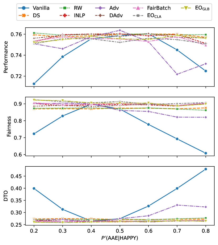
Figure 1: Results for Moji when varying $P^{\prime}(AAE|\textsc{happy})$ with $P^{\prime}(\textsc{happy})=P^{\prime}(\textsc{sad})$.

5.1 Varying Stereotyping with Balanced Class Distribution (CB Interpolation)

Here, both sentiment and ethnicity are balanced, but skewed in terms of $P^{\prime}(AAE|\textsc{happy})$ and $P^{\prime}(SAE|\textsc{sad})$, ranging from 0.2 to 0.8. For example, when the ratio of AAE is 0.2, the training data composition is 10% happy–AAE, 40% happy–SAE, 40% sad–AAE, and 10% sad–SAE.

Figure 1 shows model performance in terms of Accuracy, Fairness, and DTO. All models except for Vanilla and INLP perform similarly over varying degrees of stereotyping across metrics, indicating that most models are robust to different degrees of stereotyping using the proposed model selection approach. Turning to Vanilla, we find that Accuracy, Fairness, and DTO all vary greatly as we increase the degree of stereotyping, indicating that stereotyping affects naively-trained models in terms of both performance and fairness.

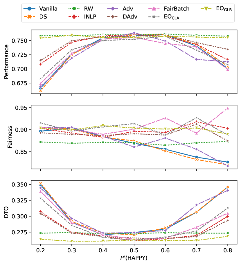
Figure 2: Results for Moji when varying $P^{\prime}(\textsc{happy})$ with $P^{\prime}(AAE|\textsc{happy})=P^{\prime}(SAE|\textsc{sad})=0.5$.

5.2 Varying Class Ratio with no Stereotyping

In this setting, $P^{\prime}(AAE|{\textnormal{y}})=P^{\prime}(SAE|{\textnormal{y}}),\forall{\textnormal{y}}$, and we vary $P({\textnormal{y}}=\textsc{happy})$ from 0.2 to 0.8. For example, when the ratio of happy is 0.2, the training dataset contains 10% happy–AAE, 10% happy–SAE, 40% sad–AAE, and 40% sad–SAE.

From Figure 2, we can see that most models are sensitive to the target class distribution, especially in terms of Accuracy and DTO. RW and EO_GLB are exceptions, and are clearly superior methods when the dataset is free of stereotyping, no matter the target class distribution. The Fairness achieved by all models in this setting does not vary greatly (ranging from approximately $0.82$ to $0.90$), indicating that target class distributions with no stereotyping have limited effect in biasing naively-trained models.

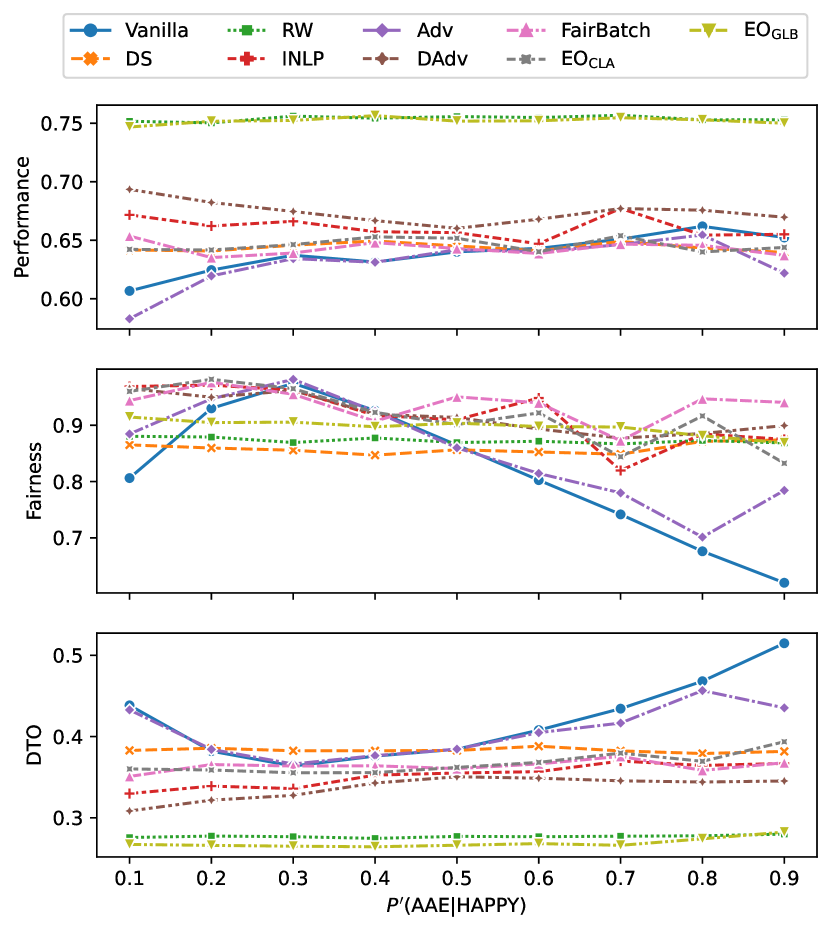
Figure 3: Results of varying $P^{\prime}(AAE|\textsc{happy})$ with $P^{\prime}(\textsc{happy})=0.9$.

5.3 Varying Stereotyping with Imbalanced Class Distributions

In this setting, the target class distribution is imbalanced, in that $P^{\prime}(\textsc{happy})=0.9$ in the training dataset. $P^{\prime}(AAE|\textsc{happy})$ and $P^{\prime}(SAE|\textsc{sad})$ varies from 0.1 to 0.9. For example, when the ratio of AAE is 0.2, the training dataset contains 18% happy–AAE, 72% happy–SAE, 8% sad–AAE, and 2% sad–SAE, respectively.

From Figure 3, we can see that RW and EO_GLB consistently achieve the best performance in terms of Accuracy and DTO. Fairness for DS, RW, and EO_GLB is robust to varying degrees of AAE stereotyping, while the remaining methods are sensitive to stereotyping.

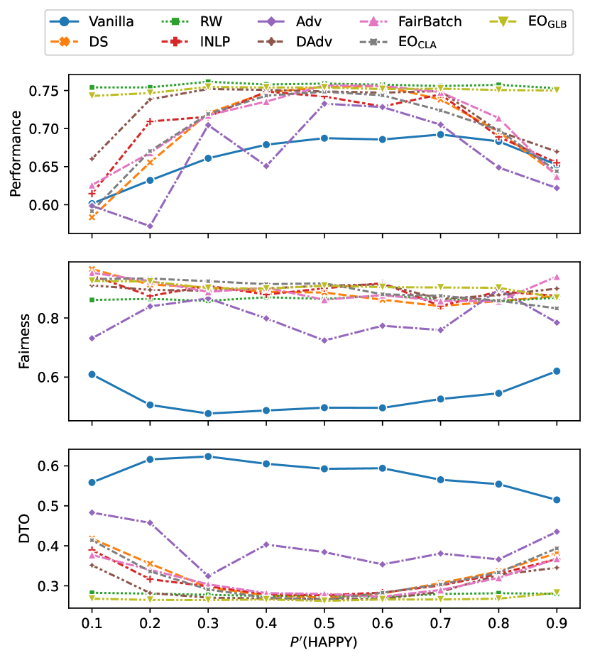
Figure 4: Results for Moji when varying $P^{\prime}(\textsc{happy})$ with $P^{\prime}(AAE|\textsc{happy})=P^{\prime}(SAE|\textsc{sad})=0.9$.

5.4 Varying Class Ratio with Stereotyping

In this setting, the ethnicity distribution is imbalanced, in that $P^{\prime}(AAE|\textsc{happy})=P^{\prime}(SAE|\textsc{sad})=90\%$. $P^{\prime}(\textsc{happy})$ varies from 0.1 to 0.9. For example, when the ratio of happy is 0.2, the training dataset consists of 18% happy–AAE, 2% happy–SAE, 8% sad–AAE, and 72% sad–SAE, respectively.

From Figure 4, we can see that both RW and EO_GLB consistently achieve the best performance in terms of Accuracy and DTO, while the remaining methods are quite sensitive to the target class distribution in terms of Accuracy and DTO, and all models except for Vanilla and INLP achieve relatively consistent Fairness.

5.5 Summary

In this section, we have performed various experiments on the Twitter sentiment analysis task with varying dataset composition. Looking at results from Sections 5.1 and 5.3, we can see that all models except for Vanilla and INLP are quite consistent with respect to Accuracy, Fairness, and DTO, with RW and EO_GLB consistently achieving competitive performance in terms of Accuracy, Fairness, and DTO. Comparing results from Sections 5.2 and 5.4, the performance of all models except for RW and EO_GLB vary with respect to the target class distribution in terms of Accuracy and DTO, while all models perform consistently in terms of Fairness.

6 Multi-class Classification

We next turn to our second dataset, which is a multi-class classification task with natural imbalance in both target labels and protected groups.

The dataset consists of online biographies, labeled with one of 28 occupations (target labels) and binary author gender (protected label), and the task is to predict the occupation from the biography text (Bios, De-Arteaga et al. (2019)).

6.1 Results

Figures 5 and 6 present results for JB and CB interpolation over Bios. As introduced in Section 3.2, JB jointly adjusts the extent of stereotyping and target class imbalance, and CB focuses on the stereotyping.

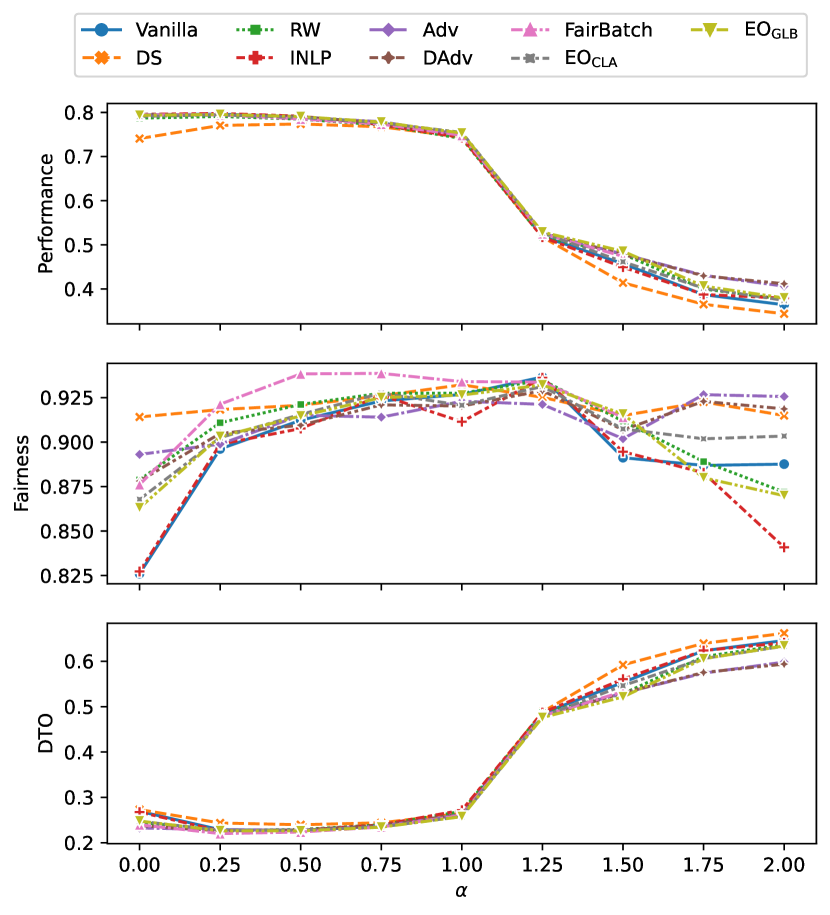
Figure 5: Results for Bios when varying the interpolation ratio under JB. Target classes and demographics are jointly balanced at $\alpha=1$.

JB Interpolation:

As the value of $\alpha$ increases from 0 to 1, the training distribution becomes more balanced for both class and protected attributes, resulting in fairness improvements. As the performance is measured as the overall accuracy, which is essentially a micro-average and oblivious to class balance, the overall performance does not improve with a more balanced class distribution.

With the $\alpha$ value further increasing from 1 to 2, both class and protected attribute distributions are biased in the opposite direction, i.e., majority groups become minority groups. As a result, the fairness for Vanilla decreases substantially. Recall that the test dataset distribution is unchanged throughout the experiments (and has an identical distribution to the $\alpha=0$ setting), leading to large drops in performance of models trained on anti-biased class distributions.

Consistent with Sections 5.3 and 5.4, EO_GLB outperforms other debiasing methods when the class and protected attributes are both imbalanced, as it explicitly mitigates both biases simultaneously.

We notice that FairBatch relies on a large number of instances per class/group combination for effective resampling, and as a result is highly vulnerable to input data bias, which can be seen in the fact that there are no results for FairBatch in imbalanced settings ($\alpha=1.75$ and $2$).

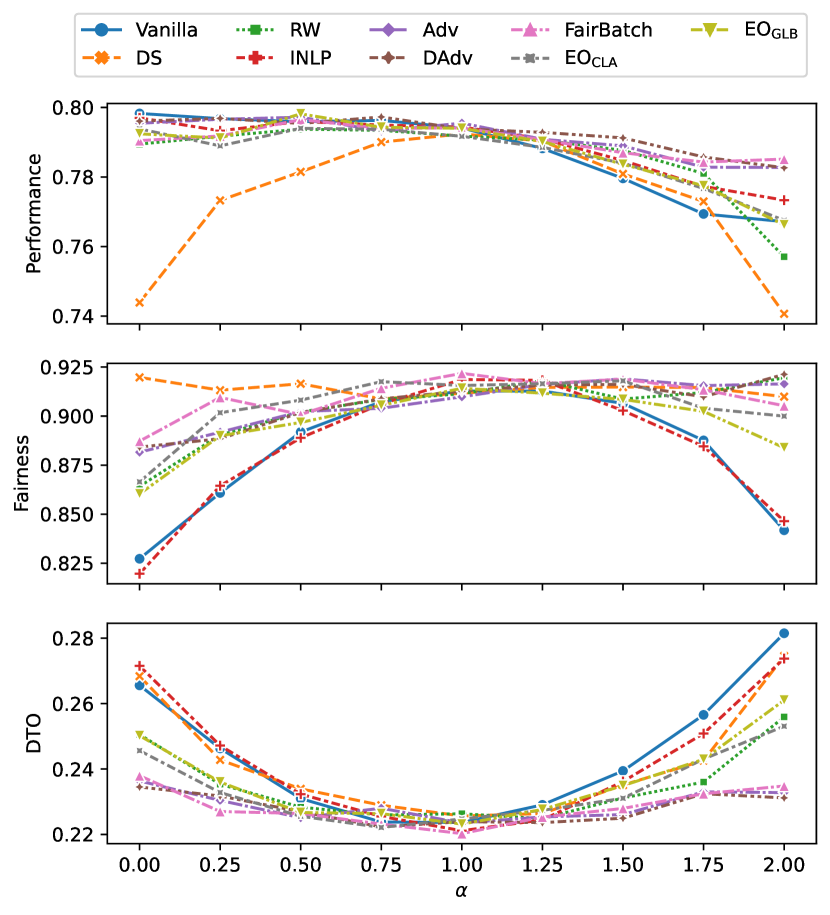
Figure 6: Results for Bios when varying the interpolation ratio under CB. Stereotyping ratios are balanced for the the $\alpha=0$ setting.

CB Interpolation:

When focusing on stereotyping, different methods achieve similar performance except for DS, due to the simple sampling strategy substantially reducing the training dataset size.

In terms of Fairness, debasing approaches except for INLP are robust to different stereotyping levels. EO_GLB achieves worse performance than EO_CLA because it additionally considers class imbalance. As ADV and DADV mitigate biases without taking the class into account, their debiasing results are not affected by the number of classes and perform best for this data set.

7 Regression

We finally turn to the regression setting. The task is to predict the valence (sentiment) of a given Facebook post, where each post is assigned a valence score by two trained annotators in the range 1–9 and the task is to predict the average of the two scores Preoţiuc-Pietro et al. (2016). Additionally, each post is associated with a binary authorship gender label. In our experiments, results are reported based on 5-fold cross-validation.

7.1 Results

Instead of measuring fairness with GAP based on TPR scores for classification tasks, we focus on the Pearson correlation disparities across demographic groups. From Table 1 we can see that all models improve over Vanilla. Overall, INLP is the best debiasing method, which we hypothesise is because its linear structure is more appropriate for the small data set, while the deeper methods appear to overfit.

Models	Pearson $\uparrow$	Fairness $\uparrow$	DTO $\downarrow$
Vanilla	63.38$\pm$2.48	85.18$\pm$0.40	39.50
RW	63.69$\pm$1.50	84.73$\pm$0.91	39.39
INLP	70.46$\pm$0.00	88.54$\pm$0.00	31.68
ADV	69.41$\pm$0.39	85.81$\pm$0.33	33.72
DADV	69.02$\pm$0.85	85.66$\pm$0.63	34.14
FairBatch	68.25$\pm$1.47	85.18$\pm$0.62	35.04
EOCLA	65.88$\pm$0.89	85.05$\pm$0.40	37.25
EOGLB	65.37$\pm$1.29	85.03$\pm$0.39	37.73

Table 1: Experimental results on the Valence test set.

8 General Discussion and Recommendations

So far, we have shown that there is no single best model across different data conditions, and data conditions should be a key consideration in fairness evaluation. In this section, we divide debiasing methods into three families, and summarize their robustness to skewed training data distributions.

Balancing demographics in the training dataset

DS and RW are representatives of this family, and are simple and effective. In addition, such methods are flexible as the training dataset is pre-processed before model training, and any candidate models on the original dataset can be applied to the debiased dataset.

However, DS methods are sensitive to group sizes. Considering an extreme setting where the smallest subset in the training dataset has 0 instances, i.e., $\mathcal{D}_{{\textnormal{c}},{\textnormal{g}}}=\emptyset$, DS will result in an empty training set. For instance, the group size distribution is highly skewed for the regression task, and DS resulted in $r=0$ Pearson correlation (Table 4 in Appendix). Similar problems are associated with up-sampling methods, which can increase the training set size dramatically.

In addition, when considering multiple protected attributes, such as intersectional groups and gerrymandering groups (Subramanian et al., 2021a), the number of groups increases exponentially with the number of protected attributes to be considered. As a result, the joint distributions can be highly skewed, and these two families of methods (resampling and reweighting) may not be appropriate choices.

Lastly, skewed protected label distributions in the training dataset is not the only source of bias (Wang et al., 2019). For example, as shown in Figure 1 the Vanilla model trained over balanced versions ($P^{\prime}(AAE|\textsc{happy})=0.5$) of the Moji dataset is less fair than the Vanilla model trained over a biased dataset where $P^{\prime}(AAE|\textsc{happy})=0.4$.

Learning fair hidden representations

ADV, DADV, and INLP represent a family of methods that learn fair representations through unlearning discriminators. Since the training and unlearning of discriminators do not take into account target class information, these methods are robust to the number of classes and naturally generalize to regression tasks.

However, these methods are not capable of modelling conditional independence for the equal opportunity criterion without taking target class into consideration, resulting in worse DTO than other debiasing methods over Moji (Section 5). To achieve equal opportunity fairness, different discriminators can be trained for each target class to capture conditional independence (Ravfogel et al., 2020; Han et al., 2022b). But training target-specific discriminators assumes target labels to be discrete, which is sensitive to the number of classes.

Another limitation of this family of methods is associated with the discriminator learning: the discriminator can also suffer from long-tail learning problems, i.e. skewed demographics, and lead to biased estimations of protected information. The unlearning of biased discriminators limits the method’s contribution to bias mitigation, which can be seen from Figures 3 and 4 in Section 5.

Minimising loss disparities across demographic groups

FairBatch, EO_CLA, and EO_GLB provide a practical approximation of expected fairness in using empirical risk-based objectives, and directly optimize for empirical risk parity during training.

Similar to balanced training approaches, resampling and reweighting are also used in mitigating loss disparities, where FairBatch adjusts resampling probabilities for batch selection, and EO_CLA and EO_GLB assign instances different weights depending on the demographic group they belong to. However, minimising loss disparities can be more flexible than balanced training – for example, instance weights are dynamically adjusted by EO_CLA and EO_GLB, and can take on negative values to aggressively reduce a bias towards favouring of over-represented groups.

Conversely, drawbacks associated with resampling and reweighting also apply to this family. For example, FairBatch indeed broke down (an error raised) when $\mathcal{D}_{{\textnormal{c}},{\textnormal{g}}}=\emptyset$ for the minority group in a particular minibatch for a Bios dataset variant where the smallest group size is close to 0 (Section 6).

Minimising loss difference is also less efficient in multi-class settings, as it adjusts weights based on class information during training, making optimisation harder.

9 Conclusion

In this work, we presented a novel framework for investigating different classification dataset distributions with a single parameter, and used it to systematically examine the effectiveness of debiasing methods in binary classification and multi-classification settings based on real-world datasets. We also presented preliminary analysis of debiasing methods in a regression setting, including proposing a method for adapting existing debiasing methods to regression tasks. Based on extensive experimentation over three datasets, we found that there was no single best model. Debiasing methods that account for both class and demographic disparities are generally more robust, but are less efficient at achieving fairness in multi-class settings. For the regression task, we demonstrated that existing debiasing approaches can substantially improve fairness, and that the simple linear debiasing method outperforms more complex techniques. In summary, there is no universal best debiasing method across all tasks, and data conditions have a large impact on different models. As such, we propose that future research adopts our evaluation framework as a means of more comprehensively evaluating debiasing methods.

Limitations

This paper focuses on fairness evaluation w.r.t. equal opportunity fairness. While a more comprehensive study should include a diversity of fairness objectives, we note that previous work (Han et al., 2021) has shown that evaluation results w.r.t. different fairness criteria are highly correlated.

Consistent with previous work, we restrict our experiments to categorical protected attributes (binary gender, ethnicity) acknowledging that other relevant attributes (such as age) are more naturally modeled as a continuous variable. Since the aim of this paper is a systematic evaluation of existing debiasing methods, which were all developed specifically for categorical protected attributes, the extension to continuous variables is beyond the scope of this paper. A simple adaptation to continuous demographic labels like age is discretization, which we leave as a promising direction for future work.

For similar reasons, we use established data sets as provided by the original authors and used in relevant prior work, and acknowledge the simplified treatment of gender as a binary variable which reflects neither the diversity nor the fluidity of the underlying concept Dev et al. (2021).

Ethical Consideration

In this work, we focus on examining the effectiveness of various debiasing methods on both classification and regression tasks, where the protected attribute is either ethnicity or gender. However, their effectiveness in reducing bias towards other protected attributes is not necessarily guaranteed. Furthermore, the protected attributes examined in our work are limited to binary labels, whose effectiveness in debiasing $N$-ary protected attributes are left to future work.

Appendix A Datasets and Implementation Details

A.1 Moji

Following previous studies Ravfogel et al. (2020); Han et al. (2021), the original training dataset is balanced with respect to both sentiment and ethnicity but skewed in terms of sentiment–ethnicity combinations (40% happy-AAE, 10% happy-SAE, 10% sad-AAE, and 40% sad-SAE, respectively). Note that the dev and test set are balanced in terms of sentiment–ethnicity combinations. The dataset contains 100K/8K/8K train/dev/test instances.

When varying training set distributions, we keep the 8k test instances unchanged.

We use DeepMoji Felbo et al. (2017) to obtain Twitter representations, where DeepMoji is a model pretrained over 1.2 billion English tweets and DeepMoji is fixed during model training. For all models, the learning rate is 3e-3, and the batch size is 1,024. Hyperparameter tuning for each model is described in Section C.1.

Profession	Total	Male	Female	Ratio
dietitian	2567	183	2384	0.929
nurse	12316	1127	11189	0.908
paralegal	1146	173	973	0.849
yoga_teacher	1076	166	910	0.846
model	4867	840	4027	0.827
interior_designer	949	182	767	0.808
psychologist	11945	4530	7415	0.621
teacher	10531	4188	6343	0.602
journalist	12960	6545	6415	0.495
physician	26648	13492	13156	0.494
poet	4558	2323	2235	0.490
painter	5025	2727	2298	0.457
personal_trainer	928	505	423	0.456
professor	76748	42130	34618	0.451
attorney	21169	13064	8105	0.383
accountant	3660	2317	1343	0.367
photographer	15773	10141	5632	0.357
dentist	9479	6133	3346	0.353
filmmaker	4545	3048	1497	0.329
chiropractor	1725	1271	454	0.263
pastor	1638	1245	393	0.240
architect	6568	5014	1554	0.237
comedian	1824	1439	385	0.211
composer	3637	3042	595	0.164
software_engineer	4492	3783	709	0.158
surgeon	8829	7521	1308	0.148
dj	964	828	136	0.141
rapper	911	823	88	0.097

Table 2: Statistics of the Bios training dataset. Ratio stands for the percentage of female individuals for each profession

A.2 Bios

We denote the data set as Bios, and use the same split as prior work Ravfogel et al. (2020); Shen et al. (2022) of 257k train, 40k dev and 99k test instances. Table 2 shows the number of instances of each profession, the number of male and female individuals of each profession, and the ratio of female individuals for each profession in the Bios training dataset. As the target label distribution is highly skewed, we adjust the distribution over Bios dataset with 30K training instances, such that each profession contains about 1K instances, which is similar to the size of the smallest target group.

We use the “CLS” token representation of the pretrained uncased BERT-base Devlin et al. (2019) to obtain text representations, where BERT-base is fixed during model training, aligning with previous studies Ravfogel et al. (2020); Shen et al. (2022). Hyperparameter settings for all models are available in Section D.1.

A.3 Valence

The dataset contains 2,883 posts, of which male and female authors account for $51\%$ and $49\%$ respectively.

We use the “CLS” token representation of the pretrained uncased BERT-base Devlin et al. (2019) to obtain post representations, where BERT-base is fixed during model training. Hyperparameter settings are described in Section F.1.

For this task, we use Pearson, mean absolute error (MAE), and root mean square error (RMSE) to evaluate model performance; and we use the Pearson difference (Pearson-GAP), MAE difference (MAE-GAP), and RMSE difference (RMSE-GAP) between male and female groups to evaluate model bias.

Appendix B Normalization For Probability Table

To make sure the resulting probability table $P^{\prime}$ is valid, we normalize the table by replacing negative values with 0, and normalize the sum to 1. Specifically, let $S=\sum_{\textnormal{y}}\sum_{\textnormal{z}}P^{\prime}({\textnormal{y}},{\textnormal{z}})$ denote the sum of probabilities. The normalization is $P^{\prime}({\textnormal{y}},{\textnormal{z}})=\frac{P^{\prime}({\textnormal{y}},{\textnormal{z}})}{S},\forall{\textnormal{y}},{\textnormal{z}}$.

Appendix C Twitter Sentiment Analysis

C.1 Hyperparameters

For all models except for Vanilla, DS, and RW, where no extra hyperparameters are introduced, we tune the most sensitive hyperparameters through grid search. For INLP, following Ravfogel et al. (2020), we use $300$ linear SVM classifiers. For ADV, we tune $\lambda_{\text{adv}}$ from 1e-3 to 1e3 with 60 trials. For DADV, we further tune $\lambda_{\text{diverse}}$ within the range of 1e-1 and 1e5 with 60 trials. For FairBatch, we tune $\alpha$ from 1e-3 to 1e1 with 40 trials. For EO_CLA and EO_GLB, we tune $\lambda$ within the range of 1e-3 and 1e1 with 40 trials, respectively. All hyperparameters are finetuned on the Moji dev set.

C.2 Results

Models	Accuracy $\uparrow$	Fairness $\uparrow$	DTO $\downarrow$
Vanilla	72.49$\pm$0.18	60.79$\pm$1.12	47.90
DS	75.92$\pm$0.32	86.88$\pm$1.08	27.43
RW	75.96$\pm$0.28	86.18$\pm$0.97	27.73
INLP	73.18$\pm$0.00	82.04$\pm$0.00	32.28
ADV	75.12$\pm$0.83	90.40$\pm$1.75	26.67
DADV	75.65$\pm$0.12	89.94$\pm$0.50	26.34
FairBatch	74.96$\pm$0.41	90.49$\pm$0.49	26.79
EOCLA	75.09$\pm$0.25	90.70$\pm$0.87	26.59
EOGLB	75.60$\pm$0.17	89.83$\pm$0.60	26.43

Table 3: Experimental results on the Moji test set (averaged over 5 runs); Bold $=$ Best Performance; $\uparrow=$ the higher the better; $\downarrow=$ the lower the better.

Table 3 shows the results achieved by various methods. All debiasing methods can reduce bias significantly while improving model performance in terms of Accuracy.

Appendix D Profession Classification

D.1 Hyperparameters

For all models, the learning rate is 3e-3, and the batch size is 1,024. For all models we tune the most sensitive hyperparameters through grid search except for Vanilla, DS, and RW as there is no extra hyperparameters introduced for these three methods. For INLP, following Ravfogel et al. (2020), we use $300$ linear SVM classifiers. For ADV, we tune $\lambda_{\text{adv}}$ from 1e-3 to 1e3 with 60 trials. For DADV, we further tune $\lambda_{\text{diverse}}$ within the range of 1e-1 and 1e5 with 60 trials. For FairBatch, we tune $\alpha$ from 1e-3 to 1e1 with 40 trials. For EO_CLA and EO_GLB, we tune $\lambda$ within the range of 1e-3 and 1e1 with 40 trials, respectively. All hyperparameters are finetuned on the Bios dev set.

Appendix E Adaptation For Regression Tasks

E.1 EO_CLA (Shen et al., 2022)

The debiasing objective for classification tasks is to minimise cross-entropy loss disparities across different protected groups within each class, $\mathcal{L}_{\text{eo}}^{\text{class}}=\lambda\sum_{{\textnormal{c}}=1}^{{\textnormal{C}}}\sum_{{\textnormal{g}}=1}^{{\textnormal{G}}}|\mathcal{L}^{{\textnormal{c}},{\textnormal{g}}}_{ce}-\mathcal{L}_{ce}^{{\textnormal{c}}}|$, where $\mathcal{L}^{{\textnormal{c}},{\textnormal{g}}}_{ce}$ and $\mathcal{L}_{ce}^{{\textnormal{y}}}$ are the cross-entropy losses for subset of instances $\{({\bm{x}}_{i},{\textnormal{y}}_{i},{\textnormal{z}}_{i})|{\textnormal{y}}_{i}={\textnormal{c}},{\textnormal{z}}_{i}={\textnormal{g}}\}_{i=1}^{n}$ and $\{({\bm{x}}_{i},{\textnormal{y}}_{i},{\textnormal{z}}_{i})|{\textnormal{y}}_{i}={\textnormal{c}}\}_{i=1}^{n}$, respectively.

Clearly, the identification of subsets requires categorical labels, which is based on proxy labels for regression tasks. By replace the cross-entropy loss with mean squared error loss ($\mathcal{L}_{mse}$), the objective for EO_CLA is $\mathcal{L}_{\text{eo}}^{\text{reg}}=\lambda\sum_{\tilde{{\textnormal{c}}}=1}^{\tilde{{\textnormal{C}}}}\sum_{{\textnormal{g}}=1}^{{\textnormal{G}}}|\mathcal{L}^{\tilde{{\textnormal{c}}},{\textnormal{g}}}_{mse}-\mathcal{L}_{mse}^{\tilde{{\textnormal{c}}}}|$ where $\mathcal{L}^{\tilde{{\textnormal{c}}},{\textnormal{g}}}_{mse}$ and $\mathcal{L}_{mse}^{\tilde{{\textnormal{c}}}}$ are the cross-entropy losses for subset of instances $\{({\bm{x}}_{i},{\textnormal{y}}_{i},{\textnormal{z}}_{i},\tilde{{\textnormal{y}}}_{i})|\tilde{{\textnormal{y}}}_{i}=\tilde{{\textnormal{c}}},{\textnormal{z}}_{i}={\textnormal{g}}\}_{i=1}^{n}$ and $\{({\bm{x}}_{i},{\textnormal{y}}_{i},{\textnormal{z}}_{i},\tilde{{\textnormal{y}}}_{i})|\tilde{{\textnormal{y}}}_{i}=\tilde{{\textnormal{c}}}\}_{i=1}^{n}$, respectively.

Models	Pearson $\uparrow$	Pearson-GAP $\downarrow$	MAE $\downarrow$	MAE-GAP $\downarrow$	RMSE $\downarrow$	RMSE-GAP $\downarrow$
Vanilla	0.63$\pm$0.04	0.06$\pm$0.05	0.78$\pm$0.03	0.08$\pm$0.01	1.00$\pm$0.04	0.09$\pm$0.02
DS	0.00$\pm$0.04	0.08$\pm$0.04	0.97$\pm$0.05	0.06$\pm$0.03	1.23$\pm$0.05	0.05$\pm$0.03
RW	0.62$\pm$0.03	0.06$\pm$0.05	0.78$\pm$0.02	0.08$\pm$0.02	0.99$\pm$0.03	0.09$\pm$0.04
INLP	0.66$\pm$0.04	0.09$\pm$0.04	0.71$\pm$0.04	0.03$\pm$0.02	0.92$\pm$0.04	0.04$\pm$0.02
ADV	0.67$\pm$0.03	0.06$\pm$0.06	0.72$\pm$0.03	0.06$\pm$0.04	0.93$\pm$0.04	0.09$\pm$0.06
DADV	0.67$\pm$0.03	0.07$\pm$0.06	0.72$\pm$0.02	0.06$\pm$0.02	0.92$\pm$0.02	0.07$\pm$0.05
FairBatch	0.67$\pm$0.03	0.06$\pm$0.06	0.71$\pm$0.01	0.06$\pm$0.02	0.92$\pm$0.02	0.07$\pm$0.04
EOCLA	0.65$\pm$0.03	0.07$\pm$0.05	0.75$\pm$0.03	0.07$\pm$0.01	0.96$\pm$0.03	0.08$\pm$0.02
EOGLB	0.64$\pm$0.03	0.06$\pm$0.06	0.76$\pm$0.03	0.08$\pm$0.02	0.97$\pm$0.04	0.10$\pm$0.04

Table 4: Experimental results on the Facebook post dataset with respect to arousal; the best performance is indicated in bold.

Appendix F Arousal Prediction of Facebook Posts

F.1 Hyperparameters

For all models, the learning rate is 7e-4, the batch size is 64, the number of hidden layers is 1, and hidden layer size is 200. Each model is trained with mean squared loss with a weight decay of 1e-3. For all models except for Vanilla, we need to bin instances, as the dataset is small and the range of valence scores is large; otherwise, these methods cannot be applied in their original form. In this work, instances are grouped into 4 bins. For all models we tune the most sensitive hyperparameters through grid search except for Vanilla, DS, and RW as there are no extra hyperparameters introduced for these three methods. For INLP, following Ravfogel et al. (2020), we use $200$ linear regressors. For ADV, we tune $\lambda_{\text{adv}}$ from 1e-3 to 1e3 with 60 trials. For DADV, we further tune $\lambda_{\text{diverse}}$ within the range of 1e-1 to 1e5 with 60 trials. For FairBatch, we tune $\alpha$ from 1e-3 to 1e1 with 40 trials. For EO_CLA and EO_GLB, we tune $\lambda$ within the range of 1e-3 to 1e1 with 40 trials, respectively. All hyperparameters are finetuned on the dev set.

F.2 Results

Table 4 presents the results on the arousal dataset.

References

- Baldini et al. (2022) Ioana Baldini, Dennis Wei, Karthikeyan Natesan Ramamurthy, Moninder Singh, and Mikhail Yurochkin. 2022. Your fairness may vary: Pretrained language model fairness in toxic text classification. In Findings of the Association for Computational Linguistics, pages 2245–2262.
- Blodgett et al. (2016) Su Lin Blodgett, Lisa Green, and Brendan O’Connor. 2016. Demographic dialectal variation in social media: A case study of African-American English. In Proceedings of the 2016 Conference on Empirical Methods in Natural Language Processing, pages 1119–1130.
- Chalkidis et al. (2022) Ilias Chalkidis, Tommaso Pasini, Sheng Zhang, Letizia Tomada, Sebastian Schwemer, and Anders Søgaard. 2022. FairLex: A multilingual benchmark for evaluating fairness in legal text processing. In Proceedings of the 60th Annual Meeting of the Association for Computational Linguistics (Volume 1: Long Papers), pages 4389–4406.
- Cho et al. (2020) Jaewoong Cho, Gyeongjo Hwang, and Changho Suh. 2020. A fair classifier using kernel density estimation. In Advances in Neural Information Processing Systems.
- De-Arteaga et al. (2019) Maria De-Arteaga, Alexey Romanov, Hanna Wallach, Jennifer Chayes, Christian Borgs, Alexandra Chouldechova, Sahin Geyik, Krishnaram Kenthapadi, and Adam Tauman Kalai. 2019. Bias in bios: A case study of semantic representation bias in a high-stakes setting. In Proceedings of the Conference on Fairness, Accountability, and Transparency, pages 120–128.
- Dev et al. (2021) Sunipa Dev, Masoud Monajatipoor, Anaelia Ovalle, Arjun Subramonian, Jeff Phillips, and Kai-Wei Chang. 2021. Harms of gender exclusivity and challenges in non-binary representation in language technologies. In Proceedings of the 2021 Conference on Empirical Methods in Natural Language Processing, pages 1968–1994, Online and Punta Cana, Dominican Republic. Association for Computational Linguistics.
- Devlin et al. (2019) Jacob Devlin, Ming-Wei Chang, Kenton Lee, and Kristina Toutanova. 2019. BERT: Pre-training of deep bidirectional transformers for language understanding. In Proceedings of the 2019 Conference of the North American Chapter of the Association for Computational Linguistics: Human Language Technologies, Volume 1 (Long and Short Papers), pages 4171–4186.
- Dwork et al. (2012) Cynthia Dwork, Moritz Hardt, Toniann Pitassi, Omer Reingold, and Richard S. Zemel. 2012. Fairness through awareness. In Innovations in Theoretical Computer Science 2012, pages 214–226.
- Elazar and Goldberg (2018) Yanai Elazar and Yoav Goldberg. 2018. Adversarial removal of demographic attributes from text data. In Proceedings of the 2018 Conference on Empirical Methods in Natural Language Processing, pages 11–21.
- Felbo et al. (2017) Bjarke Felbo, Alan Mislove, Anders Søgaard, Iyad Rahwan, and Sune Lehmann. 2017. Using millions of emoji occurrences to learn any-domain representations for detecting sentiment, emotion and sarcasm. In Proceedings of the 2017 Conference on Empirical Methods in Natural Language Processing, pages 1615–1625.
- Feldman et al. (2015) Michael Feldman, Sorelle A. Friedler, John Moeller, Carlos Scheidegger, and Suresh Venkatasubramanian. 2015. Certifying and removing disparate impact. In Proceedings of the 21th ACM SIGKDD International Conference on Knowledge Discovery and Data Mining, pages 259–268.
- Gonen and Goldberg (2019) Hila Gonen and Yoav Goldberg. 2019. Lipstick on a pig: Debiasing methods cover up systematic gender biases in word embeddings but do not remove them. In Proceedings of the 2019 Conference of the North American Chapter of the Association for Computational Linguistics: Human Language Technologies, pages 609–614.
- Han et al. (2021) Xudong Han, Timothy Baldwin, and Trevor Cohn. 2021. Diverse adversaries for mitigating bias in training. In Proceedings of the 16th Conference of the European Chapter of the Association for Computational Linguistics: Main Volume, pages 2760–2765.
- Han et al. (2022a) Xudong Han, Timothy Baldwin, and Trevor Cohn. 2022a. Balancing out bias: Achieving fairness through training reweighting. In Proceedings of the 2022 Conference on Empirical Methods in Natural Language Processing (EMNLP 2022). To appear.
- Han et al. (2022b) Xudong Han, Timothy Baldwin, and Trevor Cohn. 2022b. Towards equal opportunity fairness through adversarial learning. ArXiv, abs/2203.06317.
- Han et al. (2022c) Xudong Han, Aili Shen, Yitong Li, Lea Frermann, Timothy Baldwin, and Trevor Cohn. 2022c. fairlib: A unified framework for assessing and improving classification fairness. In Proceedings of the 2022 Conference on Empirical Methods in Natural Language Processing (EMNLP 2022) Demo Session. To appear.
- Hardt et al. (2016) Moritz Hardt, Eric Price, and Nati Srebro. 2016. Equality of opportunity in supervised learning. In Advances in Neural Information Processing Systems, pages 3315–3323.
- Hovy and Søgaard (2015) Dirk Hovy and Anders Søgaard. 2015. Tagging performance correlates with author age. In Proceedings of the 53rd annual meeting of the Association for Computational Linguistics and the 7th International Joint Conference on Natural Language Processing (volume 2: Short papers), pages 483–488.
- Kingma and Ba (2014) Diederik P Kingma and Jimmy Ba. 2014. Adam: A method for stochastic optimization. arXiv preprint arXiv:1412.6980.
- Lamba et al. (2021) Hemank Lamba, Kit T Rodolfa, and Rayid Ghani. 2021. An empirical comparison of bias reduction methods on real-world problems in high-stakes policy settings. ACM SIGKDD Explorations Newsletter, 23(1):69–85.
- Li et al. (2018) Yitong Li, Timothy Baldwin, and Trevor Cohn. 2018. Towards robust and privacy-preserving text representations. In Proceedings of the 56th Annual Meeting of the Association for Computational Linguistics, pages 25–30.
- Madras et al. (2018) David Madras, Elliot Creager, Toniann Pitassi, and Richard S. Zemel. 2018. Learning adversarially fair and transferable representations. In Proceedings of the 35th International Conference on Machine Learning,, pages 3381–3390.
- Meade et al. (2021) Nicholas Meade, Elinor Poole-Dayan, and Siva Reddy. 2021. An empirical survey of the effectiveness of debiasing techniques for pre-trained language models. arXiv preprint arXiv:2110.08527.
- Preoţiuc-Pietro et al. (2016) Daniel Preoţiuc-Pietro, H Andrew Schwartz, Gregory Park, Johannes Eichstaedt, Margaret Kern, Lyle Ungar, and Elisabeth Shulman. 2016. Modelling valence and arousal in Facebook posts. In Proceedings of the 7th workshop on computational approaches to subjectivity, sentiment and social media analysis, pages 9–15.
- Ravfogel et al. (2020) Shauli Ravfogel, Yanai Elazar, Hila Gonen, Michael Twiton, and Yoav Goldberg. 2020. Null it out: Guarding protected attributes by iterative nullspace projection. In Proceedings of the 58th Annual Meeting of the Association for Computational Linguistics, pages 7237–7256.
- Ravfogel et al. (2022) Shauli Ravfogel, Michael Twiton, Yoav Goldberg, and Ryan Cotterell. 2022. Linear adversarial concept erasure. arXiv preprint arXiv:2201.12091.
- Roh et al. (2021) Yuji Roh, Kangwook Lee, Steven Euijong Whang, and Changho Suh. 2021. Fairbatch: Batch selection for model fairness. In Proceedings of the 9th International Conference on Learning Representations.
- Sharifi-Malvajerdi et al. (2019) Saeed Sharifi-Malvajerdi, Michael J. Kearns, and Aaron Roth. 2019. Average individual fairness: Algorithms, generalization and experiments. In Advances in Neural Information Processing Systems, pages 8240–8249.
- Shen et al. (2022) Aili Shen, Xudong Han, Trevor Cohn, Timothy Baldwin, and Lea Frermann. 2022. Optimising equal opportunity fairness in model training. CoRR, abs/2205.02393.
- Subramanian et al. (2021a) Shivashankar Subramanian, Xudong Han, Timothy Baldwin, Trevor Cohn, and Lea Frermann. 2021a. Evaluating debiasing techniques for intersectional biases. In Proceedings of the 2021 Conference on Empirical Methods in Natural Language Processing, pages 2492–2498.
- Subramanian et al. (2021b) Shivashankar Subramanian, Afshin Rahimi, Timothy Baldwin, Trevor Cohn, and Lea Frermann. 2021b. Fairness-aware class imbalanced learning. In Proceedings of the 2021 Conference on Empirical Methods in Natural Language Processing, pages 2045–2051.
- Wang et al. (2019) Tianlu Wang, Jieyu Zhao, Mark Yatskar, Kai-Wei Chang, and Vicente Ordonez. 2019. Balanced datasets are not enough: Estimating and mitigating gender bias in deep image representations. In Proceedings of the IEEE/CVF International Conference on Computer Vision, pages 5310–5319.
- Webster et al. (2020) Kellie Webster, Xuezhi Wang, Ian Tenney, Alex Beutel, Emily Pitler, Ellie Pavlick, Jilin Chen, and Slav Petrov. 2020. Measuring and reducing gendered correlations in pre-trained models. CoRR, abs/2010.06032.
- Wu et al. (2019) Yongkai Wu, Lu Zhang, and Xintao Wu. 2019. Counterfactual fairness: Unidentification, bound and algorithm. In Proceedings of the Twenty-Eighth International Joint Conference on Artificial Intelligence, pages 1438–1444.
- Yurochkin et al. (2020) Mikhail Yurochkin, Amanda Bower, and Yuekai Sun. 2020. Training individually fair ML models with sensitive subspace robustness. In Proceedings of the 8th International Conference on Learning Representations.
- Zafar et al. (2017a) Muhammad Bilal Zafar, Isabel Valera, Manuel Gomez-Rodriguez, and Krishna P. Gummadi. 2017a. Fairness beyond disparate treatment & disparate impact: Learning classification without disparate mistreatment. In Proceedings of the 26th International Conference on World Wide Web, pages 1171–1180.
- Zafar et al. (2017b) Muhammad Bilal Zafar, Isabel Valera, Manuel Gomez-Rodriguez, and Krishna P. Gummadi. 2017b. Fairness constraints: Mechanisms for fair classification. In Proceedings of the 20th International Conference on Artificial Intelligence and Statistics, volume 54, pages 962–970.
- Zhang and Bareinboim (2018a) Junzhe Zhang and Elias Bareinboim. 2018a. Equality of opportunity in classification: A causal approach. In Advances in Neural Information Processing Systems, pages 3675–3685.
- Zhang and Bareinboim (2018b) Junzhe Zhang and Elias Bareinboim. 2018b. Fairness in decision-making - the causal explanation formula. In Proceedings of the Thirty-Second AAAI Conference on Artificial Intelligence, pages 2037–2045.
- Zhao et al. (2020) Han Zhao, Amanda Coston, Tameem Adel, and Geoffrey J. Gordon. 2020. Conditional learning of fair representations. In Proceedings of the 8th International Conference on Learning Representations.
- Zhao et al. (2018) Jieyu Zhao, Tianlu Wang, Mark Yatskar, Vicente Ordonez, and Kai-Wei Chang. 2018. Gender bias in coreference resolution: Evaluation and debiasing methods. In Proceedings of the 2018 Conference of the North American Chapter of the Association for Computational Linguistics: Human Language Technologies, pages 15–20.