Combinatorial structures of the space of gradient vector fields on compact surfaces

Abstract.

A gradient flow is one of the fundamental objects from a theoretical and practical point of view. For instance, various phenomena are modeled as gradient flows. On the other hand, little is known about the topology of the space of gradient flows. For instance, it is not even known whether the space of gradient flows has non-simply-connected connected components. In this paper, to construct a foundation for describing the possible generic time evolution of gradient flows on surfaces with or without restriction conditions, we study the topology of the space of such flows under the non-existence of creations and annihilations of singular points. In fact, the space of gradient flows has non-contractible connected components.

1. Introduction

A gradient flow is one of the fundamental objects from a theoretical and practical point of view. In the time evolution of fluids on punctured spheres, some kinds of such fluids are modeled by gradient flows, and the topologies of streamlines can be changed by the creations and annihilations of singular points and physical boundaries. For instance, one can observe the creation of a physical boundary, which is a boundary of a stone on the surface of a river, when the water level of the river goes down as in Figure 1.

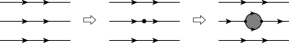
Figure 1. Creation of a physical boundary.

Notice that creations and annihilations of physical boundaries change the topologies of surfaces. On the other hand, the topologies of such fluids also can be changed by switching combinatorial structures of separatrices. Such combinatorial structures are studied from fluid mechanics [2, 7, 11], integrable systems [5], and dynamical systems [8, 14, 15, 16, 17, 22, 21, 20, 23].

From a dynamical system’s point of view, Smale [18] proved that any Morse flow (i.e. Morse-Smale flow without limit cycles) on a closed manifold is a gradient flow without separatrices from a saddle to a saddle. By a work of Andronov-Pontryagin [1] and a work of Peixoto [13], it is known that the set of Morse-Smale $C^{r}$-vector fields ($r\geq 1$) on a closed orientable surface $S$ is open dense in the space of $C^{r}$-vector fields on $S$ and that Morse-Smale $C^{r}$-vector fields are structurally stable in the space of vector fields. In particular, the set of $C^{r}$-Morse vector fields (i.e Morse-Smale vector fields without limit cycles) on a closed orientable surface is open dense in the space of gradient vector fields. By these facts, one characterizes a “generic” non-Morse gradient flow on a compact surface to describe a generic time evaluation of gradient flows on orientable compact surfaces (e.g. solutions of differential equations) which is an alternating sequence of Morse flows and instantaneous non-Morse gradient flows under no physical or symmetric restrictions [6]. On the other hand, “non-generic” intermediate vector fields (e.g. fluids with symmetric vortex pairs) naturally appear under physical or symmetric restrictions. For instance, degenerate saddle connections are the reasons for “non-genericity”. Though the hierarchical structure of the space of gradient flows is one of the foundations for describing generic time evaluations, only the low codimensional structures were studied. More globally, we ask the following question.

Question 1.

Does the space of topological equivalence classes of gradient vector fields on a manifold have non-contractible connected components, under the non-existence of creations and annihilations of singular points?

In this paper, we demonstrate that there is such a non-contractible connected component of the space of topological equivalence classes of gradient vector fields on a manifold.

The present paper consists of seven sections. In the next section, as preliminaries, we introduce fundamental concepts. In §3, we study the combinatorial structure of the space of gradient flows under the non-existence of creations and annihilations of singular points and boundary components. In §4, the abstract cell complex structure and filtration of the space of gradient flows are described. In §5, we demonstrate the non-contractibility of a connected component of the space of gradient flows. In §6, we describe the combinatorial structure of the space of Morse-Smale-like flows. In the final section, we state a future work and an open question.

2. Preliminaries

2.1. Notion of dynamical systems

A flow is a continuous $\mathbb{R}$-action on a paracompact manifold. Let $v:\mathbb{R}\times M\to M$ be a flow on a paracompact manifold $M$. For $t\in\mathbb{R}$, define $v_{t}:M\to S$ by $v_{t}:=v(t,\cdot)$. For a point $x$ of $M$, we denote by $O(x)$ the orbit of $x$ (i.e. $O(x):=\{v_{t}(x)\mid t\in\mathbb{R}\}=v(\mathbb{R},x)$). A positive (resp. negative) orbit of $x$ is $v(\mathbb{R}_{>0},x)$ (resp. $v(\mathbb{R}_{<0},x)$), denoted by $O^{+}(x)$ (resp. $O^{-}(x)$). A point $x$ of $M$ is singular if $x=v_{t}(x)$ for any $t\in\mathbb{R}$ and is periodic if there is a positive number $T>0$ such that $x=v_{T}(x)$ and $x\neq v_{t}(x)$ for any $t\in(0,T)$. A point is closed if it is singular or periodic. An orbit is singular (resp. periodic, closed) if it contains singular (resp. periodic, closed) points. Denote by $\mathop{\mathrm{Sing}}(v)$ (resp. $\mathop{\mathrm{Per}}(v)$, $\mathop{\mathrm{Cl}}(v)$) the set of singular (resp. periodic, closed) points. Denote by $\overline{A}$ the closure of a subset $A$.

2.1.1. Recurrence and relative concepts

The $\omega$-limit (resp. $\alpha$-limit) set of a point $x$ is $\omega(x):=\bigcap_{n\in\mathbb{R}}\overline{v(\mathbb{R}_{>n},x)}$ (resp. $\alpha(x):=\bigcap_{n\in\mathbb{R}}\overline{v(\mathbb{R}_{<n},x)}$), where the closure of a subset $A$ is denoted by $\overline{A}$. A point $x$ is recurrent if $x\in\alpha(x)\cup\omega(x)$. Denote by $\mathrm{P}(v)$ (resp. $\mathrm{R}(v)$) the set of (resp. non-closed recurrent) non-recurrnt points. Notice that $M=\mathop{\mathrm{Cl}}(v)\sqcup\mathrm{P}(v)\sqcup\mathrm{R}(v)$, where $\sqcup$ denotes a disjoint union.

Definition 1.

An orbit is a separatrix if it is a non-singular orbit from or to a singular point.

Definition 2.

A periodic orbit $O$ is a limit cycle if there is a point $x\notin O$ with either $O=\omega(x)$ or $O=\alpha(x)$.

2.1.2. Gradient flows

A vector field $X$ on a Riemannian manifold $(M,g)$ is a smooth gradient vector field if there is a smooth function $f$ on $M$ with $g(X,\cdot)=df$.

Definition 3.

A flow is gradient if it is topologically equivalent to a flow generated by a $C^{\infty}$ gradient vector field.

2.2. Flows on surfaces

By a surface, we mean a two-dimensional paracompact manifold, that does not need to be orientable. From now on, we suppose that flows are on surfaces unless otherwise stated.

2.2.1. Types of singular points

A singular point is a multi-saddle if it has at most finitely many separatrices, as in Figure 2. A singular point is a $k$-$\partial$-saddle (resp. $k$-saddle) if it is an isolated singular point on (resp. outside of) $\partial S$ with exactly $(2k+2)$-separatrices, counted with multiplicity. Note that a singular point is a multi-saddle if and only if it is a $k$-saddle or a $k/2$-$\partial$-saddle for some $k\in\mathbb{Z}_{\geq 0}$. A singular point is attracting if it is either a sink or a $\partial$-sink, and is repelling if it is either a source, and a $\partial$-source.

Definition 4.

A flow is quasi-regular if it is topological equivalent to a flow such that each singular point is either a multi-saddle, a center, a sink, a source, a $\partial$-sink, or a $\partial$-source.

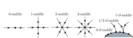
Figure 2. Multi-saddles.

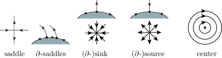
Figure 3. A saddle, two $\partial$-saddles, a sink, a $\partial$-sink, a source, a $\partial$-source, and a center

2.2.2. Multi-saddle separatrices

A separatrix is a multi-saddle separatrix if it is from and to multi-saddles.

2.2.3. Sectors for flows on surfaces

The restriction $v|_{A}$ for a subset $A$ is a sector for a singular point $x$ if there are a non-degenerate interval $I\subseteq[0,2\pi)$ and a homeomorphism $h\colon\{x\}\sqcup A\to\{0\}\sqcup\{(r\cos\theta,r\sin\theta)\in\mathbb{R}^{2}\mid r\in(0,1),\theta\in I\}$ such that $h^{-1}(0)=x$.

Definition 5.

A parabolic sector is topologically equivalent to a flow box with the point $(\pm\infty,0)$ as on the left of Figure 4.

Definition 6.

A hyperbolic (resp. elliptic) sector is topologically equivalent to a Reeb component with the point $(\infty,0)$ (resp. $(-\infty,0)$) as on the middle (resp. left) of Figure 4.

Figure 4. Two parabolic sectors $P^{-}$ and $P^{+}$, two hyperbolic sectors $H^{-}$ and $H^{+}$ with clockwise and anti-clockwise orbit directions, and two elliptic sectors $E^{+}$ and $E^{-}$ with clockwise and anti-clockwise orbit directions, respectively.

A separatrix is a hyperbolic (resp. elliptic, parabolic) border separatrix if it is contained in the boundary of a hyperbolic sector (resp. a maximal open elliptic sector, a maximal open parabolic sector).

Definition 7.

A singular point in the interior of the surface is finitely sectored if either it is a center or there is its open neighborhood which is an open disk and is a finite union of the point, parabolic sectors, hyperbolic sectors, and elliptic sectors such that a pair of distinct sectors intersects at most two orbit arcs.

A singular point on the boundary of the surface is finitely sectored if it is finitely sectored for the resulting flow on the double of the compact surface. Notice that quasi-regularity implies that each singular point is a finitely sectored singular point without elliptic sectors. A singular point is a multi-saddle if and only if it is a finitely sectored singular point whose sectors are hyperbolic. Similarly, a singular point is a sink, a $\partial$-sink, a source, or a $\partial$-source if and only if it is a finitely sectored singular point whose sectors consist of exactly one parabolic sector as in Figure 3.

In [6, Theorem A], any isolated singular points of a gradient flow on a surface are characterized as non-trivial finitely sectored singular points without elliptic sectors.

2.2.4. Morse-Smale-like flows on surfaces

We introduce Morse-Smale-like flows to describe gradient flows and “gradient flows with limit cycles” as follows.

Definition 8.

A flow $v$ of weakly finite type is Morse-Smale-like if it satisfies the following four conditions:
(1) Each recurrent orbit is closed.
(2) There are at most finitely many limit cycles.
(3) Each singular point is finitely sectored.
(4) The set of non-recurrent points is open dense in $S$.

In [6, Theorem B], it is shown that a flow on a compact surface is a gradient flow with finitely many singular points if and only if the flow is Morse-Smale-like without elliptic sectors or non-trivial circuits.

2.3. Generic non-gradient and non-Morse-Smale flows on surfaces

Notice that the set of $C^{1}$ gradient flows is not open in the set of $C^{1}$ flows because singular points need not non-degenerate. Moreover, hyperbolic limit cycles for $C^{1}$ flows can be bifurcated into topologically non-hyperbolic limit cycles. However, forbidding the existence of fake limit cycles (see definition below), fixing the sum of indices of sources, sinks, $\partial$-sources, and $\partial$-sinks, and fixing the number of limit cycles, we topologically characterize codimension $k$ flows of gradient flows and of Morse-Smale-like flows in this paper.

2.3.1. Fake limit cycle, a fake multi-saddle, and a fake parabolic sector

We define a fake limit cycle, a fake multi-saddle, and a fake parabolic sector as follows.

Definition 9.

A limit cycle is a fake limit cycle if it is semi-attracting on one side and semi-repelling on another side as in Figure 5.

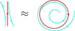
Figure 5. Fake limit cycle

Definition 10.

A singular point is a fake multi-saddle if it is either a $0$-saddle or a $0$-$\partial$-saddle as in Figure 3.

Definition 11.

A parabolic sector $A$ for a singular point $x$ is fake if there are hyperbolic border separatrices $\gamma,\mu$ from/to $x$ such that $A$ is transversely bounded by $\gamma,\mu$ as in Figure 6.

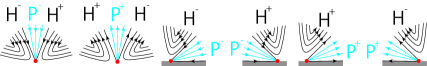
Figure 6. Fake parabolic separatrices

Roughly speaking, a fake parabolic sector is a parabolic sector either between two hyperbolic sectors or between one hyperbolic sector and a boundary component. [6, Theorem A] implies that a gradient flow with isolated singular points on a surface is quasi-regular if and only if there are no fake parabolic sectors.

2.3.2. Subspaces

For any $r\in\mathbb{Z}_{\geq 0}\sqcup\{\infty\}$, let $\mathcal{G}^{r}_{>-1}(S)$ be the set of $C^{r}$ gradient flows with finitely many singular points without fake multi-saddles or fake parabolic sectors on a compact surface $S$. Equip $\mathcal{G}^{r}_{>-1}(S)$ with the $C^{r}$ topology. For any $k_{-},k_{+}\in\mathbb{Z}_{>0}$, denote by $\mathcal{G}^{r}_{k_{-}/2,k_{+}/2,>-1}(S)\subseteq\mathcal{G}^{r}_{>-1}(S)$ the subset of quasi-regular gradient flows whose sums of indices of sinks and $\partial$-sinks (resp. sources and $\partial$-sources) are $k_{-}/2$ (resp. $k_{+}/2$). Notice that the subspace $\mathcal{G}^{r}_{k_{-}/2,k_{+}/2,>-1}(S)$ is a connected component of $\mathcal{G}^{r}_{>-1}(S)$ under non-existence of creations and annihilations of singular points. For any $q_{1},q_{2}\in\mathbb{Z}_{\geq 0}$, denote by $\mathcal{G}^{r}_{k_{-}/2,k_{+}/2,q}(S;q_{1},q_{2})\subseteq\mathcal{G}^{r}_{k_{-}/2,k_{+}/2,>-1}(S)$ the subset of gradient flows in $\mathcal{G}^{r}_{k_{-}/2,k_{+}/2,>-1}(S)$ such that

$$q_{1}:=\sum_{i\geq 2}(i-1)(2\#\{i\text{-saddle}\}+\#\{i/2\text{-}\partial\text{-saddle}\})$$

and $q_{2}$ is the number of multi-saddle separatrices outside of the boundary $\partial S$. For any $q\in\mathbb{Z}_{\geq 0}$, put

$$\mathcal{G}^{r}_{k_{-}/2,k_{+}/2,q}(S):=\bigcup_{q_{1}=0}^{q}\mathcal{G}^{r}_{k_{-}/2,k_{+}/2,q}(S;q_{1},q-q_{1})$$

and $\mathcal{G}^{r}_{k_{-}/2,k_{+}/2,>q}(S):=\bigcup_{q^{\prime}>q}\mathcal{G}^{r}_{k_{-}/2,k_{+}/2,q^{\prime}}(S)$. A flow in $\mathcal{G}^{r}_{k_{-}/2,k_{+}/2,q}(S)$ is called of codimension $q$.

2.3.3. Whitehead moves

A collapsing of a heteroclinic separatrix and the inverse operation as in Figure 7 are called the Whitehead moves. A perturbation preserves multi-saddles if there are neither merges nor splitting of multi-saddles.

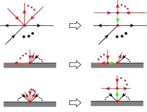
Figure 7. Whitehead moves: splittings of multi-saddles

3. Combinatrial structure of the space of gradient flows

In this section, we have the following hierarchical structure.

Theorem 3.1.

For any $r\in\mathbb{Z}_{>0}\sqcup\{\infty\}$, any integers $k_{-},k_{+}\in\mathbb{Z}_{>0}$ and any $q\in\mathbb{Z}_{\geq-1}$, the subspace $\mathcal{G}^{r}_{k_{-}/2,k_{+}/2,q+1}(S)$ is open dense in the space $\mathcal{G}^{r}_{k_{-}/2,k_{+}/2,>q}(S)$ and consists of structurally stable in $\mathcal{G}^{r}_{k_{-}/2,k_{+}/2,>q}(S)$.

To show the previous theorem, we state the following three lemmas. First, we have the following observation.

Lemma 3.2.

The following statements hold for any small perturbations in the subspace $\mathcal{G}^{r}_{k_{-}/2,k_{+}/2,>-1}(S)$:
(1) Any attracting or repelling singular points (i.e. sinks, $\partial$-sinks, sources, and $\partial$-sources) are preserved under the perturbations.
(2) No attracting or repelling singular points are created or annihilated by the perturbations.
(3) Any splittings of singular points by the perturbations are those of multi-saddles into multi-saddles.
(4) No multi-saddles are created or annihilated by the perturbations.

Proof.

Note that each singular point of any flows in $\mathcal{G}^{r}_{k_{-}/2,k_{+}/2,>-1}(S)$ is either a multi-saddle, a sink, a source, a $\partial$-sink, or a $\partial$-source. Fix a flow $v$ in the subspace $\mathcal{G}^{r}_{k_{-}/2,k_{+}/2,>-1}(S)$. Let $x_{1},\ldots,x_{k}$ be the attracting and repelling singular points of $v$, $y_{1},\ldots,y_{l}$ the multi-saddles of $v$, $U_{i}$ small closed disks which are isolated neighborhoods of $x_{i}$ respectively, and $V_{j}$ small closed disks which are isolated neighborhoods of $y_{j}$ respectively such that $U_{i}$ and $V_{j}$ are pairwise disjoint. Then any small perturbations of $v$ in $\mathcal{G}^{r}_{k_{-}/2,k_{+}/2,>-1}(S)$ preserves the sum of indices of singular points in any $U_{i}$. By the quasi-regularity of $\mathcal{G}^{r}_{k_{-}/2,k_{+}/2,>-1}(S)$, the sum of indices of attracting or repelling singular points on any $U_{i}$ is non-decreasing by any small perturbations of $v$ in $\mathcal{G}^{r}_{k_{-}/2,k_{+}/2,>-1}(S)$. Since the sum of indices of attracting or repelling singular points is $k_{-}/2+k_{+}/2$, the sum of indices of attracting or repelling singular points on any $U_{i}$ is non-increasing and so preserved by any small perturbations of $v$ in $\mathcal{G}^{r}_{k_{-}/2,k_{+}/2,>-1}(S)$. This implies that there are no attracting or repelling singular points outside of $\bigsqcup_{i}U_{i}$. Therefore any singular points in the disjoint union $\bigsqcup_{j}V_{j}$ are multi-saddles. This means that there are no creations of attracting or repelling singular points by any small perturbations in $\mathcal{G}^{r}_{k_{-}/2,k_{+}/2,>-1}(S)$, and that any splittings of singular points by any small perturbations in $\mathcal{G}^{r}_{k_{-}/2,k_{+}/2,>-1}(S)$ are those of multi-saddles into multi-saddles. Since no creations of attracting or repelling singular points by any small perturbations in $\mathcal{G}^{r}_{k_{-}/2,k_{+}/2,>-1}(S)$, by Poincaré-Hopf theorem and the non-existence of fake multi-saddles, there are neither creations nor annihilations of multi-saddles by any small perturbations in $\mathcal{G}^{r}_{k_{-}/2,k_{+}/2,>-1}(S)$. ∎

The previous lemma implies that any merges as in Figure 8 are forbidden.

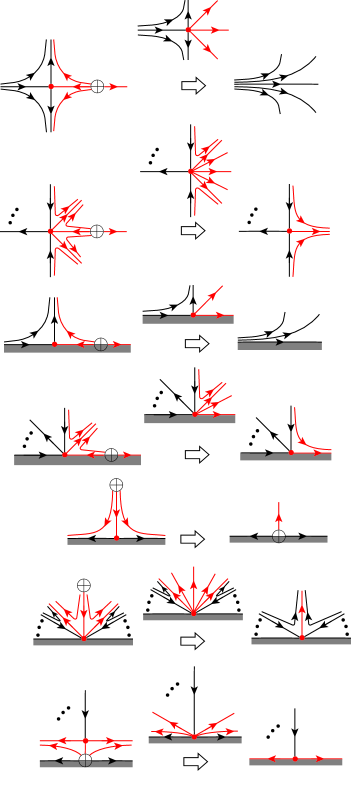
Figure 8. Forbidden merges of multi-saddles and attracting singular points in $\mathcal{G}^{r}_{k_{-}/2,k_{+}/2,>-1}(S)$

We have the following density.

Lemma 3.3.

For any $r\in\mathbb{Z}_{>0}\sqcup\{\infty\}$, any integers $k_{-},k_{+}\in\mathbb{Z}_{>0}$ and any $q\in\mathbb{Z}_{\geq-1}$, the subspace $\mathcal{G}^{r}_{k_{-}/2,k_{+}/2,q+1}(S)$ is dense in the space $\mathcal{G}^{r}_{k_{-}/2,k_{+}/2,>q}(S)$.

Proof.

By [6, Theorem G], the assertion holds for $p=-1$. We may assume that $p\geq 0$. It suffices to show that the space $\mathcal{G}^{r}_{k_{-}/2,k_{+}/2,q+1}(S)$ is dense in $\mathcal{G}^{r}_{k_{-}/2,k_{+}/2,q+1}(S)\sqcup\mathcal{G}^{r}_{k_{-}/2,k_{+}/2,q+2}(S)$. Fix a flow $v\in\mathcal{G}^{r}_{k_{-}/2,k_{+}/2,q+2}(S)$. If $v$ has multi-saddle separatrices outside of the boundary $\partial S$, then one can perturb $v$ into the resulting flow in $\mathcal{G}^{r}_{k_{-}/2,k_{+}/2,q}(S)$ by cutting exactly one multi-saddle separatrix. Thus we may assume that $v$ has no multi-saddle separatrices outside of the boundary $\partial S$. Then there is a multi-saddle $x$. [6, Lemma 9.2] implies that there is a small perturbation of $v$ whose resulting flow is contained in $\mathcal{G}^{r}_{k_{-}/2,k_{+}/2,q+1}(S)\sqcup\mathcal{G}^{r}_{k_{-}/2,k_{+}/2,q+2}(S)$. ∎

We have the following openness and stability.

Lemma 3.4.

For any $r\in\mathbb{Z}_{>0}\sqcup\{\infty\}$, any integers $k_{-},k_{+}\in\mathbb{Z}_{>0}$ and any $q\in\mathbb{Z}_{\geq-1}$, the subspace $\mathcal{G}^{r}_{k_{-}/2,k_{+}/2,q+1}(S)$ is open in the space $\mathcal{G}^{r}_{k_{-}/2,k_{+}/2,>q}(S)$ and consists of structurally stable in $\mathcal{G}^{r}_{k_{-}/2,k_{+}/2,>q}(S)$.

Proof.

By [6, Theorem G], the assertion holds for $p=-1$. We may assume that $p\geq 0$. Fix a flow $v\in\mathcal{G}^{r}_{k_{-}/2,k_{+}/2,>q}(S)$. By the same arguments of the proofs of [6, Lemma 7.4 and Lemma 7.5], any small perturbation of $v$ in $\mathcal{G}^{r}_{k_{-}/2,k_{+}/2,>q}(S)$ preserving singular points makes no new multi-saddles separatrices. Denote by $x_{1},\ldots,x_{n},x_{n+1},\ldots,x_{n+m}$ the multi-saddles such that $x_{j}$ for any $j\in\{1,\ldots,n\}$ is a $k_{j}$-saddle and that $x_{n+j}$ for any $j\in\{1,\ldots,m\}$ is a $k_{n+j}/2$-$\partial$-saddle of $v$. Let $w$ be a flow obtained by a small perturbation of $v$ in $\mathcal{G}^{r}_{k_{-}/2,k_{+}/2,>q}(S)$. By [6, Lemma 7.2 and Lemma 7.3], there are small isolated neighborhood $U_{x_{j}}$ of $x_{j}$ for any $j\in\{1,\ldots,n+m\}$ which is an open disk and intersects no multi-saddle separatrices except multi-saddle separatrices from or to $x_{j}$ such that $\mathrm{ind}_{v}(U_{x_{j}})=\mathrm{ind}_{w}(U_{x_{j}})$. This implies that the continuation of $x_{j}$ for any $j\in\{1,\ldots,n\}$ (resp. $j\in\{n+1,\ldots,n+m\}$) is finitely many points $x_{j,1},\ldots,x_{j,l_{j}}$ (resp. $x_{j,1},\ldots,x_{j,l^{\prime}_{j}},x_{j,1},\ldots,x_{j,l^{\prime}_{j}+l^{\prime\prime}_{j}}$) with $k_{j}=\sum_{i=1}^{l_{j}}k_{j,i}$ (resp. $k_{j}=\sum_{i=1}^{l^{\prime}_{j}}2k_{j,i}+\sum_{i=1}^{l^{\prime}_{j}}k_{j,i}$) such that $x_{j,i}$ are $k_{j,i}$-saddles (resp. $x_{j,i}$ for any $i\in\{1,l^{\prime}_{j}\}$ are $k_{j,i}$-saddles and $x_{j,l^{\prime}_{j}+i}$ for any $i\in\{1,l^{\prime\prime}_{j}\}$ are $k_{j,l^{\prime}_{j}+i}/2$-$\partial$-saddles). Since $U_{x_{j}}$ is simply connected and $w$ is gradient, the multi-saddle connections containing the multi-saddles $x_{j,i}$ have no loops in $U_{x_{j}}$ and so contain at most $l_{j}-1$ (resp. $l^{\prime}_{j}+l^{\prime\prime}_{j}-1$) multi-saddle separatrices outside of the boundary $\partial S$ in $U_{x_{j}}$, because any trees with $n$ vertices have exactly $n-1$ edges. Then $q_{2}(w)-q_{2}(v)\leq\sum_{j=1}^{n}(l_{j}-1)+\sum_{j=n+1}^{n+m}(l^{\prime}_{j}+l^{\prime\prime}_{j}-1)$. By the inequality $2(k_{j}-1)=2l_{j}-2+\sum_{i=1}^{l_{j}}2(k_{j,i}-1)\geq l_{j}-1+\sum_{i=1}^{l_{j}}2(k_{j,i}-1)$ (resp. $k_{j}-1=2l^{\prime}_{j}+l^{\prime\prime}_{j}-1+\sum_{i=1}^{l^{\prime}_{j}}2(k_{j,i}-1)+\sum_{i=1}^{l^{\prime\prime}_{j}}(k_{j,l^{\prime}_{j}+i}-1)\geq l^{\prime}_{j}+l^{\prime\prime}_{j}-1+\sum_{i=1}^{l^{\prime}_{j}}2(k_{j,i}-1)+\sum_{i=1}^{l^{\prime\prime}_{j}}(k_{j,l^{\prime}_{j}+i}-1)$), we have

$$\begin{split}q_{1}(v)&=\sum_{j=1}^{n}2(k_{j}-1)+\sum_{j=n+1}^{n+m}(k_{j}-1)\\ &\geq\sum_{j=1}^{n}\left(l_{j}-1+\sum_{i=1}^{l_{j}}2(k_{j,i}-1)\right)\\ &+\sum_{j=n+1}^{n+m}\left(l^{\prime}_{j}+l^{\prime\prime}_{j}-1+\sum_{i=1}^{l^{\prime}_{j}}2(k_{j,i}-1)+\sum_{i=1}^{l^{\prime\prime}_{j}}(k_{j,l^{\prime}_{j}+i}-1)\right)\\ &=q_{1}(w)+\sum_{j=1}^{n}(l_{j}-1)+\sum_{j=n+1}^{n+m}(l^{\prime}_{j}+l^{\prime\prime}_{j}-1)\\ &\geq q_{1}(w)+q_{2}(w)-q_{2}(v)\end{split}$$

and so the codimension of $w$ is no more than one of $v$. The equality $q_{1}(v)+q_{2}(v)=q_{1}(w)+q_{2}(w)$ holds for only $n,m\in\{0,1\}$. This means that $v\in\mathcal{G}^{r}_{k_{-}/2,k_{+}/2,q+1}(S)$ if and only if $v$ is preserved under any small perturbations in $\mathcal{G}^{r}_{k_{-}/2,k_{+}/2,>q}(S)$. Therefore $v$ is structurally stable in $\mathcal{G}^{r}_{k_{-}/2,k_{+}/2,>q}(S)$. Moreover, the subspace $\mathcal{G}^{r}_{k_{-}/2,k_{+}/2,q+1}(S)$ is open in the space $\mathcal{G}^{r}_{k_{-}/2,k_{+}/2,>q}(S)$. ∎

Lemma 3.3 and Lemma 3.4 imply Theorem 3.1. Notice that the similar statement holds for quasi-regular Morse-Smale-like flows under the non-existence of fake limit cycles because quasi-regular Morse-Smale-like flows are quasi-Morse-Smale (i.e the resulting flows obtained from quasi-regular gradient flows by replacing singular points with limit cycles and pasting limit cycles) (see [6] for definition details). We will state the statement in the second from the last section more precisely.

4. Abstract cell complex structure and filtration of $\mathcal{G}^{r}_{k_{-}/2,k_{+}/2,>-1}(S)$

In this section, we construct the abstract cell complex structure of the space of gradient flows. The compactness of the surface implies the following finite property.

Lemma 4.1.

For any $r\in\mathbb{Z}_{\geq 0}\sqcup\{\infty\}$, any integers $k_{-},k_{+}\in\mathbb{Z}_{>0}$ and any $q\in\mathbb{Z}_{\geq-1}$, the subspace $\mathcal{G}^{r}_{k_{-}/2,k_{+}/2,q}(S)$ contains at most finitely many topological equivalence classes.

Proof.

Since the number of multi-saddles is bounded, there are at most finitely many multi-saddle connections that appear in $\mathcal{G}^{r}_{k_{-}/2,k_{+}/2,q}(S)$. This implies the finite possible combination obtained by merges of saddle connections and the Whitehead move. ∎

Theorem 3.1 implies the following filtration of the space of gradient vector fields on compact surfaces.

Theorem 4.2.

The following statements hold for any $r\in\mathbb{Z}_{>0}\sqcup\{\infty\}$, any integers $k_{-},k_{+}\in\mathbb{Z}_{>0}$ and any $q\in\mathbb{Z}_{\geq-1}$:
(1) $\mathcal{G}^{r}_{k_{-}/2,k_{+}/2,>-1}(S)\supset\mathcal{G}^{r}_{k_{-}/2,k_{+}/2,>0}(S)\supset\mathcal{G}^{r}_{k_{-}/2,k_{+}/2,>1}(S)\supset\cdots$.
(2) The subset $\mathcal{G}^{r}_{k_{-}/2,k_{+}/2,q+1}(S)$ is open dense in $\mathcal{G}^{r}_{k_{-}/2,k_{+}/2,>q}(S)$ and consists of $C^{r}$-structurally stable gradient flows in $\mathcal{G}^{r}_{k_{-}/2,k_{+}/2,>q}(S)$.

4.1. Abstract cell complex structure

4.1.1. Abstract cell complex

For a set $S$ with a transitive relation $\prec$ and a function $\dim\colon S\to\mathbb{Z}_{\geq 0}$, the triple $(S,\prec,\dim)$ is an abstract cell complex if $x\prec y$ implies $\dim x<\dim y$. Then $\dim x$ is called the dimension of $x$, and $x$ is call a cell. A $k$-cell is a cell whose dimension is $k$. The codimension of $x$ is $\sup_{y\in S}\dim y-\dim x$. Note that the triple $(S,\prec,\mathrm{codim})$ can determine the dimension and so the abstract cell complex sturucture. For a finite preordered set $(X,\leq)$, the triple $(X,<,\mathop{\mathrm{ht}})$ is an abstract cell complex.

4.1.2. Abstract cell complex structure of the space of gradient flows

For any $r\in\mathbb{Z}_{\geq 0}\sqcup\{\infty\}$, any integers $k_{-},k_{+}\in\mathbb{Z}_{>0}$ and any integer $q\in\mathbb{Z}_{\geq-1}$, denote by $[\mathcal{G}^{r}_{k_{-}/2,k_{+}/2,>q}(S)]$ the quotient space of $\mathcal{G}^{r}_{k_{-}/2,k_{+}/2,>q}(S)$ by the topologically equivalence classes, and by $[\mathcal{G}^{r}_{k_{-}/2,k_{+}/2,q}(S)]$ the quotient space of $\mathcal{G}^{r}_{k_{-}/2,k_{+}/2,q}(S)$ by the topological equivalence classes.

Lemma 4.1 and Theorem 4.2 imply that $[\mathcal{G}^{r}_{k_{-}/2,k_{+}/2,>q}(S)]$ is a finite $T_{0}$-space, and that the coheight of $[\mathcal{G}^{r}_{k_{-}/2,k_{+}/2,q}(S)]$ corresponds to the codimension as follows.

Theorem 4.3.

The following statements hold for any $r\in\mathbb{Z}_{>0}\sqcup\{\infty\}$, any integers $k_{-},k_{+}\in\mathbb{Z}_{>0}$ and any $q\in\mathbb{Z}_{\geq-1}$:
(1) The subset $[\mathcal{G}^{r}_{k_{-}/2,k_{+}/2,>-1}(S)]$ is a finite $T_{0}$-space and is an abstract cell complex with respect to the opposite order of the specialization preorder and the codimension.
(2) $\overline{[\mathcal{G}^{r}_{k_{-}/2,k_{+}/2,>-1}(S)]_{q+1}}=[\mathcal{G}^{r}_{k_{-}/2,k_{+}/2,>-1}(S)]_{\geq q+1}=[\mathcal{G}^{r}_{k_{-}/2,k_{+}/2,>q}(S)]$.

5. Non-contractibility of the space of gradient flows

In this section, we demonstrate the non-contractibility of a connected component of the space of gradient flows.

5.1. Topological properties of the spaces of gradient flows on compact surfaces

We obtain the negative answer to Question 1. More precisely, we have the following statement.

Theorem 5.1.

The connected components of the quotient space $[\mathcal{G}^{r}_{>-1}(S)]$ for any $r\in\mathbb{Z}_{>0}\sqcup\{\infty\}$ are not contractible in general.

In fact, we will show that the quotient space $[\mathcal{G}^{r}_{1,2,>-1}(\Sigma_{0,2})]$ has a connected component which is the weak homotopy type of a bouquet $\mathbb{S}^{2}\vee\mathbb{S}^{2}$ of two two-dimensional spheres, where $\Sigma_{g,p}$ is the closed orientable surface with genus $g$ and $p$ punctures. On the other hand, we have the following observation.

Proposition 5.2.

For any $r\in\mathbb{Z}_{>0}\sqcup\{\infty\}$ and any integers $k_{-},k_{+}\in\mathbb{Z}_{>0}$, the subspace $[\mathcal{G}^{r}_{k_{-}/2,k_{+}/2,>-1}(\Sigma_{g,0})]$ is contractible or empty.

To show the statements, we recall the theory of homotopy types of finite $T_{0}$-spaces as follows.

5.2. Homotopy types of finite $T_{0}$-spaces

From now on, we equip a finite $T_{0}$-space $(X,\tau)$ with the specialization preorder $\leq_{\tau}$. Notice that $x\leq_{\tau}y$ if and only if $x\in\overline{\{y\}}$. Write the upset $\mathop{\uparrow}_{\tau}x:=\{y\in X\mid x\leq_{\tau}y\}$ and the downset $\mathop{\downarrow}_{\tau}x:=\{y\in X\mid y\leq_{\tau}x\}$. Notice that $\mathop{\downarrow}_{\tau}x-\{x\}=\{y\in X\mid y<_{\tau}x\}$ and $\mathop{\uparrow}_{\tau}x-\{x\}=\{y\in X\mid x<_{\tau}y\}$. To state the characterization of contractibility, we recall beat points as follows [9, 19].

Definition 12.

A point $x\in X$ is a down beat point (or a colinear point ) if there is a point $z\in X$ with $\mathop{\downarrow}_{\tau}x-\{x\}=\mathop{\downarrow}_{\tau}z$.

Definition 13.

A point $x\in X$ is a up beat point (or a linear point ) if there is a point $z\in X$ with $\mathop{\uparrow}_{\tau}x-\{x\}=\mathop{\uparrow}_{\tau}z$.

Definition 14.

A point is a beat point if it is a down or up beat point.

Notice that a point $x\in X$ is a beat point if and only if there is a point $z\in X$ such that either $\mathop{\uparrow}_{\tau}x-\{x\}=\mathop{\uparrow}_{\tau}z$ or $\mathop{\downarrow}_{\tau}x-\{x\}=\mathop{\downarrow}_{\tau}z$, and that the inclusion $X-\{x\}\to X$ for any beat point $x\in X$ is a strong deformation retract.

A finite $T_{0}$-space without beat points is called a minimal finite space. A minimal finite space is a core of a finite $T_{0}$-space $X$ if it is a strong deformation retract of $X$. In [19, Theorem 4], Stong proved that any finite $T_{0}$-space has the unique core up to homeomorphism and that two finite $T_{0}$-spaces are homotopy equivalent to each other if and only if their cores are homeomorphic to each other. We also recall weak beat points [4, 3] as follows.

Definition 15.

A point $x\in X$ is a down weak point if $\mathop{\downarrow}_{\tau}x-\{x\}$ is contractible.

Definition 16.

A point $x\in X$ is a up beat point if $\mathop{\uparrow}_{\tau}x-\{x\}$ is contractible.

Definition 17.

A point is a weak beat point (or a weak point ) if it is a down or up weak point.

Notice that a point $x\in X$ is a weak beat point if and only if either $\mathop{\uparrow}_{\tau}x-\{x\}$ or $\mathop{\downarrow}_{\tau}x-\{x\}$ is contractible, and that the inclusion $X-\{x\}\to X$ for any weak beat point $x\in X$ is a weak homotopy equivalence [4, Proposition 3.3].

5.3. Contractibility of $[\mathcal{G}^{r}_{k_{-}/2,k_{+}/2,>-1}(\Sigma_{g,0})]$

We demonstrate the contractibility of some connected components as follows.

Proof of Proposition 5.2.

Fix any $r\in\mathbb{Z}_{>0}\sqcup\{\infty\}$ and any integers $k_{-},k_{+}\in\mathbb{Z}_{>0}$ such that $[\mathcal{G}^{r}_{k_{-}/2,k_{+}/2,>-1}(\Sigma_{g,0})]$ is not empty. Since $\Sigma_{g,0}$ is a closed surface, every singular point is either a sink, a source, or an $k$-saddle for some $k\in\mathbb{Z}_{>0}$. Put $k:=\chi(\Sigma_{g,0})-(k_{+}+k_{-})/2$. If $k=0$, then there are no multi-saddles and so the component $[\mathcal{G}^{r}_{k_{-}/2,k_{+}/2,>-1}(\Sigma_{g,0})]$ is a singleton. Thus we may assume that $k>0$. Then the topological equivalence class of a flow with a $k$-saddle is the unique maximal element of $[\mathcal{G}^{r}_{k_{-}/2,k_{+}/2,>-1}(\Sigma_{g,0})]$. Since the second maximal elements are up beat points, by induction, the space $[\mathcal{G}^{r}_{k_{-}/2,k_{+}/2,>-1}(\Sigma_{g,0})]$ is contractible. ∎

5.4. Non-contractibility of $[\mathcal{G}^{r}_{1,2,>-1}(\Sigma_{0,2})]$

We have the following statement.

Proposition 5.3.

The quotient space $[\mathcal{G}^{r}_{1,2,>-1}(\Sigma_{0,2})]$ had a connected component which is weakly homotopic to a bouquet $\mathbb{S}^{2}\vee\mathbb{S}^{2}$ of two two-dimensional spheres.

The previous proposition implies Theorem 5.1. To demonstrate the previous proposition, we introduce a notation and show some technical statements as follows.

5.4.1. Connected components

For any non-negative integer $k_{-,1},k_{-,1},k_{+,1},k_{+,2}\in\mathbb{Z}_{\geq 0}$, denote by $\mathcal{G}^{r}_{k_{-,1},k_{-,1}/2,k_{+,1},k_{+,2}/2,>-1}(S)\subset\mathcal{G}^{r}_{k_{-}/2,k_{+}/2,>-1}(S)$ the subset of flows in $\mathcal{G}^{r}_{k_{-}/2,k_{+}/2,>-1}(S)$ whose sums of indices of sinks (resp. $\partial$-sinks, sources, $\partial$-sources) are $k_{-,1}$ (resp. $k_{-,1}/2,k_{+,1},k_{+,2}/2$). By Lemma 3.2, the subspace $\mathcal{G}^{r}_{k_{-,1},k_{-,1}/2,k_{+,1},k_{+,2}/2,>-1}(S)$ is a connected component of $\mathcal{G}^{r}_{k_{-}/2,k_{+}/2,>-1}(S)$.

5.4.2. Non-contractible connected component

Since any flows in $[\mathcal{G}^{r}_{1,0,2,0,0}(\Sigma_{0,2})]$ have a sink, we can consider that the sink is the point at infinity and so that such flows can be identified with flows on the plane $\mathbb{R}^{2}$. To demonstrate the previous proposition, we have the following statements.

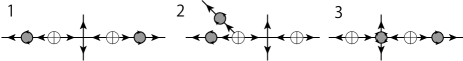
Figure 9. Codimension zero elements in $[\mathcal{G}^{r}_{1,0,2,0,>-1}(\Sigma_{0,2})]$.

Lemma 5.4.

The following statements hold for any flow in $[\mathcal{G}^{r}_{1,2,>-1}(\Sigma_{0,2})]$:
(1) Two separatrices from a saddle or a boundary component connect from two different sources.
(2) The resulting surface of $\Sigma_{0,2}$ removing a sink can be considered as a two-punctured plane.
(3) The sum of indices of multi-saddle is $-3$.
(4) The sum of indices of multi-saddles on a boundary component without $\partial$-sinks or $\partial$-sources is at most $-1$.

Proof.

Assume that two separatrices from a saddle (resp. a boundary component connected from a source) as on the left (resp. right) of Figure 10.

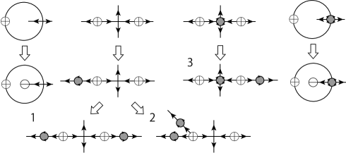
Figure 10. The constructions of combinatorial structures of saddle connections of codimension zero elements.

Then a sink exists in the plane, which contradicts that a sink exists only at the point at infinity. Therefore the assertion (1) holds.

The surface $\Sigma_{0,2}$ is a closed annulus whose Euler characteristic is zero. The resulting surface of $\Sigma_{0,2}$ removing a sink can be considered as a two-punctured plane. This means that the assertion (2) holds.

The singular point set of any flow in $[\mathcal{G}^{r}_{1,2,0}(\Sigma_{0,2})]$ consists of sinks, $\partial$-sinks, sources, $\partial$-sources, and multi-saddles. Since the sum of attracting or repelling singular points is $3$ and the Euler characteristic of any closed annulus is zero, by Poincaré-Hopf theorem, the sum of indices of multi-saddle is $-3$. Therefore the assertion (3) holds.

Since the closed annulus $\Sigma_{0,2}$ has exactly two boundary components, the sum of indices of multi-saddles on a boundary component without $\partial$-sinks or $\partial$-sources is at most $-1$. Therefore the assertion (4) holds.

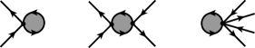
Figure 11. Forbidden boundary components with pinchings in gradient flows.

∎

Lemma 5.5.

Any boundary component for a flow in $[\mathcal{G}^{r}_{1,0,2,0,>-1}(\Sigma_{0,2})]$ is one of the following structures as in Figure 12:
(1) The singular points on it are exactly two $\partial$-saddles.
(2) The singular points on it are exactly four $\partial$-saddles.
(3) The singular points on it are exactly two $\partial$-saddles and one $1$-$\partial$-saddle.
(4) The singular points on it are exactly one $\partial$-saddle and one $3/2$-$\partial$-saddle.

Proof.

Fix a flow in $[\mathcal{G}^{r}_{1,0,2,0,>-1}(\Sigma_{0,2})]$. Since the surface $\Sigma_{0,2}$ has exactly two boundary components, by Lemma 5.4, the sum of indices of multi-saddles on any boundary component is $-1$ or $-2$. Because a boundary component with one singular point and one non-recurrent orbit as on the left of Figure 11 does not appear in any gradient flows, if the sum is $-1$ then the singular points on it are two $\partial$-saddles. Thus we may assume that the sum is $-2$. Since a boundary component with two singular points and two non-recurrent orbits as on the middle or right of Figure 11 does not appear in any gradient flows, the singular points on the boundary are one of the forms in Figure 12.

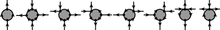
Figure 12. Possible local structures on boundary components in gradient flows in $[\mathcal{G}^{r}_{1,0,2,0,>-1}(\Sigma_{0,2})]$.

∎

Lemma 5.6.

The subspace $[\mathcal{G}^{r}_{1,0,2,0,0}(\Sigma_{0,2})]$ consists of three topological equivalence classes, as in Figure 10.

Proof.

Lemma 5.4(3) implies that the sum of indices of multi-saddle is three. From Lemma 5.5, the set of multi-saddles consists either of six $\partial$-saddles or of one saddle and four $\partial$-saddles. By Lemma 5.4(1), two separatrices from a saddle or a boundary component connect from two different sources. By definition of codimension, there are no multi-saddle separatrices outside of the boundary $\partial\Sigma_{0,2}$. Then we have exactly three possibilities of multi-saddle connections as in the middle of Figure 10. Therefore the codimension zero topological equivalence classes of flows are represented by three structurally stable gradient flows as in Figure 10. ∎

Lemma 5.7.

The subspace $[\mathcal{G}^{r}_{1,0,2,0,1}(\Sigma_{0,2})]$ consists of eight topological equivalence class as in Figure 13.

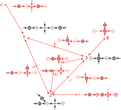
Figure 13. Codimension one elements in $[\mathcal{G}^{r}_{1,0,2,0>-1}(\Sigma_{0,2})]$.

Proof.

From Lemma 5.4(4), the sum of indices of multi-saddles on a boundary component is at most $-1$. By definition of codimension, any codimension one flow has either one pinching or one multi-saddle separatrix outside of the boundary $\partial\Sigma_{0,2}$. From Lemma 5.4(3), the sum of indices of multi-saddles is $-3$.

Suppose that there is exactly one multi-saddle separatrix outside of the boundary. From Lemma 5.4(4), the existence of two boundary components implies that there are at least four $\partial$-saddles. Therefore the set of multi-saddles consists either of six $\partial$-saddles or of one saddle and four $\partial$-saddles. Then there are exactly six codimension one elements with one multi-saddle separatrix outside of the boundary in $[\mathcal{G}^{r}_{1,0,2,0>-1}(\Sigma_{0,2})]$, which are listed in Figure 14.

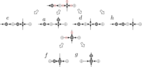
Figure 14. The constructions of codimension one elements with one multi-saddle separatrix outside of the boundary in $[\mathcal{G}^{r}_{1,0,2,0>-1}(\Sigma_{0,2})]$.

Suppose that there is exactly one pinching. Then there are four $\partial$-saddles and one $1$-$\partial$-saddle. Therefore there are two codimension one elements with one pinching in $[\mathcal{G}^{r}_{1,0,2,0>-1}(\Sigma_{0,2})]$ as in Figure 15 by symmetry.

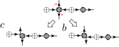
Figure 15. The constructions of codimension one elements with one pinching in $[\mathcal{G}^{r}_{1,0,2,0>-1}(\Sigma_{0,2})]$.

Local perturbations for pinchings and multi-saddle separatices from or to $\partial$-saddles in the subspace $[\mathcal{G}^{r}_{1,0,2,0>-1}(\Sigma_{0,2})]$ as on the upper and middle of Figure 16 imply codimension zero elements.

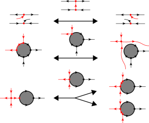
Figure 16. Local perturbations for multi-saddle separatices from or to $\partial$-saddles and local perturbations for pinchings in the subspace $[\mathcal{G}^{r}_{1,0,2,0>-1}(\Sigma_{0,2})]$.

Then we have exactly eight possibilities of multi-saddle connections as in Figure 13. ∎

We list all codimension two elements in $[\mathcal{G}^{r}_{1,0,2,0>-1}(\Sigma_{0,2})]$.

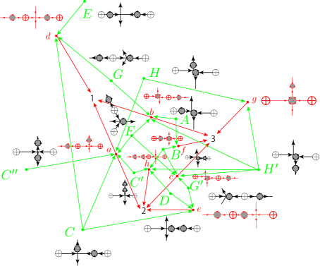
Figure 17. Codimension two elements in $[\mathcal{G}^{r}_{1,0,2,0>-1}(\Sigma_{0,2})]$.

Lemma 5.8.

The subspace $[\mathcal{G}^{r}_{1,0,2,0,2}(\Sigma_{0,2})]$ consists of twelve topological equivalence class as in Figure 17.

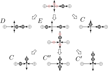
Figure 18. The constructions of codimension two elements with two multi-saddle separatrices outside of the boundary in the subspace $[\mathcal{G}^{r}_{1,0,2,0>-1}(\Sigma_{0,2})]$.

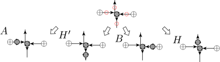
Figure 19. The constructions of codimension two elements with one pinching and one multi-saddle separatrix outside of the boundary in $[\mathcal{G}^{r}_{1,0,2,0>-1}(\Sigma_{0,2})]$.

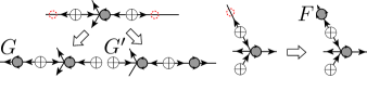
Figure 20. The constructions of codimension two elements with one $3/2$-$\partial$-saddle in $[\mathcal{G}^{r}_{1,0,2,0>-1}(\Sigma_{0,2})]$.

Proof.

By definition of codimension, from Lemma 5.5, any codimension two flow has either exactly one $3/2$-$\partial$-saddle, a pair of one pinching and one multi-saddle separatrix outside of the boundary $\partial\Sigma_{0,2}$, or two multi-saddle separatrices outside of the boundary $\partial\Sigma_{0,2}$. From Lemma 5.4(3), the sum of indices of multi-saddles is $-3$.

Suppose that there are exactly two multi-saddle separatrices outside of the boundary. By Lemma 5.5, the existence of two boundary components implies that there are at least four $\partial$-saddles. Then there are exactly five codimension two elements with two multi-saddle separatrices outside of the boundary in the subspace $[\mathcal{G}^{r}_{1,0,2,0>-1}(\Sigma_{0,2})]$ which are listed in Figure 18.

Suppose that there is exactly one pinching and one multi-saddle separatrix outside of the boundary. By Lemma 5.5, the existence of two boundary components implies that there are four $\partial$-saddles and one $1$-$\partial$-saddle. Then there are exactly four codimension two elements with one pinching and one multi-saddle separatrix outside of the boundary in $[\mathcal{G}^{r}_{1,0,2,0>-1}(\Sigma_{0,2})]$ which are listed in Figure 19.

Suppose that there is exactly one $3/2$-$\partial$-saddle. Then there are exactly three codimension three elements with one $3/2$-$\partial$-saddle in $[\mathcal{G}^{r}_{1,0,2,0>-1}(\Sigma_{0,2})]$ which are listed in Figure 20.

Local perturbations for pinchings and multi-saddle separatices from or to $\partial$-saddles in the subspace $[\mathcal{G}^{r}_{1,0,2,0>-1}(\Sigma_{0,2})]$ as in Figure 16 imply codimension one elements. Then we have exactly twelve possibilities of multi-saddle connections as in Figure 17. ∎

We list all codimension three elements in $[\mathcal{G}^{r}_{1,0,2,0>-1}(\Sigma_{0,2})]$.

Lemma 5.9.

The subspace $[\mathcal{G}^{r}_{1,0,2,0,3}(\Sigma_{0,2})]$ consists of six topological equivalence classes as in Figure 21, each of which is represented by a flow with one $3/2$-$\partial$-saddle and one pinching and one multi-saddle separatrix outside of the boundary.

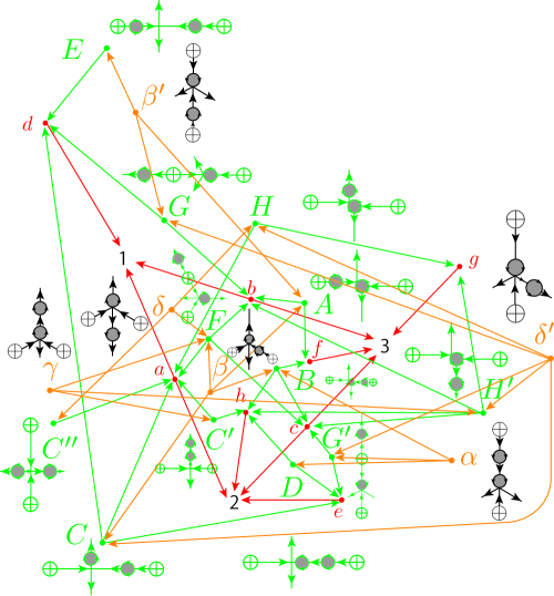
Figure 21. Codimension three elements in $[\mathcal{G}^{r}_{1,0,2,0>-1}(\Sigma_{0,2})]$.

Proof.

By definition of codimension, from Lemma 5.5, any gradient flows whose topological equivalence classes are codimension three has exactly one $3/2$-$\partial$-saddle and one pinching and one multi-saddle separatrix outside of the boundary as in Figure 22. Local perturbations for pinchings and multi-saddle separatices from or to $\partial$-saddles in the subspace $[\mathcal{G}^{r}_{1,0,2,0>-1}(\Sigma_{0,2})]$ as in Figure 16 imply codimension two elements. By listing all the possible combinations, we obtain six multi-saddle connection diagrams as in Figure 21.

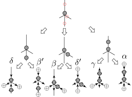
Figure 22. The constructions of codimension three elements in $[\mathcal{G}^{r}_{1,0,2,0>-1}(\Sigma_{0,2})]$.

∎

By the previous three lemmas, we have the following statement.

Lemma 5.10.

The Hesse diagram of the opposite order of the specialization preorder of the finite $T_{0}$-space $[\mathcal{G}^{r}_{1,0,2,0>-1}(\Sigma_{0,2})]$ is shown in Figure 23.

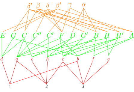
Figure 23. The Hesse diagram $X_{0}$ of the opposite order of the specialization preorder of the finite $T_{0}$-space $[\mathcal{G}^{r}_{1,0,2,0>-1}(\Sigma_{0,2})]$.

Lemma 5.11.

The minimal finite space of the finite $T_{0}$-space $[\mathcal{G}^{r}_{1,0,2,0>-1}(\Sigma_{0,2})]$ is shown in Figure 28 and the space $[\mathcal{G}^{r}_{1,0,2,0>-1}(\Sigma_{0,2})]$ is weak homotopy equivalent to the finite space whose Hessian is shown in Figure 31.

Proof.

The Hesse diagram of the opposite order of the specialization preorder of the finite $T_{0}$-space $[\mathcal{G}^{r}_{1,0,2,0>-1}(\Sigma_{0,2})]$ is shown in Figure 23. Remove up beat points $E$, $C^{\prime\prime}$, $C^{\prime}$, and $D$. Then we have the Hesse diagram as in Figure 24. Remove down beat points $d,e,h,f,$ and $g$. Then we have the Hesse diagram as in Figure 25. Remove down beat points $G$, $C$, $G^{\prime}$, and $A$. Then we have the Hesse diagram as in Figure 26. Remove down beat points $\alpha$, $\beta^{\prime}$, and $B$. Then we have the Hesse diagram as in Figure 27. Remove a down beat point $\beta$. Then we have the Hesse diagram as in Figure 28 which is the core. Remove a down weak point $H^{\prime}$. Then we have the Hesse diagram as in Figure 29. Remove a down beat point $\gamma$. Remove an up beat points $F$. Then we have the Hesse diagram as in Figure 30. Remove an up beat points $a$. Then we have the Hesse diagram as in Figure 31.

This means that $[\mathcal{G}^{r}_{1,0,2,0>-1}(\Sigma_{0,2})]$ is weak homotopy equivalent to the finite space whose Hessian is shown in Figure 31. ∎

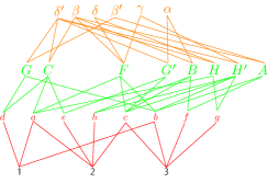
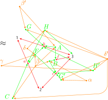
Figure 24. The resulting Hesse diagram $X_{1}$ of the opposite order of the specialization preorder of the resulting diagram of $X_{0}$ by removing $E$, $C^{\prime\prime}$, $C^{\prime}$, and $D$.

Figure 25. The resulting Hesse diagram $X_{2}$ of the opposite order of the specialization preorder of the resulting diagram of $X_{1}$ by removing $d,e,h,f$, and $g$.

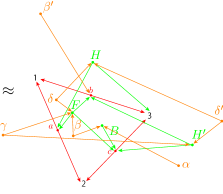
Figure 26. The resulting Hesse diagram $X_{3}$ of the opposite order of the specialization preorder of the resulting diagram of $X_{2}$ by removing $G$, $C$, $G^{\prime}$, and $A$.

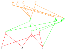
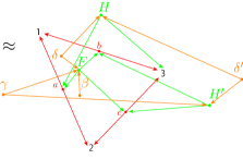
Figure 27. The resulting Hesse diagram $X_{4}$ of the opposite order of the specialization preorder of the resulting diagram of $X_{3}$ by removing $\alpha$, $\beta^{\prime}$, and $B$.

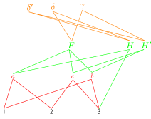
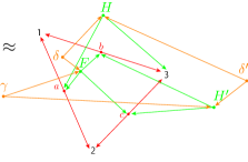
Figure 28. The resulting Hesse diagram $X_{5}$ of the opposite order of the specialization preorder of the resulting diagram of $X_{4}$ by removing $\beta$.

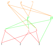
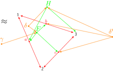
Figure 29. The resulting Hesse diagram $X_{6}$ of the opposite order of the specialization preorder of the resulting diagram of $X_{5}$ by removing the down weak point $H^{\prime}$.

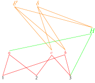
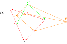
Figure 30. The resulting Hesse diagram $X_{7}$ of the opposite order of the specialization preorder of the resulting diagram of $X_{6}$ by removing $\gamma$, $F$.

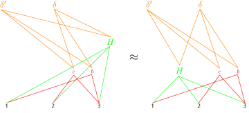
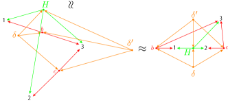
Figure 31. The resulting Hesse diagram $X_{8}$ of the opposite order of the specialization preorder of the resulting diagram of $X_{7}$ by removing $a$.

Lemma 5.12.

The finite $T_{0}$-space $[\mathcal{G}^{r}_{1,0,2,0>-1}(\Sigma_{0,2})]$ is weakly homotopic to a bouquet $\mathbb{S}^{2}\vee\mathbb{S}^{2}$ of two two-dimensional spheres.

Proof.

The order complex $\mathcal{K}(X^{\prime})$ of the finite topological space $X^{\prime}=\{\delta,\delta^{\prime},H,b,c\}$ is homotopy equivalent to a bouquet $\mathbb{S}^{1}\vee\mathbb{S}^{1}$ of two one-dimensional spheres as on the left of Figure 32, and one of the finite topological space $X^{\prime\prime}=\{\delta,\delta^{\prime},H,b,c,1,2\}$ is homotopy equivalent to a closed disk as on the middle of Figure 32. Adding three disks, we obtain the order complex $\mathcal{K}(X_{8})$ of generated by the minimal finite space $X_{8}=\{\delta,\delta^{\prime},H,b,c,1,2,3\}$ is homotopy equivalent to a bouquet $\mathbb{S}^{2}\vee\mathbb{S}^{2}$ as on the right of Figure 32.

From [4, Proposition 3.3], the inclusion $X-\{x\}\to X$ into a finite $T_{0}$-space for any weak beat point $x\in X$ is weak homotopy equivalent. Therefore the subspace $[\mathcal{G}^{r}_{1,0,2,0>-1}(\Sigma_{0,2})]$ is weak homotopy equivalent to $X_{8}$. By [10, Theorem 2], the order complex $\mathcal{K}(X_{8})$ of the finite space $X_{8}$ is weak homotopy equivalent to the finite space $X_{8}$. This implies that the subspace $[\mathcal{G}^{r}_{1,0,2,0>-1}(\Sigma_{0,2})]$ is weak homotopy equivalent to the bouquet $\mathbb{S}^{2}\vee\mathbb{S}^{2}$ of two two-dimensional spheres. ∎

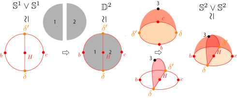
Figure 32. Left, a bouquet $\mathbb{S}^{1}\vee\mathbb{S}^{1}$ of two one-dimensional spheres; middle, a disk; right, a bouquet $\mathbb{S}^{2}\vee\mathbb{S}^{2}$ of two two-dimensional spheres.

The previous lemma implies Proposition 5.3. We could like to ask the following question.

Question 2.

Is every connected component $[\mathcal{G}^{r}_{k_{-,1},k_{-,1},k_{+,1},k_{+,2},>-1}(S)]$ simply connected?

6. Hierarchical structures of the space of Morse-Smale-like flows

We state an analogous statement for Morse-Smale-like flows.

6.1. Combinatrial structure of the space of Morse-Smale-like flows

Recall that a flow on a compact surface is a gradient flow with finitely many singular points if and only if the flow is Morse-Smale-like without elliptic sectors or non-trivial circuits. Therefore Morse-Smale-like flows without elliptic sectors can be considered as “gradient flow with limit circuit” and with finitely many singular points. In this subsection, we describe the topology of the space of “gradient flow with limit cycles” under the non-existence of creations and annihilations of singular points and physical boundaries. Note that any Morse-Smale-like flows without elliptic sectors are quasi-regular.

For any $r\in\mathbb{Z}_{\geq 0}\sqcup\{\infty\}$, denote by $\mathcal{Q}_{**}^{r}(S)$ the set of quasi-regular Morse-Smale-like flows without fake saddles or fake limit cycles. For any $k_{-},k_{+}\in\mathbb{Z}_{\geq 0}$, $r\in\mathbb{Z}_{\geq 0}\sqcup\{\infty\}$, and $l\in\mathbb{Z}_{\geq 0}$, denote by $\mathcal{Q}_{k_{-}/2,k_{+}/2,l,**}^{r}(S)$ the set of quasi-regular Morse-Smale-like flows without fake saddles or fake limit cycles whose sum of indices of attracting (resp. repelling) singular points (i.e. sources and $\partial$-sources (resp. sinks and $\partial$-sinks)) is $k_{-}/2$ (resp. $k_{+}/2$) and whose numbers of limit circuits are $l$. From [6, Theorem F], any flow in $\mathcal{Q}_{k_{-}/2,k_{+}/2,l,**}^{r}(S)$ is quasi-Morse-Smale (i.e resulting flows obtained from quasi-regular gradient flows by replacing singular points with limit cycles and pasting limit cycles).

For any $k_{-},k_{+},l\in\mathbb{Z}_{\geq 0}$, denote by $\mathcal{Q}_{k_{-}/2,k_{+}/2,l,>-1}^{r}(S)\subseteq\mathcal{Q}_{k_{-}/2,k_{+}/2,l,**}^{r}(S)$ the set of flows in $\mathcal{Q}_{k_{-}/2,k_{+}/2,l,**}^{r}(S)$ without non-periodic circuits. Then the subspace $\mathcal{Q}_{k_{-}/2,k_{+}/2,l,>-1}^{r}(S)$ is the set of Morse-Smale-like flows without fake saddles, fake limit cycles, or non-periodic circuits such that the sum of indices of attracting (resp. repelling) singular points (i.e. sources and $\partial$-sources (resp. sinks and $\partial$-sinks)) is $k_{-}/2$ (resp. $k_{+}/2$) and whose numbers of limit circuits are $l$. Notice that the subspace $\mathcal{Q}_{k_{-}/2,k_{+}/2,l,>-1}^{r}(S)$ is a connected component of $\mathcal{Q}_{**}^{r}(S)$ under the non-existence of creations and annihilations of singular points, limit cycles, and boundary components. For any $q_{1},q_{2}\in\mathbb{Z}_{\geq 0}$, denote by $\mathcal{Q}_{k_{-}/2,k_{+}/2,l,q}(S;q_{1},q_{2})\subseteq\mathcal{Q}_{k_{-}/2,k_{+}/2,l,>-1}^{r}(S)$ the subset of flows in $\mathcal{Q}_{k_{-}/2,k_{+}/2,l,>-1}^{r}(S)$ such that

$$q_{1}:=\sum_{i\geq 2}(i-1)(2\#\{i\text{-saddle}\}+\#\{i/2\text{-}\partial\text{-saddle}\})$$

and $q_{2}$ is the number of multi-saddle separatrices outside of the boundary $\partial S$, where $q:=q_{1}+q_{2}$. For any $q\in\mathbb{Z}_{\geq 0}$, put

$$\mathcal{Q}_{k_{-}/2,k_{+}/2,l,q}(S):=\bigcup_{q_{1}=0}^{q}\mathcal{Q}_{k_{-}/2,k_{+}/2,l,q}(S;q_{1},q-q_{1})$$

and $\mathcal{Q}_{k_{-}/2,k_{+}/2,l,>q}(S):=\bigcup_{q^{\prime}>q}\mathcal{Q}_{k_{-}/2,k_{+}/2,l,q^{\prime}}(S)$. A flow in $\mathcal{Q}_{k_{-}/2,k_{+}/2,l,q}(S)$ is called of codimension $q$. Note that $\mathcal{Q}^{r}_{k_{-}/2,k_{+}/2,0,>-1}(S)=\mathcal{G}^{r}_{k_{-}/2,k_{+}/2,>-1}(S)$. Therefore Theorem 5.1 implies the following statement.

Corollary 6.1.

For any $r\in\mathbb{Z}_{>0}\sqcup\{\infty\}$ and any integers $k_{-},k_{+},l\in\mathbb{Z}_{\geq 0}$, the quotient space of $\mathcal{Q}^{r}_{k_{-}/2,k_{+}/2,l,>-1}(S)$ by topologically equivalence classes is not contractible in general.

We have the following hierarchical structure.

Theorem 6.2.

For any $r\in\mathbb{Z}_{>0}\sqcup\{\infty\}$, any integers $k_{-},k_{+},l\in\mathbb{Z}_{\geq 0}$ and any $q\in\mathbb{Z}_{\geq-1}$, the subspace $\mathcal{Q}^{r}_{k_{-}/2,k_{+}/2,l,q+1}(S)$ is open dense in the space $\mathcal{Q}^{r}_{k_{-}/2,k_{+}/2,l,>q}(S)$ and consists of structurally stable in $\mathcal{Q}^{r}_{k_{-}/2,k_{+}/2,l,>q}(S)$.

Theorem 3.1 and the previous theorem are generalizations of [6, Lemma 7.7]. To show the previous theorem, we observe the following statements.

Lemma 6.3.

For any $r\in\mathbb{Z}_{>0}\sqcup\{\infty\}$, any integers $k_{-},k_{+},l\in\mathbb{Z}_{\geq 0}$ and any $q\in\mathbb{Z}_{\geq-1}$, the following statements hold for any small perturbations in the subspace $\mathcal{Q}^{r}_{k_{-}/2,k_{+}/2,l,>-1}(S)$:
(1) Any attracting or repelling singular points (i.e. sinks, $\partial$-sinks, sources, and $\partial$-sources) are preserved under the perturbations.
(2) No attracting or repelling singular points are created or annihilated by the perturbations.
(3) Any splittings of singular points by the perturbations are those of multi-saddles into multi-saddles.
(4) No multi-saddles are created or annihilated by the perturbations.

Proof.

Fix a flow $v$ in $\mathcal{Q}^{r}_{k_{-}/2,k_{+}/2,l,>-1}(S)$. By the finite existence of singular points and limit cycles, since $v$ is a gradient flow, we can take neighborhoods $U_{i}$ and $V_{j}$ in the proof of Lemma 3.2. Since any small neighborhood of singular points of $v$ can be identified with neighborhoods of singular points of a gradient flow in $\mathcal{G}^{r}_{k_{-}/2,k_{+}/2,>-1}(S)$, the proof of Lemma 3.2 also implies the assertion. ∎

Lemma 6.4.

For any $r\in\mathbb{Z}_{>0}\sqcup\{\infty\}$, any integers $k_{-},k_{+},l\in\mathbb{Z}_{\geq 0}$ and any $q\in\mathbb{Z}_{\geq-1}$, any small perturbations in $\mathcal{Q}^{r}_{k_{-}/2,k_{+}/2,l,>-1}(S)$ preserve limit cycles. Moreover, there are neither creations nor annihilations of limit cycles by any small perturbations in $\mathcal{Q}^{r}_{k_{-}/2,k_{+}/2,l,>-1}(S)$.

Proof.

Fix a flow $v$ in $\mathcal{Q}^{r}_{k_{-}/2,k_{+}/2,l,>-1}(S)$. Let $L_{1},\ldots,L_{l}$ be the limit cycles of $v$. By the non-existence of fake limit cycles, the limit cycles $L_{i}$ are topologically hyperbolic (i.e. attracting or repelling). Choose pairwise disjoint closed annuli $A_{i}$ which are neighborhoods of $L_{i}$ with $A_{i}\cap\mathop{\mathrm{Sing}}(v)=\emptyset$ respectively such that the boundaries $\partial A_{i}$ consists of two closed transversals $T_{-,i}$ and $T_{+,i}$. Since the transversality of $C^{r}$ flows is an open condition, any small perturbations in $\mathcal{Q}^{r}_{k_{-}/2,k_{+}/2,l,>-1}(S)$ preserve closed transversals $T_{-,i}$ and $T_{+,i}$. By Lemma 6.3, no attracting or multi-saddles are created or annihilated under any small perturbations in $\mathcal{Q}^{r}_{k_{-}/2,k_{+}/2,l,>-1}(S)$. The quasi-regularity implies that any small perturbations in $\mathcal{Q}^{r}_{k_{-}/2,k_{+}/2,l,>-1}(S)$ create no singular points in $A_{i}$. Let $w$ be the resulting flow from $v$ by a small perturbations in $\mathcal{Q}^{r}_{k_{-}/2,k_{+}/2,l,>-1}(S)$. Then $T_{-,i}$ and $T_{+,i}$ are closed transversals with respect to $w$, and $A_{i}\cap\mathop{\mathrm{Sing}}(w)=\emptyset$. Fix $i\in\{1,\ldots,l\}$. By time reversion if necessary, we may assume that $L_{i}$ is attracting. From the generalization of the Poincaré-Bendixson theorem for a flow with finitely many singular points (cf. [12, Theorem 2.6.1]), the $\omega$-limit set of any point in the annulus $A_{i}$ is a limit cycle. This means that every neighborhoods $A_{i}$ contains exactly one limit cycle, which is topologically hyperbolic, and so is contained in the basin of the attractor or repellor with respect to $w$. Therefore any small perturbations in $\mathcal{Q}^{r}_{k_{-}/2,k_{+}/2,l,>-1}(S)$ preserve limit cycles, and there are neither creations nor annihilations of limit cycles by any small perturbations in $\mathcal{Q}^{r}_{k_{-}/2,k_{+}/2,l,>-1}(S)$. ∎

We demonstrate Thorem 6.2 as follows.

Proof of Thorem 6.2.

By [6, Theorem J], the assertion holds for $p=-1$. We may assume that $p\geq 0$. We claim that the space $\mathcal{Q}^{r}_{k_{-}/2,k_{+}/2,l,q+1}(S)$ is dense in the subspace $\mathcal{Q}^{r}_{k_{-}/2,k_{+}/2,l,>q}(S)$. Indeed, by induction, it suffices to show that the space $\mathcal{Q}^{r}_{k_{-}/2,k_{+}/2,l,q}(S)$ is dense in $\mathcal{Q}^{r}_{k_{-}/2,k_{+}/2,l,q}(S)\sqcup\mathcal{Q}^{r}_{k_{-}/2,k_{+}/2,l,q+1}(S)$. Fix a flow $v\in\mathcal{Q}^{r}_{k_{-}/2,k_{+}/2,l,q+1}(S)$. If $v$ has multi-saddle separatrices outside of the boundary $\partial S$, then one can perturb $v$ into the resulting flow in $\mathcal{Q}^{r}_{k_{-}/2,k_{+}/2,l,q}(S)$ by cutting exactly one multi-saddle separatrix. Thus we may assume that $v$ has no multi-saddle separatrices outside of the boundary $\partial S$. Then there is a multi-saddle $x$. [6, Lemma 8.1] implies that there is a perturbation of $v$ whose resulting flow is contained in $\mathcal{Q}^{r}_{k_{-}/2,k_{+}/2,l,q}(S)$.

We claim that the space $\mathcal{Q}^{r}_{k_{-}/2,k_{+}/2,l,q+1}(S)$ is open in $\mathcal{Q}^{r}_{k_{-}/2,k_{+}/2,l,>q}(S)$. Indeed, it suffices to show that any small perturbation of a flow in $\mathcal{Q}^{r}_{k_{-}/2,k_{+}/2,l,>q}(S)$ does not increase the codimension of the flow. By Lemma 6.4, any small perturbations in $\mathcal{Q}^{r}_{k_{-}/2,k_{+}/2,l,>-1}(S)$ preserve limit cycles. From the proof of Lemma 3.4, the assertion holds. ∎

Theorem 6.2 implies the following finite abstract cell complex structures.

Theorem 6.5.

The following statements hold for any $r\in\mathbb{Z}_{>0}\sqcup\{\infty\}$, any integers $k_{-},k_{+},l\in\mathbb{Z}_{\geq 0}$ and any $q\in\mathbb{Z}_{\geq-1}$:
(1) The quotient space $[\mathcal{Q}^{r}_{k_{-}/2,k_{+}/2,l,q+1}(S)]$ of $\mathcal{Q}^{r}_{k_{-}/2,k_{+}/2,l,q+1}(S)$ by topological equivalence classes is a finite $T_{0}$-space and is an abstract cell complex with respect to the opposite order of the specialization preorder and the codimension.
(2) $\overline{[\mathcal{Q}^{r}_{k_{-}/2,k_{+}/2,l,q+1}(S)]_{q+1}}=[\mathcal{Q}^{r}_{k_{-}/2,k_{+}/2,l,>-1}(S)]_{\geq q+1}=[\mathcal{Q}^{r}_{k_{-}/2,k_{+}/2,l,>q}(S)]$.

7. Final remarks

We state the following future work and the following open question.

7.1. Transition via non-periodic limit circuits between gradient flows and non-gradient Morse-Smale-like flows

Notice that the intermediate flow with a limit circuit must appear between Morse flows and non-Morse Morse-Smale-like flows in $\bigsqcup_{l\geq 0}\mathcal{Q}_{k_{-}/2,k_{+}/2,l,>-1}^{r}(S)$. To state such transitions via saddle connections containing non-periodic limit circuits, we need the “codimension” of the multi-saddle connection diagram for flows in the space $\bigsqcup_{l\geq 0}\mathcal{Q}_{k_{-}/2,k_{+}/2,l,**}^{r}(S)$ like the “codimension” of the multi-saddle connection diagram for Hamiltonian flows [20]. We will report such transitions in the near future.

7.2. Simple connectivity of the space of “gradient flows with limit circuits”

Though we found a non-contractible component for gradient flows, the author does not know whether there exist non-simply-connected connected components for gradient flows and Morse-Smale-like flows. In other words, one would like to know about the following question.

Question 3.

Does the space of topological equivalence classes of gradient flows (or more generally Morse-Smale-like flows) on compact manifolds have non-simply-connected connected components under the non-existence of creations and annihilations of singular points and boundary components?

References

- [1] A. Andronov and L. Pontryagin. Rough systems. In Dokl. Akad. Nauk SSSR, volume 14, pages 247–250, 1937.
- [2] H. Aref and M. Brøns. On stagnation points and streamline topology in vortex flows. Journal of Fluid Mechanics, 370:1–27, 1998.
- [3] J. Barmak and E. Minian. One-point reductions of finite spaces, h–regular cw–complexes and collapsibility. Algebraic & Geometric Topology, 8(3):1763–1780, 2008.
- [4] J. A. Barmak and E. G. Minian. Simple homotopy types and finite spaces. Advances in Mathematics, 218(1):87–104, 2008.
- [5] A. V. Bolsinov and A. T. Fomenko. Integrable Hamiltonian systems: geometry, topology, classification. CRC press, 2004.
- [6] V. Kibkalo and T. Yokoyama. Topological characterizations of morse-smale flows on surfaces and generic non-morse-smale flows. Discrete and Continuous Dynamical Systems, 42(10):4787–4822, 2022.
- [7] R. Kidambi and P. K. Newton. Streamline topologies for integrable vortex motion on a sphere. Physica D: Nonlinear Phenomena, 140(1-2):95–125, 2000.
- [8] T. Ma and S. Wang. Geometric theory of incompressible flows with applications to fluid dynamics. Number 119. American Mathematical Soc., 2005.
- [9] J. May. Finite topological spaces. Notes for REU, 2003.
- [10] M. C. McCord. Singular homology groups and homotopy groups of finite topological spaces. Duke Mathematical Journal, 33(3):465–474, 1966.
- [11] H. Moffatt. The topology of scalar fields in 2d and 3d turbulence. In IUTAM symposium on geometry and statistics of turbulence, pages 13–22. Springer, 2001.
- [12] I. Nikolaev and E. Zhuzhoma. Flows on 2-dimensional manifolds: an overview. Number 1705. Springer Science & Business Media, 1999.
- [13] M. M. Peixoto. Structural stability on two-dimensional manifolds. Topology, 1(2):101–120, 1962.
- [14] T. Sakajo, Y. Sawamura, and T. Yokoyama. Unique encoding for streamline topologies of incompressible and inviscid flows in multiply connected domains. Fluid Dynamics Research, 46(3):031411, 2014.
- [15] T. Sakajo and T. Yokoyama. Transitions between streamline topologies of structurally stable hamiltonian flows in multiply connected domains. Physica D: Nonlinear Phenomena, 307:22–41, 2015.
- [16] T. Sakajo and T. Yokoyama. Tree representation of topological streamline patterns of structurally stable 2D Hamiltonian vector fields in multiply conected domains. The IMA Journal of Applied Mathematics, 83:380–411, 2018.
- [17] T. Sakajo and T. Yokoyama. Discrete representations of orbit structures of flows for topological data analysis. arXiv preprint arXiv:2010.13434, 2020.
- [18] S. Smale. On gradient dynamical systems. Annals of Mathematics, pages 199–206, 1961.
- [19] R. E. Stong. Finite topological spaces. Transactions of the American Mathematical Society, 123(2):325–340, 1966.
- [20] T. Yokoyama. Combinatorial structures of the space of hamiltonian vector fields on compact surfaces. arXiv preprint arXiv:2112.03475, 2021.
- [21] T. Yokoyama and T. Sakajo. Word representation of streamline topologies for structurally stable vortex flows in multiply connected domains. Proceedings of the Royal Society A: Mathematical, Physical and Engineering Sciences, 469(2150):20120558, 2013.
- [22] T. Yokoyama and T. Yokoyama. Complete transition diagrams of generic hamiltonian flows with a few heteroclinic orbits. Discrete Mathematics, Algorithms and Applications, 13(02):2150023, 2021.
- [23] T. Yokoyama and T. Yokoyama. COT representations of 2D Hamiltonian flows and their computable applications, preprint, 2021.