Risk-Sensitive Markov Decision Processes with Long-Run CVaR Criterion

Abstract

CVaR (Conditional Value at Risk) is a risk metric widely used in finance. However, dynamically optimizing CVaR is difficult since it is not a standard Markov decision process (MDP) and the principle of dynamic programming fails. In this paper, we study the infinite-horizon discrete-time MDP with a long-run CVaR criterion, from the view of sensitivity-based optimization. By introducing a pseudo CVaR metric, we derive a CVaR difference formula which quantifies the difference of long-run CVaR under any two policies. The optimality of deterministic policies is derived. We obtain a so-called Bellman local optimality equation for CVaR, which is a necessary and sufficient condition for local optimal policies and only necessary for global optimal policies. A CVaR derivative formula is also derived for providing more sensitivity information. Then we develop a policy iteration type algorithm to efficiently optimize CVaR, which is shown to converge to local optima in the mixed policy space. We further discuss some extensions including the mean-CVaR optimization and the maximization of CVaR. Finally, we conduct numerical experiments relating to portfolio management to demonstrate the main results. Our work may shed light on dynamically optimizing CVaR from a sensitivity viewpoint.

Keywords: Markov decision process, risk-sensitive, long-run CVaR, sensitivity-based optimization, Bellman local optimality equation

1 Introduction

The Markov decision process (MDP) is a fundamental mathematical model used to handle stochastic dynamic optimization problems (Feinberg and Shwartz, 2002; Puterman, 1994). The study of MDPs in operations research is multidisciplinary. It is deeply connected with reinforcement learning in computer science (Kaelbling et al., 1996; Sutton and Barto, 2018), optimal control in control science (Bertsekas, 2005; Lewis et al., 2012), and dynamic discrete choice modeling in econometrics (Aguirregabiria and Mira, 2010; Rust, 1987), etc. Traditional MDP theory focuses on the criteria of discounted or long-run average cost, where the principle of dynamic programming plays a key role. However, for other optimization criteria, such as risk metrics in finance, the corresponding optimization problems usually do not fit the standard MDP model and specific investigations are needed case by case.

Conditional value at risk (CVaR), also called average VaR or expected shortfall, is a widely used risk metric, built upon the VaR and variance related risk metrics (Rockafellar and Uryasev, 2000). We view a continuous random variable $X$ as the stochastic loss and denote its distribution function as $F_{X}(x)$. The CVaR corresponding to this stochastic loss at probability level $\alpha$ is defined as $\mathrm{CVaR}(X):=\mathbb{E}[X|X\geq F_{X}^{-1}(\alpha)]=\frac{1}{1-\alpha}\int_{\alpha}^{1}F_{X}^{-1}(\gamma)d\gamma$, which measures the conditional expectation of losses greater than a given quantile $F_{X}^{-1}(\alpha)$ (or called $\mathrm{VaR}(X)$), where $0<\alpha<1$. Compared with other risk metrics such as variance or VaR, CVaR can measure not only the down-side risk but also the expected value of large losses. Moreover, CVaR is a risk coherent measure (Artzner et al., 1999), which has desirable properties (monotonicity, translation equivariance, sub-additivity, and positive homogeneity).

CVaR has been widely used to measure risk in static (single-stage) optimization problems (Alexander et al., 2006; Fu et al., 2009; Hong et al., 2014). However, it is difficult to handle the CVaR optimization problem in stochastic dynamic (multi-stage) scenarios because of time inconsistency (Boda and Filar, 2006; Pflug and Pichler, 2016). In the MDP terminology, we may define an instantaneous cost function for the long-run CVaR metric as $f(i,a):=F_{X}^{-1}(\alpha)+\frac{1}{1-\alpha}[c(i,a)-F_{X}^{-1}(\alpha)]^{+}$, where $c(i,a)$ is the MDP’s one-step loss incurred at state $i$ with action $a$, $[\cdot]^{+}:=\max\{0,\cdot\}$, and $X$ is the random variable indicating the stochastic loss whose value is realized as $c(i,a)$’s. We can observe that $f(i,a)$ involves $F_{X}^{-1}(\alpha)$ which is affected by future losses and actions. Therefore, the CVaR cost function depends on future behaviors and is not additive or Markovian. The CVaR dynamic optimization problem does not fit a standard MDP model. Thus, the classical Bellman optimality equation does not hold and the principle of dynamic programming fails. Fortunately, Rockafellar and Uryasev (2002) discovered that the $\mathrm{CVaR}$ of the random variable $X$ is equivalent to $\min\limits_{y\in\mathbb{R}}\{y+\frac{1}{1-\alpha}\mathbb{E}[X-y]^{+}\}$, where $y^{*}=F_{X}^{-1}(\alpha)$ exactly achieves the minimum. With this equivalence, Bäuerle and Ott (2011) skillfully converted the CVaR minimization of discounted accumulated costs with finite or infinite horizon into a bilevel optimization problem, where the outer one is a static optimization problem with the auxiliary variable $y\in\mathbb{R}$ and the inner one is a standard MDP with the fixed $y$ and an augmented state space. Although the existence and properties of optimal policies were studied there, the efficient solution of such bilevel MDP problems was not presented. For different values of $y\in\mathbb{R}$, we have to solve different inner MDP problems, which is computationally exhaustive. Such techniques of equivalent MDP transformation and state augmentation were further extended to study the CVaR minimization in other general cases, such as semi-MDPs (Huang and Guo, 2016), continuous-time MDPs (Miller and Yang, 2017), unbounded costs (Uǧurlu, 2017), just to name a few. On the other hand, Haskell and Jain (2015) used occupation measures to study the CVaR optimization of discounted cost infinite-horizon MDPs from the viewpoint of mathematical programming, where the optimality of deterministic policies was also discussed. However, it is usually not efficient to solve a series of mathematical programs, especially when they are not convex or linear programs. Efficiently computing CVaR optimal policies is an important but not well studied topic in the MDP theory.

In the literature, most works study the CVaR of discounted accumulated costs at a terminal stage $T$, say $\mathrm{CVaR}(\tilde{X}_{T})$, where $\tilde{X}_{T}:=\sum_{t=0}^{T}\beta^{t}X_{t}$, $X_{t}$ is the cost at time $t$, and $\beta$ is the discount factor. However, people also care about the cost fluctuation during the procedure, i.e., $\mathrm{CVaR}(X_{t})$ at each time $t$. For example, in financial engineering, a risk-averse investor cannot tolerate high risks during the asset management process, even though the variation of returns at the end of the contract is small. High fluctuations of the asset value may bring anxiety to the risk-averse investor. On the other hand, it is becoming popular to add more inspection points (monthly or even daily) to measure portfolio performance, rather than a single inspection point at the end of the contract. Therefore, the risk measure of procedure behaviors is significant for the theory of MDPs. Compared with the existing works on the steady variance optimization of MDPs (Chung, 1994; Sobel, 1994; Xia, 2020), the steady CVaR measure in MDPs is rarely studied.

In this paper, we study a discrete-time undiscounted MDP with a long-run CVaR criterion. Different from the CVaR metrics for discounted costs, the long-run CVaR measures the conditional expectation of costs when the MDP reaches steady-state. Since the traditional approach of dynamic programming is not applicable for such non-standard MDP problems, we study this problem from the viewpoint of sensitivity-based optimization. By introducing a so-called pseudo CVaR, we derive a bilevel MDP formulation with nested structures, where the inner one is a standard MDP for minimizing the pseudo CVaR. Then, we derive a closed-form difference formula to quantify the difference of long-run CVaR under any two policies. The CVaR difference formula has an elegant form which reduces the difficulty caused by the non-additive CVaR cost function. The optimality of deterministic policies is also shown from the nested formulation. With the CVaR difference formula, we further derive an optimality equation called the Bellman local optimality equation, which describes a necessary and sufficient condition of local optimal policies in the mixed policy space, while is only necessary for global optimal policies. A CVaR derivative formula is also obtained. With the CVaR sensitivity formulas and the Bellman local optimality equation, we develop an iterative algorithm which behaves similarly to the classical policy iteration algorithm and can efficiently converge to local optima. Some interesting extensions are also discussed, including the mean-CVaR optimization problem and the maximization problem of CVaR. Finally, we conduct numerical examples about portfolio management to demonstrate the efficiency of our approach.

The main contributions of this paper have three-fold. First, we study the discrete-time undiscounted MDP with the long-run CVaR criterion. To the best of our knowledge, our paper is the first to investigate MDP theory for minimizing long-run CVaR. Secondly, we derive the CVaR difference and derivative formulas, and the Bellman local optimality equation. Thirdly, we develop a policy iteration-type algorithm, which appears to be much more efficient than solving the bilevel MDP problem studied in the literature (equivalent to solving a series of standard MDPs with the number of MDPs equal to the number of possible values of the outer-tier parameter $y\in\mathbb{R}$). Along with our research direction, we may further develop value iteration-type or policy gradient algorithms, which can enrich the algorithmic study on CVaR dynamic optimization.

The rest of the paper is organized as follows. In Section 2, we give the MDP formulation with the long-run CVaR criterion. In Section 3, we present the main results of this paper, including the CVaR difference formula, the Bellman local optimality equation, iterative algorithms, and the related theorems. In Section 4, we discuss some possible extensions of our results. In Section 5, numerical experiments are conducted to demonstrate our main results. Finally, we conclude this paper and discuss future research topics in Section 6.

2 Problem Formulation

Consider a discrete-time finite MDP with tuple $\langle\mathcal{S},\mathcal{A},\mathcal{P},c\rangle$, where the state space is $\mathcal{S}:=\{1,2,\dots,S\}$ and the action space is $\mathcal{A}:=\{a_{1},a_{2},\dots,a_{A}\}$. A function $\mathcal{P}:\mathcal{S}\times\mathcal{A}\overset{D}{\mapsto}\mathcal{S}$ is the state transition probability kernel with element $p(j|i,a)$, where $\overset{D}{\mapsto}$ represents a mapping to the distribution on the successor $\mathcal{S}$. The element $p(j|i,a)$ indicates the transition probability to state $j$ when action $a$ is adopted at the current state $i$. Obviously, we have $\sum_{j\in\mathcal{S}}p(j|i,a)=1$ for any $i\in\mathcal{S},a\in\mathcal{A}$. We denote $c:\mathcal{S}\times\mathcal{A}\mapsto\mathbb{R}$ as the cost function and its element $c(i,a)$ is the cost incurred at state $i$ with action $a$. In this paper, we limit our discussion to stationary policies which make the associated Markov chains always ergodic (the main results in this paper may be extended to unichain MDPs). A function $d:\mathcal{S}\times\mathcal{A}\mapsto[0,1]$ describes a stationary randomized policy and its element $d(i,a)$ indicates the probability of adopting action $a$ at state $i$, where $\sum_{a\in\mathcal{A}}d(i,a)=1$ for any $i\in\mathcal{S}$. If $d$ is a deterministic policy, we also use $d(i)\in\mathcal{A}$ to indicate the action adopted at state $i$, with a slight abuse of notation. We denote $\mathcal{D}$ and $\mathcal{D}_{0}$ as the space of stationary randomized and deterministic policies, respectively.

We investigate the steady-state behavior of the MDP with policy $d$. We denote $\pi^{d}:\mathcal{S}\times\mathcal{A}\mapsto[0,1]$ as the steady distribution on the space of state-action pairs. We also denote $\pi^{d}(i)=\sum_{a\in\mathcal{A}}\pi^{d}(i,a)$, $i\in\mathcal{S}$. The transition probability matrix of the MDP with policy $d$ is denoted as $P^{d}$ whose element is $P^{d}(i,j)=\sum_{a\in\mathcal{A}}p(j|i,a)d(i,a)$, $i,j\in\mathcal{S}$. By denoting $C^{d}_{t}$ as the instantaneous cost of the MDP at time $t$, we can view $C^{d}_{t}$ as a random variable whose distribution is determined by the initial state distribution $\nu$ and the $t$-step transition probability matrix $(P^{d})^{t}$, i.e., $\nu(P^{d})^{t}$. Obviously, we have $\lim\limits_{t\rightarrow\infty}\nu(P^{d})^{t}=\pi^{d}$ for any $\nu$. Since the MDP is finite, $C^{d}_{t}$ is a discrete random variable with distribution function $F_{C^{d}_{t}}(w)$ and its $\mathrm{CVaR}$ at a probability level $\alpha\in(0,1)$ is defined as below.

$$\mathrm{CVaR}(C^{d}_{t}):=\mathbb{E}\{C^{d}_{t}|C^{d}_{t}\geq F_{C^{d}_{t}}^{-1}(\alpha)\},$$

where $F_{C^{d}_{t}}^{-1}(\alpha)$ is the inverse distribution function of random variable $C^{d}_{t}$, which is also known as its value at risk (VaR) at $\alpha$, or called $\alpha$-quantile

$$F_{C^{d}_{t}}^{-1}(\alpha)=\mathrm{VaR}(C^{d}_{t}):=\inf_{w\in\mathbb{R}}\{w:F_{C^{d}_{t}}(w)\geq\alpha\}.$$

The long-run CVaR of this MDP under policy $d$ is further defined as

$$\mathrm{CVaR}^{d}:=\lim\limits_{T\rightarrow\infty}\frac{1}{T}\sum_{t=0}^{T-1}\mathrm{CVaR}(C^{d}_{t}).$$ (1)

Since the MDP is assumed always ergodic under any policy $d\in\mathcal{D}$, we have

$$\mathrm{CVaR}^{d}=\lim\limits_{t\rightarrow\infty}\mathrm{CVaR}(C^{d}_{t}).$$

Similarly, we also have

$$\mathrm{VaR}^{d}:=\lim\limits_{t\rightarrow\infty}\mathrm{VaR}(C^{d}_{t}).$$ (2)

Our optimization objective is to find the optimal policy $d^{*}$ which attains the minimum of $\mathrm{CVaR}^{d}$, i.e.,

$$\begin{array}[]{rcl}d^{*}&=&\operatorname*{argmin}\limits_{d\in\mathcal{D}}\{\mathrm{CVaR}^{d}\},\\ \mathrm{CVaR}^{*}&=&\min\limits_{d\in\mathcal{D}}\{\mathrm{CVaR}^{d}\}=\mathrm{CVaR}^{d^{*}}.\\ \end{array}$$ (3)

This MDP optimization problem with the long-run CVaR criterion is difficult to handle. To accommodate the CVaR metric, we define a new cost function as

$$\tilde{c}(y,i,a):=y+\frac{1}{1-\alpha}[c(i,a)-y]^{+},\quad\forall i\in\mathcal{S},a\in\mathcal{A},y\in\mathbb{R}.$$ (4)

By denoting $\tilde{c}(y):=(\tilde{c}(y,i,a):i\in\mathcal{S},a\in\mathcal{A})$, we can obtain that the long-run cost of this new MDP $\langle\mathcal{S},\mathcal{A},\mathcal{P},\tilde{c}(y)\rangle$ is

$$\widetilde{\mathrm{CVaR}}^{d}(y)=\lim\limits_{T\rightarrow\infty}\frac{1}{T}\sum_{t=0}^{T-1}\tilde{c}(y,X_{t},A_{t})=\sum_{i\in\mathcal{S},a\in\mathcal{A}}\pi^{d}(i,a)\tilde{c}(y,i,a),$$ (5)

where $X_{t}$ and $A_{t}$ is the system state and action at time $t$, respectively. We call $y$ and $\widetilde{\mathrm{CVaR}}^{d}(y)$ the pseudo VaR and the pseudo CVaR of the MDP, respectively. When $y$ equals the real VaR, then the pseudo CVaR equals the real CVaR of the MDP, i.e.,

$$\mathrm{CVaR}^{d}=\widetilde{\mathrm{CVaR}}^{d}(y)\Big{|}_{y=\mathrm{VaR}^{d}}.$$ (6)

From (5)&(6), we can see that the long-run CVaR optimization of MDP $\langle\mathcal{S},\mathcal{A},\mathcal{P},c\rangle$ is equivalent to the long-run average optimization of MDP $\langle\mathcal{S},\mathcal{A},\mathcal{P},\tilde{c}(\mathrm{VaR}^{d})\rangle$. However, the element of $\tilde{c}(\mathrm{VaR}^{d})$, i.e., $\tilde{c}(\mathrm{VaR}^{d},i,a)$, depends on not only the state-action pair $(i,a)$, but also the whole policy behavior. That is, $\tilde{c}(\mathrm{VaR}^{d})$ is not an additive cost function and the tuple $\langle\mathcal{S},\mathcal{A},\mathcal{P},\tilde{c}(\mathrm{VaR}^{d})\rangle$ is not a standard MDP model. Classical MDP theory does not apply to this long-run CVaR optimization problem.

3 Main Results

In this section, we use the sensitivity-based optimization (SBO) theory (Cao, 2007) to study this long-run CVaR optimization problem. First, we restate an important property of CVaR, which was discovered by Rockafellar and Uryasev (2002).

Lemma 1.

The CVaR of random variable $X$ with probability level $\alpha$ is equal to the minimum of the following convex optimization problem

$$\mathrm{CVaR}(X)=\min_{y\in\mathbb{R}}\left\{y+\frac{1}{1-\alpha}\mathbb{E}[X-y]^{+}\right\},$$ (7)

where $y^{*}=F_{X}^{-1}(\alpha)$ or its $\mathrm{VaR}$ attains the minimum.

With Lemma 1 and (6), we have

$$\mathrm{CVaR}^{d}=\min_{y\in\mathbb{R}}\widetilde{\mathrm{CVaR}}^{d}(y)=\widetilde{\mathrm{CVaR}}^{d}(y)\Big{|}_{y=\mathrm{VaR}^{d}}.$$ (8)

We can convert the long-run CVaR optimization problem from a non-standard MDP model into a bilevel MDP problem

$$\mathrm{CVaR}^{*}=\min_{d\in\mathcal{D}}\min_{y\in\mathbb{R}}\widetilde{\mathrm{CVaR}}^{d}(y)=\min_{y\in\mathbb{R}}\min_{d\in\mathcal{D}}\widetilde{\mathrm{CVaR}}^{d}(y).$$ (9)

Remark 1. The inner problem of (9), solving $\min\limits_{d\in\mathcal{D}}\widetilde{\mathrm{CVaR}}^{d}(y)$, is a standard MDP with tuple $\langle\mathcal{S},\mathcal{A},\mathcal{P},\tilde{c}(y)\rangle$ since $y$ is fixed and independent of policy $d$. Solving the original CVaR optimization problem (3) is equivalent to solving a series of MDPs $\min\limits_{d\in\mathcal{D}}\widetilde{\mathrm{CVaR}}^{d}(y)$, which looks feasible but is computationally exhaustive since the number of $y\in\mathbb{R}$ is huge.

Since a long-run average MDP can be formulated as a linear program (refer to Chapter 8.8 of Puterman (1994)), we can also rewrite the bilevel MDP problem (9) as the following mathematical program

$$\begin{array}[]{ccl}&\min\limits_{x,\ y\in\mathbb{R}}&\left\{y+\frac{1}{1-\alpha}\sum\limits_{i\in\mathcal{S},a\in\mathcal{A}}x(i,a)[c(i,a)-y]^{+}\right\},\\ &\mbox{s.t., }&\sum\limits_{a\in\mathcal{A}}x(i,a)=\sum\limits_{j\in\mathcal{S},a\in\mathcal{A}}x(j,a)p(i|j,a),\quad\forall i\in\mathcal{S},\\ &&\sum\limits_{i\in\mathcal{S},a\in\mathcal{A}}x(i,a)=1,\\ &&x(i,a)\geq 0,\quad\forall i\in\mathcal{S},\ a\in\mathcal{A}.\end{array}$$ (10)

Although the constraints of (10) are linear, the objective is quadratic and not convex. Therefore, (10) is not a convex optimization problem. In fact, as illustrated by the numerical experiment in Section 5, this problem may have multiple local minima, which is difficult to solve and establishes the non-convexity.

Fortunately, we find that it is not necessary to search $y$ in the whole real number space $\mathbb{R}$. By Lemma 1, we know that $y^{*}$ in (8) equals $\mathrm{VaR}^{d}$. Thus, we define

$$\mathbb{Y}:=\{\mathrm{VaR}^{d}:d\in\mathcal{D}\}.$$ (11)

For obtaining $\mathbb{Y}$, it is exhaustive to enumerate every possible $\mathrm{VaR}^{d}$. However, we observe that

$$\mathrm{VaR}^{d}=\inf\{w\in\mathbb{R}:\lim\limits_{t\rightarrow\infty}\mathbb{P}(c(X_{t},A_{t})\leq w)\geq\alpha\}\in\mathbb{C},$$

where the set $\mathbb{C}$ is composed of all possible $c(i,a)$’s, i.e.,

$$\mathbb{C}:=\{c(i,a):i\in\mathcal{S},a\in\mathcal{A}\}.$$ (12)

Obviously, we have $\mathbb{Y}\subseteq\mathbb{C}\subset\mathbb{R}$. The number of standard MDPs in the bilevel problem (9) is significantly reduced and we directly derive the following lemma.

Lemma 2.

The long-run CVaR optimization problem (3) is equivalent to the following bilevel MDP problem

$$\mathrm{CVaR}^{*}=\min_{y\in\mathbb{C}}\min_{d\in\mathcal{D}}\widetilde{\mathrm{CVaR}}^{d}(y),$$ (13)

where the number of inner standard MDP problems equals $|\mathbb{C}|\leq SA$.

With Lemma 2, although the complexity of the long-run CVaR MDP problem is significantly reduced, it is still computationally intensive. In the rest of the paper, we resort to other approaches to solve this problem more efficiently. Different from traditional dynamic programming, the SBO theory studies the policy optimization of Markov systems by analyzing performance sensitivity information (Cao, 2007; Xia et al., 2014), namely the difference formula and the derivative formula.

First, with Lemma 2, we can directly derive the optimality of deterministic policies for the long-run CVaR MDP problem.

Theorem 1.

The optimum $\mathrm{CVaR}^{*}$ can be achieved by a deterministic stationary policy.

Proof.

We assume that $(y^{*},d^{*})$ is the optimal solution of (13). Obviously, the inner problem $\min\limits_{d\in\mathcal{D}}\widetilde{\mathrm{CVaR}}^{d}(y^{*})$ is a standard MDP, and it is well known that its optimal policy $d^{*}$ can be a deterministic stationary policy (Puterman, 1994). ∎

Therefore, we can focus only on the deterministic stationary policy space $\mathcal{D}_{0}$. With the SBO theory, we compare the long-run average pseudo CVaR difference of MDPs under any two policies $d$ and $d^{\prime}$, where $d$ is the current policy and $d^{\prime}$ is any other new policy. We directly have the following performance difference formula (refer to Chapter 4.1 of Cao (2007))

$$\widetilde{\mathrm{CVaR}}^{d^{\prime}}(y)-\widetilde{\mathrm{CVaR}}^{d}(y)=\sum_{i\in\mathcal{S}}\pi^{d^{\prime}}(i)\left[\sum_{j\in\mathcal{S}}[p(j|i,d^{\prime}(i))-p(j|i,d(i))]g^{d}(y,j)+\tilde{c}(y,i,d^{\prime}(i))-\tilde{c}(y,i,d(i))\right],$$ (14)

where $g^{d}(y)$ is a column vector called performance potentials whose element is defined as

$$g^{d}(y,i):=\lim\limits_{T\rightarrow\infty}\mathbb{E}^{d}\left\{\sum_{t=0}^{T}[\tilde{c}(y,X_{t},A_{t})-\widetilde{\mathrm{CVaR}}^{d}(y)]\Big{|}X_{0}=i\right\},\qquad i\in\mathcal{S}.$$ (15)

In the literature, $g^{d}(y)$ is also called the relative value function (Puterman, 1994), which can be determined by the following Poisson equation

$$g^{d}(y,i)=\tilde{c}(y,i,d(i))-\widetilde{\mathrm{CVaR}}^{d}(y)+\sum_{j\in\mathcal{S}}p(j|i,d(i))g^{d}(y,j),\quad i\in\mathcal{S}.$$ (16)

By setting $y=\mathrm{VaR}^{d}$, with (6) and (14), we derive the CVaR difference formula

$$\mathrm{CVaR}^{d^{\prime}}-\mathrm{CVaR}^{d} = \sum_{i\in\mathcal{S}}\pi^{d^{\prime}}(i)\left[\sum_{j\in\mathcal{S}}[p(j|i,d^{\prime}(i))-p(j|i,d(i))]g^{d}(y,j)+\tilde{c}(y,i,d^{\prime}(i))-\tilde{c}(y,i,d(i))\right]$$ (17)

$$+\mathrm{CVaR}^{d^{\prime}}-\widetilde{\mathrm{CVaR}}^{d^{\prime}}(y),\qquad\mbox{where }y=\mathrm{VaR}^{d}.$$

The last term of the above equation quantifies the difference between the real CVaR and the pseudo CVaR of policy $d^{\prime}$, distorted by policy $d$. For notation simplicity, we define

$$\Delta_{\mathrm{CVaR}}(d^{\prime},d):=\mathrm{CVaR}^{d^{\prime}}-\widetilde{\mathrm{CVaR}}^{d^{\prime}}(\mathrm{VaR}^{d})\leq 0,\quad\forall d,d^{\prime}\in\mathcal{D}_{0},$$ (18)

where the inequality directly follows (8). Therefore, we can rewrite (17) and derive the following lemma about the long-run CVaR difference formula.

Lemma 3.

If the deterministic policy is changed from $d$ to a new policy $d^{\prime}$, where $\forall d,d^{\prime}\in\mathcal{D}_{0}$, then the difference of their long-run CVaR is quantified by

$$\mathrm{CVaR}^{d^{\prime}}-\mathrm{CVaR}^{d} = \sum_{i\in\mathcal{S}}\pi^{d^{\prime}}(i)\Bigg{[}\sum_{j\in\mathcal{S}}[p(j|i,d^{\prime}(i))-p(j|i,d(i))]g^{d}(\mathrm{VaR}^{d},j)$$ (19)

$$+\tilde{c}(\mathrm{VaR}^{d},i,d^{\prime}(i))-\tilde{c}(\mathrm{VaR}^{d},i,d(i))\Bigg{]}+\Delta_{\mathrm{CVaR}}(d^{\prime},d).$$

Remark 2. From the right-hand-side of the long-run CVaR difference formula (19), we can see that the first part is the long-run average performance difference for a standard MDP model, where the cost function $\tilde{c}(y,i,a)$ has a constant $y=\mathrm{VaR}^{d}$ estimated under the current policy $d$. The second part $\Delta_{\mathrm{CVaR}}(d^{\prime},d)$ is computationally consuming, but its value is always non-positive. Therefore, we can develop an approach to generate an improved policy $d^{\prime}$ based on the above difference formula, which is described by the following theorem.

Theorem 2.

For the current policy $d$, if we find a new policy $d^{\prime}\in\mathcal{D}_{0}$ which satisfies

$$\sum_{j\in\mathcal{S}}p(j|i,d^{\prime}(i))g^{d}(\mathrm{VaR}^{d},j)+\tilde{c}(\mathrm{VaR}^{d},i,d^{\prime}(i))\leq\sum_{j\in\mathcal{S}}p(j|i,d(i))g^{d}(\mathrm{VaR}^{d},j)+\tilde{c}(\mathrm{VaR}^{d},i,d(i)),\forall i\in\mathcal{S},$$ (20)

then we have $\mathrm{CVaR}^{d^{\prime}}\leq\mathrm{CVaR}^{d}$. If the above inequality strictly holds for at least one state $i$, then $\mathrm{CVaR}^{d^{\prime}}<\mathrm{CVaR}^{d}$.

Proof.

For the two policies $d$ and $d^{\prime}$, we substitute (20) into the difference formula (19)

$$\mathrm{CVaR}^{d^{\prime}}-\mathrm{CVaR}^{d}\leq 0+\Delta_{\mathrm{CVaR}}(d^{\prime},d)\leq 0,$$

where the first inequality uses the fact that $\pi^{d^{\prime}}(i)>0$ since the MDP is always ergodic, and the second inequality directly follows (18).

If (20) strictly holds for at least one state $i$, we can directly have

$$\mathrm{CVaR}^{d^{\prime}}-\mathrm{CVaR}^{d}<0+\Delta_{\mathrm{CVaR}}(d^{\prime},d)\leq 0.$$

Therefore, the theorem is proved. ∎

Theorem 2 indicates an approach to generate improved policies: we only need to find new policies $d^{\prime}$ satisfying (20), where the values of vectors $g^{d}(\mathrm{VaR}^{d})$ and $\tilde{c}(\mathrm{VaR}^{d})$ are computable or estimatable based on the system sample path of the current policy $d$. One example of generating improved policies is similar to policy improvement in classical policy iteration:

$$d^{\prime}(i)=\operatorname*{argmin}\limits_{a\in\mathcal{A}}\left\{\tilde{c}(\mathrm{VaR}^{d},i,a)+\sum_{j\in\mathcal{S}}p(j|i,a)g^{d}(\mathrm{VaR}^{d},j)\right\},\quad i\in\mathcal{S}.$$

We further derive the following theorem about the necessary condition of optimal policies of the long-run CVaR MDP.

Theorem 3.

The long-run CVaR optimal deterministic policy $d^{*}$ must satisfy the so-called Bellman local optimality equations

$$d^{*}(i)=\operatorname*{argmin}\limits_{a\in\mathcal{A}}\left\{\tilde{c}(\mathrm{VaR}^{d^{*}},i,a)+\sum_{j\in\mathcal{S}}p(j|i,a)g^{d^{*}}(\mathrm{VaR}^{d^{*}},j)\right\},\quad i\in\mathcal{S}.$$ (21)

$$g^{d^{*}}(\mathrm{VaR}^{d^{*}},i)+\mathrm{CVaR}^{d^{*}}=\min\limits_{a\in\mathcal{A}}\left\{\tilde{c}(\mathrm{VaR}^{d^{*}},i,a)+\sum_{j\in\mathcal{S}}p(j|i,a)g^{d^{*}}(\mathrm{VaR}^{d^{*}},j)\right\},\quad i\in\mathcal{S}.$$ (22)

Proof.

The necessary condition (21) can be directly proved by (20) in Theorem 2. Below, we prove (22) based on the property of performance potentials. With the definition (15), we have

$$g^{d^{*}}(\mathrm{VaR}^{d^{*}},i):=\lim\limits_{T\rightarrow\infty}\mathbb{E}^{d^{*}}\left\{\sum_{t=0}^{T}[\tilde{c}(\mathrm{VaR}^{d^{*}},X_{t},A_{t})-\mathrm{CVaR}^{d^{*}}]\Big{|}X_{0}=i\right\},$$

Similar to (16), we can also derive

$$g^{d^{*}}(\mathrm{VaR}^{d^{*}},i)+\mathrm{CVaR}^{d^{*}}=\tilde{c}(\mathrm{VaR}^{d^{*}},i,d^{*}(i))+\sum_{j\in\mathcal{S}}p(j|i,d^{*}(i))g^{d^{*}}(\mathrm{VaR}^{d^{*}},j).$$

Substituting (21) into the above equation, we can directly derive (22). Therefore, (21) and (22) are equivalent and the theorem is proved. ∎

We call (21) or (22) the Bellman local optimality equation for long-run CVaR MDPs, which is analogous to the classical Bellman optimality equation for long-run average or discounted MDPs in the literature. However, different from the classical Bellman optimality equation (which is necessary and sufficient for optimal policies), (22) is only necessary and not sufficient for a long-run CVaR optimal policy. This is partly because the term $\tilde{c}(\mathrm{VaR}^{d^{*}},i,a)$ in (22) depends on the whole policy $d^{*}$, while the cost function $c(i,a)$ in the classical Bellman optimality equation only depends on the current state and action. Another explanation is that the CVaR difference formula (19) has an extra term $\Delta_{\mathrm{CVaR}}(d^{\prime},d)$ which does not arise in a standard MDP model.

Nevertheless, we can still use (21) or (22) to find optimal policies. However, there may exist multiple fixed point solutions to (22), while the counterpart for the classical Bellman optimality equation is unique. These multiple solutions can be further recognized as local optima in a mixed policy space. Below, we discuss the performance derivative of mixed policies.

For any two deterministic policies $d,d^{\prime}\in\mathcal{D}_{0}$, we define $d^{\delta,d^{\prime}}$ as a mixed policy between $d$ and $d^{\prime}$: adopt policy $d^{\prime}$ with probability $\delta$ and adopt policy $d$ with probability $1-\delta$, where $\delta$ is the mixed probability and $\delta\in[0,1]$. Obviously, we have $d^{0,d^{\prime}}=d$ and $d^{1,d^{\prime}}=d^{\prime}$. By replacing $d^{\prime}$ with $d^{\delta,d^{\prime}}$ in (19), we compare the long-run CVaR difference of the MDP under policy $d$ and $d^{\delta,d^{\prime}}$. For notation simplicity, we use the superscript ‘$\delta$’ to identify the associated quantities of policy $d^{\delta,d^{\prime}}$. Thus, (19) can be rewritten as

$$\mathrm{CVaR}^{\delta}-\mathrm{CVaR}^{d} = \sum_{i\in\mathcal{S}}\pi^{\delta}(i)\delta\Bigg{[}\sum_{j\in\mathcal{S}}[p(j|i,d^{\prime}(i))-p(j|i,d(i))]g^{d}(\mathrm{VaR}^{d},j)$$ (23)

$$+\tilde{c}(\mathrm{VaR}^{d},i,d^{\prime}(i))-\tilde{c}(\mathrm{VaR}^{d},i,d(i))\Bigg{]}+\Delta_{\mathrm{CVaR}}(\delta,d).$$

When $\delta\rightarrow 0$, we can validate that $\Delta_{\mathrm{CVaR}}(\delta,d)$ goes to 0 with higher order of $\delta$. Therefore, we can derive the following lemma about the long-run CVaR derivative formula, and the detailed proof can be found in the Appendix.

Lemma 4.

For any two deterministic policies $d,d^{\prime}\in\mathcal{D}_{0}$, the derivative of the long-run CVaR with respect to the mixed probability $\delta$ is

$$\frac{\partial\mathrm{CVaR}^{\delta}}{\partial\delta}\Bigg{|}_{\delta=0}=\sum_{i\in\mathcal{S}}\pi^{d}(i)\Bigg{[}\sum_{j\in\mathcal{S}}[p(j|i,d^{\prime}(i))-p(j|i,d(i))]g^{d}(\mathrm{VaR}^{d},j)+\tilde{c}(\mathrm{VaR}^{d},i,d^{\prime}(i))-\tilde{c}(\mathrm{VaR}^{d},i,d(i))\Bigg{]}.$$ (24)

In the mixed policy space, we give the definition of local optimum of the long-run CVaR MDP problem.

Definition 1.

A deterministic policy $d\in\mathcal{D}_{0}$ is local optimal, if there exists $\epsilon>0$ such that we always have $\mathrm{CVaR}^{d^{\delta,d^{\prime}}}\geq\mathrm{CVaR}^{d}$ for any $\delta\in[0,\epsilon]$ and $d^{\prime}\in\mathcal{D}_{0}$.

With Lemma 4 and Definition 1, we can derive the following theorem about the local optimal policies.

Theorem 4.

The policies $d^{*}$ determined by the optimality equation (21) or (22) are local optima of the long-run CVaR MDP problem in the mixed policy space.

Proof.

Suppose the current policy $d^{*}$ satisfies the optimality equation (21). We choose any new perturbed policy $d^{\prime}\in\mathcal{D}_{0}$ and study the derivative of the long-run CVaR with respect to the mixed probability $\delta$ along with the perturbation direction $(d^{*},d^{\prime})$:

$$\frac{\partial\mathrm{CVaR}^{\delta}}{\partial\delta}\Bigg{|}_{\delta=0} = \sum_{i\in\mathcal{S}}\pi^{d^{*}}(i)\Bigg{[}\sum_{j\in\mathcal{S}}[p(j|i,d^{\prime}(i))-p(j|i,d^{*}(i))]g^{d^{*}}(\mathrm{VaR}^{d^{*}},j)$$ (25)

$$+\tilde{c}(\mathrm{VaR}^{d^{*}},i,d^{\prime}(i))-\tilde{c}(\mathrm{VaR}^{d^{*}},i,d^{*}(i))\Bigg{]}.$$

Since $d^{*}$ satisfies (21), we have

$$\tilde{c}(\mathrm{VaR}^{d^{*}},i,d^{*}(i))+\sum_{j\in\mathcal{S}}p(j|i,d^{*}(i))g^{d^{*}}(\mathrm{VaR}^{d^{*}},j)\leq\tilde{c}(\mathrm{VaR}^{d^{*}},i,a)+\sum_{j\in\mathcal{S}}p(j|i,a)g^{d^{*}}(\mathrm{VaR}^{d^{*}},j),\quad\forall a\in\mathcal{A}.$$

Substituting the above inequality into (25), we directly have

$$\frac{\partial\mathrm{CVaR}^{\delta}}{\partial\delta}\Bigg{|}_{\delta=0}\geq 0,$$

where we use the fact that $\pi^{d^{*}}(i)$ is always positive. By using the first order of the Taylor expansion of $\mathrm{CVaR}^{\delta}$ with respect to $\delta$, we observe that $\mathrm{CVaR}^{\delta}$ will always increase along with perturbation direction $(d^{*},d^{\prime})$, for any $d^{\prime}\in\mathcal{D}_{0}$. Therefore, with Definition 1, we can see that the long-run CVaR at policy $d^{*}$ is the local optimum in the mixed policy space. ∎

Remark 3. Theorem 4 indicates that the optimality equation (21) or (22) is necessary and sufficient for local optimal policies, while only necessary for global optimal policies.

With Theorems 2-4, we can develop an iterative algorithm to find a local optimal policy, which satisfies the Bellman local optimality equation (21) or (22). The iterative algorithm is based on the CVaR difference formula (19). Improved policies are repeatedly generated based on Theorem 2. The details are provided by Algorithm 1.

Algorithm 1 An iterative algorithm to find local optimal policies of long-run CVaR.

1:arbitrarily choose an initial policy $d^{(0)}\in\mathcal{D}_{0}$ and set $l=0$;

2:repeat

3:      policy evaluation: for the current policy $d^{(l)}$, compute or estimate the values of $\mathrm{VaR}^{d^{(l)}}$ and $g^{d^{(l)}}(\mathrm{VaR}^{d^{(l)}})$ based on their definitions (2) and (15), respectively;

4:      policy improvement: generate a new policy $d^{(l+1)}$ as follows:

$$d^{(l+1)}(i):=\operatorname*{argmin}\limits_{a\in\mathcal{A}}\Bigg{\{}\tilde{c}(\mathrm{VaR}^{d^{(l)}},i,a)+\sum_{j\in\mathcal{S}}p(j|i,a)g^{d^{(l)}}(\mathrm{VaR}^{d^{(l)}},j)\Bigg{\}},\quad i\in\mathcal{S}.$$ (26)

keep $d^{(l+1)}(i)=d^{(l)}(i)$ if possible, to avoid policy oscillations;

5:     set $l:=l+1$;

6:until $d^{(l)}=d^{(l-1)}$ return $d^{(l)}$.

From the above algorithm procedure, we can see that Algorithm 1 is similar to the classical policy iteration algorithm in the traditional MDP theory: both use policy evaluation and policy improvement. However, one main difference between them is that the functional operator in (26) is varied with the instantaneous cost function $\tilde{c}(\mathrm{VaR}^{d^{(l)}},i,a)$. In the policy evaluation step of Algorithm 1, we have to evaluate not only $g^{d^{(l)}}(\mathrm{VaR}^{d^{(l)}})$, but also $\mathrm{VaR}^{d^{(l)}}$, both are related to the current policy $d^{(l)}$ and used to update the operator in (26), while the corresponding operator in classical policy iteration is not varied with the single period cost function. Such difference makes the principle of classical dynamic programming infeasible in our CVaR optimization problem. Another difference is that Algorithm 1 only converges to local optima, while the classical policy iteration converges to the global optimum of a standard MDP. The convergence analysis of Algorithm 1 is stated in the following theorem.

Theorem 5.

Algorithm 1 converges to a local optimum of the long-run CVaR minimization problem.

Proof.

First, we prove the convergence of Algorithm 1. By substituting (26) into (19), we have

$$\mathrm{CVaR}^{d^{(l+1)}}-\mathrm{CVaR}^{d^{(l)}} = \sum_{i\in\mathcal{S}}\pi^{d^{(l+1)}}(i)\Bigg{[}\sum_{j\in\mathcal{S}}[p(j|i,d^{(l+1)}(i))-p(j|i,d^{(l)}(i))]g^{d^{(l)}}(\mathrm{VaR}^{d^{(l)}},j)$$

$$+\tilde{c}(\mathrm{VaR}^{d^{(l)}},i,d^{(l+1)}(i))-\tilde{c}(\mathrm{VaR}^{d^{(l)}},i,d^{(l)}(i))\Bigg{]}+\Delta_{\mathrm{CVaR}}(d^{(l+1)},d^{(l)})$$

$$< 0+\Delta_{\mathrm{CVaR}}(d^{(l+1)},d^{(l)})\leq 0.$$

Therefore, the long-run CVaR of newly generated policy by (26) is strictly reduced. Since the deterministic policy space $\mathcal{D}_{0}$ is finite, Algorithm 1 will terminate after a finite number of iterations. Thus, the convergence is proved.

Next, we prove the local optimum of the convergence. When Algorithm 1 stops, from the stopping rule $d^{(l)}=d^{(l-1)}$, we can see that the converged policy $d^{(l)}$ must satisfy the optimality equation (21). With Theorem 4, the converged policy $d^{(l)}$ is a local optimum in the mixed policy space. Thus, the theorem is proved. ∎

Although Algorithm 1 only converges to local optima, we can further integrate other optimization techniques to improve its global optimality. For example, we can choose different initial policies such that Algorithm 1 may converge to different local optima and select the best one. Other exploration techniques, such as using a small perturbation probability away from the improved direction or combining with evolutionary algorithms, may be utilized. Another important topic is to efficiently estimate the key quantities $\mathrm{VaR}^{d^{(l)}}$ and $g^{d^{(l)}}(\mathrm{VaR}^{d^{(l)}})$ based on the system sample path under the current policy $d^{(l)}$, which makes Algorithm 1 policy learning capable in the framework of reinforcement learning (Sutton and Barto, 2018; Zhou et al., 2022).

4 Extensions

In this section, we discuss possible extensions of the main results presented in Section 3, which are intended as future research topics.

4.1 Long-Run Mean-CVaR Optimization

Section 3 aims at minimizing the long-run CVaR of MDPs, where the CVaR is used to measure the procedure risk. In practice, decision makers usually optimize the return and the risk together. Similar to the mean-variance optimization proposed by Markowitz (1952), we further study the mean-CVaR optimization in the scenario of long-run MDPs. All the results in Section 3 can be extended to the long-run combined metric of mean and CVaR.

First, we define a combined cost function considering both the pseudo CVaR and mean costs as below.

$$f_{\beta}(y,i,a):=y+\frac{1}{1-\alpha}[c(i,a)-y]^{+}+\beta c(i,a),\quad i\in\mathcal{S},a\in\mathcal{A},y\in\mathbb{R},$$ (27)

where $\beta\geq 0$ is a coefficient to balance the weights between the pseudo CVaR and mean costs. Therefore, the long-run average performance of the MDP under cost function $f_{\beta}(y)$ and policy $d$ is

$$\eta^{d}(f_{\beta}(y))=\sum_{i\in\mathcal{S},a\in\mathcal{A}}\pi^{d}(i,a)f_{\beta}(y,i,a)=\widetilde{\mathrm{CVaR}}^{d}(y)+\beta\eta^{d}(c),$$

where $\widetilde{\mathrm{CVaR}}^{d}(y)$ is the pseudo CVaR defined in (5) and $\eta^{d}(c):=\sum_{i\in\mathcal{S},a\in\mathcal{A}}\pi^{d}(i,a)c(i,a)$ is the mean cost of the MDP. Therefore, the long-run mean-CVaR optimization problem of MDPs is defined as below.

$$\begin{array}[]{rcl}d^{*}_{\beta}&=&\operatorname*{argmin}\limits_{d\in\mathcal{D}}\{\mathrm{CVaR}^{d}+\beta\eta^{d}(c)\},\\ \eta^{*}_{\beta}&=&\min\limits_{d\in\mathcal{D}}\{\mathrm{CVaR}^{d}+\beta\eta^{d}(c)\}=\mathrm{CVaR}^{d^{*}_{\beta}}+\beta\eta^{d^{*}_{\beta}}(c),\\ \end{array}$$ (28)

which is equivalent to the following bilevel optimization problem

$$\eta^{*}_{\beta} = \min_{d\in\mathcal{D}}\{\eta^{d}(f_{\beta}(y))|_{y=\mathrm{VaR}^{d}}\}=\min_{y\in\mathbb{R}}\min_{d\in\mathcal{D}}\{\eta^{d}(f_{\beta}(y))\}$$ (29)

$$= \min_{y\in\mathbb{R}}\min_{d\in\mathcal{D}}\sum_{i\in\mathcal{S},a\in\mathcal{A}}\pi^{d}(i,a)f_{\beta}(y,i,a).$$

Note that $\eta^{d}(-c)$ can be viewed as the average return, $\min\limits_{d\in\mathcal{D}}\{\mathrm{CVaR}^{d}+\beta\eta^{d}(c)\}$ in (28) is equivalent to $\max\limits_{d\in\mathcal{D}}\{\beta\eta^{d}(-c)-\mathrm{CVaR}^{d}\}$ which indicates the maximization of the mean return minus the CVaR loss risk.

Remark 4. Comparing the mean-CVaR optimization problem (29) and the CVaR minimization problem (9), these two problems are the same except that their cost functions $f_{\beta}(y,i,a)$ and $\tilde{c}(y,i,a)$ are different. The main results in Section 3, such as Theorems 1-5, Lemmas 3&4, and Algorithm 1, are also valid for this mean-CVaR optimization problem except that we have to replace $\tilde{c}(y,i,a)$’s with $f_{\beta}(y,i,a)$’s and also the associated potential functions, where we usually set $y=\mathrm{VaR}^{d}$. More specifically, the potential function (15) in Section 3 should be

$$g^{d}_{\beta}(y,i):=\lim\limits_{T\rightarrow\infty}\mathbb{E}^{d}\left\{\sum_{t=0}^{T}[f_{\beta}(y,X_{t},A_{t})-\widetilde{\mathrm{CVaR}}^{d}(y)-\beta\eta^{d}(c)]\Big{|}X_{0}=i\right\},\qquad i\in\mathcal{S}.$$ (30)

4.2 Long-Run CVaR Maximization Problem

In the previous studies, we aim at minimizing the long-run CVaR of MDPs as a means of enforcing risk aversion. If the decision-maker is risk seeking or we focus on extreme returns instead of losses, we are led to study the CVaR maximization problem defined below.

$$\begin{array}[]{rcl}\overline{d}^{*}&=&\operatorname*{argmax}\limits_{d\in\mathcal{D}}\{\mathrm{CVaR}^{d}\},\\ \overline{\mathrm{CVaR}}^{*}&=&\max\limits_{d\in\mathcal{D}}\{\mathrm{CVaR}^{d}\}=\mathrm{CVaR}^{\overline{d}^{*}}.\\ \end{array}$$ (31)

Interestingly, we find that the CVaR maximization problem can be converted to a maximin problem

$$\overline{\mathrm{CVaR}}^{*} = \max_{d\in\mathcal{D}}\min_{y\in\mathbb{R}}\sum_{i\in\mathcal{S},a\in\mathcal{A}}\pi^{d}(i,a)\left\{y+\frac{1}{1-\alpha}[c(i,a)-y]^{+}\right\}.$$ (32)

Since $c(i,a)$ has a finite value set, we can further specify the value domain $y\in\mathbb{R}$ to a smaller set $y\in[\underline{c},\overline{c}]$, where $\underline{c}$ and $\overline{c}$ is the minimum and maximum of $c(i,a)$’s, respectively. Furthermore, by the linear programming model (10) for a long-run average MDP, we define $\mathbb{X}$ as the feasible domain of variables $x(i,a)$’s, which is determined by the linear constraints in (10). Therefore, long-run CVaR maximization can be rewritten as the following optimization problem

$$\overline{\mathrm{CVaR}}^{*}=\max_{x\in\mathbb{X}}\min_{y\in[\underline{c},\overline{c}]}\sum_{i\in\mathcal{S},a\in\mathcal{A}}x(i,a)\left\{y+\frac{1}{1-\alpha}[c(i,a)-y]^{+}\right\}.$$ (33)

We define

$$f(x,y):=\sum_{i\in\mathcal{S},a\in\mathcal{A}}x(i,a)\left\{y+\frac{1}{1-\alpha}[c(i,a)-y]^{+}\right\}.$$

It is easy to verify that $f(x,y)$ is concave (actually linear) in $x$ and convex in $y$ (refer to (Rockafellar and Uryasev, 2002)). Moreover, it is easy to verify that $\mathbb{X}$ and $[\underline{c},\overline{c}]$ are both compact convex sets. Therefore, the von Neumann’s minimax theorem (von Neumann, 1928) establishes that the operators max and min in (33) are interchangeable, i.e.,

$$\overline{\mathrm{CVaR}}^{*}=\max_{x\in\mathbb{X}}\min_{y\in[\underline{c},\overline{c}]}f(x,y)=\min_{y\in[\underline{c},\overline{c}]}\max_{x\in\mathbb{X}}f(x,y).$$

We directly derive the following lemma.

Lemma 5.

The von Neumann’s minimax theorem is applicable to the long-run CVaR maximization problem (33) whose solution is the saddle point of the concave-convex function $f(x,y)$.

Remark 5. Since the minimax theorem is widely used in game theory, we may analogously use the algorithms of game theory to solve this long-run CVaR maximization problem. For example, the linear programming method for solving matrix games (Barron, 2008) and the minimax-Q learning algorithm (Littman, 1994) for solving zero-sum stochastic games may be utilized to solve (33), which is an interesting algorithmic topic deserving further investigations.

5 Numerical Experiments

In this section, we use a simplified portfolio management problem to demonstrate the main results of this paper.

5.1 CVaR Optimization of System Costs

We consider a simplified financial market, where the initial total wealth of an investor is $\$10,000$. For simplicity, we consider a portfolio which consists of a risky asset and a riskless asset. The riskless asset has a fixed rate of daily return as $r_{f}=0.01\%$. It is common to assume different market conditions, such as bull (good) or bear (bad) market. We denote the market condition at time $t$ as $e_{t}$. The market condition transition is characterized by a transition probability $p(e_{t},e_{t+1})$, which is endogenous and independent of the investor’s action. In this paper, we assume that the market has 10 different conditions and the transition probability matrix is given in Table 1.

	$0$	$1$	$2$	$3$	$4$	$5$	$6$	$7$	$8$	$9$
$0$	0.20	0.13	0.19	0.09	0.12	0.06	0.12	0.04	0.04	0.01
$1$	0.18	0.15	0.15	0.09	0.08	0.15	0.06	0.07	0.04	0.03
$2$	0.13	0.09	0.12	0.22	0.14	0.14	0.04	0.03	0.07	0.02
$3$	0.11	0.10	0.13	0.12	0.11	0.15	0.07	0.08	0.07	0.06
$4$	0.07	0.14	0.15	0.10	0.13	0.11	0.11	0.05	0.07	0.07
$5$	0.07	0.09	0.08	0.06	0.06	0.18	0.14	0.14	0.07	0.11
$6$	0.08	0.05	0.13	0.16	0.11	0.10	0.11	0.07	0.09	0.10
$7$	0.09	0.06	0.08	0.16	0.10	0.07	0.11	0.13	0.08	0.12
$8$	0.07	0.09	0.07	0.08	0.13	0.08	0.12	0.09	0.13	0.14
$9$	0.01	0.15	0.11	0.08	0.04	0.15	0.10	0.11	0.03	0.22

Table 1: The transition probability matrix of market conditions.

At each time epoch $t$, the investor has to choose an action $a_{t}$ which determines the percentage of the risky asset at the next time epoch. We denote $w_{t}$ as the percentage of the risky asset at time $t$. Thus, we always have $w_{t+1}=a_{t}$. The set of possible values of $a_{t}$ is $\mathcal{A}=\{0.1,0.25,0.4,0.55,0.7,0.85\}$. The system state $s_{t}$ is composed of the market condition $e_{t}$ and the percentage of the risky asset $w_{t}$, i.e., $s_{t}:=(e_{t},w_{t})$. Thus, the size of the state space is $|\mathcal{S}|=60$. Under different market conditions, the risky asset has different return rates $r_{risky}$, as shown in Table 2. A negative value of $r_{risky}$ means that there will be losses if the investor holds the risky asset at the corresponding market condition. If the investor chooses $a_{t}$ at state $s_{t}$, the system will transit to state $s_{t+1}$ at the next time epoch, and a reward $r(s_{t},a_{t},s_{t+1})$ will be incurred. We also consider a transaction cost rate which is set as $b=0.45\%$. Hence, the value of $r(s_{t},a_{t},s_{t+1})$ can be calculated as below.

$$r(s_{t},a_{t},s_{t+1})=r((e_{t},w_{t}),a_{t},(e_{t+1},w_{t+1}))=[r_{risky}(e_{t+1})a_{t}-b|a_{t}-w_{t}|+r_{f}(1-a_{t})]\times 10^{4}.$$

For simplicity of calculation, we always reset the asset amount as $10^{4}$ at each time epoch. We can further rewrite the above instantaneous reward as $r(s_{t},a_{t})$ by using state transition probabilities.

$$r(s_{t},a_{t})=\sum_{e_{t+1}=0}^{9}r(s_{t},a_{t},s_{t+1})p(e_{t},e_{t+1}).$$

$e_{t}$	0	1	2	3	4	5	6	7	8	9
$r_{risky}$	0.09	0.08	0.06	0.05	0.04	0.03	0.02	-0.001	-0.002	-0.05

Table 2: The return rate of the risky asset under different market conditions.

For convenience, we transform the reward into cost as $c_{t}=-r_{t}$. The probability level of CVaR is set as $\alpha=0.66$. The illustrative diagram of this portfolio management problem is shown in Figure 1. We first use Algorithm 1 to minimize the long-run $\mathrm{CVaR}$ of this portfolio management problem.

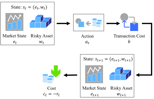
Figure 1: Illustration of the portfolio management problem.

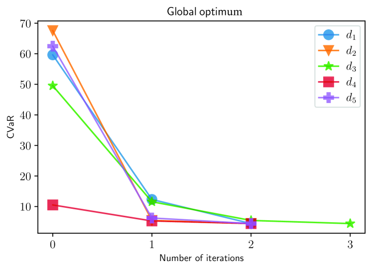
(a) The CVaR global optimum converged

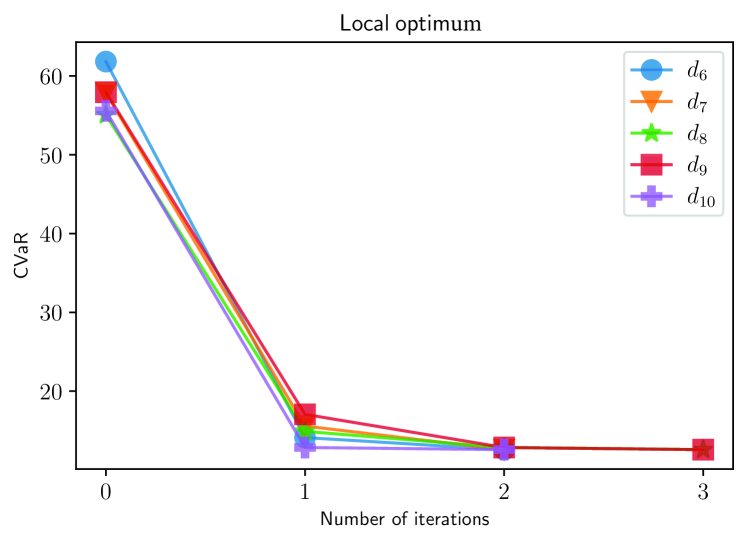
(b) The CVaR local optimum converged

Figure 2: The convergence procedure of Algorithm 1 under different initial policies. The last points on the curves are the convergence points.

We randomly select initial policies from the policy space and show the experimental result as example. From Figure 2, we observe that the value of CVaR decreases strictly in the iteration process until it converges. With different initial policies randomly chosen from the policy space, CVaR always converges to one of the two local optima, as shown in Figures 22(a)&2(b). For example, with initial policy $d_{1}$, the algorithm converges to the global optimum at the second iteration, and the associated CVaR is $4.43$. With initial policy $d_{6}$, the algorithm converges to the local optimum at the second iteration, and the associated CVaR is $12.58$. Given different initial policies, Algorithm 1 converges within two or three iterations in most cases, which demonstrates its fast convergence speed.

Moreover, we compare the distributions of system losses under the CVaR global optimal policy, the CVaR local optimal policy, and a random investment policy, which are illustrated with different colored histograms in Figure 3. The policy matrix of the CVaR global and local optimum is shown in Figure 44(a)&4(b), respectively. The random investment policy refers to a naive one choosing actions randomly at each state, which is illustrated by the policy matrix in Figure 44(c). Besides, we compute the long-run average optimal policy under which the mean of $c_{t}$ attains minimum, whose policy matrix is illustrated by Figure 44(d). From Figure 3, we can observe that the loss distribution under the CVaR global optimal policy has the minimal expected tail losses. The distribution of tail losses under the CVaR local optimal policy is also thinner than that of the random investment policy. In fact, the distribution of the CVaR global optimal policy is thinner than that of other policies. With the CVaR global policy shown in Figure 44(a), the investor should hold as few risky assets as possible in bear market and hold a little more risky assets in bull market. The mean optimal policy ignores the risk completely, and suggests the investor to hold as more risky assets as possible in any market state, even if there may be extreme losses. The performance comparison of mean, standard deviation, and CVaR under different policies are summarized in Table 3.

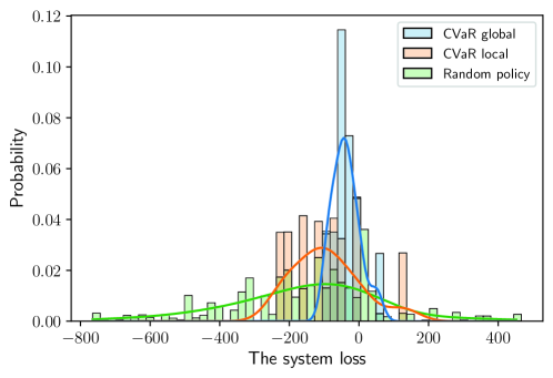
Figure 3: The distributions and fitting curves of the system losses under different policies.

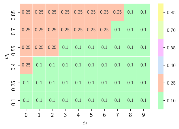
(a) The CVaR global optimal policy matrix

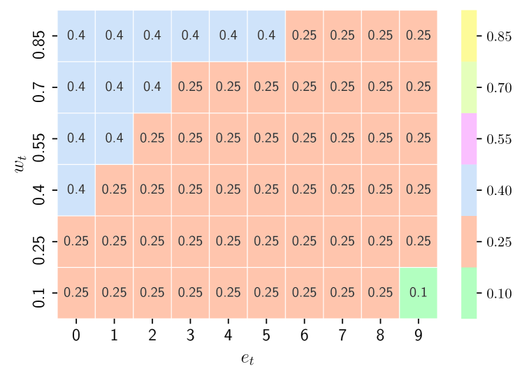
(b) The CVaR local optimal policy matrix

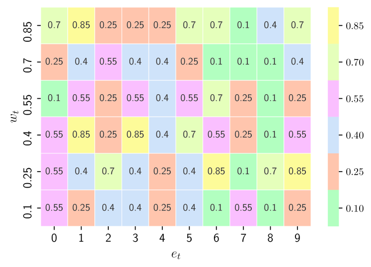
(c) The random policy matrix

(d) The mean optimal policy matrix

Figure 4: The policy matrices, where the horizontal axis represents the market condition, the vertical axis represents the percentage of the risky asset, and the number and color in the matrix represent the value of action $a_{t}\in\{0.1,0.25,0.4,0.55,0.7,0.85\}$.

Policy	$\eta(c_{t})$	$\sigma(c_{t})$	$\mathrm{CVaR}(c_{t})$
The CVaR global optimal policy	-37.55	37.91	4.43
The CVaR local optimal policy	-92.37	94.77	12.58
The random policy	-150.41	205.21	50.38
The mean optimal policy	-311.65	322.20	45.17

Table 3: Performance comparisons of different policies.

From the experiment results, we can see that our Algorithm 1 can optimize the CVaR metric effectively. The optimization algorithm has a fast convergence speed, which is analogous to the classical policy iteration algorithm. The local convergence of Algorithm 1 is also demonstrated.

5.2 Mean-CVaR Optimization of System Costs

In financial market, investors often need to control both the risk and the mean of losses in order to obtain stable returns. Thus, we conduct an experiment to demonstrate the mean-CVaR optimization discussed in Section 4.1. The optimization objective is $\mathrm{CVaR}(c_{t})+\beta\eta(c_{t})$. The probability level of $\mathrm{CVaR}$ is set as $\alpha=0.75$. All the other parameters are the same as those in the previous experiment. We first set $\beta=0.22$ and adapt Algorithm 1 to optimize the mean-CVaR combined objective. The convergence procedure is illustrated in Figure 5, where we can observe that the combined objective decreases strictly during the procedure and converges to $3.38$ at the third iteration.

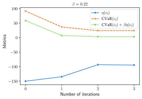
Figure 5: The convergence procedure of mean-CVaR optimization in portfolio management.

We also investigate the optimization results under different initial policies and different values of $\beta$. The convergence procedure is illustrated in Figure 6. For different values of $\beta$, we randomly choose 5 different initial policies to execute Algorithm 1. The convergence procedures under different initial policies are distinguished by different colored curves. There are two local optima when $\beta=0.4$, as shown in Figure 66. In other cases, different initial policies always converge to a single local optimum. The value of $\beta$ reflects the risk attitude of investors. For example, when $\beta=0.1$, it means that the investor is more risk averse and prefers to sacrifice potential returns to obtain a conservative investment policy. In contrast, when $\beta=2$, it indicates that the investor is more risk seeking and pursues more returns by buying more risky assets. Note that minimizing $\eta(c_{t})$ is equivalent to maximizing investment returns in this experiment. The corresponding optimal policies under different values of $\beta$ are shown in Figure 7, where we observe that the optimal policy becomes more risk seeking when the value of $\beta$ increases. Performance comparisons of different mean-CVaR optimal policies are summarized in Table 4. Numerical results demonstrate that Algorithm 1 can be extended to optimize both the mean and CVaR simultaneously, which is a common application scenario in finance.

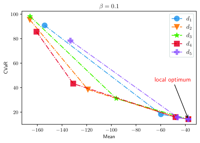
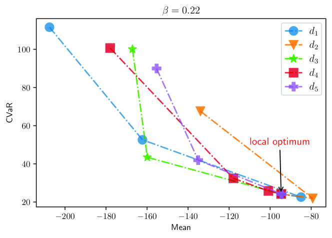
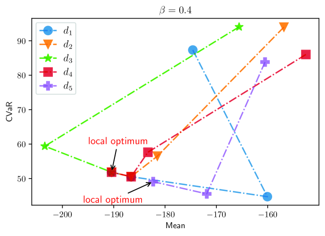
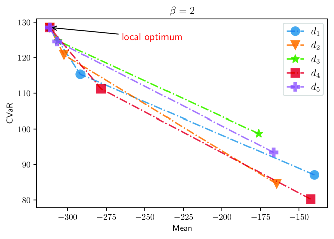
Figure 6: The convergence results under different values of $\beta$ and different initial policies.

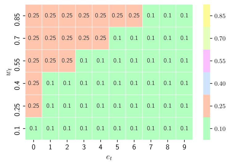
(a) The optimal policy when $\beta=0.1$

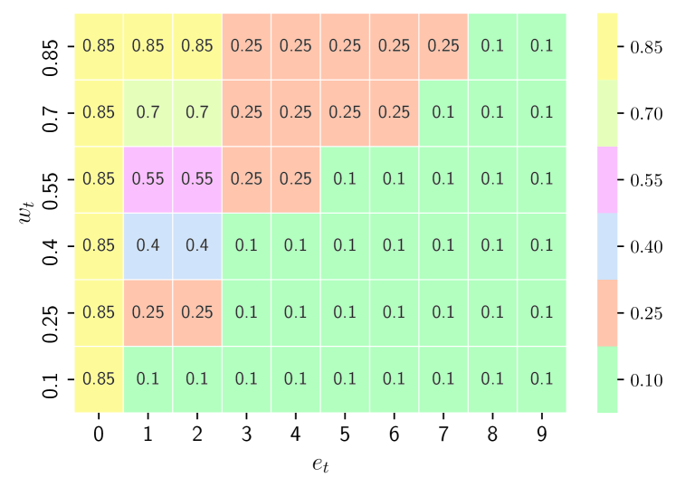
(b) The optimal policy when $\beta=0.22$

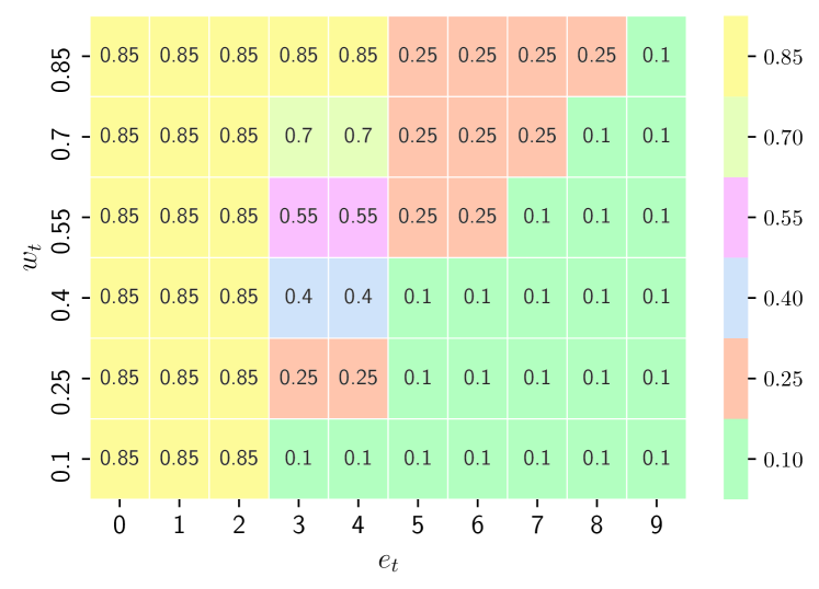
(c) The optimal policy when $\beta=0.4$

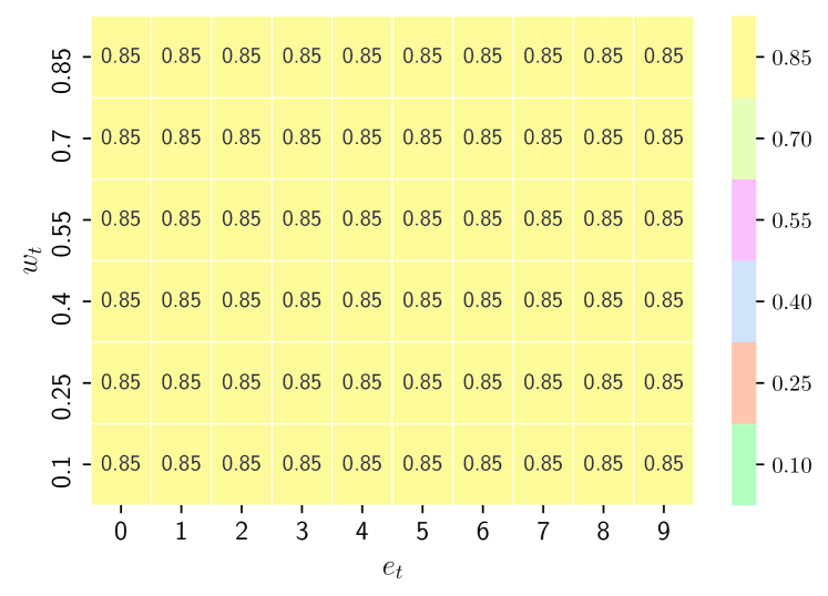
(d) The optimal policy when $\beta=2$

Figure 7: The mean-CVaR optimal policy matrices under different values of $\beta$.

Policy	$\mathrm{CVaR}(c_{t})$	$\eta(c_{t})$	$\mathrm{CVaR}(c_{t})+\beta\eta(c_{t})$
The optimal policy when $\beta=0.1$	14.24	-37.55	10.48
The optimal policy when $\beta=0.22$	24.20	-94.64	3.38
The global optimal policy when $\beta=0.4$	51.84	-190.42	-24.33
The local optimal policy when $\beta=0.4$	49.09	-182.31	-23.84
The optimal policy when $\beta=2$	128.52	-311.65	-494.77

Table 4: Performance comparisons of mean-CVaR optimal policies under different values of $\beta$.

6 Discussion and Conclusion

In this paper, we study the long-run CVaR optimization in the framework of MDPs. Because of the non-additive CVaR cost function, this dynamic optimization problem is not a standard MDP and traditional dynamic programming is not applicable. We study this problem by using sensitivity-based optimization. The long-run CVaR difference formula and derivative formula are both derived. Moreover, a so-called Bellman local optimality equation and other properties of optimal policies are obtained. With the CVaR sensitivity formulas, we further develop a policy iteration type algorithm to minimize long-run CVaR, and its local convergence is proved. Some possible extensions, including the mean-CVaR optimization and the long-run CVaR maximization, are also discussed.

Along with this research direction, it is valuable to further study other research topics. One topic is to extend the single objective of CVaR to multiple objectives, such as CVaR, mean, or their ratio metrics. Another topic is to extend our policy iteration type algorithm to other forms, such as value iteration or policy gradient type algorithms which are widely used in reinforcement learning. The combination with the techniques of sampling efficiency and neural network approximation for model-free scenarios is also a promising direction. It is expected that the Bellman local optimality equation and the CVaR sensitivity formulas will play important roles in the study of these topics.

Appendix

Proof of Lemma 4:

With the CVaR difference formula (23) for deterministic policy $d$ and mixed policy $d^{\delta,d^{\prime}}$, we can see that the derivative is written as below.

$$\frac{\partial\mathrm{CVaR}^{\delta}}{\partial\delta}\Big{|}_{\delta=0} = \lim\limits_{\delta\rightarrow 0}\frac{\mathrm{CVaR}^{\delta}-\mathrm{CVaR}^{d}}{\delta}$$ (34)

$$= \lim\limits_{\delta\rightarrow 0}\sum_{i\in\mathcal{S}}\pi^{\delta}(i)\Bigg{[}\sum_{j\in\mathcal{S}}[p(j|i,d^{\prime}(i))-p(j|i,d(i))]g^{d}(\mathrm{VaR}^{d},j)+\tilde{c}(\mathrm{VaR}^{d},i,d^{\prime}(i))$$

$$-\tilde{c}(\mathrm{VaR}^{d},i,d(i))\Bigg{]}+\lim\limits_{\delta\rightarrow 0}\frac{\Delta_{\mathrm{CVaR}}(\delta,d)}{\delta}$$

$$= \sum_{i\in\mathcal{S}}\pi^{d}(i)\Bigg{[}\sum_{j\in\mathcal{S}}[p(j|i,d^{\prime}(i))-p(j|i,d(i))]g^{d}(\mathrm{VaR}^{d},j)+\tilde{c}(\mathrm{VaR}^{d},i,d^{\prime}(i))$$

$$-\tilde{c}(\mathrm{VaR}^{d},i,d(i))\Bigg{]}+\lim\limits_{\delta\rightarrow 0}\frac{\Delta_{\mathrm{CVaR}}(\delta,d)}{\delta},$$

where we use the fact that $\lim\limits_{\delta\rightarrow 0}\pi^{\delta}(i)=\pi^{d}(i)$ since $d^{\delta,d^{\prime}}|_{\delta=0}=d$. Below, we study the last term in the above equation. From the definition (18), we have

$$\Delta_{\mathrm{CVaR}}(\delta,d)=\mathrm{CVaR}^{\delta}-\widetilde{\mathrm{CVaR}}^{\delta}(\mathrm{VaR}^{d})=\sum_{i\in\mathcal{S}}\sum_{a\in\mathcal{A}}\pi^{\delta}(i,a)[\tilde{c}(\mathrm{VaR}^{\delta},i,a)-\tilde{c}(\mathrm{VaR}^{d},i,a)].$$

Substituting (4) into the above equation, we have

$$\Delta_{\mathrm{CVaR}}(\delta,d)=\mathrm{VaR}^{\delta}-\mathrm{VaR}^{d}+\frac{1}{1-\alpha}\sum_{i\in\mathcal{S}}\sum_{a\in\mathcal{A}}\pi^{\delta}(i,a)\Big{\{}[c(i,a)-\mathrm{VaR}^{\delta}]^{+}-[c(i,a)-\mathrm{VaR}^{d}]^{+}\Big{\}}.$$ (35)

Without loss of generality, we assume $\mathrm{VaR}^{\delta}>\mathrm{VaR}^{d}$. We further define the following sets of state-action pairs

$$\begin{array}[]{lll}\mathcal{H}^{+}&:=&\{(i,a):c(i,a)\geq\mathrm{VaR}^{\delta}\},\\ \mathcal{H}_{-}&:=&\{(i,a):c(i,a)\leq\mathrm{VaR}^{d}\},\\ \mathcal{H}^{+}_{-}&:=&\{(i,a):\mathrm{VaR}^{d}<c(i,a)<\mathrm{VaR}^{\delta}\}.\end{array}$$ (36)

Substituting (36) into (35), we have

$$\Delta_{\mathrm{CVaR}}(\delta,d) = \mathrm{VaR}^{\delta}-\mathrm{VaR}^{d}+\frac{1}{1-\alpha}\Bigg{\{}\sum_{i,a\in\mathcal{H}^{+}}\pi^{\delta}(i,a)[c(i,a)-\mathrm{VaR}^{\delta}-c(i,a)+\mathrm{VaR}^{d}]$$ (37)

$$+\sum_{i,a\in\mathcal{H}^{+}_{-}}\pi^{\delta}(i,a)[\mathrm{VaR}^{\delta}-c(i,a)-c(i,a)+\mathrm{VaR}^{d}]+\sum_{i,a\in\mathcal{H}_{-}}\pi^{\delta}(i,a)[0-0]\Bigg{\}}$$

$$= \mathrm{VaR}^{\delta}-\mathrm{VaR}^{d}-\frac{\mathrm{VaR}^{\delta}-\mathrm{VaR}^{d}}{1-\alpha}\sum_{i,a\in\mathcal{H}^{+}}\pi^{\delta}(i,a)+\frac{1}{1-\alpha}\sum_{i,a\in\mathcal{H}^{+}_{-}}\pi^{\delta}(i,a)[\mathrm{VaR}^{\delta}$$

$$-2c(i,a)+\mathrm{VaR}^{d}]$$

$$= \frac{1}{1-\alpha}\sum_{i,a\in\mathcal{H}^{+}_{-}}\pi^{\delta}(i,a)[\mathrm{VaR}^{\delta}-2c(i,a)+\mathrm{VaR}^{d}],$$

where the last equality utilizes the fact that $\sum\limits_{i,a\in\mathcal{H}^{+}}\pi^{\delta}(i,a)=1-\alpha$. From (36), we can see that

$$\mathcal{H}^{+}_{-}\rightarrow\Phi,\qquad\mbox{when }\delta\rightarrow 0.$$ (38)

With the Mean Value Theorem, we also have

$$\mathrm{VaR}^{\delta}-2c(i,a)+\mathrm{VaR}^{d}\rightarrow 0,\qquad\mbox{when }\delta\rightarrow 0,\ (i,a)\in\mathcal{H}^{+}_{-}.$$ (39)

Substituting (38)&(39) into (37), we have

$$\frac{\partial\Delta_{\mathrm{CVaR}}(\delta,d)}{\partial\delta}\Big{|}_{\delta=0} = \frac{1}{1-\alpha}\Bigg{\{}\frac{\partial\mathrm{VaR}^{\delta}}{\partial\delta}\sum_{i,a\in\mathcal{H}^{+}_{-}}\pi^{\delta}(i,a)\Big{|}_{\delta=0}+\sum_{i,a\in\mathcal{H}^{+}_{-}}\frac{\partial\pi^{\delta}(i,a)}{\partial\delta}[\mathrm{VaR}^{\delta}-2c(i,a)+\mathrm{VaR}^{d}]\Big{|}_{\delta=0}\Bigg{\}}$$ (40)

$$= \frac{1}{1-\alpha}\Big{\{}0+0\Big{\}}=0.$$

Therefore, substituting the above equation (40) into (34), we directly have

$$\frac{\partial\mathrm{CVaR}^{\delta}}{\partial\delta}\Big{|}_{\delta=0}=\sum_{i\in\mathcal{S}}\pi^{d}(i)\Bigg{[}\sum_{j\in\mathcal{S}}[p(j|i,d^{\prime}(i))-p(j|i,d(i))]g^{d}(\mathrm{VaR}^{d},j)+\tilde{c}(\mathrm{VaR}^{d},i,d^{\prime}(i))-\tilde{c}(\mathrm{VaR}^{d},i,d(i))\Bigg{]}.$$

Then Lemma 4 is proved. ∎

References

- Aguirregabiria and Mira (2010) Aguirregabiria, V. and Mira, P. (2010). Dynamic discrete choice structural models: A survey. Journal of Econometrics 156(1), 38-67.
- Alexander et al. (2006) Alexander, S., Coleman, T. F., and Li, Y. (2006). Minimizing CVaR and VaR for portfolio of derivatives. J. Banking Finance 30, 583-605.
- Artzner et al. (1999) Artzner, P., Delbaen, F., Eber, J. M., Heath, D. (1999). Coherent measures of risk. Math. Finance 9, 203-228.
- Barron (2008) Barron, E. N. (2008). Game Theory: An Introduction. 2nd Edition. Wiley.
- Bäuerle and Ott (2011) Bäuerle, N. and Ott J. (2011). Markov decision processes with average-value-at-risk criteria. Mathematical Methods of Operations Research 74(3), 361-379.
- Bertsekas (2005) Bertsekas, D. P. (2005). Dynamic Programming and Optimal Control–Vol. I. Athena Scientific.
- Boda and Filar (2006) Boda, K. and Filar, J. (2006). Time consistent dynamic risk measures. Math Methods Oper Res 63, 169-186.
- Cao (2007) Cao, X. R. (2007). Stochastic Learning and Optimization – A Sensitivity-Based Approach. New York: Springer.
- Chung (1994) Chung, K. J. (1994). Mean-variance tradeoffs in an undiscounted MDP: the unichain case. Operations Research 42, 184-188.
- Feinberg and Shwartz (2002) Feinberg, E. A. and Shwartz, A. (eds.) (2002). Handbook of Markov Decision Processes: Methods and Applications. Kluwer, Boston.
- Fu et al. (2009) Fu, M. C., Hong, L. J., and Hu, J. Q. (2009). Conditional Monte Carlo estimation of quantile sensitivities. Management Science 55 (12), 2019-2027.
- Haskell and Jain (2015) Haskell, W. B. and Jain, R. (2015). A convex analytic approach to risk-aware Markov decision processes. SIAM Journal on Control and Optimization 53(3), 1569-1598.
- Hong et al. (2014) Hong, L. J., Hu, Z., and Liu, G. (2014). Monte Carlo methods for value-at-risk and conditional value-at-risk: A review. ACM Transactions on Modeling and Computer Simulation 24, 1-37.
- Huang and Guo (2016) Huang, Y. and Guo, X. (2016). Minimum average value-at-risk for finite horizon semi-Markov decision processes in continuous time. SIAM Journal on Optimization 26(1), 1-28.
- Kaelbling et al. (1996) Kaelbling, L. P., Littman, M. L., and Moore, A. W. (1996). Reinforcement learning: A survey. Journal of Artificial Intelligence 4, 237-285.
- Lewis et al. (2012) Lewis, F.L., Vrabie, D.L. and Syrmos, V.L. (2012). Optimal Control, 3rd Edition. John Wiley & Sons, Hoboken.
- Littman (1994) Littman, M. L. (1994). Markov games as a framework for multi-agent reinforcement learning. Machine Learning Proceedings 1994, 157-163. Morgan Kaufmann.
- Markowitz (1952) Markowitz, H. (1952). Portfolio selection. The Journal of Finance 7, 77-91.
- Miller and Yang (2017) Miller, C. W. and Yang, I. (2017). Optimal control of conditional value-at-risk in continuous time. SIAM Journal on Control and Optimization 55(2), 856-884.
- Pflug and Pichler (2016) Pflug, G. C. and Pichler, A. (2016). Time-consistent decisions and temporal decomposition of coherent risk functionals. Mathematics of Operations Research 41(2), 682-699.
- Puterman (1994) Puterman, M. L. (1994). Markov Decision Processes: Discrete Stochastic Dynamic Programming. New York: John Wiley & Sons.
- Rockafellar and Uryasev (2000) Rockafellar, R. T. and Uryasev, S. (2000). Optimization of conditional value-at-risk. Journal of Risk 2(3), 21-42.
- Rockafellar and Uryasev (2002) Rockafellar, R. T. and Uryasev, S. (2002). Conditional Value-at-Risk for general loss distributions. Journal of Banking Finance 26, 1443-1471.
- Rust (1987) Rust, J. (1987). Optimal replacement of GMC bus engines: An empirical model of Harold Zurcher. Econometrica 55, 999-1033.
- Sobel (1994) Sobel, M. J. (1994). Mean-variance tradeoffs in an undiscounted MDP. Operations Research 42, 175-183.
- Sutton and Barto (2018) Sutton, R. S. and Barto, A. G. (2018). Reinforcement Learning: An Introduction, 2nd Edition. MIT Press, Cambridge, MA.
- Xia (2020) Xia, L. (2020). Risk-sensitive Markov decision processes with combined metrics of mean and variance. Production and Operations Management 29(12), 2808-2827.
- Xia et al. (2014) Xia, L., Jia, Q. S., and Cao, X. R. (2014). A tutorial on event-based optimization – A new optimization framework. Discrete Event Dynamic Systems: Theory and Applications 24(2), 103-132.
- Uǧurlu (2017) Uǧurlu, K. (2017). Controlled Markov decision processes with AVaR criteria for unbounded costs. Journal of Computational and Applied Mathematics 319, 24-37.
- von Neumann (1928) Von Neumann, J. (1928). Zur Theorie der Gesellschaftsspiele. Mathematische Annalen 100, 295-320. doi:10.1007/BF01448847.
- Zhou et al. (2022) Zhou, Z., Athey, S., and Wager, S. (2022). Offline multi-action policy learning: Generalization and optimization. Operations Research, arXiv:1810.04778.