Towards a theory of surface orbital magnetization

Abstract

The theory of bulk orbital magnetization has been formulated both in reciprocal space based on Berry curvature and related quantities, and in real space in terms of the spatial average of a quantum mechanical local marker. Here we consider a three-dimensional antiferromagnetic material having a vanishing bulk but a nonzero surface orbital magnetization. We ask whether the surface-normal component of the surface magnetization is well defined, and if so, how to compute it. As the physical observable corresponding to this quantity, we identify the macroscopic current running along a hinge shared by two facets. However, the hinge current only constrains the difference of the surface magnetizations on the adjoined facets, leaving a potential ambiguity. By performing a symmetry analysis, we find that only crystals exhibiting a pseudoscalar symmetry admit well-defined magnetizations at their surfaces at the classical level. We then explore the possibility of computing surface magnetization via a coarse-graining procedure applied to a quantum local marker. We show that multiple expressions for the local marker exist, and apply constraints to filter out potentially meaningful candidates. Using several tight-binding models as our theoretical test bed and several potential markers, we compute surface magnetizations for slab geometries and compare their predictions with explicit calculations of the macroscopic hinge currents of rod geometries. We find that only a particular form of the marker consistently predicts the correct hinge currents.

I Introduction

The modern theories of bulk electric polarization P and bulk orbital magnetization M King-Smith and Vanderbilt (1993); Vanderbilt and King-Smith (1993); Xiao et al. (2005); Thonhauser et al. (2005); Ceresoli et al. (2006); Shi et al. (2007); Souza and Vanderbilt (2008) express these quantities as Brillouin zone integrals of quantities involving Berry connections and curvatures of ground state Bloch functions. However, the ground-state of systems of independent electrons may also be uniquely described by the single-particle density matrix, also known as the ground state projector $P(\textbf{r},\textbf{r}^{\prime})$. This is a quantity that for insulating states of matter decays exponentially with $|\textbf{r}-\textbf{r}^{\prime}|$, even for Chern insulators Thonhauser and Vanderbilt (2006).

A natural question to ask is whether it is possible to express P and M in terms of $P(\textbf{r},\textbf{r}^{\prime})$. In the case of the polarization, while the change $\Delta\textbf{P}$ can be determined by following the change of $P(\textbf{r},\textbf{r}^{\prime})$ between two states connected by an adiabatic switching process, there is no corresponding expression for P itself, which is determined only modulo a quantum King-Smith and Vanderbilt (1993); Vanderbilt and King-Smith (1993).

However, M does not suffer from any quantum of indeterminacy, and should be expressible via the ground state projector. Bianco and Resta Bianco and Resta (2013) demonstrated that this is, in fact, correct. Starting from an expression for a simple 2D crystallite of finite area, the authors demonstrated that for any insulator, even a Chern insulator, the orbital magnetization $M$ is given in the thermodynamic limit by

$$M=\frac{1}{A}\int_{A}\mathcal{M}(\textbf{r})d\textbf{r}.$$ (1)

Here $A$ is the bulk unit cell area and $\mathcal{M}(\textbf{r})$ is a local function, hereafter referred to as the local marker, which is expressed in terms of $P(\textbf{r},\textbf{r}^{\prime})$. For large finite samples in the thermodynamic limit, the averaging in Eq. (1) may equivalently be performed over the entire crystallite. Although $\mathcal{M}(\textbf{r})$ appears to play the role of magnetic dipole density, only it’s macroscopic average bears any physical meaning. This is in keeping with the fact that while microscopic charge and current densities are well defined, microscopic dipole densities (be it charge or orbital magnetic) are not Hirst (1997).

Recent years have witnessed numerous efforts aimed at defining and providing explicit expressions for surface-specific analogues of bulk quantities. Examples include the surface anomalous Hall conductivity (AHC) Rauch et al. (2018); Varnava et al. (2020) and the surface-parallel boundary electric polarization Zhou et al. (2015); Benalcazar et al. (2017a, b); Ren et al. (2021); Trifunovic (2020) on the surface of a bulk insulator. To date, however, there has been very little discussion of surface orbital magnetization in the literature Zhu et al. (2021); Bianco and Resta (2016), and a complete theory of orbital magnetization at the surface of a bulk material has yet to be developed.

In the present work, we explore the possibility of defining surface orbital magnetization. By this we mean the excess surface-normal macroscopic magnetization (magnetic moment per unit area) at the surface of a bulk material with broken time-reversal (TR) symmetry. Our investigation is restricted to antiferromagnetic systems featuring a vanishing bulk magnetization, as this allows us to readily disentangle surface contributions to the orbital magnetization from those stemming from the bulk. We shall also restrict ourselves throughout to the case of insulating surfaces of insulating crystals, leaving aside for now any special considerations that might arise for metallic surfaces.

The case of surface spin magnetization is much more straightforward, as the latter can be obtained simply by integrating the net spin density $\Delta n=n_{\uparrow}-n_{\downarrow}$ over the surface region after an appropriate coarse-graining (e.g., using window-averaging methods). In the remainder of this work, therefore, we focus solely on the orbital component of the surface magnetization. Here it is natural to expect more difficulties, since even the theory of bulk orbital magnetization has been put on a solid footing only in relatively recent times Xiao et al. (2005); Thonhauser et al. (2005); Ceresoli et al. (2006); Shi et al. (2007); Souza and Vanderbilt (2008). The essential problem, as in the theory of electric polarization, is that the position operator is ill defined in the Bloch representation, so that methods based on Berry connections and curvatures are required instead. Another way to frame the problem is to note that quantum-mechanical expressions are available for neither the local polarization density $\mathbf{P}(\mathbf{r})$ nor the local orbital magnetization density $\mathbf{M}(\mathbf{r})$.

Even at a classical level, another difficulty arises. Recall that, while the bulk orbital magnetization cannot be inferred from the local current distribution deep in the bulk, it can be deduced with the added knowledge of the currents on its surface facets. By analogy, one might expect that the surface magnetization on a given facet can be inferred in a similar way from the added knowledge of the currents flowing at the edges of the facet. However, such a facet boundary is always a hinge where two facets meet, with the hinge current given by the difference between the surface magnetizations on the two adjoining facets. Since the hinge currents only determine surface magnetization differences, this raises the question whether surface orbital magnetization can be uniquely determined, or only determined up to a constant shift in the values predicted for all facets, even when given a perfect knowledge of all local currents. Such a “shift freedom” is an unavoidable feature of a classical description starting from current densities, and is related to the fact that while the curl of $\mathbf{M}(\mathbf{r})$ is constrained by the current distribution, its divergence is not.

With the introduction of a quantum description, the bulk electric polarization and orbital magnetization, which were ill determined from a classical knowledge of bulk charge and current densities, become well defined based on a knowledge of the bulk Bloch eigenstates (up to a quantum in the case of the polarization). In a similar way, one might hope that an appropriate quantum description of the surface problem would allow for a robust prescription for computing surface orbital magnetization from a knowledge of surface, as well as bulk, ground state wave functions. This is the goal of the present work.

In this paper, we first investigate the role of symmetry and show that certain classes of symmetries do allow for the surface magnetization to be uniquely extracted from a knowledge of hinge currents, even at the classical level. We then turn to the quantum problem and explore whether the use of a local marker $\mathcal{M}(\textbf{r})$, such as the one proposed by Bianco and Resta, can be adopted for the purpose of defining a surface orbital magnetization. That is, even if the value of $\mathcal{M}(\textbf{r})$ at a single point has no obvious physical meaning, we ask whether it is possible to coarse-grain and integrate such a marker over the surface region to obtain a valid expression for the surface orbital magnetization.

This paper is organized as follows. In Sec. II, we identify the physical observable corresponding to the presence of a surface magnetization, namely the macroscopic current running along a hinge shared by adjacent surface facets of a bulk crystal, given by the difference between the magnetizations of the two surface facets forming the hinge. We show that within the framework of a classical theory, this single relation is insufficient to ascribe a uniquely defined value of magnetization to any of the facets; constraints in the form of crystalline symmetries are required to accomplish this. In Sec. III, we identify all the possible symmetries that lead to unambiguous surface magnetizations. We find that this set of symmetries is identical to the set of symmetries that quantizes the Chern-Simons axion coupling.

In Sec. IV we introduce in greater detail the local marker formulation of orbital magnetism, and introduce our formalism for the calculation of surface magnetization and hinge currents. The results of Sec. III and Sec. IV are later tested in Sec. V by calculations performed on tight-binding models. We end our paper with a discussion of our results and some speculations on their connection to the theory of orbital magnetic quadrupole moments in Sec. VI, and summarize in Sec. VII.

II Surface Magnetizations and Hinge Currents

Consider a stand-alone 2D system such as a monolayer or multilayer with layer-normal magnetization $M_{\perp}$. The magnetization manifests itself on any edge of the system as a macroscopic bound current of magnitude $M_{\perp}$, with its sign determined from the right-hand rule. At the classical level, $M_{\perp}$ can be determined from the combined knowledge of the microscopic current density deep in the bulk and at the edge. Without the added knowledge of the current density at the edge, however, $M_{\perp}$ can be determined only from a knowledge of the quantum-mechanical bulk Bloch eigenstates.

If instead we consider the surface of a 3D bulk system (with vanishing bulk magnetization), we would also expect any surface-normal magnetization at the surface to manifest itself at an edge in a similar fashion. However, in the presence of the bulk, the objects playing the role of edges are the hinges, i.e., the intersections of neighboring surface facets. So, while in the case of an isolated 2D system the edge current directly determines the magnetization $M_{\perp}$, any current present on a hinge only determines the difference of $M_{\perp}$ values on the two surface facets meeting at the hinge. Hence a classical knowledge of the microscopic current distribution in the bulk, at the surfaces, and at the hinge is sufficient to uniquely determine the difference of $M_{\perp}$ values across facets sharing a hinge, but not the $M_{\perp}$ values individually. We depict this situation schematically in Fig. 1, where it is evident that

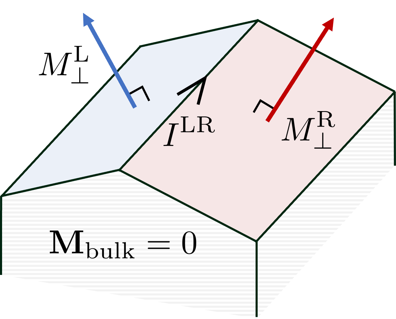
Figure 1: Schematic depicting a hinge and the surface facets that compose it. The black arrowhead on the hinge depicts the direction of flow for the hinge current $I^{\text{LR}}$ to be positive. The maroon and blue arrows denote the surface-normal magnetization vectors $M^{\text{R}}_{\perp}$ and $M^{\text{L}}_{\perp}$, respectively. The hinge current is $I^{\text{LR}}=M^{\text{L}}_{\perp}-M^{\text{R}}_{\perp}$.

the hinge current $I^{\text{LR}}$ is given by

$$I^{\text{LR}}=M^{\text{L}}_{\perp}-M^{\text{R}}_{\perp}.$$ (2)

Note that a line current may also be present at a line defect, such as a step or domain wall Varnava et al. (2021), that separates surface patches having the same orientation but different $M_{\perp}$ values. We can regard these as 180^∘ hinges, and the treatment of such cases introduces no new difficulties. In the remainder of this work, we restrict the discussion to true hinges connecting facets of different orientation. In any case, we emphasize that the line currents in question are bound currents localized at insulating hinges, not the chiral conductance channels that may occur in topological systems, e.g., at the boundary of a 2D quantum Hall state or on the hinges of an axion insulator Khalaf (2018); Varnava and Vanderbilt (2018).

For the entirety of this paper, we take the hinge current to be a physical observable, being detectable in principle by the circulating magnetic field it creates. Combined with Eq. (2), this assumption indicates that differences between magnetizations on neighboring surface facets are also observables, in addition to being classically well defined in the sense described earlier. However, there is no a priori reason to believe that the individual values of facet magnetizations are either observables or are uniquely defined in the context of classical theory.

As mentioned in the Introduction and explicitly demonstrated by Eq. (2), the individual values of the facet magnetizations are defined classically only up to a common constant shift, resulting in a shift freedom. To understand how the shift freedom arises, consider a finite crystallite embedded in vacuum. The crystallite’s steady state microscopic current density $\textbf{j}(\textbf{r})$ is divergenceless, and thus may be expressed as the curl of a vector field $\textbf{M}(\textbf{r})$ with the interpretation of a local magnetization density. However, $\textbf{M}(\textbf{r})$ has a “gauge freedom” in that augmenting $\textbf{M}(\textbf{r})$ by the gradient of an arbitrary scalar field $f(\textbf{r})$ leaves $\textbf{j}(\textbf{r})$ unchanged. In particular, let $f(\textbf{r})$ be some function that is periodic with average value $\Delta$ in the interior, vanishes in the vacuum region outside, and transitions from these behaviors over a few lattice constants at the surface. Then at the coarse-grained level, the new $\textbf{M}(\textbf{r})$ differs from the old one by what appears to be a delta-function concentration of $M_{\perp}$ of magnitude $-\Delta$ on all surface facets. This is precisely the shift freedom.

We must therefore understand whether, or under what circumstances, we can resolve this ambiguity and assign a unique $M_{\perp}$ to a given facet of the bulk. Once an unambiguous value of magnetization is assigned to even a single facet, we may then repeatedly employ Eq. (2) to find the magnetization at any other facet of the 3D crystallite.

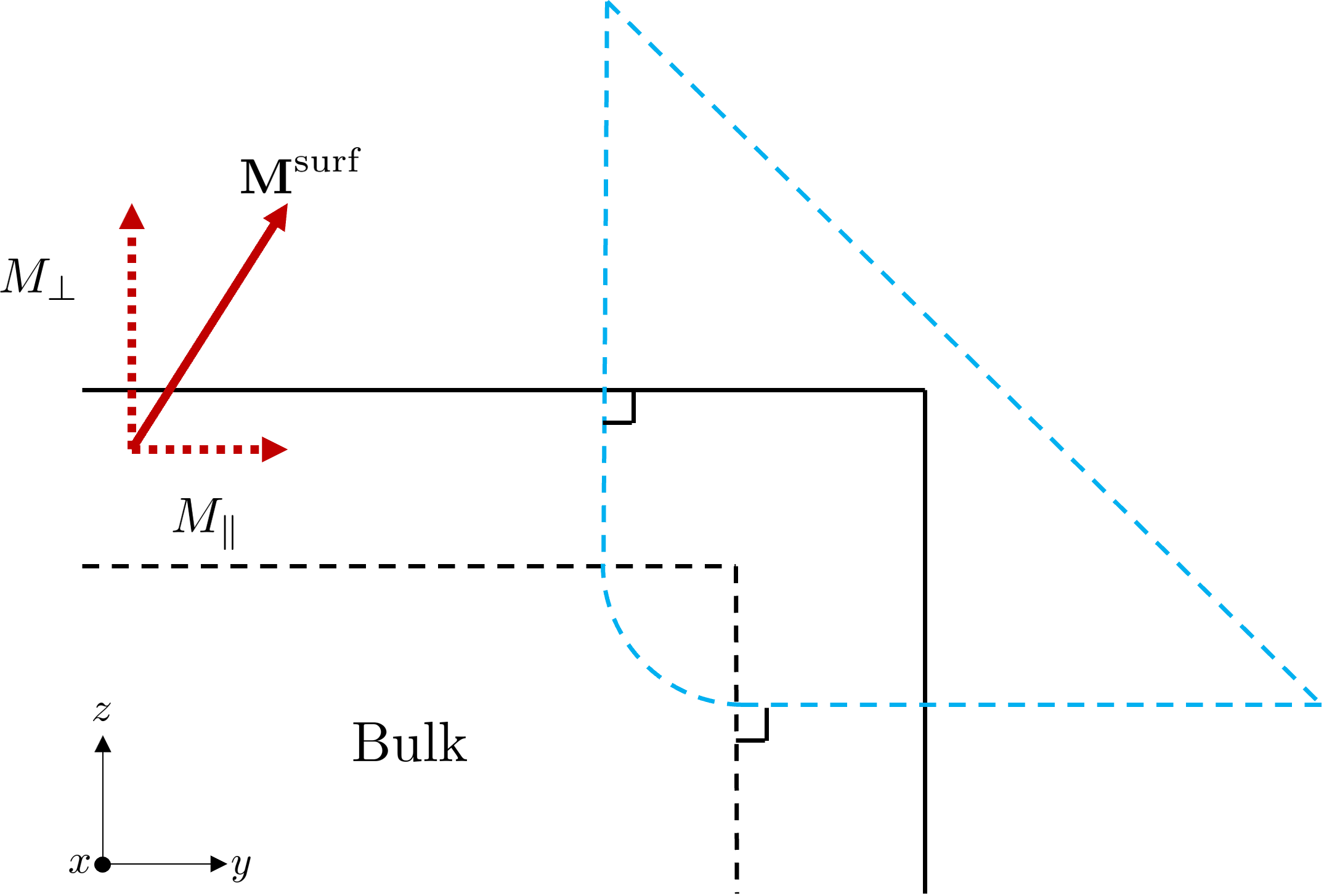
Figure 2: Schematic depiction of a hinge formed by two surface facets, one of which has a magnetization $\textbf{M}^{\text{surf}}$ that is not normal to the surface, having components $M_{\perp}$ along $\hat{\textbf{z}}$ and $M_{\parallel}$ along $\hat{\textbf{y}}$. $M_{\parallel}$ is observable in principle by the presence of a concentration of magnetic field $B_{y}$ in the surface region. The hinge current is observable via the integral $\oint\textbf{M}\cdot d\textbf{l}$ around the dashed blue Amperian loop, which remains normal to the surface while passing through the surface region delineated by the dashed black line.

While we have focused above on the surface-normal component of the surface orbital magnetization, an in-plane component $M_{\parallel}$ could also be present. If so, its strength is easily computed from a detailed knowledge of the microscopic current distribution in the surface region, unlike the more problematic $M_{\perp}$. In principle, $M_{\parallel}$ should be observable by the presence of a corresponding concentration of $B_{\parallel}$ in the surface region (since H vanishes in this geometry in the absence of free current). When $M_{\parallel}$ is present, we can filter out its contribution to the hinge current by constructing an appropriate Amperian loop that is normal to both surface facets, as depicted in Fig. 2. Integrating the magnetization around this loop yields the bound current passing through the loop. Since we assume the absence of free current, and since the vacuum and bulk are free of magnetization, only the top and side $M_{\perp}$ values contribute to the hinge current. We adopt this as the definition of the hinge current in such situations.

III Symmetries and Surface Magnetization

The goal of this section is to establish under what circumstances we can specify a uniquely defined magnetization on a given surface facet of a 3D crystallite in the context of classical theory. By this, we mean whether a classical knowledge of the microscopic current distribution in the bulk, at the surfaces, and at the hinges is sufficient to assign a unique value of $M_{\perp}$ to a given surface facet. As noted in the previous section, Eq. (2) effectively results in one equation in two unknowns, which prevents an assignment of definite values to $M^{\text{L}}_{\perp}$ and $M^{\text{R}}_{\perp}$. We therefore need additional restrictions on the possible values $M^{\text{L}}_{\perp}$ and $M^{\text{R}}_{\perp}$ may take. In this Section, these restrictions will appear in the form of symmetry-induced constraints. We first introduce the notation we will be using to describe the actions of the symmetry operations, and subsequently delve into the symmetry analysis of surface magnetization.

	$M_{\perp}$-preserving	$M_{\perp}$-reversing
$\hat{\textbf{n}}$-reversing	$R^{+}_{\hat{\textbf{n}}}$	$R^{-}_{\hat{\textbf{n}}}$
$\hat{\textbf{n}}$-symmorphic	$S^{+}_{\hat{\textbf{n}}}$	$S^{-}_{\hat{\textbf{n}}}$
$\hat{\textbf{n}}$-nonsymmorphic	$N^{+}_{\hat{\textbf{n}}}$	$N^{-}_{\hat{\textbf{n}}}$

Table 1: Summary of labels attached to a symmetry operation depending on whether it reverses $\hat{\textbf{n}}$ ($R$) or not ($S,N$), where $S$ and $N$ refer to $\hat{\textbf{n}}$-symmorphic and $\hat{\textbf{n}}$-nonsymmorphic operations respectively. Superscripts ‘$-$’ and ‘$+$’ indicate whether or not the operation reverses the sign of the outward-directed $M_{\perp}$ on a surface with normal $\hat{\textbf{n}}$, which also corresponds to whether the symmetry operation is axion-odd or axion-even.

III.1 Notation

Consider a surface with unit normal $\hat{\textbf{n}}$. Let the outward surface-normal component of the surface magnetization be $M_{\perp}=\textbf{M}\cdot\hat{\textbf{n}}$, with units of magnetic moment per unit area. With respect to this choice of $\hat{\textbf{n}}$, we will focus on operations that either preserve or reverse the direction $\hat{\textbf{n}}$, as well as those that preserve or flip the sign of $M_{\perp}$. Operations that flip $\hat{\textbf{n}}$ will be denoted by $R^{\pm}_{\hat{\textbf{n}}}$; the superscript ‘$+$’ or ‘$-$’ indicates that $M_{\perp}$ is preserved or flipped, respectively. We further classify operations that preserve $\hat{\textbf{n}}$ as either symmorphic or nonsymmorphic along that direction, where by the latter term we mean operations that involve a fractional translation along $\hat{\textbf{n}}$, such as a screw or glide mirror operation. Thus, $\hat{\textbf{n}}$-symmorphic operations will be denoted $S^{\pm}_{\hat{\textbf{n}}}$ (even if they involve fractional translations in the plane normal to $\hat{\textbf{n}}$), while $\hat{\textbf{n}}$-nonsymmorphic operations will be denoted $N^{\pm}_{\hat{\textbf{n}}}$.

We summarize the classification of symmetries in Table 1. We note that operations labeled with a superscript ‘$-$’ are axion-odd while those labeled with a ‘$+$’ superscript are axion-even. By definition, an axion-odd symmetry is either a proper spatial rotation with time reversal or an improper rotation without time reversal. The significance of this distinction will become clear in Sec. III.3.

For concreteness, let $\hat{\textbf{n}}=\hat{\textbf{z}}$. We list all the symmetry operations that fall into the categories listed above in Table 2. In our notation, $E$ denotes the identity operation and $I$ denotes inversion. $C_{n}$ denotes a rotation by $2\pi/n$ about the $\hat{\textbf{z}}$ axis ($n=2,3,4,6$) while $\overline{C}_{2}$ is a 2-fold rotation about an axis in the $x$-$y$ plane. $m_{z}$ denotes a mirror reflection across the $x$-$y$ plane, and $m_{d}$ is a mirror reflection across a plane containing the $\hat{\textbf{z}}$ axis. $S_{n}=m_{z}C_{n}$ denotes an improper rotation (rotoinversion) about the $\hat{\textbf{z}}$ axis. A prime indicates composition with time reversal. Nonsymmorphic fractional translations along $\hat{\textbf{z}}$ are indicated as $c/2$ or $pc/n$, where $c$ is the vertical lattice constant and $p<n$ is an integer (or half-integer in the case of $C^{\prime}_{3}$). Half lattice translations in the $x$-$y$ plane are indicated by $\bm{\tau}_{d/2}$. In what follows, we shall often denote the screw operation $\{C_{n}|pc/n\}$ as just $n_{p}$ for conciseness.

It is important to note that some of the above operations may belong to $R$, $S$, and $N$ operations with respect to other directions. For example, the glide mirror $\{m_{y}|c/2\}$ is both an $N^{-}_{\hat{\textbf{z}}}$ and an $R^{-}_{\hat{\textbf{y}}}$ operation.

Type	Symmetry Operations
$R^{-}_{\hat{\textbf{z}}}$	$m_{z}$, $I$, $S_{3,4,6}$, $\overline{C}^{\prime}_{2}$, $\{m_{z}|\bm{\tau}_{d/2}\}$, $\{\overline{C}^{\prime}_{2}|\bm{\tau}_{d/2}\}$
$S^{-}_{\hat{\textbf{z}}}$	$E^{\prime}$, $\{E^{\prime}|\bm{\tau}_{d/2}\}$, $C^{\prime}_{n}$, $m_{d}$
$N^{-}_{\hat{\textbf{z}}}$	$\{E^{\prime}|c/2\}$, $\{C^{\prime}_{n}|pc/n\}$, $\{m_{d}|c/2\}$
$R^{+}_{\hat{\textbf{z}}}$	$m^{\prime}_{z}$, $I^{\prime}$, $S^{\prime}_{3,4,6}$, $\overline{C}_{2}$, $\{m^{\prime}_{z}|\bm{\tau}_{d/2}\}$, $\{\overline{C}_{2}|\bm{\tau}_{d/2}\}$
$S^{+}_{\hat{\textbf{z}}}$	$C_{n}$, $m^{\prime}_{d}$
$N^{+}_{\hat{\textbf{z}}}$	$\{C_{n}|pc/n\}$, $\{m^{\prime}_{d}|c/2\}$

Table 2: List of all the specific symmetry operations that belong to each symmetry operation type.

III.2 Symmetry Analysis for Surface Magnetization

In this subsection, we explore how to exploit the symmetry operations in the $S^{\pm}_{\hat{\textbf{n}}}$, $R^{\pm}_{\hat{\textbf{n}}}$, and $N^{\pm}_{\hat{\textbf{n}}}$ classes to define an unambiguous surface magnetization on at least one surface facet; repeated application of Eq. (2) will subsequently help define magnetizations for all other surface facets. The main idea is that a given symmetry operation will relate specific surface facets to one another, allowing us to explicitly relate physical quantities defined on those facets. We then consider the magnetizations $M_{\perp}$ at the surfaces, and check whether this configuration allows for an unambiguous determination of these $M_{\perp}$ values. We find that $S^{-}_{\hat{\textbf{n}}}$, $R^{-}_{\hat{\textbf{n}}}$, and $N^{-}_{\hat{\textbf{n}}}$ operations allow us to define unambiguous surface magnetizations, while for $S^{+}_{\hat{\textbf{n}}}$, $R^{+}_{\hat{\textbf{n}}}$, and $N^{+}_{\hat{\textbf{n}}}$ this is not possible.

As a reminder, we are focusing on $\hat{\textbf{n}}=\hat{\textbf{z}}$ for concreteness. We first investigate the axion-odd symmetries $S^{-}_{\hat{\textbf{z}}}$, $R^{-}_{\hat{\textbf{z}}}$, and $N^{-}_{\hat{\textbf{z}}}$, and subsequently the axion-even symmetries $S^{+}_{\hat{\textbf{z}}}$, $R^{+}_{\hat{\textbf{z}}}$, and $N^{+}_{\hat{\textbf{z}}}$.

Symmetries of type $S^{-}_{\hat{\textbf{z}}}$.

Suppose we find a symmetry of the type $S^{-}_{\hat{\textbf{z}}}$ in the bulk symmetry group. We may then construct a surface respecting this symmetry with unit normal $\hat{\textbf{z}}$. Under an $S^{-}_{\hat{\textbf{z}}}$ operation, the surface will remain invariant, but the magnetization at the surface will be flipped. This can only mean that the magnetization at the surface is zero.

Symmetries of type $R^{-}_{\hat{\textbf{z}}}$.

If we find an $R^{-}_{\hat{\textbf{z}}}$ symmetry in the bulk symmetry group, we may construct a finite slab in $z$ consistent with the identified $R^{-}_{\hat{\textbf{z}}}$ symmetry applied to the slab as a whole. This construction will then enforce identical magnetizations on top and bottom surfaces.

Let us introduce an arbitrary third surface facet to the slab, as shown in Fig. 3. In the figure, the arrows normal to the surfaces indicate the direction of the surface-normal magnetization in the given global Cartesian frame. The vectors are labeled by their corresponding magnitudes; since $M^{\text{B}}_{\perp}<0$, the magnitude of the bottom surface magnetization is labeled as $-M^{\text{B}}_{\perp}$. We then also have two hinges with currents $I_{1}$ and $I_{2}$, with the directions of the arrowheads on the hinges indicating the directions of positive current flow.

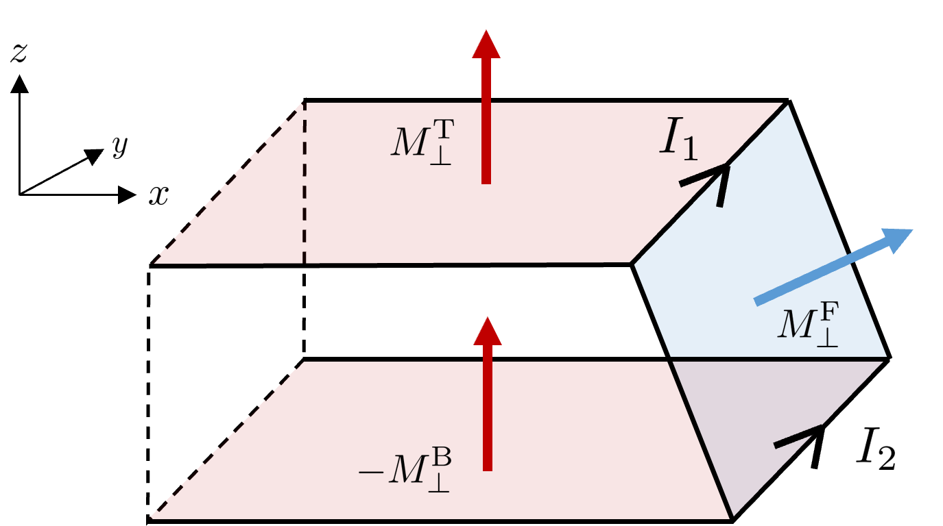
Figure 3: Schematic of a slab geometry for a bulk material with an $R^{-}_{\hat{\textbf{z}}}$ symmetry. An additional facet of arbitrary orientation appears at right. The $R^{-}_{\hat{\textbf{z}}}$ symmetry ensures that the magnetizations on the top and bottom facets are equal and parallel, as indicated by the maroon arrows. All three facet magnetizations may be found using the known hinge currents $I_{1}$ and $I_{2}$, as discussed in the text.

Using our knowledge of these currents and the symmetry of the bulk slab, we may then write down a system of equations

$$0 =M^{\text{T}}_{\perp}+M^{\text{B}}_{\perp},$$

$$I_{1} =M^{\text{T}}_{\perp}-M^{\text{F}}_{\perp},$$ (3)

$$I_{2} =M^{\text{F}}_{\perp}-M^{\text{B}}_{\perp},$$

that can be solved for the three facet magnetizations.

Symmetries of type $N^{-}_{\hat{\textbf{z}}}$.

From Table 2 we see that there are three types of operations belonging to the $N^{-}_{\hat{\textbf{z}}}$ class: the time reversed half-translation $\{E^{\prime}|c/2\}$, glide mirrors $\{m_{d}|c/2\}$, and time reversed screw symmetries. Note that $\{E^{\prime}|c/2\}$ is also a $S^{-}_{\hat{\textbf{d}}}$ operation, while $\{m_{d}|c/2\}$ and $\{C^{\prime}_{2z}|c/2\}$ are also $R^{-}_{\hat{\textbf{d}}}$ operations. We therefore already know that we can define unambiguous surface magnetizations in those cases. We thus focus on the time-reversed screws with 3-fold, 4-fold, and 6-fold rotation axes.

For these operations, we construct crystallites in the shape of regular triangular, square, or hexagonal prisms, respectively, as shown schematically in Fig. 4. Each prism is infinite along $z$ and is constructed to respect the corresponding screw symmetry applied to the rod as a whole.

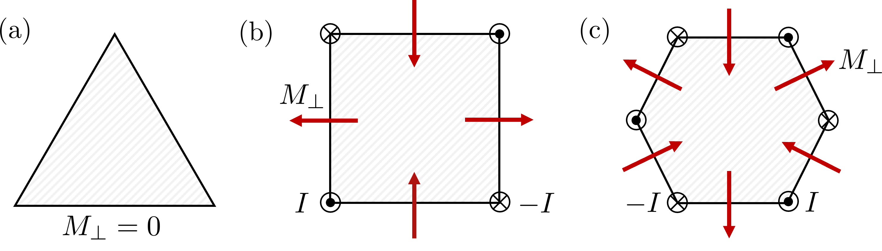
Figure 4: Symmetry constraints arising from $3^{\prime}_{m}$, $4^{\prime}_{m}$, and $6^{\prime}_{m}$ symmetries. Arrows indicate the directions of the surface-normal magnetizations relative to a global Cartesian frame. A hinge current flowing into or out of the page is shown with a cross or dot respectively. (a) Triangular prism construction consistent with $3^{\prime}_{m}$ symmetry. Surfaces have no magnetization. (b) Square prism construction consistent with $4^{\prime}_{m}$ symmetry. Surface magnetizations form a two-in two-out configuration with $M_{\perp}=I/2$. (c) Hexagonal prism construction consistent with $6^{\prime}_{m}$ symmetry. Surface magnetizations form a three-in three-out configuration with $M_{\perp}=I/2$.

In the case of $3^{\prime}_{m}$, symmetry dictates that each facet have vanishing magnetization. For the $4^{\prime}_{m}$ and $6^{\prime}_{m}$ screws, the surface magnetizations may be found from the currents on the prism hinges.

Symmetries of type $S^{+}_{\hat{\textbf{z}}}$.

We construct a surface as in the $S^{-}_{\hat{\textbf{z}}}$ case. Although $S^{+}_{\hat{\textbf{z}}}$ operations leave the surface invariant, they do not flip $M_{\perp}$. We therefore cannot extract any meaningful information from this construction.

However, operations in this class may also relate surfaces with normals not along $\hat{\textbf{z}}$. For the case of $C_{n}$ operations with $n=3,4,6$, we may generate the same infinite prism constructions as in the $N^{-}_{\hat{\textbf{z}}}$ class of operations. However, as we see in Fig. 5, all the hinge currents vanish, and although we know the relative orientations of the facet magnetizations, we cannot extract any information on their magnitudes as a result.

For the $C_{2}$ as well as $m^{\prime}_{d}$ operations, we may construct a slab geometry as in the case of $R^{-}_{\hat{\textbf{z}}}$ operations, except that the $z$-direction will be periodic, and the slab is consistent with either the $C_{2}$ or the $m^{\prime}_{d}$ symmetry. As a result, any possible surface magnetizations will be equal and antiparallel on the two surfaces, as shown for the particular case of an $m^{\prime}_{x}$ symmetry in Fig. 6. With the introduction of an additional arbitrary surface facet, we may attempt to solve a system of equations

$$0 =M^{\text{L}}_{\perp}-M^{\text{R}}_{\perp},$$

$$I_{1} =M^{\text{L}}_{\perp}-M^{\text{F}}_{\perp},$$ (4)

$$I_{2} =M^{\text{F}}_{\perp}-M^{\text{R}}_{\perp},$$

involving the hinge currents. However, this system is unsolvable.

Thus, $S^{+}_{\hat{\textbf{z}}}$ operations alone are unable to unambiguously define surface magnetizations.

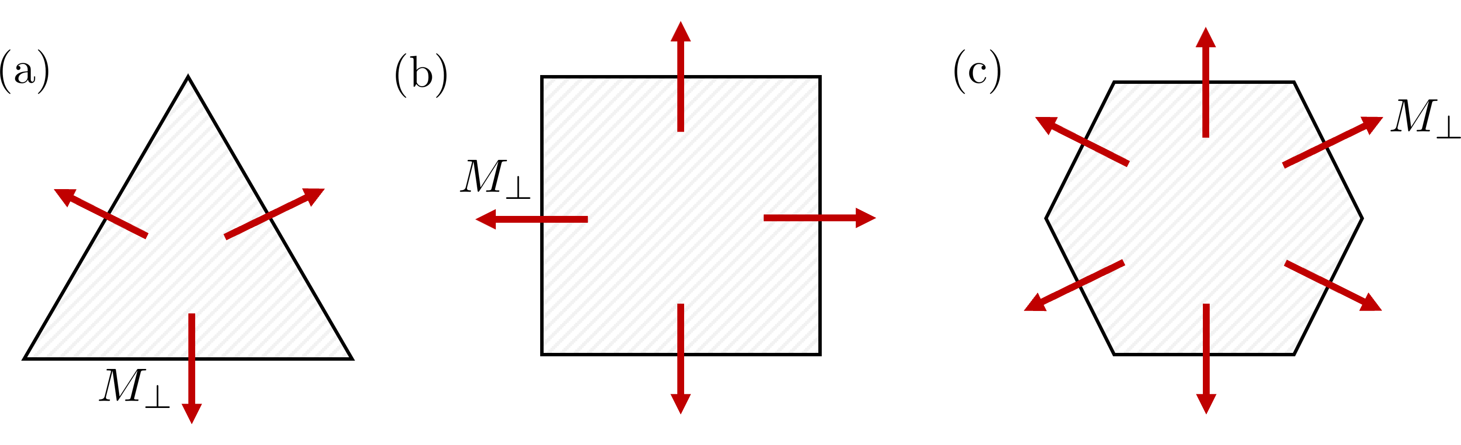
Figure 5: Symmetry constraints arising from $3_{m}$, $4_{m}$, and $6_{m}$ symmetries. Conventions are the same as in Fig. 4. (a) Triangular prism constructed using $3_{m}$ symmetry. (b) Square prism constructed using $4_{m}$ symmetry. (c) Hexagonal prism constructed using $6_{m}$ symmetry. In each case all facets have the same surface magnetization $M_{\perp}$, whose magnitude cannot be determined since hinge currents are absent.

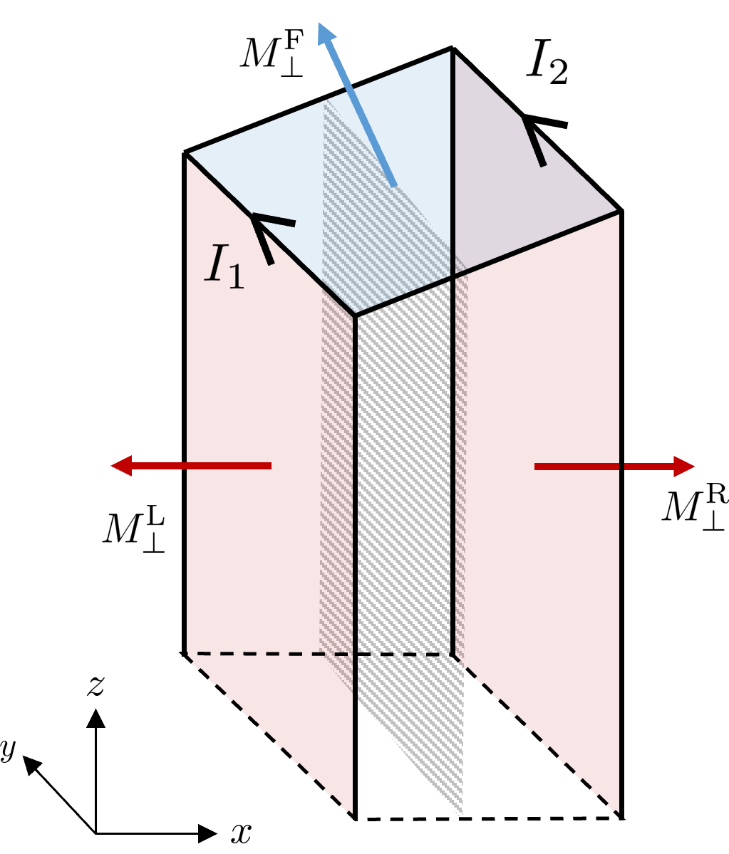
Figure 6: Schematic of a slab geometry respecting an $m^{\prime}_{x}$ symmetry, with the mirror plane illustrated by the thatched gray plane bisecting the slab. An additional facet of arbitrary orientation appears at the top. The $m^{\prime}_{x}$ symmetry ensures that the magnetizations on the left and right facets are equal and antiparallel. In this case the knowledge of the hinge currents is insufficient to determine the $M_{\perp}$ values, as discussed in the text.

Symmetries of type $N^{+}_{\hat{\textbf{z}}}$.

Being nonsymmorphic operations in the $\hat{\textbf{z}}$ direction, no surface with the same unit normal will ever be preserved by an $N^{+}_{\hat{\textbf{z}}}$ operation, so these operations by themselves tell us nothing about magnetizations at this surface. Furthermore, they provide no information on surfaces transverse to the $\hat{\textbf{z}}$ surface, as the arguments in Figs. 5 and 6 apply.

Symmetries of type $R^{+}_{\hat{\textbf{z}}}$.

The same arguments as presented for the $S^{+}_{\hat{\textbf{z}}}$ and $N^{+}_{\hat{\textbf{z}}}$ cases hold here as well. We therefore cannot define surface magnetizations in this case either.

III.3 Discussion

Within a classical context, our symmetry analysis reveals that we may unambiguously define magnetizations on the surfaces only when the bulk symmetry group features $S^{-}_{\hat{\textbf{n}}}$, $R^{-}_{\hat{\textbf{n}}}$, or $N^{-}_{\hat{\textbf{n}}}$ operations.

In these cases, the argument proceeded via a thought experiment involving the construction of a slab or rod in such a way that the surface facets are related to each other by a global application of the relevant bulk symmetry. The facet magnetizations could then be determined from a knowledge of the hinge currents in these geometries. We emphasize that, for these bulk symmetries, the surface magnetizations are still well defined even for configurations in which different facets are terminated in different ways. The conclusion that $M_{\perp}$ is well defined follows just from knowing that it is possible, in principle, to prepare a globally symmetric slab or rod.

As it happens, the $S^{-}_{\hat{\textbf{n}}}$, $R^{-}_{\hat{\textbf{n}}}$, and $N^{-}_{\hat{\textbf{n}}}$ symmetries that allow an unambiguous definition are precisely the ones that are classified as axion-odd according to Table 1. In other words, these are the symmetries that reverse the sign of the Chern-Simons axion (CSA) coupling, which describes a topological contribution to the isotropic linear magnetoelectric coupling of the material Qi et al. (2008); Essin et al. (2009); Varnava et al. (2020). This is characterized by an “axion angle” $\theta_{\text{CS}}$ that takes the form

$$\theta_{\text{CS}}=-\frac{1}{4\pi}\int_{\text{BZ}}\epsilon_{\mu\nu\sigma}\text{Tr}\left[A_{\mu}\partial_{\nu}A_{\sigma}-\frac{2i}{3}A_{\mu}A_{\nu}A_{\sigma}\right]d\textbf{k},$$ (5)

where the integration is performed over the Brillouin zone and $A^{mn}_{\mu}(\textbf{k})=i\langle u_{m\textbf{k}}|\partial_{\mu}u_{n\textbf{k}}\rangle$ is the Berry connection matrix, with $|u_{n\textbf{k}}\rangle$ being the cell-periodic part of the Bloch function of occupied band $n$.

A defining feature of the CSA coupling is that it is gauge-invariant modulo $2\pi$ under a unitary mixing of the occupied ground state Bloch functions. That is, if we perform the transformation

$$|\tilde{u}_{n\textbf{k}}\rangle=\sum^{\text{occ}}_{m}U_{mn}(\textbf{k})|u_{m\textbf{k}}\rangle,$$ (6)

where $U_{mn}(\textbf{k})$ is a unitary matrix, then $\theta_{\text{CS}}\to\theta_{\text{CS}}+2\pi n$ where $n$ is an integer. The operations of the type $S^{-}_{\hat{\textbf{n}}}$, $R^{-}_{\hat{\textbf{n}}}$, and $N^{-}_{\hat{\textbf{n}}}$ reverse the sign of $\theta_{\text{CS}}$; but since the coupling is defined modulo $2\pi$, it follows that $\theta_{\text{CS}}=0\text{ or }\pi$. Thus, the axion angle is quantized to values of 0 or $\pi$ in the presence of axion-odd symmetries. By contrast, an axion-even symmetry (simple rotation or time-reversed improper rotation) allows for a generically nonzero value of $\theta_{\text{CS}}$.

This identification of an intimate connection between the ability to define unambiguous surface magnetizations and the presence of a quantized axion coupling is one of the principle contributions of this work.

While we have been focusing on the consequences of symmetry in this section, this can only take us so far. Even in the axion-odd case where we expect a unique definition of surface magnetization, the symmetry arguments and classical theory do not answer the question of how, in principle, this quantity can be obtained from a direct calculation using only information about the surface Hamiltonian and surface electronic structure of a given surface. In the opposite case that no axion-odd symmetry is present, the same question arises, but now there is the additional issue of a possible shift freedom in the definition of $M_{\perp}$. To go beyond the symmetry arguments, we need to develop an explicit framework for carrying out calculations of surface orbital magnetization in the general case. The remainder of this work is devoted to an exploration of the use of quantum-mechanical orbital-magnetization local markers for the construction of such a framework.

IV Methods

We now turn to a discussion of the computational aspects of surface magnetization and hinge currents. We expand on the local marker formulation of orbital magnetization Bianco and Resta (2013) and discuss its application in computing surface magnetization. The section is concluded with a discussion of microscopic currents and an explanation of their relationship to the macroscopic hinge current.

IV.1 Local-marker formulation

We now work in 3D, where Eq. (1) takes the form

$$\textbf{M}=\frac{1}{V}\int_{V}\mathbfcal{M}(\textbf{r})d\textbf{r}.$$ (7)

Here $V$ is the unit cell volume and both M and $\mathbfcal{M}(\textbf{r})$ have units of magnetic moment per unit volume. (Quantities denoted as $M_{\perp}$ or $M^{\textrm{surf}}$ will continue to be 2D surface magnetizations with units of magnetic moment per unit area.) We focus initially on the single component $M_{z}$ of M, dropping the $z$ subscript for conciseness. The local-marker formulation is a direct result of expressing the orbital magnetization in terms of the single particle density matrix $P(\textbf{r},\textbf{r}^{\prime})$. Bianco and Resta Bianco and Resta (2013) demonstrated that for bulk insulating systems at $T=0$ at the single-particle level, where $P^{2}=P$, the magnetization $M$ may be written as

$$M=M_{\text{LC}}+M_{\text{IC}}+M_{\text{C}}$$ (8)

with

$$M_{\text{LC}} = -\frac{e}{\hbar V}\text{Im}\text{Tr}[PxQHQyP],$$ (9)

$$M_{\text{IC}} = \frac{e}{\hbar V}\text{Im}\text{Tr}[QxPHPyQ],$$ (10)

$$M_{\text{C}} = -\frac{2\mu e}{\hbar V}\text{Im}\text{Tr}[QxPyQ],$$ (11)

where $e<0$ is the electron charge, the trace is taken per unit cell of volume $V$, $Q=1-P$, $H$ is the Hamiltonian, and $\mu$ is the Fermi energy. $M_{\text{LC}}$, $M_{\text{IC}}$, and $M_{\text{C}}$ correspond to the so-called local circulation, itinerant circulation, and Chern number contributions to the magnetization, respectively Ceresoli et al. (2006).

Eq. (7), expressing the total $M$ as a trace of a local marker $\mathcal{M}(\textbf{r})$ over position space, is evidently satisfied by choosing

$$\mathcal{M}(\textbf{r})=\mathcal{M}_{\text{LC}}(\textbf{r})+\mathcal{M}_{\text{IC}}(\textbf{r})+\mathcal{M}_{\text{C}}(\textbf{r}),$$ (12)

with

$$\mathcal{M}_{\text{LC}}(\textbf{r}) = -\frac{e}{\hbar}\text{Im}\langle\textbf{r}|PxQHQyP|\textbf{r}\rangle,$$ (13)

$$\mathcal{M}_{\text{IC}}(\textbf{r}) = \frac{e}{\hbar}\text{Im}\langle\textbf{r}|QxPHPyQ|\textbf{r}\rangle,$$ (14)

$$\mathcal{M}_{\text{C}}(\textbf{r}) = -\frac{2\mu e}{\hbar}\text{Im}\langle\textbf{r}|QxPyQ|\textbf{r}\rangle.$$ (15)

Note that $\mathcal{M}_{\text{C}}(\textbf{r})$ is directly proportional to the local Chern marker $C(\textbf{r})$ Bianco and Resta (2011); Rauch et al. (2018), i.e.,

$$\mathcal{M}_{\text{C}}(\textbf{r})=-\frac{2\mu e}{\hbar}\text{Im}\langle\textbf{r}|QxPyQ|\textbf{r}\rangle=-\frac{e\mu}{h}C(\textbf{r}),$$ (16)

consistent with the discussion towards the end of Sec. III.3.

It is important to note that due to the invariance of the trace under cyclic permutations of operators, different expressions for $\mathcal{M}(\textbf{r})$ stemming from Eq. (8) are possible. For example, $\mathcal{M}_{\text{LC}}(\textbf{r})$ in Eq. (12) could be replaced by

$$\mathcal{M}^{\cal L}_{\text{LC}}(\textbf{r})=-\frac{e}{\hbar}\text{Im}\langle\textbf{r}|HQyPxQ|\textbf{r}\rangle$$ (17)

or

$$\mathcal{M}^{\cal R}_{\text{LC}}(\textbf{r})=-\frac{e}{\hbar}\text{Im}\langle\textbf{r}|QyPxQH|\textbf{r}\rangle,$$ (18)

achieved by applying a cyclic permutation to $\mathcal{M}_{\text{LC}}(\textbf{r})$ in Eq. (13) and using the fact that $Q^{2}=Q$. The $\cal L$ and $\cal R$ superscripts indicate that $H$ has been moved to the “left” or “right” respectively, and henceforth we shall refer to the marker in Eq. (13) as $\mathcal{M}^{\cal C}_{\text{LC}}$ ($\cal C$ for “center”). Integrating Eq. (17) or (18) over all space yields Eq. (9), just as integrating Eq. (13) does. We refer to the different expressions for the local marker as trace projections. Such an ambiguity in the local marker may be viewed as a manifestation of the fact that microscopic magnetic dipole densities are not well defined.

As we will see in the following subsections, there is no such ambiguity with respect to cyclic permutation of operators for the local Chern marker $C({\bf r})$, which is therefore well defined at a specific ${\bf r}$ in the context of a marker-based theory. As a result of Eq. (16), this implies that $\mathcal{M}_{\text{C}}({\bf r})$ has a linear dependence on the chemical potential $\mu$ as it is scanned across the gap. This observation allowed Zhu et al. Zhu et al. (2021) to introduce a uniquely defined “surface magnetic compressibility” $dM_{\perp}/d\mu$ in terms of the presence of a net coarse-grained Chern-marker concentration at the surface. We note in passing that the Chern marker is closely related to the local anomalous Hall conductivity, i.e., the antisymmetric part of the surface conductivity tensor $\sigma_{ij}({\bf r})=\partial j_{i}({\bf r})/\partial E_{j}$ describing the first-order response of the local current density ${\bf j}({\bf r})$ to a homogeneous macroscopic electric field $\bf E$. However, as shown by Rauch et al. Rauch et al. (2018), the two are not identical, since the local anomalous Hall conductivity also contains a non-geometric or “cross-gap” term that is not captured by the Chern marker.

In the following subsections, we discuss several physical requirements that we impose on the markers, allowing us to reduce the number of candidates to just a few that can be regarded as physically acceptable.

IV.1.1 Independence of origin

We first require that the trace projections should be independent of origin. A potential marker $\mathcal{M}^{[P,Q,H]}({\bf r})$ may be regarded as depending on the system-specific operators $P$, $Q$, and $H$ as indicated by the superscript notation. Introducing the unitary operator $T$ for a translation by displacement $\bf t$, and defining translated operators $\tilde{P}=TPT^{\dagger}$ and similarly for $Q$ and $H$, the desired independence of origin is equivalent to asking that $\mathcal{M}^{[P,Q,H]}({\bf r})=\mathcal{M}^{[\tilde{P},\tilde{Q},\tilde{H}]}({\bf r}+{\bf t})$. We accomplish this by insisting that the markers be written in terms of the operators

$$X=PxQ,\quad Y=PyQ,\quad Z=PzQ$$ (19)

and their Hermitian conjugates. A combination like $P{\bf r}Q$ transforms to $\tilde{P}\tilde{{\bf r}}\tilde{Q}=\tilde{P}({\bf r}-{\bf t})\tilde{Q}=\tilde{P}{\bf r}\tilde{Q}$, where the last equality follows from the fact that $PQ=0$. Thus, expressions built out of the operators in Eq. (19) will automatically satisfy the desired independence of origin. With this notation, Eqs. (13), (17), and (18) become

$$\mathcal{M}^{\cal C}_{\text{LC}}({\bf r}) = -\frac{e}{\hbar}\text{Im}\langle{\bf r}|XHY^{\dagger}|{\bf r}\rangle,$$ (20)

$$\mathcal{M}^{\cal L}_{\text{LC}}({\bf r}) = -\frac{e}{\hbar}\text{Im}\langle{\bf r}|HY^{\dagger}X|{\bf r}\rangle,$$ (21)

$$\mathcal{M}^{\cal R}_{\text{LC}}({\bf r}) = -\frac{e}{\hbar}\text{Im}\langle{\bf r}|Y^{\dagger}XH|{\bf r}\rangle.$$ (22)

Other choices such as $\langle{\bf r}|yPxQHQ|{\bf r}\rangle$ would not satisfy this property. At this point, then, we have three candidates for the LC marker, and there is a corresponding set of three choices for the IC marker.

As for the Chern-marker contribution, similar considerations imply that $\mathcal{M}_{\text{C}}(\textbf{r})$ should also be written in terms of $X$ and $Y$ operators. Eq. (15) then leads to $\mathcal{M}_{\text{C}}(\textbf{r})=-(2\mu e/\hbar)\text{Im}\langle\textbf{r}|X^{\dagger}Y|\textbf{r}\rangle=(2\mu e/\hbar)\text{Im}\langle\textbf{r}|Y^{\dagger}X|\textbf{r}\rangle$. Further algebra demonstrates that these expressions are identical with $\mathcal{M}_{\text{C}}(\textbf{r})=(2\mu e/\hbar)\text{Im}\langle\textbf{r}|XY^{\dagger}|\textbf{r}\rangle=-(2\mu e/\hbar)\text{Im}\langle\textbf{r}|YX^{\dagger}|\textbf{r}\rangle$ (see Eq. (A14) of the Appendix of Ref. Rauch et al. (2018)). Thus, we are left with a unique expression for $\mathcal{M}_{\text{C}}(\textbf{r})$, as well as the local Chern marker itself.

IV.1.2 Covariance under rotations

We next insist that the markers should transform as vectors under global rotations of the system. That is, given a spatial rotation $\mathcal{R}$ and its corresponding unitary operator $\mathfrak{R}$, we ask that $\mathcal{M}^{[P,Q,H]}({\bf r})=\mathcal{R}^{-1}\mathcal{M}^{[\tilde{P},\tilde{Q},\tilde{H}]}(\mathcal{R}{\bf r})$, where $\tilde{P}=\mathfrak{R}P\mathfrak{R}^{\dagger}$, etc. In particular, we insist that any candidate for the marker $z$ component should be invariant under rotation by an arbitrary angle $\theta$ about $\hat{\bf z}$. For $\theta=\pi/2$ we have $X\rightarrow Y$ and $Y\rightarrow-X$, and using the general formula $\text{Im}\langle\cal O\rangle=-\text{Im}\langle\cal O^{\dagger}\rangle$, we find that $\mathcal{M}^{\cal C}_{\text{LC}}$ is invariant while $\mathcal{M}^{\cal L}_{\text{LC}}$ and $\mathcal{M}^{\cal R}_{\text{LC}}$ transform into one another. Thus, neither $\mathcal{M}^{\cal L}_{\text{LC}}$ nor $\mathcal{M}^{\cal R}_{\text{LC}}$ satisfies rotational invariance by itself, but at least for $\theta=\pi/2$, the average $(\mathcal{M}^{\cal L}_{\text{LC}}+\mathcal{M}^{\cal R}_{\text{LC}})/2$ does.

A more careful check confirms that this combination is also invariant under arbitrary rotations by angle $\theta$. We can therefore propose two valid local-circulation markers,

$$\mathcal{M}^{\cal C}_{\text{LC},z}({\bf r}) = -\frac{e}{\hbar}\text{Im}\langle{\bf r}|XHY^{\dagger}|{\bf r}\rangle,$$ (23)

$$\mathcal{M}^{\cal E}_{\text{LC},z}({\bf r}) = -\frac{e}{2\hbar}\text{Im}\langle{\bf r}|\{H,Y^{\dagger}X\}|{\bf r}\rangle,$$ (24)

where the $z$ subscript has temporarily been restored, and the $\cal E$ superscript in the second equation involving the anticommutator indicates that $H$ is in an “external” (left or right) position. More generally, we can define vector markers $\mathbfcal{M}_{\text{LC}}$ whose $x$ and $y$ components have the same form as in Eqs. (23) and (24) but with a cyclic permutation of the Cartesian indices. Since any rotation can be written as a product of three consecutive rotations around Cartesian axes by Euler angles, and since our markers have the correct rotation properties under each of these separately, it follows that the overall rotational properties are guaranteed. That is, the rotation of the marker is consistent with the rotation of the system.

The same reasoning applies to the itinerant circulation markers

$$\mathcal{M}^{\cal C}_{\text{IC}}({\bf r}) = \frac{e}{\hbar}\text{Im}\langle{\bf r}|X^{\dagger}HY|{\bf r}\rangle,$$ (25)

$$\mathcal{M}^{\cal E}_{\text{IC}}({\bf r}) = \frac{e}{2\hbar}\text{Im}\langle{\bf r}|\{H,YX^{\dagger}\}|{\bf r}\rangle,$$ (26)

where we have reverted to dropping the $z$ subscript. Combining with Eqs. (23) and (24), we can arrive at several suitable expressions for the full marker in Eq. (12). If we consistently use the center or external versions, we arrive at two choices

$$\mathcal{M}^{\mathcal{C},\mathcal{C}}(\textbf{r}) = \mathcal{M}^{\mathcal{C}}_{\text{LC}}(\textbf{r})+\mathcal{M}^{\mathcal{C}}_{\text{IC}}(\textbf{r}),$$ (27)

$$\mathcal{M}^{\mathcal{E},\mathcal{E}}(\textbf{r}) = \mathcal{M}^{\mathcal{E}}_{\text{LC}}(\textbf{r})+\mathcal{M}^{\mathcal{E}}_{\text{IC}}(\textbf{r}).$$ (28)

We also consider a third marker involving a mixed choice,

$$\mathcal{M}^{\mathcal{C},\mathcal{E}}(\textbf{r}) = \mathcal{M}^{\mathcal{C}}_{\text{LC}}(\textbf{r})+\mathcal{M}^{\mathcal{E}}_{\text{IC}}(\textbf{r}).$$ (29)

We could also introduce its partner $\mathcal{M}^{\mathcal{E},\mathcal{C}}$, but there are actually only three linearly independent markers, since it is easy to show that $\mathcal{M}^{\mathcal{C},\mathcal{E}}+\mathcal{M}^{\mathcal{E},\mathcal{C}}=\mathcal{M}^{\mathcal{C},\mathcal{C}}+\mathcal{M}^{\mathcal{E},\mathcal{E}}$.

For the Chern marker contribution of Eqs. (15-16), it is easy to see that for arbitrary rotations $\theta$ about $\hat{\textbf{z}}$ we have $\mathcal{M}_{\text{C}}(\textbf{r})=-(2\mu e/\hbar)\text{Im}\langle\textbf{r}|X^{\dagger}Y|\textbf{r}\rangle\to(2\mu e/\hbar)\text{Im}\langle\textbf{r}|Y^{\dagger}X|\textbf{r}\rangle=\mathcal{M}_{\text{C}}(\textbf{r})$. We may then define a vector marker $\mathbfcal{M}_{\text{C}}$ analogously to $\mathbfcal{M}_{\text{LC}}$, and the former is found to exhibit rotational covariance for the same reasons as the latter.

IV.1.3 Transformation under $H\rightarrow-H$

Our third requirement is based on the following observation regarding the behavior of microscopic currents. As will be shown later in this section, the microscopic current density at r is given by

$$\textbf{j}(\textbf{r})=\frac{e}{\hbar}\int d\textbf{r}^{\prime}(\textbf{r}-\textbf{r}^{\prime})\text{Im}[\langle\textbf{r}^{\prime}|P|\textbf{r}\rangle\langle\textbf{r}|H|\textbf{r}^{\prime}\rangle].$$ (30)

Under a transformation that acts to change the overall sign of $H$, the occupied and unoccupied state manifolds are switched; that is, $P^{\prime}=Q$ and $Q^{\prime}=P$. Substituting $H^{\prime}=-H$ and $P^{\prime}$ into Eq. (30), and using the facts that $Q=1-P$ and that the expectation value of a Hermitian operator is real, it is easy to see that $\textbf{j}(\textbf{r})$ is left unchanged. Therefore, the surface magnetizations and hinge currents must be left unchanged as well.

When $H\to-H$, we see that $X\to X^{\dagger}$, $Y\to Y^{\dagger}$, and $Z\to Z^{\dagger}$. It is then readily apparent that $\mathcal{M}^{\mathcal{C},\mathcal{C}}\to\mathcal{M}^{\mathcal{C},\mathcal{C}}$ and $\mathcal{M}^{\mathcal{E},\mathcal{E}}\to\mathcal{M}^{\mathcal{E},\mathcal{E}}$. However, surface magnetization from the $\mathcal{M}^{\mathcal{C},\mathcal{E}}$ marker is not left invariant, as $\mathcal{M}^{\mathcal{C},\mathcal{E}}\to\mathcal{M}^{\mathcal{E},\mathcal{C}}$. We therefore eliminate $\mathcal{M}^{\mathcal{C},\mathcal{E}}$ from the list of valid markers.

We note that for the Chern marker contribution of Eqs. (15-16), under such a transformation $C(\textbf{r})\to-C(\textbf{r})$, while $\mu\to-\mu$. Therefore $\mathcal{M}_{\text{C}}(\textbf{r})$ is left invariant.

IV.1.4 Magnetic quadrupole of finite systems

To conclude our list of acceptable marker properties, we turn to a discussion of the possible role of the bulk magnetic quadrupole moment (MQM) in a theory of surface magnetization. Our motivation for considering the MQM stems from the recently developed theory of boundary electric polarization Benalcazar et al. (2017b); Ren et al. (2021); for a crystallite with vanishing bulk polarization, the theory identifies the bulk electric quadrupole moment as contributing to the electric polarization at the surface. By analogy, it would then be unsurprising if the MQM similarly contributed to the magnetization at a surface for systems with zero bulk magnetization. Earlier works have focused on deriving expressions for the MQM within periodic boundary conditions Shitade et al. (2018); Gao and Xiao (2018); Gao et al. (2018), but have not discussed whether or how it manifests itself on the boundary of a bulk.

As a theory of the bulk MQM density for an extended system is not well established, we focus here on the case of an ideal molecular crystal, i.e., a collection of identical independent units, which we refer to as “molecules”, arranged without overlap on a crystal lattice.

Classically, the MQM tensor $Q_{ij}$ of a single molecule is defined in terms of its microscopic current distribution $\textbf{j}(\textbf{r})$ as

$$Q_{ij}=\frac{1}{3}\int(\textbf{r}\times\textbf{j})_{i}\,r_{j}\,d\textbf{r}.$$ (31)

This is a traceless tensor, since

$$Q_{ii}=\frac{1}{3}\int(\textbf{r}\times\textbf{j})\cdot\textbf{r}\,d\textbf{r}=0.$$ (32)

Its antisymmetric part is known as the toroidal moment, while its symmetric part

$$\widetilde{Q}_{ij}=\frac{1}{2}(Q_{ij}+Q_{ji}),$$ (33)

is solely responsible for the quadrupole contribution to the far $\mathbf{B}$ field in the multipole expansion.

When this molecular unit is periodically repeated to generate a large but finite crystallite, the quadrupole moment densities are defined as $\bm{\mathcal{Q}}=\mathbf{Q}/V$ and $\widetilde{\bm{\mathcal{Q}}}=\widetilde{\mathbf{Q}}/V$, where $V$ is the unit cell volume. One can then show that the MQM generates a magnetization at a surface with outward normal $\hat{\textbf{n}}$ given by Raab and De Lange (2004)

$$M^{\textrm{surf}}_{i}=\mathcal{Q}_{ij}n_{j}.$$ (34)

Repackaging the toroidal part of the MQM density as the vector $\mathfrak{m}_{i}=\epsilon_{ijk}\mathcal{Q}_{jk}/2$, it is clear that this produces a surface magnetization $\mathbf{M}^{\textrm{surf}}_{\parallel}=\hat{\textbf{n}}\times\mathfrak{m}$ that is parallel to the surface. This part does not contribute to the surface-normal component $M_{\perp}$, which is just given by

$$M_{\perp}^{(\hat{\mathbf{n}})}=\mathcal{Q}_{ij}n_{i}n_{j}=\hat{\mathbf{n}}^{\mathrm{T}}\cdot\bm{\mathcal{Q}}\cdot\hat{\mathbf{n}}.$$ (35)

We are thus free to insert either the unsymmetrized $\bm{\mathcal{Q}}$ or the symmetrized $\widetilde{\bm{\mathcal{Q}}}$ tensor into Eq. (35) when computing $M_{\perp}$ values, ignoring the toroidal component Dubovik et al. (1986); Dubovik and Tugushev (1990).

We will refer to the MQM tensors defined as in Eq. (31) as current-based quadrupoles. In the special case that the current distribution takes the form of a collection of point magnetic dipoles $\mathbf{m}_{\mu}$ located at sites $\mathbf{r}_{\mu}$, one can introduce an alternative dipole-based definition

$$Q^{\text{dip}}_{ij}=\sum_{\mu}m_{\mu,i}\,r_{\mu,j}.$$ (36)

If one considers the limit that the point dipoles are constructed from small current loops of vanishing size, it turns out that the traceless part of $Q^{\text{dip}}$ is identical with $Q$ (see Appendix C). That is,

$$Q_{ij}=Q^{\text{dip}}_{ij}-\frac{1}{3}\delta_{ij}Q_{kk}^{\text{dip}}.$$ (37)

For a molecular crystal, the dipole formula provides a natural connection to the use of the local magnetization marker. That is, we can calculate the MQM density of the crystal as

$$\mathcal{Q}_{ij}^{\text{dip}}=\frac{1}{V}\int{\cal M}_{i}(\mathbf{r})\,r_{j}\,d^{3}r$$ (38)

or

$$\mathcal{Q}_{ij}^{\text{dip}}=\frac{1}{V}\sum_{\mu}{\cal M}_{\mu,i}\,r_{\mu,j},$$ (39)

where ${\cal M}_{i}(\mathbf{r})$ and ${\cal M}_{\mu,i}$ are the continuum and discrete markers, respectively. Therefore, in the rest of this paper, we will focus on the dipole-based expression in Eq. (39) in the context of our tight-binding calculation of the local markers. We will then remove the trace part in order to compare with the current-based tensor computed from Eq. (31) in the same TB framework.

Tests of this kind will be presented in Sec. V.4. Unlike the other criteria described above in Secs. IV.1.1 to IV.1.3, we do not know how to determine a priori whether a certain marker will satisfy the present criterion of reproducing the MQM correctly for molecular crystals. However, we will see in Sec. V.4 that some choices of marker sometimes fail this test. Thus, even if numerical in nature, these tests provide important constraints on the appropriate choice of marker for the computation of surface magnetization.

We note in passing that the use of the raw dipole-based MQM, without removing the trace part, will generate different results for the surface magnetizations $M_{\perp}$. However, it will shift $M_{\perp}$ equally on all facets, and therefore will still yield a correct prediction of the hinge currents, as these only depend on differences of $M_{\perp}$ on neighboring facets (see Eq. (2)). In this sense, the use of the raw dipole-based MQM in place of the traceless one is reminiscent of the shift freedom in the definition of $M_{\perp}$ discussed in the Introduction, here for the case of an idealized molecular crystal.

IV.1.5 Discussion

The considerations of Secs. IV.1.1-IV.1.3 have reduced the list of acceptable markers to the two given in Eqs. (27-28), augmented by the uniquely defined Chern-marker contribution $\mathcal{M}_{\text{C}}({\bf r})$. The marker $\mathcal{M}^{\mathcal{C},\mathcal{C}}$ of Eq. (27) is the original one of Bianco and Resta Bianco and Resta (2013), while $\mathcal{M}^{\mathcal{E},\mathcal{E}}$ of Eq. (28) is a new candidate that has not, to our knowledge, been considered previously. We also note that there is no restriction on using a linear combination of $\mathcal{M}^{\mathcal{C},\mathcal{C}}$ and $\mathcal{M}^{\mathcal{E},\mathcal{E}}$ to write down a new marker, as long the linear combination reproduces the bulk magnetization $M$ of Eq. (8). To maintain this requirement, the (real) coefficients $a_{\mathcal{CC}}$ and $a_{\mathcal{EE}}$ of the linear combination must sum to unity.

We select the particular linear combination $(a_{\mathcal{CC}},a_{\mathcal{EE}})=(1/3,2/3)$ to form the “linear” marker

$$\mathcal{M}^{\text{lin}}(\textbf{r})=\frac{1}{3}\mathcal{M}^{\mathcal{C},\mathcal{C}}(\textbf{r})+\frac{2}{3}\mathcal{M}^{\mathcal{E},\mathcal{E}}(\textbf{r}).$$ (40)

This marker is also expressible as

$$\mathcal{M}^{\text{lin}}(\textbf{r})=\frac{1}{3}\mathcal{M}^{\mathcal{C},\mathcal{C}}(\textbf{r})+\frac{1}{3}\mathcal{M}^{\mathcal{L},\mathcal{L}}(\textbf{r})+\frac{1}{3}\mathcal{M}^{\mathcal{R},\mathcal{R}}(\textbf{r}),$$ (41)

i.e. it is the arithmetic average of the $\mathcal{M}^{\mathcal{C},\mathcal{C}}$, $\mathcal{M}^{\mathcal{L},\mathcal{L}}$, and $\mathcal{M}^{\mathcal{R},\mathcal{R}}$ markers. Such a choice might heuristically be justified by noting that since we have no reason to prefer any one of Eqs. (20-22), we choose an equally weighted average of all three of them. For the rest of this paper, we will focus on the markers $\mathcal{M}^{\mathcal{C},\mathcal{C}}$ and $\mathcal{M}^{\mathcal{E},\mathcal{E}}$ of Eqs. (27-28) and $\mathcal{M}^{\text{lin}}$ of Eq. (40) when reporting the results of numerical tests.

Having formulated our list of markers, we are faced with several questions regarding their behavior. First, it remains to be seen which, if any, of the markers will correctly predict the hinge current. For each of the two surfaces forming a hinge, identical markers will be used to compute their respective magnetizations, which in turn will be substituted into Eq. (2) to yield the hinge current. In such tests, it is of interest to check whether there is a dependence on the presence of axion-odd vs. axion-even symmetries. Recall that at the level of classical electromagnetism, only differences of the magnetizations of surface facets sharing a hinge are generally well defined. As an exception, when axion-odd symmetries are present, the $M_{\perp}$ values can be determined from a knowledge of the hinge currents. We should then like to see whether the quantum marker-based theory is also better behaved when axion-odd symmetries are present, and whether, in the absence of such symmetries, the shift freedom of the classical framework reappears at the quantum level. This would be signaled by the existence of multiple markers correctly predicting the hinge currents but differing by a constant shift for all facets.

Before attempting to answer these questions, we discuss some technicalities of the computation of the surface magnetization from the local markers.

IV.2 Surface magnetization and macroscopic averaging

Recall that we assume that the system has enough symmetry to force the macroscopic magnetization to vanish in the bulk. However, this does not necessarily imply that $\mathcal{M}(\textbf{r})$ vanishes everywhere, only that its bulk unit cell average vanishes. In case $\mathcal{M}(\textbf{r})$ does vanish identically deep in the bulk, then for any given trace projection, it is straightforward to integrate $\mathcal{M}(\textbf{r})$ over one surface unit cell, with the surface-normal integral carried deep enough into bulk and vacuum, to obtain a corresponding macroscopic surface magnetization. If this is not the case, however, a coarse-graining procedure is required, as described next.

We construct an insulating slab of thickness $L$ with the outward normals at the top and bottom surfaces being $\hat{\textbf{z}}$ and $-\hat{\textbf{z}}$ respectively, and with cell-periodic boundary conditions in $x$ and $y$. The slab features the maximal symmetry allowed by the bulk. We assume $L>>c$, where $c$ is the lattice constant in the surface-normal direction. We define a “layer-resolved” local marker by averaging the local marker over an in-plane unit cell of area $A$ at fixed $z$:

$$\overline{\mathcal{M}}(z)=\frac{1}{A}\int_{A}\mathcal{M}(x,y,z)\,dx\,dy.$$ (42)

Note that the total magnetization of the slab (magnetic moment per unit area) is the integral of $\overline{\mathcal{M}}(z)$ over the thickness of the slab.

The macroscopic surface magnetization is determined from the application of a smoothening procedure for the layer-resolved marker, since simple sums of the marker may not be convergent. We employ the sliding window average approach to compute the surface magnetization; for details on this method, we refer the reader to Sec. IV.A of Ref. Ren et al. (2021). In numerical work, the averaging amounts to an integration of the local marker weighted by a “ramp function” that extends sufficiently deep in the bulk. The ramp-down function is defined as

$$f_{d}(u)=\begin{cases}1,\text{ if }u<0\\ 1-u/d,\text{if }u\in[0,d]\\ 0,\text{ if }u>d\end{cases}.$$ (43)

Letting the bottom surface of the slab be located at $z=0$, we then get

$$M_{\perp}=\int\overline{\mathcal{M}}(z)f_{c}(z-z_{0})\,dz,$$ (44)

where the range of $z$ integration runs from deep in the vacuum to deep in the interior of the crystal. The result is independent of $z_{0}$ so long as it is sufficiently deep in the bulk region of the slab.

The formalism for the calculation of a surface magnetization has been presented here in the context of a continuum-space treatment. However, our numerical tests will be performed on discrete TB models; in this setting, Eqs. (42) and (44) are expressed as discrete sums over TB sites, where the local markers are now defined. For further details, we refer the reader to Appendix A.

IV.3 Macroscopic hinge current and macroscopic averaging

A direct calculation of the macroscopic hinge current $I$ is necessary in order to test whether it is correctly predicted by each of the various trace projections. The calculations will be accomplished via a macroscopic averaging procedure analogous to that of Sec. IV.2, but now applied to the integration of the microscopic current density over the appropriate hinge region. In this section and in the rest of the paper, we label vector operators with a hat in order to distinguish them from ordinary vectors.

The microscopic current density $\textbf{j}(\textbf{r})$ is obtained from the expectation value of the microscopic current density operator $\hat{\textbf{j}}(\textbf{r})$. Given a single-particle Hamiltonian $H$, this is given by

$$\hat{\textbf{j}}(\textbf{r})=\frac{e}{2}(|\textbf{r}\rangle\langle\textbf{r}|\hat{\textbf{v}}+\hat{\textbf{v}}|\textbf{r}\rangle\langle\textbf{r}|)$$ (45)

where $\hat{\textbf{v}}=(1/i\hbar)[\hat{\textbf{r}},H]$ is the velocity operator. $\textbf{j}(\textbf{r})$ is then obtained as $\text{Tr}[P\hat{\textbf{j}}(\textbf{r})]$, i.e., the trace of $\hat{\textbf{j}}(\textbf{r})$ against the singe-particle density matrix $P$, so that

$$\textbf{j}(\textbf{r})=\frac{e}{\hbar}\int d\textbf{r}^{\prime}(\textbf{r}-\textbf{r}^{\prime})\text{Im}[\langle\textbf{r}^{\prime}|P|\textbf{r}\rangle\langle\textbf{r}|H|\textbf{r}^{\prime}\rangle].$$ (46)

Our calculations of the macroscopic current are performed on a series of insulating infinite rod geometries that retain periodic boundary conditions along one of the three Cartesian directions, as illustrated in Fig. 7. For concreteness, in this subsection we focus on computing the hinge current $I^{\text{FB}}$ for a rod running parallel to the $x$-axis, with unit-cell periodicity $a$. Let the rod have width $W$ along $y$ and height $L$ along $z$, with $W$ and $L$ much larger than the cell dimensions $b$ and $c$ along these respective dimensions.

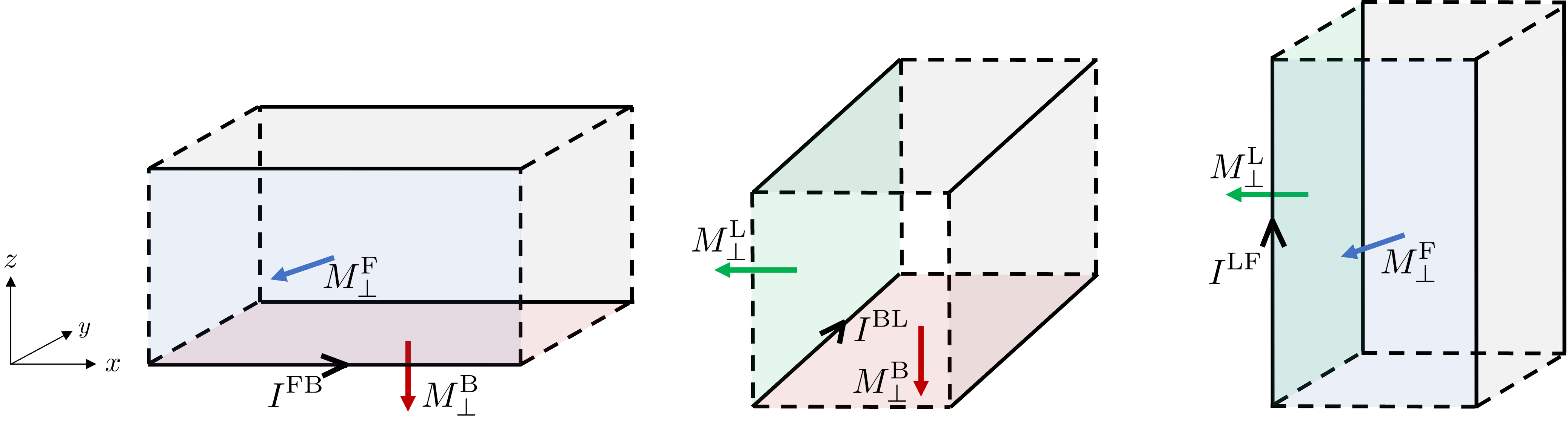
Figure 7: Insulating rod geometries utilized in computing macroscopic hinge currents. Each rod is cut out from the bulk, and satisfies periodic boundary conditions along one of the three Cartesian directions. The surface magnetizations $M^{\text{L}}_{\perp}$, $M^{\text{B}}_{\perp}$, and $M^{\text{L}}_{\perp}$ are determined from calculations described in Sec. IV.2. The macroscopic hinge currents $I^{\text{FB}}$, $I^{\text{BL}}$, and $I^{\text{LF}}$ that are computed in the text are indicated by the black arrows.

In analogy with the surface magnetization, the macroscopic current is obtained from a sliding window average performed over the microscopic currents at the corresponding hinge, but now in two dimensions. The appropriate weight function $w(y,z)$ is a product of two ramp functions in $y$ and $z$, namely $w(y,z)=f_{b}(y-y_{0})f_{c}(z-z_{0})$ where $y_{0}$ and $z_{0}$ are located sufficiently deep within the interior of the rod. $I^{\text{FB}}$ is then given by

$$I^{\text{FB}}=\frac{1}{a}\int^{a}_{0}dx\iint dy\,dz\,j_{x}(x,y,z)w(y,z),$$ (47)

where the range of integration is over all $y$ and $z$.

The currents $I^{\text{BL}}$ and $I^{\text{LF}}$ are computed analogously with the appropriate cell parameters and Cartesian variables used in Eq. (47). As in the previous subsection, the formalism here is developed in the context of a continuum. In a TB formulation, Eqs. (46) and (47) will turn into discrete sums over TB sites. We refer the reader to Appendix B for further details.

V Numerical Results

To test the results of the symmetry analysis of Sec. III and the local marker calculation of surface magnetization, we study three tight-binding (TB) models of spinless electrons. The first model is comprised of an infinite stack of the Haldane-model layers, while the other two models are composed of stacks of two-dimensional (2D) square-plaquette layers. Each model features symmetry-enforced zero bulk magnetization and is considered at half-filling. The TB basis orbitals are assumed to have no orbital moment of their own and to diagonalize the position operators.

We focus on the variation of a single parameter in the Hamiltonian away from the special value that quantizes the CSA coupling, and investigate how the surface magnetization found from the various trace projections behaves as a function of this variation. For each model, the Fermi energy is set to zero, allowing us to neglect the Chern marker contribution to the local magnetization marker.

We use the slab and rod geometries outlined in Secs. IV.2 and IV.3 to compute the surface magnetizations and hinge currents, respectively. Fig. 7 illustrates the particular magnetizations and hinge currents that we compute. The surface magnetizations are found from the coarse-graining procedure described in Sec. IV.2 while the macroscopic hinge currents are found from the coarse-graining procedure of Sec IV.3. Slab and rod geometries for the computation of surface magnetizations and hinge currents are generated by truncating the bulk, i.e., the hoppings to vacant sites are removed while other hoppings and site energies are unchanged. The electronic Hamiltonians for bulk, slab, and rod geometries are constructed and solved using the PythTB code package pyt .

Details of our numerical results will be given in Appendix D. For each model, however, we provide here two tables to demonstrate the behavior of the surface magnetization and hinge currents for the axion-odd regime, as well as a representative axion-even setup. Each table reports the values of $M^{\text{B}}_{\perp}$, $M^{\text{F}}_{\perp}$, and $M^{\text{L}}_{\perp}$ computed from the different markers. The tables also display the differences $\Delta M^{\text{FB}}$, $\Delta M^{\text{BL}}$, and $\Delta M^{\text{LF}}$ between 2D surface magnetizations at different surface facets found from Eq. (44) using identical markers. For example, $\Delta M^{\text{FB}}$ indicates the difference $M^{\text{F}}_{\perp}-M^{\text{B}}_{\perp}$. These are then compared to the appropriate directly computed hinge currents displayed in the bottom-most rows of the tables.

At the end of this section, we numerically address the question of which local marker is able to reproduce the current-based MQM for a finite system with no magnetic moment. We perform a test on a finite cubic model, and compare the current-based MQM tensor to the dipole-based MQM tensors derived from the $\mathcal{M}^{\mathcal{C},\mathcal{C}}$, $\mathcal{M}^{\mathcal{E},\mathcal{E}}$, and $\mathcal{M}^{\text{lin}}$ local markers.

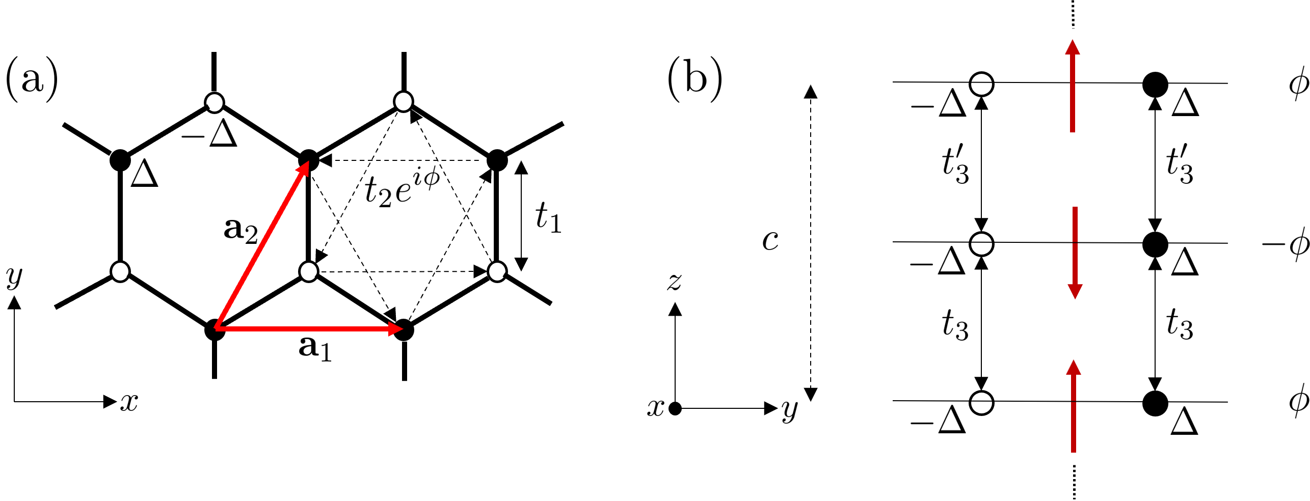
Figure 8: (a) Visualization of a single Haldane layer. The different sublattices are indicated by filled and empty circles, respectively, and feature onsite potentials $\Delta$ and $-\Delta$. The nearest neighbor hopping $t_{1}$ is indicated by the double-sided solid arrow, while the complex next nearest neighbor hopping $t_{2}e^{i\phi}$ is indicated by one-sided dashed arrows. (b) A side view of the bulk unit cell along the $-x$ direction for the model of Sec V.1. The vertical interlayer hoppings connect identical sublattices and are indicated by solid double-sided arrows that are labeled with the corresponding hopping amplitude. Crimson arrows indicate the magnetizations of the layers in the decoupled regime. To the right are the phases of the complex intralayer hoppings.

Table 3: Surface magnetizations and hinge currents (in units of $10^{-5}e/\hbar$) for the alternating Haldane model with $t^{\prime}_{3}=0.1$ (axion-odd).

	$M_{\perp}^{\text{B}}$	$M_{\perp}^{\text{F}}$	$M_{\perp}^{\text{L}}$	$\Delta M^{\text{FB}}$	$\Delta M^{\text{BL}}$	$\Delta M^{\text{LF}}$
$M^{\cal CC}$	1.8082	0.0000	0.0000	$-$1.8082	1.8082	0.0000
$M^{\cal EE}$	1.8082	0.0000	0.0000	$-$1.8082	1.8082	0.0000
$M^{\text{lin}}$	1.8082	0.0000	0.0000	$-$1.8082	1.8082	0.0000
$I_{\text{calc}}$				$-$1.8082	1.8082	0.0000

V.1 Alternating Haldane model

The first model we study consist of half-filled Haldane-model layers Haldane (1988) placed directly on top of each other, which are then subsequently coupled via interlayer hoppings along the $(001)$ direction. The interlayer hoppings couple sites on identical sublattices, and alternate in value from one interlayer region to the next. The intralayer parameters are chosen to be such that if the layers were decoupled, their Chern numbers would vanish and their orbital magnetizations would form an up-down pattern akin to the magnetic moments of an A-type antiferromagnet. The layers are equidistantly spaced, with two layers per unit cell. Figs. 8(a)-(b) provide detailed illustrations of the lattice structure as well as the hoppings and onsite energies of the model. In our calculations we set the lattice vectors as $\textbf{a}_{1}=\hat{\textbf{x}}$, $\textbf{a}_{2}=\frac{1}{2}\hat{\textbf{x}}+\frac{\sqrt{3}}{2}\hat{\textbf{y}}$, and $\textbf{a}_{3}=\hat{\textbf{z}}$.

The symmetries of this model ensure that the bulk magnetization is zero. In particular, there is a three-fold rotation axis $C_{3z}$ about the lattice sites (or honeycomb centers) as well as a time-reversed mirror plane $m^{\prime}_{z}$ passing between the Haldane layers that eliminate the magnetization. Additionally, a time-reversed mirror plane $m^{\prime}_{x}$ bisects the honeycombs along their main diagonals, and a two-fold rotation axis $C_{2y}$ lies between the layers and in the plane of the $m^{\prime}_{x}$ mirror.

The quantization of the CSA coupling is controlled by varying $t^{\prime}_{3}$ while keeping all other parameters fixed. When $t^{\prime}_{3}=t_{3}$, the system gains a time-reversed half-translation $\{E^{\prime}|c/2\}$ symmetry as well as an $m_{z}$ mirror plane residing in the layers; both symmetries are axion-odd.

We adopt the parameter values $\Delta=-1.5$, $t_{1}=-0.1$, $t_{2}=0.15$, $\phi=\pi/4$, $t_{3}=0.1$, and $0.05\leq t^{\prime}_{3}\leq 0.15$. $M^{\text{B}}_{\perp}$ and $M^{\text{F}}_{\perp}$ are found from slabs with six unit cells along $\textbf{a}_{3}$ and eighteen unit cells along $\textbf{a}_{2}$, respectively. The calculation of $M^{\text{L}}_{\perp}$ involves the construction of a supercell with lattice vectors $\textbf{A}_{1}=\textbf{a}_{1}$, $\textbf{A}_{2}=-\textbf{a}_{1}+2\textbf{a}_{2}$, and $\textbf{A}_{3}=\textbf{a}_{3}$. A slab with fifteen cells along $\textbf{A}_{1}$ is then constructed. For $M^{\text{B}}_{\perp}$, $M^{\text{F}}_{\perp}$, and $M^{\text{L}}_{\perp}$, $20\times 20$, $15\times 15$, and $5\times 5$ k-space meshes in reduced coordinates are used, respectively.

Table 4: Surface magnetizations and hinge currents (in units of $10^{-5}e/\hbar$) for the alternating Haldane model with $t^{\prime}_{3}=0.15$ (axion-even).

	$M_{\perp}^{\text{B}}$	$M_{\perp}^{\text{F}}$	$M_{\perp}^{\text{L}}$	$\Delta M^{\text{FB}}$	$\Delta M^{\text{BL}}$	$\Delta M^{\text{LF}}$
$M^{\cal CC}$	1.7970	0.0830	0.0163	$-$1.7140	1.7807	$-$0.0667
$M^{\cal EE}$	1.7970	0.0830	0.0163	$-$1.7140	1.7807	$-$0.0667
$M^{\text{lin}}$	1.7970	0.0830	0.0163	$-$1.7140	1.7807	$-$0.0667
$I_{\text{calc}}$				$-$1.7140	1.7807	$-$0.0667

The macroscopic hinge current $I^{\text{FB}}$ is found from an $x$-extensive rod composed of twenty cells along $\textbf{a}_{3}$ and twenty cells along $\textbf{a}_{2}$. The $y$-extensive rod employed for $I^{\text{BL}}$ is composed of twenty cells along both $\textbf{A}_{1}$ and $\textbf{A}_{3}$, while the $z$-extensive rod for $I^{\text{LF}}$ is composed of twenty cells each along $\textbf{A}_{1}$ and $\textbf{A}_{2}$. For each rod, a 1D k-space sampling of thirty points is employed.

For $t^{\prime}_{3}=0.1$ and $t^{\prime}_{3}=0.15$, respectively, Tables 3 and 4 report the values of the surface magnetizations computed from the different markers. From the tables, we note that for a given surface all three markers yield identical magnetizations, independent of whether or not the system features an axion-odd symmetry. Furthermore, the magnetizations always yield the correct values of the hinge currents. In the axion-odd case of $t^{\prime}_{3}=0.1$, we observe that $M^{\text{F}}_{\perp}$ and $M^{\text{L}}_{\perp}$ may be understood to be zero due to the slab constructions for their calculations featuring the $m_{z}$ mirror plane. By the same token, $I^{\text{LF}}$ vanishes as well, as the $z$ extensive rod used for its calculation also features the same mirror symmetry.

V.2 Two-layer square-plaquette model

Table 5: Surface magnetizations and hinge currents (in units of $10^{-6}e/\hbar$) for the two-layer plaquette model with straight-edge terminations and with $t^{\prime}_{3}=0.1$ (axion-odd).

	$M_{\perp}^{\text{B}}$	$M_{\perp}^{\text{F}}$	$M_{\perp}^{\text{L}}$	$\Delta M^{\text{FB}}$	$\Delta M^{\text{BL}}$	$\Delta M^{\text{LF}}$
$M^{\cal CC}$	2.3768	0.0000	0.0000	$-$2.3768	2.3768	0.0000
$M^{\cal EE}$	2.3768	0.0000	0.0000	$-$2.3768	2.3768	0.0000
$M^{\text{lin}}$	2.3768	0.0000	0.0000	$-$2.3768	2.3768	0.0000
$I_{\text{calc}}$				$-$2.3768	2.3768	0.0000

The model studied here draws inspiration from a 2D square-plaquette model developed in Ref. Ceresoli et al. (2006). As presented there, the model consists of a nearest-neighbor TB Hamiltonian whose primitive cell consists of four sites labeled A-D as shown in Fig. 9(a), with lattice vectors $\textbf{a}_{1}=\hat{\textbf{x}}$ and $\textbf{a}_{2}=\hat{\textbf{y}}$. Each of the four resulting plaquettes in the unit cell is threaded by a magnetic flux that corresponds to endowing some of the hopping amplitudes with an identical complex phase $e^{i\phi/2}$. The moduli of all the nonzero hoppings are set to an identical value $t$.

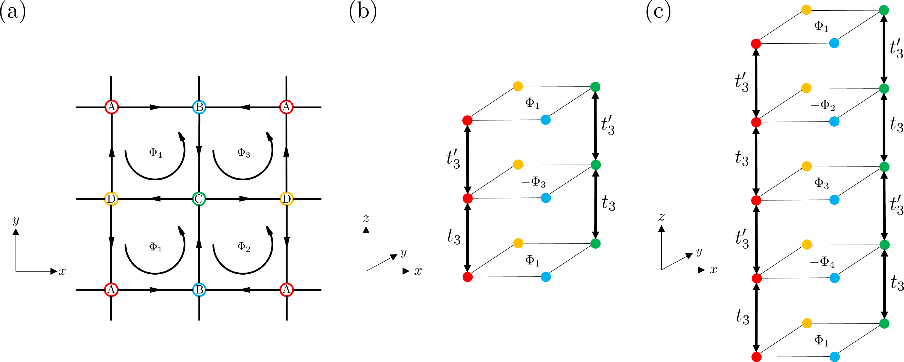
Figure 9: (a) Primitive cell of the 2D square plaquette model. The hoppings between different lattice sites, marked by solid straight lines with arrows, are such that the total flux through the cell is an integer multiple of $2\pi$. (b) Two-layer plaquette model. Only A-A and C-C interlayer hoppings are included, and each layer is related to the one below by a $C^{\prime}_{2z}$ rotation through the $C$ sites. (c) Four-layer plaquette model. Same as (b), except that the rotation is now $C^{\prime}_{4z}$ instead.

Fig. 9(b) provides a detailed illustration of the model that we study. Our model features equidistantly spaced layers of the plaquette model stacked directly on top of one another along the $\hat{\textbf{z}}$ direction. Subsequent layers are related by a time-reversed rotation $C^{\prime}_{2z}$ about a $z$ axis passing through the C site, resulting in two layers per unit cell with $\textbf{a}_{3}=\hat{\textbf{z}}$ forming the third lattice vector. The onsite energies are chosen to be $(E_{A},E_{B},E_{C},E_{D})=(\Delta,-\Delta,\Delta,-\Delta)$ for all layers, consistent with the rotational symmetry. Only interlayer A-A and C-C hoppings are included, with these alternating between $t_{3}$ and $t^{\prime}_{3}$ for subsequent layers. Finally, the chosen flux pattern for the bottom layer is $(\Phi_{1},\Phi_{2},\Phi_{3},\Phi_{4})=(2\phi,-\phi,0,-\phi)$ and the rest of the nearest neighbors are coupled by real and nonzero hoppings $t$ (the modulus of the complex hoppings). The parameter values are chosen such that the layers have a vanishing Chern number in the decoupled limit.

This model possesses a time-reversed inversion symmetry $I^{\prime}$ about a point located midway between C sites on neighboring layers, as well as a two-fold rotation $C_{2x\overline{y}}$ about an axis located between layers and passing above A and C sites. Additionally, there are $m^{\prime}_{xy}$ and $m^{\prime}_{x\overline{y}}$ mirror planes that pass through sites B and D, and A and C, respectively. There is also a time reversed glide mirror plane $\{m^{\prime}_{z}|\bm{\tau}/2\}$ passing in between layers with $\bm{\tau}=\hat{\textbf{x}}+\hat{\textbf{y}}$. These symmetries ensure that the bulk magnetization remains zero.

The CSA coupling is tuned by keeping all parameters fixed except $t^{\prime}_{3}$. If $t_{3}$ and $t^{\prime}_{3}$ are equal, the model gains an axion-odd $\{C^{\prime}_{2z}|c/2\}$ screw axis passing through the C sites. The parameters for this model are chosen as $\Delta=-0.5$, $t=0.06$, $\phi=\pi/4$, $t_{3}=0.1$, and $0.05\leq t^{\prime}_{3}\leq 0.15$.

Table 6: Surface magnetizations and hinge currents (in units of $10^{-6}e/\hbar$) for the two-layer plaquette model with straight-edge terminations and with $t^{\prime}_{3}=0.15$ (axion-even).

	$M_{\perp}^{\text{B}}$	$M_{\perp}^{\text{F}}$	$M_{\perp}^{\text{L}}$	$\Delta M^{\text{FB}}$	$\Delta M^{\text{BL}}$	$\Delta M^{\text{LF}}$
$M^{\cal CC}$	2.3012	0.0319	0.0319	$-$2.2693	2.2693	0.0000
$M^{\cal EE}$	2.2995	0.0327	0.0327	$-$2.2668	2.2668	0.0000
$M^{\text{lin}}$	2.3001	0.0324	0.0324	$-$2.2676	2.2676	0.0000
$I_{\text{calc}}$				$-$2.2676	2.2676	0.0000

We will consider two distinct surface terminations in the directions transverse to the layer stacking, and for each we will investigate the behavior of the resulting surface magnetizations and hinge currents. The first surface termination results from creating slabs along $\textbf{a}_{1}$ and $\textbf{a}_{2}$, and we refer to these as the straight-edge terminations. The second type of termination results from cutting along the $\textbf{a}_{1}\pm\textbf{a}_{2}$ directions, which we refer to as the zigzag termination. For our calculations with this termination, we construct supercells with lattice vectors $\textbf{A}_{1}=\textbf{a}_{1}-\textbf{a}_{2}$, $\textbf{A}_{2}=\textbf{a}_{1}+\textbf{a}_{2}$, and $\textbf{A}_{3}=\textbf{a}_{3}$, and cut slabs along the $\textbf{A}_{1}$ and $\textbf{A}_{2}$ directions.

V.2.1 Two-layer plaquette model: straight edges

In this case $M^{\text{B}}_{\perp}$, $M^{\text{F}}_{\perp}$, and $M^{\text{L}}_{\perp}$ are found from slabs with eleven unit cells along $\textbf{a}_{3}$, seven unit cells along $\textbf{a}_{2}$, and seven unit cells along $\textbf{a}_{1}$, respectively. For each magnetization, a $7\times 7$ k-space mesh in reduced coordinates is used.

The macroscopic hinge current $I^{\text{FB}}$ is found using an $x$-extensive rod composed of eleven unit cells along $\textbf{a}_{3}$ and seven unit cells along $\textbf{a}_{2}$. The $y$-extensive rod employed for $I^{\text{BL}}$ is composed of eleven unit cells along $\textbf{a}_{3}$ and seven unit cells along $\textbf{a}_{1}$, while the $z$-extensive rod for $I^{\text{LF}}$ is composed of seven unit cells along both $\textbf{a}_{1}$ and $\textbf{a}_{2}$. For each rod, a 1D k-space sampling of thirty points is employed.

Table 7: Surface magnetizations and hinge currents (in units of $10^{-6}e/\hbar$) for the two-layer plaquette model with zigzag terminations and with $t^{\prime}_{3}=0.1$ (axion-odd).

	$M_{\perp}^{\text{B}}$	$M_{\perp}^{\text{F}}$	$M_{\perp}^{\text{L}}$	$\Delta M^{\text{FB}}$	$\Delta M^{\text{BL}}$	$\Delta M^{\text{LF}}$
$M^{\cal CC}$	2.3768	0.0000	0.0000	$-$2.3768	2.3768	0.0000
$M^{\cal EE}$	2.3768	0.0000	0.0000	$-$2.3768	2.3768	0.0000
$M^{\text{lin}}$	2.3768	0.0000	0.0000	$-$2.3768	2.3768	0.0000
$I_{\text{calc}}$				$-$2.3768	2.3768	0.0000

For $t^{\prime}_{3}=0.1$ and $t^{\prime}_{3}=0.15$, respectively, Tables 5 and 6 report the values of the surface magnetizations computed from the different markers. From the tables, we see that for each individual marker, the computed values of $M^{\text{F}}_{\perp}$ and $M^{\text{L}}_{\perp}$ are identical, and therefore lead to a vanishing $\Delta M^{\text{LF}}$, which also agrees with the directly computed $I^{\text{LF}}$. This may be understood as a consequence of the $m^{\prime}_{x\bar{y}}$ symmetry of the system, which eliminates the hinge current and maps $M^{\text{L}}_{\perp}$ and $M^{\text{F}}_{\perp}$ into each other.

For the particular case of the axion-odd regime of $t^{\prime}_{3}=0.1$, $M^{\text{F}}_{\perp}$ and $M^{\text{L}}_{\perp}$ are not just identical for all markers, but zero as well, which can be understood as a consequence of the $m^{\prime}_{x\bar{y}}$, $m^{\prime}_{xy}$, and $\{C^{\prime}_{2z}|c/2\}$ symmetries. The $m^{\prime}_{x\bar{y}}$ mirror plane enforces identical $M_{\perp}$ values on surfaces with outward unit normals $-\hat{\textbf{x}}$ and $-\hat{\textbf{y}}$, as well as on the surfaces with outward unit normals $\hat{\textbf{x}}$ and $\hat{\textbf{y}}$. The $m^{\prime}_{xy}$ symmetry subsequently implies that the $M_{\perp}$ values on all four surfaces are the same, while $\{C^{\prime}_{2z}|c/2\}$ ensures that $M_{\perp}=0$.

In the axion-odd regime when $t^{\prime}_{3}=0.1$, all markers yield the same value of magnetization at a single surface. However, in the axion-even regime when $t^{\prime}_{3}=0.15$, the surface magnetizations derived from different markers do not agree, and furthermore only the $\mathcal{M}^{\text{lin}}$ marker correctly predicts the hinge currents. We will soon see that among the three markers, it appears that only $\mathcal{M}^{\text{lin}}$ consistently predicts the hinge currents, regardless of whether the system is in the axion-odd or axion-even regime.

V.2.2 Two-layer plaquette model: zigzag edges

In order to describe the slabs and rods that occur when zigzag terminations are present, we turn to using the supercell vectors $\textbf{A}_{1}$, $\textbf{A}_{2}$, and $\textbf{A}_{3}$ described at the beginning of the subsection. We align the $x$ and $y$ axes along $\textbf{A}_{1}$ and $\textbf{A}_{2}$ respectively. Since the bottom surface of a slab cut along $\textbf{A}_{3}$ is identical up to a rotation in the $x$-$y$ plane to the bottom surface of the slabs used to compute $M^{\text{B}}_{\perp}$ in the straight-edge case, the values of $M^{\text{B}}_{\perp}$ will be left unchanged. With the rotation of the coordinate axes, we also observe that the $m^{\prime}_{x\bar{y}}$ and $m^{\prime}_{xy}$ mirrors become $m^{\prime}_{x}$ and $m^{\prime}_{y}$ mirrors, respectively, the $C_{2x\bar{y}}$ axis becomes a $C_{2x}$ axis, and $\{m^{\prime}_{z}|\bm{\tau}/2\}$ becomes $\{m^{\prime}_{z}|\textbf{A}_{2}/2\}$.

In this case $M^{\text{F}}_{\perp}$ and $M^{\text{L}}_{\perp}$ are found from slabs with four cells along $\textbf{A}_{2}$ and $\textbf{A}_{1}$, respectively. For each magnetization, a $7\times 7$ k-space mesh in reduced coordinates is used. The macroscopic hinge current $I^{\text{FB}}$ is found from an $x$-extensive rod composed of nine cells along $\textbf{A}_{3}$ and nine cells along $\textbf{A}_{2}$. The $y$-extensive rod employed for $I^{\text{BL}}$ is composed of nine cells along $\textbf{A}_{3}$ and nine cells along $\textbf{A}_{1}$, while the $z$-extensive rod for $I^{\text{LF}}$ is composed of nine and nine cells along $\textbf{A}_{1}$ and $\textbf{A}_{2}$, respectively. For each rod, a 1D k-space sampling of five points is employed.

Table 8: Surface magnetizations and hinge currents (in units of $10^{-6}e/\hbar$) for the two-layer plaquette model with zigzag terminations and with $t^{\prime}_{3}=0.15$ (axion-even).

	$M_{\perp}^{\text{B}}$	$M_{\perp}^{\text{F}}$	$M_{\perp}^{\text{L}}$	$\Delta M^{\text{FB}}$	$\Delta M^{\text{BL}}$	$\Delta M^{\text{LF}}$
$M^{\cal CC}$	2.3012	$-$0.0014	0.0650	$-$2.3026	2.2362	0.0664
$M^{\cal EE}$	2.2995	$-$0.5697	0.6350	$-$2.8692	1.6645	1.2047
$M^{\text{lin}}$	2.3001	$-$0.3802	0.4450	$-$2.6803	1.8551	0.8252
$I_{\text{calc}}$				$-$2.6803	1.8551	0.8252

Tables 7 and 8 demonstrate the values of the surface magnetizations computed from the different markers for $t^{\prime}_{3}=0.1$ and $t^{\prime}_{3}=0.15$, respectively. In the axion-odd case, we see that for a fixed surface all the markers yield identical values of the magnetization. Furthermore, the values of $M^{\text{F}}_{\perp}$ and $M^{\text{L}}_{\perp}$ vanish due to the $m^{\prime}_{x}$, $m^{\prime}_{y}$, and $\{C^{\prime}_{2z}|c/2\}$ symmetries. $m^{\prime}_{x}$ ensures identical $M_{\perp}$ values on surfaces with outward unit normals $\hat{\textbf{x}}$ and $-\hat{\textbf{x}}$, while $m^{\prime}_{y}$ does so for surfaces with outward unit normals $\hat{\textbf{y}}$ and $-\hat{\textbf{y}}$. $\{C^{\prime}_{2z}|c/2\}$ then ensures that these surface magnetizations are zero.

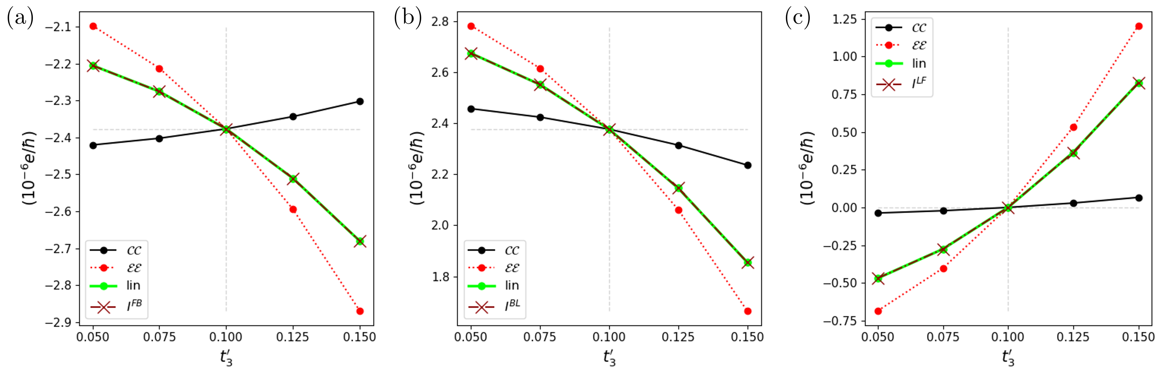
Figure 10: Plots of the (a) $I^{\text{FB}}$, (b) $I^{\text{BL}}$, (c) $I^{\text{LF}}$ hinge currents for the two-layer square plaquette model with zigzag edges versus $t^{\prime}_{3}$. The plots compare the hinge current predicted from the different local markers to the directly computed hinge current. When $t^{\prime}_{3}=0.1$ (axion-odd regime), all the markers yield the correct values of the hinge currents, as indicated by the intersections of the dashed horizontal and vertical gray lines. Generally, only the surface magnetizations found from the ‘lin’ marker always match the directly computed hinge currents.

In the axion-even regime, the markers at a single surface facet yield differing values of the magnetizations, and none except the ‘lin’ marker predict the hinge currents correctly.

These observations are highlighted in Fig. 10, which displays the hinge currents as a function of $t^{\prime}_{3}$ and compares the currents predicted using the different markers to the directly computed hinge currents.

V.3 Four-layer square plaquette model

The model studied in this section employs the same underlying square-plaquette layers that were used in Sec. V.2 and is depicted in Fig. 9(c). Just like the model of Sec. V.2, the present model features equidistantly spaced layers of the plaquette model stacked directly on top of one another along the $\hat{\textbf{z}}$ direction, but now the adjacent layers are related by a time-reversed rotation $C^{\prime}_{4z}$ about a $z$ axis passing through the C site, resulting in four layers per unit cell. The lattice vector along the stacking direction is $\textbf{a}_{3}=\hat{\textbf{z}}$. Otherwise, the models share the same features.

Table 9: Surface magnetizations and hinge currents (in units of $10^{-7}e/\hbar$) for the four-layer plaquette model with straight-edge terminations and with $t^{\prime}_{3}=0.1$ (axion-odd).

	$M_{\perp}^{\text{B}}$	$M_{\perp}^{\text{F}}$	$M_{\perp}^{\text{L}}$	$\Delta M^{\text{FB}}$	$\Delta M^{\text{BL}}$	$\Delta M^{\text{LF}}$
$M^{\cal CC}$	3.24982	0.00059	$-$0.00059	$-$3.24923	3.25040	$-$0.00117
$M^{\cal EE}$	3.24982	0.00066	$-$0.00066	$-$3.24915	3.25048	$-$0.00133
$M^{\text{lin}}$	3.24982	0.00064	$-$0.00064	$-$3.24918	3.25046	$-$0.00128
$I_{\text{calc}}$				$-$3.24918	3.25046	$-$0.00128

This model features a two-fold rotation axis $C_{2x}$ between the second and third layers in the unit cell and passing above the C and D sites. There is also a $\{C_{2z}|c/2\}$ screw axis that passes through the C sites. Together these symmetries eliminate the bulk magnetization. If the interlayer hoppings $t_{3}$ and $t^{\prime}_{3}$ are equal, the model gains an additional axion-odd $\{C^{\prime}_{4z}|c/4\}$ screw axis running through the C sites. All parameters except $t^{\prime}_{3}$ are kept fixed in order to access the quantized CSA coupling regime. We employ the same values of the parameters as in Sec. V.2, but here we set the onsite energy $\Delta=-1$.

For this model, we also study the behavior of hinge currents and surface magnetizations for the different transverse surface terminations.

V.3.1 Four-layer plaquette model: straight edges

The magnetizations $M^{\text{B}}_{\perp}$, $M^{\text{F}}_{\perp}$, and $M^{\text{L}}_{\perp}$ are found from slabs with six unit cells along $\textbf{a}_{3}$, four unit cells along $\textbf{a}_{2}$, and four unit cells along $\textbf{a}_{1}$, respectively. For each magnetization, a $7\times 7$ k-space mesh in reduced coordinates is used.

Table 10: Surface magnetizations and hinge currents (in units of $10^{-7}e/\hbar$) for the four-layer plaquette model with straight-edge terminations and with $t^{\prime}_{3}=0.15$ (axion-even).

	$M_{\perp}^{\text{B}}$	$M_{\perp}^{\text{F}}$	$M_{\perp}^{\text{L}}$	$\Delta M^{\text{FB}}$	$\Delta M^{\text{BL}}$	$\Delta M^{\text{LF}}$
$M^{\cal CC}$	3.22067	0.01107	0.00912	$-$3.20960	3.21155	$-$0.00195
$M^{\cal EE}$	3.22047	0.01130	0.00910	$-$3.20916	3.21137	$-$0.00221
$M^{\text{lin}}$	3.22053	0.01123	0.00911	$-$3.20931	3.21143	$-$0.00212
$I_{\text{calc}}$				$-$3.20931	3.21143	$-$0.00212

The macroscopic hinge current $I^{\text{FB}}$ is found using an $x$-extensive rod composed of six unit cells along $\textbf{a}_{3}$ and four unit cells along $\textbf{a}_{2}$. The $y$-extensive rod employed for $I^{\text{BL}}$ is composed of six unit cells along $\textbf{a}_{3}$ and four unit cells along $\textbf{a}_{1}$, while the $z$-extensive rod for $I^{\text{LF}}$ is composed of four unit cells along both $\textbf{a}_{1}$ and $\textbf{a}_{2}$. For each rod, a 1D k-space sampling of thirty points is employed.

For $t^{\prime}_{3}=0.1$ and $t^{\prime}_{3}=0.15$, respectively, Tables 9 and 10 report the values of the surface magnetizations computed from the different markers. In the axion-odd regime when $t^{\prime}_{3}=0.1$, all markers yield the same value for one of the surface magnetizations, namely $M_{\perp}^{\text{B}}$. This time, however, for both $M_{\perp}^{\text{F}}$ and $M_{\perp}^{\text{L}}$, the markers yield different values. Moreover, only the ‘lin’ marker accurately predicts the hinge currents. For each marker, the values for $M_{\perp}^{\text{F}}$ and $M_{\perp}^{\text{L}}$ are equal and opposite, which may be understood to be a consequence of the $\{C^{\prime}_{4z}|c/4\}$ screw symmetry, see Fig. 4(b). Nevertheless, we now have a case where the markers disagree, and where only one of them correctly predicts the hinge currents.

Table 11: Surface magnetizations and hinge currents (in units of $10^{-7}e/\hbar$) for the four-layer plaquette model with zigzag terminations and with $t^{\prime}_{3}=0.1$ (axion-odd).

	$M_{\perp}^{\text{B}}$	$M_{\perp}^{\text{F}}$	$M_{\perp}^{\text{L}}$	$\Delta M^{\text{FB}}$	$\Delta M^{\text{BL}}$	$\Delta M^{\text{LF}}$
$M^{\cal CC}$	3.24982	0.00000	0.00000	$-$3.24982	3.24982	0.00000
$M^{\cal EE}$	3.24982	0.00000	0.00000	$-$3.24982	3.24982	0.00000
$M^{\text{lin}}$	3.24982	0.00000	0.00000	$-$3.24982	3.24982	0.00000
$I_{\text{calc}}$				$-$3.24982	3.24982	0.00000

The same is true in the axion-even regime of Table 10. Fig. 11 demonstrates these facts for the prediction of the $I^{\text{LF}}$ hinge current. For all the values of $t^{\prime}_{3}$ that we used, covering both axion-odd and axion-even regimes, only the ‘lin’ marker was consistent in its prediction of the current.

V.3.2 Four-layer plaquette model: zigzag edges

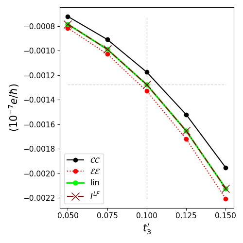
Figure 11: Plot of the hinge current $I^{\text{LF}}$ as a function of $t^{\prime}_{3}$ for the four-layer square plaquette model with straight edges. In the axion-odd regime when $t^{\prime}_{3}=0.1$, only the ‘lin’ marker correctly predicts the hinge current; this is also the case even when no axion-odd symmetry is present.

As in the case of two-layer plaquette model with zigzag terminations in Sec. V.2.2, we turn to using the supercell vectors $\textbf{A}_{1}=\textbf{a}_{1}-\textbf{a}_{2}$, $\textbf{A}_{2}=\textbf{a}_{1}+\textbf{a}_{2}$, and $\textbf{A}_{3}=\textbf{a}_{3}$ for our calculations involving the zigzag edges of the four-layer plaquette model. We align the $x$ and $y$ axes along $\textbf{A}_{1}$ and $\textbf{A}_{2}$ respectively. Since the bottom surface of a slab cut along $\textbf{A}_{3}$ is identical up to a rotation in the $x$-$y$ plane to the bottom surface of the slabs used to compute $M^{\text{B}}_{\perp}$ in the straight-edge case, the values of $M^{\text{B}}_{\perp}$ will be left unchanged. With the rotation of the coordinate axes, $C_{2x}$ becomes $C_{2xy}$. $M^{\text{F}}_{\perp}$ and $M^{\text{L}}_{\perp}$ in this case are found from slabs with three cells along $\textbf{A}_{2}$ and $\textbf{A}_{1}$, respectively. For each magnetization, a $5\times 5$ k-space mesh is used in reduced coordinates.

The macroscopic hinge current $I^{\text{FB}}$ is found from an $x$-extensive rod composed of four unit cells along $\textbf{A}_{3}$ and six unit cells along $\textbf{A}_{2}$. The $y$-extensive rod employed for $I^{\text{BL}}$ is composed of four unit cells along $\textbf{A}_{3}$ and six unit cells along $\textbf{A}_{1}$, while the $z$-extensive rod for $I^{\text{LF}}$ is composed of six cells along both $\textbf{A}_{1}$ and $\textbf{A}_{2}$. For each rod, a 1D k-space sampling of 5 points is employed.

Tables 11 and 12 report the values of the surface magnetizations computed from the different markers for $t^{\prime}_{3}=0.1$ and $t^{\prime}_{3}=0.15$, respectively. This time, in the axion-odd regime when $t^{\prime}_{3}=0.1$, we see that for any given surface facet, all markers yield the same value of magnetization, and when compared across facets, all accurately predict the hinge currents. The values of $M_{\perp}^{\text{F}}$ and $M_{\perp}^{\text{L}}$ vanish, which may be understood to be a consequence of the simultaneous $C_{2xy}$ and $\{C^{\prime}_{4z}|c/4\}$ symmetries. The former symmetry implies that $M_{\perp}^{\text{F}}=M_{\perp}^{\text{L}}$, while the latter results in both vanishing.

Table 12: Surface magnetizations and hinge currents (in units of $10^{-7}e/\hbar$) for the four-layer plaquette model with zigzag terminations and with $t^{\prime}_{3}=0.15$ (axion-even).

	$M_{\perp}^{\text{B}}$	$M_{\perp}^{\text{F}}$	$M_{\perp}^{\text{L}}$	$\Delta M^{\text{FB}}$	$\Delta M^{\text{BL}}$	$\Delta M^{\text{LF}}$
$M^{\cal CC}$	3.22067	0.01023	0.01023	$-$3.21045	3.21045	0.00000
$M^{\cal EE}$	3.22047	0.01033	0.01033	$-$3.21014	3.21014	0.00000
$M^{\text{lin}}$	3.22053	0.01029	0.01029	$-$3.21024	3.21024	0.00000
$I_{\text{calc}}$				$-$3.21024	3.21024	0.00000

In the axion-even regime when $t^{\prime}_{3}=0.15$, we find a result that is more reminiscent of the straight-edge case. That is, even for a single surface facet, the markers yield different values of the magnetization, and the hinge currents computed from the differences of $M_{\perp}$ values disagree with each other when computed using different markers. They also disagree with the direct calculation of the hinge current except for one case, namely that of the $\mathcal{M}^{\text{lin}}$ marker. $M^{\text{F}}_{\perp}$ and $M^{\text{L}}_{\perp}$ are found to be identical, as the $C_{2xy}$ symmetry is still present in this setup. However, only the $\mathcal{M}^{\text{lin}}$ marker yields magnetizations that correctly predict the hinge currents.

V.3.3 Summary

For the four-layer plaquette model, unlike the models studied previously, we find that different markers generally disagree on the values of $M_{\perp}$ and on their predictions for the hinge currents. This occurs in both the axion-odd and axion-even cases for straight-edge surface terminations, but only in the axion-even case for zigzag surface terminations. Only the $\mathcal{M}^{\text{lin}}$ marker consistently predicts the correct hinge currents.

Table 13: Diagonal elements of the traceless marker-based MQMs compared to the MQM from the current-based formula. Only the MQM derived from the $\mathcal{M}^{\text{lin}}$ marker matches the current based quadrupole. Entries are in units of $e/\hbar$.

	$Q_{xx}$	$Q_{yy}$	$Q_{zz}$
$\cal CC$	$-9.9765\times 10^{-3}$	$-9.9765\times 10^{-3}$	$1.9953\times 10^{-2}$
$\cal EE$	$-1.2540\times 10^{-2}$	$-1.2540\times 10^{-2}$	$2.5079\times 10^{-2}$
lin	$-1.1685\times 10^{-2}$	$-1.1685\times 10^{-2}$	$2.3370\times 10^{-2}$
Curr.	$-1.1685\times 10^{-2}$	$-1.1685\times 10^{-2}$	$2.3370\times 10^{-2}$

V.4 Local markers and magnetic quadrupole moment of a finite system

We now return to investigate the questions posed in Sec. IV.1.4 by conducting a numerical study of a spinless TB model of a cubic “molecule”. The system is designed to have a symmetry that enforces a vanishing magnetic dipole moment, but otherwise is as arbitrary as possible. In particular, it has no axion-odd symmetries. The structure, TB site labeling, and onsite energies of the model are depicted in Fig. 12. Additionally, the model features hoppings $t_{ij}$ to nearest, second-nearest, and third-nearest neighbors, where the subscripts indicate a hopping from TB site $i$ to TB site $j$. The hoppings are generally complex with $t_{ij}=t^{*}_{ji}$ to ensure that the Hamiltonian is Hermitian.

Table 14: Off diagonal elements of the traceless marker-based MQMs compared to the MQM from the current-based formula. Only the MQM derived from the $\mathcal{M}^{\text{lin}}$ marker matches the current-based quadrupole. Entries are in units of $e/\hbar$.

	$Q_{xy}$	$Q_{yx}$
$\cal CC$	$-6.4152\times 10^{-2}$	$6.4152\times 10^{-2}$
$\cal EE$	$-8.4555\times 10^{-2}$	$8.4555\times 10^{-2}$
lin	$-7.7754\times 10^{-2}$	$7.7754\times 10^{-2}$
Curr.	$-7.7754\times 10^{-2}$	$7.7754\times 10^{-2}$

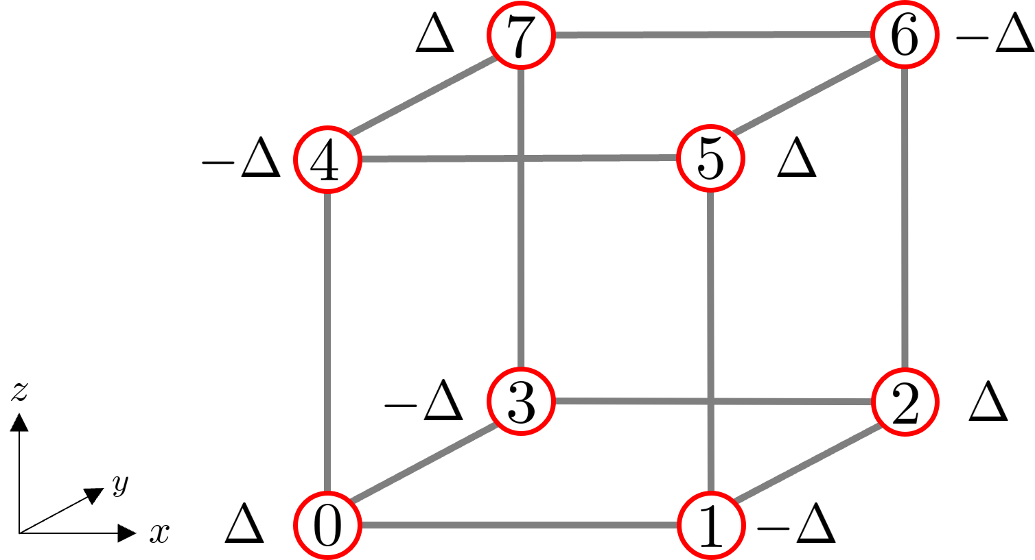
Figure 12: Illustration of the structure, labeling, and onsite energies of the cubic molecule model discussed in Sec. V.4.

The Hamiltonian is chosen to obey an $S^{\prime}_{4z}=m_{z}C^{\prime}_{4z}$ improper rotation symmetry, where the $m_{z}$ mirror plane bisects the molecule, while the $C^{\prime}_{4z}$ axis runs through the center of the cube. The resulting magnetic point group of the system is then $\{E,S^{\prime}_{4z},(S^{\prime}_{4z})^{-1},C_{2z}\}$, where $E$ is the identity operation and $C_{2z}$ is the square of $S^{\prime}_{4z}$. These symmetries ensure a vanishing magnetic dipole moment, resulting in an origin-independent, physically meaningful MQM for the system. The magnetic point group also ensures that the MQM features $Q_{xx}=Q_{yy}$ and $Q_{xy}=-Q_{yx}$. Additionally, $Q_{zz}=-2Q_{xx}$, as the tensor is traceless.

In addition to the onsite energies, the Hamiltonian is parametrized by eight hopping parameters. The nearest neighbor hopping terms $t_{1}$, $t_{2}$, and $t_{3}$ parametrize, respectively, the hoppings

$$t_{10}=t_{56}=t_{32}=t_{74},$$

$$t_{30}=t_{54}=t_{12}=t_{76},$$

$$t_{40}=t_{51}=t_{62}=t_{73}.$$

The second nearest neighbor hopping terms $t_{4}$, $t_{5}$, $t_{6}$, and $t_{7}$ parametrize the hoppings

$$t_{20} = t_{57},$$

$$t_{31} = t_{64},$$

$$t_{50} = t_{52}=t_{72}=t_{70},$$

$$t_{14} = t_{16}=t_{36}=t_{34},$$

respectively. Finally, the third nearest neighbor hopping $t_{8}$ parametrizes the hoppings $t_{35}=t_{17}=t_{24}=t_{06}$.

Generally, the hopping parameters are set to be complex, but due to the presence of the $C_{2z}$ symmetry in the magnetic point group, $t_{4}$ and $t_{5}$ must be real. The parameters for this model are chosen as $\Delta=-1$, $t_{1}=1+0.2i$, $t_{2}=1+0.3i$, $t_{3}=1-0.1i$, $t_{4}=-0.3$, $t_{5}=0.5$, $t_{6}=-0.2+0.15i$, $t_{7}=0.3-0.25i$, and $t_{8}=0.4+0.6i$.

We then calculate the current-based quadrupole and the traceless dipole-based quadrupoles based on the $\mathcal{CC}$, $\mathcal{EE}$ and ‘lin’ markers. Table 13 lists the results for diagonal elements of the quadrupoles, while Table 14 lists the nonzero off diagonal elements. We see that all feature $Q_{xx}=Q_{yy}=-Q_{zz}/2$ and $Q_{xy}=-Q_{yx}$ as expected. Significantly, though, only the $\mathcal{M}^{\text{lin}}$ marker generates a quadrupole that matches the current-based MQM.

VI Discussion

The results presented above help us to address the main questions motivating this work. First, does the introduction of quantum mechanics in the form of a marker-based theory provide a prescription for computing $M_{\perp}$ directly for a given facet, in such a way that hinge currents at adjoining facets are correctly predicted? Is this equally true in the axion-odd and axion-even cases? Second, if multiple markers succeed in doing so, does the quantum theory inherit the shift freedom of the classical theory? The most simplistic scenario would be one in which all of the physically acceptable markers identified at the end of Sec. IV.1 yield identical $M_{\perp}$ values for any given facet over all models, and correctly predict the hinge currents where facets meet.

Focusing first on the axion-odd case, we found that our tests were consistent with this simplistic scenario for the alternating Haldane and two-layer square-plaquette models. However, the four-layer square-plaquette model does show signs of trouble. For the straight-edge surface terminations, the magnetizations found from the $\mathcal{M}^{\mathcal{C},\mathcal{C}}$, $\mathcal{M}^{\mathcal{E},\mathcal{E}}$, and $\mathcal{M}^{\text{lin}}$ markers do not agree with each other. Furthermore, among these, we found that only the $\mathcal{M}^{\text{lin}}$ marker correctly predicts the hinge current. Thus, while the physical magnetization is uniquely defined in the axion-odd case, only the $\mathcal{M}^{\text{lin}}$ marker consistently gives the correct value for it in our tests.

When tuning from the axion-odd to the axion-even regime, the same conclusion was reinforced. While all markers continued to agree with each other for the stacked Haldane model, they disagreed in all other cases, i.e., for the two-layer square-plaquette model and all surface terminations of the four-layer square-plaquette model. Again, the only marker that always reproduced the hinge currents across all models was the $\mathcal{M}^{\text{lin}}$ marker.

The importance of the $\mathcal{M}^{\text{lin}}$ marker was also highlighted by our numerical finding that the dipole-based traceless MQM derived from it appears to correctly reproduce the current-based MQM in finite systems. Thus, we provisionally identify $M^{\mathrm{lin}}$ as the best candidate for a marker-based formulation of a theory of surface orbital magnetization.

Given the $\mathcal{M}^{\text{lin}}$ marker’s evident connection to the MQM, we have also explored the symmetries of our models to understand whether they permit a nonzero bulk MQM. While the question of defining an orbital MQM for a general bulk material has received some attention Shitade et al. (2018); Gao and Xiao (2018), the situation appears to remain unsettled. Assuming such a definition is possible, however, it must respect the symmetries of the magnetic point group.

The four-layer square-plaquette model is most informative in this respect. Focusing first on the axion-odd case, the tensor is diagonal with $Q_{xx}=-Q_{yy}$ nonzero and $Q_{zz}=0$ when the coordinate axes are chosen as in Fig. 9(c) for the straight-edge surfaces. In the zigzag-edge case, we rotated the axes about $\hat{\textbf{z}}$ by $-\pi/4$, transforming the tensor such that the only nonzero elements were $Q^{\prime}_{xy}=Q^{\prime}_{yx}$. We found that the markers disagreed with each other in precisely those cases in which the corresponding diagonal MQM tensor element was nonzero, namely for the side surfaces in the straight-edge case. According to Eq. (34), these were also the cases in which the bulk MQM has the right symmetry to contribute to the surface magnetization. When the axion-odd symmetry was broken, we found that all three diagonal elements were present in the MQM for both surface terminations, and that the markers disagreed with each other for all surfaces

For the alternating Haldane and two-layer square-plaquette models, the symmetry of the MQM is such that it vanishes in the axion-odd regime but acquires some diagonal elements in the axion-even regime. For the latter model, the markers also failed to agree in the axion-even regime.

To summarize our discussion of the numerical results, when inspecting all three models, we found that the only cases in which markers disagree, with only the $\mathcal{M}^{\text{lin}}$ marker correctly predicting the hinge currents, were those in which diagonal elements of the MQM tensor were present. Thus, however the bulk MQM might be defined, our results suggest that only the $\mathcal{M}^{\text{lin}}$ marker accurately takes into account its contribution to surface magnetization.

Notably, our findings provide no evidence for the possible marker shift freedom of the surface magnetizations within the quantum-mechanical marker-based theory. In fact, since only the $\mathcal{M}^{\text{lin}}$ marker always yielded the correct hinge currents, we do not have multiple marker candidates as would be be needed to allow us to test this proposition.

We find ourselves, then, in a somewhat ambiguous position. Our empirical evidence, based on the model studies, indicates that the original Bianco-Resta marker $\mathcal{M}^{\mathcal{C,C}}$ is not suitable for coarse-graining to obtain the surface magnetization. Instead, a modification of it, namely $\mathcal{M}^{\mathrm{lin}}$, has passed all tests and appears to be a suitable marker. Still, despite a concerted effort to find a formal connection, we do not yet have a fundamental understanding as to why $M^{\mathrm{lin}}$ succeeds where the others do not. It also cannot yet be ruled out that $M^{\mathrm{lin}}$ does not pass all tests in models beyond those considered in this paper. Our work thus raises these issue as being of paramount importance to be addressed by future theoretical investigations.

We now also comment in more detail on the connection of this work to that of Zhu et al. Zhu et al. (2021). The authors of that work also introduced the notion of surface orbital magnetization, and similarly used the local marker formulation of orbital magnetism to compute it. Their primary focus, as we mentioned just before Sec. IV.1.1, was to explore the “facet magnetic compressibility” $dM_{\perp}/d\mu$ that is directly proportional to the geometric component of the surface AHC, especially in the context of links to higher-order topology. We agree with their conclusion that this compressibility is uniquely determined. On the other hand, where they assumed that the Bianco-Resta $\mathcal{M}^{\mathcal{C,C}}$ marker could be applied to define surface magnetization, our findings indicate that this assumption was problematic. We also note that they did not explore the issue of a possible shift freedom of the surface magnetization.

Of course, it would be desirable to make contact with experiment. We have argued that the hinge currents are observable in principle via the magnetic fields they generate, which could be observed by scanning magnetic probes. The surface magnetization $M_{\perp}$ itself in the interior of a facet does not produce any observable electric or magnetic potential, and so cannot be observed directly. It is possible that optical probes, such as terahertz Kerr reflectivity, might provide information. However, one should keep in mind that when symmetry allows for the presence of a surface orbital magnetization, it also allows for a surface spin magnetization, which is likely to be much larger. Thus, filtering out just the orbital component may be challenging.

Other generalizations of our present work remain to be developed. The symmetry analysis of Sec. III was conducted in full generality and is applicable to insulating as well as metallic systems at any temperature. However, it is not immediately clear whether it is possible to compute surface magnetization using the local marker for $T\neq 0$. A crucial assumption going into the construction of the local marker is the idempotency of $P$ Bianco and Resta (2013); in the case of finite temperature, $P$ no longer displays this behavior. Additionally, for metals at $T=0$, even though $P$ remains idempotent, it is no longer exponentially localized, with $P(\textbf{r},\textbf{r}^{\prime})$ featuring power law decay with $|\textbf{r}-\textbf{r}^{\prime}|$. It is not immediately clear how this affects the local marker and its subsequent coarse-grained average. In these situations, it appears likely that a different method of computing surface magnetization will be needed. We note, however, that prior numerical tests performed on TB models of metals at $T=0$ suggest that the local marker is able to reproduce the bulk magnetization of Eq. (1) within open boundary conditions, but exhibits slower convergence with sample size than in the insulating case Marrazzo and Resta (2016).

Additional directions to explore include the presence of facet magnetizations for systems with bulk magnetization, as well as for axion-odd systems with $\theta_{\text{CS}}=\pi$. It would also be interesting to see whether a Wannier-based formulation for surface magnetization is possible, at least in insulators. This is particularly attractive as the theories of bulk electric polarization, bulk orbital magnetization, and edge electric polarization can all be developed using a Wannier-based approach King-Smith and Vanderbilt (1993); Vanderbilt and King-Smith (1993); Thonhauser et al. (2005); Ceresoli et al. (2006); Ren et al. (2021); Trifunovic (2020). Finally, we mention the prospects for a first-principles density-functional theory (DFT) implementation of the calculation of surface magnetization for topologically trivial bulk materials. The output of any DFT calculation may be adapted to a TB framework via Wannier interpolation, which may be accomplished by code packages such as Wannier90 Pizzi et al. (2020). It is important to keep in mind, however, that in our calculations of the local markers we employed the diagonal approximation for the position operator. In the case of a Wannier interpolation, the position operator is not necessarily diagonal in the basis of Wannier states, and the off-diagonal terms must be kept in mind when performing calculations.

VII Summary

In this work, we have explored the possibility of defining surface orbital magnetization for insulating systems that are topologically trivial in the bulk and feature no bulk orbital magnetization. We have demonstrated that in a general classical context, the knowledge of the macroscopic currents residing on a hinge formed by two surface facets is sufficient to determine only the difference of the magnetizations of the two facets. The said macroscopic hinge currents are the physical observables corresponding to the presence of surface orbital magnetization, and this fact indicates that differences of surface orbital magnetization are observables as well. By means of a symmetry analysis, we have shown that individual values of facet magnetizations should be well defined when the bulk symmetry group contains an axion-odd symmetry. To develop the theory of surface magnetization in a quantum context, we further expanded on the local marker formulation of orbital magnetization developed by Bianco and Resta, and introduced a set of markers satisfying a list of physically meaningful transformation requirements. The coarse-grained averages of these markers were then used to compute surface magnetizations.

We tested the conclusions of our symmetry analysis and our formalism for computing surface magnetization on a series of spinless TB models. We found that the markers do not always agree on the value of the surface magnetization, even in the axion-odd case where we know from symmetry arguments that $M_{\perp}$ is well defined. Our results indicate that only a single marker on our list, the $\mathcal{M}^{\text{lin}}$ marker, consistently predicts the correct hinge currents. According to the symmetry considerations of Sec. III, in the axion-odd case we can then conclude that it has correctly computed the unique $M_{\perp}$ values. In the axion-even case, instead, we can no longer say that it predicts uniquely correct $M_{\perp}$ values, only correct differences of $M_{\perp}$ values.

We additionally tested the markers to understand whether any of them correctly generated the current-based MQM of Eq. (31), which we argued may contribute to surface magnetization. We found that only the $\mathcal{M}^{\text{lin}}$ marker correctly reproduced the current-based MQM when applied to a finite system with a nontrivial MQM and vanishing magnetic dipole moment. We also observed that when the different markers failed to agree on the surface magnetizations for axion-odd systems, the bulk symmetry group permitted an MQM that could contribute to the surface magnetizations.

Overall, our study indicates that a coarse-graining of the $\mathcal{M}^{\text{lin}}$ marker provides a suitable framework for computing surface magnetizations. However, a formal derivation that would explain the unique success of the $\mathcal{M}^{\text{lin}}$ marker remains elusive, and questions persist about the definition and role of the bulk quadrupole tensor. Thus, while our work establishes a foundation for a theory of surface orbital magnetization, it also highlights the need for further work to resolve some important remaining questions.

Note added: After submission of this paper, we became aware of a subsequent preprint by Gliozzi, Lin and Hughes Gliozzi et al. (2022) that also considers, though from a different perspective, issues related to surface orbital magnetization, hinge currents, and bulk magnetic quadrupole moments.

Appendix A Local marker for slab geometries in the tight-binding representation

In this Appendix, we provide further exposition on the calculation of the local markers in the context of TB models. For concreteness, we will focus on computing the marker for insulating slabs that are of sufficient finite thickness in the $z$ direction, but infinite in-plane, as in Sec. IV.2.

The $\mathcal{M}^{\mathcal{C},\mathcal{C}}$, $\mathcal{M}^{\mathcal{E},\mathcal{E}}$, and $\mathcal{M}^{\text{lin}}$ local markers for the magnetization are all expressible in terms of the LC local markers of Eqs. (20-22) and their IC marker analogues. In this Appendix, we restrict ourselves to a calculation of the marker of Eq. (20), which for a TB site $i$ is given by

$$\mathcal{M}^{\mathcal{C}}_{\text{LC}}(i)=-\frac{e}{\hbar}\text{Im}\langle i|XHY^{\dagger}|i\rangle.$$ (48)

The calculations for all other LC and IC markers are similar, and we will simply state the results at the end of this Appendix.

We remind the reader that in all of our models, we have set the Fermi energy inside the band gap at zero, so that we ignore the Chern marker contribution to the local marker. For details on how to compute the Chern marker in the TB representation, we refer the reader to Ref. Varnava and Vanderbilt (2018).

We denote the valence ($v$) and conduction ($c$) band eigenstates of the slab Hamiltonian as $\psi_{v\textbf{k}}(\textbf{r})$ and $\psi_{c\textbf{k}}(\textbf{r})$, respectively, where $\textbf{k}=(k_{x},k_{y})$. The valence and conduction band projectors are then written as $P=(1/N_{\textbf{k}})\sum_{v\textbf{k}}|\psi_{v\textbf{k}}\rangle\langle\psi_{v\textbf{k}}|$ and $Q=(1/N_{\textbf{k}})\sum_{c\textbf{k}}|\psi_{c\textbf{k}}\rangle\langle\psi_{c\textbf{k}}|$, where $N_{\textbf{k}}$ is the number of k points in the 2D Brillouin zone mesh. With this in mind, we observe that

$$\mathcal{M}^{\mathcal{C}}_{\text{LC}}(i) =-\frac{e}{\hbar}\text{Im}\langle i|XHY^{\dagger}|i\rangle$$

$$=-\frac{e}{N_{\textbf{k}}\hbar}\text{Im}\sum_{\textbf{k}}\sum_{vv^{\prime}cc^{\prime}}\langle i|\psi_{v\textbf{k}}\rangle\langle\psi_{v\textbf{k}}|x|\psi_{c\textbf{k}}\rangle\langle\psi_{c\textbf{k}}|H|\psi_{c^{\prime}\textbf{k}}\rangle\langle\psi_{c^{\prime}\textbf{k}}|y|\psi_{v^{\prime}\textbf{k}}\rangle\langle\psi_{v^{\prime}\textbf{k}}|i\rangle$$

$$=-\frac{e}{N_{\textbf{k}}\hbar}\text{Im}\sum_{\textbf{k}}\sum_{vv^{\prime}c}E_{c\textbf{k}}\psi_{v\textbf{k}}(i)\psi^{*}_{v^{\prime}\textbf{k}}(i)X_{vc\textbf{k}}Y^{\dagger}_{cv^{\prime}\textbf{k}},$$ (49)

where $E_{n\textbf{k}}$ is the eigenenergy corresponding to $|\psi_{n\textbf{k}}\rangle$, $X_{vc\textbf{k}}=\langle\psi_{v\textbf{k}}|x|\psi_{c\textbf{k}}\rangle$, and $Y^{\dagger}_{cv\textbf{k}}=\langle\psi_{c\textbf{k}}|y|\psi_{v\textbf{k}}\rangle$.

In our calculations of the local markers, we do not directly compute the matrix elements of the position operators $x$ and $y$ in the energy eigenbasis; rather, we use the velocity operator $\hat{\textbf{v}}$, defined as

$$\hat{\textbf{v}}=\frac{1}{i\hbar}[\hat{\textbf{r}},H],$$ (50)

to rewrite

$$X_{vc\textbf{k}}=\frac{\langle\psi_{v\textbf{k}}|i\hbar v_{x}|\psi_{c\textbf{k}}\rangle}{E_{c\textbf{k}}-E_{v\textbf{k}}}$$ (51)

and similarly for $Y^{\dagger}_{cv^{\prime}\textbf{k}}$.

The three LC markers are then

$$\mathcal{M}^{\mathcal{C}}_{\text{LC}}(i)=-\frac{e}{N_{\textbf{k}}\hbar}\text{Im}\sum_{\textbf{k}}\sum_{vv^{\prime}c}E_{c\textbf{k}}\psi_{v\textbf{k}}(i)\psi^{*}_{v^{\prime}\textbf{k}}(i)X_{vc\textbf{k}}Y^{\dagger}_{cv^{\prime}\textbf{k}},$$ (52)

$$\mathcal{M}^{\mathcal{L}}_{\text{LC}}(i)=-\frac{e}{N_{\textbf{k}}\hbar}\text{Im}\sum_{\textbf{k}}\sum_{cc^{\prime}v}E_{c\textbf{k}}\psi_{c\textbf{k}}(i)\psi^{*}_{c^{\prime}\textbf{k}}(i)X_{vc^{\prime}\textbf{k}}Y^{\dagger}_{cv\textbf{k}},$$ (53)

$$\mathcal{M}^{\mathcal{R}}_{\text{LC}}(i)=-\frac{e}{N_{\textbf{k}}\hbar}\text{Im}\sum_{\textbf{k}}\sum_{cc^{\prime}v}E_{c^{\prime}\textbf{k}}\psi_{c\textbf{k}}(i)\psi^{*}_{c^{\prime}\textbf{k}}(i)X_{vc^{\prime}\textbf{k}}Y^{\dagger}_{cv\textbf{k}}.$$ (54)

The three IC markers are

$$\mathcal{M}^{\mathcal{C}}_{\text{IC}}(i)=\frac{e}{N_{\textbf{k}}\hbar}\text{Im}\sum_{\textbf{k}}\sum_{cc^{\prime}v}E_{v\textbf{k}}\psi_{c\textbf{k}}(i)\psi^{*}_{c^{\prime}\textbf{k}}(i)X^{\dagger}_{cv\textbf{k}}Y_{vc^{\prime}\textbf{k}},$$ (55)

$$\mathcal{M}^{\mathcal{L}}_{\text{IC}}(i)=\frac{e}{N_{\textbf{k}}\hbar}\text{Im}\sum_{\textbf{k}}\sum_{vv^{\prime}c}E_{v\textbf{k}}\psi_{v\textbf{k}}(i)\psi^{*}_{v^{\prime}\textbf{k}}(i)X^{\dagger}_{cv^{\prime}\textbf{k}}Y_{vc\textbf{k}},$$ (56)

$$\mathcal{M}^{\mathcal{R}}_{\text{IC}}(i)=\frac{e}{N_{\textbf{k}}\hbar}\text{Im}\sum_{\textbf{k}}\sum_{vv^{\prime}c}E_{v^{\prime}\textbf{k}}\psi_{v\textbf{k}}(i)\psi^{*}_{v^{\prime}\textbf{k}}(i)X^{\dagger}_{cv^{\prime}\textbf{k}}Y_{vc\textbf{k}}.$$ (57)

The combinations of these markers then yield the $\mathcal{M}^{\mathcal{C},\mathcal{C}}$, $\mathcal{M}^{\mathcal{E},\mathcal{E}}$, and $\mathcal{M}^{\text{lin}}$ markers.

Appendix B Microscopic tight-binding currents

Here, we give further details on the calculation of the microscopic current density in the TB representation. Our derivation in Sec. IV.3 was centered on continuum models, and we briefly noted that in a TB context Eq. (46) turns into a discrete sum over TB sites.

Due to the discrete nature of TB models, microscopic currents are more naturally defined along straight-line paths, which we refer to as bonds, between different TB sites, rather than at individual TB sites. Assuming that each TB site hosts a single orbital (the generalization to the multi-orbital case being straightforward), the bond current between TB sites $i$ and $j$ arises from the probabilities for a particle to hop from site $i$ to site $j$ and vice-versa. Recall from the introduction to Sec. V that we have adopted a diagonal approximation to the matrix elements of the position operators in the TB basis,

$$\langle i|\hat{\textbf{r}}|j\rangle=\textbf{r}_{i}\delta_{ij},$$ (58)

where $\textbf{r}_{i}$ denotes the position of TB orbital $i$. With this approximation in mind, the matrix elements of the velocity operator $\hat{\textbf{v}}=(1/i\hbar)[\hat{\textbf{r}},H]$ in the TB basis are expressed as

$$\langle i|\hat{\textbf{v}}|j\rangle=\frac{1}{i\hbar}(\textbf{r}_{i}-\textbf{r}_{j})\langle i|H|j\rangle.$$ (59)

Given a set of occupied states $|\psi_{n}\rangle$, the total current in the system is given by

$$\textbf{J}=\sum^{\text{occ}}_{n}\langle\psi_{n}|\hat{\textbf{J}}|\psi_{n}\rangle$$ (60)

where $\hat{\textbf{J}}=e\hat{\textbf{v}}$ is the total current operator. Inserting resolutions of the identity in terms of the TB sites on either side of $\hat{\textbf{J}}$, we get

$$\textbf{J}=e\sum^{\text{occ}}_{n}\sum_{ij}\langle\psi_{n}|i\rangle\langle i|\hat{\textbf{v}}|j\rangle\langle j|\psi_{n}\rangle=e\sum_{ij}\langle j|P|i\rangle\langle i|\hat{\textbf{v}}|j\rangle$$ (61)

where $P$ is the ground state projector. Substituting Eq. (59), this can be written as

$$\textbf{J}=\sum_{\langle ij\rangle}\textbf{J}_{\langle ij\rangle}$$ (62)

where the sum runs over distinct pairs $\langle ij\rangle$ of sites and

$$\textbf{J}_{\langle ij\rangle}=\frac{2e}{\hbar}(\textbf{r}_{i}-\textbf{r}_{j})\text{Im}[\langle j|P|i\rangle\langle i|H|j\rangle]$$ (63)

describes the total current flowing on the bond $\langle ij\rangle$.

Since the current is assumed to flow uniformly along the straight-line bond connecting the sites, it makes no difference if we treat it as distributed uniformly along the length, concentrated at the center, or partitioned between the two end points of the bond. We make the last choice in order to write the total current as a sum over sites, $\textbf{J}=\sum_{i}\textbf{j}_{i}$, where

$$\textbf{j}_{i}=\frac{1}{2}\sum_{j}\textbf{J}_{\langle ij\rangle}.$$ (64)

We treat this as the discrete analog of Eq. (46), and we use it in the calculations of the macroscopic hinge currents in our TB models by performing the coarse-graining procedure of Sec. IV.3 on the $\textbf{j}_{i}$.

Finally, we note that in the case of the extended rod geometries used to find the macroscopic hinge currents in the main text, the valence projector $P$ is written in terms of the rod valence eigenstates $\psi_{vk}$ as $P=(1/N_{k})\sum_{vk}|\psi_{vk}\rangle\langle\psi_{vk}|$, where the sum is over the $N_{k}$ points of the mesh spanning the 1D Brillouin zone. This expression for $P$ is then substituted into Eq. (63).

Appendix C Point-dipole-based magnetic quadrupole moment

We now present a proof of Eq. (37) of the main text. Consider a collection of point magnetic dipoles $\textbf{m}_{\mu}$ located at positions $\textbf{r}_{\mu}$. We will enumerate the dipoles with Greek letters and use Latin letters to label Cartesian indices. The microscopic current distribution $\textbf{j}(\textbf{r})$ of the collection of dipoles is

$$\textbf{j}(\textbf{r})=\nabla\times\left(\sum_{\mu}\textbf{m}_{\mu}\delta(\textbf{r}-\textbf{r}_{\mu})\right)=-\sum_{\mu}\textbf{m}_{\mu}\times\nabla\delta(\textbf{r}-\textbf{r}_{\mu}).$$ (65)

We then find that $\textbf{r}\times\textbf{j}(\textbf{r})$ in the definition of the current-based MQM (see Eq. (31)) is given by

$$(\textbf{r}\times\textbf{j})_{i}=\sum_{\mu}[r_{k}m_{\mu,k}\partial_{i}-m_{\mu,i}r_{k}\partial_{k}]\delta(\textbf{r}-\textbf{r}_{\mu})$$ (66)

in an implied sum notation. Substituting this expression into Eq. (31) and integrating by parts, we find

$$Q_{ij} =\frac{1}{3}\int d\textbf{r}\,(\textbf{r}\times\textbf{j})_{i}\,r_{j}$$

$$=\frac{1}{3}\sum_{\mu}\int d\textbf{r}\left[m_{\mu,i}\partial_{k}(r_{k}r_{j})-m_{\mu,k}\partial_{i}(r_{k}r_{j})\right]\delta(\textbf{r}-\textbf{r}_{\mu})$$

$$=\sum_{\mu}m_{\mu,i}r_{\mu,j}-\frac{1}{3}\delta_{ij}m_{\mu,k}r_{\mu,k}$$

$$=Q^{\text{dip}}_{ij}-\frac{1}{3}\delta_{ij}Q_{kk}^{\text{dip}},$$ (67)

where we use the definition of $Q^{\text{dip}}_{ij}$ introduced in Eq. (36). We have thus proved Eq. (37).

Appendix D Numerical TB model results

Each of the TB models of Sec. V features 2D layers coupled by interlayer couplings that are along the layer stacking direction. In going from one layer to the next, the couplings vary between two values denoted by $t_{3}$ and $t^{\prime}_{3}$. When $t_{3}=t^{\prime}_{3}$, the systems are found to exhibit axion-odd symmetries, and only axion-even symmetries otherwise. In each of the models, all parameters are kept fixed except for $t^{\prime}_{3}$, which is used to bring the systems into and out of the axion-odd regime. For each model, $0.05\leq t^{\prime}_{3}\leq 0.15$.

In the main text, we reported the values of the facet magnetizations $M_{\perp}^{\text{B}}$, $M_{\perp}^{\text{F}}$, and $M_{\perp}^{\text{L}}$ found from the $\mathcal{CC}$, $\mathcal{EE}$, and ‘lin’ markers. Furthermore, we found the differences of facet magnetizations at different surfaces $\Delta M^{\text{FB}}$, $\Delta M^{\text{BL}}$, and $\Delta M^{\text{LF}}$, and compared them to the values of the directly computed macroscopic hinge currents. We did this for the parameter values $t^{\prime}_{3}=0.1$ and $0.15$. In this Appendix, we report this data for $t^{\prime}_{3}=0.05$, $0.075$, and $0.125$. The values of the magnetizations and currents are subject to the same symmetry constraints in the models’ respective axion-even regimes that are described in the main text.

D.1 Alternating Haldane layers

Table 15: Surface magnetizations and hinge currents (in units of $10^{-5}e/\hbar$) for the alternating Haldane model with $t^{\prime}_{3}=0.05$ (axion-even).

	$M_{\perp}^{\text{B}}$	$M_{\perp}^{\text{F}}$	$M_{\perp}^{\text{L}}$	$\Delta M^{\text{FB}}$	$\Delta M^{\text{BL}}$	$\Delta M^{\text{LF}}$
$M^{\cal CC}$	1.8148	$-$0.0493	$-$0.0096	$-$1.8641	1.8244	0.0397
$M^{\cal EE}$	1.8148	$-$0.0493	$-$0.0096	$-$1.8641	1.8244	0.0397
$M^{\text{lin}}$	1.8148	$-$0.0493	$-$0.0096	$-$1.8641	1.8244	0.0397
$I_{\text{calc}}$				$-$1.8641	1.8244	0.0397

Table 16: Surface magnetizations and hinge currents (in units of $10^{-5}e/\hbar$) for the alternating Haldane model with $t^{\prime}_{3}=0.075$ (axion-even).

	$M_{\perp}^{\text{B}}$	$M_{\perp}^{\text{F}}$	$M_{\perp}^{\text{L}}$	$\Delta M^{\text{FB}}$	$\Delta M^{\text{BL}}$	$\Delta M^{\text{LF}}$
$M^{\cal CC}$	1.8120	$-$0.0288	$-$0.0056	$-$1.8408	1.8176	0.0232
$M^{\cal EE}$	1.8120	$-$0.0288	$-$0.0056	$-$1.8408	1.8176	0.0232
$M^{\text{lin}}$	1.8120	$-$0.0288	$-$0.0056	$-$1.8408	1.8176	0.0232
$I_{\text{calc}}$				$-$1.8408	1.8176	0.0232

Table 17: Surface magnetizations and hinge currents (in units of $10^{-5}e/\hbar$) for the alternating Haldane model with $t^{\prime}_{3}=0.125$ (axion-even).

	$M_{\perp}^{\text{B}}$	$M_{\perp}^{\text{F}}$	$M_{\perp}^{\text{L}}$	$\Delta M^{\text{FB}}$	$\Delta M^{\text{BL}}$	$\Delta M^{\text{LF}}$
$M^{\cal CC}$	1.8032	0.0372	0.0073	$-$1.7659	1.7959	$-$0.0299
$M^{\cal EE}$	1.8032	0.0372	0.0073	$-$1.7659	1.7959	$-$0.0299
$M^{\text{lin}}$	1.8032	0.0372	0.0073	$-$1.7659	1.7959	$-$0.0299
$I_{\text{calc}}$				$-$1.7659	1.7959	$-$0.0299

D.2 Two-layer plaquette model: straight edges

Table 18: Surface magnetizations and hinge currents (in units of $10^{-6}e/\hbar$) for the two-layer plaquette model with straight-edge terminations and with $t^{\prime}_{3}=0.05$ (axion-even).

	$M_{\perp}^{\text{B}}$	$M_{\perp}^{\text{F}}$	$M_{\perp}^{\text{L}}$	$\Delta M^{\text{FB}}$	$\Delta M^{\text{BL}}$	$\Delta M^{\text{LF}}$
$M^{\cal CC}$	2.4215	$-$0.0174	$-$0.0174	$-$2.4390	2.4390	0.0000
$M^{\cal EE}$	2.4224	$-$0.0179	$-$0.0179	$-$2.4403	2.4403	0.0000
$M^{\text{lin}}$	2.4221	$-$0.0178	$-$0.0178	$-$2.4399	2.4399	0.0000
$I_{\text{calc}}$				$-$2.4399	2.4399	0.0000

Table 19: Surface magnetizations and hinge currents (in units of $10^{-6}e/\hbar$) for the two-layer plaquette model with straight-edge terminations and with $t^{\prime}_{3}=0.075$ (axion-even).

	$M_{\perp}^{\text{B}}$	$M_{\perp}^{\text{F}}$	$M_{\perp}^{\text{L}}$	$\Delta M^{\text{FB}}$	$\Delta M^{\text{BL}}$	$\Delta M^{\text{LF}}$
$M^{\cal CC}$	2.4030	$-$0.0103	$-$0.0103	$-$2.4133	2.4133	0.0000
$M^{\cal EE}$	2.4035	$-$0.0106	$-$0.0106	$-$2.4141	2.4141	0.0000
$M^{\text{lin}}$	2.4033	$-$0.0105	$-$0.0105	$-$2.4138	2.4138	0.0000
$I_{\text{calc}}$				$-$2.4138	2.4138	0.0000

Table 20: Surface magnetizations and hinge currents (in units of $10^{-6}e/\hbar$) for the two-layer plaquette model with straight-edge terminations and with $t^{\prime}_{3}=0.125$ (axion-even).

	$M_{\perp}^{\text{B}}$	$M_{\perp}^{\text{F}}$	$M_{\perp}^{\text{L}}$	$\Delta M^{\text{FB}}$	$\Delta M^{\text{BL}}$	$\Delta M^{\text{LF}}$
$M^{\cal CC}$	2.3430	0.0139	0.0139	$-$2.3291	2.3291	0.0000
$M^{\cal EE}$	2.3422	0.0143	0.0143	$-$2.3280	2.3280	0.0000
$M^{\text{lin}}$	2.3425	0.0141	0.0141	$-$2.3284	2.3284	0.0000
$I_{\text{calc}}$				$-$2.3284	2.3284	0.0000

D.3 Two-layer plaquette model: zigzag edges

Table 21: Surface magnetizations and hinge currents (in units of $10^{-6}e/\hbar$) for the two-layer plaquette model with zigzag terminations and with $t^{\prime}_{3}=0.05$ (axion-even).

	$M_{\perp}^{\text{B}}$	$M_{\perp}^{\text{F}}$	$M_{\perp}^{\text{L}}$	$\Delta M^{\text{FB}}$	$\Delta M^{\text{BL}}$	$\Delta M^{\text{LF}}$
$M^{\cal CC}$	2.4215	0.0011	$-$0.0359	$-$2.4204	2.4574	$-$0.0370
$M^{\cal EE}$	2.4224	0.3247	$-$0.3605	$-$2.0977	2.7829	$-$0.6852
$M^{\text{lin}}$	2.4221	0.2168	$-$0.2523	$-$2.2053	2.6744	$-$0.4691
$I_{\text{calc}}$				$-$2.2053	2.6744	$-$0.4691

Table 22: Surface magnetizations and hinge currents (in units of $10^{-6}e/\hbar$) for the two-layer plaquette model with zigzag terminations and with $t^{\prime}_{3}=0.075$ (axion-even).

	$M_{\perp}^{\text{B}}$	$M_{\perp}^{\text{F}}$	$M_{\perp}^{\text{L}}$	$\Delta M^{\text{FB}}$	$\Delta M^{\text{BL}}$	$\Delta M^{\text{LF}}$
$M^{\cal CC}$	2.4030	0.0006	$-$0.0212	$-$2.4024	2.4242	$-$0.0218
$M^{\cal EE}$	2.4035	0.1909	$-$0.2121	$-$2.2126	2.6156	$-$0.4030
$M^{\text{lin}}$	2.4033	0.1275	$-$0.1485	$-$2.2758	2.5518	$-$0.2760
$I_{\text{calc}}$				$-$2.2758	2.5518	$-$0.2760

Table 23: Surface magnetizations and hinge currents (in units of $10^{-6}e/\hbar$) for the two-layer plaquette model with zigzag terminations and with $t^{\prime}_{3}=0.125$ (axion-even).

	$M_{\perp}^{\text{B}}$	$M_{\perp}^{\text{F}}$	$M_{\perp}^{\text{L}}$	$\Delta M^{\text{FB}}$	$\Delta M^{\text{BL}}$	$\Delta M^{\text{LF}}$
$M^{\cal CC}$	2.3430	$-$0.0007	0.0284	$-$2.3437	2.3145	0.0291
$M^{\cal EE}$	2.3422	$-$0.2518	0.2803	$-$2.5941	2.0619	0.5322
$M^{\text{lin}}$	2.3425	$-$0.1681	0.1964	$-$2.5106	2.1461	0.3645
$I_{\text{calc}}$				$-$2.5106	2.1461	0.3645

D.4 Four-layer plaquette model: straight edges

Table 24: Surface magnetizations and hinge currents (in units of $10^{-7}e/\hbar$) for the four-layer plaquette model with straight-edge terminations and with $t^{\prime}_{3}=0.05$ (axion-even).

	$M_{\perp}^{\text{B}}$	$M_{\perp}^{\text{F}}$	$M_{\perp}^{\text{L}}$	$\Delta M^{\text{FB}}$	$\Delta M^{\text{BL}}$	$\Delta M^{\text{LF}}$
$M^{\cal CC}$	3.26720	$-$0.00555	$-$0.00627	$-$3.27276	3.27348	$-$0.00072
$M^{\cal EE}$	3.26732	$-$0.00557	$-$0.00638	$-$3.27289	3.27371	$-$0.00082
$M^{\text{lin}}$	3.26728	$-$0.00556	$-$0.00635	$-$3.27284	3.27363	$-$0.00078
$I_{\text{calc}}$				$-$3.27285	3.27363	$-$0.00078

Table 25: Surface magnetizations and hinge currents (in units of $10^{-7}e/\hbar$) for the four-layer plaquette model with straight-edge terminations and with $t^{\prime}_{3}=0.075$ (axion-even).

	$M_{\perp}^{\text{B}}$	$M_{\perp}^{\text{F}}$	$M_{\perp}^{\text{L}}$	$\Delta M^{\text{FB}}$	$\Delta M^{\text{BL}}$	$\Delta M^{\text{LF}}$
$M^{\cal CC}$	3.25997	$-$0.00301	$-$0.00392	$-$3.26298	3.26388	$-$0.00091
$M^{\cal EE}$	3.26004	$-$0.00298	$-$0.00401	$-$3.26302	3.26405	$-$0.00103
$M^{\text{lin}}$	3.26002	$-$0.00299	$-$0.00398	$-$3.26301	3.26400	$-$0.00099
$I_{\text{calc}}$				$-$3.26301	3.26400	$-$0.00099

Table 26: Surface magnetizations and hinge currents (in units of $10^{-7}e/\hbar$) for the four-layer plaquette model with straight-edge terminations and with $t^{\prime}_{3}=0.125$ (axion-even).

	$M_{\perp}^{\text{B}}$	$M_{\perp}^{\text{F}}$	$M_{\perp}^{\text{L}}$	$\Delta M^{\text{FB}}$	$\Delta M^{\text{BL}}$	$\Delta M^{\text{LF}}$
$M^{\cal CC}$	3.23673	0.00527	0.00375	$-$3.23146	3.23298	$-$0.00152
$M^{\cal EE}$	3.23664	0.00541	0.00369	$-$3.23122	3.23294	$-$0.00172
$M^{\text{lin}}$	3.23667	0.00536	0.00371	$-$3.23130	3.23296	$-$0.00165
$I_{\text{calc}}$				$-$3.23130	3.23296	$-$0.00165

D.5 Four-layer plaquette model: zigzag edges

Table 27: Surface magnetizations and hinge currents (in units of $10^{-7}e/\hbar$) for the four-layer plaquette model with zigzag terminations and with $t^{\prime}_{3}=0.05$ (axion-even).

	$M_{\perp}^{\text{B}}$	$M_{\perp}^{\text{F}}$	$M_{\perp}^{\text{L}}$	$\Delta M^{\text{FB}}$	$\Delta M^{\text{BL}}$	$\Delta M^{\text{LF}}$
$M^{\cal CC}$	3.26720	$-$0.00599	$-$0.00599	$-$3.27319	3.27319	0.00000
$M^{\cal EE}$	3.26732	$-$0.00605	$-$0.00605	$-$3.27337	3.27337	0.00000
$M^{\text{lin}}$	3.26728	$-$0.00603	$-$0.00603	$-$3.27331	3.27331	0.00000
$I_{\text{calc}}$				$-$3.27331	3.27331	0.00000

Table 28: Surface magnetizations and hinge currents (in units of $10^{-7}e/\hbar$) for the four-layer plaquette model with zigzag terminations and with $t^{\prime}_{3}=0.075$ (axion-even).

	$M_{\perp}^{\text{B}}$	$M_{\perp}^{\text{F}}$	$M_{\perp}^{\text{L}}$	$\Delta M^{\text{FB}}$	$\Delta M^{\text{BL}}$	$\Delta M^{\text{LF}}$
$M^{\cal CC}$	3.25997	$-$0.00351	$-$0.00351	$-$3.26347	3.26347	0.00000
$M^{\cal EE}$	3.26004	$-$0.00354	$-$0.00354	$-$3.26358	3.26358	0.00000
$M^{\text{lin}}$	3.26002	$-$0.00353	$-$0.00353	$-$3.26355	3.26355	0.00000
$I_{\text{calc}}$				$-$3.26355	3.26355	0.00000

Table 29: Surface magnetizations and hinge currents (in units of $10^{-7}e/\hbar$) for the four-layer plaquette model with zigzag terminations and with $t^{\prime}_{3}=0.125$ (axion-even).

	$M_{\perp}^{\text{B}}$	$M_{\perp}^{\text{F}}$	$M_{\perp}^{\text{L}}$	$\Delta M^{\text{FB}}$	$\Delta M^{\text{BL}}$	$\Delta M^{\text{LF}}$
$M^{\cal CC}$	3.23673	0.00456	0.00456	$-$3.23217	3.23217	0.00000
$M^{\cal EE}$	3.23664	0.00461	0.00461	$-$3.23203	3.23203	0.00000
$M^{\text{lin}}$	3.23667	0.00459	0.00459	$-$3.23207	3.23207	0.00000
$I_{\text{calc}}$				$-$3.23207	3.23207	0.00000

References

- King-Smith and Vanderbilt (1993) R. D. King-Smith and David Vanderbilt, “Theory of polarization of crystalline solids,” Phys. Rev. B 47, 1651–1654 (1993).
- Vanderbilt and King-Smith (1993) David Vanderbilt and R. D. King-Smith, “Electric polarization as a bulk quantity and its relation to surface charge,” Phys. Rev. B 48, 4442–4455 (1993).
- Xiao et al. (2005) Di Xiao, Junren Shi, and Qian Niu, “Berry phase correction to electron density of states in solids,” Phys. Rev. Lett. 95, 137204 (2005).
- Thonhauser et al. (2005) T. Thonhauser, Davide Ceresoli, David Vanderbilt, and R. Resta, “Orbital magnetization in periodic insulators,” Phys. Rev. Lett. 95, 137205 (2005).
- Ceresoli et al. (2006) Davide Ceresoli, T. Thonhauser, David Vanderbilt, and R. Resta, “Orbital magnetization in crystalline solids: Multi-band insulators, Chern insulators, and metals,” Phys. Rev. B 74, 024408 (2006).
- Shi et al. (2007) Junren Shi, G. Vignale, Di Xiao, and Qian Niu, “Quantum theory of orbital magnetization and its generalization to interacting systems,” Phys. Rev. Lett. 99, 197202 (2007).
- Souza and Vanderbilt (2008) Ivo Souza and David Vanderbilt, “Dichroic -sum rule and the orbital magnetization of crystals,” Phys. Rev. B 77, 054438 (2008).
- Thonhauser and Vanderbilt (2006) T. Thonhauser and David Vanderbilt, “Insulator/Chern-insulator transition in the Haldane model,” Phys. Rev. B 74, 235111 (2006).
- Bianco and Resta (2013) Raffaello Bianco and Raffaele Resta, “Orbital magnetization as a local property,” Phys. Rev. Lett. 110, 087202 (2013).
- Hirst (1997) L. L. Hirst, “The microscopic magnetization: concept and application,” Rev. Mod. Phys. 69, 607–628 (1997).
- Rauch et al. (2018) Tomas Rauch, Thomas Olsen, David Vanderbilt, and Ivo Souza, “Geometric and nongeometric contributions to the surface anomalous Hall conductivity,” Phys. Rev. B 98, 115108 (2018).
- Varnava et al. (2020) Nicodemos Varnava, Ivo Souza, and David Vanderbilt, “Axion coupling in the hybrid Wannier representation,” Phys. Rev. B 101, 155130 (2020).
- Zhou et al. (2015) Yuanjun Zhou, Karin M. Rabe, and David Vanderbilt, “Surface polarization and edge charges,” Phys. Rev. B 92, 041102 (2015).
- Benalcazar et al. (2017a) W. A. Benalcazar, B. A. Bernevig, and T. L. Hughes, “Quantized electric multipole insulators,” Science 357, 61–66 (2017a).
- Benalcazar et al. (2017b) W. A. Benalcazar, B. A. Bernevig, and T. L. Hughes, “Electric multipole moments, topological multipole moment pumping, and chiral hinge states in crystalline insulators,” Phys. Rev. B 96, 245115 (2017b).
- Ren et al. (2021) Shang Ren, Ivo Souza, and David Vanderbilt, “Quadrupole moments, edge polarizations, and corner charges in the Wannier representation,” Phys. Rev. B 103, 035147 (2021).
- Trifunovic (2020) Luka Trifunovic, “Bulk-and-edge to corner correspondence,” Phys. Rev. Research 2, 043012 (2020).
- Zhu et al. (2021) Penghao Zhu, Taylor L. Hughes, and A. Alexandradinata, “Quantized surface magnetism and higher-order topology: Application to the Hopf insulator,” Phys. Rev. B 103, 014417 (2021).
- Bianco and Resta (2016) Raffaello Bianco and Raffaele Resta, “Orbital magnetization in insulators: Bulk versus surface,” Phys. Rev. B 93, 174417 (2016).
- Varnava et al. (2021) Nicodemos Varnava, Justin H. Wilson, J. H. Pixley, and David Vanderbilt, “Controllable quantum point junction on the surface of an antiferromagnetic topological insulator,” Nat. Commun. 12, 3998 (2021).
- Khalaf (2018) Eslam Khalaf, “Higher-order topological insulators and superconductors protected by inversion symmetry,” Phys. Rev. B 97, 205136 (2018).
- Varnava and Vanderbilt (2018) Nicodemos Varnava and David Vanderbilt, “Surfaces of axion insulators,” Phys. Rev. B 98, 245117 (2018).
- Qi et al. (2008) Xiao-Liang Qi, Taylor L. Hughes, and Shou-Cheng Zhang, “Topological field theory of time-reversal invariant insulators,” Phys. Rev. B 78, 195424 (2008).
- Essin et al. (2009) Andrew M. Essin, Joel E. Moore, and David Vanderbilt, “Magnetoelectric polarizability and axion electrodynamics in crystalline insulators,” Phys. Rev. Lett. 102, 146805 (2009).
- Bianco and Resta (2011) Raffaello Bianco and Raffaele Resta, “Mapping topological order in coordinate space,” Phys. Rev. B 84, 241106 (2011).
- Shitade et al. (2018) Atsuo Shitade, Hikaru Watanabe, and Youichi Yanase, “Theory of orbital magnetic quadrupole moment and magnetoelectric susceptibility,” Phys. Rev. B 98, 020407 (2018).
- Gao and Xiao (2018) Yang Gao and Di Xiao, “Orbital magnetic quadrupole moment and nonlinear anomalous thermoelectric transport,” Phys. Rev. B 98, 060402 (2018).
- Gao et al. (2018) Yang Gao, David Vanderbilt, and Di Xiao, “Microscopic theory of spin toroidization in periodic crystals,” Phys. Rev. B 97, 134423 (2018).
- Raab and De Lange (2004) R. E. Raab and O. L. De Lange, Multipole Theory in Electromagnetism: Classical, quantum, and symmetry aspects, with applications (Clarendon Press Oxford, 2004).
- Dubovik et al. (1986) V.M. Dubovik, L.A. Tosunyan, and V.V. Tugushev, “Axial toroidal moments in electrodynamics and solid-state physics,” Soviet Journal of Experimental and Theoretical Physics 63, 344 (1986).
- Dubovik and Tugushev (1990) V.M. Dubovik and V.V. Tugushev, “Toroid moments in electrodynamics and solid-state physics,” Physics Reports 187, 145–202 (1990).
- (32) The PythTB code package is available at http://www.physics.rutgers.edu/pythtb/about.html.
- Haldane (1988) F. D. M. Haldane, “Model for a quantum Hall effect without Landau levels: Condensed-matter realization of the “parity anomaly”,” Phys. Rev. Lett. 61, 2015–2018 (1988).
- Marrazzo and Resta (2016) Antimo Marrazzo and Raffaele Resta, “Irrelevance of the boundary on the magnetization of metals,” Phys. Rev. Lett. 116, 137201 (2016).
- Pizzi et al. (2020) Giovanni Pizzi, Valerio Vitale, Ryotaro Arita, Stefan Blügel, Frank Freimuth, Guillaume Géranton, Marco Gibertini, Dominik Gresch, Charles Johnson, Takashi Koretsune, Julen Ibañez-Azpiroz, Hyungjun Lee, Jae-Mo Lihm, Daniel Marchand, Antimo Marrazzo, Yuriy Mokrousov, Jamal I Mustafa, Yoshiro Nohara, Yusuke Nomura, Lorenzo Paulatto, Samuel Poncé, Thomas Ponweiser, Junfeng Qiao, Florian Thöle, Stepan S Tsirkin, Małgorzata Wierzbowska, Nicola Marzari, David Vanderbilt, Ivo Souza, Arash A Mostofi, and Jonathan R Yates, “Wannier90 as a community code: new features and applications,” Journal of Physics: Condensed Matter 32, 165902 (2020).
- Gliozzi et al. (2022) Jacopo Gliozzi, Mao Lin, and Taylor L. Hughes, “Orbital magnetic quadrupole moment in higher order topological phases,” (2022).