Brand New K-FACs: Speeding up K-FAC with Online Decomposition Updates

Abstract

k-fac ([1], [2]) is a tractable implementation of Natural Gradient for Deep Learning, whose bottleneck is computing the inverses of the so-called “Kronecker-Factors”. rs-kfac ([3]) is a k-fac improvement which provides a cheap way of estimating the K-factors inverses. In particular, it reduces the cubic scaling (in layer width) of standard K-FAC down to quadratic. In this paper, we exploit the exponential-average construction paradigm of K-Factors, and use online-NLA techniques ([4]) to propose an even cheaper (but less accurate) way of estimating the K-factors inverses for FC layers. In particular, we propose a K-factor inverse update which scales linearly in layer size. We also propose an inverse application procedure which scales linearly as well (the one of k-fac scales cubically and the one of rs-kfac scales quadratically). Overall, our proposed algorithm gives a k-fac implementation whose preconditioning part scales linearly in layer size (compare to cubic for k-fac and quadratic for rs-kfac). Importantly however, this update is only applicable in some circumstances, unlike the rs-kfac approach [3].

The inverse updates proposed here can be combined with rs-kfac updates to give different algorithms. Numerical results show rs-kfac’s ([3]) inversion error can be reduced with minimal time overhead by adding our proposed update to it. Based on the proposed procedure, a correction to it, and rs-kfac, we propose three practical algorithms for optimizing generic Deep Neural Nets. Numerical results show that two of these outperform rs-kfac ([3]) for any target test accuracy on CIFAR10 classification with a slightly modified version of VGG16_bn. Our proposed algorithms achieve 91$\%$ test accuracy faster than seng ([5]) but underperform it for higher test-accuracy.

1 Introduction

The desirable properties ([6]) of Natural Gradient (NG; [7]) has determined research in optimization for Deep Learning (DL) to lately focus on developing (and improving) tractable NG implementations. K-FAC ([1], [2]) is such a tractable implementation of NG for DL which makes substantial progress per epoch, but requires computing the inverses of the so-called “Kronecker-Factors” (K-Factors). While tractable, computing these inverses can become very slow for wide nets [5]. By noting that the exponential-average (EA) construction paradigm of the K-Factors leads to eigen-spectrum decay, a way to significantly speed up the K-factors inversion using randomized linear algebra was proposed in [3].

In this paper, we exploit the EA construction paradigm of K-Factors in a different fashion, by using online-NLA techniques ([4]), and propose an even cheaper (but less accurate) way of estimating the K-factors inverses for FC layers. Our contributions are as follows:

1. Linear Time Inverse Computation. Proposing a new, cheaper way of performing the “inverse computation” in k-fac ([1]) for FC layers, exploiting the online construction paradigm of exponentially-averaged K-Factors (and the eigenspectrum decay thereof). W.r.t. the very recently proposed randomized approach of rs-kfac (in [8]), our proposed update is faster, but provides lower “inversion” accuracy. This computation is linear in layer size (compare to quadratic for randomized K-FACs [3] and cubic for standard K-FAC [1], [2]). See Section 3.

2. Linear Time Inverse Application. Proposing a way to apply the (proposed, low-rank) inverse representation of K-factors onto the Gradient whose time scales linearly in layer size (compare to quadratic for randomized K-FACs [3] and cubic for standard K-FAC [1], [2]). We only propose this, but the numerical results herein do not use it yet (see Section 5). Implementing it is future work.

3. Simple theoretical results showing that under worst-case scenarios our proposed update to K-Factors inverses is strictly better than no update. This result is valuable in the context of the update being very cheap. See Sections 3 and 4.

4. Numerical results showing our proposed online update (when introduced on top of the existing updates in a given rs-kfac algorithm) can significantly improve the error in K-Factors inverse with minimal computation time overhead. See Section 4.

5. 3 practical algorithms (“Brand New K-FACs”) using our proposed update, possibly combined with rs-kfac updates, and a “correction” we introduce. See Section 3.

6. Numerical results (for a particular case-study) showing that two of the Brand New K-FACs (b-kfac, b-kfac-c) outperform rs-kfac for all the considered target test accuracies, while the other one (b-r-kfac) does so (only) for high target test accuracy. See Section 6.

7. Numerical results (for a particular case-study) showing b-r-kfac is better than k-fac ([1]) for 3/4 error metrics, while being almost on par for the $4^{\text{th}}$ metric and $3\times$ cheaper. See Section 6.

1.0.1 Related Work

Puiu (2022, [3]) proposes to speed up K-Factors inversion using randomized NLA. Tang et. al. (2021, [9]) proposes to construct a more efficient inversion of the regularized low-rank K-factors by using the Woodbury formula to express the K-Factors inverses in terms of $A_{i}^{(l)}$ and $G_{i}^{(l)}$ (see Section 2.2). In contrast with our proposed K-Factors inverse update, none of the two approaches employs online NLA or Brand’s algorithm ([4]). Osawa et. al. (2020, [10]) presents some ideas to speed-up k-fac, but they are completely different to ours.

2 Preliminaries

2.0.1 Neural Networks and Supervised Learning

We focus on the case of supervised learning for simplicity, but our proposed update can be used whenever K-FAC can be applied (but only improves computational time for FC layers computation).

We have a dataset $\mathcal{D}=\{(x_{i},y_{i})\}_{i=1,...,N_{\mathcal{D}}}$ of $N_{\mathcal{D}}$ input-target pairs $\{x_{i},y_{i}\}$. Let us consider a DNN $h_{\theta}(\cdot)$ with $n_{L}$ layers, where $\theta$ are the aggregated network parameters. We denote the predictive distribution of the network (over labels - e.g. over classes) by $p(y|h_{\theta}(x))$ (shorthand notation $p_{\theta}(y|x)$). Note that this is parameterized by $h_{\theta}(x)$. Our learning problem is

$$\min_{\theta}f(\theta):=\frac{1}{N_{\mathcal{D}}}\sum_{(x_{i},y_{i})\in\mathcal{D}}\big{(}-\log p(y_{i}|h_{\theta}(x_{i}))\big{)}.$$ (1)

We let $g_{k}:=\nabla_{\theta}f(\theta_{k})$, and note that we can express $g_{k}=[g_{k}^{(1)},...,g_{k}^{(n_{L})}]$, where $g_{k}^{(l)}$ is the gradient of parameters in layer $l$. We will use a superscript to refer to the layer index and a subscript to refer to the optimization iteration index.

2.1 Fisher, Natural Gradient Descent and K-FAC

For our purposes, the Fisher Information matrix is defined as

$$F_{k}:=F(\theta_{k}):=\mathbb{E}_{\begin{subarray}{c}x\sim\mathcal{D}\\ y\sim p_{\theta}(y|x)\end{subarray}}\biggl{[}\nabla_{\theta}\log p_{\theta}(y|x)\nabla_{\theta}\log p_{\theta}(y|x)^{T}\biggr{]}.$$ (2)

The Natural gradient descent step is defined as

$$s^{(\text{NGD})}=-F_{k}^{-1}g_{k}.$$ (3)

Typically, the number of parameters $|\theta|$ is very large. In this case, storing and linear-solving with the Fisher is infeasible. k-fac is an algorithm that offers a solution to this issue by approximating $F_{k}$ as a block-diagonal matrix, where each block is represented as the Kronecker factor of two smaller matrices [1]. We have

$$F_{k}\approx F_{k}^{(\text{KFAC})}:=\text{blockdiag}\big{(}\{\mathcal{A}^{(l)}_{k}\otimes\Gamma^{(l)}_{k}\}_{l=1,...,n_{L}}\big{)},$$ (4)

where $\mathcal{A}^{(l)}_{k}:=A_{k}^{(l)}[A_{k}^{(l)}]^{T}$ and $\Gamma^{(l)}_{k}:=G_{k}^{(l)}[G_{k}^{(l)}]^{T}$ are the forward K-factor and backward K-factor respectively (of layer $l$ at iteration $k$) [1]. The exact K-Factors definition depends on the layer type (see [1] for FC layers, [2] for Conv layers). For our purpose, it is sufficient to state that $A_{k}^{(l)}\in\mathbb{R}^{d^{(l)}_{A}\times n^{(l)}_{M}}$ and $G_{k}^{(l)}\in\mathbb{R}^{d^{(l)}_{\Gamma}\times n^{(l)}_{M}}$, with $n^{(l)}_{M}\propto n_{\text{BS}}$ for Convolutonal layers and $n^{(l)}_{M}=n_{\text{BS}}$ for FC layers, where $n_{\text{BS}}$ is the batch size. In k-fac, $(F_{k}^{(\text{KFAC})})^{-1}g_{k}$ is computed by first performing an eigenvalue decomposition (EVD) of the Kronecker factors (${\mathcal{A}}^{(l)}_{k}$ and $\Gamma^{(l)}_{k}$), and then noting that $(\mathcal{A}^{(l)}_{k}\otimes\Gamma^{(l)}_{k})^{-1}g_{k}^{(l)}=\text{vec}\big{(}[\Gamma^{(l)}_{k}]^{-1}\text{Mat}(g_{k}^{(l)})[\mathcal{A}^{(l)}_{k}]^{-1}\big{)}$, where $\text{vec}(\cdot)$ is the matrix vectorization operation and $\text{Mat}(\cdot)$ is its inverse [1].

2.1.1 K-FAC in practice

Let $\mathbb{I}_{\{\cdot\}}$ be the indicator function and $\kappa(i):=1-\rho\mathbb{I}_{\{i>0\}}$. In practice, an exponential average (EA) is held for the K-factors. Thus, we use $\bar{\mathcal{A}}_{k}^{(l)}$ and $\bar{\Gamma}_{k}^{(l)}$ instead of ${\mathcal{A}}_{k}^{(l)}$ and ${\Gamma}_{k}^{(l)}$ in the discussion above, where

$$\bar{\mathcal{A}}_{k}^{(l)}:=\sum_{i=0}^{k}\kappa(i)\rho^{k-i}A_{i}^{(l)}[A_{i}^{(l)}]^{T},\,\,\,\,\bar{\Gamma}_{k}^{(l)}:=\sum_{i=0}^{k}\kappa(i)\rho^{k-i}G_{i}^{(l)}[G_{i}^{(l)}].$$ (5)

2.2 Randomized K-FACs

1 for $k=0,1,2,....$ do

2      

3      Choose batch $\mathcal{B}_{k}\subset\mathcal{D}$

4      for $l=0,1,...,N_{L}$ do // Perform forward pass

5             Get $a^{(l)}_{k}$ and $A^{(l)}_{k}$

6            $\bar{\mathcal{A}}^{(l)}_{k}\leftarrow\rho\bar{A}^{(l)}_{k-1}+(1-\rho)A^{(l)}_{k}[A^{(l)}_{k}]^{T}$ // Update fwd. statistics

7            

8      Get $\tilde{f}(\theta_{k})$ ;

9        // From $a^{(l)}_{k}$

10      

11      for $l=N_{L},N_{L-1},...,1$ do // Perform backward pass

12             Get $g^{(l)}_{k}$ and $G^{(l)}_{k}$

13            $\bar{\Gamma}^{(l)}_{k}\leftarrow\rho\bar{\Gamma}^{(l)}_{k-1}+(1-\rho)G^{(l)}_{k}[G^{(l)}_{k}]^{T}$ // Update bwd. statistics

14            

15      Get gradient $g_{k}=\big{[}\big{(}g^{(1)}_{k}\big{)}^{T},...\big{(}g^{(N_{L})}_{k}\big{)}^{T}\big{]}^{T}$

16      for $l=0,1,...,N_{L}$ do // Compute k-fac step:

17             // Get RSVD of $\bar{\mathcal{A}}^{(l)}_{k}$ and $\bar{\Gamma}^{(l)}_{k}$ for inverse application

18             $\tilde{U}^{(l)}_{A,k}\tilde{D}^{(l)}_{A,k}(\tilde{V}^{(l)}_{A,k})^{T}=\text{RSVD}(\bar{\mathcal{A}}^{(l)}_{k})$; $\tilde{U}_{\Gamma,k}^{(l)}\tilde{D}_{\Gamma,k}^{(l)}(\tilde{V}^{(l)}_{\Gamma,k})^{T}=\text{RSVD}(\bar{\Gamma}^{(l)}_{k})$

19            // Use RSVD to approx. apply inverse of K-FAC matrices

20            

21            $J^{(l)}_{k}=\text{Mat}(g_{k}^{(l)})$

22            $M^{(l)}_{k}=J^{(l)}_{k}\tilde{V}^{(l)}_{A,k}\big{[}(\tilde{D}^{(l)}_{A,k}+\lambda_{k,l}^{(\mathcal{A})}I)^{-1}-\frac{1}{\lambda_{k,l}^{(\mathcal{A})}}I\big{]}(\tilde{V}^{(l)}_{A,k})^{T}+\frac{1}{\lambda_{k,l}^{(\mathcal{A})}}J^{(l)}_{k}$

23            $S^{(l)}_{k}=\tilde{V}^{(l)}_{\Gamma,k}\biggl{[}(\tilde{D}^{(l)}_{\Gamma,k}+\lambda_{k,l}^{(\Gamma)}I)^{-1}-\frac{1}{\lambda_{k,l}^{(\Gamma)}}I\biggr{]}(\tilde{V}^{(l)}_{\Gamma,k})^{T}M^{(l)}_{k}+\frac{1}{\lambda_{k,l}^{(\Gamma)}}M^{(l)}_{k}$

24            $s^{(l)}_{k}=\text{vec}(S^{(l)}_{k})$

25      

26      $\theta_{k+1}=\theta_{k}-\alpha_{k}[(s_{k}^{(1)})^{T},...,(s_{k}^{(N_{L})})^{T}]^{T}$ // Take K-FAC step

27      

Algorithm 1 r-kfac (rs-kfac, [3])

The approach in k-fac is relatively efficient, since the dimensions of the K-factors ($\bar{\mathcal{A}}^{(l)}_{k}$ and $\bar{\Gamma}^{(l)}_{k}$) is smaller than the dimension of the blocks which would have to be inverted in the absence of the Kronecker factorization [1]. However, these K-factors sometimes get large enough that the eigen-decomposition is very slow. A solution to this problem which exploits the rapid decay of the K-Factors eigenspectrum is proposed in [3]. Two algorithms which substantially speed up k-fac are proposed: rs-kfac and sre-kfac (generically called “Randomized K-FACs”) [3]. These algorithms essentially replace the eigen-decomposition of k-fac with randomized SVD (in the case of rs-kfac) or randomized eigenvalue decomposition (in the case of sre-kfac) [3].

Over-all, r-kfac’s time cost scales like $\mathcal{O}(d_{M}^{2}(r+r_{o}))$ (when setting $d_{M}=d_{\mathcal{A}}^{(l)}=d_{\Gamma}^{(l)}$ and $r=r_{\mathcal{A}}^{(l)}=r_{\Gamma}^{(l)}$, $\forall l$, for simplicity of exposition). Note that $r_{\mathcal{A}}^{(l)}$ and $r_{\Gamma}^{(l)}$ are the target-ranks of our low-rank representation for K-factors $\bar{\mathcal{A}}_{k}^{(l)}$ and $\bar{\Gamma}_{k}^{(l)}$ respectively, and $r_{o}$ is the rsvd oversampling parameter.

We will construct our discussion starting from these Randomized K-FACs. We only present rs-kfac (the most successful in [3]) in Algorithm 1 for convenience. For convenience, we will from now on use “r-kfac” to denote the rs-kfac in [3].

RSVD and EA update Frequencies Note: In practice we perform lines 5 and 9 only once every $T_{\text{updt}}$ iterations, and line 13 only once every $T_{\text{inv}}$ iterations. We omitted the corresponding if statements in Algorithm 1 for convenience.

2.3 Brand’s Algorithm 2006

We now look at an algorithm which allows us to cheaply update the thin-SVD of a low-rank matrix when the original matrix is updated through a low-rank addition. We will refer to this as the Brand algorithm (proposed in [4], 2006). Consider the low-rank matrix $X\in\mathbb{R}^{m\times d}$, with rank $r<\min(m,d)$ and its thin SVD

$$X\mathrel{\stackrel{{\scriptstyle\makebox[0.0pt]{\mbox{\tiny SVD}}}}{{\,=\,}}}UDV^{T},$$ (6)

where $U\in\mathbb{R}^{m\times r}$, $V\in\mathbb{R}^{d\times r}$ are orthonormal matrices and $D\in\mathbb{R}^{r\times r}$ is diagonal. Now, suppose we want to compute the SVD of $\hat{X}:=X+AB^{T}$, where $A\in\mathbb{R}^{m\times n}$ and $B\in\mathbb{R}^{d\times n}$ with $n$ s.t. $r+n<\min(m,d)$. Brand’s Algorithm (exactly) computes this SVD cheaper than performing the SVD of $\hat{X}$ from scratch, by exploiting the available SVD of $X$ [4]. To do so, it uses the identity [4]

$$\hat{X}=\begin{bmatrix}U&Q_{A}\end{bmatrix}M_{S}\begin{bmatrix}V&Q_{B}\end{bmatrix}^{T}\,\,\text{with}\,\,\,M_{S}:=\begin{bmatrix}I&U^{T}A\\ 0&R_{A}\end{bmatrix}\begin{bmatrix}D&0\\ 0&I\end{bmatrix}\begin{bmatrix}I&V^{T}B\\ 0&R_{B}\end{bmatrix}^{T},$$ (7)

where $Q_{A}R_{A}\mathrel{\stackrel{{\scriptstyle\makebox[0.0pt]{\mbox{\tiny QR}}}}{{\,=\,}}}(I-UU^{T})A$ and $Q_{B}R_{B}\mathrel{\stackrel{{\scriptstyle\makebox[0.0pt]{\mbox{\tiny QR}}}}{{\,=\,}}}(I-VV^{T})B$ are the QR decompositions of matrices $(A-UU^{T}A)$ and $(B-VV^{T}B)$ respectively. Now, we only need to perform the SVD of the small matrix $M_{S}\in\mathbb{R}^{(r+n)\times(r+n)}$. We can then use the SVD of $M_{S}$ to obtain the SVD of $\hat{X}$ (as $U$, $V$, $Q_{A}$ and $Q_{B}$ are orthonormal and $U^{T}Q_{A}=V^{T}Q_{B}=0$). Brand’s algorithm is shown below.

The time complexity of Algorithm 2 is $\mathcal{O}((r+n)^{4}+(m+d)(r+n)^{2})$. This is better than performing rsvd ([8]) on $\hat{X}$ with target rank $r+n$, which is $\mathcal{O}(mn(r+n+r_{o})^{2})$ (typically $r_{o}\approx 10$). Note that Brand’s algorithm gives the exact SVD. The rsvd would also be (almost) exact when the target rank is $r+n$.

1 Input: $U\in\mathbb{R}^{m\times r}$, $V\in\mathbb{R}^{d\times r}$, $D\in\mathbb{R}^{r\times r}$, $A\in\mathbb{R}^{m\times n}$ and $B\in\mathbb{R}^{d\times n}$ // with $(r+n)<\min(m,d)$

2

3Output: SVD of $\hat{X}:=X+AB^{T}=UDV^{T}+AB^{T}$

4Compute $U^{T}A$ and $V^{T}B$ ;

5  // $\mathcal{O}\big{(}(m+d)rn\big{)}$ flops

6

7$A_{\perp}:=A-UU^{T}A$; $B_{\perp}:=B-VV^{T}B$;

8  // $\mathcal{O}\big{(}(m+d)rn\big{)}$ flops

9

10$Q_{A}R_{A}=\text{QRdec}(A_{\perp})$; $Q_{B}R_{B}=\text{QRdec}(B_{\perp})$ ;

11  // $\mathcal{O}\big{(}(m+d)n^{2}\big{)}$ flops

12

13Assemble $M_{S}$ as in (7) ;

14  // $\mathcal{O}\big{(}(r+n)^{3}\big{)}$ flops

15

16$U_{M}D_{M}V_{M}^{T}=\text{SVD}(M_{S})$ ;

17  // $\mathcal{O}((r+n)^{4})$ flops

18

19Compute $U_{\hat{X}}=\begin{bmatrix}U&Q_{A}\end{bmatrix}U_{M}$ ;

20  // $\mathcal{O}\big{(}d(r+n)^{2}\big{)}$ flops

21

22Compute $V_{\hat{X}}=\begin{bmatrix}V&Q_{B}\end{bmatrix}V_{M}$ ;

23  // $\mathcal{O}\big{(}m(r+n)^{2}\big{)}$ flops

24

25Set $D_{\hat{X}}=D_{M}$

Return SVD of $\hat{X}$: $U_{\hat{X}}D_{\hat{X}}V_{\hat{X}}^{T}\mathrel{\stackrel{{\scriptstyle\makebox[0.0pt]{\mbox{\tiny SVD}}}}{{\,=\,}}}\hat{X}$

Algorithm 2 Brand’s algorithm [4]

2.3.1 Brand’s Algorithm for Symmetric $X$ with Symmetric Update

In our case, we only care about the case when $X\in\mathbb{R}^{d\times d}$ is square, symmetric and positive semi-definite: with SVD $X\mathrel{\stackrel{{\scriptstyle\makebox[0.0pt]{\mbox{\tiny SVD}}}}{{\,=\,}}}UDU^{T}$ and $A=B$. In this case, the SVD and EVD of $\hat{X}$ will be the same (and also for $X$), and we can also spare some computation. The Symmetric Brand’s algorithm is shown in Algorithm 3 (this is our own trivial adaptation after Brand’s Algorithm to use the symmetry).

Note that $M_{S}$ will be symmetric in this case. Furthermore the eigenvalues of $M_{S}$ will be the same as the eigenvalues of $\hat{X}$, which are nonnegative. Thus, $M_{S}$’s SVD and EVD are the same. Thus, we can compute $U_{M}$ and $D_{M}$ in practice by using a symmetric eigenvalue decomposition algorithm of the small matrix $M_{S}$.

1 Input: $U\in\mathbb{R}^{d\times r}$, $D\in\mathbb{R}^{r\times r}$, $A\in\mathbb{R}^{d\times n}$ // with $(r+n)<d$

2

3Output: SVD of $\hat{X}:=X+AA^{T}=UDU^{T}+AA^{T}$

4Compute $U^{T}Z$; Compute $Z_{\perp}:=A-UU^{T}A$ ;

5  // $\mathcal{O}\big{(}drn\big{)}$ flops

6

7$Q_{A}R_{A}=\text{QR\_decomp}(A_{\perp})$ ;

8  // $\mathcal{O}(dn^{2})$ flops

9

10Assemble $M_{S}$ as in (7) with $B\leftarrow A$, and $V\leftarrow U$ ;

11  // $\mathcal{O}\big{(}(r+n)^{3}\big{)}$ flops

12

13$U_{M}D_{M}U_{M}^{T}=\text{EVD}(M_{S})$ ;

14  // $\mathcal{O}((r+n)^{4})$ flops

15

16Compute $U_{\hat{X}}=\begin{bmatrix}U&Q_{A}\end{bmatrix}U_{M}$; Set $D_{\hat{X}}=D_{M}$ ;

17  // $\mathcal{O}\big{(}d(r+n)^{2}\big{)}$ flops

18

Return (Exact) SVD of $\hat{X}$: $U_{\hat{X}}D_{\hat{X}}U_{\hat{X}}^{T}\mathrel{\stackrel{{\scriptstyle\makebox[0.0pt]{\mbox{\tiny SVD}}}}{{\,=\,}}}\hat{X}$

Algorithm 3 Symmetric Brand’s algorithm

The total complexity of Algorithm 3 is $\mathcal{O}((r+n)^{4}+d(r+n)^{2})$. This is better than the complexity of directly performing srevd on $\hat{X}$, which is $\mathcal{O}(d^{2}(r+n+r_{o}))$ (for $r_{o}\approx 10$), especially when $r+n\ll d$ (the case we will fall into in practice, at least for some K-factors). However, note the computational saving w.r.t. non-symmetric Brand’s Algorithm is modest.

2.3.2 Practical Considerations

We have seen that using symmetric Brand’s algorithm to adjust for a low-rank update is faster than performing the srevd, while giving the exact same result. However, to use Brand’s algorithm we had to have the EVD of $X$ - which in principle requires further computation. We will see that in our case, because we work in an “online” setting, we can actually obtain an approximate EVD of $X$ for free. Thus, we can use Brand’s algorithm to obtain further speed-ups when compared to merely using srevd (or rsvd), but at the expense of some accuracy (we will use an approximate EVD of “$X$”).

3 Linear Time (in Layer Size) EA K-Factors Inversion

Consider the r-kfac algorithm (Algorithm 1). The key inefficiency of r-kfac, is that each time we compute an RSVD, we do so “from scratch”, not using any of the previous RSVDs. Since we are always interested in the RSVD of a matrix which differs from a previous one (that we have the RSVD of) only through a low-rank update, further speed-ups can be obtained here. We now propose a way of obtaining such speed-ups by using the online algorithms presented in Section 2.3. Doing so causes a further accuracy reduction in obtaining the “inverses” of K-Factors, but this may be improved as described in Section 3.3.

3.1 Brand K-FAC (B-KFAC)

The idea behind our approach in “Brand K-FAC” is simple. Instead of performing an rsvd of $\bar{\mathcal{A}}^{(l)}_{k}$ and $\bar{\Gamma}^{(l)}_{k}$ at each step (as in r-kfac), we use Brand’s algorithm to update the previously held low-rank representation of the K-Factors (the $\tilde{U}$’s and $\tilde{D}^{\prime}s$) based on the incoming low-rank updates $(1-\rho)A^{(l)}_{k}(A^{(l)}_{k})^{T}$ and $(1-\rho)\Gamma^{(l)}_{k}(\Gamma^{(l)}_{k})^{T}$. Thus, we directly apply Symmetric Brand’s algorithm to estimate a low-rank svd representation of $\bar{A}_{k+1}$ by replacing $U$, $D$ and $A$ in Algorithm 3 by $\tilde{U}^{(l)}_{A,k}$, $\rho\tilde{D}^{(l)}_{A,k}$ and $\sqrt{1-\rho}A^{(l)}_{k}$ respectively. We also perform an analogous replacement for $\bar{\Gamma}$. Importantly, we start our $\tilde{U}_{\cdot,0}$ and $\tilde{D}_{\cdot,0}$ (at $k=0$) from an RSVD in practice. The implementation is shown in Algorithm 4.

In practice we perform lines 2-7 only once in $T_{\text{Brand}}$ steps.

Controlling the size of $\tilde{U}^{(l)}_{(\cdot),k}$’s and $\tilde{D}^{(l)}_{(\cdot),k}$’s: Each application of Brand’s algorithm increases the size of carried matrices. To avoid indefinite size increase, we truncate $\tilde{U}^{(l)}_{A,k-1}\tilde{D}^{(l)}_{A,k-1}[\tilde{U}^{(l)}_{A,k-1}]^{T}$ to rank $r$ just before applying the Brand update (and similarly for $\Gamma$-related quantities). In other words, we enforce $\tilde{U}^{(l)}_{A,k-1}\in\mathbb{R}^{d_{\mathcal{A}}^{(l)}\times r}$, $\tilde{U}^{(l)}_{\Gamma,k-1}\in\mathbb{R}^{d_{\Gamma}^{(l)}\times r}$, $\tilde{D}^{(l)}_{A,k-1},\tilde{D}^{(l)}_{\Gamma,k-1}\in\mathbb{R}^{r\times r}$ by retaining only the first $r$ modes just before lines 5-7 of Algorithm 4. Note that by truncating just before applying Brand’s algorithm, we use the $r+n_{M}^{(l)}$ rank approximation when applying our K-factors inverse.

1 Replace lines 12 - 13 in Algorithm 1 with:

2// Truncate to rank $r$: maintain matrices sizes

3 $\tilde{U}^{(l)}_{A,k-1}\leftarrow\tilde{U}^{(l)}_{A,k-1}[:,:r]$, $\tilde{D}^{(l)}_{A,k-1}\leftarrow\tilde{D}^{(l)}_{A,k-1}[:r,:r]$

4$U^{(l)}_{\Gamma,k-1}\leftarrow\tilde{U}^{(l)}_{\Gamma,k-1}[:,:r]$, $\tilde{D}^{(l)}_{\Gamma,k-1}\leftarrow\tilde{D}^{(l)}_{\Gamma,k-1}[:r,:r]$

5// Use Symmetric Brand’s low-rank update (Algorithm 3)

6 $\tilde{U}^{(l)}_{A,k},\,\tilde{D}^{(l)}_{A,k}=\text{Symmetric\_Brand}(\tilde{U}^{(l)}_{A,k-1},\rho\tilde{D}^{(l)}_{A,k-1},\sqrt{1-\rho}\,A_{k}^{(l)})$

7$\tilde{U}^{(l)}_{\Gamma,k},\,\tilde{D}^{(l)}_{\Gamma,k}=\text{Symmetric\_Brand}(\tilde{U}^{(l)}_{\Gamma,k-1},\rho\tilde{D}^{(l)}_{\Gamma,k-1},\sqrt{1-\rho}\,G_{k}^{(l)})$

Algorithm 4 Brand k-fac (b-kfac)

Note that the complexity of obtaining our inverse representation is now $\mathcal{O}((r+n_{M}^{(l)})^{4}+d_{M}(r+n_{M}^{(l)})^{2})$ (when setting $d_{M}=d_{\mathcal{A}}^{(l)}=d_{\Gamma}^{(l)}$ and $r=r_{\mathcal{A}}^{(l)}=r_{\Gamma}^{(l)}$, $\forall l$, for simplicity of exposition). Compared to $\mathcal{O}(d_{M}^{2}(r+r_{o}))$ for r-kfac or $\mathcal{O}(d_{M}^{3})$ for standard k-fac [1], this is much better when $r+n_{M}\ll d_{M}$, in which case the over-all coplexity becomes linear in $d_{M}$: $\mathcal{O}(d_{M}(r+n_{M}^{(l)})^{2})$. We shall see in Section 3.5 that $r+n_{M}\ll d_{M}$ typically holds for FC layers.

Error Comments: Brand’s algorithm is exact, but the truncations introduce an error in each of our low-rank K-Factors representations, at each $k$.

3.2 Mathematically Comparing B-KFAC and R-KFAC Processes

To better understand the connections and differences between b-kfac and r-kfac let us consider how the K-factor estimate (which is used to obtain the inverse) is constructed in both cases. Consider an arbitrary EA K-Factor $\mathcal{M}_{k}$ (may be either $\bar{\mathcal{A}}_{k}^{(l)}$ or $\bar{\Gamma}_{k}^{(l)}$ for any $l$) where we have incoming (random) updates $M_{k}M_{k}^{T}$ with $M_{k}\in\mathbb{R}^{d\times n_{\text{BS}}}$ at iteration $i$. This follows the process

$$\begin{split}\mathcal{M}_{0}=M_{0}M_{0}^{T},\,\,\,\mathcal{M}_{j}=\rho\mathcal{M}_{j-1}+(1-\rho)M_{j}M_{j}^{T}\,\,\forall j\geq 1,\end{split}$$ (8)

and can alternatively be written as $\mathcal{M}_{k}=\sum_{i=0}^{k}\kappa(i)\rho^{k-i}M_{i}M_{i}^{T}$. Ignoring the projection error of rsvd (it is very small for our purpose [3]), when performing r-kfac (with target rank $r$) instead of k-fac we effectively estimate $\mathcal{M}_{k}$ as

$$\begin{split}&\tilde{\mathcal{M}}_{R;k,r}=U_{\mathcal{M}_{k},r}U_{\mathcal{M}_{k},r}^{T}\mathcal{M}_{k}U_{\mathcal{M}_{k},r}U_{\mathcal{M}_{k},r}^{T}\,\,\,\forall k\geq 0,\,\,\,\text{where}\\ U_{\mathcal{M}_{k}}D_{\mathcal{M}_{k}}U_{\mathcal{M}_{k}}^{T}\,\,&\mathrel{\stackrel{{\scriptstyle\makebox[0.0pt]{\mbox{\tiny SVD}}}}{{\,=\,}}}\,\,\mathcal{M}_{k}=\sum_{i=0}^{k}\kappa(i)\rho^{k-i}M_{i}M_{i}^{T},\,\,\,\text{and}\,\,\,U_{\mathcal{M}_{k},r}:=U_{\mathcal{M}_{k}}[:,:r].\end{split}$$ (9)

Conversely, b-kfac effectively estimates $\mathcal{M}_{k}$ as $\tilde{\mathcal{M}}_{B,k}$, where $\tilde{\mathcal{M}}_{B,k}$ is given by

$$\begin{split}\tilde{\mathcal{M}}_{B,i+1}:=\rho U_{\tilde{\mathcal{M}}_{B,i},r}&U_{\tilde{\mathcal{M}}_{B,i},r}^{T}\tilde{\mathcal{M}}_{B,i}U_{\tilde{\mathcal{M}}_{B,i},r}U_{\tilde{\mathcal{M}}_{B,i},r}^{T}+(1-\rho)M_{i+1}M_{i+1}^{T}\,\forall i\geq 0,\\ \text{with}\,\tilde{\mathcal{M}}_{B,0}=M_{0}M_{0}^{T},\,\,\,&U_{\tilde{\mathcal{M}}_{B,i}}D_{\tilde{\mathcal{M}}_{B,i}}U_{\tilde{\mathcal{M}}_{B,i}}^{T}\mathrel{\stackrel{{\scriptstyle\makebox[0.0pt]{\mbox{\tiny SVD}}}}{{\,=\,}}}\tilde{\mathcal{M}}_{B,i},\,\,U_{\tilde{\mathcal{M}}_{B,i},r}:=U_{\tilde{\mathcal{M}}_{B,i}}[:,:r];\\ \text{we also define }&\mathcal{B}_{i}:=U_{\tilde{\mathcal{M}}_{B,i},r}U_{\tilde{\mathcal{M}}_{B,i},r}^{T}\tilde{\mathcal{M}}_{B,i}U_{\tilde{\mathcal{M}}_{B,i},r}U_{\tilde{\mathcal{M}}_{B,i},r}^{T}\,\,\,\forall i\geq 0.\end{split}$$ (10)

Using equations (9)-(10) one can easily compare the error (in K-factors) for b-kfac and r-kfac. The result is shown in Proposition 3.1.

Proposition 3.1: Error of b-kfac vs Error of (low projection error) rs-kfac.

For the quantities defined in equations (8)-(10) we have $\forall k$ that

$$\left\lVert\mathcal{M}_{k}-\mathcal{B}_{k}\right\rVert\geq\left\lVert\mathcal{M}_{k}-\tilde{\mathcal{M}}_{R,k,r}\right\rVert\,\,\text{and}\,\,\,\left\lVert\mathcal{M}_{k}-\tilde{\mathcal{M}}_{B,k}\right\rVert\geq\left\lVert\mathcal{M}_{k}-\tilde{\mathcal{M}}_{R,k,r+n_{\text{BS}}}\right\rVert,$$ (11)

In any unitary-invariant norm.

Proof. Part 1: Both $\mathcal{B}_{k}$ and $\mathcal{M}_{R,k,r}$ are rank $r$ matrices. By the properties of SVD, $\tilde{\mathcal{M}}_{R;k,r}$ is the optimal rank-$r$ truncation of $\mathcal{M}_{k}$ (that is, it has minimal error in any unitary-invariant norm; see [11], [12]). Part 2: $\tilde{\mathcal{M}}_{B,k}$ is at most rank $r+n_{\text{BS}}$, and $\mathcal{M}_{R,k,r+n_{\text{BS}}}$ is rank $r+n_{\text{BS}}$. Apply similar reasoning to before. ∎

The interpretation of Proposition 3.1 is as follows. Both processes $\{\mathcal{B}_{k}\}_{k\geq 0}$ and $\{\tilde{\mathcal{M}}_{R;k,r}\}_{k\geq 0}$ construct a rank-$r$ estimate of $\mathcal{M}_{k}$. While $\{\tilde{\mathcal{M}}_{R;k,r}\}_{k\geq 0}$ does this in an error-optimal way (w.r.t. unitary invariant norms), $\{\mathcal{B}_{k}\}_{k\geq 0}$ will generally be suboptimal since $\mathcal{B}_{k}\neq\tilde{\mathcal{M}}_{R;k,r}$ will generally hold. Similarly, $\tilde{\mathcal{M}}_{B,k}$ and $\tilde{\mathcal{M}}_{R,k,r+n_{\text{BS}}}$ are rank $r+n_{\text{BS}}$ estimates of $\tilde{M}_{k}$. Analogous reasoning follows.

Proposition 3.1 tells us two important things. Firstly, we see that the error of a b-kfac algorithm using a truncation rank of $r$, a batch-size of $n_{\text{BS}}$, and inverting based on $\tilde{\mathcal{M}}_{B,k}$ is lower bounded by the error of an r-kfac with target rank $r+n_{\text{BS}}$ and the same batch-size. Secondly, Proposition 3.1 tells us the best possible $\mathcal{B}_{k}$ is $\mathcal{B}_{k}=\tilde{\mathcal{M}}_{R,k,r}$. This raises scope for periodically “refreshing” $\mathcal{B}_{k}$ by setting $\mathcal{B}_{k}=\tilde{\mathcal{M}}_{R,k,r}$ through performing an rsvd of $\mathcal{M}_{k}$. We discuss this next.

3.3 Brand RSVD K-FAC (B-R-KFAC)

The discussion above raises a legitimate question: if within a b-kfac algorithm we perform an rsvd at some iteration $i>0$ and “overwrite” $\mathcal{B}_{i}=\tilde{\mathcal{M}}_{R,i,r}$, will this result in the errors $\forall k\geq i$ to be smaller than if we had not over-written $\mathcal{B}_{i}$?

Proposition 3.2 gives some intuition suggesting ocasionally overwriting $\mathcal{B}_{i}=\tilde{\mathcal{M}}_{R,i,r}$ in a b-kfac algorithm might be a good idea.

Proposition 3.2: Pure b-kfac vs over-writing $\mathcal{B}_{i}=\tilde{\mathcal{M}}_{R;i,r}$ exactly once.

For $j\geq 1$, let $\tilde{\mathcal{M}}^{R@i}_{i+j}$ and $\mathcal{B}^{R@i}_{i+j}$ be the $\tilde{\mathcal{M}}_{i+j}$ and $\mathcal{B}_{i+j}$ produced by process (10) after over-writing $\mathcal{B}_{i}=\tilde{\mathcal{M}}_{R,i,r}$ at $i>0$. The error when doing so ($\forall q\geq 1$) is

$$E^{\text{R@i}}_{i+q}:=(\mathcal{M}_{i+q}-\tilde{\mathcal{M}}^{R@i}_{B,i+q})=\rho^{q}(\mathcal{M}_{i}-\tilde{\mathcal{M}}_{R,i,r})+\sum_{j=1}^{q-1}\rho^{q-j}(\tilde{\mathcal{M}}^{R@i}_{B,i+j}-\mathcal{B}^{R@i}_{i+j}).$$ (12)

When performing pure b-kfac we have the error at each $i+q$ ($\forall q\geq 1$) as

$$E^{\text{(pure-B)}}_{i+q}:=(\mathcal{M}_{i+q}-\tilde{\mathcal{M}}_{B,i+q})=\rho^{q}(\mathcal{M}_{i}-\mathcal{B}_{i})+\sum_{j=1}^{q-1}\rho^{q-j}(\tilde{\mathcal{M}}_{B,i+j}-\mathcal{B}_{i+j}).$$ (13)

Further, all the quantities within $(\cdot)$ are sym. p.s.d. matrices for any index $\geq 0$.

Proof. See appendix. ∎

Proposition 3.2 tells us that setting $l=1$ gives $E^{\text{(pure-B)}}_{i+1}=\rho(\mathcal{M}_{i}-\mathcal{B}_{i})$ and $E^{\text{R@i}}_{i+1}=\rho(\mathcal{M}_{i}-\tilde{\mathcal{M}}_{R,i,r})$, which combined with Proposition 3.1 gives $\left\lVert E^{\text{(pure-B)}}_{i+1}\right\rVert\geq\left\lVert E^{\text{R@i}}_{i+1}\right\rVert$. This tells us that performing the over-writing $\mathcal{B}_{i}=\tilde{\mathcal{M}}_{R,i,r}$ is certainly better for iteration $i+1$. But is it better for subsequent iterations?

Note that $\tilde{\mathcal{M}}^{R@i}_{B,i+j}-\mathcal{B}^{R@i}_{i+j}$ and $\tilde{\mathcal{M}}_{B,i+j}-\mathcal{B}_{i+j}$ are truncation errors at iteration $i+j$ along the “overwritten” and “pure” B-processes respectively. $\rho(\mathcal{M}_{i}-\tilde{\mathcal{M}}_{R,i,r})$ and $\rho(\mathcal{M}_{i}-\mathcal{B}_{i})$ are the initial errors of these processes, when we set our starting-point at iteration $i+1$. Further note that since all the involved errors are symmetric p.s.d. matrices, all the terms in the sum have a positive contribution towards the norm of the total error (i.e. errors cannot “cancel each-other out”).

Equations (12) and (13) show that the contribution of the initial error towards $E^{(\cdot)}_{i+q}$ decays with $\uparrow q$ in both cases. Generally, one may construct examples where either one of $E^{\text{(pure-B)}}_{i+q}$ and $E^{\text{R@i}}_{i+q}$ have higher norms for $q\geq 2$. So we do not know how our “overwritten” process compares to the “pure” one for $q\geq 2$ (although one may argue the two converge as $q\to\infty$). Nevertheless, we can always overwrite $\mathcal{B}_{i+j}$ once again, and be sure this will give us at least another iteration on which our now twice overwritten process has better error than the “pure” one. This suggests that periodically overwriting $\mathcal{B}_{i}=\tilde{\mathcal{M}}_{R,i,r}$ by performing an rsvd every $T_{\text{RSVD}}$ steps may lower the average b-kfac error. This is b-r-kfac (Algorithm 5). Note that b-r-kfac mostly performs B-updates, so is cheaper than r-kfac.

1 Replace lines 12 - 13 in Algorithm 1 with:

2if $k\,\%\,T_{\text{RSVD}}==0$ then // Time to over-write ‘‘$\mathcal{B}_{k-1}$’’

3       $\tilde{U}^{(l)}_{A,k-1}\tilde{D}^{(l)}_{A,k-1}(\tilde{U}^{(l)}_{A,k-1})^{T}=\textsc{rsvd}(\bar{\mathcal{A}}^{(l)}_{k-1})$

4      $\tilde{U}_{\Gamma,k-1}^{(l)}\tilde{D}_{\Gamma,k-1}^{(l)}(\tilde{U}^{(l)}_{\Gamma,k-1})^{T}=\textsc{rsvd}(\bar{\Gamma}^{(l)}_{k-1})$

5else // Use standard b-kfac truncation to get ‘‘$\mathcal{B}_{k}$’’

6       Truncate as in lines 2 - 4 of Algorithm 4

7

8Do lines 5 - 7 of Algorithm 4 ;

9  // (Perform B-update)

10

Algorithm 5 Brand rsvd k-fac (b-r-kfac)

3.3.1 Why use $\tilde{\mathcal{M}}_{B,k}$, not $\mathcal{B}_{k}$?

Consider $\mathcal{M}_{k}-\mathcal{B}_{k}=(\mathcal{M}_{k}-\tilde{\mathcal{M}}_{B,k})+(\tilde{\mathcal{M}}_{B,k}-\mathcal{B}_{k})$. Proposition 3.2 tells us both $(\mathcal{M}_{k}-\tilde{\mathcal{M}}_{B,k})$ and $(\tilde{\mathcal{M}}_{B,k}-\mathcal{B}_{k})$ are sym-p.s.d. matrices. Thus, adding $(\tilde{\mathcal{M}}_{B,k}-\mathcal{B}_{k})$ to $(\mathcal{M}_{k}-\tilde{\mathcal{M}}_{B,k})$ cannot decrease the latter’s singular values. Therefore, we have $\left\lVert\mathcal{M}_{k}-\mathcal{B}_{k}\right\rVert\geq\left\lVert\mathcal{M}_{k}-\tilde{\mathcal{M}}_{B,k}\right\rVert$ in any norm that can be expresed purely in terms of singular values.

3.4 Lighter Correction of B-KFAC, and the B-KFAC-C algorithm

Periodically overwriting $\mathcal{B}_{i}=\tilde{\mathcal{M}}_{R,i,r}$ may impove b-kfac, but the over-writing operation is expensive, since it employs an rsvd (of target rank $r$). A cheaper alternative, is to perform a correction where we improve the accuracy in only $n_{crc}<r$ modes of our current b-kfac representation as shown in Algorithm 6.

1 Input: $\tilde{U}^{(l)}_{\cdot,k},\,\tilde{D}^{(l)}_{\cdot,k}$ (the b-kfac representation), EA K-Factor ${\mathcal{M}}_{k}$, $n_{crc}$

2col_idx $=\text{random\_choice}(r,n_{crc})$ // choose $n_{crc}$ rows out of the $r$ without replcement

3

4// Now project ${\mathcal{M}}_{k}$ on chosen random subspace

5 ${\mathcal{M}}_{S,k}=\big{(}\tilde{U}^{(l)}_{\cdot,k}[:,\text{col\_idx}]\big{)}^{T}{\mathcal{M}}_{k}\big{(}\tilde{U}^{(l)}_{\cdot,k}[:,\text{col\_idx}]\big{)}$// $\in\mathbb{R}^{n_{crc}\times n_{crc}}$

6

7$UDU^{T}=\text{symmetric\_EVD}({\mathcal{M}}_{S,k})$

8// Correct $\tilde{U}^{(l)}_{\cdot,k},\,\tilde{D}^{(l)}_{\cdot,k}$ in the subspace described by col_idx

9 $\tilde{U}^{(l)}_{\cdot,k}[:,\text{col\_idx}]=U$; $\tilde{D}^{(l)}_{\cdot,k}[:,\text{col\_idx}]=D$

10Outut: $\tilde{U}^{(l)}_{\cdot,k},\,\tilde{D}^{(l)}_{\cdot,k}$ (a more accurate b-rsvd representation)

Algorithm 6 Light Correction to b-kfac representations

The correction enforces that the projection of our new b-rsvd representation (in line 8) on our randomly chosen $n_{crc}$-dimensional subspace of $\tilde{U}_{\cdot,k}^{(l)}$ (in line 2) be the same as the one of the true EA K-factor ${\mathcal{M}}_{k}$. Performing a correction at $k$ can only reduce the error $\left\lVert\mathcal{M}_{k}-\tilde{\mathcal{M}}_{k}\right\rVert_{F}$, but not increase it. Similarly to the rsvd-based overwriting, it is unclear whether the effect on future iterations is surely positive. Note that we apply the correction to $\mathcal{M}_{k}$ and not to $\mathcal{B}_{k-1}$. Similarly to over-writing, we apply the correction with a smaller frequency than the one of the b-kfac update.

By using the lighter correction instead of the more expensive over-writing of $\mathcal{B}_{k}$, we can reduce our computational cost from $\mathcal{O}(d^{2}(r+r_{o})^{2})$ to $\mathcal{O}(d^{2}n_{crc}+n_{crc}^{4})$. This is substantially better if we choose $n_{crc}\leq 0.5r$.

We prefer selecting columns of $\tilde{U}^{(l)}_{\cdot,k}$ at random rather than picking its largest modes for 2 reasons. First, after multiple consecutive Brand updates (and no correction / overwriting) it is possible that the largest singular modes of $\mathcal{M}_{k}$ are along directions of relatively low singular values of the b-kfac representation.

Second, always picking the largest singular modes of the b-kfac representation would tend to give us scenarios where we always correct the same modes. This comes from the fact that both the EA K-factor and the incoming update are positive semi-definite, and thus the b-kfac representation can only underestimate singular-values, but not overestimate them.

1 Insert the following 2 lines after line 7 of Algorithm 4:

2if $k\,\%\,T_{\text{corct}}==0$ then // Time to correct ‘‘$\mathcal{M}_{k}$’’

3       Perform Algorithm 6 to $\{(\tilde{U}^{(l)}_{A,k}\tilde{D}^{(l)}_{A,k})\}_{l}$ and $\{(\tilde{U}_{\Gamma,k}^{(l)},\tilde{D}_{\Gamma,k}^{(l)})\}_{l}$

4

Algorithm 7 Corrected Brand k-fac (b-kfac-c)

Hyperparameters Note: In practice we use the parameter $\phi_{crc}:=n_{crc}/r$.

3.5 A mixture of Randomized KFACs and Brand New KFACs

Recall our discussion in Section 2.1 about K-Factors dimensions. In practice, we have $n^{(l)}_{M}>d^{(l)}_{\mathcal{A}}$ and $n^{(l)}_{M}>d^{(l)}_{\Gamma}$ for convolutional layers, but $n^{(l)}_{M}=n_{\text{BS}}<\min(d^{(l)}_{\mathcal{A}},d^{(l)}_{\Gamma})$ (or even $n^{(l)}_{M}=n_{\text{BS}}\ll\min(d^{(l)}_{\mathcal{A}},d^{(l)}_{\Gamma})$) for FC layers. This means b-kfac will only save computation time (relative to r-kfac or sre-kfac) for the FC layers, and will be slower for Conv layers. This issue is simply solved by using b-kfac, b-r-kfac, or b-kfac-c for the FC layers only, and r-kfac or sre-kfac ([3]) for the Conv layers. When the FC layers are very wide, becoming the computational bottle-neck, speeding up the FC layers computation can give substantial improvement.

3.5.1 Spectrum Continuation

Both randomized k-fac algorithms (eg. r-kfac) and the b-kfac variants we propose here are effectively setting $d-r$ (where $r$ is the rank of the K-Factor estimate) eigenvalues to zero. In reality, we know that the EA K-Factors eigen-spectrum typically decays gradually, rather than have an abrupt jump ([3]), and we also know all eigen-values are non-negative. Using this information one may try to correct the missing eigen-tails.

A quick fix is to say all the missing eigenvalues are equal to the minimal one available. Using this trick, we observed slightly better performance for all algorithms (r-kfac and all b-kfac variants). This is probably because over-estimating the eigenspectrum is better than underestimating it, since it gives more conservative steps. This spectrum continuation trick is implementable by replacing $\lambda\leftarrow\lambda+\min_{i}D_{k}[i,i]$ and $D_{k}\leftarrow D_{k}-(\min_{i}D_{k}[i,i])I$ in lines 16-17 of Algorithm 1. The replacements also affect all proposed algorithms, as these merely amend lines 12-13 of Algorithm 1. We use this trick for all layers.

3.5.2 B-KFAC is a low-memory K-FAC

b-kfac never needs to form any (large, square) K-factor, and only ever stores skinny-tall matrices (large height, small width). Thus, b-kfac can be used as a low-memory version of k-fac or r-kfac when these would overflow the memory due to forming the K-Factor. We cannot use b-r-kfac and b-kfac-c as low-memory, as they require K-Factor formation.

4 Error Analysis: Approximate K-Factor Inverse Updates

4.1 Theoretical Comparison of R-KFAC and B-R-KFAC errors

Based on Proposition 3.2 we argued that, given a b-kfac algorithm, one might expect that periodically over-writing $\mathcal{B}_{k}$ with the rank-$r$ r-kfac estimate $\tilde{\mathcal{M}}_{R,k,r}$ (by performing an rsvd on $\mathcal{M}_{k}$) might give better error $\left\lVert\mathcal{M}_{j}-\tilde{\mathcal{M}}^{R@T_{\text{RSVD}}i}_{B,j}\right\rVert$ for all iterations (but it was not guaranteed). This previous comparison was between b-kfac and b-r-kfac, and it represented our motivation behind b-r-kfac.

In this segment, change our point of view and think about what happens if we take a given r-kfac algorithm with $[T_{\text{inv}}/T_{\text{updt}}]=:R_{\nu}\in\mathbb{Z}^{+}\setminus\{1\}$, and introduce B-updates (to the inverse estimates) each time the K-Factors are updated, but the RSVD inverse is not recomputed. Since we are only interested in the K-factors and not the optimization steps, we can take $T_{\text{updt}}=1$ w.l.o.g., so $T_{\text{inv}}=R_{\nu}$. This point of view amounts to comparing r-kfac ($T_{\text{inv}}=R_{\nu}$) with b-r-kfac ($T_{RSVD}=R_{\nu}$), where new K-factor information comes every iteration. Thus, we have to compare the error of performing no update versus the error of performing b-updates, starting from an RSVD update at $k=0$. Proposition 4.1 tells us what the error is for b-update, as well as for no update.

Proposition 4.1: Error of Doing nothing vs Error of B-updates.

Let $\tilde{\mathcal{M}}_{k}$ be an approximation of $\mathcal{M}_{k}$ which is obtained by performing an r-kfac update at $k=0$, and either no other update thereafter, or b-updates (every step) thereafter. The error in $\mathcal{M}_{k}$ when using one of these approximations is of the form

$$\mathcal{M}_{k}-\tilde{\mathcal{M}}_{k}=\sum_{i=0}^{k}\kappa(i)\rho^{k-i}E_{i},\,\,\,\,\text{with}\,\,\,E_{0}=(\mathcal{M}_{0}-\tilde{\mathcal{M}}_{R;0,r}).$$ (14)

When performing rsvd initially (at $k=0$), and no update thereafter we have

$$E_{j}=M_{j}M_{j}^{T}-\tilde{\mathcal{M}}_{R;0,r}.$$ (15)

When performing rsvd initially (at $k=0$), and b-updates thereafter we have

$$E_{i}=\frac{1}{1-\rho}(\tilde{\mathcal{M}}_{j}-\mathcal{B}_{i})\,\,\forall i\in\{1,...,k-1\},\,\,\,\text{and}\,\,\,E_{k}=0,$$ (16)

and $\tilde{\mathcal{M}_{i}}=\tilde{\mathcal{M}}_{B,i}$. where $\mathcal{B}_{i}$ is as in (10).

Proof. Trivial - see appendix. ∎

Importantly, Note that $\tilde{\mathcal{M}}_{i}-\mathcal{B}_{i}$ is the (s.p.s.d.) truncation error matrix when optimally truncating $\tilde{\mathcal{M}_{i}}=\tilde{\mathcal{M}}_{B,i}$ to rank $r$ (follows from (10)).

Proposition 4.1 shows that the over-all error is an exponential average of the errors $\{E_{j}\}_{j\geq 0}$. Note that $E_{0}$ is the same in both cases, but the errors arising for $j\geq 1$ are different in the two cases. Clearly, as more steps are taken (without any rsvd again), the overall error will depend less on the initial error $E_{0}$.

The error in (15) is revealing - it tells us that when no update is performed, we obtain the estimates $\tilde{\mathcal{M}}_{k}$ by pretending the incoming terms $M_{i}M_{i}^{T}$ are the same as our current EA K-factor estimate (i.e. by pretending $M_{i}M_{i}^{T}=\tilde{\mathcal{M}}_{R,0,r}$ $\forall j\geq 0$; note that $\tilde{\mathcal{M}}_{R,0,r}$ is the optimal rank-$r$ truncation of $\mathcal{M}_{0}=M_{0}M_{0}^{T}$).

The error $E_{i}$ ($i\geq 1$) when b-updates are performed (in (16)) is the (scaled) truncation error when optimally-truncating the matrix $\tilde{\mathcal{M}}_{B,i}$ (of maximal rank $r+n$) down to rank $r$. Importantly, $E_{i}$ does not depend on previous truncation errors, but only on the truncation error at iteration $i$. This simple error decomposition in the case of b-updates is essential for our following results.

In general, one might expect that the truncation error (i.e. for b-updates) is smaller than the error introduced by pretending $M_{i}M_{i}^{T}=\tilde{\mathcal{M}}_{R,0,r}$ (i.e. by doing nothing for $i\geq 1$). While proving such probabilistic bounds is theory-heavy, we can easily show that there exists at least one case where $\left\lVert E_{i}\right\rVert_{F}$ for no-update is larger than the upperbound of $\left\lVert E_{i}\right\rVert_{F}$ ($i\geq 1$) for b-update. That is, the worst-case scenario when performing b-updates is surely better than the worst-case scenario when doing no updates. The results are summarised in Proposition 4.2.

Proposition 4.2: $\left\lVert E_{j}\right\rVert_{F}$ ($j\geq 1$) Comparison for No-update vs for B-update.

When performing rsvd initially (at $k=0$), and no updates thereafter $\left\lVert E_{j}\right\rVert_{F}$ can get as high as

$$\left\lVert E_{j}\right\rVert_{F}=\sqrt{\left\lVert M_{j}M_{j}^{T}\right\rVert^{2}_{F}+\left\lVert\tilde{\mathcal{M}}_{R,0,r}\right\rVert^{2}_{F}},\,\,\,\forall j\in\{1,...,k\}.$$ (17)

When performing rsvd initially, and b-updates thereafter $\left\lVert E_{j}\right\rVert_{F}$ is bounded as:

$$\left\lVert E_{j}\right\rVert_{F}\leq\left\lVert M_{j}M_{j}^{T}\right\rVert_{F},\,\,\,\forall j\in\{1,...,k-1\},\,\,\,\text{and}\,\,\,E_{k}=0.$$ (18)

Proof. See appendix. ∎

Note that the norm of $\tilde{\mathcal{M}}_{R,0,r}$ is always positive. Using (14) and triangle inequality, we see that the overall EA K-factor error norm has the upper bound

$$\left\lVert\mathcal{M}_{k}-\tilde{\mathcal{M}}_{k}\right\rVert_{F}\leq\rho^{k}\left\lVert\mathcal{M}_{0}-\tilde{\mathcal{M}}_{R,0,r}\right\rVert_{F}+(1-\rho)\sum_{j=1}^{k}\rho^{k-j}\left\lVert E_{j}\right\rVert_{F}.$$ (19)

Now, using Proposition 4.2, we see that the overall error is better under the worst case scenario for B-updates than under the worst-case scenario for no-updates.

4.2 Numerical Error Investigation: Experimental Set-up

We now look at the error of b-updates numerically as a way of complementing the theoretical results. To do so, we consider the following setup. We fix the frequency at which the updates to K-Factors are incoming (i.e. fix $T_{\text{updt}}$; here we set $T_{\text{updt}}=10$). For our fixed $T_{\text{updt}}$, a k-fac algorithm with $T_{\text{inv}}=T_{\text{updt}}=10$ always maintains the inverse K-factors at their exact values. Thus, we take this to be the benchmark in our numerical error measurements. We then ask: what is the error between an algorithm which does not hold the exact value of inverse K-factors (for example an r-kfac, a b-kfac, or a even k-fac with $T_{\text{inv}}>T_{\text{updt}}$) and the benchmark? In principle, we could compute this error at each and every step. However, doing so is very expensive. We thus choose to only compute the error for two sequences of 300 consecutive steps - one starting at epoch 15, and one starting at epoch 30. This is sufficient to draw conclusions.

Many error metrics could be used. We consider four which we believe are most relevant: (1) Norm Error in $\mathcal{A}^{-1}$: $\left\lVert\tilde{\mathcal{A}}_{k}^{-1}-\mathcal{A}^{-1}_{k;\text{(ref)}}\right\rVert_{F}\,/\,\left\lVert\mathcal{A}^{-1}_{k;\text{(ref)}}\right\rVert_{F}$, (2) Norm Error in $\Gamma^{-1}$: $\left\lVert\tilde{\Gamma}_{k}^{-1}-\Gamma^{-1}_{k;\text{(ref)}}\right\rVert_{F}\,/\,\left\lVert\Gamma^{-1}_{k;\text{(ref)}}\right\rVert_{F}$, (3) Norm Error in Subspace Step: $\left\lVert\tilde{s}_{k}-s_{k;\text{(ref)}}\right\rVert_{F}\,/\,\left\lVert s_{k;\text{(ref)}}\right\rVert_{F}$, (4) Angle Error in Subspace Step: $1-\cos(\angle[\tilde{s}_{k},{s}_{k;\text{(ref)}}])$. Here, quantities marked with tilde represent the ones of our approximate algorithms, while quantities marked with “ref” represent the ones of the reference (benchmark) algorithm (k-fac with $T_{\text{inv}}=T_{\text{updt}}=10$).

Recall that, our proposed algorithm focuses on FC layers. The network architecture we use is the one given in Section 6. This only has two FC layers, out of which it only makes sense to perform B-updates for the first FC layer. Thus, our error metrics will only relate to this first FC layer (marked as “FC layer 0” in figures). Note that the steps $s_{k}$ considered in the above paragraph are the subspace steps (in the FC layer 0 parameters subspace), thus slightly overwriting the notation, just for this section.

The algorithms we consider are the ones introduced in Section 3: (1) b-kfac with $T_{\text{Brand}}=10$; (2) b-r-kfac with $T_{\text{Brand}}=10$, $T_{\text{RSVD}}=50$, (3) b-kfac-c with $T_{\text{Brand}}=10$; $T_{corct}=50$, $\phi_{corct}=0.5$; (4) r-kfac with $T_{\text{inv}}=50$; (5) r-kfac with $T_{\text{inv}}=10$; (6) r-kfac with $T_{\text{inv}}=300$; (7) k-fac with $T_{\text{inv}}=50$. For all these algorithms, new K-factor data is incoming with period $T_{\text{updt}}=10$. All unspecified algorithms hyper-parameters are as described in Section 6. Note that r-kfac with $T_{\text{inv}}=300$ is meant to show how the error would increase with $k$ if no update is performed to the inverse K-factors - which are initially estimated in the r-kfac style. Comparing r-kfac $T_{\text{inv}}=300$ and b-kfac directly relates to the theoretical result in Section 4.1. Other comparisons also give insights.

Note that for all algorithms based on low-rank truncation, the eigen-spectrum is continued as explained in Section 4. We always start our sequence of 300 steps (over which the error is measured) exactly when the heaviest update of the algorithm at hand is performed. For this reason, the error measuring of r-kfac with $T_{\text{inv}}=300$ starts slightly later in the epoch. However since the eigenspectrum profile varies very slowly with $k$, this difference is immaterial.

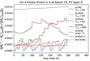
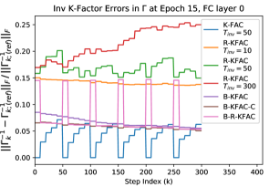
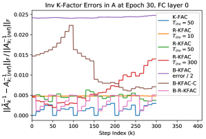
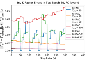
Figure 1: Error in inverse K-Factors. Each curve is the average over 5 runs.

4.3 Numerical Error Investigation: Results

Figure 1 shows the error metrics (1) and (2). Figure 2 shows the error metrics (3) and (4). Error metric and epoch vary across columns and rows respectively.

Error Periodicity and “Reset Times”. Note that aside from b-kfac and r-kfac with $T_{\text{inv}}=300$, all other algorithms have a period of 50 steps. This arises because these algorithms have a heavier update every $50$ step (either an rsvd-overwriting of “$\mathcal{B}_{k}$”, or a correction), and a lighter (or no) update every 10 steps. The numerical results show that performing an over-writing of “$\mathcal{B}_{k}$” (see b-r-kfac) or an EVD recomputation of inverse K-factor (see k-fac $T_{\text{inv}}=50$) always resets the error back to roughly the same level, while performing a correction reduces the error down to more variable levels (see b-kfac-c). This is intuitive: unlike the other two heavy updates, the correction’s output depends on the approximate K-factor inverse representation to be corrected.

R-KFAC $T_{\text{inv}}=50$ vs K-FAC $T_{\text{inv}}=50$. We see that the error patterns of these two algorithms are very similar. The error of r-kfac is only mildly larger than the one of k-fac, showing there is significant eigenspectrum decay ([3]).

B-R-KFAC vs R-KFAC: Relationship to Propositions 4.1 and 4.2. There are two important comparisons to note here. First, comparing b-r-kfac and r-kfac with $T_{inv}=50$, we see that performing a b-update is almost always better than performing no update in terms of all error metrics and for all considered epochs (at least for the considered set-up). This result for the first two error metrics relates strongly to Proposition 4.2, but further to the weaker result that the theory predicts, it shows that the error in K-Factors is almost always better when a b-update is performed than when no update is performed.

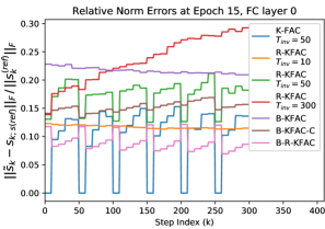
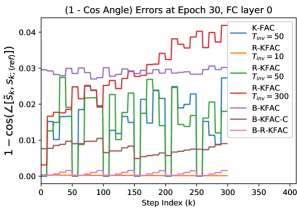
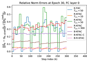
Figure 2: Error in Step. Since the gradient changes at each location, the error in step typically changes on every iteration, even though the error in K-Factor can change only once every 10 iterations. Thus, we effectively have 10 different samples from the distribution of step-error for each given $\{\text{approximate K-Factor representation, Benchmark K-Factor}\}$ pair. We report the average over these 10 samples only (giving us a constant error over iterations 200-209 for instance). As before, we further average over 5 runs.

Secondly, comparing the results of b-kfac and r-kfac $T_{\text{inv}}=300$ is effectively comparing the steady-state error of b-kfac with the error of "no reset" r-kfac (which performs one r-kfac update at the beginning of the examined period, and no updates thereafter). We see that for all error metrics, the error of b-kfac is fairly constant while the error of r-kfac $T_{\text{inv}}=300$ grows fast. The error of the latter algorithm very rapidly exceeds the one of b-kfac for the second error metric. In relation to Proposition 4.1, this suggests that $\left\lVert E_{j}\right\rVert_{F}$ is much larger for no-update than for b-updates when $\mathcal{M}_{k}=\bar{\Gamma}_{k}$. While the same phenomenon did not occur on the 300 steps interval considered for error metric (1) and K-factor $\bar{\mathcal{A}}_{k}$, this would have occurred about 900 steps later.

From a more practical point of view, the step-related error metrics (in Figure 2) of “no reset” r-kfac rapidly increase past the steady-state error of b-kfac, despite the behaviour in error metric (1). Thus, the errors we are most interested in are much more favorable when using b-updates than when using no updates. For example, at epoch 15, it took only 10-15 skipped inverse-updates after an r-kfac update for the step-error to exceed the steady-state level of b-kfac.

B-KFAC vs B-R-KFAC: Relationship to Proposition 3.2. Figures 1 and 2 show that when adding periodic rsvd overwritings to a b-kfac algorithm, the error is better for all iterations (compare plots of b-kfac with plots of b-r-kfac). This aligns with the intuition we have developed from Proposition 3.2.

B-KFAC vs B-R-KFAC vs B-KFAC-C. The error of b-kfac-c lies in between the one of (the more expensive) b-r-kfac and (the cheaper) b-kfac. Thus, b-kfac-c allows us to trade between CPU time and error by tuning $\phi_{corct}$.

Average Error in Relation to Time-per-Epoch ($t_{\text{epoch}}$). It is instructive to consider the relationship between average error and $t_{\text{epoch}}$. Table 1 summarizes the results in Figures 1 and 2, but also shows $t_{\text{epoch}}$ measurements. The average-error order obviously carries on from the one observable in Figures 1 and 2, while the $t_{\text{epoch}}$ ordering is what one would expect based on our discussions in Section 3. Note that when considering $t_{\text{epoch}}$, the fair comparison between b-kfac and r-kfac is when the latter has $T_{\text{inv}}=10$ (both perform an inverse-update every 10 steps). In this case, we see that b-kfac is much cheaper than r-kfac. However, increasing $T_{\text{inv}}$ to $T_{\text{inv}}=50$ gets r-kfac slightly cheaper per epoch than b-kfac.

No algorithm has all metrics better than any other. Thus, we cannot say which one will give better optimization performance. However, we can see that r-kfac has significantly smaller $t_{\text{epoch}}$ than k-fac with only marginally larger error, suggesting r-kfac will most likely perform better in practice (reconciling with findings in [3]). We can also see we dramatically reduce error of r-kfac ($T_{\text{inv}}=50$) by adding in b-updates (getting b-r-kfac), while the $t_{\text{epoch}}$ overhead is minimal (reconciles with our discussion in Section 3). Finally, we see some of b-r-kfac’s accuracy can be given away in exchange for slightly smaller $t_{\text{epoch}}$ by turning the rsvd-overwriting either into a correction (getting b-kfac-c), or into a b-update (getting b-kfac). Note that changes in $t_{\text{epoch}}$ are relatively small when taking out/putting in b-updates, because these updates are applied only to the first FC layer, but $t_{\text{epoch}}$ measures computations across all the layers.

Table 1: Avg. Error Metrics (of each error curve at epoch 30) and $t_{\text{epoch}}$ (mean $\pm$ SD).

Optimizer	Avg. Err. metric 1	Avg. Err. metric 2	Avg. Err. metric 3	Avg. Err. metric 4	$t_{\text{epoch}}$ (s)
k-fac $T_{\text{inv}}=50$	1.51e-03	8.42e-02	2.69e-01	14.4e-02	$169\pm 5.6$
r-kfac $T_{\text{inv}}=50$	4.65e-03	10.4e-02	2.96e-01	14.6e-02	$58.5\pm 0.6$
r-kfac $T_{\text{inv}}=10$	4.8e-03	4.9e-02	0.43e-01	0.02e-02	$71.2\pm 1.0$
b-kfac	48.6e-03	1.02e-02	2.40e-01	29.0e-02	$59.2\pm 0.6$
b-kfac-c	11.9e-03	1.04e-02	1.22e-01	0.77e-02	$59.4\pm 0.6$
b-r-kfac	3.40e-03	1.81e-02	0.40e-01	0.74e-02	$59.5\pm 0.6$

5 Proposing a K-factor Inverse Application which is Linear in $d_{M}$

So far, we have seen that for certain layers we can use the B-update to obtain low-rank inverse representations of K-factors in linear time in $d_{M}$ (though with no error guarantee). To reap the most benefits, we would like the inverse application itself to also scale no worse than linear in $d_{M}$. With the inverse application procedure proposed in Algorithm 1, we saw we could make it quadratic. In this section, we argue that, for the layers where applying the B-update makes sense, we can make our inverse application linear in $d_{M}$ as well.

However, in our numerical experiments we did not implement this feature, and left this as future work!

The idea behind our approach is simple: the gradient of each layer (in matrix form, $\text{Mat}(g^{(l)})$) is a of the form (at iteration $k$)

$$\text{Mat}(g_{k}^{(l)})=G^{(l)}_{k}[A_{k}^{(l)}]^{T},$$ (20)

where $G^{(l)}_{k}\in\mathbb{R}^{d_{\Gamma}^{(l)}\times n_{M}^{(l)}}$ and $G^{(l)}_{k}\in\mathbb{R}^{d_{\mathcal{A}}^{(l)}\times n_{M}^{(l)}}$ are the same matrices as the ones used to generate the EA K-factors as (review Section 1.5).

Thus, we see that whenever the B-update is applicable ($n_{M}^{(l)}<n_{BS}+d_{\mathcal{A}}^{(l)}$ for the “A” K-factors, and $n_{M}^{(l)}<n_{BS}+d_{\Gamma}^{(l)}$ for the “G” K-factors), we can make further computational savings by avoiding the multiplication of $G^{(l)}_{k}[A_{k}^{(l)}]^{T}$ in the backward pass and applying the inverse representation by first taking a product with $G^{(l)}_{k}$, and then with $A_{k}^{(l)}$. That is, we compute the product $[\bar{\Gamma}^{(l)}]^{-1}\text{Mat}(g_{k}^{(l)})[\bar{\mathcal{A}}^{(l)}_{k}]^{-1}$ as

$$[\bar{\Gamma}^{(l)}_{k}]^{-1}\text{Mat}(g_{k}^{(l)})[\bar{\mathcal{A}}^{(l)}_{k}]^{-1}=\biggl{(}[\bar{\Gamma}_{k}^{(l)}]^{-1}G^{(l)}_{k}\biggr{)}\biggl{(}[A_{k}^{(l)}]^{T}[\bar{\mathcal{A}}^{(l)}_{k}]^{-1}\biggr{)},$$ (21)

but of course we use our low-rank inverse representations for $[\bar{\Gamma}_{k}^{(l)}]^{-1}$ and $[\bar{\mathcal{A}}^{(l)}_{k}]^{-1}$ rather than the standard EVD inverses. Algorithm 8 shows how this works in practice.

1 // The low-rank inverse representation of $[\bar{\Gamma}^{(l)}]^{-1}$ and $[\bar{\mathcal{A}}^{(l)}_{k}]^{-1}$ are required

2

3Modify the back-prop to return $G^{(l)}_{k}$, $A_{k}^{(l)}$ rather than $\text{Mat}(g_{k}^{(l)})$

4Replace the lines 8-10 of Algorithm 1 with: // Apply the low-rank inverse representation with linear time in $d_{\Gamma}$ and $d_{\mathcal{A}}$

5

6 // Estimate $[A_{k}^{(l)}]^{T}[\bar{\mathcal{A}}^{(l)}_{k}]^{-1}$, use the lowrank represent. of $\bar{\mathcal{A}}^{(l)}_{k}$:

7 $[\mathbf{A}^{(l)}_{k}]^{T}:=[A^{(l)}_{k}]^{T}\tilde{V}^{(l)}_{A,k}\big{[}(\tilde{D}^{(l)}_{A,k}+\lambda I)^{-1}-\frac{1}{\lambda}I\big{]}(\tilde{V}^{(l)}_{A,k})^{T}+\frac{1}{\lambda}[A^{(l)}_{k}]^{T}$ ;

8  // $\mathcal{O}(rd_{\mathcal{A}}^{(l)}n_{M}^{(l)})$

9

10 // Estimate $[\bar{\Gamma}^{(l)}_{k}]^{-1}G^{(l)}_{k}$, use the lowrank represent. of $\bar{\Gamma}^{(l)}$:

11 $\mathbf{G}_{k}^{(l)}:=\tilde{V}^{(l)}_{\Gamma,k}\biggl{[}(\tilde{D}^{(l)}_{\Gamma,k}+\lambda I)^{-1}-\frac{1}{\lambda}I\biggr{]}(\tilde{V}^{(l)}_{\Gamma,k})^{T}G^{(l)}_{k}+\frac{1}{\lambda}G^{(l)}_{k}$ ;

12  // $\mathcal{O}(rd_{\Gamma}^{(l)}n_{M}^{(l)})$

13

// Construct the Precond. Step from Partial Quantities:

15 $S^{(l)}_{k}=\mathbf{G}_{k}^{(l)}[\mathbf{A}^{(l)}_{k}]^{T}$ // $S^{(l)}_{k}$ is the step for layer $l$ in matrix form

16

Algorithm 8 Linear Inverse Application: works whenever (b-update) can be applied

We thus see that whenever the B-update is applicable ($n_{M}^{(l)}<n_{BS}+d_{\mathcal{A}}^{(l)}$ for the “A” K-factors, and $n_{M}^{(l)}<n_{BS}+d_{\Gamma}^{(l)}$ for the “G” K-factors), we reduce the time scaling of our inverse application from $\mathcal{O}(r([d_{\Gamma}^{(l)}]^{2}+[d_{\mathcal{A}}^{(l)}]^{2}))$ (as we had in R-KFAC, Algorithm 1), to $\mathcal{O}(r(d_{\Gamma}^{(l)}+d_{\mathcal{A}}^{(l)})n_{M}^{(l)})$. This inverse application methodology offers:

1. An improved inverse application complexity down to linear in layer size for all K-factors;

2. A concrete, practical computational saving whenever the B-update is applicable (since $n_{M}<d_{M}$ when this happens).

6 Numerical Results

6.0.1 Implementation details

We now compare the numerical performance of our proposed algorithms: b-kfac, b-r-kfac or b-kfac-c, with relevant benchmark algorithms: r-kfac (Algorithm 1; [3]), k-fac ([1]), and seng (the state of art implementation of NG for DNNs; [5]). We consider the CIFAR10 classification problem with a modified version of batch-normalized VGG16 (VGG16_bn). All experiments ran on a single NVIDIA Tesla V100-SXM2-16GB GPU. The accuracy and loss we refer to are always on the test set.

For seng, we used the official github repo implementation with the hyperparameters directly recommended by the authors for the problem at hand.

For all algorithms except seng, we use $\rho=0.95$, $n_{\text{BS}}=256$ and $T_{\text{updt}}=25$, weight decay of $7e-04$, no momentum, a clip parameter of $0.07$ and a learning rate schedule of $\alpha_{k}=0.3-0.1\mathbb{I}_{n_{ce}(k)\geq 2}-0.1\mathbb{I}_{n_{ce}(k)\geq 3}-0.07\mathbb{I}_{n_{ce}(k)\geq 13}-0.02\mathbb{I}_{n_{ce}(k)\geq 18}-0.007\mathbb{I}_{n_{ce}(k)\geq 27}-0.002\mathbb{I}_{n_{ce}(k)\geq 40}$ (where $n_{\text{ce}}(k)$ is the number of the current epoch at iteration $k$). For all these algorithms, we set the regularization to be depend on layer, K-factor type ($\mathcal{A}$ vs $\Gamma$), and iteration as $\lambda_{k,l}^{(\mathcal{M})}=\lambda_{\text{max},k,l}^{(\mathcal{M})}\phi_{\lambda,k}$ with the schedule $\phi_{\lambda,k}=0.1-0.05\mathbb{I}_{n_{\text{ce}}(k)\geq 25}-0.04\mathbb{I}_{n_{\text{ce}}(k)\geq 35}$.

For k-fac and r-kfac we set $T_{\text{inv}}=250$. We also consider an r-kfac which uses all the previous settings but $T_{\text{inv}}=25$ - we refer to it “r-kfac $T_{\text{inv}}=25$”. The hyperparameters specific to r-kfac were set to $n_{\text{pwr-it}}=4$, target-rank schedule $r(k)=220+10\mathbb{I}_{n_{\text{ce}(k)}\geq 15}$, and oversampling parameter schedule $r_{o}(k)=10+\mathbb{I}_{n_{ce}(k)\geq 22}+\mathbb{I}_{n_{\text{ce}(k)}\geq 30}$ (see [3] for details).

For b-kfac, b-r-kfac and b-kfac-c we set the truncation rank schedule to be the same as the target-rank schedule ($r(k)$) of r-kfac. For b-kfac we used $T_{\text{Brand}}=125$. b-kfac-c had $T_{\text{Brand}}=125$, $T_{corct}=500$, and $\phi_{corct}=0.5$. b-r-kfac had $T_{\text{Brand}}=25$, and $T_{\text{RSVD}}=250$.

Recall from Section 3.5 that the implemented b-kfac, b-r-kfac and b-kfac-c use the corresponding proposed updates only for the first FC layer, and r-kfac updates (Algorithm 1; [3]) for all other layers. The hyperparameters of the r-kfac part of b-kfac, b-r-kfac or b-kfac-c are the ones we described above.

6.1 Algorithms Optimization Performance Comparison

Table 2 shows a summary of results. We make the following observations:

Benchmark 0: seng. Relatively large number of epochs to target accuracy but very low $t_{\text{epoch}}$, giving the best performance across all benchmarks (and all algorithms in general) for all target test accuracies apart from $91\%$.

Benchmark 1: k-fac. the weakest of all algorithms with very large $t_{\text{epoch}}$, and surprisingly (unknown reason), much larger no. of epochs to target accuracy than any of its sped-up versions (all of which approximate the K-factors).

Benchmark 2: r-kfac. Moderate number of epochs to certain accuracy and moderate $t_{\text{epoch}}$, giving a performance always better than k-fac (benchmark 1). Nevertheless, it only outperforms seng (benchmark 0) for $91\%$ test accuracy.

b-kfac: Has the lowest computational cost per epoch ($t_{\text{epoch}}$) across all kfac-based algorithms, while taking nearly the same amount of epochs to a target test accuracy as the other kfac-based algorithms. It outperforms k-fac and r-kfac (benchmarks 1 and 2) for all considered target accuracies, being the best performing b-$(\cdot)$ variant. It outperforms seng only for $91\%$ test accuracy.

b-r-kfac: essentially upgrades r-kfac (with $T_{inv}=250$) to also perform a b-update every time new K-factor information arrives. This improves $\mathcal{N}_{\text{acc}\geq 93\%}$ but makes $t_{\text{epoch}}$ worse. Over-all it seems that the extra accuracy gained through introducing b-updates is favourable for large target test accuracy: b-r-kfac reaches $93.5\%$ acc. 8 times while r-kfac ($T_{\text{inv}}=250$ never does so).

b-kfac-c: Lies in between b-kfac and b-r-kfac in terms of both $t_{\text{epoch}}$ and $\mathcal{N}_{\text{acc}\geq 93\%}$, but provids a worse cost-accuracy trade-off than either of these in this case. Nevertheless, it outperforms r-kfac and k-fac benchmarks for all considered target test accuracies, and outperforms seng for low target accuracy.

Table 2: Optimizer Performance Results Summary. We perform 10 runs of 50 epochs for each considered solver. Columns 2-4 show times to a target test accuracy. Columns 5 shows the time per epoch. Column 6 shows how many runs get to $93.5\%$ test accuracy. All solvers get to $93\%$ accuracy 10 out of 10 times. The final column shows the number of epochs to $93\%$ test accuracy. All results concerning times and number of epochs are shown as empirical mean $\pm$ empirical st. dev. The results for columns 2,3,7 use 10 samples (since 10/10 runs get to $93\%$ acc.). The results in column 5 use only the runs which got to $93.5\%$. The results in column 5 use $500$ samples. All times are in seconds.

	$t_{acc\geq 91\%}$	$t_{acc\geq 93\%}$	$t_{acc\geq 93.5\%}$	$t_{\text{epoch}}$	$\#$ hit $93.5\%$	$\mathcal{N}_{\text{acc}\geq 93\%}$
seng	$999.0\pm 54.1$	$1098,\pm 37.5$	$1144\pm 51$	$25.4\pm 0.81$	10 in 10	$43.1\pm 1.5$
k-fac	$2610\pm 213$	$4021\pm 433$	N/A	$97.8\pm 8.2$	0 in 10	$41.1\pm 4.6$
r-kfac	$920.3\pm 24.5$	$1357\pm 38.7$	N/A	$47.7\pm 0.54$	0 in 10	$28.9\pm 0.8$
r-kfac $T_{\text{inv}}=25$	$1019\pm 3.05$	$1526\pm 49.3$	$2108\pm 373$	$53.3\pm 0.69$	6 in 10	$28.5\pm 0.9$
b-kfac	$894.0\pm 22.9$	$1325\pm 58.9$	$1913\pm 125$	$46.3\pm 0.62$	10 in 10	$28.6\pm 1.2$
b-kfac-c	$911.2\pm 18.9$	$1352.3\pm 32.54$	$2031\pm 312$	$47.4\pm 0.45$	6 in 10	$28.5\pm 0.7$
b-r-kfac	$945.9\pm 39.6$	$1324.8\pm 58.9$	$1975\pm 323$	$48.4\pm 0.53$	8 in 10	$28.3\pm 0.5$

7 Conclusion

By exploiting the EA construction paradigm of the K-factors, we proposed an online inverse-update to speed-up k-fac ([1]) for FC layers. If we use the update exclusively, we obtian the K-factor inverse representation in linear time scaling w.r.t. layer size (as opposed to quadratic for r-kfacs [3], and cubic for standard k-fac [1], [2]). This update relied on Brand’s algorithm ([4]), and we called it the “b-update” (of K-factors inverses). We saw the update is useful only when $d_{M}>n_{M}+r$, which typically holds for FC layers.

In these cases, we saw the b-update is exact, but only remains cheap if we constrain our approximate K-Factors representation to be (very) low-rank - which we practically achieved through an SVD-optimal rank-$r$ truncation just before each b-update. We argued that based on results presented in [3], (EA) K-Factors typically have significant eigenspectrum decay, and thus a very low-rank approximation for them would actually have low error.

We also saw that whenever we can apply the B-update, our inverse application technique can be improved to reduce time scaling from quadratic in layer size (as for rs-kfac) down to linear. We did not implement this inverse application methodology in this paper however (this is future work).

The b-update, together with the truncation, and the proposed inverse application technique gave b-kfac. The algorithm (b-kfac) is an approximate k-fac implementation for which the preconditioning part scales (over-all) linearly in layer size. Notably however, “pure” b-kfac is only applicable to some layers (and we have to use rs-kfac for the others). Compared to quadratic scaling in layer size for rs-kfac ([8]) or cubic for k-fac ([1], [2]), the improvement proposed here is a substantial improvement. Though there is no error guarantee bounding the b-kfac preconditioning error, we saw with numerical case-studies which revealed the b-kfac error was acceptable.

We saw that the b-update, other than being used alone to give b-kfac, can also be combined with updates like rs-kfac updates (rsvd updates) to give different algorithms with different empirical properties. By comparing b-kfac with r-kfac (rs-kfac in [3]), we noted that we may be able to increase the K-Factor representation accuracy of b-kfac by adding in periodic rsvd “overwritings”, which gave the b-r-kfac algorithm. We saw that the b-r-kfac can also be seen as an r-kfac algorithm to which we introduce b-updates at times when no rsvd would have been performed, with the aim of better controlling the K-factor representation error, at minimal cost. We also noted we may change the rsvd-overwriting with a cheaper but less accurate “correction”, in order to obtain customizable time-accuracy trade-offs, giving b-kfac-c.

Numerical results concerning K-Factors errors show that our all our proposed algorithms (b-kfac, b-r-kfac, and b-kfac-c) had errors comparable to k-fac ([1]) while offering an $\approx 3\times$ speed-up per epoch. W.r.t. the more competitive r-kfac ([3]), our proposed algorithms offered similar metrics but more trade-offs to choose from. Notably, b-r-kfac was significantly better than r-kfac - across all investigated error metrics at minimal computational overhead. Numerical results concerning optimization performance show b-kfac and b-kfac-c consistently outperform r-kfac (the best k-fac benchmark; [3]) by a moderate amount, while b-r-kfac only does so for relatively large target test accuracy. All our b-$(\cdot)$ algorithms outperform seng (the state of art; [5]) for low target test accuracy.

Future work involves implementing the proposed inverse application methodology and re-running numerical experiments.

7.0.1 Acknowledgments

Thanks to Jaroslav Fowkes and Yuji Nakatsukasa for useful discussions. I am funded by the EPSRC CDT in InFoMM (EP/L015803/1) together with Numerical Algorithms Group and St. Anne’s College (Oxford).

References

• [1] Martens, J.; Grosse, R. Optimizing neural networks with Kronecker-factored approximate curvature, In: arXiv:1503.05671 (2015).
• [2] Grosse, R.; Martens J. A Kronecker-factored approximate Fisher matrix for convolution layers, arXiv:1602.01407 (2016).
• [3] Puiu, C. O. Randomized KFACs: Speeding up K-FAC with Randomized Numerical Linear Algebra, arXiv:2206.15397 (2022).
• [4] Brand, M. Fast Low-Rank Modifications of the Thin Singular Value Decomposition, Linear Algebra and its Applications Volume 415, Issue 1, pp. 20-30, 2006.
• [5] Yang, M.; Xu, D; Wen, Z.; Chen, M.; Xu, P. Sketchy empirical natural gradient methods for deep learning, arXiv:2006.05924 (2021).
• [6] Martens, J. New insights and perspectives on the natural gradient method, arXiv:1412.1193 (2020).
• [7] Amari, S. I. Natural gradient works efficiently in learning, Neural Computation, 10(20), pp. 251-276 (1998).
• [8] Halko N.; Martinsson P.G.; Tropp J. A. Finding structure with randomness: Probabilistic algorithms for constructing approximate matrix decompositions, SIAM Review, 53(2), pp. 217-288 (2011).
• [9] Tang, Z.; Jiang, F.; Gong, M.; Li, H.; Wu, Y.; Yu, F.; Wang, Z.; Wang, M. SKFAC: Training Neural Networks with Faster Kronecker-Factored Approximate Curvature, IEEE/CVF Conference on Computer Vision and Pattern Recognition, (2021).
• [10] Osawa, K.; Yuichiro Ueno, T.; Naruse, A.; Foo, C.-S.; Yokota, R. Scalable and practical natural gradient for large-scale deep learning, arXiv:2002.06015 (2020).
• [11] Saibaba, A. K. Randomized subspace iteration: Analysis of canonical angles and unitarily invariant norms, arXiv:1804.02614 (2018).
• [12] Mazeika M. The Singular Value Decomposition and Low Rank Approximation.