Scratching Visual Transformer’s Back
with Uniform Attention

Abstract

The favorable performance of Vision Transformers (ViTs) is often attributed to the multi-head self-attention ($\mathtt{MSA}$). The $\mathtt{MSA}$ enables global interactions at each layer of a ViT model, which is a contrasting feature against Convolutional Neural Networks (CNNs) that gradually increase the range of interaction across multiple layers. We study the role of the density of the attention. Our preliminary analyses suggest that the spatial interactions of attention maps are close to dense interactions rather than sparse ones. This is a curious phenomenon, as dense attention maps are harder for the model to learn due to steeper softmax gradients around them. We interpret this as a strong preference for ViT models to include dense interaction. We thus manually insert the uniform attention to each layer of ViT models to supply the much needed dense interactions. We call this method Context Broadcasting, $\mathtt{CB}$. We observe that the inclusion of $\mathtt{CB}$ reduces the degree of density in the original attention maps and increases both the capacity and generalizability of the ViT models. $\mathtt{CB}$ incurs negligible costs: 1 line in your model code, no additional parameters, and minimal extra operations.

1 Introduction

After the success of Transformers (Vaswani et al., 2017) in language domains, Dosovitskiy et al. (2021) have extended to Vision Transformers (ViTs) that operate almost identically to the Transformers but for computer vision tasks. Recent studies (Dosovitskiy et al., 2021; Touvron et al., 2021b) have shown that ViTs achieve superior performance on image classification tasks.

The favorable performance is often attributed to the multi-head self-attention ($\mathtt{MSA}$) in ViTs (Dosovitskiy et al., 2021; Touvron et al., 2021b; Wang et al., 2018; Carion et al., 2020; Strudel et al., 2021; Raghu et al., 2021), which facilitates long-range dependency. Specifically, $\mathtt{MSA}$ is designed for global interactions of spatial information in all layers. This is a structurally contrasting feature with a large body of successful predecessors, convolutional neural networks (CNNs), which gradually increase the range of interactions by stacking many fixed and hard-coded local operations, i.e., convolutional layers. Raghu et al. (2021) and Naseer et al. (2021) have shown the effectiveness of the self-attention in ViTs for the global interactions of spatial information compared to CNNs.

Unlike previous work that focused on the effectiveness of long-range dependency, we study the role of density of spatial attention. Long-range dependency, or global interactions, signifies connections that reach distant locations from the reference token. Density refers to the proportion of non-zero interactions across all tokens. We illustrate the difference between the two in Fig. 1. Observe that “global” does not necessarily mean “dense” and vice versa because an attention map can be either densely local or sparsely global.

We first examine whether a ViT model learns dense or sparse attention maps. Our preliminary analysis based on the entropy measure suggests that the learned attention maps tend to be dense across all spatial locations. This is a curious phenomenon because denser attention maps are harder to learn. Self-attention maps are the results of softmax operations. As we show in our analysis, the gradients become less stable around denser attention maps. In other words, ViTs are trying hard to learn dense attention maps despite the difficulty of learning them through gradient descent.

While it is difficult to learn dense attention via gradient descent, it is easy to implement it manually. We insert uniform attention, the densest form of attention, via average pooling across all tokens. We call our module Context Broadcasting ($\mathtt{CB}$). The module adds the average-pooled token to every individual token at each intermediate layer.

We find that when $\mathtt{CB}$ is added to a ViT model, it reduces the degree of density in attention maps in all layers. $\mathtt{CB}$ also makes the overall optimization for a ViT model easier and improves its generalization. $\mathtt{CB}$ module brings consistent gains in the image classification task on ImageNet (Russakovsky et al., 2015; Recht et al., 2019; Beyer et al., 2020) and the semantic segmentation task on ADE20K (Zhou et al., 2017; 2019). Overall, $\mathtt{CB}$ module seems to help a ViT model divert its resources from learning dense attention maps to learning other informative signals.

Such benefits come with only negligible costs. Only 1 line of code needs to be inserted in your model.py. No additional parameters are introduced; only a negligible number of operations are.

Our contributions are:

• Our observations that ViTs benefit from further dense interactions (Sec. 2.1);

• A simple and effective modules, $\mathtt{CB}$ and $\mathtt{CB_{S}}$, for infusing dense interactions (Sec. 2.2);

• Experimental results verifying the benefits of $\mathtt{CB}$ and $\mathtt{CB_{S}}$ (Sec. 3).

2 Method

We first motivate the need for further dense interactions for the ViT architectures in Sec. 2.1. Then, we propose a simple, lightweight module and a technique to explicitly inject dense interactions into ViTs in Sec. 2.2.

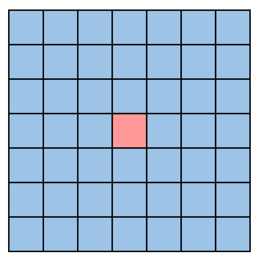
(a) Dense global

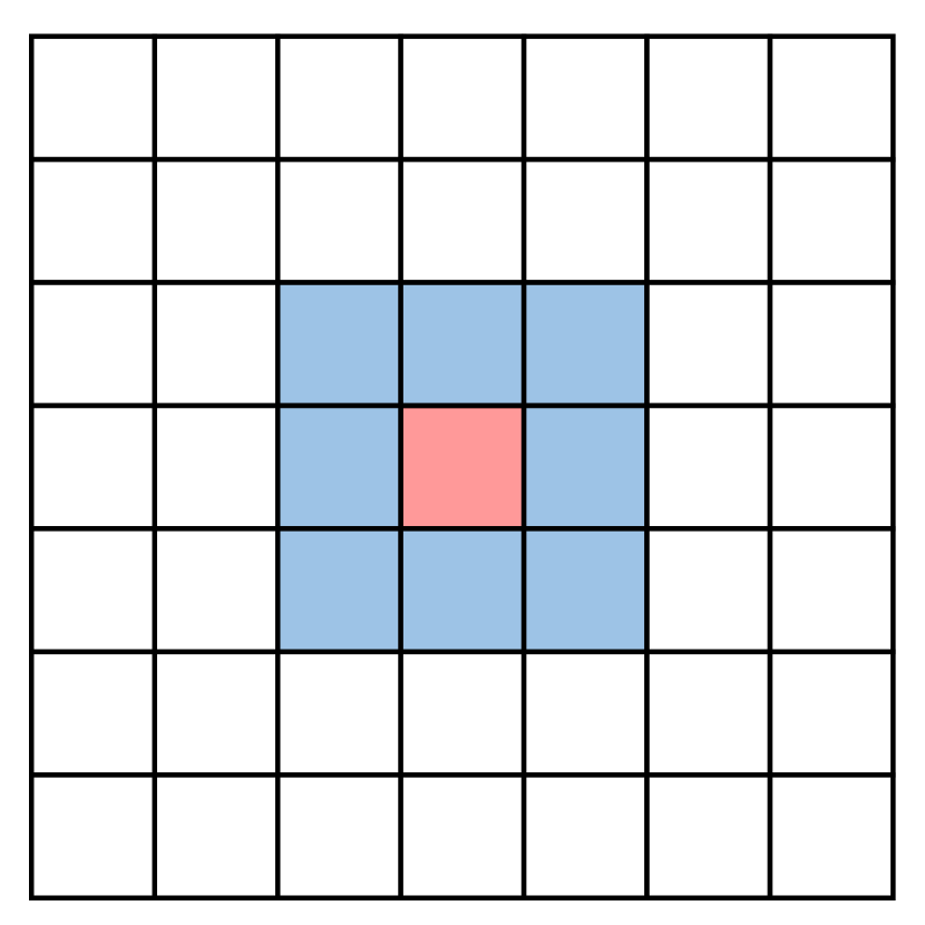
(b) Dense local

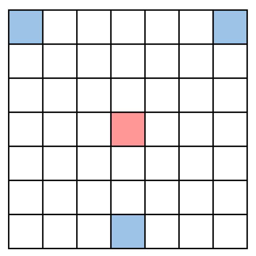
(c) Sparse global

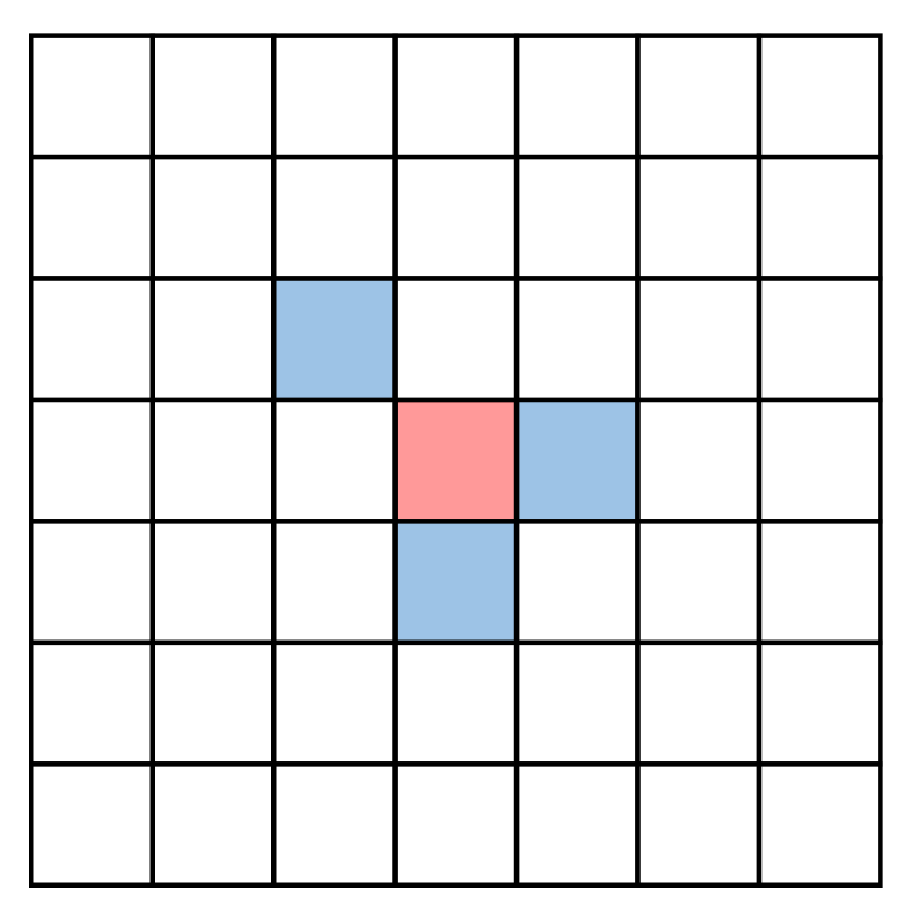
(d) Sparse local

Figure 1: Type of spatial interactions. We categorize the spatial interactions into a combination of {Dense, Sparse} and {Global, Local}. The anchor token interacts with reference tokens.

2.1 Motivation

The self-attention operations let ViTs conduct spatial interactions without limiting the spatial range in every layer. Despite the inherent abundance of such operations compared to CNNs, we study the density of the attention. The first experiment examines whether ViTs need further spatial interactions. In the second experiment, we measure the layer-wise entropy of the attention to examine what characteristics of spatial interactions ViTs prefer to learn.

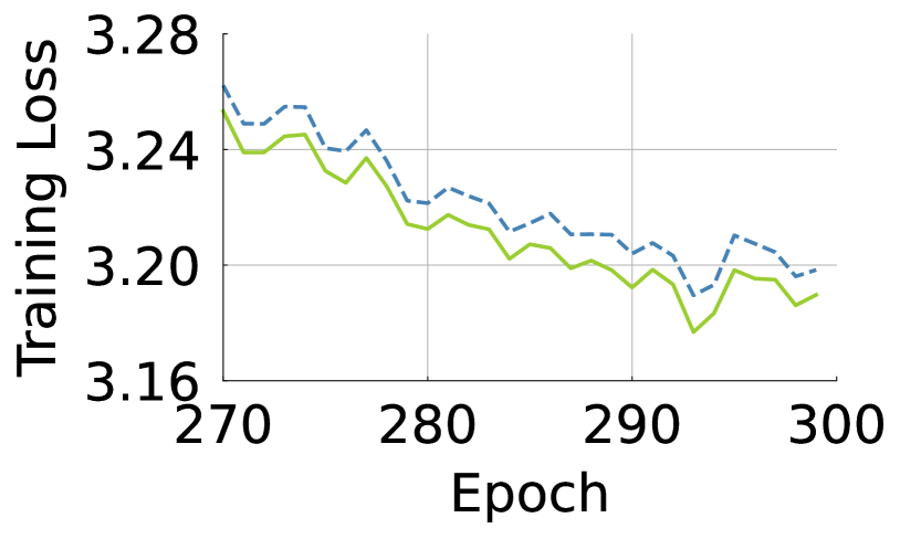
(a) Training Loss

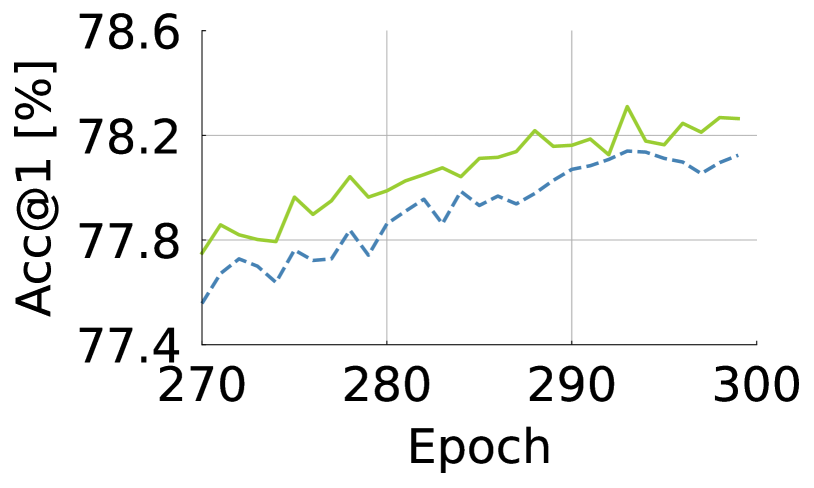
(b) Top-1 Accuracy

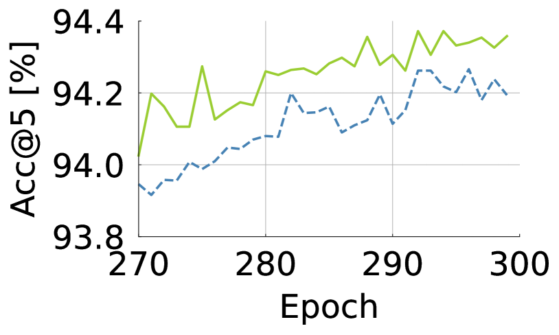
(c) Top-5 Accuracy

Figure 2: Impact on the capacity of the ViT model with a single extra block. Training loss, top-1 accuracy, and top-5 accuracy ($y$-axis) versus epochs ($x$-axis) of 8-depth ViT with additional $\mathtt{MSA}$ and $\mathtt{MLP}$ blocks. The decrease in training loss and the increase in validation accuracies imply an increase in the model capacity.

Are ViTs hungry for more spatial connections?

The multi-head self-attention ($\mathtt{MSA}$) and multi-layer perceptron ($\mathtt{MLP}$) in ViTs are responsible for spatial and channel interactions, respectively. We examine adding which block, either $\mathtt{MSA}$ or $\mathtt{MLP}$, increases the performance of ViTs more. We train the eight-layer ViT on ImageNet-1K for 300 epochs with either an additional $\mathtt{MSA}$ or $\mathtt{MLP}$ layer inserted at the last layer. The additional number of parameters and FLOPs are nearly equal. In Fig. 2, we plot the training loss and top-1/5 accuracies. We observe that the additional $\mathtt{MSA}$ enables lower training loss and higher validation accuracies than the additional $\mathtt{MLP}$. This suggests that, given a fixed budget in additional parameters and FLOPs, ViT architectures seem to prefer to have extra spatial interactions rather than channel-wise interactions.

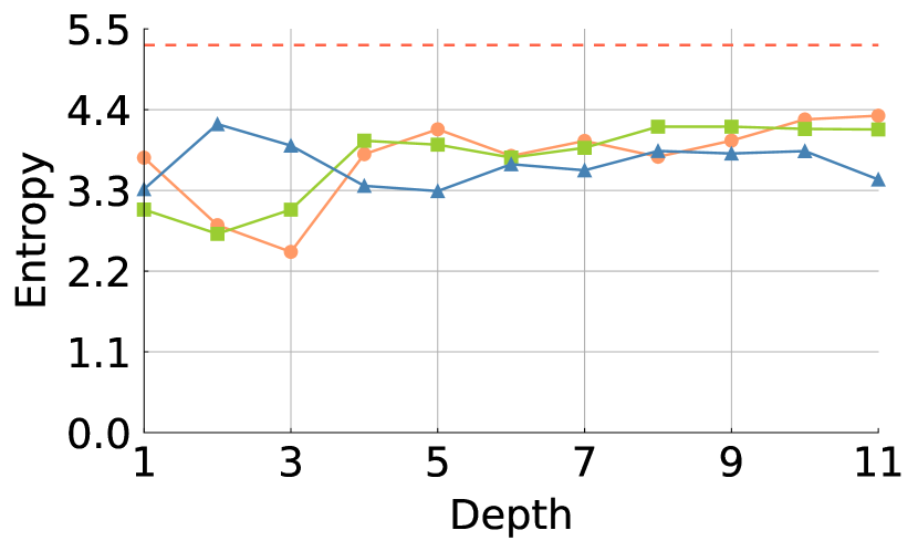
(a) Entropy of attention

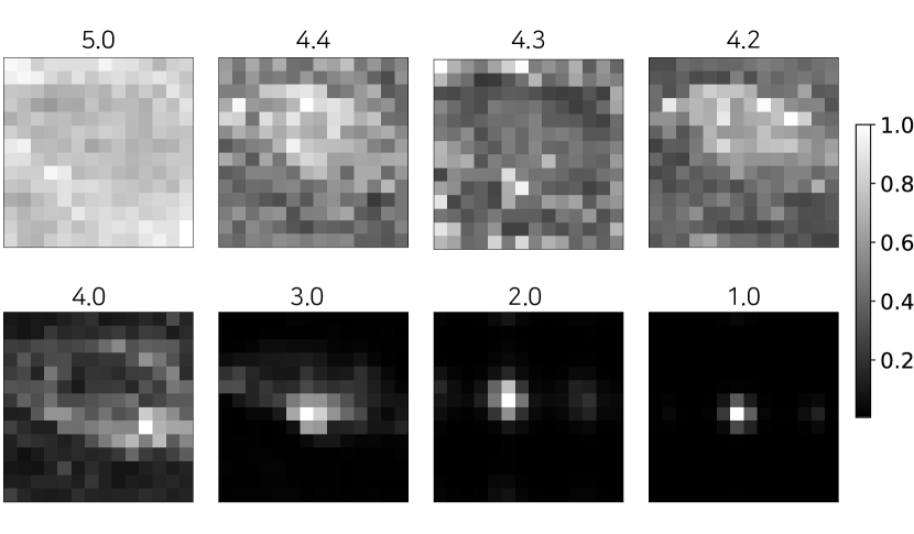
(b) Visualization of entropy

Figure 3: Entropy analysis and visualization. (a) We use the ImageNet-1K trained ViT-Ti/-S/-B and exclude the last layers and the class token in computing the values. The red dot line means the maximum entropy upper bound. (b) For reference and an intuitive interpretation of entropy values, we visualize samples of attention maps for an image from low to high entropy values using ViT-S. We denote the value of entropy above visualizations.

Which type of spatial interactions do $\mathtt{MSA}$ learn?

In this experiment, we examine the types of spatial interactions that are particularly preferred by $\mathtt{MSA}$. Knowing the type of interactions will guide us on how we could improve attention performance. While previous studies have focused on the effectiveness of long-range dependency in $\mathtt{MSA}$, we focus on the density in $\mathtt{MSA}$. We measure the dispersion of attention according to the depth through the lens of entropy. When the attention is sparse, the entropy of attention is low. On the flip side, when the attention is dense, the entropy of it is high. Figure 3(a) shows the trends of the average entropy values across the heads and tokens for each $\mathtt{MSA}$ layer in ViT-Ti/-S/-B (Dosovitskiy et al., 2021; Touvron et al., 2021b). We observe that attention maps tend to have greater entropy values as high as 4.4, towards the maximal entropy value, $-\sum\tfrac{1}{N}\log\tfrac{1}{N}\approx 5.3$, for attention maps given $N=197$. To provide an intuitive interpretation of entropy value, we visualize the attention maps of a training sample from the pre-trained ViT-S. We also visualize the attention with low entropy values just for comparison purpose. Figure 3(b) depicts the extent of attention map density according to entropy values, where densely distributed weights are observed in the attention maps having entropy values as high as the observed average entropy, 4.4. It is quite remarkable that a majority of the attention in ViTs have such high entropy values; it suggests that $\mathtt{MSA}$ tends to learn the dense interactions.

Steepest gradient around the uniform attention.

The extreme form of dense interactions is the uniform distribution. To examine the difficulty of finding the uniform distribution solution for the attention mechanism, we delve into the characteristics of the $\mathtt{softmax}$ function. In a nutshell, we show that the gradient magnitude is the greatest around the inputs inducing a uniform output. We further formalize this intuition below. The attention mechanism consists of the row-wise softmax operation $\mathbf{A}=\sigma(\lambda\mathbf{S})\in\mathbb{R}^{N\times N}$ where $\mathbf{S}\in\mathbb{R}^{N\times N}$ is the collection of dot products of queries and keys, possibly with a scale factor $\lambda>0$. For simplicity, we consider the softmax over a single row: ${\mathbf{a}}=\sigma(\lambda{\mathbf{s}})\in\mathbb{R}^{N}$. The gradient of ${\mathbf{a}}$ with respect to the input ${\mathbf{s}}$ is $\mathbf{J}_{jk}:={\partial{\mathbf{a}}_{j}}/{\partial{\mathbf{s}}_{k}}=\lambda(1_{j=k}{\mathbf{a}}_{j}-{\mathbf{a}}_{j}{\mathbf{a}}_{k})$ for $1\leq j,k\leq N$. We measure the magnitude of the gradient $\mathbf{J}\in\mathbb{R}^{N\times N}$ using the nuclear norm $||\mathbf{J}||_{*}=\sum_{i=1}^{N}\nu_{i}$ where $\{\nu_{i}\}$ are the singular values of $\mathbf{J}$. Note that $\mathbf{J}$ is a real, symmetric, and positive semi-definite matrix. Thus, the nuclear norm coincides with the sum of its eigenvalues, which in turn is the trace: $||\mathbf{J}||_{*}=\sum_{j}\lambda({\mathbf{a}}_{j}-{\mathbf{a}}_{j}^{2})$. With respect to the constraint that $\sum_{j}{\mathbf{a}}_{j}=1$ and ${\mathbf{a}}_{j}\geq 0$ for all $j$, the nuclear norm $||\mathbf{J}||_{*}$ is maximal when ${\mathbf{a}}_{j}=1/N$ for every $j$. This suggests that the uniform attention can be broken by a single gradient step, meaning it is perhaps the most unstable type of attention to learn, at least from the optimization point of view.

Conclusion.

We have examined the density of the interactions in the $\mathtt{MSA}$ layers. We found that further spatial connections benefit ViT models more than further channel-wise interactions. $\mathtt{MSA}$ layers tend to learn dense interactions with higher entropies. The ViT’s preference for dense interactions is striking, given the difficulty of learning dense interactions: the gradient for the $\mathtt{MSA}$ layer is steeper with denser attention maps. Dense attention maps are hard to learn but seem vital to ViTs.

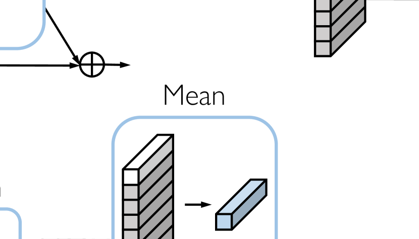
(a) $\mathtt{CB}$ Module

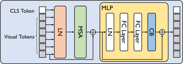
(b) Our Vision Transformer

Figure 4: Context Broadcasting ($\mathtt{CB}$) module. (a) Our $\mathtt{CB}$ module broadcasts the context to each token. (b) The $\mathtt{CB}$ module is inserted at the end of the $\mathtt{MLP}$ block of the Vision Transformer (ViT) architectures. ViTs have other possible positions for our module, but we analyze that inserting at the end of $\mathtt{MLP}$ outperforms others.

2.2 Explicitly Broadcasting the Context

We have observed certain hints for the benefit of additional spatial interaction and the fact that the uniform attention is the most challenging attention to learn from an optimization perspective. The observations motivate us to design a complementary operation that explicitly supplies the uniform attention. We do this through the broadcasting context with the $\mathtt{CB}$ module.

Context Broadcasting ($\mathtt{CB}$).

Given a sequence of $N$ tokens $\mathbf{X}\in\mathbb{R}^{N\times d}$, our $\mathtt{CB}$ module supplies the average-pooled token back onto the tokens as follows:

$$\mathtt{CB}({\mathbf{x}}_{i})=\frac{{\mathbf{x}}_{i}+\frac{1}{N}\sum_{j=1}^{N}{\mathbf{x}}_{j}}{2}\quad\text{for every token $i$},$$ (1)

where ${\mathbf{x}}_{i}\in\mathbb{R}^{d}$ is the $i^{\text{th}}$ token in $\mathbf{X}$. Figure 4(a) illustrates our $\mathtt{CB}$ module. The $\mathtt{CB}$ module is placed at the end of the multi-layer perceptron ($\mathtt{MLP}$) block. See Fig. 4(b) for the overall ViT architectures with our $\mathtt{CB}$ module. Our analysis in Sec. 3.1 shows that the insertion of $\mathtt{CB}$ increases the performance of ViTs regardless of its position. As we shall see, the performance increase is most significant when it is inserted after the $\mathtt{MLP}$ block.

Uniform attention helps.

To examine the effectiveness of the uniform attention, we conduct a preliminary experiment that directly injects the uniform attention into multi-head self-attention layers. We devise three ways of direct injection of the uniform attention to the layers: 1) We replace one of multi-head self-attention heads to be $\mathtt{CB}$ (denoted as Replc.) which reduces the number of parameters corresponding the replaced head, 2) we adjust the number of parameters of the Replc. way to be comparable to that of the original ViT (denoted as Comp.), and 3) we append $\mathtt{CB}$ to the multi-head self-attention as an extra head in parallel (denoted as Att.). Table 3 shows the top-1 accuracy according to the number of parameters. The three ways increase the accuracy by 0.2%p, 0.4%p, and 0.7%p, respectively. Compared to the above method, which add $\mathtt{CB}$ to $\mathtt{MLP}$, these settings are more direct ways to infuse the dense interactions into $\mathtt{MSA}$. Thus, the result explicitly tells us the broad benefits of injecting dense interactions to ViTs.

Computational efficiency.

The $\mathtt{CB}$ module is implemented with 1 line of code in deep learning frameworks like $\mathtt{PyTorch}$ (Paszke et al., 2019), $\mathtt{Tensorflow}$ (Abadi et al., 2016), and $\mathtt{JAX}$ (Bradbury et al., 2018): mygrayX = 0.5 * X + 0.5 * X.mean(dim=1, keepdim=True). It does not increase the number of parameters. It only incurs negligible additional operations for inference and training.

Dimension scaling.

Although we focus on a parameter-free way above, we propose a computationally efficient technique, dimension scaling, by introducing a minimal number of parameters. The proposed $\mathtt{CB}$ injects the dense interaction into all channel dimensions. Some channel dimensions of a token would require dense interaction, whereas others would not. We introduce the dimension scaling weights, $\mbox{\boldmath$\Lambda$}\in\mathbb{R}^{d}$, to infuse uniform attention selectively for each dimension as follows: $\mathtt{CB_{S}}({\mathbf{x}}_{i})={\mathbf{x}}_{i}+\mbox{\boldmath$\Lambda$}\odot\left(\frac{1}{N}\sum_{j=1}^{N}{\mathbf{x}}_{j}\right)$ where $\odot$ is the element-wise product. $\mathtt{CB_{S}}$ introduces few parameters: 0.02% additional parameters for ViT-S.

Table 1: ImageNet-1K performance of $\mathtt{CB}$ beside $\mathtt{MSA}$.

Module	# params [M]	Acc@1 [%]
ViT-S	22	79.9
Replc.	21	80.1 (+0.2)
Comp.	22	80.3 (+0.4)
Att.	29	80.6 (+0.7)

Table 2: Comparison with SE (Hu et al., 2018) and $\mathtt{CB}$.

Extra resources	SE	$\mathtt{CB}$
Parameter	Yes	No
Computation	High	Low
Implementation	Easy	One line

Table 3: ImageNet-1K performance of ViT-S with SE and $\mathtt{CB}$.

Module	Acc@1 [%]
ViT-S	79.9
+ SE	80.3 (+0.4)
+ $\mathtt{CB}$	80.5 (+0.6)

Comparison against SE.

The SE module (Hu et al., 2018) shares a certain similarity to $\mathtt{CB}$: both are modular attachments to neural network architecture and use pooling operations. However, SE (Hu et al., 2018) is designed for modeling the channel inter-dependency by exploiting pooling to construct channel descriptor, two FC layers, and a sigmoid function. Not only are the motivation and exact set of operations different, but also the computational requirements. See the comparison of additional computational costs for them in Table 3. $\mathtt{CB}$ is a much cheaper module to add than SE. Finally, we compare the performance of the models with SE and $\mathtt{CB}$ on ImageNet-1K in Table 3. Both modules improve the performance of ViT models, but the improvement is greater for $\mathtt{CB}$. Considering computational costs and accuracy improvements together, $\mathtt{CB}$ proves to be advantageous compared to SE.

3 Experiments

In Sec. 3.1, we experiment with which location we put our module in. In Secs. 3.2 and 3.3, we evaluate our modules on image classification (ImageNet-1K (Russakovsky et al., 2015)) and semantic segmentation (ADE20K (Zhou et al., 2017; 2019)) tasks. In Sec. 3.4, we show results on the robustness benchmarks, including occlusion, ImageNet-A (Hendrycks et al., 2021), and adversarial attack (Goodfellow et al., 2014). Finally, we conduct ablation studies such as entropy analysis, relative distance, scaling weights analysis, and the accuracy of varying heads in $\mathtt{MSA}$.

3.1 Where to Insert $\mathtt{CB}$ in a ViT

We study the best location for $\mathtt{CB}$ with respect to the main blocks for ViT architectures: $\mathtt{MSA}$ and $\mathtt{MLP}$. We train ViT-S with our module positioned on $\mathtt{MLP}$, $\mathtt{MSA}$, and both and validate on ImageNet-1K. As shown in Table 5, $\mathtt{CB}$ improves the performance regardless of blocks but achieves higher accuracy by 0.4%p in an $\mathtt{MLP}$ block than either in an $\mathtt{MSA}$ block or both. It is notable, though, that the addition of $\mathtt{CB}$ module increases the ViTs performance regardless of its location. We have chosen $\mathtt{MLP}$ as the default location of our $\mathtt{CB}$ module for the rest of the paper.

Now, we study the optimal position of the $\mathtt{CB}$ module within the $\mathtt{MLP}$ block. An $\mathtt{MLP}$ block consists of two fully-connected (FC) layers and the Gaussian Error Linear Unit (GELU) non-linear activation function (Hendrycks & Gimpel, 2016). Omitting the activation function for simplicity, we have three possible positions for $\mathtt{CB}$: $\mathtt{<Front>-FClayer-<Mid>-FClayer-<End>}$. We train ViT-S with $\mathtt{CB}$ located at $\mathtt{Front}$, $\mathtt{Mid}$, and $\mathtt{End}$ and validate on ImageNet-1K. Table 5 shows the results of the computation cost and top-1 accuracy. $\mathtt{Mid}$ and $\mathtt{End}$ increase accuracy by 0.6%p compared to the vanilla ViT-S. $\mathtt{Mid}$ demands four times larger computation costs than $\mathtt{End}$ because an $\mathtt{MLP}$ layer expands its channel dimensions four times rather than $\mathtt{Front}$ and $\mathtt{End}$. We conclude that inserting $\mathtt{CB}$ at $\mathtt{End}$ of $\mathtt{MLP}$ tends to produce the best results overall.

3.2 Image Classification

Settings.

ImageNet-1K (Russakovsky et al., 2015) consists of 1.28M training and 50K validation images with 1K classes. We train ViTs with our $\mathtt{CB}$ module on the training set and report accuracy on the validation set. For training ViTs on ImageNet-1K without other large datasets (Deng et al., 2009; Sun et al., 2017), we adopt strong regularizations following the DeiT (Touvron et al., 2021b) setting. We apply the random resized crop, random horizontal flip, Mixup (Zhang et al., 2018), CutMix (Yun et al., 2019), random erasing (Zhong et al., 2020), repeated augmentations (Hoffer et al., 2020), label-smoothing (Szegedy et al., 2016), and drop-path (Huang et al., 2016). We use AdamW (Loshchilov & Hutter, 2019) with betas of (0.9, 0.999), learning rate of $10^{-3}\cdot\mathrm{(batch\ size)}/1024$, and a weight decay of $0.05$. The one-cycle cosine scheduling is used to decay the learning rate during the total epochs of 300. We implement based on $\mathtt{PyTorch}$ (Paszke et al., 2019) and $\mathtt{timm}$ library (Wightman, 2019) on 8 V100 GPUs. We use $\mathtt{torchprofile}$ library to count the number of FLOPs. More details and additional experiments can be found in appendix.

Table 4: Experiments with the position of $\mathtt{CB}$. ImageNet-1K performance when $\mathtt{CB}$ is inserted to either $\mathtt{MLP}$ and $\mathtt{MSA}$ in ViT-S.

Module	Position		FLOPs [G]	Acc@1 [%]
	$\mathtt{MLP}$	$\mathtt{MSA}$
ViT-S	✗	✗	4.6	79.9
$\mathtt{CB}$	✓	✗	4.6	80.5 (+0.6)
	✗	✓	4.6	80.1 (+0.2)
	✓	✓	4.6	80.1 (+0.2)

Table 5: Experiments with the $\mathtt{CB}$ position in $\mathtt{MLP}$ block. ImageNet-1K performance when $\mathtt{CB}$ is placed at $\mathtt{Front}$, $\mathtt{Mid}$, or $\mathtt{End}$ in an $\mathtt{MLP}$ block.

Module	Position			FLOPs [G]	Acc@1 [%]
	$\mathtt{Front}$	$\mathtt{Mid}$	$\mathtt{End}$
ViT-S	✗	✗	✗	4.6	79.9
$\mathtt{CB}$	✓	✗	✗	4.6	79.9
	✗	✓	✗	4.6	80.5 (+0.6)
	✗	✗	✓	4.6	80.5 (+0.6)

Table 6: ImageNet-1K performance. We train transformer architectures with $\mathtt{CB}$ and $\mathtt{CB_{S}}$ and evaluate the accuracy on ImageNet-1K (Deng et al., 2009), ImageNet-V2 (Recht et al., 2019), and ImageNet-ReaL (Beyer et al., 2020). Green color denotes the performance gain against the original architecture.  indicates the models trained using the distillation loss (Touvron et al., 2021b).

Architecture	FLOPs [G]	Acc@1 [%]	Acc@5 [%]	IN-V2 [%]	IN-ReaL [%]
ViT-Ti	1.3	72.2	91.1	59.9	80.1
$+\ \mathtt{CB}$	1.3	73.2 (+1.0)	91.7 (+0.6)	60.9 (+1.0)	80.9 (+0.8)
$+\ \mathtt{CB_{S}}$	1.3	73.5 (+1.3)	91.9 (+0.8)	61.4 (+1.5)	81.2 (+1.1)
ViT-S	4.6	79.9	95.0	68.1	85.7
$+\ \mathtt{CB}$	4.6	80.5 (+0.6)	95.3 (+0.3)	69.3 (+1.2)	86.0 (+0.3)
$+\ \mathtt{CB_{S}}$	4.6	80.4 (+0.5)	95.1 (+0.1)	68.7 (+0.6)	85.9 (+0.2)
ViT-B	17.6	81.8	95.6	70.5	86.7
$+\ \mathtt{CB}$	17.6	82.0 (+0.2)	95.8 (+0.2)	70.6 (+0.1)	86.8 (+0.1)
$+\ \mathtt{CB_{S}}$	17.6	82.1 (+0.3)	95.8 (+0.2)	71.1 (+0.6)	86.9 (+0.2)
ViT-Ti	1.3	74.5	91.9	62.4	82.1
$+\ \mathtt{CB}$	1.3	74.7 (+0.2)	92.3 (+0.4)	62.5 (+0.1)	82.3 (+0.2)
$+\ \mathtt{CB_{S}}$	1.3	75.3 (+0.8)	92.5 (+0.6)	63.4 (+1.0)	82.8 (+0.7)
ViT-S	4.6	81.2	95.4	69.8	86.9
$+\ \mathtt{CB}$	4.6	81.3 (+0.1)	95.6 (+0.2)	70.2 (+0.4)	87.0 (+0.1)
$+\ \mathtt{CB_{S}}$	4.6	81.6 (+0.4)	95.6 (+0.2)	70.9 (+1.1)	87.3 (+0.4)
ViT-B	17.6	83.4	96.4	72.2	88.1
$+\ \mathtt{CB}$	17.6	83.5 (+0.1)	96.5 (+0.1)	72.3 (+0.1)	88.1
$+\ \mathtt{CB_{S}}$	17.6	83.6 (+0.2)	96.5 (+0.1)	73.4 (+1.2)	88.3 (+0.2)

Results. We train ViT-Ti/-S/-B (Dosovitskiy et al., 2021) with our module on ImageNet-1K and evaluate on validation of ImageNet-1K, ImageNet-V2 (Recht et al., 2019), and ImageNet-Real (Beyer et al., 2020). We follow the specification of ViT-Ti/-S from DeiT (Touvron et al., 2021b). As shown in Table 6, our modules $\mathtt{CB}$ and $\mathtt{CB_{S}}$ improve performance compared to the vanilla ViTs. $\mathtt{CB}$ does not change the number of parameters, and $\mathtt{CB_{S}}$ increases a few parameters. Our modules demand negligible computation costs compared to the original FLOPs. It shows that our modules are effective for image classification.

Table 7: ADE20K performance. All models are based on the UperNet (Xiao et al., 2018) model.

Backbone	# params [M]	mIoU [%]
		40K	160K
ViT-Ti	34.1	35.5	38.9
$+\ \mathtt{CB}$		36.5 (+1.0)	39.0 (+0.1)
$+\ \mathtt{CB_{S}}$		36.1 (+0.6)	39.8 (+0.9)
ViT-S	53.5	41.5	43.3
$+\ \mathtt{CB}$		41.9 (+0.4)	43.9 (+0.6)
$+\ \mathtt{CB_{S}}$		41.6 (+0.1)	43.1 (-0.2)
ViT-B	127.0	44.3	45.0
$+\ \mathtt{CB}$		45.1 (+0.8)	45.6 (+0.6)
$+\ \mathtt{CB_{S}}$		44.6 (+0.3)	45.3 (+0.3)

Table 8: Robustness evaluation. We evaluate ViT-S with $\mathtt{CB}$ and $\mathtt{CB_{S}}$ on center occlusion (Occ), ImageNet-A, and fast sign gradient method (FGSM) attack. Ours shows improved robustness across the board against ViT-S.

Architecture	Occ	ImageNet-A	FGSM
ViT-S	73.0	19.0	27.2
$+\ \mathtt{CB}$	74.0 (+1.0)	21.2 (+2.2)	32.3 (+5.1)
$+\ \mathtt{CB_{S}}$	73.7 (+0.7)	19.1 (+0.1)	27.8 (+0.6)

3.3 Semantic Segmentation

We validate our method for semantic segmentation on ADE20K dataset (Zhou et al., 2017; 2019), consisting of 20K training and 5K validation images. For a fair comparison, we follow the protocol of XCiT (El-Nouby et al., 2021) and Swin Transformer (Liu et al., 2021). We adopt UperNet (Xiao et al., 2018) and train for 40K iterations or 160K for longer training. Hyperparameters are the same as XCiT: the batch size of 16, AdamW with betas of (0.9, 0.999), the learning rate of $6\cdot 10^{-5}$, weight decay of 0.01, and polynomial learning rate scheduling. We set the head dimension as 192, 384, and 512 for ViT-Ti/-S/-B, respectively. Table 8 shows the results with 40K and 160K training settings. We observe that ViT-Ti/-S/-B with $\mathtt{CB}$ increase the mIoU by 1.0, 0.4, and 0.8 for 40K iterations and 0.1, 0.6, and 0.6 for 160K iterations, respectively. Similarly, $\mathtt{CB_{S}}$ improves mIoU except for 160K iterations in ViT-S. Infusing the context shows improvement in semantic segmentation.

3.4 Evaluating Model Robustness

We evaluate the robustness performance of $\mathtt{CB}$ and $\mathtt{CB_{S}}$ with respect to center occlusion (Occ), ImageNet-A (Hendrycks et al., 2021), and adversarial attack (Goodfellow et al., 2014). For Occ, we zero-mask the center $112\times 112$ patches of every validation image. ImageNet-A is the collection of challenging test images that an ensemble of ResNet50s has failed to recognize. We employ the fast sign gradient method (FGSM) for the adversarial attack. Table 8 shows the results of the robustness benchmark. $\mathtt{CB}$ increases 1.0, 2.2, and 5.1 of Occ, ImageNet-A, and FGSM, respectively; $\mathtt{CB_{S}}$ does 0.7, 0.1, and 0.6, respectively.

3.5 Ablation Study

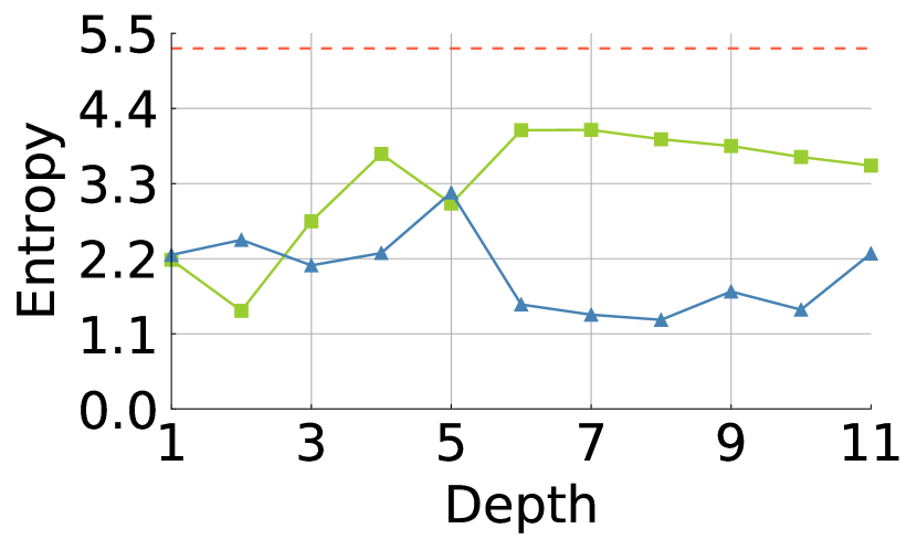
(a) Layer-wise entropy

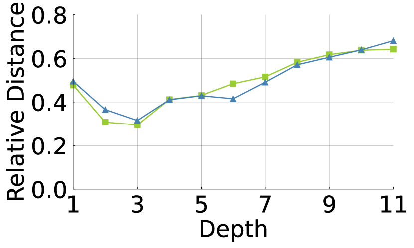
(b) Relative distance of attention

Figure 5: Attention entropy and relative distance. We visualize the averaged entropies of the class token and the relative distance of spatial interactions across the layers. The red dot line is the maximum value of entropy.

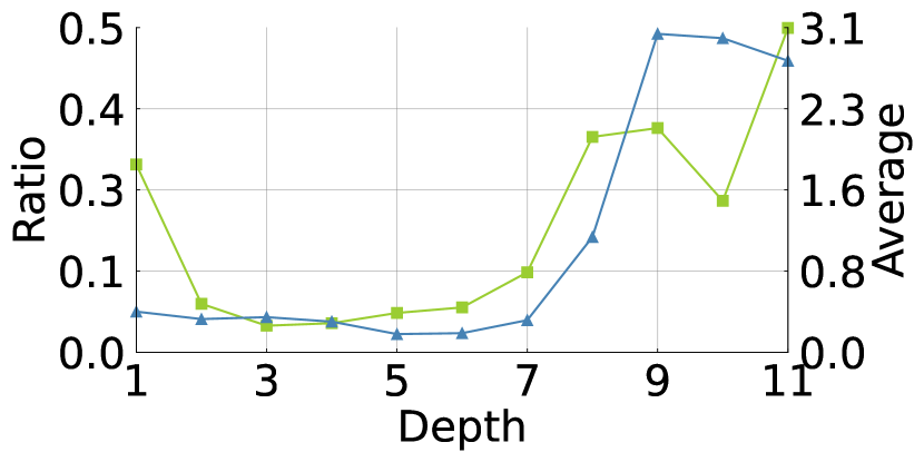
Figure 6: Analysis of dimension scaling. We plot values of ratio and average of scaling weights across the layers.

Model	No module	$\mathtt{CB}$	$\mathtt{CB}^{\dagger}$
ViT-Ti	72.2	73.2 (+1.0)	73.4 (+1.2)
ViT-S	79.9	80.5 (+0.6)	80.8 (+0.9)
ViT-B	81.8	82.0 (+0.2)	82.1 (+0.3)

Table 9: ImageNet-1K performance of $\mathtt{CB}$ at upper layers. We denote $\mathtt{CB}^{\dagger}$ as ViT-Ti/-S/-B with $\mathtt{CB}$ at the upper layers.

Figure 7:

ImageNet-1K performance with different number of heads.

We adjust the number of heads of ViT-Ti.

Attention entropy and relative distance according to the depth.

We have observed in Sec. 2.1 that the entropy of learned attention in ViT models tends to be high. From that, we have hypothesized that ViTs may benefit from an explicit injection of uniform attention. We examine now whether our $\mathtt{CB}$ module lowers the burden of the self-attention to learn dense interactions. We compare the entropy of the attention maps between ViT models with and without our $\mathtt{CB}$ module. Figure 5(a) shows layer-wise entropy values on ViT-S with and without our $\mathtt{CB}$ module. The insertion of $\mathtt{CB}$ module lowers the entropy values significantly, especially in deeper layers. It seems that $\mathtt{CB}$ relaxes the representational burden for the $\mathtt{MSA}$ block and lets it focus on sparse interactions.

We also observe that there exists a trend of increasing attention entropy in deeper ViT layers, as shown in Fig. 5(a). Inspired by this, we try inserting $\mathtt{CB}$ into only the deeper layers in a ViT model instead of the default mode of applying it to every layer. We denote this selective insertion method as $\mathtt{CB}^{\dagger}$. As shown in Table 9, $\mathtt{CB}^{\dagger}$ achieves 1.2%p, 0.9%p, and 0.3%p higher accuracy than the vanilla ViT-Ti/-S/-B, respectively. $\mathtt{CB}^{\dagger}$ also increases the top-1 accuracy further by 0.2%p, 0.3%p, and 0.1%p compared to ViT-Ti/-S/-B with $\mathtt{CB}$. We still believe the most practical solution is to apply $\mathtt{CB}$ to every layer. However, if the performance matters a lot, then one could also insert $\mathtt{CB}$ selectively to a subset of layers, particularly the deeper ones, for the best performance.

We compute the relative distance of spatial interactions to see whether $\mathtt{CB}$ affects the range of spatial interactions. We define the distance as follows: $\mathtt{dist}=E_{i\neq j,\{i,j\}\in[1,N]}(a_{ij}||{\mathbf{p}}_{i}-{\mathbf{p}}_{j}||_{1})$, where $N$ is the number of spatial tokens, $a_{ij}$ is the weight of attention between $i$-th and $j$-th tokens, and ${\mathbf{p}}_{i}$ is the normalized distance of $i$-th token. We exclude the case of self-interaction to analyze interactions of other tokens. As shown in Fig. 5(b), ViT-S and $\mathtt{CB}$ have a similar tendency. $\mathtt{CB}$ maintains the range of spatial interactions.

Analysis on dimension scaling.

We analyze the magnitude of scaling weights $\Lambda$ in $\mathtt{CB_{S}}$ to identify the tendency of the need for uniform attention according to depth. We measure the ratio of the quantile of $90\%$ and $10\%$, $|\lambda_{0.1}|/|\lambda_{0.9}|$. The ratio tells us how much high and low values of scaling weights are similar. We also compute the average of scaling weights according to depth. The average is related to the importance of uniform attention. As shown in Fig. 6, the ratio and average increase along with the depth. It means that the upper layers prefer dense interactions more than the lower layers. The result coincides with the above observation of entropy analysis.

Accuracy according to the number of heads.

$\mathtt{MSA}$ can model abundant spatial interactions between tokens as the number of attention heads increases. To examine the relationship between the number of heads and spatial interactions in $\mathtt{MSA}$, we train ViT-Ti with and without $\mathtt{CB}$ by adjusting the number of heads of $\mathtt{MSA}$. As shown in Fig. 7, the accuracy gap decreases as the number of heads increases. Our proposed module is, therefore, more effective in the lower number of heads rather than the large number of heads.

Table 10: Options for context aggregation. We consider replacing the averaging in $\mathtt{CB}$ with either max-pooling or the class token. We show ImageNet-1K top-1 accuracy on the validation set.

Architecture	Original	$\mathtt{CB}$ (Average)	Max-pooling	Class Token
ViT-S	79.9	80.5 (+0.6)	80.2 (+0.3)	79.3 ($-$0.6)

Other context broadcasting methods.

$\mathtt{CB}$ adds the averaged token but can adopt other aggregation methods than averaging in the pooling and context view. Global max pooling is another widely used method for generating the context. The class token in ViT architectures is another alternative for the source of context information; the class prediction is eventually performed with the class token. Table 10 lists the top-1 accuracy on ImageNet-1K validation set using max pooling or the class token. The max pooling improves the accuracy of ViT-S by 0.3%p but achieves a lower accuracy than our averaging in $\mathtt{CB}$. The replacement with the class token even decreases accuracy by 0.6%p. We suspect that it is because the value of the class token remains the same after the addition of the class token. Our averaging from the preliminary experiments in Sec. 2.1 outperforms the other simple context modelings.

4 Related Work

Transformers.

Since the seminal work of the Transformers (Vaswani et al., 2017), it has been the standard architecture in the natural language processing (NLP) domain. Dosovitskiy et al. (2021) have pioneered the use of Transformers in the visual domain with their Vision Transformers (ViTs). The way of ViTs work is almost identical to the original Transformers, where ViTs tokenize non-overlapping patches of the input image and apply the Transformers architecture on top.

There have been attempts to understand the algorithmic behaviors of ViTs, including $\mathtt{MSA}$, by contrasting them with CNNs (Raghu et al., 2021; Cordonnier et al., 2020; Naseer et al., 2021; Park & Kim, 2022; Tuli et al., 2021). Raghu et al. (2021) empirically demonstrate early aggregation of global information and much larger effective receptive fields (Luo et al., 2016) over CNNs. Naseer et al. (2021) show highly robust behaviors of ViTs against diverse nuisances, including occlusions, distributional shifts, adversarial and natural perturbations. Intriguingly, they attribute those advantageous properties to large and flexible receptive fields by $\mathtt{MSA}$ in ViTs and interactions therein. Similarly, there have been studies that attribute the effectiveness of $\mathtt{MSA}$ to global interaction in many visual scene understanding tasks (Carion et al., 2020; Strudel et al., 2021). In this work, we study the role of the density of the attention.

Attention module.

The global context is essential to capture a holistic understanding of a visual scene Torralba (2003); Rabinovich et al. (2007); Shotton et al. (2009); Wang et al. (2018); Cao et al. (to appear), which aids visual recognition. To capture the global context, models need to be designed to have sufficiently large receptive fields to interact and aggregate all the local information. Prior arts have proposed to enhance the interaction range of CNNs by going deeper (Simonyan & Zisserman, 2014; He et al., 2016) or by expanding the receptive fields (Yu & Koltun, 2016; Dai et al., 2017; Wang et al., 2018). Hu et al. (2018) squeeze spatial dimensions by pooling to capture the global context. Cao et al. (to appear) notice that the attention map of the non-local block is similar regardless of query position and propose a global context block. Different from our focus, the aforementioned methods focus on CNNs with additional learnable parameters.

5 Conclusion

We take a closer look at the spatial interactions in ViTs, especially in terms of density. We have been motivated by the exploration with a set of preliminary observations that suggest that ViT models prefer dense interactions. Incidentally, we also show that, at least from the optimization point of view, the uniform attention is perhaps the most difficult attention to learn. The preference and optimization difficulty of learning dense interactions are not harmonious. It leads us to introduce further dense interactions manually by a simple module: Context Broadcasting ($\mathtt{CB}$). Inserted at intermediate layers of ViT models, $\mathtt{CB}$ adds the average-pooled token to tokens. Additionally, we propose $\mathtt{CB}$ with the dimension scaling, $\mathtt{CB_{S}}$, to infuse the dense interactions selectively. Our simple modules turn out to improve the ViT performances across the board on image classification and semantic segmentation benchmarks. $\mathtt{CB}$ only takes 1 line of code, a few more FLOPs, and zero parameters to use this module. We hope this practical module could bring further performance boosts to your ViT models.

Reproducibility Statement

Training settings for classification and segmentation can be found in Secs. 3.2 and 3.3 (Also refer to Sec. A.3). The specifications of datasets used in experiments are in Sec. A.1. Additionally, our 1 line code implementation is attached in Secs. 2.2 and A.2.

Appendix

We present the experiment setup and additional experiments not included in the main paper. The contents of this appendix are listed as follows:

Contents

A    Details of Experiments Setup

  A.1    Datasets

  A.2    Models

  A.3    Hyper-parameters

B    Additional Experiments

  B.1    Training Curve

  B.2    Attention Visualization

  B.3    Other Architectures

  B.4    Robustness of ADE20K

  B.5    Discussion on Position of CB

  B.6    Utilizing The Class Token

 

Appendix A Details of Experiments Setup

This section provides license information of datasets and models used in the main paper with hyper-parameters of the training.

A.1 Datasets

ImageNet-1K. ImageNet-1K (Russakovsky et al., 2015) is the popular large-scale classification benchmark dataset, and the license is custom for research and non-commercial. ImageNet-1K consists of 1.28M training and 50K validation images with 1K classes. We use the training and the validation sets to train and evaluate architectures, respectively.

ImageNet-V2. ImageNet-V2 (Recht et al., 2019) is new test data for the ImageNet benchmark. Each of the three test sets in ImageNet-V2 comprises 10,000 new images. After a decade of progress on the original ImageNet dataset, these test sets were collected. This ensures that the accuracy scores are not influenced by overfitting and that the new test data is independent of existing models.

ImageNet-ReaL. ImageNet-ReaL (Beyer et al., 2020) develops a more reliable method for gathering annotations for the ImageNet validation set and is under the Apache 2.0 license. It re-evaluates the accuracy of previously proposed ImageNet classifiers using these new labels and finds their gains are smaller than those reported on the original labels. Therefore, this dataset is called the “Re-assessed Labels (ReaL)” dataset.

ADE20K. ADE20K (Zhou et al., 2017; 2019) is a semantic segmentation dataset, and the license is custom research-only and non-commercial. This contains over 20K scene-centric images that have been meticulously annotated with pixel-level objects and object parts labels. There are semantic categories, which encompass things like sky, road, grass, and discrete objects like person, car, and bed.

ImageNet-A. ImageNet-A (Hendrycks et al., 2021) is a set of images labeled with ImageNet labels that were created by collecting new data and preserving just the images that ResNet-50 (He et al., 2016) models failed to categorize properly. This dataset is under the MIT license. The label space is identical to ImageNet-1K.

A.2 Models

Dosovitskiy et al. (2021) have proposed ViT-B. Touvron et al. (2021b) have proposed the tiny and small ViT architectures named as ViT-Ti and ViT-S. The ViT architecture is similar to Transformer (Vaswani et al., 2017) but has patch embedding to make tokens of images. Specifically, ViT-Ti/-S/-B have 12 depth layers with 192, 384, and 768 dimensions, respectively. Heo et al. (2021) have proposed a variant of ViT by reducing the spatial dimensions and increasing the channel dimensions. ViTs consist of patch embedding layer, multi-head self-attention ($\mathtt{MSA}$) blocks, multi-layer perceptron ($\mathtt{MLP}$) blocks, and layer normalization ($\mathtt{LN}$) layers. As shown in Figure 8, our module is the modification of $\mathtt{MLP}$ block. Our module only requires 1 line modification at the end of the $\mathtt{MLP}$ layer.

⬇

1import torch.nn as nn

2

3class Mlp(nn.Module):

4 def __init__(self, in_features, hidden_features=None,

5 out_features=None, act_layer=nn.GELU, drop=0.):

6 super().__init__()

7 out_features = out_features or in_features

8 hidden_features = hidden_features or in_features

9 self.fc1 = nn.Linear(in_features, hidden_features)

10 self.act = act_layer()

11 self.fc2 = nn.Linear(hidden_features, out_features)

12 self.drop = nn.Dropout(drop)

13

14 def forward(self, x):

15 x = self.fc1(x)

16 x = self.act(x)

17 x = self.drop(x)

18 x = self.fc2(x)

19 x = self.drop(x)

20 return (x + x.mean(dim=1, keepdim=True)) * 0.5

Figure 8: Implementation of our $\mathtt{CB}$ module with PyTorch-like code. Our module requires 1 line modification at the end of the layer.

A.3 Hyper-parameters

Touvron et al. (2021b) have proposed data-efficient training setting with strong regularization such as MixUp (Zhang et al., 2018), CutMix (Yun et al., 2019), and random erasing (Zhong et al., 2020). We adopt the training setting of DeiT (Touvron et al., 2021b) and denote ViT-Ti/-S/-B with $\mathtt{CB}$ module. We do not use repeated augmentation for ViT-Ti/-S with ours. For ViT-B with ours, we increase the warmup-epochs from 5 to 10 and the drop-path. In distillation, we use the same hyper-parameters except for the drop-path of ViT-B with ours to 0.2.

Appendix B Additional Experiments

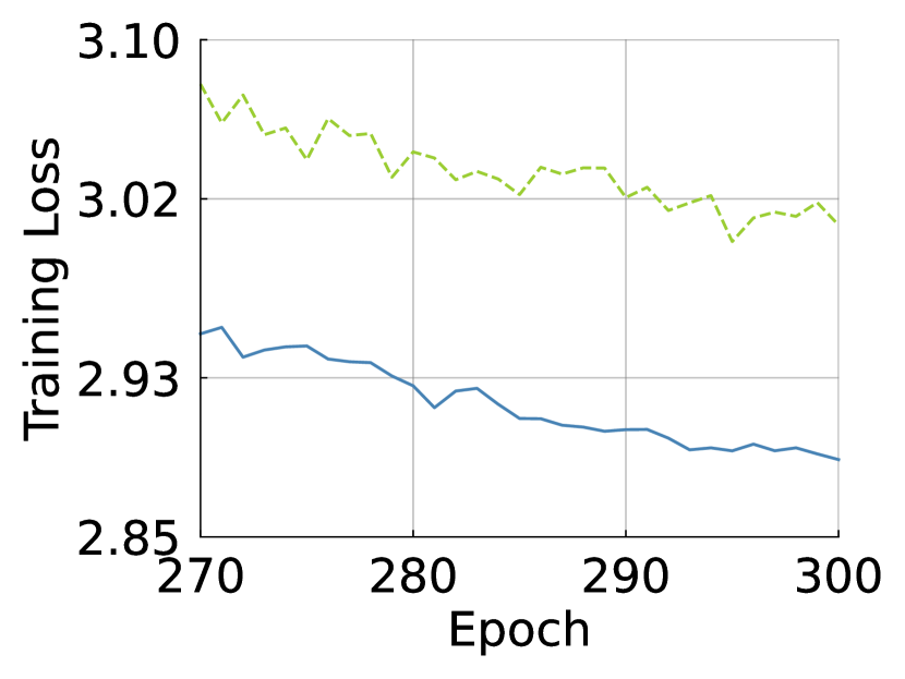
(a) Training Loss

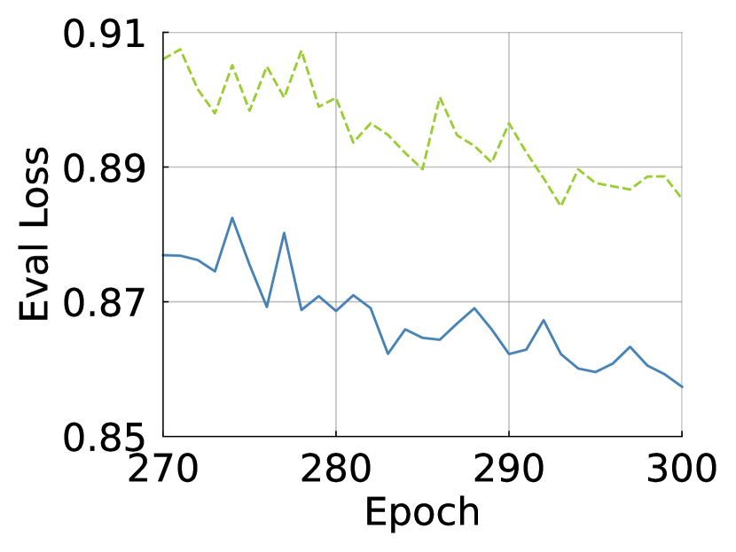
(b) Eval Loss

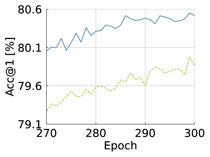
(c) Top-1 Accuracy

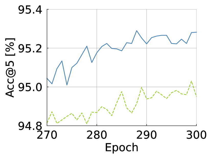
(d) Top-5 Accuracy

Figure 9: Training curve of ViT-S with and without $\mathtt{CB}$

B.1 Training Curve

We draw the training curve to see if $\mathtt{CB}$ improves the capacity of ViTs. As shown in Fig. 9, $\mathtt{CB}$ increase the top-1/-5 accuracies across epochs and decrease both training and evaluation losses more. This shows that $\mathtt{CB}$ improves the capacity of ViTs.

   

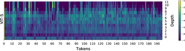
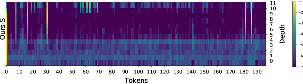
Figure 10: Visualization of attention corresponding with the class token. $x$-axis and $y$-axis represent tokens and depth. We denote ViT-S with $\mathtt{CB}$ as Ours-S. In ViT-S and Ours-S, the number of tokens and depth are 197 and 12, respectively; thus, the attention map is $12\times 197$. We apply the element-wise log operation to attention for visualization.

B.2 Attention Visualization

We visualize the attention of the class token to analyze how our $\mathtt{CB}$ module affects the ViT architecture. We utilize the pre-trained ViT-S with and without $\mathtt{CB}$ to extract values of attention. We denote ViT-S with $\mathtt{CB}$ as Ours-S. Figure 10 shows the attention map of the class token of randomly sampled images. $x$-axis and $y$-axis represent tokens and depth, respectively. We notice that the attention of Ours-S is more sparse than VIT-S in the upper layers. In Sec. 3.5, We have reported that the entropy is decreased when inserting $\mathtt{CB}$. The visualization and value of entropy have similar tendency. Our module reduces the density of the attention.

B.3 Other architectures

Table 11: ImageNet-1K performance on other architectures. We train PiT-B and MLP-Mixer architectures with $\mathtt{CB}$ and evaluate the accuracy on ImageNet-1K Deng et al. (2009).

Architecture	FLOPS [G]	Acc@1 [%]
PiT-B	12.4	82.0
$+\ \mathtt{CB}$	12.4	82.6 (+0.6)
$+\ \mathtt{CB_{S}}$	12.4	82.2 (+0.2)
Mixer-S/16	3.8	74.3
$+\ \mathtt{CB}$	3.8	74.9 (+0.6)

We evaluate $\mathtt{CB}$ on PiT (Heo et al., 2021) and Mixer (Tolstikhin et al., 2021). PiT-B is the variant of the original vision transformer by introducing spatial dimension reduction. Mixer is pioneering work of the feed-forward architectures (Tolstikhin et al., 2021; Touvron et al., 2021a), which mainly consist of FC layers. The structure of feed-forward architecture follows ViT except for $\mathtt{MSA}$. Spatial interactions of feed-forward are done by the transposing of visual data followed by an FC layer. We insert our module at $\mathtt{MLP}$ in PiT and Mixer (Tolstikhin et al., 2021). For a fair comparison, we reproduce the baseline Mixer-S/16 with the DeiT training regime (Touvron et al., 2021b) and train ours with the same one. Our module increases the performance of PiT-B and the vanilla Mixer-S/16 as shown in Table 11.

B.4 Robustness on ADE20K

Table 12: Robustness evaluation on ADE20K with input perturbations. We evaluate ViT-S with and without $\mathtt{CB}$ on Shot noise, Gaussian noise, and Gaussian blur. We run the experiments on random noise five times and report a mean with a confidence interval of 95%.

Noise Type	ViT-S	$\mathtt{CB}$
Nothing	43.3	43.9
Shot Noise	40.215 $\pm$ 0.151	41.088 $\pm$ 0.094
Gaussian Noise (sigma=5.0)	42.55 $\pm$ 0.0821	43.436 $\pm$ 0.0806
Gaussian Noise (sigma=10.0)	40.224 $\pm$ 0.065	41.068 $\pm$ 0.0591
Gaussian Blur (sigma=1.0)	42.29	43.26
Gaussian Blur (sigma=2.0)	40.83	41.44

We evaluate the robustness on ADE20K using input perturbations (Hendrycks & Dietterich, 2019), e.g., shot noise, Gaussian noise, and Gaussian blur. We run the experiments by five times on random noise and report the mean and confidence interval of 95%. Table 12 shows the performance of mIoU. The performance gap of ViT-S with and without $\mathtt{CB}$ increases from 0.6 up to 0.97. This shows our one line of code can improve the ViT models’ robustness against input perturbation in fine-tuning task.

B.5 Discussion on Position of $\mathtt{CB}$

We conclude the position of $\mathtt{CB}$ to the end of the $\mathtt{MLP}$ block by the observation in Sec. 3.1. We provide our intuition and discussion about the position of $\mathtt{CB}$ as follows:

Gradient signals

We think that the gradient signals are dependent on position. For simplicity, we assume a single layer composed of the $\mathtt{MSA}$ and $\mathtt{MLP}$ blocks.

• case 1, $\mathtt{<Front>}$: If $\mathtt{CB}$ is located at $\mathtt{<Front>}$, the subsequent weights in the corresponding $\mathtt{MLP}$ block cannot receive the gradient signals during training.

• case 2, $\mathtt{<End>}$: If $\mathtt{CB}$ is located at $\mathtt{<End>}$, the preceding weights in the $\mathtt{MLP}$ block are updated by the gradient signals by uniform attention.

Why is the improvement of $\mathtt{<Mid>}$ and $\mathtt{<End>}$ similar?

There is no non-linear function (e.g., GELU) between $\mathtt{<Mid>}$ and $\mathtt{<End>}$ positions. Since uniform attention is the addition of a globally averaged token, the output is identical wherever $\mathtt{CB}$ is located at $\mathtt{<Mid>}$ and $\mathtt{<End>}$. Therefore, the accuracy of both positions is similar. Nonetheless, $\mathtt{CB}$ at $\mathtt{<End>}$ achieves a bit higher top-5 accuracy than $\mathtt{CB}$ at $\mathtt{<Mid>}$ as shown in Table 5. As aforementioned, we suspect the $\mathtt{<End>}$ position provides the gradient induced by uniform attention to weights of the MLP block.

Table 13: Performance of ViT-S with $\mathtt{CB},\mathtt{CB}_{\texttt{gate}}$, and $\mathtt{CB}_{\texttt{hybrid}}$. We train ViT-S with $\mathtt{CB},\mathtt{CB}_{\texttt{gate}}$, and $\mathtt{CB}_{\texttt{hybrid}}$ on ImageNet-1K training set and evaluate top-1/-5 accuracy on the validation set. We vary the position of our modules at $\mathtt{MLP}$, $\mathtt{MSA}$, and both. Green color denotes the performance gain against the original architecture.

Module	Position		FLOPs [M]	Acc@1 [%]	Acc@5 [%]
	$\mathtt{MLP}$	$\mathtt{MSA}$
ViT-S	✗	✗	1260	79.9 (+0.0)	95.0 (+0.0)
$\mathtt{CB}$	✓	✗	+0.9	80.5 (+0.6)	95.3 (+0.3)
	✗	✓	+0.9	80.1 (+0.2)	95.0 (+0.0)
	✓	✓	+1.8	80.1 (+0.2)	95.0 (+0.0)
$\mathtt{CB}_{\texttt{gate}}$	✓	✗	+0.9	80.4 (+0.5)	95.1 (+0.1)
	✗	✓	+0.9	80.0 (+0.1)	95.0 (+0.0)
	✓	✓	+1.8	80.0 (+0.1)	95.0 (+0.0)
$\mathtt{CB}_{\texttt{hybrid}}$	✓	✗	+1.8	80.5 (+0.6)	95.0 (+0.0)
	✗	✓	+1.8	80.4 (+0.5)	95.3 (+0.3)
	✓	✓	+3.6	-	-

Table 14: Performance of ViT-S with different positions in $\mathtt{MLP}$ block. $\mathtt{MLP}$ has following schematic: $\mathtt{<Front>-FClayer-<Mid>-FClayer-<End>}$. We insert $\mathtt{CB},\mathtt{CB}_{\texttt{gate}}$, and $\mathtt{CB}_{\texttt{hybrid}}$ at $\mathtt{Front}$, $\mathtt{Mid}$, and $\mathtt{End}$ and evaluation on ImageNet-1K. Green and red colors denote the performance gain and drop against the original architecture.

Module	Position			FLOPS [M]	Acc@1 [%]	Acc@5 [%]
	$\mathtt{Front}$	$\mathtt{Mid}$	$\mathtt{End}$
ViT-S	✗	✗	✗	1260	79.9	95.0
$\mathtt{CB}$	✓	✗	✗	+0.9	79.9 (+0.0)	94.8 (–0.2)
	✗	✓	✗	+3.6	80.5 (+0.6)	95.2 (+0.2)
	✗	✗	✓	+0.9	80.5 (+0.6)	95.3 (+0.3)
$\mathtt{CB}_{\texttt{gate}}$	✓	✗	✗	+0.9	80.3 (+0.4)	94.9 (–0.1)
	✗	✓	✗	+3.6	80.2 (+0.3)	95.1 (+0.1)
	✗	✗	✓	+0.9	80.4 (+0.5)	95.1 (+0.1)
$\mathtt{CB}_{\texttt{hybrid}}$	✓	✗	✗	+1.8	80.5 (+0.6)	95.0 (+0.0)
	✗	✓	✗	+7.3	80.1 (+0.2)	95.1 (+0.1)
	✗	✗	✓	+1.8	80.3 (+0.4)	95.0 (+0.0)

B.6 Utilizing the class token

In Table 10, we do not see improvement by adding the class token and reason that the value of the class token remains the same from addition by itself. Since the class token evolves by interacting with entire tokens for tasks, we think that the class token could be utilized to complement spatial interactions of attention. We propose two additional baselines employing the class token.

The first one is the multiplication of the class token with each visual token, similar to the gating mechanism. We denote the first as $\mathtt{CB}_{\texttt{gate}}$ and formalize as follows: $\mathtt{CB}_{\texttt{gate}}({\mathbf{x}}_{i})={\mathbf{x}}_{i}({\mathbf{x}}_{0}+\mathbf{1})\text{ for every token $i$}$, where ${\mathbf{x}}_{0}$ is the class token and $\mathbf{1}$ is one vector. The second one is the combination of the class and average token denoted as $\mathtt{CB}_{\texttt{hybrid}}$: $\mathtt{CB}_{\texttt{hybrid}}({\mathbf{x}}_{i})={\mathbf{x}}_{i}{\mathbf{x}}_{0}+\mathtt{CB}({\mathbf{x}}_{i})\text{ for every token $i$}$. These modules are also parameter-free and computation efficient.

Firstly, we analyze the positions of $\mathtt{MLP}$ and $\mathtt{MSA}$. Table 13 lists FLOPs and validation accuracy of $\mathtt{MLP}$ and $\mathtt{MSA}$. Both $\mathtt{CB}_{\texttt{gate}}$ and $\mathtt{CB}_{\texttt{hybrid}}$ improve the top-1 accuracy regardless of positions except for the failure case of $\mathtt{CB}_{\texttt{hybrid}}$ at both $\mathtt{MLP}$ and $\mathtt{MSA}$ layers. These modules have the best top-1 accuracy at $\mathtt{MLP}$, consistent with our $\mathtt{CB}$ module.

We investigate different positions in an $\mathtt{MLP}$ layer with $\mathtt{CB}_{\texttt{gate}}$ and $\mathtt{CB}_{\texttt{hybrid}}$. Let the $\mathtt{MLP}$ layer consist as follows: $\mathtt{<Front>-FClayer-<Mid>-FClayer-<End>}$. Table 14 lists FLOPs and validation accuracy of $\mathtt{Front}$, $\mathtt{Mid}$, and $\mathtt{End}$. The best accuracy occurs at $\mathtt{End}$ for our $\mathtt{CB}$ module and $\mathtt{CB}_{\texttt{gate}}$ and $\mathtt{Front}$ for $\mathtt{CB}_{\texttt{hybrid}}$. At the best positions of respective modules, our $\mathtt{CB}$ module achieves 0.1%p higher accuracy than $\mathtt{CB}_{\texttt{gate}}$ and demands half of the FLOPs than $\mathtt{CB}_{\texttt{hybrid}}$.

Additionally, we can concatenate the pooled token instead of the addition. This operation increases the intermediate channel dimensions twice and requires additional projection layers. Since ViTs already have a large number of parameters and FLOPs, we focus on the parameter-free and operation-efficient module for uniform attention.

References

- Abadi et al. (2016) Martín Abadi, Paul Barham, Jianmin Chen, Zhifeng Chen, Andy Davis, Jeffrey Dean, Matthieu Devin, Sanjay Ghemawat, Geoffrey Irving, Michael Isard, et al. Tensorflow: A system for large-scale machine learning. In 12th USENIX Symposium on Operating Systems Design and Implementation (OSDI 16), 2016.
- Beyer et al. (2020) Lucas Beyer, Olivier J Hénaff, Alexander Kolesnikov, Xiaohua Zhai, and Aäron van den Oord. Are we done with imagenet? arXiv preprint arXiv:2006.07159, 2020.
- Bradbury et al. (2018) James Bradbury, Roy Frostig, Peter Hawkins, Matthew James Johnson, Chris Leary, Dougal Maclaurin, George Necula, Adam Paszke, Jake VanderPlas, Skye Wanderman-Milne, and Qiao Zhang. JAX: composable transformations of Python+NumPy programs, 2018. URL http://github.com/google/jax.
- Cao et al. (to appear) Yue Cao, Jiarui Xu, Stephen Lin, Fangyun Wei, and Han Hu. Global context networks. IEEE Transactions on Pattern Analysis and Machine Intelligence (TPAMI), to appear.
- Carion et al. (2020) Nicolas Carion, Francisco Massa, Gabriel Synnaeve, Nicolas Usunier, Alexander Kirillov, and Sergey Zagoruyko. End-to-end object detection with transformers. In European Conference on Computer Vision (ECCV), 2020.
- Cordonnier et al. (2020) Jean-Baptiste Cordonnier, Andreas Loukas, and Martin Jaggi. On the relationship between self-attention and convolutional layers. In International Conference on Learning Representations (ICLR), 2020.
- Dai et al. (2017) Jifeng Dai, Haozhi Qi, Yuwen Xiong, Yi Li, Guodong Zhang, Han Hu, and Yichen Wei. Deformable convolutional networks. In IEEE International Conference on Computer Vision (ICCV), 2017.
- Deng et al. (2009) Jia Deng, Wei Dong, Richard Socher, Li-Jia Li, Kai Li, and Li Fei-Fei. Imagenet: A large-scale hierarchical image database. In IEEE Conference on Computer Vision and Pattern Recognition (CVPR), 2009.
- Dosovitskiy et al. (2021) Alexey Dosovitskiy, Lucas Beyer, Alexander Kolesnikov, Dirk Weissenborn, Xiaohua Zhai, Thomas Unterthiner, Mostafa Dehghani, Matthias Minderer, Georg Heigold, Sylvain Gelly, Jakob Uszkoreit, and Neil Houlsby. An image is worth 16x16 words: Transformers for image recognition at scale. In International Conference on Learning Representations (ICLR), 2021.
- El-Nouby et al. (2021) Alaaeldin El-Nouby, Hugo Touvron, Mathilde Caron, Piotr Bojanowski, Matthijs Douze, Armand Joulin, Ivan Laptev, Natalia Neverova, Gabriel Synnaeve, Jakob Verbeek, and Herve Jegou. XCit: Cross-covariance image transformers. In Advances in Neural Information Processing Systems (NeurIPS), 2021.
- Goodfellow et al. (2014) Ian J Goodfellow, Jonathon Shlens, and Christian Szegedy. Explaining and harnessing adversarial examples. International Conference on Learning Representations (ICLR), 2014.
- He et al. (2016) Kaiming He, Xiangyu Zhang, Shaoqing Ren, and Jian Sun. Deep residual learning for image recognition. In IEEE Conference on Computer Vision and Pattern Recognition (CVPR), 2016.
- Hendrycks & Dietterich (2019) Dan Hendrycks and Thomas Dietterich. Benchmarking neural network robustness to common corruptions and perturbations. arXiv preprint arXiv:1903.12261, 2019.
- Hendrycks & Gimpel (2016) Dan Hendrycks and Kevin Gimpel. Gaussian error linear units (gelus). arXiv preprint arXiv:1606.08415, 2016.
- Hendrycks et al. (2021) Dan Hendrycks, Kevin Zhao, Steven Basart, Jacob Steinhardt, and Dawn Song. Natural adversarial examples. IEEE Conference on Computer Vision and Pattern Recognition (CVPR), 2021.
- Heo et al. (2021) Byeongho Heo, Sangdoo Yun, Dongyoon Han, Sanghyuk Chun, Junsuk Choe, and Seong Joon Oh. Rethinking spatial dimensions of vision transformers. In IEEE International Conference on Computer Vision (ICCV), 2021.
- Hoffer et al. (2020) Elad Hoffer, Tal Ben-Nun, Itay Hubara, Niv Giladi, Torsten Hoefler, and Daniel Soudry. Augment your batch: Improving generalization through instance repetition. In IEEE Conference on Computer Vision and Pattern Recognition (CVPR), 2020.
- Hu et al. (2018) Jie Hu, Li Shen, and Gang Sun. Squeeze-and-excitation networks. In IEEE Conference on Computer Vision and Pattern Recognition (CVPR), 2018.
- Huang et al. (2016) Gao Huang, Yu Sun, Zhuang Liu, Daniel Sedra, and Kilian Q Weinberger. Deep networks with stochastic depth. In European Conference on Computer Vision (ECCV), 2016.
- Liu et al. (2021) Ze Liu, Yutong Lin, Yue Cao, Han Hu, Yixuan Wei, Zheng Zhang, Stephen Lin, and Baining Guo. Swin transformer: Hierarchical vision transformer using shifted windows. In IEEE International Conference on Computer Vision (ICCV), 2021.
- Loshchilov & Hutter (2019) Ilya Loshchilov and Frank Hutter. Decoupled weight decay regularization. In International Conference on Learning Representations (ICLR), 2019.
- Luo et al. (2016) Wenjie Luo, Yujia Li, Raquel Urtasun, and Richard Zemel. Understanding the effective receptive field in deep convolutional neural networks. Advances in Neural Information Processing Systems (NeurIPS), 2016.
- Naseer et al. (2021) Muhammad Muzammal Naseer, Kanchana Ranasinghe, Salman H Khan, Munawar Hayat, Fahad Shahbaz Khan, and Ming-Hsuan Yang. Intriguing properties of vision transformers. In Advances in Neural Information Processing Systems (NeurIPS), 2021.
- Park & Kim (2022) Namuk Park and Songkuk Kim. How do vision transformers work? In International Conference on Learning Representations (ICLR), 2022.
- Paszke et al. (2019) Adam Paszke, Sam Gross, Francisco Massa, Adam Lerer, James Bradbury, Gregory Chanan, Trevor Killeen, Zeming Lin, Natalia Gimelshein, Luca Antiga, Alban Desmaison, Andreas Kopf, Edward Yang, Zachary DeVito, Martin Raison, Alykhan Tejani, Sasank Chilamkurthy, Benoit Steiner, Lu Fang, Junjie Bai, and Soumith Chintala. Pytorch: An imperative style, high-performance deep learning library. In Advances in Neural Information Processing Systems (NeurIPS), 2019.
- Rabinovich et al. (2007) Andrew Rabinovich, Andrea Vedaldi, Carolina Galleguillos, Eric Wiewiora, and Serge Belongie. Objects in context. In IEEE International Conference on Computer Vision (ICCV), 2007.
- Raghu et al. (2021) Maithra Raghu, Thomas Unterthiner, Simon Kornblith, Chiyuan Zhang, and Alexey Dosovitskiy. Do vision transformers see like convolutional neural networks? Advances in Neural Information Processing Systems (NeurIPS), 2021.
- Recht et al. (2019) Benjamin Recht, Rebecca Roelofs, Ludwig Schmidt, and Vaishaal Shankar. Do imagenet classifiers generalize to imagenet? In International Conference on Machine Learning (ICML), 2019.
- Russakovsky et al. (2015) Olga Russakovsky, Jia Deng, Hao Su, Jonathan Krause, Sanjeev Satheesh, Sean Ma, Zhiheng Huang, Andrej Karpathy, Aditya Khosla, Michael Bernstein, Alexander C. Berg, and Li Fei-Fei. ImageNet Large Scale Visual Recognition Challenge. International Journal of Computer Vision (IJCV), 2015.
- Shotton et al. (2009) Jamie Shotton, John Winn, Carsten Rother, and Antonio Criminisi. Textonboost for image understanding: Multi-class object recognition and segmentation by jointly modeling texture, layout, and context. International Journal of Computer Vision (IJCV), 81(1):2–23, 2009.
- Simonyan & Zisserman (2014) Karen Simonyan and Andrew Zisserman. Very deep convolutional networks for large-scale image recognition. In International Conference on Learning Representations (ICLR), 2014.
- Strudel et al. (2021) Robin Strudel, Ricardo Garcia, Ivan Laptev, and Cordelia Schmid. Segmenter: Transformer for semantic segmentation. In IEEE Conference on Computer Vision and Pattern Recognition (CVPR), 2021.
- Sun et al. (2017) Chen Sun, Abhinav Shrivastava, Saurabh Singh, and Abhinav Gupta. Revisiting unreasonable effectiveness of data in deep learning era. In IEEE International Conference on Computer Vision (ICCV), 2017.
- Szegedy et al. (2016) Christian Szegedy, Vincent Vanhoucke, Sergey Ioffe, Jon Shlens, and Zbigniew Wojna. Rethinking the inception architecture for computer vision. In IEEE Conference on Computer Vision and Pattern Recognition (CVPR), 2016.
- Tolstikhin et al. (2021) Ilya O Tolstikhin, Neil Houlsby, Alexander Kolesnikov, Lucas Beyer, Xiaohua Zhai, Thomas Unterthiner, Jessica Yung, Andreas Steiner, Daniel Keysers, Jakob Uszkoreit, et al. Mlp-mixer: An all-mlp architecture for vision. In Advances in Neural Information Processing Systems (NeurIPS), 2021.
- Torralba (2003) Antonio Torralba. Contextual priming for object detection. International Journal of Computer Vision (IJCV), 53(2):169–191, 2003.
- Touvron et al. (2021a) Hugo Touvron, Piotr Bojanowski, Mathilde Caron, Matthieu Cord, Alaaeldin El-Nouby, Edouard Grave, Gautier Izacard, Armand Joulin, Gabriel Synnaeve, Jakob Verbeek, et al. Resmlp: Feedforward networks for image classification with data-efficient training. arXiv preprint arXiv:2105.03404, 2021a.
- Touvron et al. (2021b) Hugo Touvron, Matthieu Cord, Matthijs Douze, Francisco Massa, Alexandre Sablayrolles, and Herve Jegou. Training data-efficient image transformers & distillation through attention. In International Conference on Machine Learning (ICML), 2021b.
- Tuli et al. (2021) Shikhar Tuli, Ishita Dasgupta, Erin Grant, and Thomas L Griffiths. Are convolutional neural networks or transformers more like human vision? arXiv preprint arXiv:2105.07197, 2021.
- Vaswani et al. (2017) Ashish Vaswani, Noam Shazeer, Niki Parmar, Jakob Uszkoreit, Llion Jones, Aidan N Gomez, Ł ukasz Kaiser, and Illia Polosukhin. Attention is all you need. In Advances in Neural Information Processing Systems (NeurIPS), 2017.
- Wang et al. (2018) Xiaolong Wang, Ross Girshick, Abhinav Gupta, and Kaiming He. Non-local neural networks. In IEEE Conference on Computer Vision and Pattern Recognition (CVPR), 2018.
- Wightman (2019) Ross Wightman. Pytorch image models. https://github.com/rwightman/pytorch-image-models, 2019.
- Xiao et al. (2018) Tete Xiao, Yingcheng Liu, Bolei Zhou, Yuning Jiang, and Jian Sun. Unified perceptual parsing for scene understanding. In European Conference on Computer Vision (ECCV), 2018.
- Yu & Koltun (2016) Fisher Yu and Vladlen Koltun. Multi-scale context aggregation by dilated convolutions. In International Conference on Learning Representations (ICLR), 2016.
- Yun et al. (2019) Sangdoo Yun, Dongyoon Han, Seong Joon Oh, Sanghyuk Chun, Junsuk Choe, and Youngjoon Yoo. Cutmix: Regularization strategy to train strong classifiers with localizable features. In IEEE International Conference on Computer Vision (ICCV), 2019.
- Zhang et al. (2018) Hongyi Zhang, Moustapha Cisse, Yann N. Dauphin, and David Lopez-Paz. mixup: Beyond empirical risk minimization. In International Conference on Learning Representations (ICLR), 2018.
- Zhong et al. (2020) Zhun Zhong, Liang Zheng, Guoliang Kang, Shaozi Li, and Yi Yang. Random erasing data augmentation. In AAAI Conference on Artificial Intelligence (AAAI), 2020.
- Zhou et al. (2017) Bolei Zhou, Hang Zhao, Xavier Puig, Sanja Fidler, Adela Barriuso, and Antonio Torralba. Scene parsing through ade20k dataset. In IEEE Conference on Computer Vision and Pattern Recognition (CVPR), 2017.
- Zhou et al. (2019) Bolei Zhou, Hang Zhao, Xavier Puig, Tete Xiao, Sanja Fidler, Adela Barriuso, and Antonio Torralba. Semantic understanding of scenes through the ade20k dataset. International Journal of Computer Vision (IJCV), 127(3):302–321, 2019.