CLEAR: Generative Counterfactual Explanations
on Graphs

Abstract

Counterfactual explanations promote explainability in machine learning models by answering the question “how should an input instance be perturbed to obtain a desired predicted label?". The comparison of this instance before and after perturbation can enhance human interpretation. Most existing studies on counterfactual explanations are limited in tabular data or image data. In this work, we study the problem of counterfactual explanation generation on graphs. A few studies have explored counterfactual explanations on graphs, but many challenges of this problem are still not well-addressed: 1) optimizing in the discrete and disorganized space of graphs; 2) generalizing on unseen graphs; and 3) maintaining the causality in the generated counterfactuals without prior knowledge of the causal model. To tackle these challenges, we propose a novel framework CLEAR which aims to generate counterfactual explanations on graphs for graph-level prediction models. Specifically, CLEAR leverages a graph variational autoencoder based mechanism to facilitate its optimization and generalization, and promotes causality by leveraging an auxiliary variable to better identify the underlying causal model. Extensive experiments on both synthetic and real-world graphs validate the superiority of CLEAR over the state-of-the-art methods in different aspects.

1 Introduction

To facilitate explainability in opaque machine learning (ML) models (e.g., how predictions are made by a model, and what to do to achieve a desired outcome), explainable artificial intelligence (XAI) linardatos2020explainable has recently attracted significant attention in many communities. Among the existing work of XAI, a special class, i.e., counterfactual explanation (CFE) wachter2017counterfactual , promotes model explainability by answering the following question: “For a specific instance, how should the input features $X$ be slightly perturbed to new features $X^{\prime}$ to obtain a different predicted label (often a desired label) from ML models?". The original instance whose prediction needs to be explained is called an explainee instance, and the generated instances after perturbation are referred to as “counterfactual explanations". Generally, CFE promotes human interpretation through the comparison between $X$ and $X^{\prime}$. With its intuitive nature, CFEs can be deployed in various real-world scenarios such as loan application and legal framework verma2020counterfactual . Different from traditional CFE studies wachter2017counterfactual ; verma2020counterfactual ; mahajan2019preserving ; mishra2021survey on tabular or image data, recently, CFE on graphs is also an emerging field in many domains with graph structure data such as molecular analysis numeroso2021meg and professional networking wolff2009effects . For example, consider a grant application prediction grant model with each input instance as a graph representing a research team’s collaboration network, where each node represents a team member, and each edge signifies a collaboration relationship between them. Team leaders can improve their teams for next application by changing the original graph according to the counterfactual with a desired predicted label (application being granted). If the counterfactual is more dense than the original, the team leader may then encourage more team collaborations. To this end, in this work, we investigate the problem of generating counterfactual explanations on graphs. As shown in Fig. 1, given a prediction model $f$ on graphs, for a graph instance $G$, we aim to generate counterfactuals (e.g., $G^{CF}$) which are slightly different from $G$ w.r.t. their node features or graph structures to elicit a desired model prediction. Specifically, we focus on graph-level prediction without any assumptions of the prediction model type and its model access, i.e., $f$ can be a black box with unknown structure.

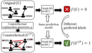
Figure 1: An example of CFE on graphs.

Recently, a few studies lucic2021cf ; numeroso2021meg ; bajaj2021robust ; abrate2021counterfactual ; ying2019gnnexplainer ; yuan2020explainability explore to extend CFEs into graphs. However, this problem still remains a daunting task due to the following key challenges: 1) Optimization: Different from traditional data, the space of perturbation operations on graphs (e.g., add/remove nodes/edges) is discrete, disorganized, and vast, which brings difficulties for optimization in CFE generation. Most existing methods numeroso2021meg ; abrate2021counterfactual search for graph counterfactuals by enumerating all the possible perturbation operations on the current graph. However, such enumeration on graphs is of high complexity, and it is also challenging to solve an optimization problem in such a complex search space. Few graph CFE methods which enable gradient-based optimization either rely on domain knowledge numeroso2021meg or assumptions bajaj2021robust about the prediction model to facilitate optimization. However, these knowledge and assumptions limit their applications in different scenarios. 2) Generalization: The discrete and disorganized nature of graphs also brings challenges for the generalization of CFE methods on unseen graphs, as it is hard to sequentialize the process of graph CFE generation and then generalize it. Most existing CFE methods on graphs lucic2021cf ; ying2019gnnexplainer solve an optimization problem for each explainee graph separately. These methods, however, cannot be generalized to new graphs. 3) Causality: It is challenging to generate counterfactuals that are consistent with the underlying causality. Specifically, causal relations may exist among different node features and the graph structure. In the aforementioned example, for each team, after establishing more collaborations, the team culture may be causally influenced. Incorporating causality can generate more realistic and feasible counterfactuals mahajan2019preserving , but most existing CFE methods either cannot handle causality, or require too much prior knowledge about the causal relations in data.

To address the aforementioned challenges, in this work, we propose a novel framework — generative CounterfactuaL ExplAnation geneRator for graphs (CLEAR). At a high level, CLEAR is a generative, model-agnostic CFE generation framework for graph prediction models. For any explainee graph instance, CLEAR aims to generate counterfactuals with slight perturbations on the explainee graph to elicit a desired predicted label, and the counterfactuals are encouraged to be in line with the underlying causality. More specifically, to facilitate the optimization of the CFE generator, we map each graph into a latent representation space, and output the counterfactuals as a probabilistic fully-connected graph with node features and graph structure similar as the explainee graph. In this way, the framework is differentiable and enables gradient-based optimization. To promote generalization of the CFE generator on unseen graphs, we propose a generative way to construct the counterfactuals. After training the CFE generator, it can be efficiently deployed to generate (multiple) counterfactuals on unseen graphs, rather than retraining from scratch. To generate more realistic counterfactuals without explicit prior knowledge of the causal relations, inspired by the recent progress in nonlinear independent component analysis (ICA) khemakhem2020variational and its connection with causality pearl2009causality , we make an exploration to promote causality in counterfactuals by leveraging an auxiliary variable to better identify the latent causal relations. The main contributions of this work can be summarized as follows: 1) Problem. We study an important problem: counterfactual explanation generation on graphs. We analyze its challenges including optimization, generalization, and causality. To the best of our knowledge, this is the first work jointly addressing all these challenges of this problem. 2) Method. We propose a novel framework CLEAR to generate counterfactual explanations for graphs. CLEAR can generalize to unseen graphs, and promote causality in the counterfactuals. 3) Experiments. We conduct extensive experiments on both synthetic and real-world graphs to validate the superiority of our method over state-of-the-art baselines of graph CFE generation.

2 Preliminaries

A graph $G=(X,A)$ is specified with its node feature $X$ and adjacency matrix $A$. We have a graph prediction model $f:\mathcal{G}\rightarrow\mathcal{Y}$, where $\mathcal{G}$ and $\mathcal{Y}$ represent the space of graphs and labels, respectively. In this work, we assume that we can access the prediction of $f$ for any input graph, but we do not assume the access of any knowledge of the prediction model itself. For a graph $G\in\mathcal{G}$, we denote the output of the prediction model as $Y=f(G)$. A counterfactual $G^{CF}=(X^{CF},A^{CF})$ is expected to be similar as the original explainee graph $G$, but the predicted label for $G^{CF}$ made by $f$ (i.e., $Y^{CF}=f(G^{CF})$) should be different from $f(G)$. With a desired label $Y^{*}$ (here $Y^{*}\neq Y$), the counterfactual $G^{CF}$ is considered to be valid if and only if $Y^{*}=Y^{CF}$. In this paper, we mainly focus on graph classification, but our framework can also be extended to other tasks such as node classification, as discussed in Appendix D.

Suppose we have a set of graphs sampled from the space $\mathcal{G}$, and different graphs may have different numbers of nodes and edges. A counterfactual explanation generator can generate counterfactuals for any input graph $G$ w.r.t. its desired predicted label $Y^{*}$. As aforementioned, most existing CFE methods on graphs have limitations in three aspects: optimization, generalization, and causality. Next, we provide more background of causality. The causal relations between different variables (e.g., node features, degree, etc.) in the data can be described with a structural causal model (SCM):

Definition 1.

(Structural Causal Model) A structural causal model (SCM) pearl2009causality is denoted by a triple $(U,V,F)$: $U$ is a set of exogenous variables, and $V$ is a set of endogenous variables. The structural equations $F\!=\!\{F_{1},...,F_{|V|}\}$ determine the value for each $V_{i}\!\in\!V$ with $V_{i}\!=\!F_{i}(\mathtt{PA}_{i},U_{i})$, here $\mathtt{PA}_{i}\!\subseteq\!{V}\backslash V_{i}$ denotes the “parents" of $V_{i}$, and $U_{i}\!\subseteq\!U$.

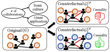
Figure 2: An example of causality in CFE.

Definition 2.

(Causality in CFE) For an explainee graph $G$, a counterfactual $G^{CF}$ satisfies causality if the change from $G$ to $G^{CF}$ is consistent with the underlying structural causal model.

Example: In the aforementioned grant application example, for a research team which has been rejected for an application before (as the graph $G$ in Fig. 2), to get the next application approved, a valid counterfactual may suggest this team to improve the number of collaborations between team members. Based on real-world observations, we assume that an additional causal relation exists: the number of team collaborations causally affects the team culture. For example, for the same team, if more collaborations had been established, then the team culture should have been improved in terms of better member engagement and respect for diversity. The SCM is illustrated in Fig. 2, where we leave out the exogenous variables for simplicity. Although the team culture usually does not affect the result of grant application, the counterfactuals with team culture changed correspondingly when the number of collaborations changes are more consistent with the ground-truth SCM. $G^{CF}_{2}$ in Fig. 2 shows an example of such counterfactuals. In contrast, if a counterfactual improves a team’s number of collaborations alone without improving the team culture (see $G^{CF}_{1}$ in Fig. 2), then it violates the causality. As discussed in mahajan2019preserving , traditional CFE methods often optimize on a single instance, and are prone to perturb different features independently, thus they often fail to satisfy the causality.

3 The Proposed Framework — CLEAR

In this section, we describe a novel generative framework — CLEAR, which addresses the problem of counterfactual explanation generation for graphs. First, we introduce its backbone CLEAR-VAE to enable optimization on graphs and generalization on unseen graph instances. This backbone is based on a graph variational auto-encoder (VAE) simonovsky2018graphvae mechanism. On top of CLEAR-VAE, we then promote the causality of CFEs with an auxiliary variable.

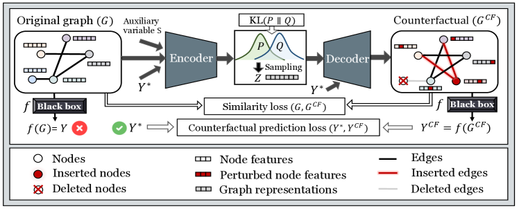
Figure 3: An illustration of the proposed framework CLEAR.

3.1 CLEAR-VAE: Backbone of Graph Generative Counterfactual Explanations

Different from most existing methods lucic2021cf ; ying2019gnnexplainer for CFE generation on graphs which focus on a single graph instance, CLEAR is based on a generative backbone CLEAR-VAE which can efficiently generate CFEs for different graphs after training, even for the graphs that do not appear in the training data. As shown in Fig. 3, CLEAR-VAE follows a traditional graph VAE simonovsky2018graphvae architecture with an encoder and a decoder. The encoder maps each original graph $G=(X,A)$ into a latent space as a representation $Z$, then the decoder generates a counterfactual $G^{CF}$ based on the latent representation $Z$. Following the VAE mechanism as in simonovsky2018graphvae ; kingma2013auto and its recent application in CFE generation for tabular data mahajan2019preserving ; pawelczyk2020learning , the optimization objective is based on the evidence lower bound (ELBO), which is a lower bound for the log likelihood $\ln P(G^{CF}|Y^{*},G)$. Here, $P(G^{CF}|Y^{*},G)$ is the probability of the generated counterfactual $G^{CF}$ conditioned on an input explainee graph $G$ and a desired label $Y^{*}$. The ELBO for CLEAR-VAE can be derived as follows:

$$\begin{split}\ln P(G^{CF}|Y^{*},G)\geq\mathbb{E}_{Q}[\ln P(G^{CF}|Z,Y^{*},G)]-\text{KL}(Q(Z|G,Y^{*})\|P(Z|G,Y^{*})),\end{split}$$ (1)

where $Q$ refers to the approximate posterior distribution $Q(Z|G,Y^{*})$, and $\text{KL}(\cdot||\cdot)$ means the Kullback-Leibler (KL) divergence. The first term $P(G^{CF}|Z,Y^{*},G)$ denotes the probability of the generated counterfactual conditioned on the representation $Z$ and the desired label $Y^{*}$. Due to the lack of ground-truth counterfactuals, it is hard to directly optimize this term. But inspired by mahajan2019preserving , maximizing this term can be considered as generating valid graph counterfactuals w.r.t. the desired label $Y^{*}$, thus we replace this term with $-\mathbb{E}_{Q}[d(G,G^{CF})+\alpha\cdot l(f(G^{CF}),Y^{*})],$ where $d(\cdot,\cdot)$ is a similarity loss, which is a distance metric to measure the difference between $G$ and $G^{CF}$, $l(\cdot)$ is the counterfactual prediction loss to measure the difference between the predicted label $f(G^{CF})$ and the desired label $Y^{*}$. In summary, these two terms encourage the model to output counterfactuals which are similar as the input graph but elicit the desired predicted label. $\alpha$ is a hyperparameter to control the weight of the counterfactual prediction loss. Overall, the loss function of CLEAR-VAE is:

$$\begin{split}\mathcal{L}=\mathbb{E}_{Q}[d(G,G^{CF})+\alpha\cdot l(f(G^{CF}),Y^{*})]+\text{KL}(Q(Z|G,Y^{*})\|P(Z|G,Y^{*})).\end{split}$$ (2)

Encoder. In the encoder, the input includes node features $X$ and graph structure $A$ of the explainee graph $G$, as well as the desired label $Y^{*}$, the output is latent representation $Z$. The encoder learns the distribution $Q(Z|G,Y^{*})$. We use a Gaussian distribution $P(Z|G,Y^{*})=\mathcal{N}(\mu_{z}({Y^{*})},\text{diag}(\sigma^{2}_{z}{(Y^{*}))})$ as prior, and enforce the learned distribution $Q(Z|G,Y^{*})$ to be close to the prior by minimizing their KL divergence. Here, $\mu_{z}({Y^{*})}$ and $\text{diag}(\sigma^{2}_{z}(Y^{*}))$ are mean and diagonal covariance of the prior distribution learned by a neural network module. $Z$ is sampled from the learned distribution $Q(Z|G,Y^{*})$ with the widely-used reparameterization trick kingma2013auto .

Decoder. In the decoder, the input includes $Z$ and $Y^{*}$, while the output is the counterfactual $G^{CF}=(X^{CF},A^{CF})$. Different counterfactuals can be generated for one explainee graph by sampling $Z$ from $Q(Z|G,Y^{*})$ for multiple times. The adjancency matrix is often discrete, and typically assumed to include only binary values ($A_{(i,j)}=1$ if edge from node $i$ to node $j$ exists, otherwise $A_{(i,j)}=0$). To facilitate optimization, inspired by recent graph generative models lucic2021cf ; simonovsky2018graphvae , our decoder outputs a probabilistic adjacency matrix $\hat{A}^{CF}$ with elements in range $[0,1]$, and then generates a binary adjancency matrix $A^{CF}$ by sampling from Bernoulli distribution with probabilities in $\hat{A}^{CF}$. We calculate the similarity loss in Eq. (2) as:

$$d(G,G^{CF})=d_{A}({A},\hat{A}^{CF})+\beta\cdot d_{X}({X},X^{CF}),$$ (3)

where $d_{A}$ and $d_{X}$ are metrics to measure the distance between two graphs w.r.t. their graph structures and node features, respectively. $\beta$ controls the weight for the similarity loss w.r.t. node features. More details of model implementation are in Appendix B.

3.2 CLEAR: Improving the Causality in Counterfactual Explanations

To further incorporate the causality in the generated CFEs, most existing studies mahajan2019preserving ; karimi2020algorithmic ; karimi2021algorithmic leverage certain prior knowledge (e.g., a given path diagram which depicts the causal relations among variables) of the SCM. However, it is often difficult to obtain sufficient prior knowledge of the SCM in real-world data, especially for graph data. In this work, we do not assume the access of the prior knowledge of SCM, and only assume that the observational data is available. However, the key challenge, as shown in karimi2020algorithmic , is that it is impossible to identify the ground-truth SCM from observational data without additional assumptions w.r.t. the structural equations and the exogenous variables, because different SCMs may result in the same observed data distribution. Considering that different SCMs can generate different counterfactuals, the identifiability of SCM is an obstacle of promoting causality in CFE. Fortunately, enlightened by recent progress in nonlinear independent component analysis (ICA) khemakhem2020variational ; hyvarinen2019nonlinear , we make an initial exploration to promote causality in CFE by improving the identifiability of the latent variables in our CFE generator with the help of an auxiliary observed variable. This CFE generator is denoted by CLEAR.

In nonlinear independent component analysis (ICA) khemakhem2020variational ; hyvarinen2019nonlinear ; shimizu2006linear ; monti2020causal , it is assumed that the observed data, e.g., $X$, is generated from a smooth and invertible nonlinear transformation of independent latent variables (referred to as sources) $Z$. Identifying the sources and the transformation are the key goals in nonlinear ICA. Similarly, traditional VAE models also assume that the observed features $X$ are generated by a set of latent variables $Z$. However, traditional VAEs cannot be directly used for nonlinear ICA as they lack identifiability, i.e., we can find different $Z$ that lead to the same observed data distribution $p(X)$. Recent studies khemakhem2020variational have shown that the identifiability of VAE models can be improved with an auxiliary observed variable $S$ (e.g., a time index or class label), which enables us to use VAE for nonlinear ICA problem. As discussed in shimizu2006linear ; monti2020causal , a SCM can be considered as a nonlinear ICA model if the exogenous variables in the SCM are considered as the sources in nonlinear ICA. Similar connections can be built between the structural equations in SCM and the transformations in ICA. Such connections shed a light on improving the identifiability of the underlying SCM without much explicit prior knowledge of the SCM.

With this idea, based on the backbone CLEAR-VAE, CLEAR improves the causality in counterfactuals by promoting identifiability with an observed auxiliary variable $S$. Intuitively, we expect the graph VAE can capture the exogenous variables of the SCM in its representations $Z$, and approximate the data generation process from the exogenous variables to the observed data, which is consistent with the SCM. Here, for each graph, the auxiliary variable $S$ can provide additional information for CLEAR to better identify the exogenous variables in the SCM, and thus can elicit counterfactuals with better causality. To achieve this goal, following the previous work of nonlinear ICA khemakhem2020variational ; hyvarinen2019nonlinear , we make the following assumption:

Assumption 1.

We assume that the prior on the latent variables $P(Z|S)$ is conditionally factorial.

With this assumption, the original data can be stratified by different values of $S$, and each separated data stratum can be considered to be generated by the ground-truth SCM under certain constraints (e.g., the range of values that the exogenous variables can take). When the constraints become more restricted, the space of possible SCMs that can generate the same data distribution in each data stratum shrinks. In this way, the identification of the ground-truth SCM can be easier if we leverage the auxiliary variable $S$. Here, with the auxiliary variable $S$, we infer the ELBO of CLEAR:

Theorem 1. The evidence lower bound (ELBO) to optimize the framework CLEAR is:

$$\begin{split}\ln P(G^{CF}|S,Y^{*},G)\geq\mathbb{E}_{Q}[\ln P(G^{CF}|Z,S,Y^{*},G)]\!-\!\text{KL}(Q(Z|G,S,Y^{*})\|P(Z|G,S,Y^{*})),\end{split}$$ (4)

the detailed proof is shown in Appendix A.

Loss function of CLEAR. Based on the above ELBO, the final loss function of CLEAR is:

$$\begin{split}\mathcal{L}=\,\mathbb{E}_{Q}[d(G,G^{CF})+\alpha\cdot l(f(G^{CF}),Y^{*})]+\text{KL}(Q(Z|G,S,Y^{*})\|P(Z|G,S,Y^{*})).\end{split}$$ (5)

Encoder and Decoder. The encoder takes the input $G$, $S$, and $Y^{*}$, and outputs $Z$ as the latent representation. We use a Gaussian prior $P(Z|G,S,Y^{*})=\mathcal{N}(\mu_{z}{(S,Y^{*})},\text{diag}(\sigma^{2}_{Z}{(S,Y^{*})})$ with its mean and diagonal covariance learned by neural network, and we encourage the learned approximate posterior $Q(Z|G,S,Y^{*})$ to approach the prior by minimizing their KL divergence. Similar to the backbone CLEAR-VAE, the decoder takes the inputs $Z$ and $Y^{*}$ to generate one or multiple counterfactuals $G^{CF}$ for each explainee graph. More implementation details are in Appendix B.

4 Experiment

In this section, we evaluate our framework CLEAR  with extensive experiments on both synthetic and real-world graphs. In particular, we answer the following research questions in our experiments: RQ1: How does CLEAR perform compared to state-of-the-art baselines? RQ2: How do different components in CLEAR contribute to the performance? RQ3: How can the generated CFEs promote model explainability? RQ4: How does CLEAR perform under different settings of hyperparameters?

4.1 Baselines

We use the following baselines for comparison: 1) Random: For each explainee graph, it randomly perturbs the graph structure for at most $T$ steps. Stop if a desired predicted label is achieved. 2) EG-IST: For each explainee graph, it randomly inserts edges into it for at most $T$ steps. 3) EG-RM: For each explainee graph, it randomly removes edges for at most $T$ steps. 4) GNNExplainer: GNNExplainer ying2019gnnexplainer is proposed to identify the most important subgraphs for prediction. We apply it for CFE generation by removing the important subgraphs identified by GNNExplainer. 5) CF-GNNExplainer: CF-GNNExplainer lucic2021cf is proposed for generating counterfactual ego networks in node classification tasks. We adapt CF-GNNExplainer for graph classification by taking the whole graph (instead of the ego network of any specific node) as input, and optimizing the model until the graph classification (instead of node classification) label has been changed to the desired one. 6) MEG: MEG numeroso2021meg is a reinforcement learning based CFE generation method. In all the experiments, we set $T=150$. More details of the baseline setup can be referred in Appendix B.

4.2 Datasets

We evaluate our method on three datasets, including a synthetic dataset and two datasets with real-world graphs. (1) Community. This dataset contains synthetic graphs generated by the Erdös-Rényi (E-R) model erdHos1959random . In this dataset, each graph consists of two $10$-node communities. The label $Y$ is determined by the average node degree in the first community (denoted by $\text{deg}_{1}(A)$). According to the causal model (in Appendix B), when $\text{deg}_{1}(A)$ increases (decreases), the average node degree in the second community $\text{deg}_{2}(A)$ should decrease (increase) correspondingly. We take this causal relation $\text{deg}_{1}(A)\rightarrow\text{deg}_{2}(A)$ as our causal relation of interest, and denote it as $R$. Correspondingly, we define a causal constraint for later evaluation of causality: “$(\text{deg}_{1}(A^{CF})>\text{deg}_{1}(A))\Rightarrow(\text{deg}_{2}(A^{CF})<\text{deg}_{2}(A))"$ OR “$(\text{deg}_{1}(A^{CF})<\text{deg}_{1}(A))\Rightarrow(\text{deg}_{2}(A^{CF})>\text{deg}_{2}(A))"$. (2) Ogbg-molhiv. In this dataset, each graph stands for a molecule, where each node represents an atom, and each edge is a chemical bond. As the ground-truth causal model is unavailable, we simulate the label $Y$ and causal relation of interest $R$. (3) IMDB-M. This dataset contains movie collaboration networks from IMDB. In each graph, each node represents an actor or an actress, and each edge represents the collaboration between two actors or actresses in the same movie. Similarly as the above datasets, we simulate the label $Y$ and causal relation of interest $R$, and define causal constraints corresponding to $R$. It is worth mentioning that the causal relation of interest $R$ in the three datasets covers different types of causal relations respectively: i) causal relations between variables in graph structure $A$; ii) between variables in node features $X$; iii) between variables in $A$ and in $X$. Thereby we comprehensively evaluate the performance of CLEAR in leveraging different modalities (node features and graph structure) of graphs to fit in different types of causal relations. More details about datasets are in Appendix B.

4.3 Evaluation Metrics

Validity: the proportion of counterfactuals which obtain the desired labels.

$$\small\text{Validity}=\frac{1}{N}\sum\nolimits_{i\in[N]}\frac{1}{N^{CF}}\sum\nolimits_{j\in[N^{CF}]}|\mathbf{1}(f(\mathbf{G}^{CF}_{(i,j)})=y^{*}_{i})|,$$ (6)

where $N$ is the number of graph instances, $N^{CF}$ is the number of counterfactuals generated for each graph. $\mathbf{G}^{CF}_{(i,j)}=(\mathbf{\mathbf{X}}^{CF}_{(i,j)},\mathbf{A}^{CF}_{(i,j)})$ denotes the $j$-th counterfactual generated for the $i$-th graph instance. Here, $y_{i}^{*}$ is the realization of $Y^{*}$ for the $i$-th graph. $\mathbf{1}(\cdot)$ is an indicator function which outputs $1$ when the input condition is true, otherwise it outputs $0$.

Proximity: the similarity between the generated counterfactuals and the input graph. Specifically, we separately evaluate the proximity w.r.t. node features and graph structure, respectively.

$$\small\text{Proximity}_{X}\!=\!\frac{1}{N}\!\sum_{i\in[N]}\frac{1}{N^{CF}}\!\!\!\sum_{j\in[N^{CF}]}\!\!\!\text{sim}_{X}\!(\mathbf{X}_{(i)},\mathbf{X}^{CF}_{(i,j)}),\,\,\text{Proximity}_{A}\!\!=\!\frac{1}{N}\!\sum_{i\in[N]}\!\frac{1}{N^{CF}}\!\!\!\sum_{j\in[N^{CF}]}\!\!\!\!\text{sim}_{A}(\mathbf{A}_{(i)},\mathbf{A}^{CF}_{(i,j)}),$$ (7)

where we use cosine similarity for $\text{sim}_{X}(\cdot)$, and accuracy for $\text{sim}_{A}(\cdot)$.

Causality: As it is difficult to obtain the true SCMs for real-world data, we focus on the causal relation of interest $R$ mentioned in dataset description. Similarly as mahajan2019preserving , we measure the causality by reporting the ratio of counterfactuals which satisfy the causal constraints corresponding to $R$.

Time: the average time cost (seconds) of generating a counterfactual for a single graph instance.

4.4 Setup

We set the desired label $Y^{*}$ for each graph as its flipped label (e.g., if $Y=0$, then $Y^{*}=1$). For each graph, we generate three counterfactuals for it ($N^{CF}=3$). Other setup details are in Appendix B.

Table 1: The performance (mean $\pm$ standard deviation over ten repeated executions) of different methods of CFEs on graphs. The best results are in bold, and the runner-up results are underlined.

Datasets	Methods	Validity ($\uparrow$)	ProximityX($\uparrow$)	ProximityA ($\uparrow$)	Causality ($\uparrow$)	Time ($\downarrow$)
Community	Random	$0.53\pm 0.05$	N/A	$\underline{0.77\pm 0.02}$	$\underline{0.52\pm 0.06}$	$0.20\pm 0.01$
	EG-IST	$0.53\pm 0.05$	N/A	$0.66\pm 0.03$	$0.13\pm 0.06$	$0.27\pm 0.03$
	EG-RMV	$0.55\pm 0.04$	N/A	$\bm{0.85\pm 0.01}$	$0.03\pm 0.02$	$\underline{0.15\pm 0.01}$
	GNNExplainer	$0.52\pm 0.06$	N/A	$0.71\pm 0.01$	$0.05\pm 0.00$	$2.87\pm 0.08$
	CF-GNNExplainer	$\underline{0.90\pm 0.04}$	N/A	$0.72\pm 0.00$	$0.14\pm 0.02$	$25.14\pm 1.22$
	MEG	$0.88\pm 0.04$	N/A	$0.71\pm 0.01$	${0.10\pm 0.03}$	$27.29\pm 1.32$
	CLEAR(ours)	$\bm{0.94\pm 0.02}$	$\bm{0.91\pm 0.01}$	$0.77\pm 0.00$	$\bm{0.65\pm 0.03}$	$\bm{0.01\pm 0.01}$
Ogbg-molhiv	Random	$0.48\pm 0.09$	N/A	$0.87\pm 0.02$	$0.46\pm 0.1$	$0.17\pm 0.02$
	EG-IST	$0.48\pm 0.09$	N/A	$0.83\pm 0.03$	$0.46\pm 0.09$	$0.19\pm 0.04$
	EG-RM	$0.483\pm 0.09$	N/A	$\bm{0.96\pm 0.01}$	$0.47\pm 0.09$	$\underline{0.17\pm 0.04}$
	GNNExplainer	$0.50\pm 0.01$	N/A	$0.92\pm 0.00$	$0.48\pm 0.10$	$2.78\pm 0.10$
	CF-GNNExplainer	$\underline{0.54\pm 0.02}$	N/A	$0.92\pm 0.01$	$0.49\pm 0.02$	$27.93\pm 1.20$
	MEG	$0.49\pm 0.03$	N/A	$0.93\pm 0.01$	$\underline{0.50\pm 0.10}$	$22.39\pm 2.20$
	CLEAR(ours)	$\bm{0.98\pm 0.01}$	$\bm{0.92\pm 0.02}$	$\underline{0.95\pm 0.01}$	$\bm{0.64\pm 0.02}$	$\bm{0.01\pm 0.00}$
IMDB-M	Random	$0.50\pm 0.04$	N/A	$0.67\pm 0.01$	$0.43\pm 0.08$	$0.19\pm 0.01$
	EG-IST	$0.56\pm 0.12$	N/A	$0.67\pm 0.06$	$0.45\pm 0.07$	$\underline{0.16\pm 0.03}$
	EG-RM	$0.45\pm 0.11$	N/A	$\bm{0.75\pm 0.03}$	$\underline{0.53\pm 0.08}$	$0.18\pm 0.02$
	GNNExplainer	$0.43\pm 0.10$	N/A	$0.62\pm 0.02$	$0.50\pm 0.02$	$2.46\pm 0.50$
	CF-GNNExplainer	$\underline{0.95\pm 0.02}$	N/A	$0.74\pm 0.02$	$0.51\pm 0.02$	$22.21\pm 1.42$
	MEG	$0.90\pm 0.02$	N/A	$0.72\pm 0.02$	$0.51\pm 0.02$	$24.12\pm 1.08$
	CLEAR(ours)	$\bm{0.96\pm 0.01}$	$\bm{0.99\pm 0.00}$	$\underline{0.75\pm 0.01}$	$\bm{0.73\pm 0.01}$	$\bm{0.01\pm 0.00}$

4.5 RQ1: Performance of Different Methods

To evaluate our framework CLEAR, we compare its CFE generation performance against the state-of-the-art baselines. From the results in Table 1, we summarize the main observations as follows: 1) Validity and proximity. Our framework CLEAR achieves good performance in validity and proximity. This observation validates the effectiveness of our method in achieving the basic target of CFE generation. a) In validity, CLEAR obviously outperforms all baselines on most datasets. Random, EG-IST, and EG-RM perform the worst due to their random nature; GNNExplainer can only remove edges and nodes, which also limits its validity; CF-GNNExplainer and MEG perform well as their optimization is designed for CFE generation; b) In Proximity_A, CLEAR outperforms all non-random baselines. EG-RM performs the best in Proximity_A because most graphs are very sparse, thus only removing edges can change the graph relatively less than other methods. As the baselines either cannot perturb node features, or their perturbation approach on node features cannot fit well in our setting, we do not compare Proximity_X with them. 2) Time. CLEAR significantly outperforms all baselines in time efficiency. Most of the baselines generate CFEs in an iterative way, and MEG needs to enumerate all perturbations at each step. GNNExplainer and CF-GNNExplainer optimize on every single instance, which limits their generalization. All the above reasons erode their time efficiency. While in our framework, the generative mechanism enables efficient CFE generation and generalization on unseen graphs, thus brings substantial improvement in time efficiency. 3) Causality. CLEAR dramatically outperforms all baselines in causality. We contribute the superiority of our framework w.r.t. causality in two key factors: a) different from some baselines (e.g., GNNExplainer) optimized on each single graph, our framework can better capture the causal relations among different variables in data by leveraging the data distribution of the training set; b) our framework utilizes the auxiliary variable to better identify the underlying causal model and promote causality.

4.6 RQ2: Ablation Study

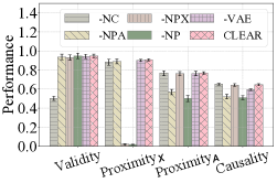
(a) Community

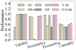
(b) Ogbg-molhiv

Figure 4: Ablation studies.

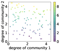
(a) Original data

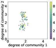
(b) CFEs from CLEAR-VAE

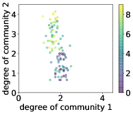
(c) CFEs from CLEAR

Figure 5: Explainability through CFEs on Community.

To evaluate the effectiveness of different components in CLEAR, we conduct ablation study with the following variants: 1) CLEAR-NC. In this variant, we remove the counterfactual prediction loss; 2) CLEAR-NPA, we remove the similarity loss w.r.t. graph structure; 3) CLEAR-NPX, we remove the similarity loss w.r.t. node features; 4) CLEAR-NP, we remove all the similarity loss; 5) CLEAR-VAE, the backbone of our framework. As shown in Fig. 4, we have the following observations: 1) The validity of CLEAR-NC degrades dramatically due to the lack of counterfactual prediction loss; 2) The performance w.r.t. proximity is worse in CLEAR-NPA, CLEAR-NPX, and CLEAR-NP as the similarity loss is removed. Besides, removing the similarity loss can also hurt the performance of causality when the variables in the causal relation of interest $R$ are involved. For example, in Community, CLEAR-NPA performs much worse in causality (as $R$ in Community involves node degree in graph structure), while in Ogbg-molhiv, the performance in causality of CLEAR-NPX is eroded (as $R$ on Ogbg-molhiv involves node features); 3) The performance w.r.t. causality is impeded in CLEAR-VAE. This observation validates the effectiveness of the auxiliary variable for promoting causality. Similar observations can also be found in the ablation study on the IMDB-M dataset, which is shown in Appendix C.

4.7 RQ3: Explainability through CFEs

To investigate how CFE on graphs promote model explainability, we take a closer look in the generated counterfactuals. Due to the space limit, we only show our investigation on the Community dataset. Fig. 5(a) shows the distribution of two variables: the average node degree in the first community and in the second community in the original dataset, i.e., $\text{deg}_{1}(A)$ and $\text{deg}_{2}(A)$. Fig. 5(b) shows the distribution of these two variables in counterfactuals generated by CLEAR-VAE. We observe that these counterfactuals are distributed close to the decision boundary, i.e., $\text{deg}_{1}(A)=\text{ADG}_{1}$, where $\text{ADG}_{1}$ is a constant around 2. This is because that the counterfactuals are enforced to change their predicted labels with perturbation as slight as possible. Fig. 5(c) shows the distribution of these two variables $\text{deg}_{1}(A)$ and $\text{deg}_{2}(A)$ in counterfactuals generated by CLEAR. Different colors denote different values of the auxiliary variable $S$. Notice that based on the causal model (in Appendix B), the exogenous variables are distributed in a narrow range when the value of $S$ is fixed, thus the same color also indicates similar values of exogenous variables. We observe that compared with the color distribution in Fig. 5(b), the color distribution in Fig. 5(c) is more consistent with Fig. 5(a). This indicates that compared with CLEAR-VAE, CLEAR can better capture the values of exogenous variables, and thus the counterfactuals generated by CLEAR are more consistent with the underlying causal model. To better illustrate the explainability provided by CFE, we further conduct case studies to compare the original graphs and their counterfactuals in Appendix C.

4.8 RQ4: Parameter Study

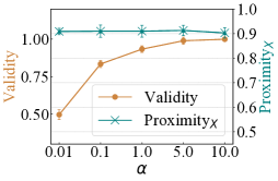
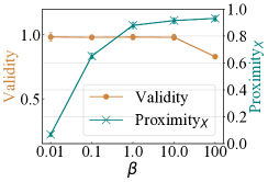
Figure 6: Parameter studies on Ogbg-molhiv.

To evaluate the robustness of our method, we test the model performance under different settings of hyperparameters. We vary $\alpha\in\{0.01,0.1,1.0,5.0,10.0\}$ and $\beta\in\{0.01,0.1,1.0,10.0,100\}$. Due to the space limit, we only show the parameter study on Ogbg-molhiv, but similar observations can be found in other datasets. As shown in Fig. 6, the selection of $\alpha$ and $\beta$ controls the tradeoff between different goals in the objective function. But generally speaking, the proposed framework is not very sensitive to the hyparameter setting. More studies regarding other parameters are in Appendix C.

5 Related Work

Counterfactual explanations on tabular data. Counterfactual explanations have attracted increasing attentions wachter2017counterfactual ; verma2020counterfactual ; mishra2021survey ; tolomei2017interpretable . Especially, recent works also consider more aspects in CFEs, such as actionability ustun2019actionable ; poyiadzi2020face , sparsity guidotti2018local ; mothilal2020explaining ; dandl2020multi , data manifold closeness dhurandhar2018explanations ; dhurandhar2019model , diversity mothilal2020explaining ; russell2019efficient , feasibility mahajan2019preserving ; poyiadzi2020face , causality mahajan2019preserving ; karimi2020algorithmic ; karimi2021algorithmic , and amortized inference mahajan2019preserving . These methods include model-agnostic poyiadzi2020face ; dandl2020multi ; dhurandhar2019model methods and model-accessible wachter2017counterfactual ; tolomei2017interpretable methods. Recently, a few studies mahajan2019preserving ; bajaj2021robust develop generative CFE generators based on variational autoencoder. However, most of current CFE approaches only focus on tabular or image datasets, and can not be directly grafted for the graph data.

Counterfactual explanations on graphs. There have been a few studies related to CFEs on graphs numeroso2021meg ; lucic2021cf ; bajaj2021robust ; abrate2021counterfactual ; ying2019gnnexplainer ; yuan2020explainability . Among them, GNNExplainer ying2019gnnexplainer identifies subgraphs which are important for graph neural network (GNN) model prediction kipf2016semi ; velivckovic2017graph ; kipf2016variational ; jiao2020sub ; wang2018graphgan ; fey2019fast ; hamilton2020graph . It can be adapted to generate counterfactuals by perturbing the identified important subgraphs. Similarly, RCExplainer bajaj2021robust generates CFEs by removing important edges from the original graph, but it is based on an assumption that GNN prediction model is partially accessible. CF-GNNExplainer lucic2021cf studies counterfactual explanations for GNN models in node classification tasks. Besides, a few domain-specific methods numeroso2021meg ; abrate2021counterfactual are particularly designed for certain domains such as chemistry and brain diagnosis. However, all the above methods are either limited in a specific setting (e.g., the prediction model is accessible), or heavily based on domain knowledge. Many general and important issues in model-agnostic CFE generation on graphs still lack exploration.

Graph generative models. Many efforts simonovsky2018graphvae ; you2018graphrnn ; grover2019graphite ; ding2022data have been made in graph generative models recently. Among them, GraphVAE simonovsky2018graphvae develops a VAE-based mechanism to generate graphs from continuous embeddings. GraphRNN you2018graphrnn is an autoregressive generative model for graphs. It generates graphs by decomposing the graph generation process into a sequence of node and edge formations. Furthermore, a surge of domain-specific graph generative models de2018molgan ; jin2018junction ; preuer2018frechet are developed with domain knowledge incorporated. Although different from CFE methods in their goals, graph generative models can serve as the cornerstone of our work for CFE generation on graphs. Our framework can be compatible with techniques in different graph generative models.

6 Conclusion

In this paper, we study an important problem of counterfactual explanations on graphs. More specifically, we aim to facilitate the optimization, generalization, and causality in CFE generation on graphs. To address this problem, we propose a novel framework CLEAR, which uses a graph variational autoencoder mechanism to enable efficient optimization in graph data, and generalization to unseen graphs. Furthermore, we promote the causality in counterfactuals by improving the model identifiability with the help of an auxiliary observed variable. Extensive experiments are conducted to validate the superiority of the proposed framework in different aspects. In the future, more properties of the counterfactuals in graphs, such as diversity, data manifold closeness can be considered. Besides, incorporating different amount and types of prior knowledge regarding the causal models into CFE generation on graphs is also an interesting direction.

Checklist

1. For all authors…

   1. Do the main claims made in the abstract and introduction accurately reflect the paper’s contributions and scope?[Yes]

   2. Did you describe the limitations of your work? [Yes] See Appendix D.

   3. Did you discuss any potential negative societal impacts of your work? [Yes] See Appendix D.

   4. Have you read the ethics review guidelines and ensured that your paper conforms to them?[Yes]

2. If you are including theoretical results…

   1. Did you state the full set of assumptions of all theoretical results? [Yes] See Section 3.2 and Appendix A.

   2. Did you include complete proofs of all theoretical results? [Yes] See Appendix A.

3. If you ran experiments…

   1. Did you include the code, data, and instructions needed to reproduce the main experimental results (either in the supplemental material or as a URL)? [Yes] In the submitted supplementary materials.

   2. Did you specify all the training details (e.g., data splits, hyperparameters, how they were chosen)? [Yes] See Section 4, Appendix B and C.

   3. Did you report error bars (e.g., with respect to the random seed after running experiments multiple times)? [Yes] All the experimental results are provided with error bars.

   4. Did you include the total amount of compute and the type of resources used (e.g., type of GPUs, internal cluster, or cloud provider)? [Yes] See Appendix B.

4. If you are using existing assets (e.g., code, data, models) or curating/releasing new assets…

   1. If your work uses existing assets, did you cite the creators? [Yes] See Appendix B.

   2. Did you mention the license of the assets? [Yes] See Appendix B.

   3. Did you include any new assets either in the supplemental material or as a URL? [Yes] The source code of our proposed framework is included in the supplemental material. It will be released after publication.

   4. Did you discuss whether and how consent was obtained from people whose data you’re using/curating? [N/A] The creators developed the adopted datasets based on either publicly available data or data with proper consent.

   5. Did you discuss whether the data you are using/curating contains personally identifiable information or offensive content? [N/A] We use well-known public datasets in this paper, and they do not contain personally identifiable information or offensive content.

5. If you used crowdsourcing or conducted research with human subjects…

   1. Did you include the full text of instructions given to participants and screenshots, if applicable? [N/A]

   2. Did you describe any potential participant risks, with links to Institutional Review Board (IRB) approvals, if applicable? [N/A]

   3. Did you include the estimated hourly wage paid to participants and the total amount spent on participant compensation? [N/A]

Appendix A Theory

Theorem 1. The evidence lower bound (ELBO) to optimize the framework is:

$$\begin{split}\ln P(G^{CF}|S,Y^{*},G)\geq\mathbb{E}_{Q}[\ln P(G^{CF}|Z,S,Y^{*},G)]-\text{KL}(Q(Z|G,S,Y^{*})\|P(Z|G,S,Y^{*})),\end{split}$$ (8)

Proof.

$$\begin{split}&\ln P(G^{CF}|S,Y^{*},G)\\ =&\,\ln\int_{Z}P(G^{CF},Z|S,Y^{*},G)dZ\\ =&\,\ln\int_{Z}Q(Z|G,S,Y^{*})\frac{P(G^{CF},Z|S,Y^{*},G)}{Q(Z|G,S,Y^{*})}dZ\\ \geq&\int_{Z}Q(Z|G,S,Y^{*})\ln\frac{P(G^{CF},Z|S,Y^{*},G)}{Q(Z|G,S,Y^{*})}dZ\\ =&\,\mathbb{E}_{Q}[\ln\frac{P(G^{CF},Z|S,Y^{*},G)}{Q(Z|G,S,Y^{*})}]\\ =&\,\mathbb{E}_{Q}[\ln\frac{P(G^{CF}|Z,S,Y^{*},G)\cdot P(Z|G,S,Y^{*})}{Q(Z|G,S,Y^{*})}]\\ =&\,\mathbb{E}_{Q}[\ln{P(G^{CF}|Z,S,Y^{*},G)}]-\mathbb{E}_{Q}[\ln\frac{Q(Z|G,S,Y^{*})}{P(Z|G,S,Y^{*})}]\\ =&\,\mathbb{E}_{Q}[\ln P(G^{CF}|Z,S,Y^{*},G)]-\text{KL}(Q(Z|G,S,Y^{*})\|P(Z|G,S,Y^{*})).\end{split}$$ (9)

∎

Appendix B Reproducibility

In this section, we provide more details of model implementation and experiment setup for reproducibility of the experimental results.

B.1 Details of Model Implementation

B.1.1 Details of the Prediction Model

The prediction model $f$ is implemented with a graph neural network based model. Specifically, this prediction model includes the following components:

• Three layers of graph convolutional network (GCN) [34] with learnable node masks.

• Two graph pooling layers with mean pooling and max pooling, respectively.

• A two-layer multilayer perceptron (MLP) with batch normalization and ReLU activation function.

The prediction model uses negative log likelihood loss. The representation dimension is set as $32$. We use Adam optimizer, set the learning rate as $0.001$, weight decay as $1e\!-\!5$, the training epochs as $600$, dropout rate as $0.1$, and batch size as $500$. As shown in Table 2, we observe that the prediction model $f$ achieves high performance of graph classification on all datasets.

Table 2: Performance of the prediction model on the test data of the three datasets.

Dataset	Community	Ogbg-molhiv	IMDB-M
Accuracy	$0.949\pm 0.006$	$0.897\pm 0.004$	$0.995\pm 0.002$
AUC-ROC	$0.993\pm 0.002$	$0.997\pm 0.002$	$1.000\pm 0.001$
F1-score	$0.947\pm 0.005$	$0.906\pm 0.004$	$0.994\pm 0.003$

B.1.2 Details of CLEAR

CLEAR is designed in a general way, which can be adaptable to different graph representation learning modules and different techniques in graph generative models. Specifically, in our implementation, we apply a graph convolution [34] based module as the encoder, and use a multilayer perceptron (MLP) as the decoder. We also use MLPs to learn the mean and covariance of the prior distribution of the latent variables. We choose the pairwise distance using $L_{2}$ norm to implement $d_{X}(\cdot)$, and use cross entropy loss to implement $d_{A}(\cdot)$. We implement the counterfactual prediction loss with the negative log likelihood loss. Following [16], we assume that the maximum number of nodes in the graph is $k$, and use a graph matching technique to align the input graph and counterfactuals. The detailed implementation contains the following components:

• Prior distribution: Two different two-layer MLPs are used to learn the mean and covariance of the prior distribution $P(Z|G,S,Y^{*})$, respectively.

• Encoder: The encoder contains a single-layer graph convolutional network, a graph pooling layer with mean pooling, and two linear layers with batch normalization and ReLU activation function to learn the mean and covariance of the approximate posterior distribution $Q(Z|G,S,Y^{*})$.

• Decoder: The decoder uses two three-layer MLPs to output the node features and graph structure of the counterfactual $G^{CF}$, respectively. These MLPs use batch normalization, and take ReLU as activation function in the middle layers. At the last layer of decoder, the MLP which generates the graph structure uses Sigmoid as activation function to output a probabilistic adjancency matrix $\hat{A}^{CF}$ with elements in range $[0,1]$.

Inspired by [16], we use a graph matching technique to align the input graph and counterfactuals. Specifically, we learn a graph matching matrix $M=\{0,1\}^{k\times n}$ to match the generated counterfactual with the original explainee graph. Here, $n$ is the number of nodes in the original graph, and $M_{(i,j)}=1$ if and only if node $i$ is in $G^{CF}$ and node $j$ is in $G$, and $M_{(i,j)}=0$ otherwise.

B.2 Details of Experiment Setup

B.2.1 Baseline Settings

Here we introduce more details of baseline setting:

• Random: For each explainee graph, it randomly perturbs the graph structure for at most $T=150$ steps. In each step, at most one edge can be inserted or removed. We stop the process if the perturbed graph can achieve a desired predicted label.

• GNNExplainer: For each graph, GNNExplainer [12] outputs an edge mask which estimates the importance of different edges in model prediction. In CFE generation, we set a threshold $0.5$ and remove edges with edge mask weight smaller than the threshold. Although GNNExplainer can also identify important node features in a similar way, when we apply GNNExplainer for CFE generation, the perturbation on node features cannot be designed as straightforwardly as the perturbation on graph structure, thus we did not involve perturbation on node features in GNNExplainer.

• CF-GNNExplainer: CF-GNNExplainer [9] is originally proposed for node classification tasks, and it only focuses on the perturbations on the graph structure. Originally, for each explainee node, it takes its neighborhood subgraph as input. To apply it on graph classification tasks, we use the graph instance as the neighborhood subgraph, and assign the graph label as the label for all nodes in the graph. We set the number of iterations to generate counterfactuals for each graph as $150$.

• MEG: MEG [6] is specifically proposed for molecular prediction tasks. This model explicitly incorporates domain knowledge in chemistry. The CFE generator is developed based on reinforcement learning, and it designs the reward based on the prediction on the counterfactual, as well as the similarity between the original graph and the counterfactual. In each step, MEG enumerates all possible perturbations (e.g., adding an atom) which are valid w.r.t. chemistry rules to form an action set. We apply it to general graphs by removing the constraints of domain knowledge, and enumerating the perturbations as: 1) adding or removing a node; 2) adding or removing an edge; 3) staying the same. We set the number of action steps as $150$.

B.2.2 Datasets

Table 3: Detailed statistics of the datasets.

Dataset	Community	Ogbg-molhiv	IMDB-M
# of graphs	$10,000$	$31,957$	$1,160$
Avg # of nodes	$20$	$20.8$	$9.4$
Avg # of edges	$45.0$	$22.4$	$32.8$
Max # of nodes	$20$	$30$	$15$
# of classes	$2$	$2$	$2$
Feature dimension	$16$	$11$	$2$
Avg node degree	$2.24$	$1.07$	$3.4$

For each dataset, we filter out the graphs with the number of nodes larger than a threshold $k$. The setting of $k$ (i.e., max # of nodes) can be found in Table 3. As some of the baselines need to be optimized separately for each graph, we compare the performance of all methods on a small set of test data with $20$ graphs for evaluation in RQ1. For other RQs, we evaluate our framework on the whole test data.

1. Community. We first generate a synthetic dataset in which we can fully control the data generation process. In this dataset, each graph consists of two $10$-node communities generated using the Erdös-Rényi (E-R) model [24] with edge rate $p_{1}$ and $p_{2}$, respectively. Specifically, we simulate the data with the following causal model:

$$S\sim\text{Uniform}(\{0,...,9\}),\,\,p_{1}=U_{1}\sim\text{Uniform}([0,1]),$$

$$U_{2}\!\sim\!\text{Uniform}([\delta S+b,\delta(S+1)+b]),\,p_{2}\!=\!\max\{0,\min\{1,-0.15p_{1}+U_{2}\}\!\},$$

$$X\sim\mathcal{N}(0,I),\,\,Y\sim\text{Bernoulli}(\text{Sigmoid}(\text{deg}_{1}(A)-\text{ADG}_{1}+\epsilon_{y})).$$ (10)

$U_{1}$ and $U_{2}$ are two exogenous variables associated with $p_{1}$ and $p_{2}$, respectively. Notice that $p_{2}$ is determined by $p_{1}$ and $U_{2}$. Here, the auxiliary variable $S$ provides help to infer the value of exogenous variables (specifically, $U_{2}$ in this case). We set $\delta=0.085,b=0.15$. $p_{1}$ and $p_{2}$ thereby generate the graph structure inside the two communities, respectively. We also randomly add few edges between these two communities. The edges connecting two communties are randomly generated with an edge rate of $0.05$. In this way, the adjacency matrix $A$ of each graph is simulated. $\text{deg}_{1}(A)$ (determined by $p_{1}$) denotes the average node degree in the first community of each graph $A$. Label generation: The label $Y$ is determined by $\text{deg}_{1}(A)$ together with a Gaussian noise $\epsilon_{y}\sim\mathcal{N}(0,0.01^{2})$. $\text{ADG}_{1}$ is a constant, which is the average value of $\text{deg}_{1}(A)$ over all graphs. Causality: To elicit a different predicted label, $\text{deg}_{1}(A)$ in the counterfactual is supposed to be perturbed, while other variables can remain the same. But considering that with the above causal model, when $\text{deg}_{1}(A)$ increases (decreases), the average node degree in the second community $\text{deg}_{2}(A)$ (determined by $p_{2}$) should decrease (increase) correspondingly. We take this causal relation $\text{deg}_{1}(A)\rightarrow\text{deg}_{2}(A)$ as our causal relation of interest, and denote it as $R$. Correspondingly, we define a causal constraint for evaluation of causality: “$(\text{deg}_{1}(A^{CF})>\text{deg}_{1}(A))\Rightarrow(\text{deg}_{2}(A^{CF})<\text{deg}_{2}(A))"$ OR “$(\text{deg}_{1}(A^{CF})<\text{deg}_{1}(A))\Rightarrow(\text{deg}_{2}(A^{CF})>\text{deg}_{2}(A))"$.

2. Ogbg-molhiv. Ogbg-molhiv is adopted from the MoleculeNet [47] datasets. All molecules are preprocessed with RDKit [48]. The original node features are 9-dimensional, containing atom features such as atomic number, formal charge and chirality. In this dataset, each graph stands for a molecule, where each node represents an atom, and each edge is a chemical bond. As the ground-truth causal model is unavailable, we simulate the label and causal relation of interest as follows: Label generation: $Y\sim\text{Bernoulli}(\text{Sigmoid}(X_{1}-\text{AVG}_{x1}))$, where $X_{1}$ is the average value of a synthetic node feature over all nodes in each graph. This node feature is generated for each node from distribution $\text{Uniform}(0,1)$. $\text{AVG}_{x1}$ means the average value of $X_{1}$ over all graphs. Causality: We also add a causal relation of interest $R$ between $X_{1}$ and another synthetic node feature $X_{2}$: $X_{2}=U_{2}+0.5X_{1}$. Here $U_{2}$ is simulated in a similar way as the Community dataset. Correspondingly, we have the following causal constraint: “$(X_{1}^{CF}>X_{1})\Rightarrow(X_{2}^{CF}>X_{2})"$ OR “$(X_{1}^{CF}<X_{1})\Rightarrow(X_{2}^{CF}<X_{2})"$.

3. IMDB-M. This dataset contains movie collaboration networks from IMDB. In each graph, each node represents an actor or an actress, and each edge represents the collaboration between two actors or actresses in the same movie. Similarly as the above datasets, we simulate the label and causal relation of interest as follows: Label generation: $Y\sim\text{Bernoulli}(\text{Sigmoid}(\text{deg}(A)-\text{ADG}+\epsilon_{y})$. $\text{deg}(A)$ is the average node degree in graph with adjacency matrix $A$. ADG is the average value of $\text{deg}(A)$ over all graphs. Causality: We also add a causal relation of interest $R$ from the average node degree to a synthetic node feature: $X_{1}=U_{1}+0.5\text{deg}(A)/\text{ADG}$, where $U_{1}\sim\text{Uniform}[0.1S,0.1S+0.1]$, $S\sim\text{Uniform}\{0,...,9\}$. We denote the causal relation $\text{deg}(A)\rightarrow X_{1}$ as $R$, and define an associated causal constraint: “$(\text{deg}(A^{CF})>\text{deg}(A))\Rightarrow(X_{1}^{CF}>X_{1})"$ OR “$(\text{deg}(A^{CF})<\text{deg}_{1}(A))\Rightarrow(X_{1}^{CF}<X_{1})"$.

B.2.3 Experiment Settings

All the experiments are conducted in the following environment:

• Python 3.6

• Pytorch 1.10.1

• Pytorch-geometric 1.7.0

• Scikit-learn 1.0.1

• Scipy 1.6.2

• Networkx 2.5.1

• Numpy 1.19.2

• Cuda 10.1

In all the experiments of counterfactual explanation, each dataset is randomly split into 60%/20%/20% training/validation/test set. Unless otherwise specified, we set the hyperparameters as $\alpha=5.0$ and $\beta=10.0$. The batch size is $500$, and the representation dimension is $32$. The graph prediction models trained on all the above datasets perform well in label prediction (AUC-ROC score over 95% and F1 score over 90% on test data). We use NetworkX [49] to generate synthetic graphs. In our CFE generator CLEAR, the learning rate is 0.001, the number of epochs is 1,000. All the experimental results are averaged over ten repeated executions. The implementation is based on Pytorch. We use the Adam optimizer for model optimization.

Appendix C More Experimental Results

C.1 Ablation Study

Fig. 8 shows the results of ablation studies on the IMDB-M dataset. The observations are generally consistent with the observations on other two datasets as described in Section 4.6.

C.2 Case Study

To better illustrate the explainability provided by CFE, we further conduct case studies to compare the original graphs and their counterfactuals. In the Community dataset, Fig. 8 shows the change from original graphs to their counterfactuals w.r.t. the average node degree in the first community and in the second community, i.e., $\text{deg}_{1}(A)$ and $\text{deg}_{2}(A)$. Here, Fig. 8 has the same x-axis and y-axis as Fig. 5. In Fig. 8, we randomly select $6$ graphs and show them in different shapes of markers. The colors denote their values of $S$ with the same colorbar in Fig. 5(a-c). In Fig. 8, we connect the pairs (original, counterfactual generated by CLEAR) with solid lines, and connect the pairs (original, counterfactual generated by CLEAR-VAE) with dashed lines. We have the following observations: 1) Compared with the input graph, the counterfactuals generated by CLEAR-VAE and CLEAR both make the correct perturbations to achieve the desired label (moving the variable $\text{deg}_{1}(A)$ across the decision boundary at around $\text{deg}_{1}(A)=2$); 2) The counterfactuals generated by CLEAR better match the causality than CLEAR-VAE in two aspects: a) Qualitatively, the counterfactuals generated by CLEAR better satisfy the causal constraints introduced in the dataset description, i.e., $\text{deg}_{2}(A)$ increases (decreases) when $\text{deg}_{1}(A)$ decreases (increases); 2) Quantitatively, the changes from original graphs to their counterfactuals fit in well with the associated structural equations $(\text{deg}_{1}(A),U_{2})\rightarrow\text{deg}_{2}(A)$. Notice that in counterfactuals, $\text{deg}_{1}(A)$ changes but $U_{2}$ is supposed to maintain its original value.

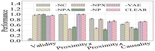
Figure 7: Ablation studies on the IMDB-M dataset.

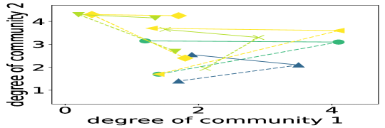
Figure 8: Case study.

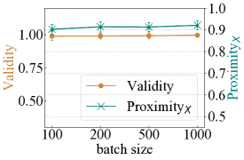
(a) Batch size

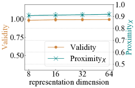
(b) Representation dimension

Figure 9: Parameter studies on Ogbg-molhiv regarding batch size and representation dimension.

C.3 Parameter Study

Here, we conduct further parameter study with respect to the batch size and representation dimension. Specifically, we vary the batch size from range $\{100,500,1000,2000\}$, and the representation dimension from range $\{8,16,32,64\}$. From the results shown in Fig. 9, we observe that the performance of CLEAR under different settings of these parameters is generally stable. This observation further validates the robustness of our framework.

Appendix D Further Discussion

CFEs in Other Tasks on Graphs. In this paper, we mainly focus on the task of graph classification, but it is worth noting that the proposed framework CLEAR can also be used for counterfactual explanations in other tasks such as node classification. More specifically, in a node classification task, CLEAR can generate CFEs for nodes with the same loss function in Eq. (5). But differently, the encoder here learns node representations instead of graph representations at the bottleneck layer. Besides, in this case, $Y^{*}$ is a vector which contains the desired labels for all the training nodes on graph $G$, and $S$ is the vector of auxiliary variables for all the training nodes. Notice that in a graph, nodes are often not independent. To obtain a valid counterfactual for an explainee node, not only can we change the explainee node’s own features and adjacent edges, but we can also change other nodes’ features or any other part of the graph structure. Therefore, the decoder still needs to generate a graph $G^{CF}$ as a counterfactual (but this process can be more efficient, as in many scenarios, we only need to generate counterfactuals for each node’s neighboring subgraph instead of the whole graph). Similarly, our framework can also be extended to generate CFEs for graphs in other tasks, such as link prediction.

Limitation, Future Work, and Negative Societal Impacts. In this work, we mainly focus on promoting optimization, generalization, and causality in counterfactual explanations on graphs, while other important targets (e.g., actionability [26], sparsity [28], diversity [29], and data manifold closeness [31]) in traditional counterfactual explanations could be considered in graph data in the future. Noticeably, the definition and evaluation metrics with respect to these targets should be specifically tailored for graphs, rather than directly employed in the same way as other types of data. Besides, in terms of causality, another interesting direction is incorporating different levels of prior knowledge and assumptions regarding the underlying causal model into CFE generation on graphs, and quantifying the influence of different levels of prior knowledge and assumptions on the CFE performance. Currently, we have not found any negative societal impact regarding this work.

References

- [1] Pantelis Linardatos, Vasilis Papastefanopoulos, and Sotiris Kotsiantis. Explainable ai: a review of machine learning interpretability methods. Entropy, 2020.
- [2] Sandra Wachter, Brent Mittelstadt, and Chris Russell. Counterfactual explanations without opening the black box: Automated decisions and the gdpr. Harv. JL & Tech., 2017.
- [3] Sahil Verma, John Dickerson, and Keegan Hines. Counterfactual explanations for machine learning: A review. arXiv preprint, 2020.
- [4] Divyat Mahajan, Chenhao Tan, and Amit Sharma. Preserving causal constraints in counterfactual explanations for machine learning classifiers. arXiv preprint, 2019.
- [5] Saumitra Mishra, Sanghamitra Dutta, Jason Long, and Daniele Magazzeni. A survey on the robustness of feature importance and counterfactual explanations. arXiv preprint, 2021.
- [6] Danilo Numeroso and Davide Bacciu. Meg: Generating molecular counterfactual explanations for deep graph networks. arXiv preprint, 2021.
- [7] Hans-Georg Wolff and Klaus Moser. Effects of networking on career success: a longitudinal study. Journal of applied psychology, 94(1):196, 2009.
- [8] Predict grant applications. https://www.kaggle.com/c/unimelb.
- [9] Ana Lucic, Maartje ter Hoeve, Gabriele Tolomei, Maarten de Rijke, and Fabrizio Silvestri. Cf-gnnexplainer: Counterfactual explanations for graph neural networks. arXiv preprint, 2021.
- [10] Mohit Bajaj, Lingyang Chu, Zi Yu Xue, Jian Pei, Lanjun Wang, Peter Cho-Ho Lam, and Yong Zhang. Robust counterfactual explanations on graph neural networks. NeurIPS, 2021.
- [11] Carlo Abrate and Francesco Bonchi. Counterfactual graphs for explainable classification of brain networks. arXiv preprint, 2021.
- [12] Rex Ying, Dylan Bourgeois, Jiaxuan You, Marinka Zitnik, and Jure Leskovec. Gnnexplainer: Generating explanations for graph neural networks. NeurIPS, 2019.
- [13] Hao Yuan, Haiyang Yu, Shurui Gui, and Shuiwang Ji. Explainability in graph neural networks: A taxonomic survey. arXiv preprint, 2020.
- [14] Ilyes Khemakhem, Diederik Kingma, Ricardo Monti, and Aapo Hyvarinen. Variational autoencoders and nonlinear ica: A unifying framework. In AISTATS, 2020.
- [15] Judea Pearl. Causality. 2009.
- [16] Martin Simonovsky and Nikos Komodakis. Graphvae: Towards generation of small graphs using variational autoencoders. In ICANN, 2018.
- [17] Diederik P Kingma and Max Welling. Auto-encoding variational bayes. arXiv preprint, 2013.
- [18] Martin Pawelczyk, Klaus Broelemann, and Gjergji Kasneci. Learning model-agnostic counterfactual explanations for tabular data. In WWW, 2020.
- [19] Amir-Hossein Karimi, Julius Von Kügelgen, Bernhard Schölkopf, and Isabel Valera. Algorithmic recourse under imperfect causal knowledge: a probabilistic approach. arXiv preprint, 2020.
- [20] Amir-Hossein Karimi, Bernhard Schölkopf, and Isabel Valera. Algorithmic recourse: from counterfactual explanations to interventions. In ACM FAccT, 2021.
- [21] Aapo Hyvarinen, Hiroaki Sasaki, and Richard Turner. Nonlinear ica using auxiliary variables and generalized contrastive learning. In AISTATS, 2019.
- [22] Shohei Shimizu, Patrik O Hoyer, Aapo Hyvärinen, Antti Kerminen, and Michael Jordan. A linear non-gaussian acyclic model for causal discovery. Journal of Machine Learning Research, 2006.
- [23] Ricardo Pio Monti, Kun Zhang, and Aapo Hyvärinen. Causal discovery with general non-linear relationships using non-linear ica. In Uncertainty in Artificial Intelligence, 2020.
- [24] P Erdős and A Rényi. On random graphs i. publicationes mathematicae (debrecen). 1959.
- [25] Gabriele Tolomei, Fabrizio Silvestri, Andrew Haines, and Mounia Lalmas. Interpretable predictions of tree-based ensembles via actionable feature tweaking. In SIGKDD, 2017.
- [26] Berk Ustun, Alexander Spangher, and Yang Liu. Actionable recourse in linear classification. In ACM FAccT, 2019.
- [27] Rafael Poyiadzi, Kacper Sokol, Raul Santos-Rodriguez, Tijl De Bie, and Peter Flach. Face: Feasible and actionable counterfactual explanations. In AIES, 2020.
- [28] Riccardo Guidotti, Anna Monreale, Salvatore Ruggieri, Dino Pedreschi, Franco Turini, and Fosca Giannotti. Local rule-based explanations of black box decision systems. arXiv preprint, 2018.
- [29] Ramaravind K Mothilal, Amit Sharma, and Chenhao Tan. Explaining machine learning classifiers through diverse counterfactual explanations. In ACM FAccT, 2020.
- [30] Susanne Dandl, Christoph Molnar, Martin Binder, and Bernd Bischl. Multi-objective counterfactual explanations. In PPSN, 2020.
- [31] Amit Dhurandhar, Pin-Yu Chen, Ronny Luss, Chun-Chen Tu, Paishun Ting, Karthikeyan Shanmugam, and Payel Das. Explanations based on the missing: Towards contrastive explanations with pertinent negatives. arXiv preprint, 2018.
- [32] Amit Dhurandhar, Tejaswini Pedapati, Avinash Balakrishnan, Pin-Yu Chen, Karthikeyan Shanmugam, and Ruchir Puri. Model agnostic contrastive explanations for structured data. arXiv preprint, 2019.
- [33] Chris Russell. Efficient search for diverse coherent explanations. In ACM FAccT, 2019.
- [34] Thomas N Kipf and Max Welling. Semi-supervised classification with graph convolutional networks. ICLR, 2017.
- [35] Petar Veličković, Guillem Cucurull, Arantxa Casanova, Adriana Romero, Pietro Lio, and Yoshua Bengio. Graph attention networks. ICLR, 2018.
- [36] Thomas N Kipf and Max Welling. Variational graph auto-encoders. NeurIPS Workshop on Bayesian Deep Learning, 2016.
- [37] Yizhu Jiao, Yun Xiong, Jiawei Zhang, Yao Zhang, Tianqi Zhang, and Yangyong Zhu. Sub-graph contrast for scalable self-supervised graph representation learning. In IEEE ICDM, 2020.
- [38] Hongwei Wang, Jia Wang, Jialin Wang, Miao Zhao, Weinan Zhang, Fuzheng Zhang, Xing Xie, and Minyi Guo. Graphgan: Graph representation learning with generative adversarial nets. In AAAI, 2018.
- [39] Matthias Fey and Jan Eric Lenssen. Fast graph representation learning with pytorch geometric. ICLR Workshop on Representation Learning on Graphs and Manifolds, 2019.
- [40] William L Hamilton. Graph representation learning. Synthesis Lectures on Artifical Intelligence and Machine Learning, 2020.
- [41] Jiaxuan You, Rex Ying, Xiang Ren, William Hamilton, and Jure Leskovec. Graphrnn: Generating realistic graphs with deep auto-regressive models. In ICML, 2018.
- [42] Aditya Grover, Aaron Zweig, and Stefano Ermon. Graphite: Iterative generative modeling of graphs. In ICML, 2019.
- [43] Kaize Ding, Zhe Xu, Hanghang Tong, and Huan Liu. Data augmentation for deep graph learning: A survey. arXiv preprint, 2022.
- [44] Nicola De Cao and Thomas Kipf. Molgan: An implicit generative model for small molecular graphs. arXiv preprint, 2018.
- [45] Wengong Jin, Regina Barzilay, and Tommi Jaakkola. Junction tree variational autoencoder for molecular graph generation. In ICML, 2018.
- [46] Kristina Preuer, Philipp Renz, Thomas Unterthiner, Sepp Hochreiter, and Gunter Klambauer. Fréchet chemnet distance: a metric for generative models for molecules in drug discovery. Journal of chemical information and modeling, 2018.
- [47] Zhenqin Wu, Bharath Ramsundar, Evan N Feinberg, Joseph Gomes, Caleb Geniesse, Aneesh S Pappu, Karl Leswing, and Vijay Pande. Moleculenet: a benchmark for molecular machine learning. Chemical science, 2018.
- [48] Greg Landrum et al. Rdkit: Open-source cheminformatics. 2006.
- [49] Aric Hagberg, Pieter Swart, and Daniel S Chult. Exploring network structure, dynamics, and function using networkx. Technical report, Los Alamos National Lab.(LANL), Los Alamos, NM (United States), 2008.