ALMA Observation of a $z\gtrsim 10$ Galaxy Candidate Discovered with JWST

Abstract

We report the ALMA observation of a $z\gtrsim 10$ galaxy candidate (GHZ1) discovered from the GLASS-JWST Early Release Science Program. Our ALMA program aims to detect the [$\textrm{O}\scriptstyle\mathrm{III}$] emission line at the rest-frame 3393.0062 GHz ($88.36\mu$m) and far-IR continuum emission with the spectral window setup seamlessly covering a 26.125 GHz frequency range ($10.10<z<11.14$). A total of 7 hours of on-source integration was employed, using four frequency settings to cover the full range (1.7 hours per setting), with $0\arcsec.7$ angular resolution. No line or continuum is clearly detected, with a 5$\sigma$ upper limit of the line emission of 0.93 mJy beam^-1 at 25 km s^-1 channel^-1 and of the continuum emission of 30$\mu$Jy beam^-1. We report marginal spectral (at 225 km s^-1 resolution) and continuum features ($4.1\sigma$ and $2.6\sigma$ peak signal-to-noise ratio, respectively), within $0\arcsec.17$ from the JWST position of GHZ1. This spectral feature implies $z=10.38$ and needs to be verified with further observations. Assuming that the best photometric redshift estimate ($z=10.60^{+0.52}_{-0.60}$) is correct, the broadband galaxy spectral energy distribution model for the $3\sigma$ upper limit of the continuum flux from GHZ1 suggests that GHZ1 has a small amount of dust ($M_{d}\lesssim 10^{4}M_{\odot}$) with high temperature ($T_{d}\gtrsim 90$K). The $5\sigma$ upper limit of the [$\textrm{O}\scriptstyle\mathrm{III}$]_88μm line luminosity and the inferred star formation rate of GHZ1 is consistent with the properties of the low metallicity dwarf galaxies. We also report serendipitous clear detections of six continuum sources at the locations of the JWST galaxy counterparts in the field.

1 Introduction

With the recent commissioning and the operation of JWST, the galaxy formation study enters into a new era: the JWST early release science (ERS) programs are discovering many galaxy candidates at $z\gtrsim 10$ (e.g., Adams et al., 2023; Atek et al., 2023; Castellano et al., 2022a; Finkelstein et al., 2022; Labbe et al., 2022; Donnan et al., 2023; Harikane et al., 2023; Naidu et al., 2022a; Whitler et al., 2023; Yan et al., 2023). Although the majority of them is not spectroscopically confirmed yet, the rate of discovery has been prodigious and has opened up a new uncharted territory.

The unexpectedly large number of $z\gtrsim 10$ galaxy candidates reported recently has already started to challenge current galaxy formation models (Boylan-Kolchin, 2022; Ferrara et al., 2022; Mason et al., 2023) and the cosmology (Lovell et al., 2023; Menci et al., 2022). The next key observational step is to confirm the spectroscopic redshift of those $z\gtrsim 10$ galaxy candidates, to allay concerns that some $z\gtrsim 10$ candidates may indeed turn out to be a low redshift ($z=4\sim 5$) dusty star-forming galaxies (Naidu et al., 2022b; Zavala et al., 2023) and bias our inference on the galaxy formation in the early Universe.

The spectroscopic confirmation of the $z\gtrsim 10$ galaxy candidates can be done using JWST NIRSpec by observing the rest-frame optical emission lines (with the degraded sensitivity increasingly significant in the long wavelength spectral configuration), or more easily by observing the rest-frame ultraviolet (UV) continuum break and emission lines, as shown by the recent observations of several $z\gtrsim 10$ galaxies (Bunker et al., 2023; Curtis-Lake et al., 2022; Roberts-Borsani et al., 2022).

Another method to obtain the spectroscopic redshifts of those JWST-discovered $z\gtrsim 10$ galaxies is to observe the fine-structure cooling lines at rest-frame far-IR (FIR) wavelengths. In particular, the [$\textrm{O}\scriptstyle\mathrm{III}$] emission line at the rest-frame 88.36$\mu$m (hereafter, [$\textrm{O}\scriptstyle\mathrm{III}$]_88μm) can be a good redshift marker for the high-$z$ galaxies (e.g., $z=9.1$ galaxy from Hashimoto et al., 2018) and tends to be brighter with increasing redshift (Carniani et al., 2020; Harikane et al., 2020). Currently, there is no clear detection of the [$\textrm{O}\scriptstyle\mathrm{III}$]_88μm emission line from $z\gtrsim 10$ galaxies except for the two recent claims of tentative emission: a $\sim 4\sigma$ signature from an $H$-dropout galaxy, HD1 ($z=13.27$ from Harikane et al., 2022) detected by Subaru Hyper-Suprime-Cam and a $\sim 5\sigma$ signature found $0.\arcsec 5$ away from the JWST detected galaxy, GHZ2 (Bakx et al., 2023). If [$\textrm{O}\scriptstyle\mathrm{III}$]_88μm emission is observable from these JWST-discovered $z\gtrsim 10$ galaxies, one can spectroscopically confirm the redshift and, if the FIR continuum is also detected, the galaxy spectral energy distribution (SED) model can be constrained much better with the inferred dust properties.

We observed the rest-frame FIR continuum and [$\textrm{O}\scriptstyle\mathrm{III}$]_88μm emission from one of the recently discovered $z\gtrsim 10$ galaxy candidates from the GLASS-JWST Early Release Science (ERS) program (Treu et al., 2022; Castellano et al., 2022a), using Atacama Large Millimeter/submillimeter Array (ALMA). In this paper, we report the ALMA observation of our $z~{}\sim 10.6$ target, GHZ1, and provide our analysis result on the ALMA data based on the standard LCDM cosmological model ($H_{0}=70$ km s^-1 Mpc^-1, $\Omega_{\mbox{\small m}}=0.3$, $\Omega_{\Lambda}=0.7$).

2 Target: GHZ1

The galaxy candidate targeted for our ALMA observation (2021.A.00023.S, PI: Yoon) was first discovered by two independent groups (designated as GHZ1 by Castellano et al. (2022a) and as GLz11 by Naidu et al. (2022a)) from the JWST ERS program, GLASS-JWST (Treu et al., 2022) with the estimated photometric redshift (photo-$z$), $z\approx 10.6$ as suggested by strong Lyman break ($>2$ mag) feature at F115W and shorter. Multiple independent analyses confirm this galaxy as an “ironclad” candidate at $z\gtrsim 10$ (Donnan et al., 2023; Harikane et al., 2023). The target galaxy has an extended disk-like morphology with $10^{9.4\pm 0.3}M_{\odot}$ stellar mass and 0.7 kpc half-light radius in the NIRCam F444W band image (Naidu et al., 2022a). The improved calibration and updated photometry (Merlin et al., 2022) provide a slightly different stellar mass ($\mbox{log}_{10}M_{*}/M_{\odot}=9.1^{+0.3}_{-0.4}$ from Santini et al. (2023)) and half-light radius ($0.5\pm 0.02$ kpc from Yang et al. (2022)), If the redshift is confirmed spectroscopically, then this galaxy provides tantalizing evidence of galactic disk placed at $z\approx 11$ (Naidu et al., 2022a).

3 ALMA observation

3.1 Design and Execution

We design our observation to detect the rest-frame [$\textrm{O}\scriptstyle\mathrm{III}$]_88μm emission line and the FIR continuum emission. The reported photo-$z$ estimate by Naidu et al. (2022a): $z=10.62^{+0.27}_{-0.33}$ from EAZY (Brammer et al., 2008) and $z=10.86^{+0.52}_{-0.41}$ from Prospector (Leja et al., 2017), has been revised based on the improved calibration of the NIRCam data and the updated photometry (Merlin et al., 2022; Paris et al., 2023; Weaver et al., 2023), resulting in $z=10.60^{+0.18}_{-0.48}$ covering 50% of the full photo-$z$ probability distribution (Merlin et al., 2022). We set the center sky frequency (292.5 GHz) corresponding to $z=10.60$ and construct four Science Goals (SG) with spectral setup such that the total 26.125GHz frequency range is covered without any frequency gaps (see Figure 1). This results in the redshift coverage $10.10<z<11.14$ that contains 74% of the photo-$z$ probability distribution. The observations were executed (two execution blocks for each SG) during 2022/09/17–2022/09/23 in excellent weather conditions (min/max PWV was 0.55/1.4 mm) with the C-3 configuration and 43–47 antennas. J2258-2758 was used for flux and bandpass calibration, and J2359-3133 was used for phase calibration. The resulting angular resolution with robust=0.5 is $0\arcsec.5$ (2 kpc at $z=10.6$) and the final angular resolution for the subsequent analysis with natural weighting (in Table 1) is $0\arcsec.7$ (2.8 kpc at $z=10.6$) that is sufficiently large enough to enclose the spatially integrated flux from GHZ1 with 0.5 kpc half-light radius (Yang et al., 2022).

3.2 Data Calibration and Imaging

We use CASA (CASA Team et al., 2022) for data calibration and imaging. The standard ALMA pipeline (with CASA version 6.2.1-7) calibration has been applied. Continuum subtraction in $uv$-space was also done separately for each SG by the standard pipeline operation using a first-order baseline (i.e., linear baseline) and the pipeline identified continuum channels in the ‘dirty’ cube. Then the calibrated visibility data is averaged in time (12.1 sec) and in spectral channel (5 channels) to create spectral line cube and continuum image. For the purpose of finding a faint emission line, we use the visibility data without continuum subtraction, so we avoid the noise rearrangement by continuum subtraction and preserve the original noise after the calibration. The subsequent imaging (for line and continuum) has been done with ‘auto-multithresh’ algorithm (Kepley et al., 2020) for clean mask by the ALMA pipeline using natural weighting to increase the surface brightness sensitivity for detection. The final cube for analysis has 25 km s^-1 resolution. The achieved beam size and RMS sensitivity for the line emission with 25 km s^-1 resolution and for the aggregated continuum emission with the entire 26.125 GHz bandwidth, are summarized in Table 1. Because of no strong signal observed in ‘dirty’ cubes, the pipeline imaging did not perform a clean cycle for all cubes (as a result, all cubes in the subsequent analysis are ‘dirty’ cubes without continuum subtraction).

3.3 Ancillary Spectral Cubes

We smooth our final 25 km s^-1 resolution cube using a boxcar smoothing kernel and create ancillary spectral cubes with 5 different kernel widths (3, 5, 7, 9, and 11 channels), using CASA task specsmooth. These ancillary spectral cubes are used to verify the robustness of the spectral feature that we find in the original cube (see Section 4.3 for more detailed discussion).

Table 1: ALMA Resolution and Sensitivity with Natural Weighting

Beam (line)	Beam (Cont.)	RMS (line)	RMS (Cont.)
FWHM	FWHM	$\mu$Jy/beam [$\Delta v$]	$\mu$Jy/beam
$0.84\arcsec\times 0.65\arcsec$	$0.80\arcsec\times 0.60\arcsec$	186.0 [25 km s-1]	6.0

Table 2: Properties of Line and Continuum Emission

[$\textrm{O}\scriptstyle\mathrm{III}$] (225 km s-1 resolution)						Continuum
Peak	RMS	$S\Delta v$	$S\Delta v$	$L_{[\mbox{\tiny OIII}]}$	$L_{[\mbox{\tiny OIII}]}$	Peak	RMS	$F_{\mbox{\tiny 292.5GHz}}$	$F_{\mbox{\tiny 292.5GHz}}$
mJy/beam	mJy/beam	Jy km s-1	Jy km s-1	L⊙	L⊙	$\mu$Jy/beam	$\mu$Jy/beam	$\mu$Jy	$\mu$Jy
0.31	0.075	0.056	$0.078\pm{0.023}$	$2.06\times 10^{8}$	$2.83^{+0.83}_{-0.83}\times 10^{8}$	15.6	6.0	18.0	$6.3\pm{2.8}$

4 Result

4.1 [$\textrm{O}\scriptstyle\mathrm{III}$]_88μm emission

We extracted the spectrum at the location of GHZ1 from a single voxel in the spectral cube. Figure 1 shows the spectrum extracted from a single voxel at the location of GHZ1 (RA: 00:14:02.86 DEC: -30:22:18.70) for the entire 26.125 GHz frequency range (blue line for the original spectrum and black line for the spectrum with a boxcar smoothing using 9 channels). Three photo-$z$ estimates for GHZ1 are shown by the horizontal purple lines. The spectral setup (4 tunings with lower and upper sideband spectral windows) of our ALMA observation is shown in the bottom panel. The red dashed line indicates a $1\sigma$ RMS in each spectral channel map. We have investigated spectra at locations within one synthesized beam FWHM of the target galaxy and at spectral resolutions ranging from 75 km s^-1 channel^-1 to 275 km s^-1 channel^-1. No significant ($>5\sigma$) detection of [$\textrm{O}\scriptstyle\mathrm{III}$]_88μm emission is seen in the entire 26.125 GHz spectral cube over this region, with the $5\sigma$ upper limit at 25 km s^-1 channel^-1 being 0.93 mJy beam^-1. A marginal positive enhancement (later identified as a $4.1\sigma$ peak in the 225 km s^-1 resolution spectral channel map in Figure 3(a)) is seen in the spectrum at 298.25 GHz where there is no atmospheric absorption line and the spectral noise behaves smoothly across the frequency.

Figure 2 shows a zoom-in view of the spectrum in the spectral region around this marginal enhancement (the pink shaded region in Figure 1). In addition to the original 25 km s^-1 resolution spectrum (in blue), we also show the Hanning smoothed (using 3 channels) spectrum (in purple) with a $1\sigma$ RMS in each spectral channel map (red dashed line). If this feature is real, it would imply $z=10.38$. The black horizontal bar indicates the channels that were collapsed to create a 225 km s^-1 resolution channel map shown in Figure 3(a) and the gray thick solid line shows a fit to the Hanning smoothed spectrum with 1-component Gaussian profile. The peak of the Gaussian profile is at 298.24GHz ($z=10.38$) and its velocity FWHM is 148 km s^-1. We discuss this marginal spectral feature in Section 4.3.

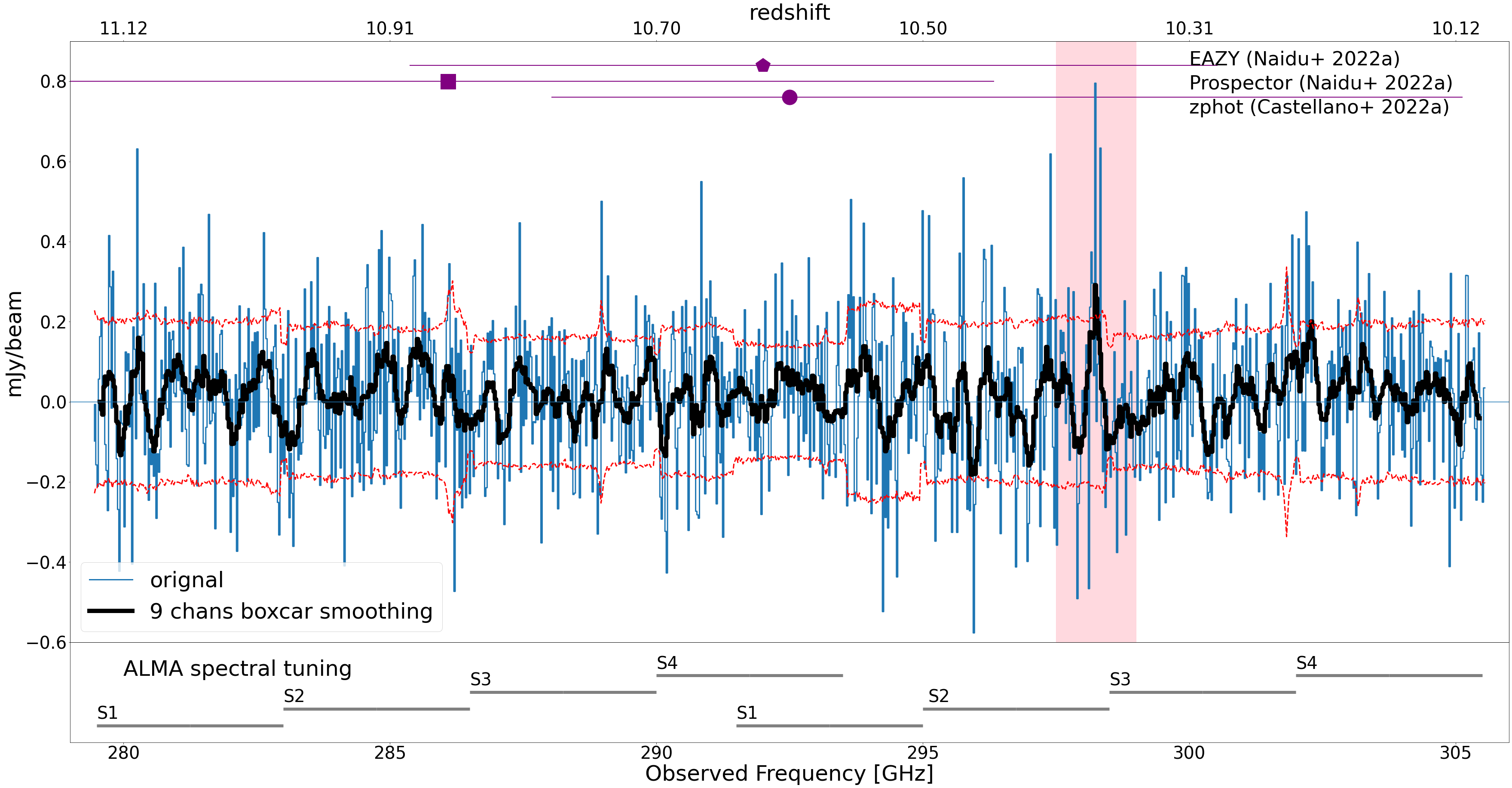
Figure 1: ALMA spectrum with 25 km s^-1 resolution at the location of GHZ1 (extracted from a single voxel with a unit of mJy beam^-1) for the full 26.125 GHz spectral frequency range. Three photo-$z$ estimates are shown by the purple symbols and horizontal lines. The bottom panel shows the spectral setup of our ALMA observation seamlessly covering the entire frequency range. The spectrum is extracted from ‘dirty’ cube without continuum subtraction. The blue line is the original spectrum and the black line is the spectrum with a boxcar smoothing using 9 channels. The red dashed line indicates $1\sigma$ RMS value at each spectral channel map and the spectrum highlighted by the pink shaded region that includes $\approx 4\sigma$ peak, is shown in Figure 2.

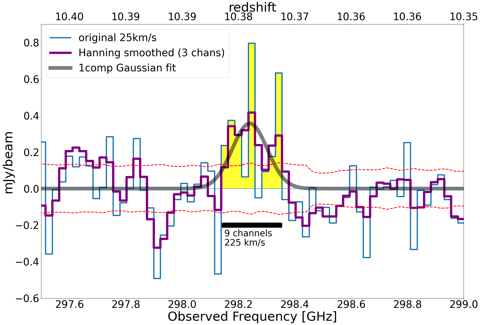
Figure 2: The zoomed-in ALMA spectrum highlighted by pink-colored box in Figure 1. In addition to the original spectrum (in blue), we show the Hanning smoothed spectrum (in purple) using 3 channels without decimating spectral channels. The red dashed line corresponds to $1\sigma$ RMS value at each spectral channel of the Hanning smoothed spectral cube. The black horizontal bar indicates the range of spectral channels (i.e., 9 channels) that is used to create a 225 km s^-1 resolution channel map in Figure 3(a). The thick solid gray line is the best fit 1-component Gaussian profile to the Hanning smoothed spectrum, with the velocity FWHM of 148 km s^-1.

4.2 Thermal dust continuum emission

The continuum emission at 292.5 GHz around the peak of the rest-frame FIR SED, is created by CASA multi-frequency synthesis imaging with nterms=1. We also do not find a significant ($>5\sigma$) continuum emission from GHZ1 while we observe a marginal $2.6\sigma$ continuum peak emission at the location of GHZ1 (Section 4.3). Interestingly, the FIR continuum is detected for other JWST galaxies in the ALMA field (Section 4.4).

4.3 Tentative line and continuum emission

Although we conclude that our ALMA observation does not detect a significant ($>5\sigma$) [$\textrm{O}\scriptstyle\mathrm{III}$]_88μm emission line and FIR continuum emission at the location of GHZ1, we find that there is a tentative ‘feature’ in the spectral cube and continuum map that might be associated with GHZ1. In Figure 3(a), we show the 225 km s^-1 resolution channel map at 298.25 GHz using 9 channels shown in Figure 2. In Figure 3(b), we show our 26.125 GHz bandwidth continuum map created from all execution blocks in our observation. The measurements of the fluxes and RMS noises for the line and continuum map are summarized in Table 2.

The collapsed channel map (Figure 3(a)) with $-1,1,2,3,4\sigma$ contour shows a $4.1\sigma$ peak emission (0.31 mJy beam^-1) at the location that is $0\arcsec.17$ away (to West) from GHZ1 seen in the JWST image on the right. The continuum map with $-1,1,2\sigma$ contour shows a $2.6\sigma$ peak emission (15.6 $\mu$Jy beam^-1) at the location that is also $0\arcsec.17$ away (to North) from GHZ1.

The $0\arcsec.17$ spatial offset from the GHZ1 is just a little larger than the ‘expected’ $1\sigma$ astrometric uncertainty of JWST pointing ($0.\arcsec 152$). The nominal RMS of ALMA absolute positional accuracy becomes poor if the peak signal-to-noise ratio of the target is low, and for our observation ($0.\arcsec 7$ beam and peak S/N$\sim 3$), it can be as large as $0.\arcsec 26$ based on the approximate relationship between the positional accuracy, beam size and target peak S/N (Remjian et al., 2019). Also, we found that the astrometric difference between ALMA and JWST is small (less than the size of one ALMA pixel, i.e., $<0.\arcsec 1$) based on the positional offset between the peak of the brightest ALMA continuum source in the field (shown in Figure 4 discussed in Section 4.4) and its JWST counterpart. Therefore we do not expect a systematic positional offset between ALMA and JWST, and this observed $0\arcsec.17$ offset is likely to be a result of the combination of the random astrometric uncertainty of JWST and ALMA.

Moreover, the observation of high-$z$ galaxies suggests that the [$\textrm{O}\scriptstyle\mathrm{III}$]_88μm emission (Carniani et al., 2017) as well as the dust continuum emission (Inami et al., 2022) can be spatially offset from the galaxy optical emission. Therefore, just based on the positional offset alone, we cannot exclude the association of this tentative ‘feature’ with the galaxy GHZ1.

However, as emphasized in the recent study of the analysis of the noise in the ALMA data cube, it is tempting to trust a $3\sim 4\sigma$ peak at the position where we expect to find it and we may be mistaken without testing how likely the peak is to be a noise fluctuation (Kaasinen et al., 2022). To assess the significance of the tentative emission seen in the collapsed map, with a $0.\arcsec 17$ spatial offset from the location of GHZ1, we did a simple investigation. First, we smoothed the 25 km s^-1 original spectral cube using a boxcar kernel with 5 different resolutions: 3, 5, 7, 9, and 11 channels (75, 125, 175, 225, and 275 km s^-1) as described in Section 3.3, and searched for the strongest feature around the location of GHZ1 within a radius of 1 FWHM of the beam (0.″7), for each spectral cube. We find that the spectral feature that we identified at 298.25 GHz in the original 25 km s^-1 resolution spectrum (Figure 1) still remains to be the strongest emission for all 5 resolutions. We confirm that a $4.1\sigma$ emission line (0.31 mJy beam^-1) at 225 km s^-1 resolution (Figure 3(a)) is the strongest emission, and this positive feature is 50% higher than any negative feature in the spectra.

Second, we compute the probability that a $4.1\sigma$ emission seen at 225 km s^-1 resolution channel map could be due to Gaussian noise within a radius of 1 FWHM of the beam (0.″7) from the galaxy position, by counting the number of independent samples (i.e., number of independent channels $\times$ number of independent beams) in frequency and spatially within the area with 1 beam radius ($\pi r_{\mbox{\tiny FWHM}}^{2}$) across the entire 26.125 GHz spectral range. The final cube with the full 26.125 GHz frequency range used for the analysis has 120 channels with 225 km s^-1 (0.216 GHz) per channel resolution and the spatial area for search is within a radius of 1 beam FWHM resulting in 3.14 beams. Therefore the total number of independent samples is $\approx 380$. The Gaussian probability for a noise feature above $4\sigma$ is $3.2\times 10^{-5}$. The product is then 0.012, which corresponds to the probability of seeing a $\geq 4\sigma$ noise feature over the number of independent samples, within the area of 1 beam FWHM radius. Therefore, the $4.1\sigma$ tentative emission we see from $0.\arcsec 17$ ($<1$ beam FWHM) away from GHZ1 has a 1.2% probability of being due to random Gaussian noise.

More rigorous analysis (e.g., Kaasinen et al., 2022) of the noise can be done to increase the reliability of the claim of detection, although, in general, an ALMA noise field in a region void of any significant emission (the brightest continuum emission from the source in the southern edge of the field seen in Figure 4 is only 87$\mu$Jy/beam, or $1.1\sigma$ at 225 km s^-1 channel^-1), is decidedly Gaussian in nature, dictated by the thermal noise of the system. Indeed, we performed an exercise of counting voxels with $>4\sigma$ or $<-4\sigma$ flux and computing their fraction out of the total number of voxels in the entire cube and found that the fractions ($3.2\times 10^{-5}$ for $>4\sigma$ voxels and $4.5\times 10^{-5}$ for $<-4\sigma$ voxels) are close to the Gaussian probability of $4\sigma$ ($3.2\times 10^{-5}$). However, there is also an increase in the required search space inherent in a multivariate analysis which includes a resolution in space and frequency. So while the 1.2% Gaussian noise probability at a specific spatial and spectral resolution seems low, we consider it optimistic, and it is certainly not low enough to claim a detection, but warrants further investigation.

Figure 3: Panel (a): 225 km s^-1 resolution channel map of the line feature associated with [$\textrm{O}\scriptstyle\mathrm{III}$]_88μm emission at 298.25 GHz observing frequency with -1 (dashed line), 1, 2, 3, 4 $\sigma$ contour (left) and JWST F444W NIRCam image of GHZ1 (right). The $4.1\sigma$ peak emission (0.31 mJy/beam) is $\approx 1.5$ ALMA pixels ($0\arcsec.17$) away (to West) from GHZ1 shown in the JWST NIRCam image (right). Panel (b): FIR continuum map at 292.5 GHz observing frequency with -1 (dashed line), 1 and 2 $\sigma$ contours. The peak continuum emission ($15.6\mu$Jy/beam) is also $\approx 1.5$ ALMA pixels ($0\arcsec.17$) away (to North) from GHZ1 shown in the JWST NIRCam image (right).

4.4 Serendipitous detection of other galaxies

We create the continuum image by running tclean on the continuum visibility identified by the ALMA pipeline. We detected FIR continuum emission from six sources in the ALMA field of view and these six FIR sources have NIR counterparts in the JWST NIRCam image (Figure 4). The photometric redshift of these galaxies ranges from $z=0.6$ to $z=3$ (Merlin et al., 2022). We found that 5 of them are not visible in the image created with robust=0.5, which indicates that the angular resolution for sufficient surface brightness sensitivity is very important to follow-up on the high-redshift JWST galaxies. The detailed information of the FIR flux and morphology of these sources, and the broadband SED analysis including the photometry from HST, JWST, and ALMA will be presented in a companion paper (Yoon et al. in preparation).

Figure 4: Left: ALMA continuum image at 292.5 GHz with the overlayed red contours range from 3 to 8$\sigma$ level increased by $1\sigma$ Right: JWST F444W NIRCam image of the galaxies in the ALMA field of view, with the contours of the ALMA continuum emission. ALMA detects FIR continuum emission from six galaxies denoted by numbers.

5 Discussion

We discuss the implications of the result from our observation. First, given the lack of significant ($>5\sigma$) [$\textrm{O}\scriptstyle\mathrm{III}$]_88μm emission line and thermal dust continuum emission from the location of GHZ1, we use the upper limit of the [$\textrm{O}\scriptstyle\mathrm{III}$]_88μm emission line and the continuum emission. Second, we use the measurement from the tentative emission. Lastly, we discuss the lessons from non-detection.

5.1 Upper-limit of [OIII] emission line

We derive the [$\textrm{O}\scriptstyle\mathrm{III}$]_88μm luminosity from the velocity-integrated line flux density ($S\Delta v$ in Jy km s^-1) using $L_{\mbox{\scriptsize line}}=1.04\times 10^{-3}S\Delta vD^{2}_{\mbox{\tiny}L}\nu_{\mbox{\scriptsize obs}}[L_{\odot}]$ (Carilli & Walter, 2013) where $D_{\mbox{\tiny}L}$ is luminosity distance in Mpc and $\nu_{\mbox{\scriptsize obs}}$ is observed frequency in GHz. For the line luminosity, we used the best photo-$z$ estimate ($z=10.60$ corresponding to 292.5 GHz observing frequency) and assume that the line is observed at the center frequency (292.5 GHz) of the full frequency range. The velocity integrated flux density ($S\Delta v$) and the [$\textrm{O}\scriptstyle\mathrm{III}$]_88μm luminosity ($L_{[\mbox{\tiny OIII}]}$) are in Table 2.

Using the $5\sigma$ upper limit of [$\textrm{O}\scriptstyle\mathrm{III}$]_88μm luminosity ($2.06\times 10^{8}L_{\odot}$) with assumed 148 km s^-1 velocity FWHM from the Gaussian fit (Figure 2) and the star formation rate (SFR=$10.8^{+50.3}_{-6.1}$ M_⊙yr^-1) inferred from the galaxy SED modeling using NIRCam photometry (Castellano et al., 2022b), we present the SFR-$L_{[\mbox{\tiny OIII}]}$ relation in Figure 5. The blue and orange line with a $1\sigma$ shaded-color region in Figure 5 shows the SFR-$L_{[\mbox{\tiny OIII}]}$ relation for low-metallicity dwarf galaxies and starburst galaxies (De Looze et al., 2014) and the red dot-dashed line is the best-fit relation for a handful of high-$z$ galaxies (Harikane et al., 2020). The $5\sigma$ upper limit of GHZ1 is shown by the blue star symbol with the SFR error bar. The blue ‘x’ symbol without an associated error bar shows the sum of ‘obscured’ IR SFR (using Equation (1) in Hayward et al., 2014) determined by the IR luminosity output from the SED model and ‘unobscured’ UV SFR determined by the UV luminosity (using Equation (4) in Rosa-González et al., 2002). For comparison, we also plot the values of GHZ2 (Bakx et al., 2023): $5\sigma$ upper limit at the location of GHZ2 in the JWST image (blue circle) and the $5.8\sigma$ detection from 0.″5 away from GHZ2 (red circle) with the SFR error bar.

The [$\textrm{O}\scriptstyle\mathrm{III}$]_88μm upper limit for GHZ1 follows the SFR-$L_{[\mbox{\tiny OIII}]}$ relation for metal-poor dwarf galaxies. However, given that it is an upper limit, we cannot rule out a scenario that GHZ1 is consistent with the starburst galaxies (orange line in Figure 5) although it is less likely.

5.2 Upper-limit of thermal dust continuum emission

Based on the $3\sigma$ upper limit of the 292.5 GHz continuum flux density and the JWST NIRCam photometry at F150W,F200W,F277W,F356W,F444W, we create the spectral energy distribution (SED) model of GHZ1 using CIGALE (Boquien et al., 2019) that computes a self-consistent SED from optical/NIR to FIR based on the amount of energy absorbed by dust (determined by dust extinction, $A_{V}=R_{V}E(B-V)$) and has been used to investigate the properties of dust in early galaxies (e.g., Burgarella et al., 2020). We adopt the SED parameters ($e$-folding time scale for star formation history, stellar population age, stellar mass, $E(B-V)$) based on the NIRCam-only photometry (Merlin et al., 2022) for CIGALE and use single dust temperature graybody (dust emissivity $\beta=1.6$) model (Casey, 2012) for FIR SED.

For our modeling, we incorporate the systematic effects of CMB as a thermal background: an additional heating source and a reduced contrast against the background which become significant with increasing redshift as presented by the previous studies (e.g., da Cunha et al., 2013; Zhang et al., 2016). Instead of adopting the conventional approach that uses FIR-only SED from a graybody function with a normalization from dust mass and compares it to the observed photometry corrected for the CMB effect, we choose to perform a full forward SED modeling. Although the full SED modeling based on energy balance has its own limitations due to parameter degeneracy and strong assumptions that may not always represent the reality (e.g., Buat et al., 2019), it is still useful because the use of single FIR photometry cannot constrain the dust parameter (temperature and mass) and the JWST photometry helps to constrain the overall energy budget in FIR if the energy balance assumption (valid for compact and co-spatial IR and optical emission) holds for GHZ1, which is likely because of its extended regular disk-like morphology (Naidu et al., 2022a).

Using CIGALE, we create a galaxy SED using graybody FIR spectrum with dust temperature increased by CMB heating following the same procedure in da Cunha et al. (2013). Since the ‘initial’ model SED from CIGALE does not have the contribution from CMB heating, we add an additional graybody spectrum with the CMB temperature at a given redshift to the model SED and apply the correction factor due to the CMB contrast (da Cunha et al., 2013). We note that the dust temperature and the mass are not independent, for the fixed IR luminosity (see Equation A8): if we choose the dust temperature as a free parameter, the dust mass is determined, and vice versa. The detailed description of our SED modeling including the CMB effect is described in Appendix A.

Figure 6 shows the SED models of GHZ1 obtained by varying SED with dust temperature and using $A_{V}=0.48$ that was chosen to match the observed JWST NIRCam photometry (black dots) by Santini et al. (2023). The total IR luminosity is determined by the dust-absorbed energy and the FIR SED shape is determined by the assumed dust temperature. Depending on the assumed dust temperature $T_{d}(0)$ without being affected by CMB heating at $z=10.60$, FIR SED can vary significantly without changing the NIR SED shape. Although it is not possible to obtain a reliable dust temperature by modeling a single FIR photometry, the best SED model prefers the FIR SED with a 90 K dust (with the corresponding $\approx 10^{4}M_{\odot}$ dust mass) for our $3\sigma$ upper limit of FIR continuum emission at 292.5 GHz.

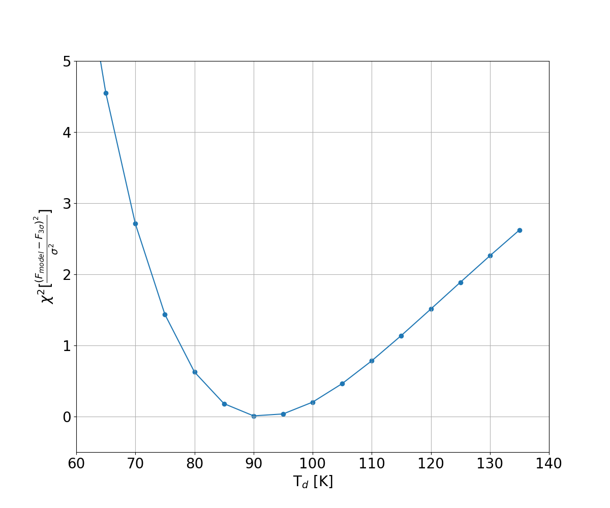
Figure 7: $\chi^{2}$ value as a function of dust temperature. A single minimum value is observed at around $T_{d}(0)=90$K with a corresponding dust mass, $M_{d}=10^{4}M_{\odot}$.

In Figure 7, we compute a $\chi^{2}$ value ($\chi^{2}=(F_{\mbox{\tiny model}}-F_{3\sigma})^{2}/\sigma^{2}$) of the model SED evaluated at the $3\sigma$ upper limit of the continuum flux density at 292.5 GHz, as a function of dust temperature. We note that the $\chi^{2}$ value estimated based on “one” data point does not have a strong statistical implication on the model parameter (i.e., dust temperature). However, Figure 7 shows that there is a single minimum value of $\chi^{2}$ at $T_{d}=90$K and the $3\sigma$ upper limit clearly disfavors the dust temperature that is significantly lower than 90K.

The result implies that GHZ1 has very little dust with small ($\approx 10^{-5}$) dust-to-stellar mass ratio significantly lower than the typical values (e.g., $10^{-2}\sim 10^{-3}$ in Calura et al., 2017). The small amount of dust in GHZ1 can be explained by dust ejection due to energetic star formation in the early Universe as suggested by the recent literature (e.g., Ferrara et al., 2022; Fiore et al., 2023; Nath et al., 2022; Ziparo et al., 2023). Also, the high dust temperature of GHZ1 is in line with the observational studies showing that the dust temperature of high-$z$ galaxies is higher than the local galaxies (e.g., Bakx et al., 2020, 2021; Faisst et al., 2020; Liang et al., 2019; Schouws et al., 2022), which supports for the low dust-to-gas ratio of high-$z$ galaxies (Hirashita & Chiang, 2022). Theoretical studies also suggest the increasing dust temperature with redshift (Behrens et al., 2018; Sommovigo et al., 2021, 2022). We note that the dust temperature estimate based on $3\sigma$ continuum upper limit is only a lower limit and can be even higher than 90K if the continuum emission is detected at a level below the current $3\sigma$ RMS.

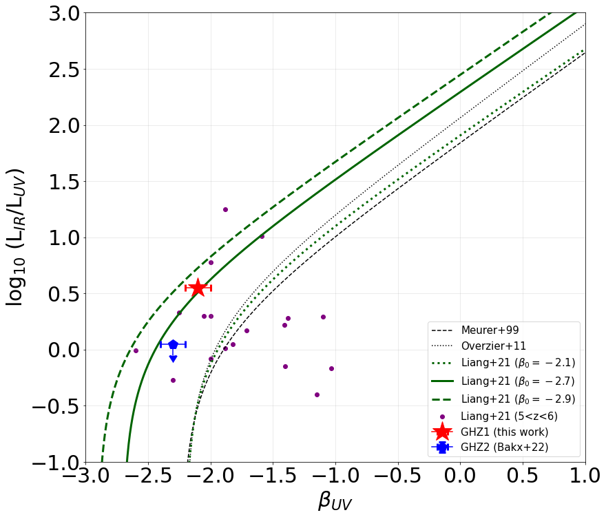
Figure 8: IRX-$\beta$ relation for GHZ1 and GHZ2 with the distribution of the high-redshift ($5<z<6$) galaxies (purple dots) complied by Liang et al. (2019) and their model relation with different intrinsic UV slopes ($\beta_{0}=-2.1,-2.7,-2.9$ shown by the green thick lines), and the reference relation from Meurer et al. (1999) (black dashed line) and Overzier et al. (2011) (black dotted line).

Also we locate GHZ1 in the IRX-$\beta_{\mbox{\tiny UV}}$ relation (Figure 8) where IRX$={L_{\mbox{\tiny IR}}}/{L_{\mbox{\tiny UV}}}$ and $\beta_{\mbox{\tiny UV}}$ is the UV continuum slope. The IR luminosity is estimated by integrating CIGALE SED for 8-1000$\mu$m rest-frame wavelength range and the UV luminosity is estimated based on $M_{\mbox{\tiny UV}}=-21.0$ (Naidu et al., 2022a; Castellano et al., 2022a). We use $\beta_{\mbox{\tiny UV}}=-2.1\pm 0.1$ (Naidu et al., 2022a). Figure 8 shows two IRX-$\beta_{\mbox{\tiny UV}}$ relations from Meurer et al. (1999) (black dashed line) and Overzier et al. (2011) (black dotted line) as a reference, and the distribution of high-redshift galaxies (purple dots) complied by Liang et al. (2019). The observed scatter of the galaxies in the IRX-$\beta_{\mbox{\tiny UV}}$ relation arises from the variations in the intrinsic UV spectral slope ($\beta_{0}$) and the shape (in particular, the slope (Salim & Boquien, 2019)) of the dust attenuation curve (see Salim & Narayanan, 2020, and the reference therein). A variation of the slope of dust attenuation curve changes the tilt of the IRX-$\beta_{\mbox{\tiny UV}}$ relation (e.g., Salim & Boquien, 2019) and a variation of the intrinsic UV slope shifts the IRX-$\beta_{\mbox{\tiny UV}}$ model curve horizontally (e.g., Liang et al., 2019). For a simple dust slab model applied for simulated high-redshift galaxies, Liang et al. (2019) found that the intrinsic UV slope ($\beta_{0}$) of galaxies largely explains the scatter in the IRX-$\beta_{\mbox{\tiny UV}}$ relation.

In Figure 8, we also show three IRX-$\beta_{\mbox{\tiny UV}}$ relations from Liang et al. (2019) using Milky Way dust attenuation curve with different $\beta_{0}$ (from the same value as the observed one to the bluer slope $\beta_{0}<-2.1$ as shown by green thick dotted, solid and dashed line). The locations of GHZ1 and GHZ2 in the IRX-$\beta_{\mbox{\tiny UV}}$ plane are shown by red star and blue pentagon symbol respectively. We find that the use of IRX-$\beta_{\mbox{\tiny UV}}$ relation in Liang et al. (2019) with a bluer intrinsic UV slope (assumed to be $\beta_{0}=-2.7$) and the observed UV slope $\beta_{\mbox{\tiny UV}}=-2.1$ predicts the measured IRX value ($L_{\mbox{\tiny IR}}$ from CIGALE model SED and $L_{\mbox{\tiny UV}}$ from the observed JWST photometry) of GHZ1 well, which is consistent with the nature of GHZ1 (i.e., blue Lyman break galaxy at $z\approx 10$).

5.3 Measurement from the tentative line and continuum emission

We also measure the line luminosity and the continuum flux density (reported in Table 2) from the tentative feature in Section 4.3, using the line channel map and continuum map (Figure 3) and add them in Figure 5 and 6. The line measurement is performed using a circular aperture with a radius of $0.\arcsec 74$ (comparable to $4\times$ALMA beam area) to enclose the extended emission and the continuum measurement is performed using a circular aperture with a radius of $0.\arcsec 35$ (comparable to $1\times$ALMA beam area). The measurement error of the aperture photometry reported in Table 2 is the standard deviation of the flux density sampled with the same aperture from randomly selected 1000 positions (avoiding the region with continuum emission) in the field of view.

The [$\textrm{O}\scriptstyle\mathrm{III}$]_88μm luminosity of the tentative line emission at 298.25 GHz measured from the 225 km s^-1 resolution channel map (Figure 3(a)) is $2.83^{+0.83}_{-0.83}\times 10^{8}L_{\odot}$. The red star symbol with SFR and its error inferred from SED modeling (Castellano et al., 2022b) and the red ‘x’ symbol with the sum of ‘obscured’ and ‘unobscured’ SFR in the SFR-$L_{[\mbox{\tiny OIII}]}$ relation (Figure 5) are based on the [$\textrm{O}\scriptstyle\mathrm{III}$]_88μm luminosity from the tentative emission feature. They are consistent with the SFR-$L_{[\mbox{\tiny OIII}]}$ relation for the metal-poor dwarf galaxies, which may suggest that GHZ1 is metal-poor (also alluded by the low dust content inferred from the SED analysis) and has low ionization parameter that decreases the strength of [$\textrm{O}\scriptstyle\mathrm{III}$]_88μm emission (Kohandel et al., 2023).

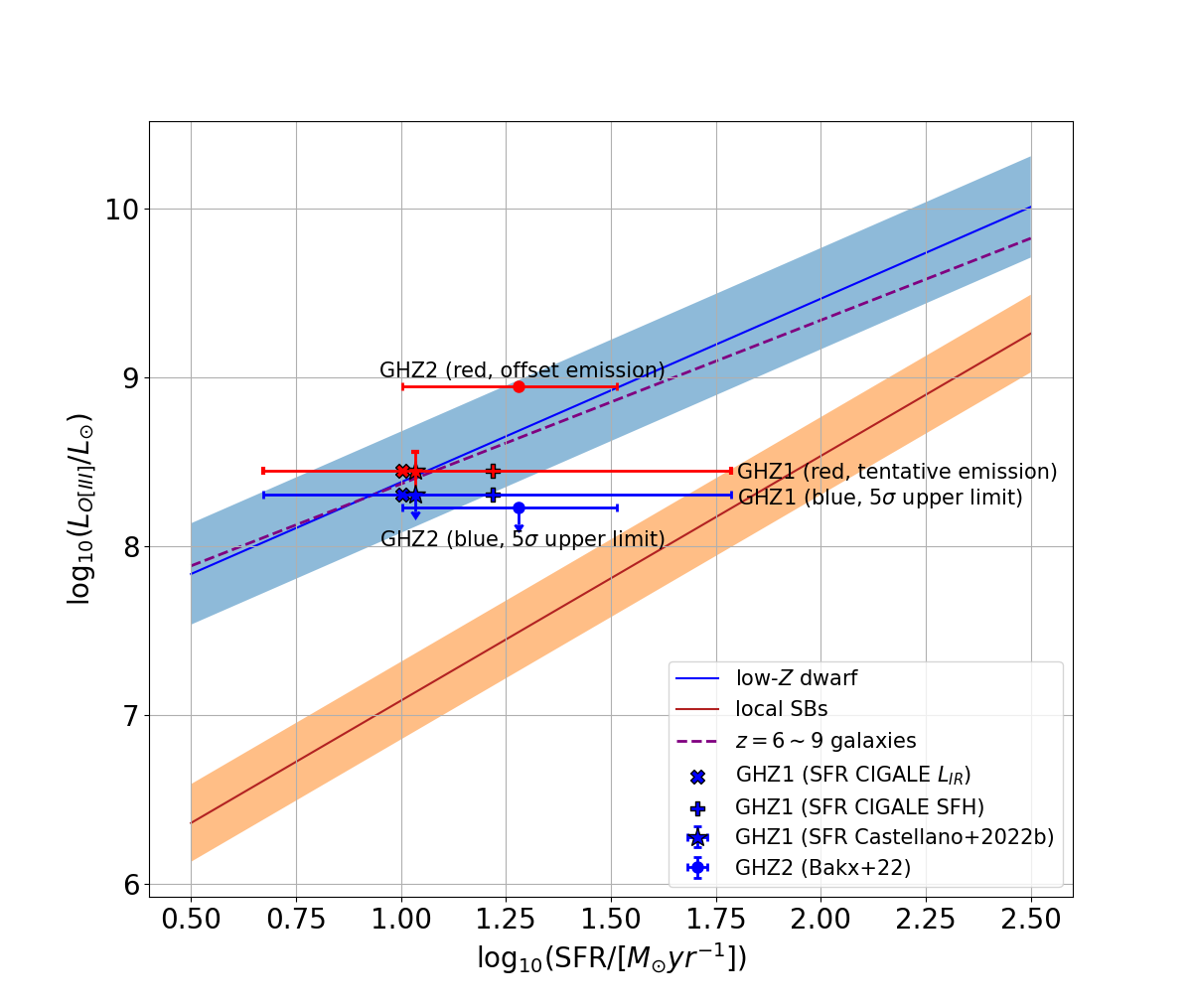
Figure 5: The SFR and [$\textrm{O}\scriptstyle\mathrm{III}$]_88μm luminosity relation. The relation for the low metallicity dwarf galaxies (blue line) and for the starburst galaxies (orange line) with a $1\sigma$ shaded-color region are from De Looze et al. (2014), and the best-fit relation (purple dashed line) for a handful of high-redshift galaxies is from Harikane et al. (2020). Two galaxies observed by ALMA: GHZ2 by Bakx et al. (2023) and GHZ1 (this work) with the $5\sigma$ upper limit of the [$\textrm{O}\scriptstyle\mathrm{III}$]_88μm luminosity, are shown by the black filled circle (GHZ2) and the black filled star (GHZ1). The [$\textrm{O}\scriptstyle\mathrm{III}$]_88μm luminosity for GHZ1 from the tentative emission is shown by the red filled star. The ‘x’ symbol is for the SFR estimated by the sum of the SFR traced by IR (obscured SF) and UV (unobscured SF). The [$\textrm{O}\scriptstyle\mathrm{III}$]_88μm luminosity for GHZ2 from the offset position (0.″5 offset from the JWST position) is shown by the red filled circle.

Modeling the Hanning smoothed spectrum (purple line in Figure 2) of the tentative line emission, using single Gaussian profile results in the center frequency of 298.24 GHz ($z=10.38$) and the velocity FWHM of 148 km s^-1 which is consistent with the FWHM values of the observed [$\textrm{O}\scriptstyle\mathrm{III}$] line (50-320 km s^-1) from other similarly high-redshift ($z\approx 8-9$) galaxies (Inoue et al., 2016; Laporte et al., 2017, 2021; Hashimoto et al., 2018; Tamura et al., 2019).

The continuum flux density from the tentative continuum emission (8.6 $\mu$Jy) is shown by the red star symbol (Figure 6). The tentative continuum emission prefers even higher dust temperature ($T_{d}>90$K) or, in other words, smaller dust mass ($M_{d}<10^{4}M_{\odot}$). The continuum upper limit and the tentative continuum emission suggest that given the non-negligible dust extinction value ($A_{V}=0.48$) to explain the JWST NIRCam photometry, the continuum flux density at 292.5GHz is lower than the expectation for a conventionally assumed dust temperature ($\approx 50$K) at high-$z$ Universe (e.g., $z\approx 7$ galaxies in Bakx et al., 2021; Sommovigo et al., 2022), which implies that the trend of increasing dust temperature at high-redshift may continue up-to $z\approx 10$ and beyond.

5.4 What we learn from a non-detection

Recently another ALMA observation (2021.A.00020.S, PI: Bakx) of a $z\gtrsim 10$ galaxy candidate, GHZ2, also reports the non-detection of [$\textrm{O}\scriptstyle\mathrm{III}$]_88μm emission and continuum emission (Bakx et al., 2023; Popping, 2023). It turns out that the first two ALMA programs for spectroscopic confirmation of the redshift of these high-$z$ galaxy candidates discovered by JWST, do not detect a significant emission at the location of the galaxy.

The non-detection of [$\textrm{O}\scriptstyle\mathrm{III}$]_88μm emission line can be explained by (1) insufficient line sensitivity, (2) ‘true’ galaxy redshift much lower than $z\sim 10$ (i.e., a low redshift interloper), or (3) the spectral coverage that is not wide enough to incorporate the full range of the photometric redshift probability distribution, as discussed by Bakx et al. (2023) and Popping (2023). The second scenario can be ruled out for GHZ1 because the drop-out at F115W is too extreme, and the detected continuum is too blue, to be explained by the low-redshift Balmer break or strong dust obscuration of UV emission. The FIR continuum upper limit or the tentative continuum emission does not allow an extremely high dust extinction to mimic the F115W drop-out, using a low-$z$ SED model, which also helps to rule out the second scenario. The third scenario can be ruled out if ALMA has a wider-band and higher-sensitivity correlator in near future (Carpenter et al., 2020). Like GHZ2, the insufficient sensitivity seems to be a plausible reason for the non-detection which can be explained by a low-metallicity interstellar medium (Bakx et al., 2023; Popping, 2023) or low-ionization parameter $U_{\mbox{\tiny ion}}$ in high-density environment (Kohandel et al., 2023).

Like GHZ2, the non-detection of continuum emission from GHZ1 can be attributed to the low dust production rate (Bakx et al., 2023) or the dust ejection due to energetic feedback (Ferrara et al., 2022; Fiore et al., 2023; Nath et al., 2022; Ziparo et al., 2023). However, it is not clear what is responsible for the non-detection of the continuum emission from GHZ1. Given that the energy balance SED model with the upper limit possibly suggests a high temperature ($T_{d}>90$K) and small mass ($M_{d}<10^{4}M_{\odot}$) dust, we need to have multiple FIR flux measurements at different frequencies to constrain the dust properties (mass, temperature, power-law slope of the Rayleigh-Jeans tail) of GHZ1 in order to understand the reason for the weak FIR continuum emission and more importantly to have an insight on the dust formation physics in the early Universe.

Based on our analysis, there is a tentative ‘feature’ in the spectral cube around 298.25 GHz sky-frequency (suggesting $z=10.38$) and the continuum image, that is likely to be associated with GHZ1. Given the lack of sufficient sensitivity, a further follow-up observation combined with the current observation is necessary to increase the S/N and confirm the tentative ‘feature’ in our data.

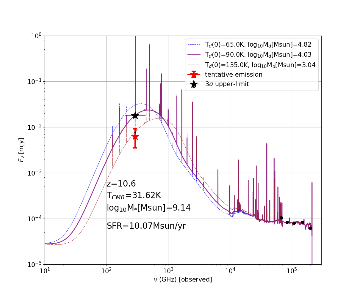
Figure 6: SED models for GHZ1 based on the near-IR photometry (black dots) from JWST NIRCam and the $3\sigma$ upper limit (black star) of FIR photometry from ALMA, with the inclusion of CMB effect (see Appendix A for more details). The best SED model suggests $T_{d}(0)=90$K and $M_{d}=10^{4}M_{\odot}$.

6 Summary

Our ALMA DDT program (2021.A.00023.S) observed a $z\gtrsim 10$ galaxy candidate, GHZ1, in the GLASS-JWST field to confirm its spectroscopic redshift using [$\textrm{O}\scriptstyle\mathrm{III}$]_88μm emission line. We find no clear $>5\sigma$ detection of the line and continuum emission at the location of GHZ1, but report a tentative emission ‘feature’ in the spectral cube ($4.1\sigma$ in the 225 km s^-1 resolution channel map) and continuum map ($2.6\sigma$) at a location close ($0.\arcsec 17$ away) to GHZ1, that might be associated with GHZ1. If the line is real and identified at [$\textrm{O}\scriptstyle\mathrm{III}$]_88μm, it would imply $z=10.38$ which agrees with the photo-$z$ within its $1\sigma$ uncertainty. The $5\sigma$ upper limit of the [$\textrm{O}\scriptstyle\mathrm{III}$]_88μm line emission and the inferred SFR suggest that GHZ1 in the SFR-$L_{[\mbox{\tiny OIII}]}$ plane is consistent with the metal-poor dwarf galaxies and the several observed high-$z$ galaxies. The SED modeling based on the $3\sigma$ upper limit of the continuum emission and the JWST NIRCam photometry suggests that GHZ1 has a small fraction ($\lesssim 10^{-5}$ of stellar mass) of hot dust ($T_{d}\gtrsim 90$K). We need a confirmation of the tentative emission to have a firm conclusion. Finally, we also report six serendipitous FIR sources with the JWST galaxy counterpart, of which properties will be presented in a separate paper.

Although we report no clear detection of [$\textrm{O}\scriptstyle\mathrm{III}$]_88μm emission line, the initiative of the ALMA FIR observation of the $z\gtrsim 10$ galaxy candidates discovered by JWST is an important step to improve our understanding of the galaxy population and ISM condition in the formation epoch of first galaxies.

Appendix A Computing Observed FIR SED with the inclusion of CMB effect

The effect of CMB on the observation of thermal dust emission is twofold. CMB affects the FIR SED by enhancing the thermal blackbody component of the FIR SED (i.e., heating) but also by reducing the contrast of the detection (i.e., strong background emission). Therefore the ‘observed’ FIR SED shape deviates from the $z=0$ SED with increasing redshift and the CMB effect (i.e., heating and contrast against the background) needs to be included when we model the SED. The basic theoretical framework and the prescription for the correction of CMB to the FIR SED model are described in da Cunha et al. (2013). Here we reformulate the prescription in da Cunha et al. (2013) to include the normalization of IR luminosity and describe how we implement it into a panchromatic SED model (UV-to-FIR) from CIGALE.

To consider the CMB heating, we add an additional IR luminosity from dust heated by CMB at redshift $z$ to the modified blackbody SED component of FIR SED created by CIGALE. For high-redshift observations (Scoville, 2013),

$$\nu_{obs}S_{\nu_{obs}}=\nu_{rest}\frac{L_{\nu_{rest}}}{4\pi D_{L}^{2}}$$ (A1)

with $\nu_{rest}=\nu_{obs}\times(1+z)$. Using dust mass ($M_{dust}$) and mass absorption coefficient ($\kappa_{\nu}$),

$$S_{\nu_{obs}}=(1+z)\kappa_{\nu_{rest}}4\pi B_{\nu_{rest}}(T)\frac{M_{dust}}{4\pi D_{L}^{2}}$$ (A2)

Therefore,

$$L_{\mbox{\tiny IR}}=\int 4\pi D_{L}^{2}S_{\nu_{obs}}d\nu_{obs}=\int\kappa_{\nu_{rest}}4\pi B_{\nu_{rest}}(T)M_{dust}d\nu_{rest}$$ (A3)

where

$$\kappa_{\nu_{rest}}=\kappa_{0}\left(\frac{\nu_{rest}}{\nu_{0}}\right)^{\beta}$$ (A4)

with the reference value $\kappa_{0}$ at a reference frequency $\nu_{0}$ that can adopted from observations. Then $L_{\mbox{\tiny IR}}$ from dust with temperature $T$ can be written as

$$L_{\mbox{\tiny IR}} = \int\kappa_{\nu_{rest}}4\pi B_{\nu_{rest}}(T)M_{dust}d\nu_{rest}$$ (A5)

$$= 4\pi\frac{2h\nu_{0}^{4}}{c^{2}}\left(\frac{kT}{h\nu_{0}}\right)^{4+\beta}\kappa_{0}M_{dust}\int_{0}^{\infty}\frac{x^{3+\beta}}{e^{x}-1}dx$$

where $x\equiv\frac{h\nu_{rest}}{kT}$. Riemann-zeta function $\zeta(s)$ is

$$\zeta(s)=\frac{1}{\Gamma(s)}\int_{0}^{\infty}\frac{x^{s-1}}{e^{x}-1}dx$$ (A6)

where $\Gamma(s)=\int_{0}^{\infty}x^{s-1}e^{-x}$ is the gamma function. Therefore, using the values of the physical constants, the above equation is re-written as

$$L_{\mbox{\tiny IR}} = 4\pi\frac{2h\nu_{0}^{4}}{c^{2}}\left(\frac{kT}{h\nu_{0}}\right)^{4+\beta}\kappa_{0}M_{dust}\zeta(4+\beta)\Gamma(4+\beta)$$ (A7)

$$= 3.355\times 10^{28}\left(\frac{\nu_{0}}{20.809~{}\mbox{\small GHz}}\right)^{-\beta}\left(\frac{T}{\mbox{K}}\right)^{4+\beta}\left(\frac{\kappa_{0}}{0.484~{}\mbox{cm}^{2}\mbox{g}^{-1}}\right)\left(\frac{M_{dust}}{M_{\odot}}\right)\zeta(4+\beta)\Gamma(4+\beta)\quad[\mbox{erg s}^{-1}]$$

where $\nu_{0}$ is in GHz and $\kappa_{0}$ is in cm² g^-1. We adopt ${\nu_{0}}=352.697$GHz (or 850$\mu$m) and $\kappa_{0}=0.484$ cm² g^-1 from Cochrane et al. (2022). Using the emissivity index $\beta=1.6$, we obtain $L_{\mbox{\tiny IR}}$ in the unit of Watt (used in CIGALE)

$$L_{\mbox{\tiny IR}}=2.29\times 10^{21}~{}\left(\frac{T}{\mbox{K}}\right)^{5.6}\left(\frac{M_{dust}}{M_{\odot}}\right)\quad[\mbox{W}]$$ (A8)

For the fixed $L_{\mbox{\tiny IR}}$, the higher the dust temperature is, the less the dust mass is.

If assuming thermal equilibrium, CMB provides additional heating to dust and this CMB heating becomes significant with increasing redshift. For CMB temperature at redshift, $T_{\mbox{\tiny CMB}}(z)$, the IR luminosity from CMB heating is

$$L^{\mbox{\tiny CMB}}_{\mbox{\tiny IR}}=2.29\times 10^{21}~{}\left(\frac{T_{\mbox{\tiny CMB}}(z)}{\mbox{K}}\right)^{5.6}\left(\frac{M_{dust}}{M_{\odot}}\right)\quad[\mbox{W}]$$ (A9)

Because of the CMB heating, the dust temperature increases with redshift. Based da Cunha et al. (2013), we infer the dust temperature, $T_{d}(z)$ at a given redshift $z$ from

$$T_{d}^{4+\beta}(z)=T_{d}^{4+\beta}(0)-T_{\mbox{\tiny CMB}}^{4+\beta}(0)+T_{\mbox{\tiny CMB}}(0)^{4+\beta}\times(1+z)^{4+\beta}$$ (A10)

where $T_{\mbox{\tiny CMB}}(0)=2.725$K for the standard $\Lambda$CDM cosmology and $T_{d}(0)$ is the dust temperature at $z=0$.

For galaxy SED at $z$, we use CIGALE that assumes the energy balance: the energy created by the underlying stellar population is absorbed by the dust following the dust attenuation curve and the absorbed luminosity is re-emitted in FIR. For FIR SED module, we use a modified black body function with the elevated dust temperature $T_{d}(z)$ (Equation A10). However, we note that the resulting FIR SED from CIGALE does not include the CMB heating. We need to add $L^{\mbox{\tiny CMB}}_{\mbox{\tiny IR}}$ to the normalization of the CIGALE FIR SED which we can compute numerically. If we write the normalization of the CIGALE FIR SED for $T_{d}(z)$ without CMB heating included, $L^{\mbox{\tiny abs}}_{\mbox{\tiny IR}}$, the ‘boosted’ IR SED can be obtained by correcting the CIGALE FIR SED with $T_{d}(z)$ by multiplying $(L^{\mbox{\tiny abs}}_{\mbox{\tiny IR}}+L^{\mbox{\tiny CMB}}_{\mbox{\tiny IR}})/L^{\mbox{\tiny abs}}_{\mbox{\tiny IR}}$.

Now the ‘boosted’ FIR luminosity, $L^{\mbox{\tiny tot}}_{\mbox{\tiny IR}}$, (due to the CMB heating) with elevated dust temperature $T_{d}(z)$ is the sum of $L^{\mbox{\tiny abs}}_{\mbox{\tiny IR}}$ and $L^{\mbox{\tiny CMB}}_{\mbox{\tiny IR}}$ and can be written as

$$L^{\mbox{\tiny tot}}_{\mbox{\tiny IR}} = 2.29\times 10^{21}~{}\left(\frac{T_{d}(z)}{\mbox{K}}\right)^{5.6}\left(\frac{M_{dust}}{M_{\odot}}\right)$$ (A11)

$$= 2.29\times 10^{21}~{}\left(\frac{T_{\mbox{\tiny CMB}}(z)}{\mbox{K}}\right)^{5.6}\left(\frac{M_{dust}}{M_{\odot}}\right)+L^{\mbox{\tiny abs}}_{\mbox{\tiny IR}}$$

This results in a dust mass consistent with the luminosity balance: $L^{\mbox{\tiny tot}}_{\mbox{\tiny IR}}=L^{\mbox{\tiny CMB}}_{\mbox{\tiny IR}}+L^{\mbox{\tiny abs}}_{\mbox{\tiny IR}}$

$$\left(\frac{M_{dust}}{M_{\odot}}\right)=\frac{L^{\mbox{\tiny abs}}_{\mbox{\tiny IR}}}{2.29\times 10^{21}\left[\left(\frac{T_{d}(z)}{\mbox{K}}\right)^{5.6}-\left(\frac{T_{\mbox{\tiny CMB}}(z)}{\mbox{K}}\right)^{5.6}\right]}$$ (A12)

In our procedure for computing the ‘boosted’ FIR SED by CMB heating, we numerically compute $L^{\mbox{\tiny abs}}_{\mbox{\tiny IR}}$ from the CIGALE FIR SED and estimate $M_{dust}$ for given $T_{d}(z)$ and $T_{\mbox{\tiny CMB}}(z)$. Then $L^{\mbox{\tiny CMB}}_{\mbox{\tiny IR}}$ is computed and the CIGALE FIR SED is multiplied by $(L^{\mbox{\tiny abs}}_{\mbox{\tiny IR}}+L^{\mbox{\tiny CMB}}_{\mbox{\tiny IR}})/L^{\mbox{\tiny abs}}_{\mbox{\tiny IR}}$. This is equivalent to scale the FIR SED model by multiplying a scale factor $\left(\frac{T_{d}(z)}{T_{d}(0)}\right)^{4+\beta}$ (da Cunha et al., 2013).

The other aspect of CMB effect is the suppression of SED because the ‘observed’ SED is against the background emission from CMB. Following da Cunha et al. (2013), we apply the correction factor, $1-\{B_{\nu}\left[T_{\mbox{\tiny CMB}}(z)\right]/B_{\nu}\left[T_{d}(z)\right]\}$ to the modified blackbody component of the ‘boosted’ FIR SED.

Figure 9 shows the SEDs of a galaxy with $M_{*}=1.5\times 10^{10}M_{\odot}$ and dust temperature $T_{d}(0)=35$K for three different cases: (1) the gray line shows a SED with ‘elevated’ dust temperature $T_{d}(z)=36.4$K due to the CMB heating at $z=9$ (Equation A10) but without having the CMB heating and contrast yet, (2) the blue line shows the same SED including the additional FIR energy from CMB heating with $T_{\mbox{\tiny CMB}}=27.26$K at $z=9$, and (3) the purple line shows the SED after correcting the CMB contrast. The dashed line for each color shows the modified blackbody (MBB) SED component for each case.

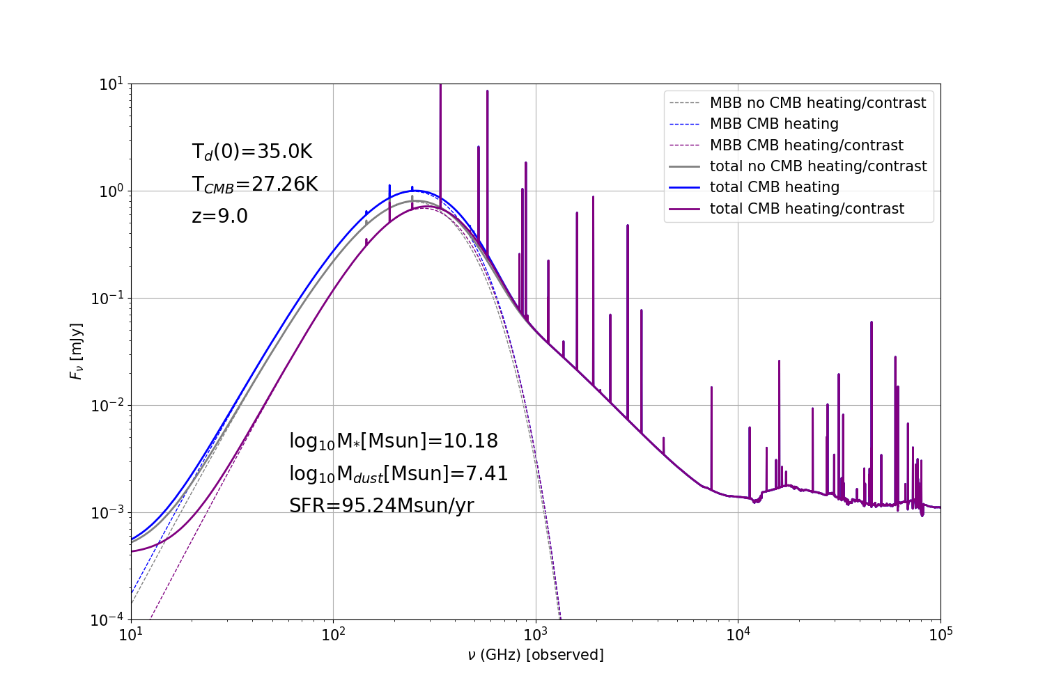
Figure 9: Illustration of the creation of model SED with the inclusion of CMB effect. The SED of a model galaxy with $M_{*}=1.5\times 10^{10}M_{\odot}$ and SFR=95$M_{\odot}$/yr is created by CIGALE using conventional ‘delayed’ SFH and 36.4K dust temperature at $z=9$ (gray solid line) with 35K dust temperture at $z=0$. Then the additional heating from CMB with $T_{\mbox{\tiny CMB}}=27.26$K at $z=9$ is applied to the modified blackbody function of the SED (blue dashed line), and the modified blackbody function with $T_{\mbox{\tiny CMB}}$ is subtracted to take the background contrast into account (purple dashed line). The ‘net’ SED shown by purple solid line, after taking the CMB effect into account, is the model of an ‘observed’ galaxy SED at high redshift Universe.

References

- Adams et al. (2023) Adams, N. J., Conselice, C. J., Ferreira, L., et al. 2023, MNRAS, 518, 4755, doi: 10.1093/mnras/stac3347
- Atek et al. (2023) Atek, H., Shuntov, M., Furtak, L. J., et al. 2023, MNRAS, 519, 1201, doi: 10.1093/mnras/stac3144
- Bakx et al. (2020) Bakx, T. J. L. C., Tamura, Y., Hashimoto, T., et al. 2020, MNRAS, 493, 4294, doi: 10.1093/mnras/staa509
- Bakx et al. (2021) Bakx, T. J. L. C., Sommovigo, L., Carniani, S., et al. 2021, MNRAS, 508, L58, doi: 10.1093/mnrasl/slab104
- Bakx et al. (2023) Bakx, T. J. L. C., Zavala, J. A., Mitsuhashi, I., et al. 2023, MNRAS, 519, 5076, doi: 10.1093/mnras/stac3723
- Behrens et al. (2018) Behrens, C., Pallottini, A., Ferrara, A., Gallerani, S., & Vallini, L. 2018, MNRAS, 477, 552, doi: 10.1093/mnras/sty552
- Boquien et al. (2019) Boquien, M., Burgarella, D., Roehlly, Y., et al. 2019, A&A, 622, A103, doi: 10.1051/0004-6361/201834156
- Boylan-Kolchin (2022) Boylan-Kolchin, M. 2022, arXiv e-prints, arXiv:2208.01611. https://arxiv.org/abs/2208.01611
- Brammer et al. (2008) Brammer, G. B., van Dokkum, P. G., & Coppi, P. 2008, ApJ, 686, 1503, doi: 10.1086/591786
- Buat et al. (2019) Buat, V., Ciesla, L., Boquien, M., Małek, K., & Burgarella, D. 2019, A&A, 632, A79, doi: 10.1051/0004-6361/201936643
- Bunker et al. (2023) Bunker, A. J., Saxena, A., Cameron, A. J., et al. 2023, arXiv e-prints, arXiv:2302.07256, doi: 10.48550/arXiv.2302.07256
- Burgarella et al. (2020) Burgarella, D., Nanni, A., Hirashita, H., et al. 2020, A&A, 637, A32, doi: 10.1051/0004-6361/201937143
- Calura et al. (2017) Calura, F., Pozzi, F., Cresci, G., et al. 2017, MNRAS, 465, 54, doi: 10.1093/mnras/stw2749
- Carilli & Walter (2013) Carilli, C. L., & Walter, F. 2013, ARA&A, 51, 105, doi: 10.1146/annurev-astro-082812-140953
- Carniani et al. (2017) Carniani, S., Maiolino, R., Pallottini, A., et al. 2017, A&A, 605, A42, doi: 10.1051/0004-6361/201630366
- Carniani et al. (2020) Carniani, S., Ferrara, A., Maiolino, R., et al. 2020, MNRAS, 499, 5136, doi: 10.1093/mnras/staa3178
- Carpenter et al. (2020) Carpenter, J., Iono, D., Kemper, F., & Wootten, A. 2020, arXiv e-prints, arXiv:2001.11076. https://arxiv.org/abs/2001.11076
- CASA Team et al. (2022) CASA Team, Bean, B., Bhatnagar, S., et al. 2022, PASP, 134, 114501, doi: 10.1088/1538-3873/ac9642
- Casey (2012) Casey, C. M. 2012, MNRAS, 425, 3094, doi: 10.1111/j.1365-2966.2012.21455.x
- Castellano et al. (2022a) Castellano, M., Fontana, A., Treu, T., et al. 2022a, ApJ, 938, L15, doi: 10.3847/2041-8213/ac94d0
- Castellano et al. (2022b) —. 2022b, arXiv e-prints, arXiv:2212.06666. https://arxiv.org/abs/2212.06666
- Cochrane et al. (2022) Cochrane, R. K., Hayward, C. C., & Anglés-Alcázar, D. 2022, ApJ, 939, L27, doi: 10.3847/2041-8213/ac951d
- Comrie et al. (2021) Comrie, A., Wang, K.-S., Hsu, S.-C., et al. 2021, CARTA: The Cube Analysis and Rendering Tool for Astronomy, 2.0.0, Zenodo, doi: 10.5281/zenodo.4905459
- Curtis-Lake et al. (2022) Curtis-Lake, E., Carniani, S., Cameron, A., et al. 2022, arXiv e-prints, arXiv:2212.04568. https://arxiv.org/abs/2212.04568
- da Cunha et al. (2013) da Cunha, E., Groves, B., Walter, F., et al. 2013, ApJ, 766, 13, doi: 10.1088/0004-637X/766/1/13
- De Looze et al. (2014) De Looze, I., Cormier, D., Lebouteiller, V., et al. 2014, A&A, 568, A62, doi: 10.1051/0004-6361/201322489
- Donnan et al. (2023) Donnan, C. T., McLeod, D. J., Dunlop, J. S., et al. 2023, MNRAS, 518, 6011, doi: 10.1093/mnras/stac3472
- Faisst et al. (2020) Faisst, A. L., Fudamoto, Y., Oesch, P. A., et al. 2020, MNRAS, 498, 4192, doi: 10.1093/mnras/staa2545
- Ferrara et al. (2022) Ferrara, A., Pallottini, A., & Dayal, P. 2022, arXiv e-prints, arXiv:2208.00720. https://arxiv.org/abs/2208.00720
- Finkelstein et al. (2022) Finkelstein, S. L., Bagley, M. B., Haro, P. A., et al. 2022, ApJ, 940, L55, doi: 10.3847/2041-8213/ac966e
- Fiore et al. (2023) Fiore, F., Ferrara, A., Bischetti, M., Feruglio, C., & Travascio, A. 2023, ApJ, 943, L27, doi: 10.3847/2041-8213/acb5f2
- Harikane et al. (2020) Harikane, Y., Ouchi, M., Inoue, A. K., et al. 2020, ApJ, 896, 93, doi: 10.3847/1538-4357/ab94bd
- Harikane et al. (2022) Harikane, Y., Inoue, A. K., Mawatari, K., et al. 2022, ApJ, 929, 1, doi: 10.3847/1538-4357/ac53a9
- Harikane et al. (2023) Harikane, Y., Ouchi, M., Oguri, M., et al. 2023, ApJS, 265, 5, doi: 10.3847/1538-4365/acaaa9
- Harris et al. (2020) Harris, C. R., Millman, K. J., van der Walt, S. J., et al. 2020, Nature, 585, 357, doi: 10.1038/s41586-020-2649-2
- Hashimoto et al. (2018) Hashimoto, T., Laporte, N., Mawatari, K., et al. 2018, Nature, 557, 392, doi: 10.1038/s41586-018-0117-z
- Hayward et al. (2014) Hayward, C. C., Lanz, L., Ashby, M. L. N., et al. 2014, Monthly Notices of the Royal Astronomical Society, 445, 1598, doi: 10.1093/mnras/stu1843
- Hirashita & Chiang (2022) Hirashita, H., & Chiang, I. D. 2022, MNRAS, 516, 1612, doi: 10.1093/mnras/stac2242
- Hunter (2007) Hunter, J. D. 2007, Computing in Science & Engineering, 9, 90, doi: 10.1109/MCSE.2007.55
- Inami et al. (2022) Inami, H., Algera, H. S. B., Schouws, S., et al. 2022, MNRAS, 515, 3126, doi: 10.1093/mnras/stac1779
- Inoue et al. (2016) Inoue, A. K., Tamura, Y., Matsuo, H., et al. 2016, Science, 352, 1559, doi: 10.1126/science.aaf0714
- Kaasinen et al. (2022) Kaasinen, M., van Marrewijk, J., Popping, G., et al. 2022, arXiv e-prints, arXiv:2210.03754. https://arxiv.org/abs/2210.03754
- Kepley et al. (2020) Kepley, A. A., Tsutsumi, T., Brogan, C. L., et al. 2020, PASP, 132, 024505, doi: 10.1088/1538-3873/ab5e14
- Kohandel et al. (2023) Kohandel, M., Ferrara, A., Pallottini, A., et al. 2023, MNRAS, doi: 10.1093/mnrasl/slac166
- Labbe et al. (2022) Labbe, I., van Dokkum, P., Nelson, E., et al. 2022, arXiv e-prints, arXiv:2207.12446. https://arxiv.org/abs/2207.12446
- Laporte et al. (2021) Laporte, N., Meyer, R. A., Ellis, R. S., et al. 2021, MNRAS, 505, 3336, doi: 10.1093/mnras/stab1239
- Laporte et al. (2017) Laporte, N., Ellis, R. S., Boone, F., et al. 2017, ApJ, 837, L21, doi: 10.3847/2041-8213/aa62aa
- Leja et al. (2017) Leja, J., Johnson, B. D., Conroy, C., van Dokkum, P. G., & Byler, N. 2017, ApJ, 837, 170, doi: 10.3847/1538-4357/aa5ffe
- Liang et al. (2019) Liang, L., Feldmann, R., Kereš, D., et al. 2019, MNRAS, 489, 1397, doi: 10.1093/mnras/stz2134
- Lovell et al. (2023) Lovell, C. C., Harrison, I., Harikane, Y., Tacchella, S., & Wilkins, S. M. 2023, MNRAS, 518, 2511, doi: 10.1093/mnras/stac3224
- Mason et al. (2023) Mason, C. A., Trenti, M., & Treu, T. 2023, MNRAS, doi: 10.1093/mnras/stad035
- Menci et al. (2022) Menci, N., Castellano, M., Santini, P., et al. 2022, ApJ, 938, L5, doi: 10.3847/2041-8213/ac96e9
- Merlin et al. (2022) Merlin, E., Bonchi, A., Paris, D., et al. 2022, ApJ, 938, L14, doi: 10.3847/2041-8213/ac8f93
- Meurer et al. (1999) Meurer, G. R., Heckman, T. M., & Calzetti, D. 1999, ApJ, 521, 64, doi: 10.1086/307523
- Naidu et al. (2022a) Naidu, R. P., Oesch, P. A., van Dokkum, P., et al. 2022a, ApJ, 940, L14, doi: 10.3847/2041-8213/ac9b22
- Naidu et al. (2022b) Naidu, R. P., Oesch, P. A., Setton, D. J., et al. 2022b, arXiv e-prints, arXiv:2208.02794. https://arxiv.org/abs/2208.02794
- Nath et al. (2022) Nath, B. B., Vasiliev, E. O., Drozdov, S. A., & Shchekinov, Y. A. 2022, arXiv e-prints, arXiv:2211.12378. https://arxiv.org/abs/2211.12378
- Overzier et al. (2011) Overzier, R. A., Heckman, T. M., Wang, J., et al. 2011, ApJ, 726, L7, doi: 10.1088/2041-8205/726/1/L7
- Paris et al. (2023) Paris, D., Merlin, E., Fontana, A., et al. 2023, arXiv e-prints, arXiv:2301.02179, doi: 10.48550/arXiv.2301.02179
- Popping (2023) Popping, G. 2023, A&A, 669, L8, doi: 10.1051/0004-6361/202244831
- Remjian et al. (2019) Remjian, A., Biggs, A., Cortes, P. A., et al. 2019, ALMA Technical Handbook,ALMA Doc. 7.3, ver. 1.1, 2019, ALMA Technical Handbook,ALMA Doc. 7.3, ver. 1.1ISBN 978-3-923524-66-2, doi: 10.5281/zenodo.4511522
- Roberts-Borsani et al. (2022) Roberts-Borsani, G., Treu, T., Chen, W., et al. 2022, arXiv e-prints, arXiv:2210.15639. https://arxiv.org/abs/2210.15639
- Rosa-González et al. (2002) Rosa-González, D., Terlevich, E., & Terlevich, R. 2002, MNRAS, 332, 283, doi: 10.1046/j.1365-8711.2002.05285.x
- Salim & Boquien (2019) Salim, S., & Boquien, M. 2019, ApJ, 872, 23, doi: 10.3847/1538-4357/aaf88a
- Salim & Narayanan (2020) Salim, S., & Narayanan, D. 2020, ARA&A, 58, 529, doi: 10.1146/annurev-astro-032620-021933
- Santini et al. (2023) Santini, P., Fontana, A., Castellano, M., et al. 2023, ApJ, 942, L27, doi: 10.3847/2041-8213/ac9586
- Schouws et al. (2022) Schouws, S., Stefanon, M., Bouwens, R., et al. 2022, ApJ, 928, 31, doi: 10.3847/1538-4357/ac4605
- Scoville (2013) Scoville, N. Z. 2013, in Secular Evolution of Galaxies, ed. J. Falcón-Barroso & J. H. Knapen, 491
- Sommovigo et al. (2021) Sommovigo, L., Ferrara, A., Carniani, S., et al. 2021, MNRAS, 503, 4878, doi: 10.1093/mnras/stab720
- Sommovigo et al. (2022) Sommovigo, L., Ferrara, A., Pallottini, A., et al. 2022, MNRAS, 513, 3122, doi: 10.1093/mnras/stac302
- Tamura et al. (2019) Tamura, Y., Mawatari, K., Hashimoto, T., et al. 2019, ApJ, 874, 27, doi: 10.3847/1538-4357/ab0374
- Treu et al. (2022) Treu, T., Roberts-Borsani, G., Bradac, M., et al. 2022, ApJ, 935, 110, doi: 10.3847/1538-4357/ac8158
- Weaver et al. (2023) Weaver, J. R., Cutler, S. E., Pan, R., et al. 2023, arXiv e-prints, arXiv:2301.02671, doi: 10.48550/arXiv.2301.02671
- Whitler et al. (2023) Whitler, L., Endsley, R., Stark, D. P., et al. 2023, MNRAS, 519, 157, doi: 10.1093/mnras/stac3535
- Yan et al. (2023) Yan, H., Ma, Z., Ling, C., Cheng, C., & Huang, J.-S. 2023, ApJ, 942, L9, doi: 10.3847/2041-8213/aca80c
- Yang et al. (2022) Yang, L., Morishita, T., Leethochawalit, N., et al. 2022, ApJ, 938, L17, doi: 10.3847/2041-8213/ac8803
- Zavala et al. (2023) Zavala, J. A., Buat, V., Casey, C. M., et al. 2023, ApJ, 943, L9, doi: 10.3847/2041-8213/acacfe
- Zhang et al. (2016) Zhang, Z.-Y., Papadopoulos, P. P., Ivison, R. J., et al. 2016, Royal Society Open Science, 3, 160025, doi: 10.1098/rsos.160025
- Ziparo et al. (2023) Ziparo, F., Ferrara, A., Sommovigo, L., & Kohandel, M. 2023, MNRAS, 520, 2445, doi: 10.1093/mnras/stad125